A Project Report

On STUDY AND SIMULATION OF GAIT

CYCLE OF A PLANAR FIVE LINK BIPED MODEL

Submitted to:

Asst Prof Sachin U. Belgamwar

(Mechanical Engineering) BITS Pilani, Pilani Campus

By:

Shreyans Ranka 2012A4PS230P Saurabh 2012A4PS216P Akershit Agarwal 2012A4PS340P Sahib Singh Dhanjal 2012A4PS289P Saurabh Sainis 2012A4PS151P Nemish Kanwar 2012A4PS305P Varun Prabodh Sharma 2012A4PS294P Ajinkya Bhole 2012A4PS063P Akshat Kothyari 2012A4PS632P

CERTIFICATE

This is to certify that the work embodied in this report has been undertaken by the following: Shreyans Ranka 2012A4PS230P Saurabh 2012A4PS216P Akershit Agarwal 2012A4PS340P Sahib Singh Dhanjal 2012A4PS289P Saurabh Sainis 2012A4PS151P Nemish Kanwar 2012A4PS305P Varun Prabodh Sharma 2012A4PS294P Ajinkya Bhole 2012A4PS063P Akshat Kothyari 2012A4PS632P

under my supervision, for the course ME F342 titled Computer Aided

Design at BITS Pilani, Pilani Campus with references made to the

authors of the original work.

Asst Prof Sachin U. Belgamwar Mechanical Engineering

BITS Pilani, Pilani Campus

1

ACKNOWLEDGEMENTS

We want to sincerely thank Mr. SACHIN U. BELGAMWAR, Assistant Professor, Mechanical Engineering Department, BITS Pilani, Pilani Campus for giving us an opportunity to make this esteemed project on the topic“STUDY AND SIMULATION OF GAIT CYCLE OF A PLANAR FIVE LINK BIPED MODEL”under his guidance and support. We would also like to express our gratitude to our friends for constantly encouraging us to carry out this project and giving constant mental support. We are also thankful to all the authors for their extensive research in this area, which laid foundation for our research work. We would specially like to thank the various published sources and MATLAB tutorials sites and blogs without whom this project would have been impossible.

THE TEAM

2

Table of Contents CERTIFICATE ............................................................................................................................... 1

ACKNOWLEDGEMENTS ............................................................................................................ 2

List of Figures ................................................................................................................................. 5

List of Tables .................................................................................................................................. 5

ABSTRACT .................................................................................................................................... 6

1. INTRODUCTION ................................................................................................................... 7

1.1 History ................................................................................................................................... 7

1.2 Problem Statement ................................................................................................................ 8

2. LITERATURE REVIEW ........................................................................................................ 9

2.1 Biped Dynamics .................................................................................................................... 9

2.2 Ground contact forces ........................................................................................................... 9

2.2.1 Terminology ................................................................................................................... 9

2.2.2 Why point feet? .............................................................................................................. 9

3. SOFTWARE AND DETAILS OF PROJECT ...................................................................... 11

3.1 About the Software- MATLAB & Simulink ....................................................................... 11

3.2 Details of the project ........................................................................................................... 12

3.3 PD control ........................................................................................................................... 12

3.3.1 PDref controller ............................................................................................................ 12

3.3.2 PIDcontroller .................................................................................................................... 14

3.3.3. PDcon model ............................................................................................................... 15

3.4 Biped Model ........................................................................................................................ 16

3.4.1. Dynamic model............................................................................................................ 17

3.4.2. Ground contact ............................................................................................................ 18

3.4.3. Knee stopper ................................................................................................................ 20

3.5 Constraints:.......................................................................................................................... 20

3.5.1. Force Limiting ............................................................................................................. 20

3.5.2. Angle Limiting ............................................................................................................ 20

3.5.3 Joint Moment Limiting ................................................................................................. 20

3.6. Dimensioning.................................................................................................................. 21

4. RESULTS AND DISCUSSIONS ......................................................................................... 22

3

Torso COM Location ................................................................................................................ 26

5. FUTURE SCOPE .................................................................................................................. 28

APPENDIX A: BIPED DYNAMICS EQUATIONS ................................................................... 29

APPENDIX B: BIPEDPARAMS.M ............................................................................................ 33

4

List of Figures Figure 3.1: PD ref controller ......................................................................................................... 12 Figure 3.2: PD ref controller ......................................................................................................... 13 Figure 3.3: PID controller ............................................................................................................. 14 Figure 3.4: PID control ................................................................................................................. 15 Figure 3.5: pdcon model ............................................................................................................... 15 Figure 3.6: Create ref for 2 leg contact phase ............................................................................... 16 Figure 3.7: Biped model ............................................................................................................... 16 Figure 3.8: Dynamic model .......................................................................................................... 17 Figure 3.9: Ground contact ........................................................................................................... 18 Figure 3.10: Control ...................................................................................................................... 19 Figure 3.11: Knee stopper ............................................................................................................. 20 Figure 4.1: Planar Ground............................................................................................................. 22 Figure 4.2: Uphill motion with GUI ............................................................................................. 22 Figure 4.3: Sinusoidal Disturbation with GUI .............................................................................. 23 Figure 4.4: pid_moments .............................................................................................................. 24 Figure 4.5: pdref_moments ........................................................................................................... 24 Figure 4.6: pdcon_moments.......................................................................................................... 25 Figure 4.7: pid Torso_cg ............................................................................................................... 26 Figure 4.8: pdref Torso_cg ........................................................................................................... 26 Figure 4.9: pdcon Torso_cg .......................................................................................................... 27

List of Tables

Table 2: Success parameters for different terrains ........................................................................ 27

5

ABSTRACT

This paper presents a method for synthesizing the gait of a planar five-link biped walking on

different terrains like plane ground, slope and on a periodic noise. The compatible trajectories of

the hip and the swing limb are first designed, which has the advantage of decoupling the biped

into three subsystems, namely a trunk and two lower limbs and thus, substantially simplifies the

problem. The hip and the swing limb trajectories are approximated with time functions and their

coefficients are determined through the constraint equations in terms of coherent physical

characteristics of gait. Special constraints are developed to eliminate the impact effect in spite of

physical impact at the heel strike, which avoids the sudden jump of angular velocities and thus

reduces the control difficulty. The result also depicts the moment variation w.r.t time for all

joints. The effectiveness of the proposed method is confirmed by computer simulations. This

work forms a basis for studies of motion planning and control of a full range of bipedal walking.

6

1. INTRODUCTION

This chapter presents the history of the selected topic of this project, which explains about the biped models, its applications and related studies in various published works.

1.1 History The study of mechanical legged locomotion has been motivated by its potential use as a means of locomotion in rough terrain, or environments with discontinuous supports.

It must also be acknowledged that much of the current interest in legged robots stems from the appeal of machines that operate in anthropomorphic or animal-like ways.

The motivation for studying bipedal robots in particular arises from diverse sociological and commercial interests, ranging from the desire to replace humans in hazardous occupations (de-mining, nuclear power plant inspection[1], military interventions, etc.), to the restoration of motion in the disabled.

A biped is an open kinematic chain consisting of two sub-chains called legs and, often, a sub-chain called the torso, all connected at a common point called the hip. One or both of the legs may be in contact with the ground. When only one leg is in contact with the ground, the contacting leg is called the stance leg and the other is called the swing leg. The end of a leg, whether it has links constituting a foot[2] or not, will sometimes be referred to as a foot. The single support or swing phase is defined to be the phase of locomotion where only one foot is on the ground. Conversely, double support is the phase where both feet are on the ground. Walking is then defined as alternating phases of single and double support, with the requirement that the displacement of the horizontal component of the robot’s center of mass.

The lack of legged machines being employed to perform real work is certainly not due to a lack of prototype development. In the past 40 years there have been hundreds of prototypes constructed, from lumbering polypeds to hopping monopods, each attempting to improve some aspect of system design, whether that is energy efficiency, autonomy, stability, speed of locomotion, durability, weight reduction, modularity, etc.

A biped robot is a class of walking robots that imitates human locomotion. The design of reference trajectories for gait cycle is a crucial step for biped motion control. However, there is a lack of systematic methods for synthesizing the gait and most of the previous work has been based on trial and error. Vukobratovic et al. have studied locomotion by using human walking data to prescribe the motion of the lower limbs. Two immediate problems arise when using human walking data directly. Firstly, a complex dynamic model is required. Secondly, the designer has no freedom to synthesize the joint angle profiles based on tangible gait

7

characteristics, such as the walking speed, step length or step elevation. None of the aforementioned approaches gives a well-defined method for the generation of biped gait pattern. Hurmuzlu developed a parametric formulation that ties together the objective functions and the resulting gait patterns. The objective functions are cast in terms of coherent physical characteristics of gait, which has been used to generate the walking pattern of a 5-link biped during the single support phase (SSP). In light of prevailing literature[3], Humuzlu's method fills the gap in the design of walking machines regarding the specification of objective functions. However, to have continuous and repeatable gait, the postures at the beginning and the end of each step have to be identical. This requires the selection of specific initial conditions, objective functions and associated gait parameters. This selection, however, can be extremely challenging, if not impossible. This issue has not been addressed in Humuzlu's original work.

1.2 Problem Statement The problem statement for the project is “To study and simulate a planar five-link biped model under uncertain ground conditions for optimal gait cycle using MATLAB software and Simulink blocks.”

References

[1] T. Lee, L. Jeng, W. A. Gruver, and N. Chiao, “Control of a 5-Link Biped Robot for Steady Walking,” 2012.

[2] X. Mu and Q. Wu, “Sagittal Gait Synthesis for a Five-Link Biped Robot,” 2004.

[3] X. Mu and Q. Wu, “A Complete Dynamic Model of Five-Link Bipedal Walking,” 2003.

8

2. LITERATURE REVIEW

This chapter presents the literature review done which formed the backbone of our research. It includes the biped dynamics and the ground contact forces along with the various papers studied as references to this research.

2.1 Biped Dynamics The dynamic model of the biped has the form:

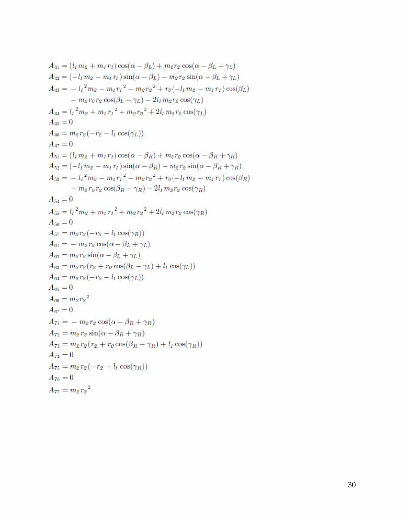
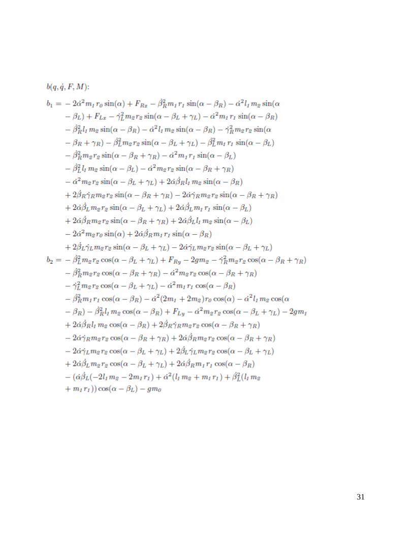
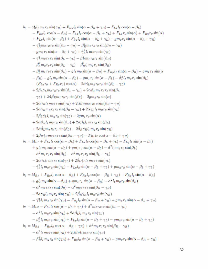
The vector q contains the generalized coordinates, F the ground support forces and M the joint moments.As the system has seven degrees of freedom, there exist also seven partial differential equations. The exact formulas of the inertia matrix A(q) and the right hand side are calculated as in Appendix A

2.2 Ground contact forces

2.2.1 Terminology A biped is an open kinematic chain consisting of two sub-chains called legs and, often, a sub-chain called the torso, all connected at a common point called the hip. One or both of the legs may be in contact with the ground. When only one leg is in contact with the ground, the contacting leg is called the stanceleg [1]and the other is called the swing leg. The end of a leg, whether it has links constituting a foot or not, will sometimes be referred to as a foot.

The single support or swing phase is defined to be the phase of locomotion where only one foot is on the ground. Conversely, double support is the phase where both feet are on the ground.Walking is then defined as alternating phases of single and double support, with the requirement that the displacement of the horizontal component of the robot’s center of mass. (COM) is strictly monotonic. Running is defined as sequential phases [2] of single support, flight, and (single-legged) impact, with the additional provision that impacts occur on alternating legs.

The sagittal plane is the longitudinal plane that divides the body into right and left sections. The frontal plane is the plane parallel to the long axis of the body and perpendicular to the sagittal plane that separates the body into front and back portions. The transverse plane is perpendicular to both the sagittal and frontal planes.

A planar biped is a biped with motions taking place only in the sagittal plane, whereas a three-dimensional walker has motions taking place in both the sagittal and frontal planes. A statically stable gait is periodic locomotion in which the biped’s COM does not leave the support polygon, that is, the convex hull formed by all of the contact points with the ground.

2.2.2 Why point feet? An important source of complexity in a biped system is the degree of actuationof the system, or more precisely, the degree of underactuation of the system.It will be assumed in this part of the

9

book that the legs are terminated in points, and consequently, no actuation is possible at the end of the stanceleg[3][4]. It follows that the system is underactuated during single support, asopposed to fully actuated (a control at each joint and at the contact pointwith the ground). During the flight phase of a running gait, the system isunderactuated in any case.One could be concerned that“real robots have feet,” and thus, while theanalysis of point-feet models may be of interest mathematically, it is“misguidedfor practical robotics.“Ifone takes human walking as the defacto standard against which mechanicalbipedal walking is to be compared, then the flat-footed walking achieved bycurrent robots needs to be improved[5]. In particular, toe roll toward the endof the single support phase needs to be allowed as part of the gait design.A model of an anthropomorphic walking gait should at least consider afully actuated phase where the stance foot is flat on the ground, followedby an underactuated phase where the stance heel lifts from the ground andthe stance foot rotates about the toe, and a double support phase whereleg exchange takes place; optionally, heel strike and heel roll could also beincluded, which would yield a second under actuated phase in the gait[6]. Ineither case, a model of walking with a point contact is an integral part of anoverall model of walking that is more anthropomorphic in nature than thecurrent flat-footed walking paradigm. Because the model with point feet issimpler than a more complete anthropomorphic gait model, it facilitates thedevelopment of new feedback designs and dynamic stability analysis methodsthat are appropriate for moving beyond quasi-static walking.

References

[1] K. Yin, “SIMBICON : Simple Biped Locomotion Control,” 2007.

[2] T. Wrigley, “Getting Data From Gait Traces,” Clin. Res., no. December, pp. 1–27, 2006.

[3] E. R. Westervelt, J. W. Grizzle, C. Chevallereau, J. H. Choi, and B. Morris, Feedback Control of Dynamic Bipedal Robot Locomotion. 2007.

[4] C.-L. Shih, “The Dynamics and Control of a Biped Walking Robot With Seven Degrees of Freedom,” J. Dyn. Syst. Meas. Control, vol. 118, no. December 1996, p. 683, 1996.

[5] R. Paper and A. P. Coimbra, “Tuning a PD Controller Based on an SVR for the Control of a Biped Robot Subject to External Forces and Slope Variation,” 2014.

[6] P. G. Oriolo, “Autonomous and Mobile Robotics Biped Robots 1 : Introduction and Passive Walking motivations sensible choice.”

10

3. SOFTWARE AND DETAILS OF PROJECT

This chapter explains about the MATLAB software and Simulink blocks along with details of the project such as Simulink blocks for the Knee angle limiter, Ground Contact forces, Biped model, PD model etc. along with various constraints.

3.1 About the Software- MATLAB & Simulink MATLAB (matrix laboratory) is a multi-paradigm numerical computing environment and fourth-generation programming language. Developed by MathWorks, MATLAB allows matrix manipulations, plotting of functions and data, implementation of algorithms, creation of user interfaces, and interfacing with programs written in other languages, including C, C++, Java, Fortran and Python. MathWorks offers tools and technologies for Model-Based Design that enable you to design complex, multidomain, time-varying systems that include controls, signal processing, communications, image and video processing, and cyber-physical system applications. This simulation-based approach gives you a better understanding of design alternatives and trade-offs than traditional prototype-based design methodologies, enabling you to optimize your design to meet predefined performance criteria.

By using these high-productivity tools in the design of your application, errors can be caught easily, tests can be done more thoroughly with multiple scenarios, robustness and sensitivity analyses can be carried out, and existing issues can be troubleshot effectively. This leads to key cost savings, shorter development cycles, fewer hardware prototypes, and high quality.

Simulink, developed by MathWorks, is a data flow graphical programming language tool for modelling, simulating and analyzing multidomain dynamic systems. Its primary interface is a graphical block diagramming tool and a customizable set of block libraries. It offers tight integration with the rest of the MATLAB environment and can either drive MATLAB or be scripted from it. Simulink is widely used in control theory and digital signal processing for multidomain simulation and Model-Based Design. Simulink® is a block diagram environment for multidomain simulation and Model-Based Design. It supports simulation, automatic code generation, and continuous test and verification of embedded systems.

Simulink provides a graphical editor, customizable block libraries, and solvers for modelling and simulating dynamic systems. It is integrated with MATLAB®, enabling you to incorporate MATLAB algorithms into models and export simulation results to MATLAB for further analysis.

It can help in building the model hierarchical subsystems with predefined library blocks, simulating the dynamic behaviour of your system and view results as the simulation runs. Adding to this, it can analyze simulation results, debug the simulation, easily manage files, components, and large amounts of data for your project.

11

Model-Based Design is transforming the way engineers and scientists work by moving design tasks from the lab and field to the desktop.

When software and hardware implementation requirements are included, such as fixed-point and timing behaviour, you can automatically generate code for embedded deployment and create test benches for system verification, saving time and avoiding the introduction of manually coded errors.

Use Model-Based Design with MATLAB® and Simulink® to improve product quality and reduce development time by 50% or more.

3.2 Details of the project We used Matlab Software and Simulink to construct our Biped model.

The code model is divided into 4 parts:

1. PD control 2. Add noise 3. Biped model 4. Detect falling

3.3 PD control

3.3.1 PDref controller

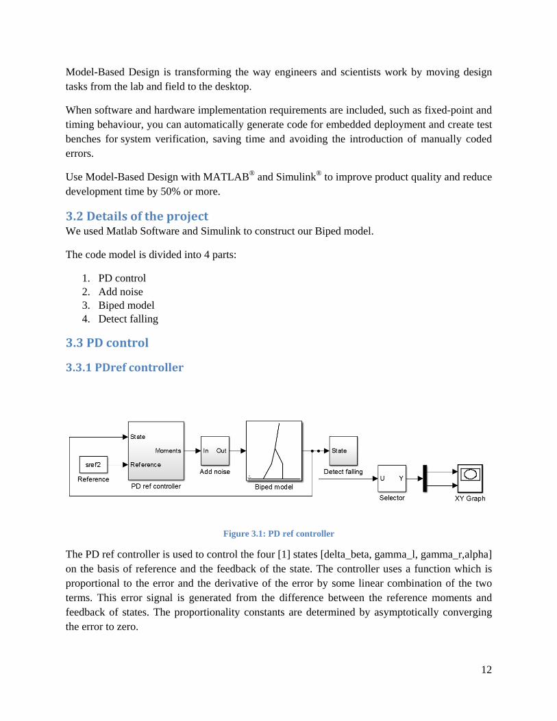
Figure 3.1: PD ref controller

The PD ref controller is used to control the four [1] states [delta_beta, gamma_l, gamma_r,alpha] on the basis of reference and the feedback of the state. The controller uses a function which is proportional to the error and the derivative of the error by some linear combination of the two terms. This error signal is generated from the difference between the reference moments and feedback of states. The proportionality constants are determined by asymptotically converging the error to zero.

12

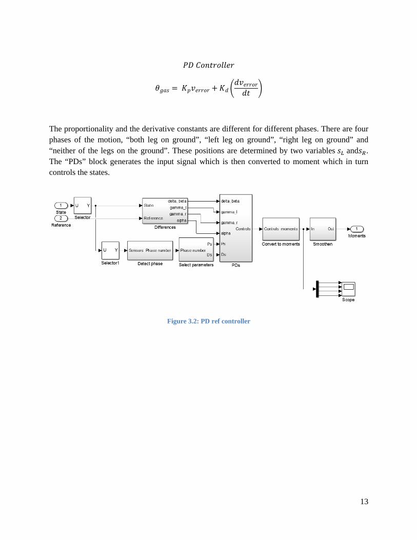
𝑃𝑃𝑃𝑃 𝐶𝐶𝐶𝐶𝐶𝐶𝐶𝐶𝐶𝐶𝐶𝐶𝐶𝐶𝐶𝐶𝐶𝐶𝐶𝐶

𝜃𝜃𝑔𝑔𝑔𝑔𝑔𝑔 = 𝐾𝐾𝑝𝑝𝑣𝑣𝐶𝐶𝐶𝐶𝐶𝐶𝐶𝐶𝐶𝐶 +𝐾𝐾𝑑𝑑 �𝑑𝑑𝑣𝑣𝐶𝐶𝐶𝐶𝐶𝐶𝐶𝐶𝐶𝐶𝑑𝑑𝐶𝐶 �

The proportionality and the derivative constants are different for different phases. There are four phases of the motion, “both leg on ground”, “left leg on ground”, “right leg on ground” and “neither of the legs on the ground”. These positions are determined by two variables 𝑔𝑔𝐿𝐿 and𝑔𝑔𝑅𝑅. The “PDs” block generates the input signal which is then converted to moment which in turn controls the states.

Figure 3.2: PD ref controller

13

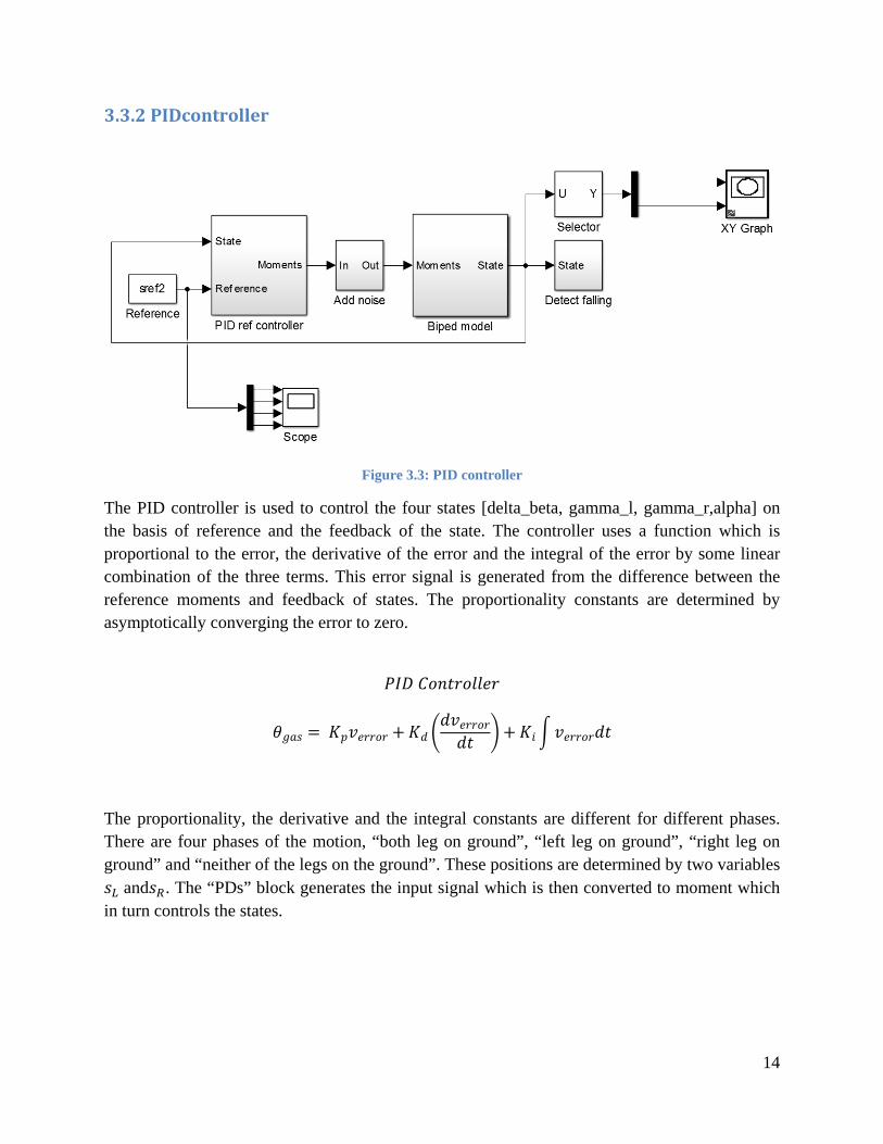
3.3.2 PIDcontroller

Figure 3.3: PID controller

The PID controller is used to control the four states [delta_beta, gamma_l, gamma_r,alpha] on the basis of reference and the feedback of the state. The controller uses a function which is proportional to the error, the derivative of the error and the integral of the error by some linear combination of the three terms. This error signal is generated from the difference between the reference moments and feedback of states. The proportionality constants are determined by asymptotically converging the error to zero.

𝑃𝑃𝑃𝑃𝑃𝑃 𝐶𝐶𝐶𝐶𝐶𝐶𝐶𝐶𝐶𝐶𝐶𝐶𝐶𝐶𝐶𝐶𝐶𝐶𝐶𝐶

𝜃𝜃𝑔𝑔𝑔𝑔𝑔𝑔 = 𝐾𝐾𝑝𝑝𝑣𝑣𝐶𝐶𝐶𝐶𝐶𝐶𝐶𝐶𝐶𝐶 +𝐾𝐾𝑑𝑑 �𝑑𝑑𝑣𝑣𝐶𝐶𝐶𝐶𝐶𝐶𝐶𝐶𝐶𝐶𝑑𝑑𝐶𝐶 � +𝐾𝐾𝑖𝑖 �𝑣𝑣𝐶𝐶𝐶𝐶𝐶𝐶𝐶𝐶𝐶𝐶𝑑𝑑𝐶𝐶

The proportionality, the derivative and the integral constants are different for different phases. There are four phases of the motion, “both leg on ground”, “left leg on ground”, “right leg on ground” and “neither of the legs on the ground”. These positions are determined by two variables 𝑔𝑔𝐿𝐿 and𝑔𝑔𝑅𝑅. The “PDs” block generates the input signal which is then converted to moment which in turn controls the states.

14

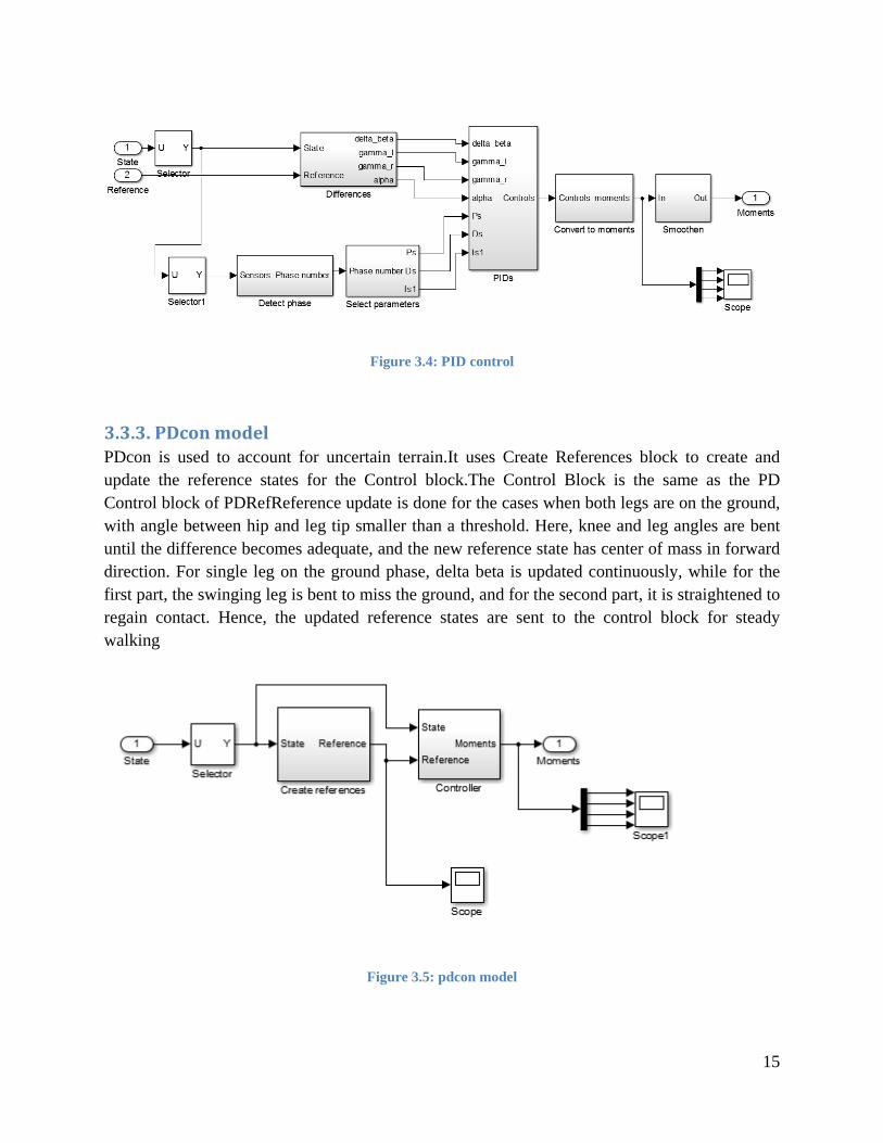
Figure 3.4: PID control

3.3.3. PDcon model PDcon is used to account for uncertain terrain.It uses Create References block to create and update the reference states for the Control block.The Control Block is the same as the PD Control block of PDRefReference update is done for the cases when both legs are on the ground, with angle between hip and leg tip smaller than a threshold. Here, knee and leg angles are bent until the difference becomes adequate, and the new reference state has center of mass in forward direction. For single leg on the ground phase, delta beta is updated continuously, while for the first part, the swinging leg is bent to miss the ground, and for the second part, it is straightened to regain contact. Hence, the updated reference states are sent to the control block for steady walking

Figure 3.5: pdcon model

15

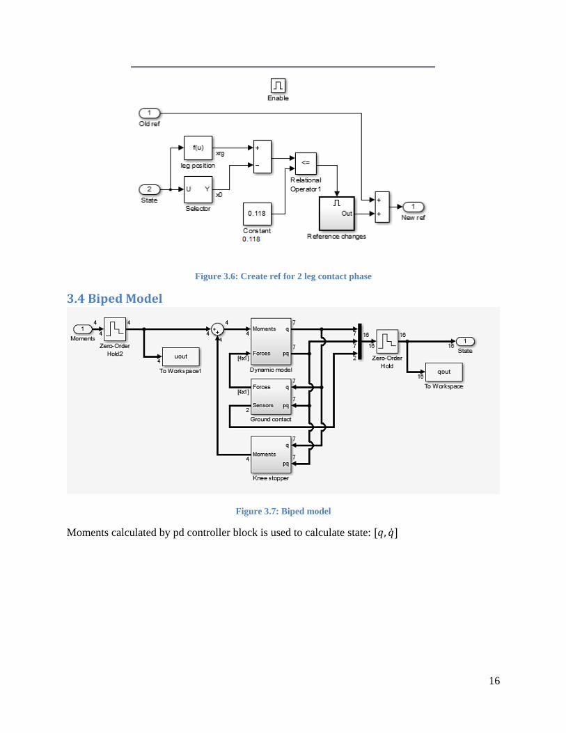
Figure 3.6: Create ref for 2 leg contact phase

3.4 Biped Model

Figure 3.7: Biped model

Moments calculated by pd controller block is used to calculate state: [𝑞𝑞, �̇�𝑞]

16

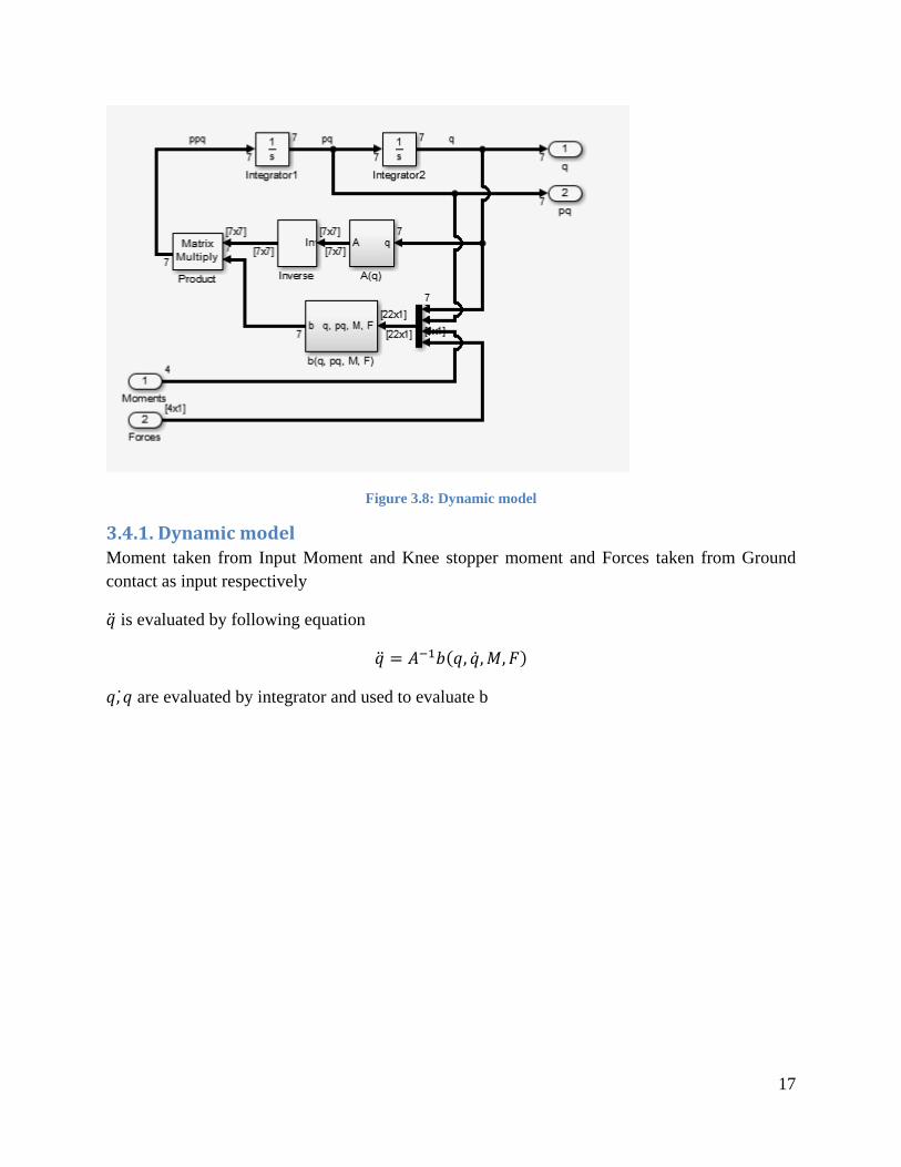
Figure 3.8: Dynamic model

3.4.1. Dynamic model Moment taken from Input Moment and Knee stopper moment and Forces taken from Ground contact as input respectively

�̈�𝑞 is evaluated by following equation

�̈�𝑞 = 𝐴𝐴−1𝑏𝑏(𝑞𝑞, �̇�𝑞,𝑀𝑀,𝐹𝐹)

𝑞𝑞, 𝑞𝑞̇ are evaluated by integrator and used to evaluate b

17

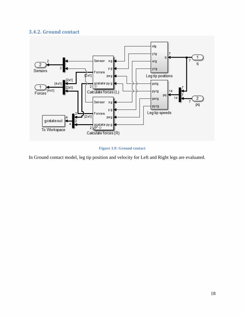
3.4.2. Ground contact

Figure 3.9: Ground contact

In Ground contact model, leg tip position and velocity for Left and Right legs are evaluated.

18

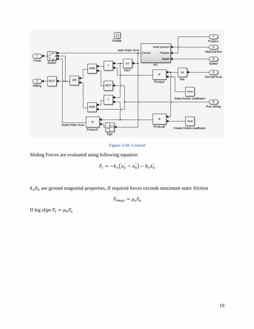
Figure 3.10: Control

Sliding Forces are evaluated using following equation

𝐹𝐹𝑡𝑡 = −𝑘𝑘𝑥𝑥�𝑥𝑥𝐺𝐺′ − 𝑥𝑥0′ � − 𝑏𝑏𝑥𝑥�̇�𝑥𝐺𝐺′

𝑘𝑘𝑥𝑥𝑏𝑏𝑥𝑥 are ground tangential properties, If required forces exceeds maximum static friction

𝐹𝐹𝑡𝑡𝑡𝑡𝑡𝑡𝑥𝑥 = 𝜇𝜇𝑠𝑠𝐹𝐹𝑛𝑛

If leg slips 𝐹𝐹𝑡𝑡 = 𝜇𝜇𝑘𝑘𝐹𝐹𝑛𝑛

19

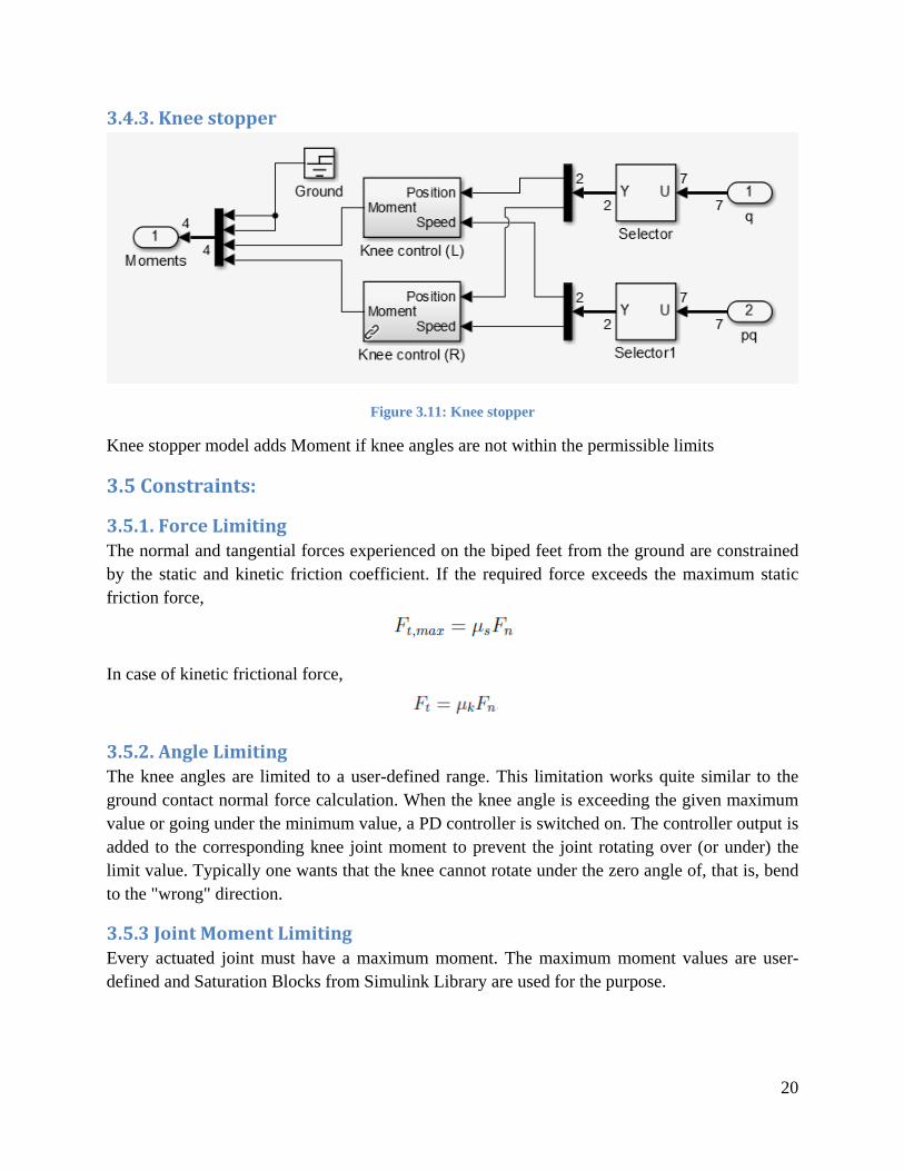
3.4.3. Knee stopper

Figure 3.11: Knee stopper

Knee stopper model adds Moment if knee angles are not within the permissible limits

3.5 Constraints:

3.5.1. Force Limiting The normal and tangential forces experienced on the biped feet from the ground are constrained by the static and kinetic friction coefficient. If the required force exceeds the maximum static friction force,

In case of kinetic frictional force,

3.5.2. Angle Limiting The knee angles are limited to a user-defined range. This limitation works quite similar to the ground contact normal force calculation. When the knee angle is exceeding the given maximum value or going under the minimum value, a PD controller is switched on. The controller output is added to the corresponding knee joint moment to prevent the joint rotating over (or under) the limit value. Typically one wants that the knee cannot rotate under the zero angle of, that is, bend to the "wrong" direction.

3.5.3 Joint Moment Limiting Every actuated joint must have a maximum moment. The maximum moment values are user-defined and Saturation Blocks from Simulink Library are used for the purpose.

20

3.6. Dimensioning The dimensions of the Biped model are stored in the MATLAB file bipedparams.m (Appendix B)

References [1] O. Haavisto and H. Hyötyniemi, “Simulation tool of a biped walking robot model,” Helsinki, Finland, 2004.

21

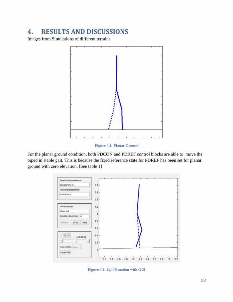
4. RESULTS AND DISCUSSIONS Images from Simulations of different terrains

Figure 4.1: Planar Ground

For the planar ground condition, both PDCON and PDREF control blocks are able to move the biped in stable gait. This is because the fixed reference state for PDREF has been set for planar ground with zero elevation. [See table 1]

Figure 4.2: Uphill motion with GUI

22

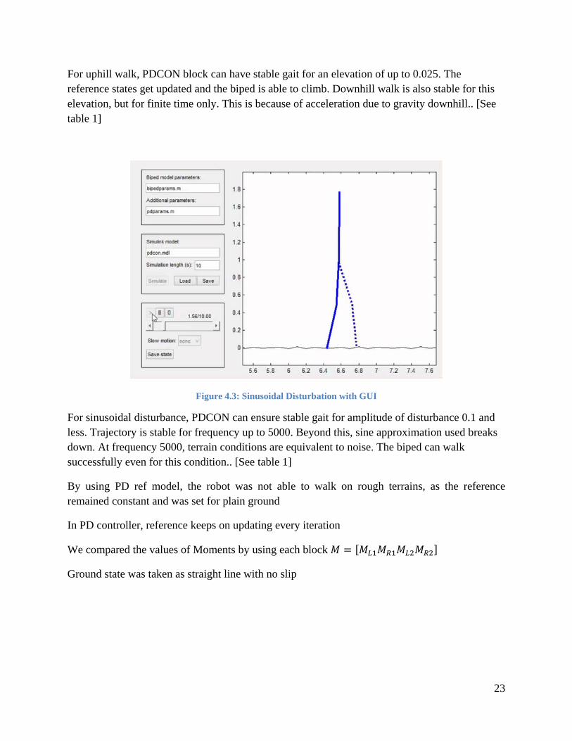
For uphill walk, PDCON block can have stable gait for an elevation of up to 0.025. The reference states get updated and the biped is able to climb. Downhill walk is also stable for this elevation, but for finite time only. This is because of acceleration due to gravity downhill.. [See table 1]

Figure 4.3: Sinusoidal Disturbation with GUI

For sinusoidal disturbance, PDCON can ensure stable gait for amplitude of disturbance 0.1 and less. Trajectory is stable for frequency up to 5000. Beyond this, sine approximation used breaks down. At frequency 5000, terrain conditions are equivalent to noise. The biped can walk successfully even for this condition.. [See table 1]

By using PD ref model, the robot was not able to walk on rough terrains, as the reference remained constant and was set for plain ground

In PD controller, reference keeps on updating every iteration

We compared the values of Moments by using each block 𝑀𝑀 = [𝑀𝑀𝐿𝐿1𝑀𝑀𝑅𝑅1𝑀𝑀𝐿𝐿2𝑀𝑀𝑅𝑅2]

Ground state was taken as straight line with no slip

23

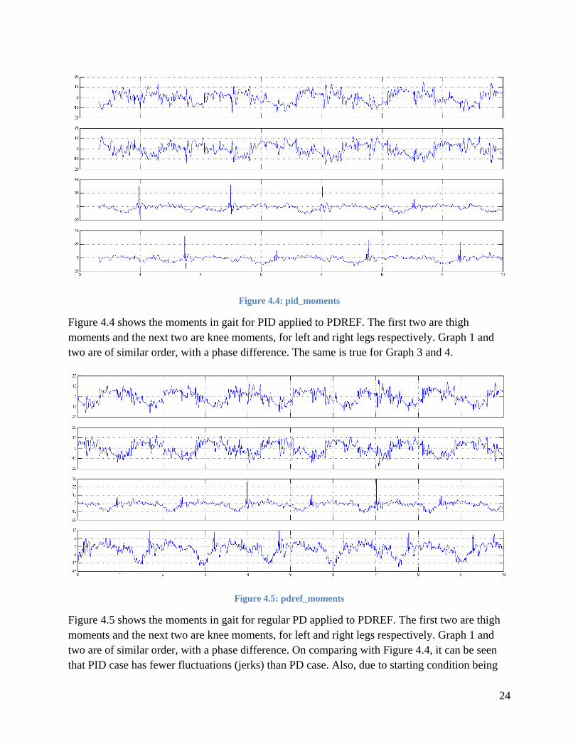
Figure 4.4: pid_moments

Figure 4.4 shows the moments in gait for PID applied to PDREF. The first two are thigh moments and the next two are knee moments, for left and right legs respectively. Graph 1 and two are of similar order, with a phase difference. The same is true for Graph 3 and 4.

Figure 4.5: pdref_moments

Figure 4.5 shows the moments in gait for regular PD applied to PDREF. The first two are thigh moments and the next two are knee moments, for left and right legs respectively. Graph 1 and two are of similar order, with a phase difference. On comparing with Figure 4.4, it can be seen that PID case has fewer fluctuations (jerks) than PD case. Also, due to starting condition being

24

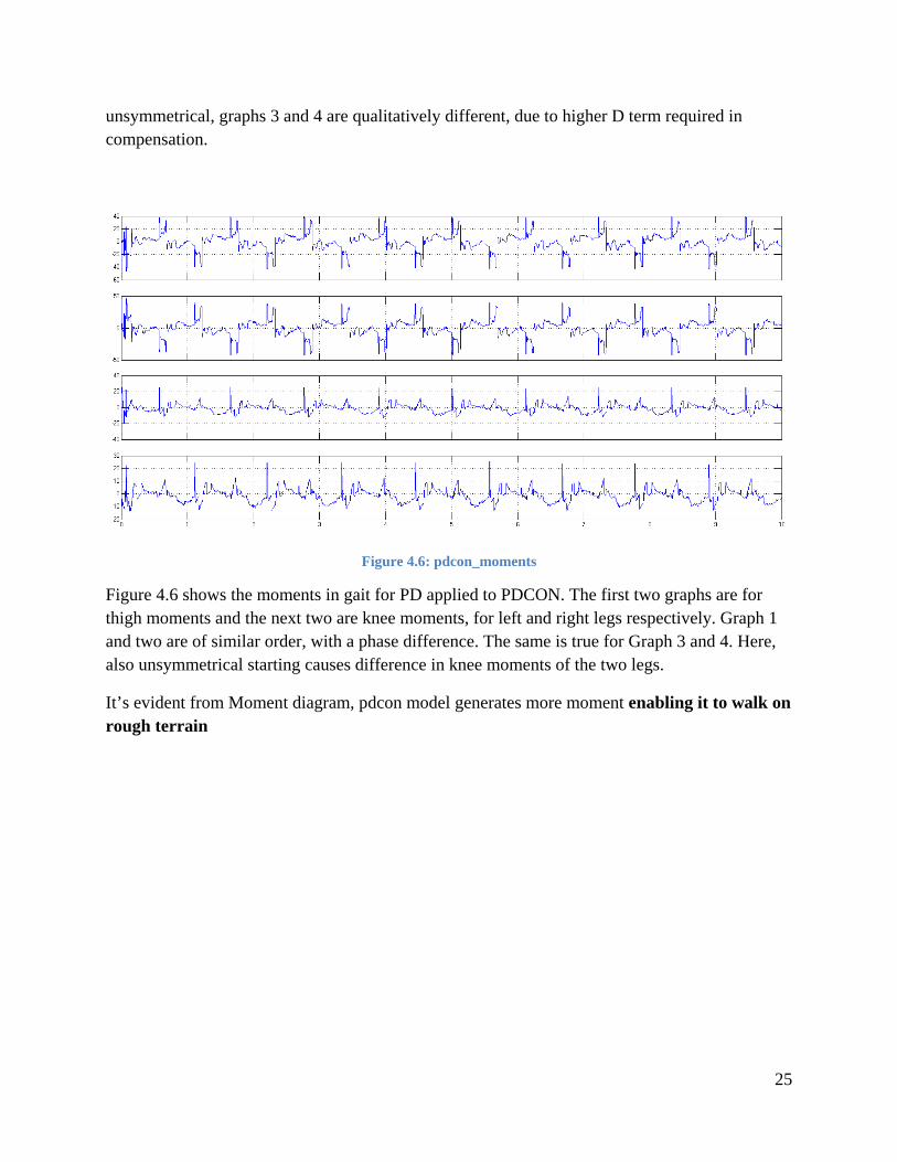
unsymmetrical, graphs 3 and 4 are qualitatively different, due to higher D term required in compensation.

Figure 4.6: pdcon_moments

Figure 4.6 shows the moments in gait for PD applied to PDCON. The first two graphs are for thigh moments and the next two are knee moments, for left and right legs respectively. Graph 1 and two are of similar order, with a phase difference. The same is true for Graph 3 and 4. Here, also unsymmetrical starting causes difference in knee moments of the two legs.

It’s evident from Moment diagram, pdcon model generates more moment enabling it to walk on rough terrain

25

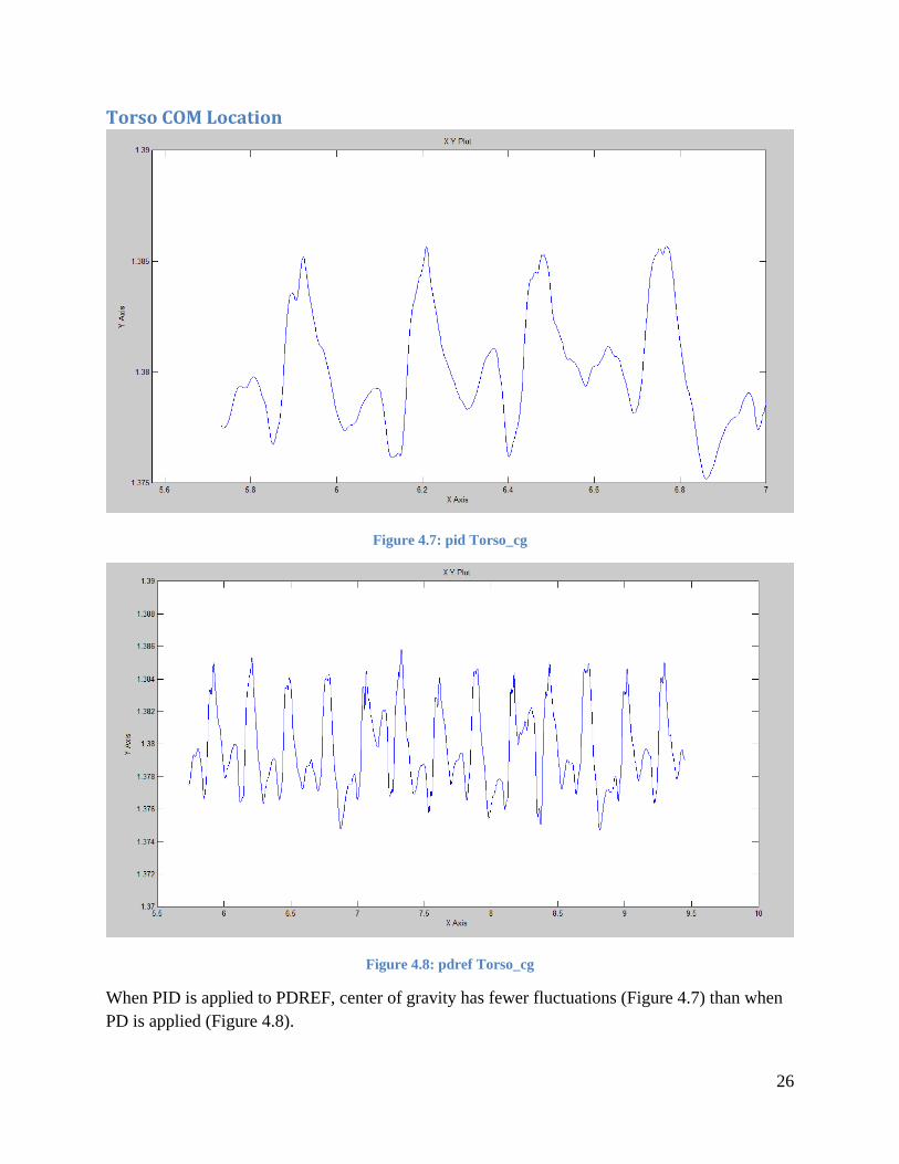
Torso COM Location

Figure 4.7: pid Torso_cg

Figure 4.8: pdref Torso_cg

When PID is applied to PDREF, center of gravity has fewer fluctuations (Figure 4.7) than when PD is applied (Figure 4.8).

26

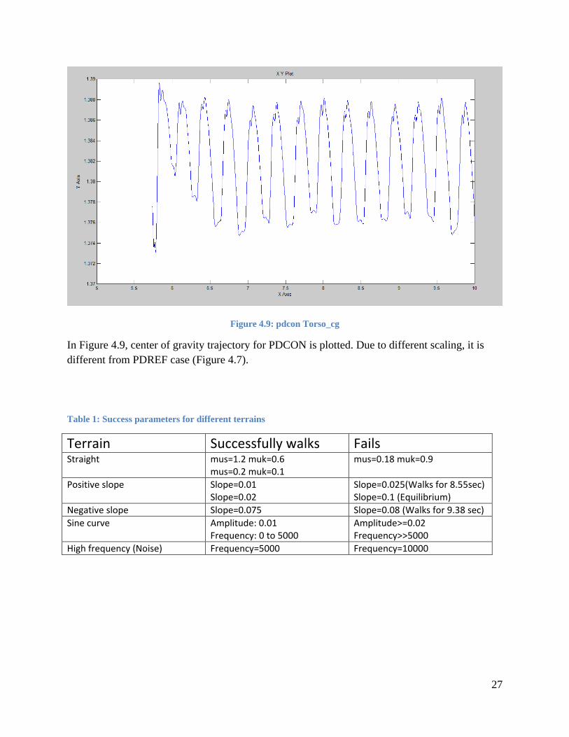
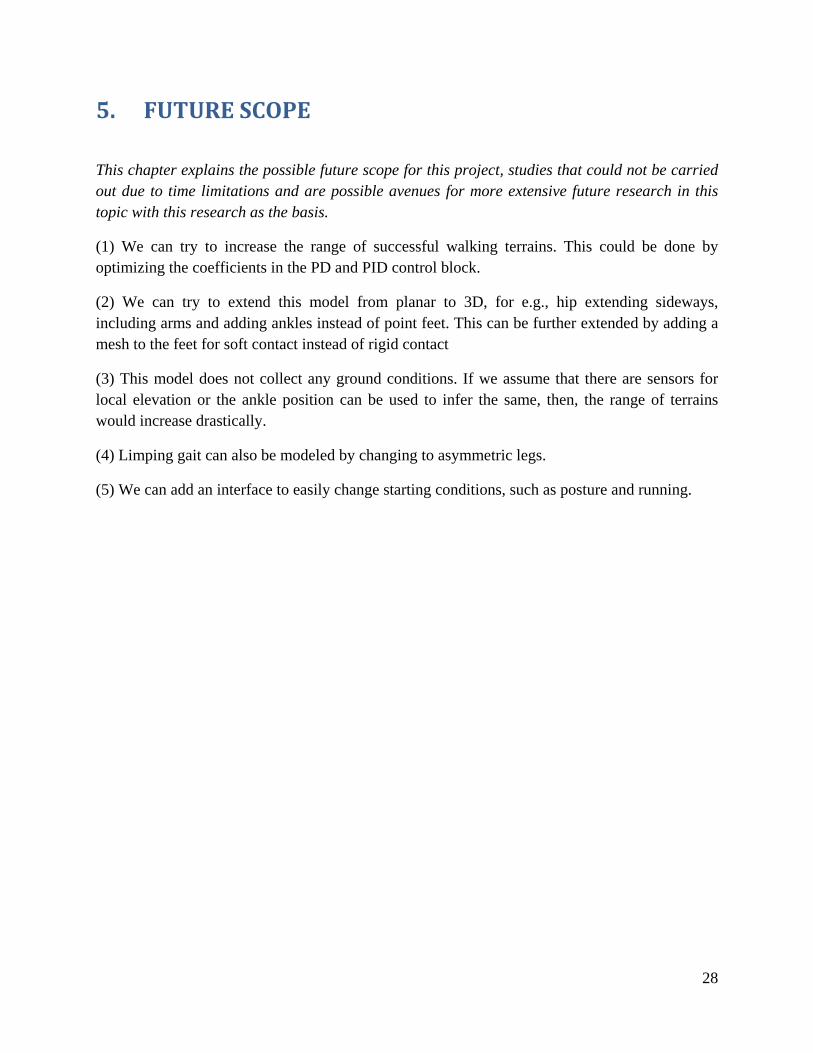
Figure 4.9: pdcon Torso_cg

In Figure 4.9, center of gravity trajectory for PDCON is plotted. Due to different scaling, it is different from PDREF case (Figure 4.7).

Table 1: Success parameters for different terrains

Terrain Successfully walks Fails Straight mus=1.2 muk=0.6

mus=0.2 muk=0.1 mus=0.18 muk=0.9

Positive slope Slope=0.01 Slope=0.02

Slope=0.025(Walks for 8.55sec) Slope=0.1 (Equilibrium)

Negative slope Slope=0.075 Slope=0.08 (Walks for 9.38 sec) Sine curve Amplitude: 0.01

Frequency: 0 to 5000 Amplitude>=0.02 Frequency>>5000

High frequency (Noise) Frequency=5000 Frequency=10000

27

5. FUTURE SCOPE

This chapter explains the possible future scope for this project, studies that could not be carried out due to time limitations and are possible avenues for more extensive future research in this topic with this research as the basis.

(1) We can try to increase the range of successful walking terrains. This could be done by optimizing the coefficients in the PD and PID control block.

(2) We can try to extend this model from planar to 3D, for e.g., hip extending sideways, including arms and adding ankles instead of point feet. This can be further extended by adding a mesh to the feet for soft contact instead of rigid contact

(3) This model does not collect any ground conditions. If we assume that there are sensors for local elevation or the ankle position can be used to infer the same, then, the range of terrains would increase drastically.

(4) Limping gait can also be modeled by changing to asymmetric legs.

(5) We can add an interface to easily change starting conditions, such as posture and running.

28

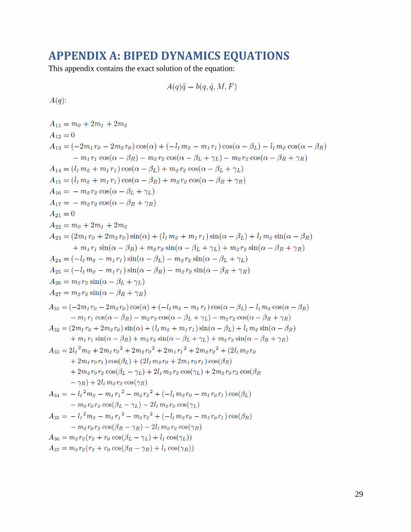
APPENDIX A: BIPED DYNAMICS EQUATIONS This appendix contains the exact solution of the equation:

29

30

31

32

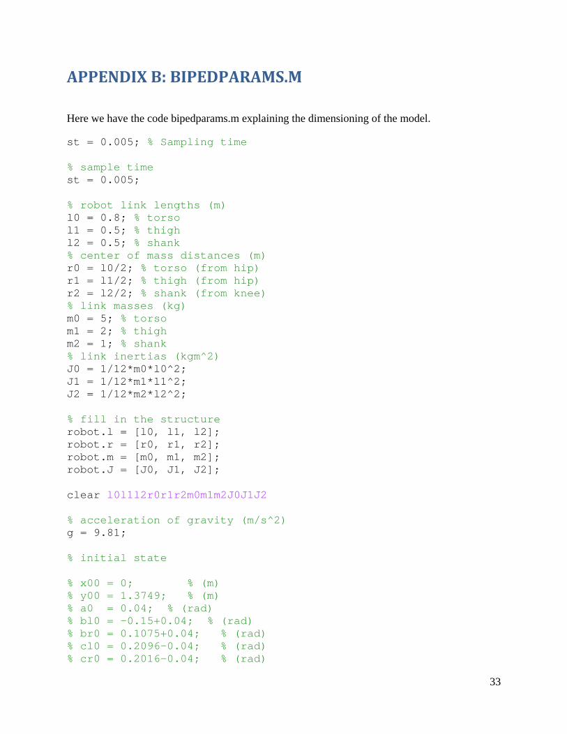
APPENDIX B: BIPEDPARAMS.M

Here we have the code bipedparams.m explaining the dimensioning of the model.

st = 0.005; % Sampling time % sample time st = 0.005; % robot link lengths (m) l0 = 0.8; % torso l1 = 0.5; % thigh l2 = 0.5; % shank % center of mass distances (m) r0 = l0/2; % torso (from hip) r1 = l1/2; % thigh (from hip) r2 = l2/2; % shank (from knee) % link masses (kg) m0 = 5; % torso m1 = 2; % thigh m2 = 1; % shank % link inertias (kgm^2) J0 = 1/12*m0*l0^2; J1 = 1/12*m1*l1^2; J2 = 1/12*m2*l2^2; % fill in the structure robot.l = [l0, l1, l2]; robot.r = [r0, r1, r2]; robot.m = [m0, m1, m2]; robot.J = [J0, J1, J2]; clear l0l1l2r0r1r2m0m1m2J0J1J2 % acceleration of gravity (m/s^2) g = 9.81; % initial state % x00 = 0; % (m) % y00 = 1.3749; % (m) % a0 = 0.04; % (rad) % bl0 = -0.15+0.04; % (rad) % br0 = 0.1075+0.04; % (rad) % cl0 = 0.2096-0.04; % (rad) % cr0 = 0.2016-0.04; % (rad)

33

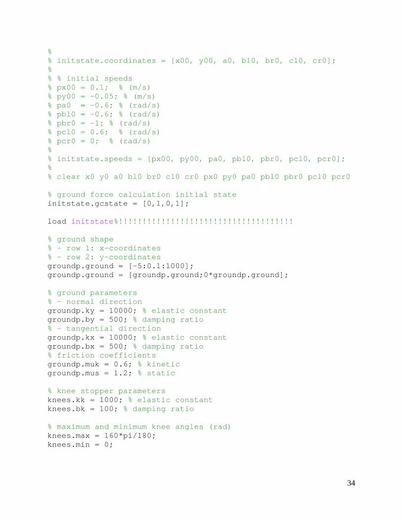
% % initstate.coordinates = [x00, y00, a0, bl0, br0, cl0, cr0]; % % % initial speeds % px00 = 0.1; % (m/s) % py00 = -0.05; % (m/s) % pa0 = -0.6; % (rad/s) % pbl0 = -0.6; % (rad/s) % pbr0 = -1; % (rad/s) % pcl0 = 0.6; % (rad/s) % pcr0 = 0; % (rad/s) % % initstate.speeds = [px00, py00, pa0, pbl0, pbr0, pcl0, pcr0]; % % clear x0 y0 a0 bl0 br0 cl0 cr0 px0 py0 pa0 pbl0 pbr0 pcl0 pcr0 % ground force calculation initial state initstate.gcstate = [0,1,0,1]; load initstate%!!!!!!!!!!!!!!!!!!!!!!!!!!!!!!!!!!!!! % ground shape % - row 1: x-coordinates % - row 2: y-coordinates groundp.ground = [-5:0.1:1000]; groundp.ground = [groundp.ground;0*groundp.ground]; % ground parameters % - normal direction groundp.ky = 10000; % elastic constant groundp.by = 500; % damping ratio % - tangential direction groundp.kx = 10000; % elastic constant groundp.bx = 500; % damping ratio % friction coefficients groundp.muk = 0.6; % kinetic groundp.mus = 1.2; % static % knee stopper parameters knees.kk = 1000; % elastic constant knees.bk = 100; % damping ratio % maximum and minimum knee angles (rad) knees.max = 160*pi/180; knees.min = 0;

34

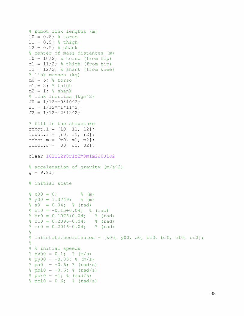
% robot link lengths (m) l0 = 0.8; % torso l1 = 0.5; % thigh l2 = 0.5; % shank % center of mass distances (m) r0 = l0/2; % torso (from hip) r1 = l1/2; % thigh (from hip) r2 = l2/2; % shank (from knee) % link masses (kg) m0 = 5; % torso m1 = 2; % thigh m2 = 1; % shank % link inertias (kgm^2) J0 = 1/12*m0*l0^2; J1 = 1/12*m1*l1^2; J2 = 1/12*m2*l2^2; % fill in the structure robot.l = [l0, l1, l2]; robot.r = [r0, r1, r2]; robot.m = [m0, m1, m2]; robot.J = [J0, J1, J2]; clear l0l1l2r0r1r2m0m1m2J0J1J2 % acceleration of gravity (m/s^2) g = 9.81; % initial state % x00 = 0; % (m) % y00 = 1.3749; % (m) % a0 = 0.04; % (rad) % bl0 = -0.15+0.04; % (rad) % br0 = 0.1075+0.04; % (rad) % cl0 = 0.2096-0.04; % (rad) % cr0 = 0.2016-0.04; % (rad) % % initstate.coordinates = [x00, y00, a0, bl0, br0, cl0, cr0]; % % % initial speeds % px00 = 0.1; % (m/s) % py00 = -0.05; % (m/s) % pa0 = -0.6; % (rad/s) % pbl0 = -0.6; % (rad/s) % pbr0 = -1; % (rad/s) % pcl0 = 0.6; % (rad/s)

35

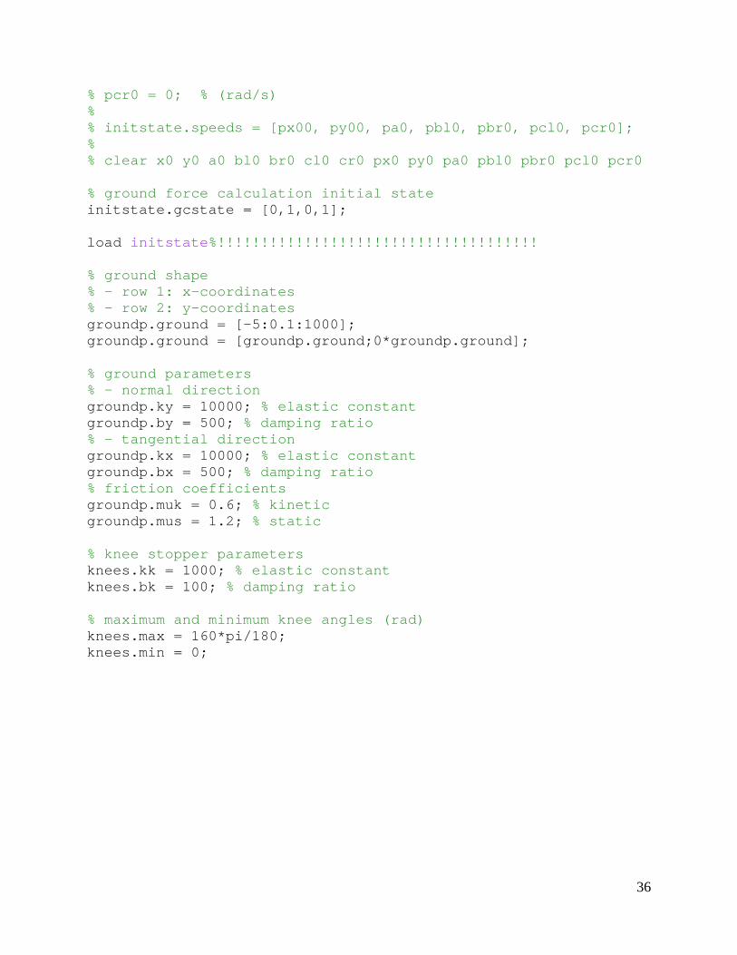
% pcr0 = 0; % (rad/s) % % initstate.speeds = [px00, py00, pa0, pbl0, pbr0, pcl0, pcr0]; % % clear x0 y0 a0 bl0 br0 cl0 cr0 px0 py0 pa0 pbl0 pbr0 pcl0 pcr0 % ground force calculation initial state initstate.gcstate = [0,1,0,1]; load initstate%!!!!!!!!!!!!!!!!!!!!!!!!!!!!!!!!!!!!! % ground shape % - row 1: x-coordinates % - row 2: y-coordinates groundp.ground = [-5:0.1:1000]; groundp.ground = [groundp.ground;0*groundp.ground]; % ground parameters % - normal direction groundp.ky = 10000; % elastic constant groundp.by = 500; % damping ratio % - tangential direction groundp.kx = 10000; % elastic constant groundp.bx = 500; % damping ratio % friction coefficients groundp.muk = 0.6; % kinetic groundp.mus = 1.2; % static % knee stopper parameters knees.kk = 1000; % elastic constant knees.bk = 100; % damping ratio % maximum and minimum knee angles (rad) knees.max = 160*pi/180; knees.min = 0;

36