Using math to defeat the enemy (7 7-2011)

Approved for Public Release

Simulation Educators, LLC (29 June 2011)

Jeffrey Strickland, Ph.D., CMSP

1DISTRIBUTION STATEMENT A. Approved for

public release; distribution is unlimited.

http://www.modelingandsimulationevent.com/Event.aspx?id=512230


http://www.idga.org/

http://www.idga.org/



Learning Objectives

1. Describe the scope of mathematical and heuristic

combat models.

2. Compare and contrast different representations of

combat phenomenon.

3. List combat behaviors that can be represented by

mathematical & heuristic models.

4. State the various types of mathematical and

heuristic combat models.

5. Identify examples of mathematical and heuristic

combat models.

2Copyright© 2010 Jeffrey Strickland, Ph.D.





Tutorial Outline

Environmental modeling how to model the

environment

level of detail

entity interaction

Physical modeling how to move

how to sense or detect

how to shoot (or create other effects)

how to communicate

Simulation scenario development what are the elements of a

scenario

how to develop scenarios

Missile Flight Modeling Missile dynamics

Sensor dynamics

Racking error

Coordinate systems

Simulation

Results

Simulation scenario development what are the elements of a

scenario

how to develop scenarios






Level of Detail

Conceptual Reference Model

Data Collection

Data Processing

Static Environment

Dynamic Environment

Standardization






Level of Detail

Perceived details bitmaps over data points

hills, trees, rivers, rocks

No interaction simulated system does not

interact directly with terrain details.

Visual detail polygon color & lighting bit mapped surfaces hard surfaces

Modeling detail surface trafficability foliage density tree trunk diameter

5

Air Combat Terrain Ground Combat Terrain

Copyright© 2010 Jeffrey Strickland, Ph.D.





Conceptual Reference Model

6

Component

Models

Environmental

State

Behavior

Models

Environmental

Models

Synthetic Natural Environment

Behaviors (e.g.)

• Maneuver

• Sustainment

• Force

Protection

• Intelligence

• Command &

Control

• Fires

Military System Model

Effects (e.g.)

• Attenuation

• Propagation

• Mobility

Internal Dynamics

Impacts (e.g.)

• Obscurants/

Energy (smoke,

chaff, spectral,..)

• Damage

(engrg, craters,..)

Data (e.g.)

• Terrain

(surface, hydro,..)

• Atmosphere

(aerosols, clouds,..)

• Ocean

(sea state, SVP,..)

• Space

(particle flux,..)

• Cultural

(roads, structures,..)

• Military

(engrg. works,..)

Passive

Sensors

Active

Sensors

Weapons &

Countermeasures

Units/Platforms

SOURCE: Paul A. Birkel, "SNE Conceptual Reference Model", 1999 Fall SIW Conference, September 1999.

http://www.sisostds.org/siw/98Fall/view-papers.htm






Data Processing

7

Collection

• survey the environment (satellite, maps, etc.)

• store the results

• vector, grid, and model data

Cleaning

• remove collection process discontinuities

• synchronize vector and grid data

Organizing

• index and archive

Integration

• merge vector, grid, model

• generate terrain skin with embedded features and surface data

Transmission

• move data to the host system

Compilation

• create performance-optimized runtime databases

• cut into sheets




http://spatialnews.geocomm.com/images/sts99crew_large.jpg

http://spatialnews.geocomm.com/images/sts99crew_large.jpg



Landclass Terrain in AVSIM FSX The scenery engine in FSX, as with previous versions, uses the Olson Global Ecosystem

Legend, a table of terrain coverage types created by the USGS Earth Resources

Observation and Science Center (EROS). This data, called landclass data, is used by the

simulator to associate up to 255 types of terrain to map the entire surface of the globe. The

smallest level of detail is 1.2 square kilometers (0.46 square miles).

The landclass data is used by the simulator to select textures and objects to render the

scenery. The table below shows an example of the Olson classes used in FSX:

8

0 Ocean, Sea, Large Lake 40 Cool Grasses And Shrubs 131 Dirt

1 Large City Urban Grid Wet 41 Hot And Mild Grasses And Shrubs 132 Coral

2 Low Sparse Grassland 42 Cold Grassland 133 Lava

3 Coniferous Forest 43 Savanna (Woods) 134 Park

4 Deciduous Conifer Forest 44 Mire Bog Fen 135 Golf Course

5 Deciduous Broadleaf Forest 45 Marsh Wetland 136 Cement

20 Cool Rain Forest 46 Mediterranean Scrub 137 Tan Sand Beach

27 Conifer Forest 53 Barren Tundra 143 Glacier Ice

29 Seasonal Tropical Forest 54 Cool Southern Hemisphere Mixed Forests 144 Evergreen Tree Crop

33 Tropical Rainforest 60 Small Leaf Mixed Woods 146 Desert Rock




http://www.avsim.com/pages/0308/SceneryTech/geneva 2 fsx.jpg

http://www.avsim.com/pages/0308/SceneryTech/geneva 2 fsx.jpg

http://www.avsim.com/pages/0308/SceneryTech/murmansk 3 fsx.jpg

http://www.avsim.com/pages/0308/SceneryTech/murmansk 3 fsx.jpg



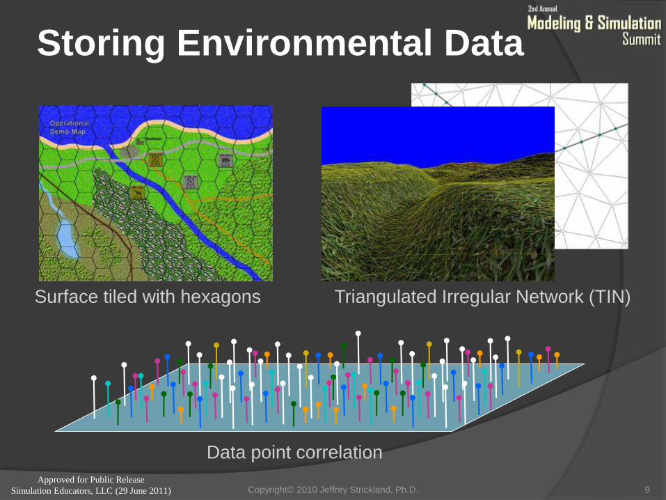
Storing Environmental Data

9

Triangulated Irregular Network (TIN)

Data point correlation

Surface tiled with hexagons






Static Environment

10

Trafficability

Terrain Type

Visibility






Landclass Terrain in EADSIM

Name: Desert (radiobutton) Description: If selected, the LANDCL model will assume desert

terrain.

Restrictions: Ghosted unless LANDCL Reflectivity is selected.

Name: Farmland (radiobutton) Description: If selected, the LANDCL model will assume farmland

terrain.


Name: Wooded Hills (radiobutton) Description: If selected, the LANDCL model will assume wooded hill

terrain.


Name: Mountains (radiobutton) Description: If selected, the LANDCL model will assume

mountainous terrain.







Dynamic Environment

12

Independent

• weather movement –clouds, rain, wind

• sea state – storms, daily tide

• daylight – sunrise, sunset, dark

• smoke & dust – clouds, raising, dispersing

Interaction

• holes – artillery craters, engineering artifacts

• tank treads – tracks, destruction

• terrain morphing –engineering, construction

• feature modification –building damage, trees burned






Classic Problems in Interpretation

13

1

2

3a 3b

1

2a 2b

Terrain Points Building Corners






Environmental Standardization






Physical Modeling

15

Detect/Acquire

Engage(other major

combat functions)

Communicate

Move

Start Cycle Here






Movement Points Movement

Bald Earth Movement

Terrain and Feature Movement

Physics-based Movement

Automated Route Planning

A* Search

Topology Smart

Grid Registration

Behavioral






Movement Points Movement

17

2

3

6

1

2 6 2

1

Movement

Points =

20

Movement

Points

Remaining =

20 – 11 = 9






Bald Earth Movement

18

Set heading, speed, start time

Rate*Time = Distance

20 km/hr * 30 min = 10 km






Terrain and Feature Movement

19

Set Objective: position or vector

Terrain & features modify instantaneous heading & speed

Speed = min(order_speed, max_speed*trafficability*slope_factor)*

weather_factor*lighting_factor*fatigue_factor*supression_factor






Physics-based Movement

20

Proportional Force

Calculation

Resistive Force

Calculation

Braking Force

Calculation

main force calculations

Dynamic

Equation

Calculations

net force

new vehicle state

(pos, vel, acc)

Vehicle type, terrain

type, slope, controls,

current platform state

The CCTT ground vehicle mobility

model is based on a general first-

principle dynamics model.

The model integrates explicit

driver inputs (e.g., throttle, brake)

with vehicle class-specific velocity,

resistance force, and deceleration

pre-computed curves.

Simple View of a Dynamic

Movement Model

CCTT Vehicle Dynamics Block Diagram






Automatic Route Planning

CONCEPT: provide an algorithm by which units can automatically find their own routes. allows the analyst to focus on higher issues such as the

overall scheme of maneuver reduces the intrusion of the analyst into C2 units can still be given explicit routes if desired, or closely

grouped intermediate objectives

ALGORITHMS: based on graph theory could be a satisfying algorithm (not guaranteed to find an

optimal route) might be an optimal algorithm “optimal" may mean fastest, or shortest, or safest, etc.

EXAMPLES A* search, Johnson’s algorithm, Dijkstra's algorithm, hill

climbing






Topology Smart

22

Set Objective: Position or Vector

Movement model selects path from topological map

Maintain objective

Route traveled is function of topology






Beyond 2-D Movement

3 Dimensional—aircraft rotation axes

yaw - vertical axis rotation

roll - longitudinal axis rotation

pitch- lateral axis rotation

3-D Mathematics

Euler angles

axis angle

rotation matrices

quaternions

Other degrees of freedom: 3+3 DOF, 6

DOF

23

Pitch

Yaw

Roll






Behavioral—Agent Based

Behavioral evolution and extrapolation

Each avatar generates (a) a stream of ghosts samples the personality space of its entity.

They evolve (b, c) against the entity’s recent observed behavior.

The fittest ghosts run into the future (d),

and the avatar analyzes their behavior (e) to generate predictions.

24

a

b

e

d

Prediction Horizon

Observe Ghost prediction

Insertion Horizon

Measure Ghost fitness t =

τ

(Now

) Ghost time τ

c

Real-World

Entity

Avatar

Ghosts

1nRThreat

nn

nnn

DistGNest

TargetGTargetRF






Perfect Detection

Gridded Probability Areas

Detection Range

3D Detection Range

Target Acquisition Process

Line-of-Sight

NVEOL Model






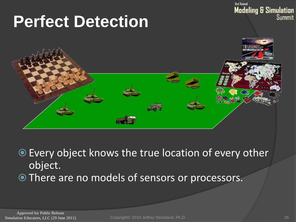
Perfect Detection

26

Every object knows the true location of every other object.

There are no models of sensors or processors.






Gridded Probability Areas

27

Perfect detection within the same grid area

• (Pdet = 1.0)

Probability of detection within adjacent areas

• Adjacent Pdet =F(terrain)

• Non-Adjacent Pdet = 0.0

60%

30%

100%

0%






Detection Range

28

Complete circle—no field of view/field of regard Terrain line-of-sight (LOS) is separate






3D Detection Range

29

Probability of detection based on range of spheres

Concentric areas• Different Pdet for each ring

• For some sensors, Pdet of inner ring is 0.00

𝜓 = 𝜓0

sin𝜋𝑎𝜆sin 𝜃

𝜋𝑎𝜆sin 𝜃

sin𝑁2

2𝜋𝑑𝜆

sin 𝜃 + 𝜙

sin𝜋𝑑2sin 𝜃 + 𝜙

𝐼 = 𝐼0sin



2 sin𝑁2

2𝜋𝑑𝜆

sin 𝜃 + 𝜙

sin𝜋𝑑2sin 𝜃 + 𝜙

2




http://upload.wikimedia.org/wikipedia/commons/6/61/Radar_RAF_Fylingdales.jpg

http://upload.wikimedia.org/wikipedia/commons/6/61/Radar_RAF_Fylingdales.jpg



ALARM—Advanced Low Altitude Radar Model—4.2 ALARM is a generic digital computer simulation designed to evaluate the performance of a

ground based radar system attempting to detect low altitude aircraft. The purpose of ALARM is to provide a radar analyst with a software simulation tool to evaluate

the detection performance of a ground-based radar system against the target of interest in a realistic environment.

Used in EADSIM

ALARM can simulate pulsed/Moving Target Indicator (MTI) pulse Doppler (PD) type radar systems limited capability to model continuous

wave (CW) radar. Radar detection calculations are based on the

signal-to-noise (S/N) radar range equations commonly used in radar analysis.

ALARM has four simulation modes: Flight Path Analysis (FPA) mode, Horizontal Detection Contour (HDC) mode Vertical Coverage Envelope (VCE) mode Vertical Detection Contour (VDC) mode






Target Acquisition

Glimpse models

Intermittent glimpses: E[N] = Σn np(n)

Continuous looking model = PROBDETECT in time t = 1 - e-Dt

DYNTACS curve fit model = D = PFOV (α/(β + t(δ + ζR2 – ξVc)))

NVEOL acquisition algorithm

Factors

Sensor

characteristics

Target characteristics

Line-of-sight

31

Glance/

Glimpse

Target

Found?

No

Yes

tg tg tg

Pacq Pacq Pacq






NVEOL Acquisition Algorithm

32

Joint

Conflicts

And

Tactical

Simulation

Developed by US Army's Night Vision

and Electro-Optical Laboratories

In Time-Stepped Model:

PROBDETECT in time T = PINF (1 - e -CT)

Use this as success probability for a Bernoulli trial.

In Event-Stepped Model:

Compute PINF and draw a random number to determine if detection would occur in infinite amount of time

Sample from an exponential distribution with mean C to determine time till detection given that a detection will occur.




http://www.jtepforguard.com/gallery/jcats_album/images/jcats10_gif.gif

http://www.jtepforguard.com/gallery/jcats_album/images/jcats10_gif.gif

http://www.jtepforguard.com/gallery/

http://www.jtepforguard.com/gallery/



Line-of-Sight Models

EXPLICIT: combat model stores a terrain representation and uses it to compute line-of-sight Grid: covers the battlefield with regular polygonal grid, each grid having

associated terrain attributes (e.g., elevation, vegetation, etc.)○ Look at intervening grids between observer and target to see if any grid is higher than the

line between them.

○ Discontinuity is a disadvantage in high-res models.

○ Simplicity and speed are advantages.

Surface○ Triangulate the terrain data grids, then interpolate for a point between grid points.

○ Greater accuracy is an advantage in high-res models.

IMPLICIT: combat model stores expected results of line-of-sight and looks up the result when required probability of LOS

intervisibilty segment length

33

. . . . . . . . . . . . . . . . .Primary Direction of

view (white)

Max Range

of view

LOS does not

exist

LOS exists

Orange lines

Left Limit

of View (white)

Right Limit

of View (white)






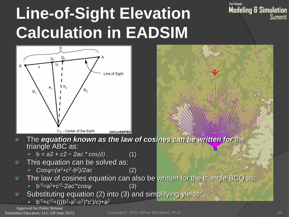
Line-of-Sight Elevation

Calculation in EADSIM

34

The equation known as the law of cosines can be written for the triangle ABC as: b = a2 + c2 − 2ac * cos(∂) . (1)

This equation can be solved as: Cosψ=(a2+c2-b2)/2ac (2)

The law of cosines equation can also be written for the triangle BCQ as: b’2=a2+c’2-2ac’*cosψ (3)

Substituting equation (2) into (3) and simplifying yields: b’2=c’2+(((b2-a2-c2)*c’)/c)+a2






Comms Model Effects

Perfect Communications

Direct Message Passing

Broadcast Messages

Virtual Cell Layout

Physics Modeling






Comms Model Effects

Information exchange process info

process data

Intelligence collection ISR sensors

target sensors

fire control sensors

Comms system overload network, sender, receiver

Interference environment, electronic

warfare

Time delay

36

Evaluate Target's Intent

Evaluate Target's Geometry

Recognize Target

Update Target's Knowledge

Notify Knowledge Processing

Activity Diagram: Process Info Use Case

Process Info

Get Data from Fire

Control Sensor

Get Data from

Target Sensor

Get Info from Data

Processing






Perfect Communications

37

Targets

~~~~~

Orders

~~~~~

Reports

~~~~~

Shared information, no representation of comms

Software-to-software message delivery






Direct Message Passing

Consult command

status

If sender and receiver

are alive, then pass

message.

If sender health is

degraded, add error to

target location.

38

… …






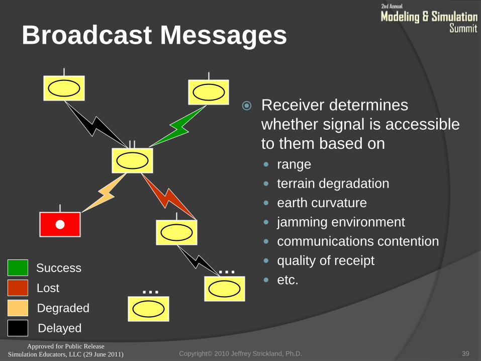
Broadcast Messages

Receiver determines

whether signal is accessible

to them based on

range

terrain degradation

earth curvature

jamming environment

communications contention

quality of receipt

etc.

39

……Success

Lost

Degraded

Delayed






Communications

Connectivity Modeling by

Propagation Network Types and their number of

participating platforms are as follows:

Duplex communication occurs in both

directions and is limited to two

participants.

Simplex communication occurs in

only one direction between two

participants. The first platform on list

is the transmitter.

Broadcast communication occurs

from one platform to several other

platforms. The first platform on the

list is the transmitter.

N-to-N serial communication occurs

between all the participant platforms.

N-Broadcast simultaneous

communication occurs between all

the participant platforms.

Land Line communication occurs

between two participants (not affected

by Jamming).

Links Exist if two Conditions are met:

Receiver signal power level must be

equal to or greater than user-specified

minimum discernible signal level

Signal-to-noise level (received signal

power level received jam power level)

must be equal to or greater than user-

specified signal-to-noise threshold






Point System

Markov Pk Tables

Random Numbers

Pk’s and Random Numbers

Precision Engagements

Linear Target Phit

Rectangular Target Phit

Circular Target Phit

Kill Categories






Point System

42

New Health = (Health + Armor) – (Weapon Power – Path Degrade)

New Health = (18 + 8) – (20 – 4) = 10

New Armor = Armor – ABS[( Weapon Power – Path Degrade) *0.25]

18

4

20

8

Weapon Power

Path Degradation(range, shelters, obstructions)

Health

Armor






Markov Pk Table

43

Pk

Weapon

W1 W2 W3 W4 …

T1 0.5 0.7 0.8 0.92

T2 0.4 0.45 0.76 0.99

T3 0.31 0.34 0.56 0.85

T4 0.27 0.55 0.67 0.81

Ta

rge

t

…

Phit is rolled into the overall Pkill

Damage = 1, where Random Number <= Pk

= 0, where Random Number > Pk






Random Numbers

44

0.002589 0.709121 0.688907 0.23241 0.248291 0.279792 0.099733

0.672374 0.177176 0.5124 0.253238 0.885889 0.08127 0.337699

0.967582 0.11894 0.917944 0.691778 0.377643 0.167685 0.23337

0.821207 0.775446 0.94055 0.916313 0.342373 0.494679 0.83171

0.76565 0.300179 0.081692 0.212297 0.323383 0.088898 0.976731

0.826355 0.633324 0.390983 0.559808 0.032313 0.337002 0.429531

0.284963 0.978167 0.177686 0.39425 0.729517 0.196937 0.053272

0.537055 0.753125 0.189256 0.790979 0.437795 0.757163 0.953741

0.714325 0.899821 0.139968 0.139168 0.803138 0.274158 0.226658

0.151101 0.555232 0.533085 0.327454 0.753654 0.268759 0.307099

0.21175 0.644434 0.011707 0.809213 0.3742 0.38085 0.412449

0.425525 0.346873 0.490443 0.397201 0.114504 0.831309 0.291209

0.157902 0.994106 0.22623 0.215775 0.503133 0.544428 0.05825

0.173804 0.322742 0.984154 0.512732 0.340096 0.626067 0.746717

0.391907 0.168648 0.606554 0.280939 0.804009 0.290058 0.550802

0.743599 0.108666 0.557355 0.850634 0.908114 0.209818 0.600702

0.682586 0.265387 0.792137 0.241523 0.077536 0.282332 0.244388

0.688018 0.607142 0.296545 0.583956 0.652407 0.773843 0.801856

0.037354 0.516678 0.27669 0.360097 0.700107 0.821834 0.912564

0.914889 0.18311 0.164431 0.880446 0.527801 0.887302 0.209683

Generated by a recursive function

Evenly distributed between 0 and 1 ~ Unif(0,1)

Perfect for Pk evaluations






Pk’s and Random Numbers

45

Kill Area No-Kill Area

0% 75% 100%

Random Number = 0.63

Pk = 75% = 0.75






Precision Engagements

46

Round Impact Point

PROBLEM: Find point of impact (if any) of round on its target.

ASSUMPTION: The projectile impact point is a random variable with a

normal probability distribution (empirically shown to be a good assumption).

Actual Target Location

Doctrinal Aim Point

Aim Point

“Bias” : Systematic Errors

“Dispersion” : Round-to-Round

Independent Errors

Perceived Doctrinal

Aim Point

Perceived Target Location






Linear Target Phit

47

Normal parameters for 1D target:• “Front view" (i.e., direct-fire weapon)

○ Deflection error

• "Top view" (i.e., indirect-fire weapon)○ Range error

• DEFINE:○ Bias = μ

○ Dispersion = σ

Error Probable - distance in deflection (for x) within

which half of rounds will land.

Linear Error Probable (LEP) - linear distance from aim

point within which half of rounds will land, based on the

error probable (details to follow).

x

p(x)

25 m






Single-Shot Accuracy1D Target Example 1

Assume no systematic error.

48

2126.03937.06063.0 zzPSSH

NOTE: “” is available in

tabular form in any Statistics

text: see Normal Distribution.

3937.00644.37010

6064.00644.37010

then,m, 10 m, 0664.376745.025 0,

z

z

x

PSSH

0

-z +z






Rectangular Target Phit

Normal parameters for 2D target: "Side view" (i.e., direct-fire weapon)

○ Elevation error


"Top view" (i.e., indirect-fire weapon)○ Range error


DEFINE: Bias = μx , μy

Dispersion = σx , σy

Range Error Probable (REP) – linear distance from aim point within which half of rounds will land, x-coordinate

Cross-range Error Probable (CREP) – linear distance from aim point within which half of rounds will land, y-coordinate

49

x

y

p(y)

p(x)






Circular Target Phit

P(destruction of a point target) = P(hit within a circle of radius

R), i.e., Pd = P.

When x0 = y0 = 0 and x2 = y2 = 2,

If R0 is the radius of a circle for which

then 50% of all impacts points for the probability distribution P(r) will fall

within this radius r ≤ R0.

R0 is called the circular error probable (CEP), and R0 =

1.1774.

50

2

2

2exp1

RRPd

2

1

2exp1

2

2

00

RRP

Target

Simplified Vehicle

Assembly Area

Cluster of Soldiers






Kill CategoriesK-Kill: catastrophic kill

F-Kill: firepower kill

M-Kill: mobility kill

MF-Kill: mobility & firepower kill, usually => K-Kill

P-Kill: personnel kill (crew and passengers)

No-Kill: no damage due to hit.

51

ranx = random(seed)

if (ranx < PkN)

{No Kill}

else if (ranx < PkN + PkM)

{Mobility Kill}

else if (ranx < PkN + PkM + PkF)

{Firepower Kill}

else if (ranx < PkN + PkM + PkF + PkMF)

{Mobility & Firepower Kill}

else

{Catastrophic Kill}

Single random number draw can result

in more than just “Miss/Hit”

Engagement outcome has at least 5

states






Direct-Fire Accuracy Example (1)

An infantry fighting vehicle (IFV) has the following frontal profile:

A hit in area 1 will

produce a firepower kill.


produce a catastrophic kill.


produce a mobility kill.

A hit in other areas will

produce no permanent effect.

Assess the IFV’s vulnerability when engaged with a frontal shot whose impact point is modeled as a random variable pair (X,Y) ~ BVN(0,0,.5,.5,0).

Using the below list of pseudo random numbers as needed, simulate the first round to determine which type of kill, if any, occurs (.8554, .2287, .6659, .8243, .6840, .0430, .8598, .2381, .5035, .2723).

52

2

1 44

3

0.6

1.6

1.0

1.4 2.6

0.6






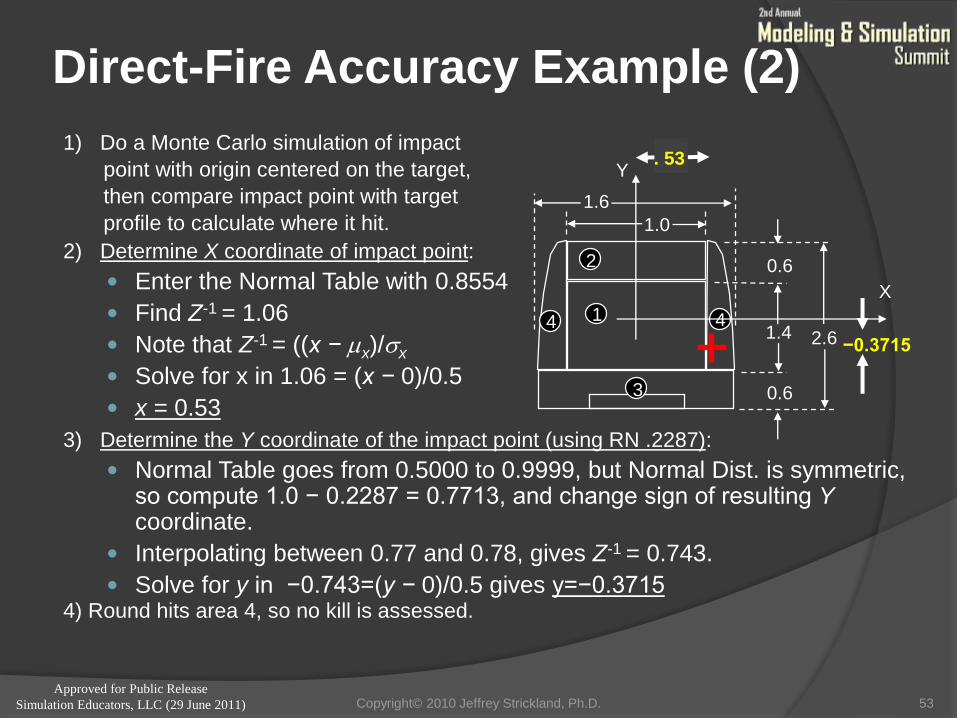
Direct-Fire Accuracy Example (2)

1) Do a Monte Carlo simulation of impact

point with origin centered on the target,

then compare impact point with target

profile to calculate where it hit.

2) Determine X coordinate of impact point:

Enter the Normal Table with 0.8554

Find Z-1 = 1.06

Note that Z-1 = ((x − x)/x

Solve for x in 1.06 = (x − 0)/0.5

x = 0.53

3) Determine the Y coordinate of the impact point (using RN .2287):

Normal Table goes from 0.5000 to 0.9999, but Normal Dist. is symmetric, so compute 1.0 − 0.2287 = 0.7713, and change sign of resulting Ycoordinate.

Interpolating between 0.77 and 0.78, gives Z-1 = 0.743.

Solve for y in −0.743=(y − 0)/0.5 gives y=−0.37154) Round hits area 4, so no kill is assessed.

53

2

1 44

3

0.6

1.6

1.0

1.4 2.6

0.6

Y

X

−0.3715

. 53






Lanchester Equations

Aggregated Combat Groups

Epstein’s Equations

Quantified Judgment Model (QJM)

Force Ratio Approach






Lanchester Equations

dx

dtf x y

dy

dtf x y 1 2, ,... , ,...

55

CONCEPT: describe the rate at which a force loses

systems as a function of the size of the force and

the size of the enemy force. This results in a system

of differential equations in force sizes x and y.

The solution to these equations as functions of x(t)

and y(t) provide insights about battle outcome.

aydt

dx

bxdt

dy






Aggregated Combat Groups

Contiguous

pistons

Aggregated force

attrition

Distance from

middle affects

power and attrition

Units accumulate

as piston moves

Explicit withdrawal

required






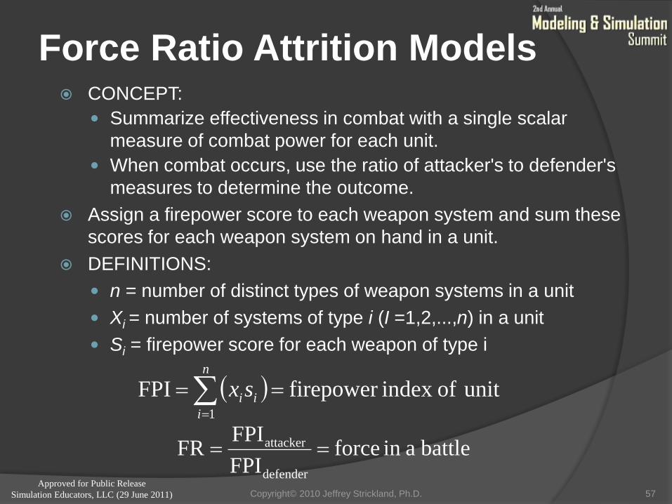
Force Ratio Attrition Models CONCEPT:

Summarize effectiveness in combat with a single scalar

measure of combat power for each unit.

When combat occurs, use the ratio of attacker's to defender's

measures to determine the outcome.

Assign a firepower score to each weapon system and sum these

scores for each weapon system on hand in a unit.

DEFINITIONS:

n = number of distinct types of weapon systems in a unit

Xi = number of systems of type i (I =1,2,...,n) in a unit

Si = firepower score for each weapon of type i

57

unit ofindex firepower FPI1

n

i

iisx

battle ain forceFPI

FPIFR

defender

attacker






Other Aggregated Models

Epstein equations

Defender’s withdrawal rate:

Attacker’s Prosecution rate:

Quantified Judgment Model (QJM) T.N. Dupuy created the QJM to transform Clausewitz’s Law of Number to

a combat power formula.

Multi-agent models The environment takes the form of a distributed network of place agents.

Aggregate state-space models Represented by aggregate state variables, rather than the locations and

current behaviors of individual entities

58

aTa

aT

gaT

gg

dTd

dT

tt

tt

ttWW

tWtW

11

1

11

11 max






Missile Dynamics

Sensor Dynamics

Coordinate Systems

Missile Flight Simulation






Components of Missile Flight

Simulation

MISSILE SYSTEM DESCRIPTION

MISSILE

GUIDANCE

LAUNCHER

MISSILE DYNAMICS

MISSILE AERODYNAMICS

MISSILE PROPULSION

MISSILE AND TARGET MOTION

GUIDANCE AND CONTROL MODELING

SCENE SIMULATION

IMPLEMENTATION






Missile Dynamics

Axis

Force

Along

Axis

Moment

About

Axis

Linear

Velocity

Angular

Displacement

Angular

Velocity

Moment

of Inertia

𝑥 𝐹𝑥 𝐿 𝑢 𝜙 𝑝 𝐼𝑥

𝑦 𝐹𝑦 𝑀 𝑣 𝜃 𝑞 𝐼𝑦

𝑥 𝐹𝑧 𝑁 𝑤 𝜓 𝑟 𝐼𝑧

61

𝑀, 𝑞

𝑦𝑏

𝑥𝑏

𝑧𝑏

𝑁, 𝑟

𝐿, 𝑝

𝐹𝑥, 𝑢

𝐹𝑦, 𝑣

𝐹𝑧, 𝑤

𝑢 =𝐹𝑥𝑏𝑚

− 𝑞𝑤 − 𝑟𝑣 , m/s2

𝑣 =𝐹𝑦𝑏𝑚

− 𝑟𝑢 − 𝑝𝑤 , m/s2

𝑤 =𝐹𝑧𝑏𝑚

− 𝑝𝑣 − 𝑞𝑢 , m/s2

𝑝 = 𝐿 − 𝑞𝑟 𝐼𝑧 − 𝐼𝑦 𝐼𝑥 , m/s2

𝑞 = 𝑀 − 𝑝𝑟 𝐼𝑥 − 𝐼𝑧 𝐼𝑦 , m/s2

𝑟 = 𝑁 − 𝑝𝑞 𝐼𝑦 − 𝐼𝑥 𝐼𝑧 , m/s2

ROTATIONAL EQUATIONS

TRANSLATIONAL EQUATIONS




Sensor Dynamics

Pseudo-imaging

Imaging

Radio Frequency

Seekers

Pulse Radar

Continuous Wave

Radar

Pulse Doppler Radar




Projection of Tracking

Error on Reticle Plane

63

BoresightAxis

AngularTracking Error

Tracking Error Vector

Field of View

Plane of ReticleDetector

ArbitraryReference

Target Projection on Reticle

Line ofSight

Target






Coordinate Systems

64

Target Coordinate System (𝑥𝑡, 𝑦𝑡, 𝑧𝑡)

Body Coordinate System (𝑥𝑏, 𝑦𝑏 , 𝑧𝑒)

Earth Coordinate System (𝑥𝑒 , 𝑦𝑒 , 𝑧𝑒)

Guidance Coordinate System (𝑥𝑔, 𝑦𝑔, 𝑧𝑔)

Tracker Coordinate System (𝑥𝑠, 𝑦𝑠, 𝑧𝑠)

Wind Coordinate System (𝑥𝑤, 𝑦𝑤, 𝑧𝑤)






Missile Simulation

65

𝑋 1 = 𝑃𝑀 𝑖

𝑋 2 = 𝑃𝑀 𝑗

𝑋 3 = 𝑃𝑀 𝑖𝑘

𝑋 4 = 𝑢𝑋 5 = 𝑣𝑋 6 = 𝑤𝑋 7 = 𝑢𝑋 8 = 𝑣𝑋(9) = 𝑤

Read and Initialize

Input Data

Atmosphere,

Mach Number,

Dynamic Pressure

Relative Velocity,

Range,

Range Rate

Closest

Approach

?

Guidance and Control

Forces on Missile

Missile Accelerations

Update Missile and Target

Positions and Velocities

Update Time, Missile

Mass, CM Location, and

Moments of Inertia

T > Tmax

Or

Crash?

End

Miss Distance

Yes

YesNo

No

𝑃𝑀 𝑖 = 𝑋𝑂𝑈𝑇 1

𝑃𝑀 𝑗 = 𝑋𝑂𝑈𝑇 2

𝑃𝑀 𝑘 = 𝑋𝑂𝑈𝑇 3

𝑢 = 𝑋𝑂𝑈𝑇 4𝑣 = 𝑋𝑂𝑈𝑇 5𝑤 = 𝑋𝑂𝑈𝑇 6 𝑢 = 𝑋𝑂𝑈𝑇 7 𝑣 = 𝑋𝑂𝑈𝑇 8 𝑤 = 𝑋𝑂𝑈𝑇(9)






FlatEarthMissileEqns(u)% Define Control Variables from Inputs

T = u(1); % thrust along missile velocity

wel = u(2); % turn rate in elevation

waz = u(3); % turn rate in azimuth

% Define State Variables from Inputs

x = u(4:12);

% Location Variables

Px = x(1); % Position in Direction of North Pole

Py = x(4); % Position At Equator in y

Pz = x(7); % Position At Equator in z

% Body_Axes Velocities

U = x(2); % velocity in Px direction

V = x(5); % velocity in Py direction

W = x(8); % velocity in Pz direction ("Up")

% Body Axes Acceleration

%Accx = x(3);

%Accy = x(6);

%Accz = x(9);

% Speed, Atmospheric Density and Drag

Vxy2 = U^2 + V^2;

Vxy = sqrt(Vxy2);

Vxz2 = U^2 + W^2;

Vt2 = Vxz2 + V^2;

Vt = sqrt(Vt2);

az = atan2(V, U);

el = atan2(W, Vxy);%

Atmospheric Density in kg/meterA3

if Pz < 0 % Travel inside the Earth is Viscous

rho = 10^2;

elseif Pz < 9144 % Altitudes below 9144 meters

rho = 1.22557*exp(-Pz/9144);

else % Altitudes above 9144 meters

rho = 1.75228763*exp(-Pz/6705.6);

end

beta = cfric*rho;

Tacc = T/Vt;

% Compute the Derivatives

dPx = U;

dPy = V;

dPz = W;






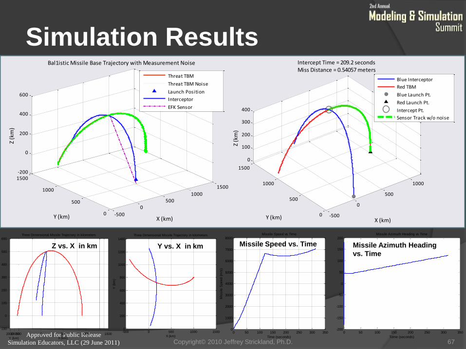
Simulation Results

67

-500 0 500 1000 1500010002000

-100

0

100

200

300

400

500

600

X (km)

Three Dimensional Missile Trajectory in kilometers

Y (km)

Z (

km

)

-500 0 500 1000 15000

200

400

600

800

1000

1200

1400

X (km)

Three Dimensional Missile Trajectory in kilometers

Y (

km

)

0 50 100 150 200 250 300 3500

1000

2000

3000

4000

5000

6000

7000

8000

Mis

sile

Speed (

m/s

)

Time (seconds)

Missile Speed vs Time

0 50 100 150 200 250 300 350-200

-150

-100

-50

0

50

100

150

200Missile Azimuth Heading vs Time

Tome (seconds)

Missile Azimuth Heading

vs. Time

Missile Speed vs. TimeY vs. X in kmZ vs. X in km

-500

0

500

1000

0

500

1000

1500

0

100

200

300

400

X (km)

Intercept Time = 209.2 secondsMiss Distance = 0.54057 meters

Y (km)

Z (k

m)

Blue Interceptor

Red TBM

Blue Launch Pt.

Red Launch Pt.

Intercept Pt.

Sensor Track w/o noise

-500

0500

1000

1500

0

500

1000

1500-200

0

200

400

600

X (km)

Bal1istic Missile Base Trajectory with Measurement Noise

Y (km)

Z (k

m)

Threat TBM

Threat TBM Noise

Launch Position

Interceptor

EFK Sensor






Elements of a Scenario

Scenario Development

Scenario Generation Tools






Elements of a Scenario Settings

environment, terrain, etc.

Actors

Blue/Red forces, weapons, sensors, etc.

Task Goals

missions, objectives, etc.

Plans

overlays, control measures, etc.

Actions

move, shoot, communicate, etc.

Events

contact, engagements, etc.






Scenario Considerations

Resolution (high or low)

Aggregated-disaggregated

Terrain data

Weapon/Sensor data

Virtual or constructive

Interfaces

Distributed/federated






Scenarios in EADSIM

71

ELEMENT DATA

LAYDOWN

SCENARIOS

PLATFORMPLATFORMPLATFORMPLATFORMNETWORKS

ROUTES

AOIs

MAP

ENVIRON

OBJECT REF

PROTOCOLS

SYSTEMS

WEAPONS

EMP

COMM DEV

JAMMERS

SENSORS

RULESETS

MANEUVERS

FORMATIONS

PP TABLES

FLYOUT TABLES

PK TABLES

ICONS

IR SIG

RADAR SIG

AIRFRAMES

SPECIFICATION OF A SCENARIO

SCENARIOS ARE THEN A

FURTHER COMBINATION

OF LOWER LEVEL DATA

SYSTEMS ARE DEPLOYED

ELEMENTS

COMBINE TO MAKE

SYSTEM ELEMENTS

INDIVIDUAL

COMPONENTS ARE

SPECIFIED AS

ELEMENTS





Simulation Educators, LLC (29 June 2011) 72

Provide users the ability to:

• Create, modify, and verify

scenario files.

• Specify entities,

tactical overlays,

and environment

parameters.

Scenario Generation Tools are typically developed to be utilized as an off-line pre-runtime tool that can be run on a laptop and provide a modular scenario development environment

Ability to translate legacy scenario files

into the new scenario file format & able to

translate the new scenario files back into

the legacy format

Simulation

System

Scenario Generation Tools (SGTs)






Summary

The are several types of combat models driving simulations for combat training, research & development, and advanced concepts requirements:

Environmental models

Physical models (engagement, target acquisition, communications, etc.)

Behavioral models

In addition, simulations require some means of scenario development, and these are often separate components.

Understanding the underlying concepts and methods of combat models embedded in simulations, enhances our ability to choose the right simulations for our training or analysis requirements.






ReferencesAncker, C.J., Jr. and Gafarian, A.V., Modern Combat Models: A Critique of Their Foundations, Operations Research

Society of America, 1992.

Bracken, J., Kress, M. and Rosenthal, R.E., Eds., Warfare Modeling, MORS, 1995.

Caldwell, B, Hartman, J., Parry, S., Washburn, A., and Youngren, M., Aggregated Combat Models. NPS ORD, 2000.

Davis, P.K., Aggregation, Disaggregation, and the 3:1 Rule in Ground Combat. MR-638

DuBois, E.L., Hughes, W.P., Jr., Low, L.J., A Concise Theory of Combat, Institute for Joint Warfare Analysis, NPS, 2000.

Dupuy, T.N., Understanding War: History and Theory of Combat, Falls Church, VA.: Nova 1987.

Epstein, J.M., The Calculus of Conventional War: Dynamic Analysis without Lanchester Theory, Washington, D.C., Brookings Institute, 1985.

Fowler, B.W., De Physica Beli: An Introduction to Lanchestrial Attrition Mechanics, 3 Vols. IIT Research Institute/DMSTTIAC, Rept. SOAR 96-03, Sep. 1996.

Hillestad, R.J., and Moore, L., The Theater-Level Campaign Model: A New Research Prototype for a New Generation of Combat Analysis Model, RAND, 1996. MR-388

Koopman, B.O., Search and Screening, MORS, 1999.

Reece, D.A., Movement behavior for soldier agents on a virtual battlefield, Teleoperators and Virtual Environments , Volume 12 , Issue 4 (August 2003). MIT Press Cambridge, MA, USA

Smith, R. Military Simulation, http://www.modelbenders.com/

Strickland, J. S. Missile Fight Simulation. Lulu.com, 2011.

Strickland, J. S. Using Math to Defeat the Enemy. Lulu.com, 2011.

Strickland, J. S., Fundamentals of Combat Modeling, Lulu.com, 2010.

Taylor, J.G., Lanchester Models of Warfare, 2 Vols, Defense Technological Information Center (DTIC), ADA090843 (Naval Post Graduate School, Monterey, CA), October 1980.

Taylor, J.G., Force-on-Force Attrition Modeling, Operations Research Society of America, Military Applications Section, 1981.

Washburn, A.R., Search and Detection, 4th Ed., Operations Research Section, INFORMS, Baltimore, MD, 2002.

Washburn, A., Lanchester Systems, NPS, April 2000.




Engineering

Using math to defeat the enemy (7 7-2011)