Download pdf - A Triaxial Accelerometer Calibration Method Using a Mathematical Model

2144 IEEE TRANSACTIONS ON INSTRUMENTATION AND MEASUREMENT, VOL. 59, NO. 8, AUGUST 2010

A Triaxial Accelerometer Calibration MethodUsing a Mathematical Model

Seong-hoon Peter Won and Farid Golnaraghi

Abstract—This paper presents a new triaxial accelerometercalibration method using a mathematical model of six calibrationparameters: three gain factors and three biases. The fundamentalprinciple of the proposed calibration method is that the sum of thetriaxial accelerometer outputs is equal to the gravity vector whenthe accelerometer is stationary. The proposed method requires thetriaxial accelerometer to be placed in six different tilt angles to esti-mate the six calibration parameters. Since the mathematical modelof the calibration parameters is nonlinear, an iterative method isused. The results are verified via simulations by comparing theestimated gain factors and biases with the true gain factors andbiases. The simulation results confirm that the proposed method isapplicable in extreme cases where the gain factor is 1000 V/(m/s2)and the bias is ±100 V, as well as the cases where the gain factoris 0.001 V/(m/s2) and the bias is 0 V. The proposed calibrationmethod is also experimentally tested with two different triaxialaccelerometers, and the results are validated using a mechanicalinclinometer. The experimental results show that the proposedmethod can accurately estimate gain factors and biases even whenthe initial guesses are not close to the true values. In addition,the proposed method has a low computational cost because thecalculation is simple, and the iterative method usually convergeswithin three iteration steps. The error sources of the experimentsare discussed in this paper.

Index Terms—Acceleration measurement, calibration, gravitymeasurement, iterative method, parameter estimation.

I. INTRODUCTION

T RIAXIAL accelerometers are used in various applica-tions, such as inertial navigation systems (INSs) [1], [2]

and inclinometers [3]–[5]. Such accelerometers must be cali-brated as accurately as possible because accelerometers witheven small biases could result in a very fast position driftwhen they are used for INS applications [6] and could resultin inaccurate tilt angle measurements. Since the calibrationparameters of a triaxial accelerometer vary under differentenvironmental conditions [7], including temperature change[8], the gain factors and biases change whenever the sensoris switched on. Thus, an accelerometer must be calibratedbefore use or when the temperature is significantly changed.

Manuscript received March 9, 2009; revised July 11, 2009; acceptedAugust 3, 2009. Date of publication October 23, 2009; date of current versionJuly 14, 2010. The Associate Editor coordinating the review process for thispaper was Dr. Jiong Tang.

S. P. Won is with the Department of Mechanical Engineering, University ofWaterloo, Waterloo, ON N2L 3G1, Canada (e-mail: [email protected]).

F. Golnaraghi is with the Mechatronic System Engineering, Simon FraserUniversity, Surrey, BC V3T 0A3, Canada (e-mail: [email protected]).

Color versions of one or more of the figures in this paper are available onlineat http://ieeexplore.ieee.org.

Digital Object Identifier 10.1109/TIM.2009.2031849

To frequently calibrate a triaxial accelerometer, the calibrationmethod should have a simple procedure. In the past, differentattempts have been reported in the literature to calibrate triaxialaccelerometers.

The conventional method of a triaxial accelerometer calibra-tion involves rotating an accelerometer at known tilt angles[9]–[11]. To achieve accurate results with this method, thetilt angles must precisely be measured. Calibration methodsusing an external device, such as actuator [12], [13] or positionsensor [14], [15], can accurately compute the gain factors andbiases, but such device is not usually available outside of alaboratory. Accelerometer calibration techniques that do notrequire precise tilt angle measurements or an external deviceare presented in [3] and [16]–[20]. The methods in [16] and[17] use least-square estimation to calculate gain factors, biases,and misalignment errors. The method of least squares allowsredundant tilt angle measurements to achieve more accuratecalibration results. However, Syed et al. [17] stated that theinitial estimations of gain factors and biases should be closeto the true values to converge to reasonable gain factors andbiases to use the method in [16]. To find the rough estimates ofgain factors and biases, the method in [17] includes a calibrationprocedure step of roughly aligning the three axes of the sensorwith the gravity vector once positively and once negatively.Calibration methods that rely on the Taylor series expansion upto the first-order term to linearize the nonlinear mathematicalmodel of the gain factors and biases are presented in [18]–[20].Lai et al. [18] described a method to find three gain factorsand three biases of a triaxial accelerometer by placing it in sixdifferent randomly chosen tilt angles in a stationary state. Thismethod usually requires five iterative steps to estimate the gainfactors and biases. Lai et al. [18] stated that this method alsorequires the initial estimations of the gain factors and biasesto be close to the true values not to diverge from the correctsolution.

This paper presents a novel triaxial accelerometer calibrationmethod that has a very simple procedure with a high accuracy.The proposed triaxial accelerometer calibration method utilizesthe gravity vector and the mathematical model of the calibrationparameters. This method only requires the triaxial accelerome-ter to be stationary in six different tilt angles to estimate sixcalibration parameters and does not require any knowledge ofthe tilt angles. The simulation and experiment results show thatthe gain factors and biases did not diverge although the initialguesses were not close to the true values. In addition, the resultsshow that the proposed method can estimate gain factors andbiases within three iteration steps.

0018-9456/$26.00 © 2009 IEEE

WON AND GOLNARAGHI: TRIAXIAL ACCELEROMETER CALIBRATION METHOD USING A MATHEMATICAL MODEL 2145

Fig. 1. Flowchart diagram of the proposed triaxial accelerometer calibration method.

Fig. 2. Calibration procedure: the proposed calibration method requires six different tilt angle measurements to determine six calibration parameters.

II. CALIBRATION USING AN ITERATIVE METHOD

Fig. 1 summarizes the calibration parameter estimation stepsand the process of conversion from the triaxial accelerometerdata to accelerations. If the calibration parameters are available,then the accelerometer data are converted from voltage to accel-eration; but if the calibration parameters are not available, thenthe proposed method outputs the accelerometer measurements.The fundamental concept of the proposed triaxial accelerometercalibration method is that the vector sum of accelerations mea-sured with a triaxial accelerometer is equal to the gravity vectorwhen the sensor is stationary. Since a triaxial accelerometer hassix unknown calibration parameters, it has to be placed in sixdifferent stationary tilt angles to obtain six equations (Fig. 2).When six tilt angles are collected, six calibration parameterscan be estimated from the derived equations.

When the sensor is stationary, the relationship between thelocal gravity vector (1g) and the accelerations in the X-, Y -,and Z-axes (AX , AY , and AZ , respectively) is

A2X + A2

Y + A2Z = (1g)2. (1)

The relationship between the accelerometer outputs in each axis(Saxis) and the true acceleration in each axis (Aaxis) can bewritten as

Saxis = Gaxis · Aaxis + Baxis (2)

where Gaxis is the true gain factor of each axis, and Baxis is thetrue bias of each axis.

The proposed calibration method uses an iterative method tocalculate the gain factors and biases of each axis of a triaxial

accelerometer. To implement an iterative method, (2) should berewritten so that it fits the method. Thus, (2) is rewritten as

Saxis =Gaxis · Aaxis + Baxis

=

(k∏

i=0

Gaxis,i

)· Aaxis,k +

k∑i=0

Baxis,i

= Gaxis,k · Aaxis,k + Baxis,k (3)

where Gaxis,i represents the calculated gain factor of each axisat the ith iteration, Baxis,i represents the calculated bias of eachaxis at the ith iteration, Aaxis,k is the estimated acceleration ofeach axis at the kth iteration, Gaxis,k is the estimated gain factorof each axis at the kth iteration, and Baxis,k is the estimated biasof each axis at the kth iteration. Given that the true gain factorsare real positive numbers and the true biases are real numbers,the initial estimated gain factor of each axis (Gaxis,0) can bechosen from any positive real number, and the initial estimatedbias of each axis (Baxis,0) can be chosen from any real number.

When the iterative method converges, the estimated gainfactors and biases at the kth iteration should match their truecounterparts. Thus, the objective of the iterative method is todetermine the calculated gain factors of each axis (Gaxis,k) andthe calculated biases of each axis (Baxis,k) that satisfy

Gaxis = Gaxis,k = Gaxis,k−1 · Gaxis,k

Baxis = Baxis,k = Baxis,k−1 + Baxis,k. (4)

From (3), the estimated acceleration at the (k − 1)thiteration is

Aaxis,k−1 = (Saxis − Baxis,k−1)/Gaxis,k−1. (5)


Since the accelerometer outputs are known as well as theprevious estimated gain factors and biases, the acceleration ofeach axis at the (k − 1)th iteration can be calculated using (5).When the accelerometer is stationary, (1) holds. If Aaxis,k−1

does not match the true acceleration of each axis (Aaxis), anerror is encountered. The error term at the (k − 1)th iteration is

Ek−1 = (AX,k−1)2 + (AY,k−1)2 + (AZ,k−1)2 − 1g2

=((SX − BX,k−1)/GX,k−1

)2

+((SY − BY,k−1)/GY,k−1

)2

+((SZ − BZ,k−1)/GZ,k−1

)2

− 1g2. (6)

Since all the terms in (6) are known, Ek−1 can be calculated.By using (1), (6) can also be written as

Ek−1 =((SX − BX,k−1)/GX,k−1

)2

+((SY − BY,k−1)/GY,k−1

)2

+((SZ − BZ,k−1)/GZ,k−1

)2

−(A2

X + A2Y + A2

Z

). (7)

The acceleration terms in (7) are replaced with the knownaccelerometer terms from (3) and (4). Then, (7) can beexpanded as

Ek−1 =(1 − 1/G2

X,k

)· A2

X,k−1

+ 2 · BX,k · AX,k−1/(GX,k−1 · G2

X,k

)+

(1 − 1/G2

Y,k

)· A2

Y,k−1

+ 2 · BY,k · AY,k−1/(GY,k−1 · G2

Y,k

)+

(1 − 1/G2

Z,k

)· A2

Z,k−1

+ 2 · BZ,k · AZ,k−1/(GZ,k−1 · G2

Z,k

)− εk−1 (8)

where

εk−1 = B2X,k/(GX,k−1 · GX,k)2 + B2

Y,k/(GY,k−1 · GY,k)2

+ B2Z,k/(GZ,k−1 · GZ,k)2.

Equation (8) has six unknowns, and the last term εk−1 isnonlinear with all six unknowns. However, when the iterationsconverge, εk−1 becomes almost zero because the calculatedbias terms (BX,k, BY,k, and BZ,k) are expected to convergeto zero. By setting εk−1 to zero, (8) can be rewritten as

Ek−1 =(1 − 1/G2

X,k

)· A2

X,k−1

+ 2 · BX,k · AX,k−1/(GX,k−1 · G2

X,k

)

+(1 − 1/G2

Y,k

)· A2

Y,k−1

+ 2 · BY,k · AY,k−1/(GY,k−1 · G2

Y,k

)

+(1 − 1/G2

Z,k

)· A2

Z,k−1

+ 2 · BZ,k · AZ,k−1/(GZ,k−1 · G2

Z,k

). (9)

To solve for the six calibration parameters, a triaxial accelerom-eter should be placed in six different tilt angles. Then, (9)becomes a 6 × 1 matrix such that we have (10), shown at thebottom of the page. Matrix [Errork−1] can be calculated from(6), and matrix [Accelk−1] can be calculated from (5). Sincematrix [Errork−1] and matrix [Accelk−1] are known, matrix[Calk] is calculated as

[Calk] = [Accelk−1]−1 · [Errork−1]. (11)

From Matrix [Calk], three calculated gain factors at the kthiteration should first be determined from the first three rows.Then, using the square of the calculated gain factors at thekth iteration and the estimated gain factors at the (k − 1)thiteration, three calculated biases at the kth iteration can bedetermined from the last three rows. The gain factors, however,

[Errork−1] = [Accelk−1] · [Calk]

⎡⎢⎢⎢⎢⎢⎣

Ek−11Ek−12Ek−13Ek−14Ek−15Ek−16

⎤⎥⎥⎥⎥⎥⎦ =

⎡⎢⎢⎢⎢⎢⎢⎣

AX,k−112 AY,k−112 AZ,k−112 AX,k−11 AY,k−11 AZ,k−11AX,k−122 AY,k−122 AZ,k−122 AX,k−12 AY,k−12 AZ,k−12AX,k−132 AY,k−132 AZ,k−132 AX,k−13 AY,k−13 AZ,k−13AX,k−142 AY,k−142 AZ,k−142 AX,k−14 AY,k−14 AZ,k−14AX,k−152 AY,k−152 AZ,k−152 AX,k−15 AY,k−15 AZ,k−15AX,k−162 AY,k−162 AZ,k−162 AX,k−16 AY,k−16 AZ,k−16

⎤⎥⎥⎥⎥⎥⎥⎦·

⎡⎢⎢⎢⎢⎢⎢⎢⎢⎢⎢⎣

1 − 1/G2X,k

1 − 1/G2Y,k

1 − 1/G2Z,k

2 · BX,k/(GX,k−1 · G2

X,k

)2 · BY,k/

(GY,k−1 · G2

Y,k

)2 · BZ,k/

(GZ,k−1 · G2

Z,k

)

⎤⎥⎥⎥⎥⎥⎥⎥⎥⎥⎥⎦(10)


TABLE ISIMULATION RESULTS WITH DIFFERENT GAIN FACTORS AND BIASES

Fig. 3. Tilt angle contents of the simulations: tilt angles for (a) Simulation 1, (b) Simulation 2, (c) Simulation 3, (d) Simulation 4, and (e) Simulation 5.

have to be real positive numbers. To ensure that the calculatedgain factors are positive real numbers, they are calculated as

GX,k =∣∣∣1 − ([Accelk−1]

−1 · [Errork−1])1∣∣∣−0.5

,

GY,k =∣∣∣1 − ([Accelk−1]

−1 · [Errork−1])2∣∣∣−0.5

,

GZ,k =∣∣∣1 − ([Accelk−1]

−1 · [Errork−1])3∣∣∣−0.5

, (12)

where subscripts 1, 2, and 3 represent the row number of[Accelk−1]−1 · [Errork−1] matrix.

After the six unknowns are determined, the estimated gainfactors and biases at the kth iteration can be obtained from(4). This iterative method terminates when the three calculatedgain factors converge to unity and the three calculated biasesconverge to zero.

III. SIMULATIONS

In the experiments, it is difficult to validate the calibrationresults because the true gain factors and biases are unknown.Thus, simulations are used to validate the proposed calibrationmethod. The true gain factors and biases are defined for thesimulation, and the accelerometer data are generated usingMATLAB based on true gain factors, true biases, gravity, andmovement of the accelerometer. Then, by using the proposedcalibration method, gain factors and biases are estimated. Unity

gain factors and zero biases are used to initialize the iterativealgorithm. When the final estimated gain factors and biasesare calculated using the proposed calibration method, they arecompared with the true gain factors and biases.

One hundred simulations were performed with gain fac-tors between 0.001 and 1000 [V/(m/s2)] and biases between±100 V. The six stationary tilt angles had at least 2◦ differencefor the simulations, because when the tilt angle differencesare less than 1.5◦, the gain factor and the bias errors start toincrease due to computer software precision limitations. Fivedistinct results of the hundred simulations are presented inTable I, and the tilt angle data used for the five simulationsare shown in Fig. 3. For the first simulation (Simulation 1 ofTable I), all the biases are set to zero. The second simulationconsists of high gain factors and high biases, and the thirdsimulation contains low gain factors and low biases. Simulation4 uses a mixture of high and low gain factors and biases,and Simulation 5 has low gain factors and high biases. Sim-ulation 1 converges on the first iteration because the initialestimated biases match the true biases. In this case, ε0 in (8)becomes zero, and the gain factors and biases can accuratelybe calculated using (9) on the first iteration. Simulations 2–4show that the biases converge on the first iteration, and thegain factors converge on the second iteration. Simulation 5 hashigh biases and low gain factors, which creates high ε0 in (8).Due to high ε0, Simulation 5 requires more iteration steps than


Fig. 4. Experimental system setup.

the other four simulations. For all simulations, the gain factorsand biases converged to the correct values within three iterationsteps.

IV. EXPERIMENTS

The proposed calibration method was tested with two dif-ferent triaxial accelerometers. The first triaxial accelerometerconsists of three identical single-axis accelerometers, and thesecond triaxial accelerometer is assembled with two differentbiaxial accelerometers that have different gain factors. Theexperimental system setup is shown in Fig. 4. One triaxial ac-celerometer is connected to a data acquisition card (DAQ) thatis connected to a computer. Since both triaxial accelerometerand DAQ have their own gain factors and biases, the proposedcalibration method determines the gain factors and biases of thecombined system (hereafter accelerometer system).

The six sides of the accelerometer were placed on a tablefor calibration because such a procedure is the easiest way tomake a sensor stationary in six different tilt angles and alsominimizes the effects of sensor errors, such as nonlinearity,on calibration parameter calculation. To identify the stationarystate and collect the six stationary state sensor data, an expertsystem [21] is used, as shown in Fig. 1. When the accelerometeris stationary, the acceleration in each axis should be constant.Thus, when the accelerometer measurements of each axis donot fluctuate with a magnitude that exceeds the maximum noiselevel of the accelerometer system for a period of time, it isassumed that the accelerometer is stationary. When the sensoris calibrated by a person, 2 s is a sufficient time period becauseit is unlikely for a person to maintain the same acceleration ineach axis for 2 s unless the sensor is stationary.

The accurate magnitude of the local gravity vector shouldbe known to solve (6). In this paper, 9.8036 m/s2 is used forthe magnitude of the local gravity vector (Kitchener-Waterloo,Ontario, Canada) [22]. Unity gain factors are used for theinitial estimated gain factors because a unit gain factor is farfrom the true gain factors of both triaxial accelerometers. Forthe initial estimated biases, two values are selected: 1) thebias voltages from the specification, which are close to thetrue biases, and 2) 10 V, which is far from the true biasesof both to triaxial accelerometers. Since the true gain factorsand biases are not available in the experiments, the estimatedgain factors and biases cannot be compared with their truecounterparts. However, if the estimated gain factors and biasesmatch their true counterparts, then the accelerations measuredwith an accelerometer at stationary state should match the true

Fig. 5. Colibrys triaxial accelerometer on a three-way milling vise, the sensoraxes (XY ), and the fixed frame axes (xy).

accelerations that are calculated from the tilt angle measure-ments. Thus, to verify if the final estimated gain factors andbiases match their true values, the acceleration measurementsafter calibration are compared with the accelerations calculatedfrom the gravity vector. Simulations were generated based onthe final estimated gain factors and biases that are obtainedfrom the experiments with 10-V initial estimated biases forcomparison.

A. Experiments Using a Triaxial Accelerometer With ThreeIdentical Single-Axis Accelerometers

A commercially available triaxial accelerometer (Colibrys,SF3000L) is used for the first set of experiments. This ac-celerometer consists of three almost perfectly perpendicularsingle-axis accelerometers that have almost the same gainfactors and biases. After the accelerometer was calibrated byrotating the sensor in six different tilt angles, the sensor wasput on a milling vise, as shown in Fig. 5. Then, the sensor washeld stationary for a while at 0◦, 30◦, 45◦, 60◦, and 90◦ withrespect to the gravity vector, as presented in Fig. 6, to validatethe estimated gain factors and biases. Those reference tiltangles were measured with a mechanical inclinometer (Hilger& Watts, TB121-1).

Since the calibration parameters change whenever the ac-celerometer is switched on, three calibration tests were con-ducted to check if the proposed method can accurately estimatethe calibration parameters in all three cases. Each test usedunity initial estimated gain factors and two different sets ofinitial estimated biases: 0 and 10 V. Fig. 7 shows the simulationand experiment steps of calibration when the initial estimatedbiases are close to the true biases of the accelerometer system(Baxis,0 = 0 V). This figure indicates that the experiment stepsalmost agree with the simulation steps. Fig. 8 displays thesimulation and experiment steps of calibration when the initialestimated biases are far from the true biases (Baxis,0 = 10 V).Fig. 8 shows noticeable mismatches between simulation and ex-periment steps on the first iteration, whereas Fig. 7 shows smallmismatches. These mismatches could be caused by the triaxialaccelerometer system error, such as nonlinearity and misalign-ments. The sensor errors create error in Matrix [Accelk−1].When εk−1 in (8) is small, the experiment steps almost matchthe simulation steps (Fig. 7) because the multiplication of the


Fig. 6. Rotation sequence of a triaxial accelerometer on a three-way milling vise after calibration and the fixed frame (xyz).

Fig. 7. Calibration of the SF3000L accelerometer system when the initial estimations of biases are 0 V: experiment and simulation results.

Fig. 8. Calibration of the SF3000L accelerometer system when the initial estimations of biases are 10 V: experiment and simulation results.

inverse of Matrix [Accelk−1] and ε0 is small. However, whenεk−1 is big, the multiplication of inverse of Matrix [Accelk−1]and εk−1 is big; thus, the mismatch between simulations andexperiments gets significant, as shown in Fig. 8. Due to thesesensor errors, the experiments of both Figs. 7 and 8 convergeon the third iteration, whereas the simulations converge on thesecond iteration.

Since the gain factors and biases of simulations were gen-erated based on the estimated gain factors and biases of theexperiment tests with 10-V initial estimated biases, Fig. 8shows that the gain factors and biases of simulations (dottedlines) perfectly match the experimental results (solid lines)after convergence. Fig. 7 also shows that the experimentalresults perfectly match the simulation results when the initial

estimated biases are zeros. These experimental results show thatregardless of the initial estimated bias values, the convergedcalibration parameters are the same.

Experiment 3 in Fig. 7 is analyzed in Fig. 9. Fig. 9(a)illustrates the acceleration measurements before and after cal-ibration, and Fig. 9(b) displays the tilt angle measurementsusing

θX = arcsin(AX/

(A2

X + A2Y + A2

Z

)0.5)× 180/π

θY = arcsin(AY /

(A2

X + A2Y + A2

Z

)0.5)× 180/π

θZ = arcsin(AZ/

(A2

X + A2Y + A2

Z

)0.5)× 180/π (13)


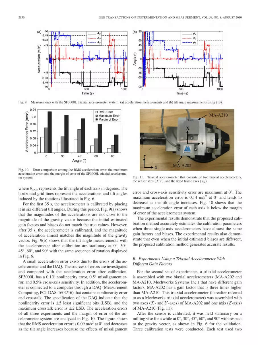
Fig. 9. Measurements with the SF3000L triaxial accelerometer system: (a) acceleration measurements and (b) tilt angle measurements using (13).

Fig. 10. Error comparison among the RMS acceleration error, the maximumacceleration error, and the margin of error of the SF3000L triaxial accelerome-ter system.

where θaxis represents the tilt angle of each axis in degrees. Thehorizontal grid lines represent the accelerations and tilt anglesinduced by the rotations illustrated in Fig. 6.

For the first 35 s, the accelerometer is calibrated by placingit in six different tilt angles. During this period, Fig. 9(a) showsthat the magnitudes of the accelerations are not close to themagnitude of the gravity vector because the initial estimatedgain factors and biases do not match the true values. However,after 35 s, the accelerometer is calibrated, and the magnitudeof acceleration almost matches the magnitude of the gravityvector. Fig. 9(b) shows that the tilt angle measurements withthe accelerometer after calibration are stationary at 0◦, 30◦,45◦, 60◦, and 90◦ with the same sequence of rotation displayedin Fig. 6.

A small acceleration error exists due to the errors of the ac-celerometer and the DAQ. The sources of errors are investigatedand compared with the acceleration error after calibration.SF3000L has a 0.1% nonlinearity error, 0.5◦ misalignment er-ror, and 0.5% cross-axis sensitivity. In addition, the accelerom-eter is connected to a computer through a DAQ (MeasurementComputing, PCI-DAS-1602/16) that contains nonlinearity errorand crosstalk. The specification of the DAQ indicate that thenonlinearity error is ±5 least significant bits (LSB), and themaximum crosstalk error is ±2 LSB. The acceleration errorsof all three experiments and the margin of error of the ac-celerometer system are analyzed in Fig. 10. The figure showsthat the RMS acceleration error is 0.09 m/s2 at 0◦ and decreasesas the tilt angle increases because the effects of misalignment

Fig. 11. Triaxial accelerometer that consists of two biaxial accelerometers,the sensor axes (XY ), and the fixed frame axes (xy).

error and cross-axis sensitivity error are maximum at 0◦. Themaximum acceleration error is 0.14 m/s2 at 0◦ and tends todecrease as the tilt angle increases. Fig. 10 shows that themaximum acceleration error of each axis is below the marginof error of the accelerometer system.

The experimental results demonstrate that the proposed cali-bration method accurately estimates the calibration parameterswhen three single-axis accelerometers have almost the samegain factors and biases. The experimental results also demon-strate that even when the initial estimated biases are different,the proposed calibration method generates accurate results.

B. Experiments Using a Triaxial Accelerometer WithDifferent Gain Factors

For the second set of experiments, a triaxial accelerometeris assembled with two biaxial accelerometers (MA-A202 andMA-A210, Mechworks Systems Inc.) that have different gainfactors. MA-A202 has a gain factor that is three times higherthan MA-A210. This triaxial accelerometer (hereafter referredto as a Mechworks triaxial accelerometer) was assembled withtwo axes (X- and Y -axes) of MA-A202 and one axis (Z-axis)of MA-A210 (Fig. 11).

After the sensor is calibrated, it was held stationary on amilling vise for a while at 0◦, 30◦, 45◦, 60◦, and 90◦ with respectto the gravity vector, as shown in Fig. 6 for the validation.Three calibration tests were conducted. Each test used two


Fig. 12. Calibration of the Mechworks triaxial accelerometer system when the initial estimations of biases are 2.5 V: experiment and simulation results.

Fig. 13. Calibration of the Mechworks triaxial accelerometer system when the initial estimations of biases are 10 V: experiment and simulation results.

Fig. 14. Measurements with the Mechworks triaxial accelerometer: (a) acceleration measurements and (b) tilt angle measurements using (13).

different sets of initial estimated biases: 2.5 and 10 V. Fig. 12illustrates the simulation and experiment results of calibrationwhen the initial estimated biases are close to the true biases ofthe accelerometer system (Baxis,0 = 2.5 V), and Fig. 13 showsthe simulation and experiment results of calibration when theinitial estimated biases (Baxis,0 = 10 V) are far from the truebiases. The experimental results of the Mechworks triaxialaccelerometer have the same trend as the experimental resultsof SF3000L. Fig. 12 shows that the experiment steps agree withthe simulation steps, whereas Fig. 13 does not. In both cases,the results reveal that the experimental calibration parametersconverge to the same values within three iteration steps.

The experiment results of Experiment 3 in Fig. 12 areexpanded in Fig. 14. Fig. 14(a) shows the acceleration mea-surements, and Fig. 14(b) shows the tilt angle measurementsconverted from acceleration measurements using (13). Thefirst 36 s in Fig. 14 reflects the calibration period wherethe initial estimated gain factors of each axis are unity andthe initial estimated biases of each axis are 2.5 V. Since theMechworks accelerometers have the true gain factors less than0.04 V/(m/s2) and the initial estimated biases almost match the

true biases, the first 36 s in Fig. 14(a) shows the accelerationsignal around 0 V with very small fluctuations. However, aftercalibration, the two figures in Fig. 14 show that the accelerationmeasurements match the accelerations induced by the rotationangle sequence illustrated in Fig. 6.

The specifications of Mechworks accelerometers show thatthey have 0.2% nonlinearity error, 1◦ misalignment error, and2% cross-axis sensitivity. The accelerometers are connected toa computer through the same DAQ that was used to connect theColibrys triaxial accelerometer. Fig. 15 shows the RMS accel-eration error, the maximum error, and the margin of error ofMA-A202 and MA-A210 with the DAQ. Fig. 15 shows that theRMS acceleration error is 0.10 m/s2 at 0◦ and tends to decreaseas the tilt angle increases. The maximum acceleration error is0.16 m/s2 at 0◦ and tends to decrease as the tilt angle increases.The maximum error of the system is within the margin oferror of both accelerometer systems. The experimental resultsof the Mechworks triaxial accelerometer demonstrate that theproposed calibration method can accurately estimate the gainfactors and biases of the triaxial accelerometer with differentgain factors.


Fig. 15. Error comparison among the RMS acceleration error, the maximumacceleration error, and the margins of error of the MA-A202 and MA-A210accelerometer system.

V. CONCLUSION

This paper has presented a novel calibration method that de-termines the gain factors and biases of a triaxial accelerometerby orienting the sensor in six different tilt angles. The presentedmethod was developed using the mathematical model of gainfactors and biases. To validate the proposed calibration method,simulations and experiments were performed.

The simulation results showed that the proposed calibrationmethod accurately estimated the gain factors and biases withinthree iteration steps. Since the true gain factors and biases werenot available in experiments, the accelerations measured withan accelerometer after calibration were compared with the trueaccelerations that were calculated from the gravity vector tovalidate the estimated gain factors and biases. The first setof experiments was performed using a triaxial accelerometerconsisting of three single-axis accelerometers that have almostthe same gain factors and biases. The RMS acceleration error ofthe accelerometer after calibration was 0.09 m/s2, and the max-imum error was within the margin of error of the accelerometersystem. The second set of experiments was performed using atriaxial accelerometer that has two different gain factors and al-most the same biases. The RMS acceleration error of the Mech-works triaxial accelerometer after calibration was 0.10 m/s2,and the maximum error was within the margin of error of theaccelerometer system.

From the simulations and experiments, it is concluded thatthe proposed calibration method can be adapted to accuratelyestimate the calibration parameters. The proposed calibrationmethod follows a very simple procedure and has a low com-putational cost. In addition, this method does not require anyprior knowledge of the accelerometer calibration parametersnor the six tilt angles that are needed to implement the iterativeapproach for the proposed calibration.

The proposed method is particularly useful for a low-costtriaxial accelerometer whose initial estimated gain factors andbiases highly vary from switch-on to switch-on because thesimulations and experiments show that the gain factors andbiases can accurately be estimated even when the initial esti-mated gain factors and biases are not close to the true value.In addition, since the proposed method does not require highcomputational power, this method can be used for in-useapplications.

REFERENCES

[1] Y. K. Peng and M. F. Golnaraghi, “A vector-based gyro-free inertialnavigation system by integrating existing accelerometer network in anautomobile,” in Proc. CSME Forum, London, ON, Canada, Jun. 1–4,2004, pp. 421–430.

[2] M. Koifman and I. Y. Bar-Itzhack, “Inertial navigation system aided byaircraft dynamics,” IEEE Trans. Control Syst. Technol., vol. 7, no. 4,pp. 487–493, Jul. 1999.

[3] H. J. Luinge and P. H. Veltink, “Inclination measurement of humanmovement using a 3-D accelerometer with autocalibration,” IEEE Trans.Neural Syst. Rehabil. Eng., vol. 12, no. 1, pp. 112–121, Mar. 2004.

[4] H. J. Luinge, P. H. Veltink, and C. T. M. Baten, “Estimation of orientationwith gyroscopes and accelerometers,” Technol. Health Care, vol. 7, no. 6,pp. 455–459, Jan. 1999.

[5] B. Kemp, A. J. Janssen, and B. van der Kamp, “Body position canbe monitored in 3D using miniature accelerometers and earth-magneticfield sensors,” Electroencephalogr. Clin. Neurophysiol., vol. 109, no. 6,pp. 484–488, Dec. 1998.

[6] E. Foxlin, “Motion tracking requirements and technologies,” in ExtendedDraft Version of Chapter 8 in Handbook of Virtual Environment Technol-ogy, K. Stanney, Ed. Mahwah, NJ: Lawrence Erlbaum Assoc., 2002.

[7] P. H. LaFond, “Modeling for error reduction accelerometers,” in Proc.IEEE PLANS, Mar. 23–27, 1992, pp. 126–132.

[8] M. El-Diasty, A. El-Rabbany, and S. Pagiatakis, “Temperature varia-tion effects on stochastic characteristics for low-cost MEMS-based iner-tial sensor error,” Meas. Sci. Technol., vol. 18, no. 11, pp. 3321–3328,Sep. 2007.

[9] F. Ferraris, U. Grimaldi, and M. Parvis, “Procedure for effortless in-fieldcalibration of three-axis rate gyros and accelerometers,” Sens. Mater.,vol. 7, no. 5, pp. 311–330, 1995.

[10] D. Giansanti, G. Maccioni, and V. Macellari, “Guidelines for calibrationand drift compensation of a wearable device with rate-gyroscopes and ac-celerometers,” in Proc. 29th Annu. Int. Conf. IEEE EMBS, Lyon, France,Aug. 22–26, 2007, pp. 2342–2345.

[11] P. Lang and A. Pinz, “Calibration of hybrid vision/inertial tracking sys-tems,” in Proc. 2nd InerVis Workshop Integr. Vis. Inertial Sens., Apr. 18,2005, pp. 1–6.

[12] A. Umeda, M. Onoe, K. Sakata, T. Fukushia, K. Kanari, andH. T. Kobayashi, “Calibration of three-axis accelerometers using a three-dimensional vibration generator and three laser interferometers,” Sens.Actuators A, Phys., vol. 114, no. 1, pp. 93–101, Aug. 2004.

[13] E. L. Renk, M. Rizzo, W. Collins, F. Lee, and D. S. Bernstein, “Cali-brating a triaxial accelerometer-magnetometer—Using robotic actuationfor sensor reorientation during data collection,” IEEE Control Syst. Mag.,vol. 25, no. 6, pp. 86–95, Dec. 2005.

[14] A. Kim and M. F. Golnaraghi, “Initial calibration of an inertial mea-surement unit using an optical position tracking system,” in Proc. IEEEPLANS, Apr. 26–29, 2004, pp. 96–101.

[15] Z. Dong, G. Zhang, Y. Luo, C. C. Tsang, G. Shi, S. Y. Kwok, W. J. Li,P. H. W. Leong, and M. Y. Wong, “A calibration method for MEMS in-ertial sensors based on optical tracking,” in Proc. IEEE Int. Conf. NEMS,Bangkok, Thailand, Jan. 16–19, 2007, pp. 542–547.

[16] E.-H. Shin and N. El-Sheimy, “A new calibration method for strapdowninertial navigation systems,” Zeitschrift fur Vermessungswesen, vol. 127,no. 1, pp. 41–50, Jan. 2002.

[17] Z. F. Syed, P. Aggarwal, C. Goodall, X. Niu, and N. El-Sheimy, “A newmulti-position calibration method for MEMS inertial navigation systems,”Meas. Sci. Technol., vol. 18, no. 7, pp. 1897–1907, Jul. 2007.

[18] A. Lai, D. A. James, P. Hayes, and E. C. Harvey, “Semi-automatic cal-ibration technique using six inertial frames of reference,” Proc. SPIE,vol. 5274, pp. 531–542, Dec. 10–12, 2003.

[19] J. C. Lötters, J. Schipper, P. H. Veltink, W. Olthius, and P. Bergveld,“Procedure for in-use calibration of triaxial accelerometers in medicalapplications,” Sens. Actuators A, Phys., vol. 68, no. 1–3, pp. 221–228,Jun. 1998.

[20] Z. C. Wu, Z. F. Wang, and Y. Ge, “Gravity based online calibration formonolithic triaxial accelerometers’ gain and offset drift,” in Proc. 4thWorld Congr. Intell. Control Autom., Shanghai, China, Jun. 10–14, 2002,vol. 3, pp. 2171–2175.

[21] A. Spengler, M. Stanton, and M. Rowlands, “Expert systems andquality tools for quality improvement,” in Proc. 7th IEEE Int. Conf.Emerging Technol. Autom., Barcelona, Spain, Oct. 19–21, 1999, vol. 2,pp. 955–962.

[22] Canadian Gravity Standardization Network, Oct. 2, 2008. [Online].Available: http://csrsjava.geod.nrcan.gc.ca/csrsjcpe/GSDreportsEN?user_name=CGIS2658&querytype=CGSN&key=93231965


Seong-hoon Peter Won was born in Busan, Korea,in 1975. He received the B.Sc. and M.A.Sc. degreesin mechanical engineering from the University ofWaterloo, Waterloo, ON, Canada, in 2001 and 2003,respectively.

Since 2006, he has been with the University ofWaterloo, where he was involved in applications inhandheld inertial navigation systems. He researcheson improving the performance of inertial navigationsystems with other position sensors.

Farid Golnaraghi received the B.S. and M.S. de-grees in mechanical engineering from WorcesterPolytechnic Institute, Worcester, MA, both in 1982and the Ph.D. degree in theoretical and applied me-chanics from Cornell University, Ithaca, NY, in 1988.

In 1988, he became a Professor of mechanicalengineering, and later mechanical and mechatron-ics engineering, with the University of Waterloo,Waterloo, ON, Canada. He also became a Tier ICanada Research Chair in mechatronics and smartmaterial systems at Waterloo in 2002. In August

2006, he was the Director of the mechatronics engineering program with SimonFraser University (SFU), Surrey, BC, Canada. He is the holder of a BurnabyMountain endowed Chair. Over the past 20 years in Waterloo and SFU, he hasbeen very active in the supervision of graduate students. His pioneering researchhas resulted in two textbooks, more than a hundred papers, four patents, and twostartup companies.