Mon. Not. R. Astron. Soc. 000, 1–?? () Printed 9 September 2021 (MN LATEX style file v2.2)

Phase space dynamics of triaxial collapse: Jointdensity-velocity evolution

Sharvari Nadkarni-Ghosh1? and Akshat Singhal2†1Department of Physics, I.I.T. Kanpur, Kanpur, U.P. 208016 India2Department of Mathematics and Statistics, I.I.T. Kanpur, Kanpur, U.P. 208016 India

ABSTRACT

We investigate the dynamics of triaxial collapse in terms of eigenvalues of the de-formation tensor, the velocity derivative tensor and the gravity Hessian. Using theBond-Myers model of ellipsoidal collapse, we derive a new set of equations for thenine eigenvalues and examine their dynamics in phase space. The main advantage ofthis form is that it eliminates the complicated elliptic integrals that appear in the axesevolution equations and is more natural way to understand the interplay between theperturbations.

This paper focuses on the density-velocity dynamics. The Zeldovich approximationimplies that the three tensors are proportional; the proportionality constant is set bydemanding ‘no decaying modes’. We extend this condition into the non-linear regimeand find that the eigenvalues of the gravity Hessian and the velocity derivative tensorare related as qd + qv = 1, where the triaxiality parameter q = (λmax−λinter)/(λmax−λmin). This is a new universal relation holding true over all redshifts and a range ofmass scales to within a few percent accuracy. The mean density-velocity divergencerelation at late times is close to linear, indicating that the dynamics is dictated bycollapse along the largest eigendirection. This relation has a scatter, which we show,is intimately connected to the velocity shear. Finally, as an application, we computethe PDFs of the two variables and compare with other forms in the literature.

Key words: cosmology: large-scale structure of Universe

1 INTRODUCTION

Over the last decade or so, observations of the large scale structure in the universe have emerged as a very powerful probe

to constrain cosmological parameters. The two main variables that characterize this structure are the fractional overdensity

δ and the peculiar velocity v. In the linear regime, the two observables are connected as ∇ · v = −fHδ, where H is the

Hubble parameter and f is the growth rate. f is sensitive to the underlying cosmology and surveys such as 6dFGS 1 or

the future EUCLID 2 observe peculiar velocities either directly (e.g., Johnson et al. 2014) or from redshift space distortions

(e.g.,Majerotto et al. 2012) with an aim to place precise constraints on f . It would be ideal if the data followed linear theory,

but observations are sensitive to non-linear effects which can introduce a bias even on linear scales. Therefore, a theoretical

understanding of the non-linear regime is imperative. Numerical simulations and perturbation theories are the two standard

ways of tracking non-linear growth. However, both these methods have drawbacks. N-body codes are slow. Furthermore,

they use a discrete representation of the density field and hence their results are shot-noise limited (for e.g., Joyce, Marcos, &

Baertschiger 2009). Perturbation theories deal with smooth fields but they are not always guaranteed to converge and involved

resummation techniques need to be invoked to get meaningful results (for e.g., Matsubara 2008; Matarrese & Pietroni 2007;

Nadkarni-Ghosh & Chernoff 2011, 2013). Given the plethora of cosmological models, these features can prove to be restrictive.

? E-mail: sharvari@iitk.ac.in† E-mail: akshat.singhal014@gmail.com1 http://www.6dfgs.net/2 http://www.euclid-ec.org/

c© RAS

arX

iv:1

407.

1945

v4 [

astr

o-ph

.CO

] 5

Feb

201

6

2 Sharvari Nadkarni-Ghosh and Akshat Singhal

A third way to model the non-linear regime is to restrict the dynamics to simple geometries. Though based on local

dynamics, such models often give theoretical insight into the underlying physics. The simplest among these is the spherical

collapse model (spherical top-hat). It has been used in a myriad of ways starting from the mid-seventies to the present day. The

critical density for collapse predicted by this model is an important ingredient in the mass function prescription given by Press

& Schechter (1974). It has been widely used to understand the nature of non-linearities in a range of dark energy cosmologies

from ΛCDM to early dark energy and quintessence models (for e.g., see Wintergerst & Pettorino 2010 and references therein).

Kitaura & Heß (2013) have used it in conjunction with Lagrangian perturbation theory to evolve perturbations through the

shell-crossing regime. It has given valuable insights into the joint non-linear density-velocity evolution (Bilicki & Chodorowski

2008; Nadkarni-Ghosh 2013). It has also been proposed as a control case to test the accuracy of N-body codes in the non-linear

regime (Joyce & Sylos Labini 2012). And last but not the least, it has been used to explain the famous NFW profile (Navarro,

Frenk, & White 1996; Lokas 2000) and as well as results of other simulations based on modified gravity (Stabenau & Jain

2006; Martino, Stabenau, & Sheth 2009).

Ellipsoidal or triaxial collapse is the next popular local model. It provides many improvements over the spherical geometry

and has been in consideration for over five decades. Early studies (Lynden-Bell 1964; Lin, Mestel, & Shu 1965) examined the

isolated ellipsoid in a non-expanding background. Cosmological extensions were performed by Icke (1973) and White & Silk

(1979) but under the assumption that the background did not exert external forces on the ellipsoid. Bond & Myers (1996)

included the effect of the background in terms of an external tidal field. Nariai & Fujimoto (1972) and Eisenstein & Loeb

(1995) provided a more complete analytic model that includes rotation as well. Since then, not much has changed in the

theoretical ingredients of the model, however, the number of applications have been on the rise. Effects of non-radial motions

on the growth rate and the resultant modifications to the Press-Schecter mass function were studied by several authors (for

e.g., Monaco 1995; Del Popolo & Gambera 2000; Del Popolo, Ercan, & Xia 2001; Sheth, Mo, & Tormen 2001; Kerscher,

Buchert, & Futamase 2001). Many authors developed alternatives to Press-Schecter that were based on statistics of collapse

times derived from ellipsoidal collapse (Audit, Teyssier, & Alimi 1997; Monaco, Theuns, & Taffoni 2002). Others have obtained

statistical measures of the non-linear density and velocity fields based on ellipsoidal collapse (Fosalba & Gaztanaga 1998a,b;

Scherrer & Gaztaaga 2001; Ohta, Kayo, & Taruya 2003, 2004; Lam & Sheth 2008a,b). Angrick & Bartelmann (2010) used

this model with additional components introduced to treat the virialization epoch. Very recently, Despali, Tormen, & Sheth

(2013) have advocated the use of ellipsoidal halo finders as an improvement over the spherical overdensity method to model

shapes of haloes and this method has been applied to big numerical simulations to get insights into the shape distribution of

dark matter haloes (Bonamigo et al. 2014). Thus, spherical and ellipsoidal collapse models are not only used in isolation to get

insights into the results of simulations, but they are also used in conjunction with numerical techniques to get semi-analytic

estimates or for post-processing numerical data.

One of the reasons why these simple geometries are so popular is that exact analytic solutions are available for homogenous

perturbations evolving in pure matter cosmologies. The collapse in these cases is self-similar and the axes’ lengths (or radius,

in case of sphere) are the primary variables of interest. However, the main observationally relevant variables are the density

and line of sight velocity, or more generally, the gravitational field and the peculiar velocity field. Thus it is more natural and

interesting to directly understand how the these fields evolve in simple geometries. In case of spherical symmetry, the collapse

is radial and only two variables suffice to describe the dynamics: density δ and the velocity divergence Θ. In a recent paper

Nadkarni-Ghosh (2013), hereafter N13, investigated the dynamics of these variables in a two-dimensional density-velocity

divergence phase space 3. A relation between the two variables was obtained by imposing the criterion of ‘no perturbations at

the big bang time’, and it was shown that this traces out a special curve in the 2D phase-space. The flow of perturbations is

such that all perturbations, no matter where they start in phase space, eventually get attracted to this curve. Those that start

along the curve, stay on it to a high degree of accuracy. The attracting nature established that this curve 4 was the desired

non-linear density-velocity relation and it was found that a combination of analytic forms given by Bilicki & Chodorowski

(2008) and Bernardeau (1992) gave a good fit.

In case of a triaxial ellipsoid, the situation is more involved. The full dynamics depends not only on the internal potential,

but also on the external tidal field, which has been treated differently by different authors. The internal gravitational potential

has a quadratic dependence on the length of the principle axes of the ellipsoid (Peebles 1980). In this paper, we follow the

model of Bond & Myers (1996), hereafter BM96, which assumes that the external tidal field is also along the principle axes

of the ellipsoid throughout the evolution. The gravity field can then be described by three variables. These correspond to the

eigenvalues of the tensor of second derivatives of the gravitational potential (henceforth called the ‘gravity Hessian’). In the

absence of rotation, the velocity field also needs three variables. These are the eigenvalues of the tensor of partial derivatives

3 In N13, the velocity perturbation variable was θ = Θ/34 In N13, this curve was termed the ‘Zeldovich curve’ because it is the non-linear extension of the ‘no decaying modes’ criterion, whichis invoked in the linear Zeldovich approximation (Zeldovich 1970); here we call it the SC-DVDR

c© RAS, MNRAS 000, 1–??

Density-velocity evolution from triaxial collapse 3

of the velocity field (also sometimes called the ‘velocity deformation tensor’ 5 and in this work referred to as the ‘velocity

derivative tensor’). These six variables completely describe the gravitational dynamics of the ellipsoid. Since the potential

of the system is intimately connected to its shape, these variables get connected to the eigenvalues of the deformation or

displacement tensor.

In this work, we aim to study the joint evolution of density and velocity through the dynamics of these eigenvalues.

Starting from the BM96 set of equations for triaxial collapse, we obtain a set of coupled one-dimensional differential equations

for the nine eigenvalues. This new set has no dependence on the elliptic functions that appear in the original equations for

the axes lengths and is a well-defined dynamical flow. In §2, we derive these equations and by applying the ‘no perturbations

at the big bang’ condition, we get a relation between the eigenvalues of the gravity Hessian and the velocity derivative tensor.

This traces out a subspace of perturbations, which we call the ‘Zeldovich subspace’ and we find a new universal relation that

describes the perturbations in this subspace. As a by-product, this analysis gives us insight into the relation between the

density and the trace of the deformation tensor. In §3, we examine the dynamics in the 2D δ − Θ space. We investigate the

scatter in the δ − Θ relation and its relation to the velocity shear, thus providing a new insight based on local dynamics.

Finally, as an application, in §4, we numerically compute the marginal one-point probability distribution function (PDF) of

the density and velocity divergence and compare them to some existing forms in the literature. We conclude in §5. Throughout

this paper the terms ‘ellipsoidal’ and ‘triaxial’ are used interchangeably.

2 DYNAMICS OF THE ELLIPSOID

2.1 Notation and equations

Consider a uniform ellipsoidal distribution of cosmological fluid consisting of dark matter and dark energy evolving in a flat,

homogenous and isotropic background. Let ρm,e be the matter density inside the ellipsoid. It differs from the background

matter density ρm; the difference is characterized by the fractional density δ = ρm,e/ρm−1. The dark energy is the same inside

and outside the ellipsoid and is described by a cosmological constant with density ρΛ. Let the origin be at the centre of the

ellipsoid. The ellipsoid can be completely characterized by the evolution of its three principal axes. In this paper we follow the

equations of BM96, which assume that the direction of the axes remains unchanged throughout the evolution. The physical

coordinate of each axis ri can be written as ri = ai(t)q (i = 1, 2, 3), where q is the comoving radius of the corresponding

‘Lagrangian sphere’ (BM96): this is a sphere concentric with the ellipsoid whose mass equals that of the ellipsoid but whose

density is the same as the background. ai are the ‘scale factors’ of each axis and a is the background scale factor. Throughout

this paper we will use the subscript ‘i’ to index the axes and ‘init’ to denote initial conditions. Mass conservation during

evolution implies a3q3ρm = a1a2a3q3ρm,e giving

δ =a3

a1a2a3− 1. (1)

The evolution of ai according to BM96 is 6

d2aidt2

= −4πG

[ρm3− 2

3ρΛ

]ai − 4πG

[ρm

δαi2

+ λext,i

]ai, (2)

where

αi = a1a2a3

∫ ∞0

dτ

(a2i + τ)

∏j=3j=1(a2

j + τ)1/2with

(3∑i=1

αi = 2

)(3)

λext,i =5

4

(αi −

2

3

)non-linear approx. (4)

In eq. (2), the first term in square brackets corresponds to the background potential and the second term to the perturbation

potential. The αis are parameters that describe the internal potential of the ellipsoid and are computed using Carlson’s elliptic

integrals (Carlson 1987, 1989; Press et al. 2002; see appendix B for relations). λext,i(t) models the external tidal field. In this

paper, we will use the non-linear approximation 7. Using standard definitions: ρm = Ωmρc, ρΛ = ΩΛρc and H2 = 8πGρc/3

5 In the past, these have also been referred to as the ‘gravitational shear’ and ‘velocity shear’ tensors respectively. However, we will keepthis terminology only for the traceless part of these tensors.

6 Our notation differs slightly from BM96: αi ≡ bi and λext,i ≡ λ′ext,i in BM96. With this, the two terms δ3

+δb′i2

in BM96 are equal

to δαi2

in our notation.7 A recent paper by Angrick & Bartelmann (2010) experimented with using a hybrid model to compute halo mass functions. They used

the non-linear expression of BM96 at early times and reverted back to the linear expression of BM96 after turn-around. They concludedthat the hybrid model and the non-linear model gave approximately the same results. We prefer to use a single function than a piecewise

one so we stick to the BM96 form

c© RAS, MNRAS 000, 1–??

4 Sharvari Nadkarni-Ghosh and Akshat Singhal

and converting the time variable to a gives

d2aida2

+

1

Ha

d

da(Ha)

· daida

= − 3

2a2

[Ωm(a)

(1

3+δαi2

+ λext,i

)− 2

3ΩX(a)

]ai. (5)

Note that the Ω parameters are functions of a and are related to their values today (a = a0) by

Ωm(a) =Ωm,0H

20a

30

H2a3; ΩΛ(a) =

ΩΛ,0H20

H2. (6)

In this paper we will consider only two cosmologies. The EdS case with Ωm = 1 and ΩΛ = 0 and the ΛCDM case with

Ωm = 0.29 and ΩΛ = 0.71. The evolution of the ellipse is completely determined once six parameters are known: the three

axes lengths ai,init and their velocities ai,init at some initial epoch ainit.

An alternate description of the ellipse can be given by a set of nine dimensionless parameters

λa,i = 1− aia

(7a)

λv,i =1

H

aiai− 1 (7b)

λd,i =δαi2

+ λext,i, (7c)

where i = 1, 2, 3. The eigenvalues λd,i are ordered as λd,1 > λd,2 > λd,3. This implies the ordering λv,1 6 λv,2 6 λv,3 and

λa,1 > λa,2 > λa,3 at all times.

The three λa characterize the shape of the ellipse in terms of the deviation from the background. They correspond to the

eigenvalues of the ‘comoving strain or deformation tensor’ (see Appendix A for definitions) . Because the ellipsoid is always

deformed along its principle axes, the deformation tensor is diagonal at all times. When an axis is collapsing λa → 1, whereas

for an expanding axes, λa → −∞.

The three λv capture the deviation of the velocity of each axes from the background Hubble flow. They correspond to

the eigenvalues of the tensor of (scaled) velocity derivatives. The trace part gives the ‘expansion’

Θ =∇ · vH

= λv,1 + λv,2 + λv,3. (8)

where v = r−Hr. In our definition, a negative λv implies a infall and a positive λv implies expansion. The three eigenvalues

completely describe the curl-free velocity field of this model.

The three λd correspond to the eigenvalues of the gravity Hessian (tensor of second derivatives of the gravitational field).

Equation (7c) comprises of two terms; the first corresponds to the internal potential of the ellipse and the second to the

external tidal field or the traceless gravitational tidal tensor. This definition and the fact that∑i αi = 2, implies

δ = λd,1 + λd,2 + λd,3. (9)

This is also the consistency condition arising from Poisson’s equation.

Not all λs are independent. Equation (7c) defines an implicit relation between the three λd and the three λa (this can be

seen from the definitions of αi and λa,i). In general, this relation is not linear. However, when the perturbations are small,

the Zeldovich approximation implies λa,i = λd,i and λv,i = −λd,i. Equation (9) reduces to

δlin = λa,1 + λa,2 + λa,3. (10)

We emphasize that eq. (10) is not valid in the non-linear regime and we will illustrate the difference in §2.3. Usually it

is standard to characterize the shape of the ellipse in terms of the ‘ellipticity’ e and ‘prolaticity’ p parameters (Bardeen

et al. 1986). These are sometimes defined in terms of λd, but as has been emphasized in the literature (for e.g., Angrick &

Bartelmann 2010), such definitions are valid only in the linear regime. Connecting the shape to λd,i in the non-linear regime

necessarily involves solving for the three axes lengths.

An important assumption in the framework of Bond & Myers is that the principle axes of the deformation tensor and

gravitational shear tensor coincide at all times during the evolution. If this assumption is violated then the ellipsoid can rotate

and additional parameters need to be introduced to describe the dynamics. A more general framework that allows for rotation

has been introduced by Eisenstein & Loeb (1995).

In terms of the λ parameters, the equations eq. (5) and its initial conditions are

d2a

da2+

1

Ha

d

da(Ha)

· dada

= − 3

2a2

[Ωm(a)

1

3+ λd(a)

− 2

3ΩX(a)

]a (11)

ainit = ainit(1− λa,init) (12)

da

da

∣∣∣∣ainit

= ainit(1− λa,init)(1 + λv,init). (13)

We have introduced boldface symbols for quantities that are 3-tuples. The product (1 − λa,init)(1 − λv,init) does not denote

a dot product. It is just the product of the corresponding components for each axes. The boldface a denotes the axes of the

ellipse and a denotes the scale factor of the background.

c© RAS, MNRAS 000, 1–??

Density-velocity evolution from triaxial collapse 5

2.2 Dynamics in phase space

2.2.1 Equations for the eigenvalues

The nine (dimensionless) eigenvalues completely characterize the density, velocity and shape perturbations in this model of

ellipsoidal collapse. In this paper, our focus is on the joint dynamics of density and velocity, hence, in principle, only six

evolution equations are needed: one for each component of λd and λv. These are obtained by their definitions in eqs. (7a),

(7b) and the evolution given by eq. (11). However, it turns out that the equation for λd,i involves complicated functions of aiwhich cannot be inverted easily since in the non-linear regime the relation between λd and the axes is implicit (see Appendix

B). The system simplifies greatly if one adds the parameters λa to the set. Thus, the net system for the nine eigenvalues is

dλa,id ln a

= −λv,i(1− λa,i) (14a)

dλv,id ln a

= −1

2

[3Ωm(a)λd,i − Ωm(a)− 2ΩΛ(a)− 2λv,i + 2λ2

v,i

](14b)

dλd,id ln a

= −(1 + δ)

(δ +

5

2

)−1(λd,i +

5

6

) 3∑j=1

λv,j (14c)

+

(λd,i +

5

6

) 3∑i=1

(1 + λv,i)−(δ +

5

2

)(1 + λv,i)

+∑j 6=i

λd,j − λd,i ·

(1− λa,i)2(1 + λv,i)− (1− λa,j)2(1 + λv,j)

(1− λa,i)2 − (1− λa,j)2,

where

δ =

3∑i=1

λd,i.

In general, the choice of λd,init (or alternatively λa,init) and λv,init is independent. However, when the fluctuations are small, one

generally employs the Zeldovich approximation (Zeldovich 1970), which states that the velocity is proportional to acceleration

and the proportionality constant is set by requiring ‘no growing modes’ (Buchert 1992; Susperregi & Buchert 1997). Physically,

this means that there are no perturbations at the big bang epoch. At early epochs, when Ωm ≈ 1, this gives the relation

λa = λd and λv = −λd. More generally, λv = −f(Ωm)λd, where f(Ωm) = Ω0.55m is the linear growth rate (Linder 2005; we

have ignored the weak Λ dependence). The linear density-velocity divergence is

Θlin = −f(Ωm)δlin. (15)

2.2.2 The Zeldovich subspace

There are two approaches when we consider extension to the non-linear regime. One way is to initialize the system in the linear

regime, evolve eqs. (14a) to (14c) into the non-linear regime and analyze the resulting λd − λv at any later time. However,

there is no guarantee that the resulting 6-tuples are universal; i.e. they may change with initial conditions. An alternate

approach is to extend the essence of the Zeldovich approximation into the non-linear regime. That is, given three λds one

has to choose the three λvs (or vice versa) which satisfy the condition ‘no perturbations at the big bang’. This condition sets

a special relation between the λd and the λv and we denote the resulting 6-tuples as (λd,λZelv ). This set defines a subspace

in the 6D phase space which we call the ‘Zeldovich subspace’. Since there are only three independent parameters, this space

is 3-dimensional. The superscript appears only on λv to denote λv is a function of λd (our convention). Computationally,

λZelv is obtained as follows. Given the λd, first compute the λa from the implicit relation eq. (7c). This acts as a known

initial condition for eq. (11). Then backward integrate eq. (11) with λv as a unknown initial value which is solved for three

simultaneous conditions a(a = 0) = 0. It does not suffice to solve for only one or two of the axes. δ = 0 at a = 0 only when

all three axes are zero simultaneously. The value for ainit is taken to be the epoch for which the λd − λv relation is desired.

The two approaches are complementary and it is not obvious that they will give identical results. A different set of

initial conditions (for example, those that violated the Zeldovich approximation) could, in principle, generate future (λd,λv)

values that need not satisfy the non-linear Zeldovich criterion (i.e., no perturbations at the big bang). However, we find that

this is not the case. All perturbations, irrespective of whether they initially satisfy the Zeldovich approximation, satisfy the

same λd − λv relation at late times, suggesting a universal behaviour. This universality is tested as follows. This test is for

universality is performed as follows. We track the trajectory of a set of initial points (λd,init,λv,init) using the eigenvalue

equations and examine how much each trajectory deviates from the Zeldovich subspace at late times. The initial conditions

at a = 0.001 are drawn from the distribution given below (Doroshkevich (1970); see Rossi 2012 and Angrick 2013 for recent

c© RAS, MNRAS 000, 1–??

6 Sharvari Nadkarni-Ghosh and Akshat Singhal

æ æ æ æ æ æ æ

æ

æ

à

à

à

à

à

à

à

à

à

à à à à

à

à

à

0.001 0.01 0.1 1

0.1

1

10

100

a

%<

D>

EdS

æ æ æ æ æ ææ

ææ

à

à

à

à

à

à

à

à

à

à à àà

à

à à

ì

ì

ì

ì

ì

ì

ìì

0.001 0.01 0.1 1

0.1

1

10

100

a

%<

D>

LCDM

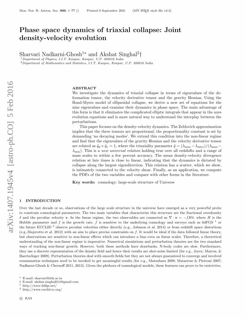
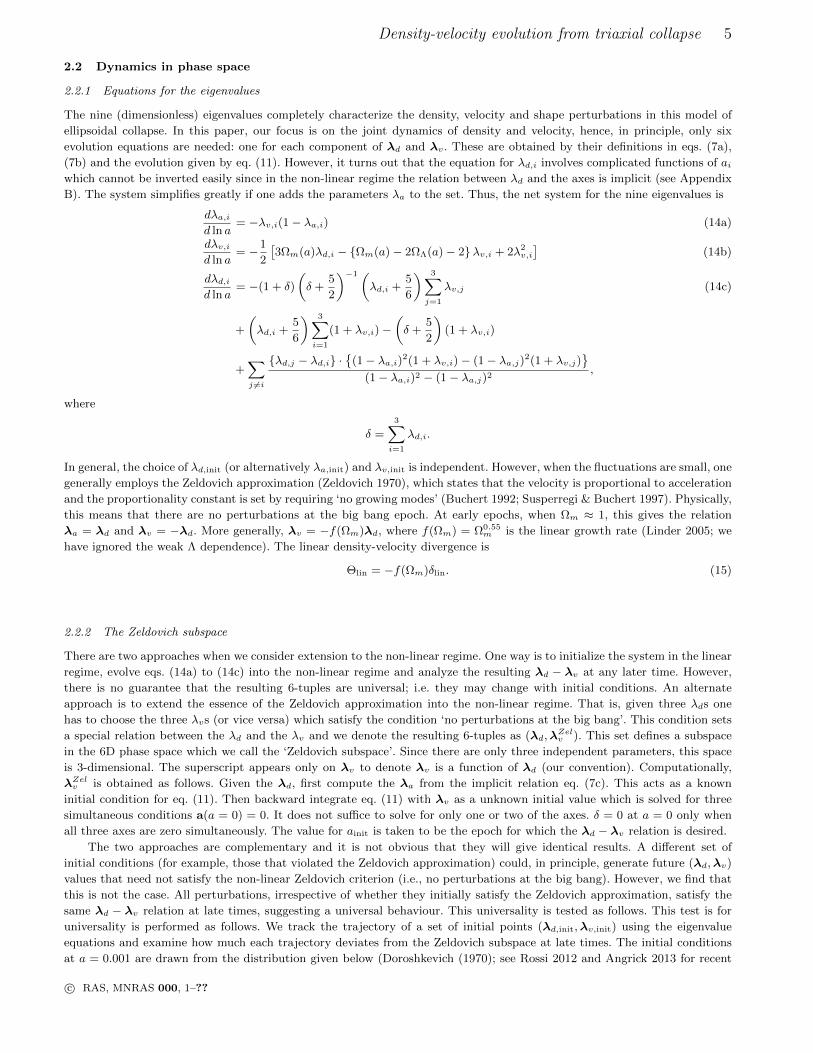
Figure 1. The attracting nature of the Zeldovich subspace: the solid (dashed) lines correspond to λv,init = −λd,init (λv,init = −2λd,init).

The latter set has a 100% deviation at the initial time a = 0.001. For the ΛCDM case an additional non-collinear set λv,init =(−2,−3,−4) · λd,init, where · implies component wise product) was considered (denoted by the dot-dashed lines). This set has a initial

deviation of 216%. The deviation decreases as a power law in a scaling as ∼ a−2.6 for both EdS and ΛCDM cosmologies.

extensions)

p(λd,1, λd,2, λd,3) =153

8π√

5σ6G

exp

(−3I2

1

σ2G

+15I22σ2

G

)· (λd,1 − λd,2)(λd,2 − λd,3)(λd,1 − λd,3), (16)

where σG ≡ σG(Rf ), the r.m.s. density fluctuation at the scale Rf , I1 = λd,1+λd,2+λd,3 and I2 = λd,1λd,2+λd,2λd,3+λd,1λd,3.

This PDF is gives the value at a = 1; the value at a = 0.001 is obtained by multiplying by the appropriate linear growth

factor D+(a) = 5Ωm,0/2∫ a

0[a′H(a′)/H0]−3da (Dodelson 2003). Each point is evolved according to eqs. (14a) to (14c). At a

future epoch, a point on this trajectory is a 6-tuple denoted by λevold ,λvevol. For this λevold , we compute the corresponding

λZelv as described above. This gives the corresponding point in the Zeldovich subspace denoted as λevold ,λZelv . The distance

between λevold ,λvevol and λevold ,λZelv is a measure of how close the trajectory gets to the Zeldovich subspace. We define

the relative deviation at any epoch as

∆(a) =||λevolv (a)− λZelv (a)||

||λZelv (a)||, (17)

where, ||x− y|| denotes the norm√∑

i(xi − yi)2, i = 1, 2, 3.

Figure 1 shows the average (over 50 points) relative deviation as a function of a for the EdS (left panel) and ΛCDM

models (right). For the EdS case, two sets of initial conditions were considered. The first set (solid line) was initialized at

a = 0.001 using the linear relation: λv,init = −λd,init and the second (dashed line) with λv,init = −2λd,init. In the first set, the

error between the linear limit and the exact values that lie in the Zeldovich subspace was found to be 0.1%. This value was

set as a measure of the tolerance i.e. at any other epoch, the error was chosen to be the maximum of the mean deviation and

the tolerance. It was found that at most future epochs, the error stays within 0.1% but rises to about 1% near a = 1. The

second set of initial conditions corresponds to 100% deviation at a = 0.001. The relative deviation drops down exponentially

from ∼ 100% at a = 0.001 to the sub percent level at a = 0.1. This implies that even trajectories that start far off from the

Zeldovich subspace eventually find their way onto it. For this set of initial conditions too, the error rises slightly near a ∼ 1.

Similar behaviour is observed for the ΛCDM case. In this case, an additional third non-collinear set (dot-dashed line) of initial

conditions was considered λv,init = −2,−3,−4 · λd,init i.e., the x, y and z components are twice, thrice and four times the

linear value. The initial deviation in this case is 216%, but again it drops down exponentially. The latter two sets of initial

conditions clearly illustrate the attracting nature of the Zeldovich subspace, but the reason for this late time rise is not yet

fully clear.

Some insight may be gained by looking at it from the point of view of Lagrangian Perturbation Theory (LPT). The

Zeldovich approximation is the first order term in the LPT series (Buchert 1992) and it implies that there are no decaying

modes at this order. In this construction, there may be decaying modes in the higher order solution. Requiring that there be

‘no perturbations at the big bang’ is equivalent to demanding that there be ‘no growing modes’ at every order in the LPT

series (see Ehlers & Buchert 1997; Nadkarni-Ghosh & Chernoff 2013 for the general LPT series construction). Thus, the two

solutions, one obtained by imposing ‘no growing modes’ initially and then evolving and the other obtained by imposing ‘no

growing modes at every order’ are different and the differences could potentially grow at late times. Whether this explains

the observed behaviour quantitatively is yet to be understood and is beyond the scope of this paper. Here, it suffices to note

that compared to the initial deviation from the Zeldovich subspace (∼ 100 %) the final deviation is two orders of magnitude

smaller.

In recent work (N13), this technique was applied to spherical perturbations. It was shown that the non-linear density-

c© RAS, MNRAS 000, 1–??

Density-velocity evolution from triaxial collapse 7

0.0 0.2 0.4 0.6 0.8 1.00.0

0.2

0.4

0.6

0.8

1.0

qd

q v

ΣG= 0.5

ΣG= 0.8

ΣG= 1.0

0 0.2 0.4 0.6 0.8 10.0001

0.001

0.01

a

Max

Èq v+

q d-

1È

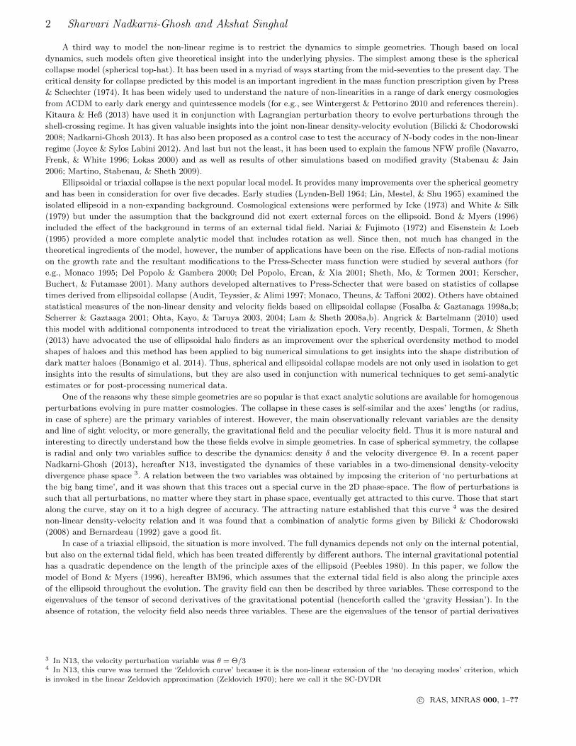
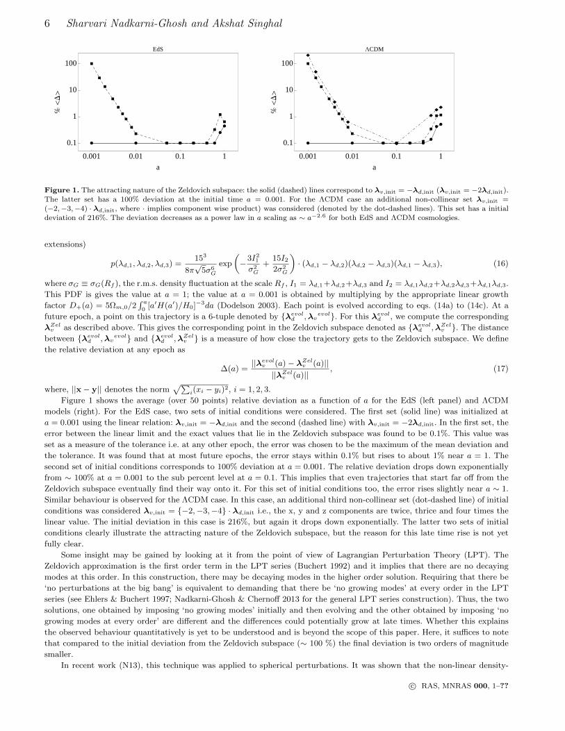
Figure 2. A universal velocity-gravity relation: The left panel plots the triaxiality parameter paris (qd, qv) for a single realization (σG = 1

at a = 1) in the ΛCDM cosmology. The pairs lie on a straight line defined by qv + qd = 1. The error in the relation is plotted in the rightpanel. The error increases with epoch, but stays within 2% for the range of σGs considered here.

velocity relation traced out a universal curve which satisfied the form

Θsph =

32Ωγ1m

[1− (1 + δsph)

23

Ωγ2m

]−1 6 δsph < 1

Ωγ1+γ2m

[(1 + δsph)

16 − (1 + δsph)

12

]δsph > 1

(18)

with γ1 = 0.56 and γ2 = −0.01 for a ΛCDM cosmology. This density-velocity divergence formula based on spherical collapse

is a combination of the forms of Bernardeau (1992) and Bilicki & Chodorowski (2008) and henceforth will be referred to as

the ‘SC-DVDR’. This curve is time-invariant for an EdS cosmology, but changes for the ΛCDM case due to the variation of

Ωm throughout evolution.

2.2.3 A universal non-linear λd − λv relation

We find that it is possible to characterize the universality of the λd−λv relation in terms of triaxiality parameters (s and q).

These are generally defined in the study of axis ratios (Schneider, Frenk, & Cole 2012; Nadkarni-Ghosh & Singhal 2015), in

terms of the major and minor axes or alternatively in terms of the eigenvalues of the deformation tensor. Here, we generalize

the definitions to eigenvalues of any 3-dimensional tensor.

s =1− λmax

1− λmin(19)

q =1− λinter

1− λmin(20)

q =q − s1− s =

λmax − λinter

λmax − λmin, (21)

where, λmax/min/inter denote the maximum, minimum and intermediate eigenvalues. By construction, q is smaller than unity.

We find that, to a very good approximation, the λd − λv relation is given by

qv + qd = 1, (22)

where the subscripts d and v refer to the gravity Hessian and the velocity derivative tensor respectively. It is easy to see

that this relation is satisfied in the linear regime because λd,max = −λv,min and vice versa. Figure 2 illustrates this relation

(left panel) and its accuracy (right panel). The left panel plots the qd, qv pairs for a single realization (∼ 10,000 points)

corresponding to σG = 1 at a = 1 for the ΛCDM cosmology. As a measure of the accuracy of the relation, we compute

Max|qv + qd − 1|, where the maximum is taken over 50,000 points (five realizations). The right panel plots this error as a

function of a for three different values of σG. The accuracy of the relation decreases with epoch, but stays within 2%. This

relation is a ratio of differences, and since the primary dependence of the velocity-gravity relation is through the linear growth

factor, we expect this to be valid for other cosmologies as well (i.e. for other values of Ωm and ΩΛ). Thus, it is universal, not

only with respect to redshift and the mass scale (σG), but also with respect to certain standard dark energy models.

We found the above relation somewhat serendipitously while studying the behaviour of axis ratios Nadkarni-Ghosh &

Singhal (2015). The PDF of the q parameter for the deformation tensor turns out to be an invariant of the dynamics (to

percent level accuracy), and it was natural to investigate the behaviour of the corresponding q parameter for the gravity

Hessian and the velocity derivative tensor. The pattern of the PDFs for qv and qd suggested that qd + qv was a constant,

equal to one. The Zeldovich subspace is three dimensional. To completely describe this subspace analytically, one requires two

c© RAS, MNRAS 000, 1–??

8 Sharvari Nadkarni-Ghosh and Akshat Singhal

a=1, z=0

-1 0 1 2 3-3

-2

-1

0

1

Λd1

Λv 1

EdS

a=1, z=0

-1 0 1 2 3-3

-2

-1

0

1

Λd2

Λv 2

EdS

a=1, z=0

-1 0 1 2 3-3

-2

-1

0

1

Λd3

Λv 3

EdS

a=1, z=0

-1 0 1 2 3-3

-2

-1

0

1

Λd1

Λv 1

LCDM

a=1, z=0

-1 0 1 2 3-3

-2

-1

0

1

Λd2Λ

v 2

LCDM

a=1, z=0

-1 0 1 2 3-3

-2

-1

0

1

Λd3

Λv 3

LCDM

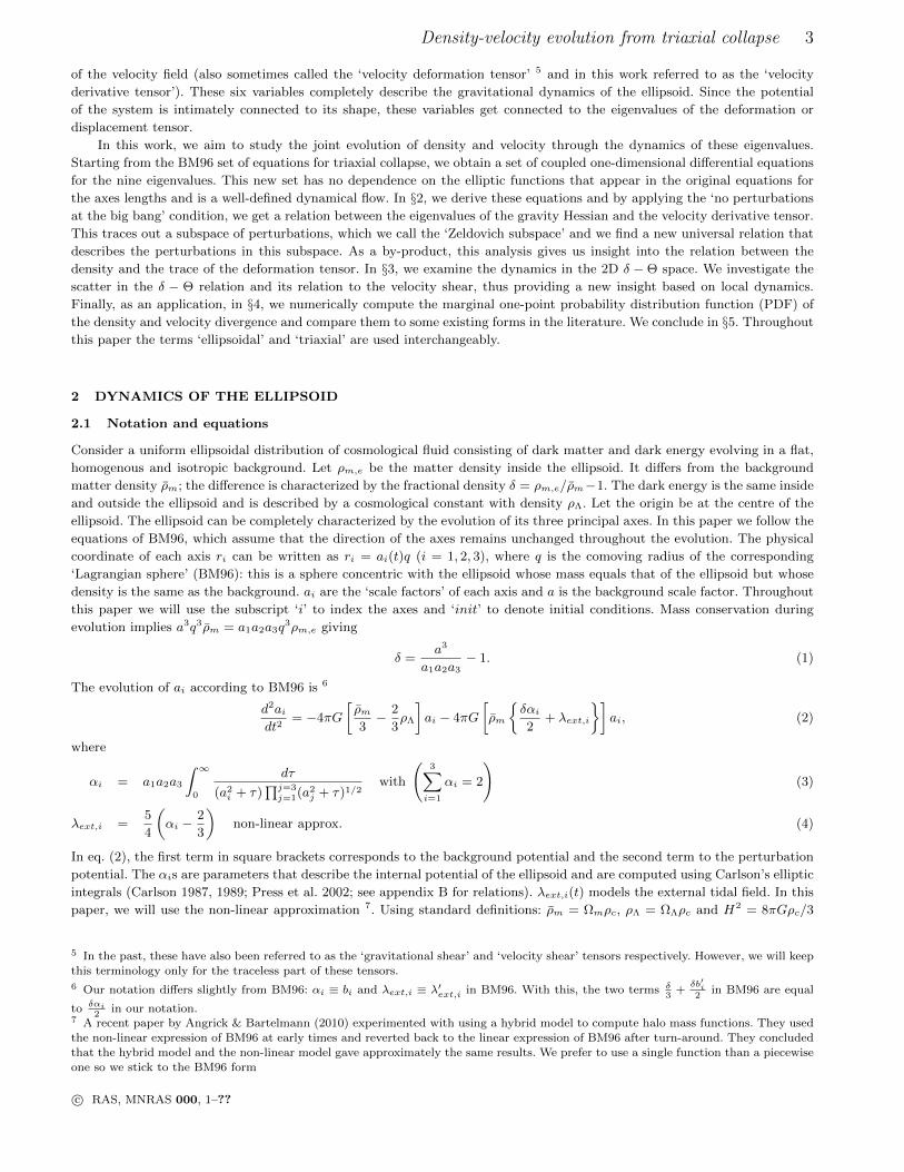
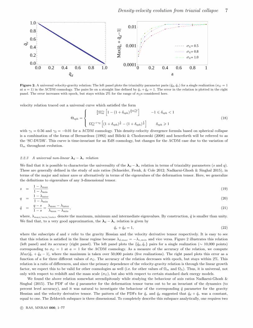
Figure 3. Snapshot at a = 1 of the 2D λd − λv slices of the subspace. The solid line is the SC-DVDR given by eq. (18) and the dashed

line is the linear relation λv = −λd. The first panel corresponds to the largest eigenvalues. The ‘mean’ relation between them is very

close to the linear relation. This is also responsible for the mean δ − Θ relation being close to linear, although to a lesser extent (seefigure 5).

additional independent equations connecting the λds and λvs. More detailed investigations of the phase space equations will

be necessary to construct appropriate invariants and are beyond the scope of this paper.

2.2.4 2D λd − λv subspaces

The entire Zeldovich subspace of the 6D phase space cannot be visualized directly. Nevertheless, it helps to visualize 2D

subspaces defined by the parameters (λd,i, λv,i). Figure 3 shows three such projections at a = 1. In each plot, the dotted line

shows the linear relation λv,i = −f(Ωm)λd,i. The solid curved line is the SC-DVDR given by eq. (18); in this case, λd =δsph

3

and λv =Θsph

3, where δsph and Θsph are given by eq. (18). The main interesting point observed here is that the ‘mean’ relation

between the largest eigenvalue λd,1 and the corresponding λv,1 is close to the linear one. It is clear that in the non-linear regime,

each axes has a different relation between λd and λv i.e., the ‘vectors’ λd and λv are no longer proportional. This means that

although in the triaxial model, the gravitational shear tensor and velocity derivative tensor always have the same principle

axes, their eigenvalues are not simple multiples of each other. This is related to the fact that the gravitational acceleration

and peculiar velocity are not parallel to each other in the non-linear regime, which has been discussed earlier in the context

of Lagrangian perturbation theory (for e.g., Bagla & Padmanabhan 1996; Susperregi & Buchert 1997; Nadkarni-Ghosh &

Chernoff 2013). We also note the distinction between the breakdown of parallelism and breakdown of proportionality; for e.g.

for the sphere with a radially dependent overdensity, the acceleration and velocity in the non-linear regime are always parallel

at any point (both are radial), but yet as fields they are not proportional.

2.3 δ vs. trace of the deformation tensor

Using the phase space evolution one can also investigate the relation between the exact non-linear density δ =∑i λd,i and its

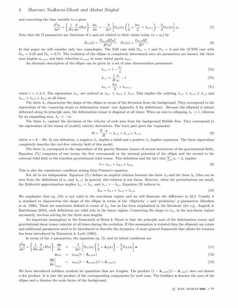
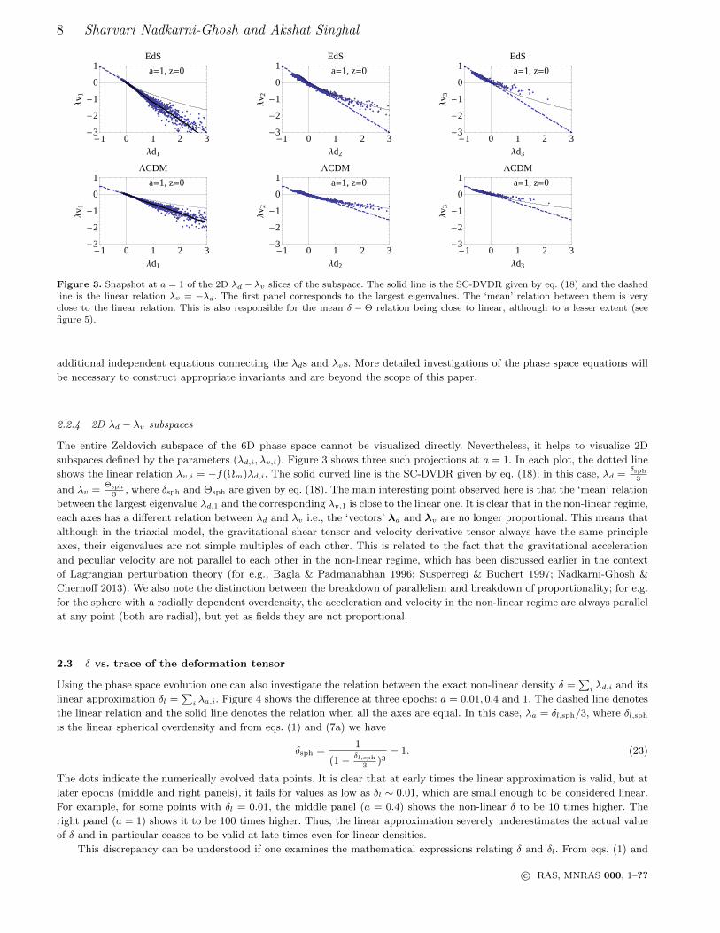
linear approximation δl =∑i λa,i. Figure 4 shows the difference at three epochs: a = 0.01, 0.4 and 1. The dashed line denotes

the linear relation and the solid line denotes the relation when all the axes are equal. In this case, λa = δl,sph/3, where δl,sph

is the linear spherical overdensity and from eqs. (1) and (7a) we have

δsph =1

(1− δl,sph3

)3− 1. (23)

The dots indicate the numerically evolved data points. It is clear that at early times the linear approximation is valid, but at

later epochs (middle and right panels), it fails for values as low as δl ∼ 0.01, which are small enough to be considered linear.

For example, for some points with δl = 0.01, the middle panel (a = 0.4) shows the non-linear δ to be 10 times higher. The

right panel (a = 1) shows it to be 100 times higher. Thus, the linear approximation severely underestimates the actual value

of δ and in particular ceases to be valid at late times even for linear densities.

This discrepancy can be understood if one examines the mathematical expressions relating δ and δl. From eqs. (1) and

c© RAS, MNRAS 000, 1–??

Density-velocity evolution from triaxial collapse 9

a=0.01; z=99

0.001 0.01 0.1 1 10

0.01

0.1

1

10

100

∆l HS Λa,iL

∆HS

Λd,

iLa=0.4; z=1.5

0.001 0.01 0.1 1 10

0.01

0.1

1

10

100

∆l HS Λa,iL

∆HS

Λd,

iL

a=1; z=0

0.001 0.01 0.1 1 10

0.01

0.1

1

10

100

∆l HS Λa,iL

∆HS

Λd,

iL

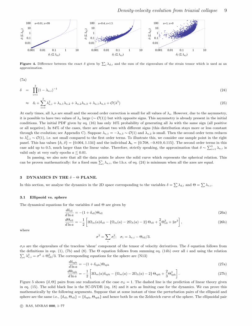
Figure 4. Difference between the exact δ given by∑i λd,i and the sum of the eigenvalues of the strain tensor which is used as an

approximation.

(7a)

δ =

3∏i=1

(1− λa,i)−1 (24)

≈ δl +

3∑i=1

λ2a,i + λa,1λa,2 + λa,2λa,3 + λa,1λa,3 +O(λ3) (25)

At early times, all λas are small and the second order correction is small for all values of λa. However, due to the asymmetry,

it is possible to have two values of λa large (∼ O(1)) but with opposite signs. This asymmetry is already present in the initial

conditions. The initial PDF given by eq. (16) has only 16% probability of generating all λs with the same sign (all positive

or all negative). In 84% of the cases, there are atleast two with different signs (this distribution stays more or less constant

through the evolution; see Appendix C). Suppose λa,1 = −λa,3 ∼ O(1) and λa,2 is small. Then the second order term reduces

to λ2a,1 ∼ O(1), i.e. not small compared to the first order terms. To illustrate this, we consider one sample point in the right

panel. This has values δl, δ = 0.004, 1.134 and the individual λa = 0.708,−0.819, 0.115. The second order terms in this

case add up to 0.5, much larger than the linear value. Therefore, strictly speaking, the approximation that δ ∼∑3i=1 λa,i is

valid only at very early epochs a . 0.01.

In passing, we also note that all the data points lie above the solid curve which represents the spherical relation. This

can be proven mathematically: for a fixed sum∑i λa,i, the l.h.s. of eq. (24) is minimum when all the axes are equal.

3 DYNAMICS IN THE δ −Θ PLANE.

In this section, we analyse the dynamics in the 2D space corresponding to the variables δ =∑λd,i and Θ =

∑λv,i.

3.1 Ellipsoid vs. sphere

The dynamical equations for the variables δ and Θ are given by

dδell

d ln a= −(1 + δell)Θell (26a)

dΘell

d ln a= −1

2

[3Ωm(a)δell − Ωm(a)− 2ΩΛ(a)− 2Θell +

2

3Θ2

ell + 2σ2

], (26b)

where

σ2 =∑i

σ2i ; σi = λv,i −Θell/3.

σis are the eigenvalues of the traceless ‘shear’ component of the tensor of velocity derivatives. The δ equation follows from

the definitions in eqs. (1), (7b) and (8). The Θ equation follows from summing eq. (14b) over all i and using the relation∑i λ

2v,i = σ2 + Θ2

ell/3. The corresponding equations for the sphere are (N13)

dδsph

d ln a= −(1 + δsph)Θsph (27a)

dΘsph

d ln a= −1

2

[3Ωm(a)δsph − Ωm(a)− 2ΩΛ(a)− 2Θsph +

2

3Θ2

sph

]. (27b)

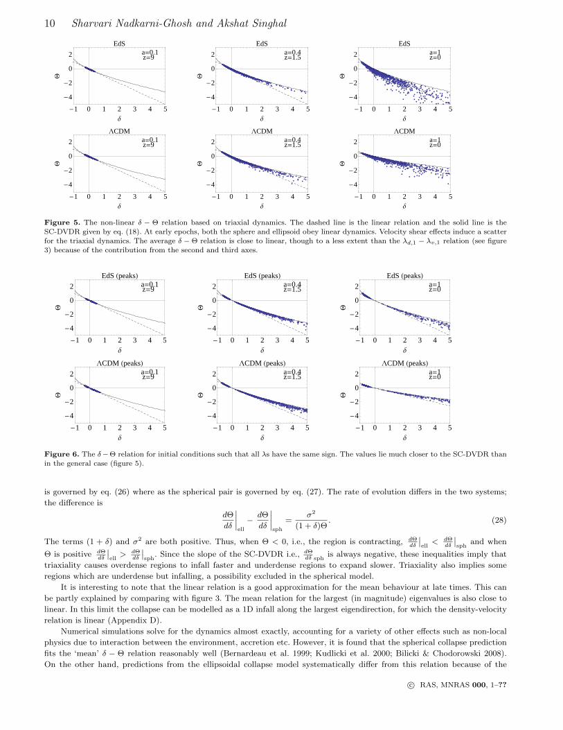
Figure 5 shows δ,Θ pairs from one realization of the case σG = 1. The dashed line is the prediction of linear theory given

in eq. (15). The solid black line is the SC-DVDR (eq. 18) and it acts as limiting case for the dynamics. We can prove this

mathematically by the following arguments. Suppose that at some instant of time the perturbation pairs of the ellipsoid and

sphere are the same i.e., δell,Θell = δsph,Θsph and hence both lie on the Zeldovich curve of the sphere. The ellipsoidal pair

c© RAS, MNRAS 000, 1–??

10 Sharvari Nadkarni-Ghosh and Akshat Singhal

a=0.1z=9

-1 0 1 2 3 4 5

-4

-2

0

2

∆

Q

EdSa=0.4z=1.5

-1 0 1 2 3 4 5

-4

-2

0

2

∆

Q

EdSa=1z=0

-1 0 1 2 3 4 5

-4

-2

0

2

∆

Q

EdS

a=0.1z=9

-1 0 1 2 3 4 5

-4

-2

0

2

∆

Q

LCDMa=0.4z=1.5

-1 0 1 2 3 4 5

-4

-2

0

2

∆Q

LCDMa=1z=0

-1 0 1 2 3 4 5

-4

-2

0

2

∆

Q

LCDM

Figure 5. The non-linear δ − Θ relation based on triaxial dynamics. The dashed line is the linear relation and the solid line is the

SC-DVDR given by eq. (18). At early epochs, both the sphere and ellipsoid obey linear dynamics. Velocity shear effects induce a scatter

for the triaxial dynamics. The average δ −Θ relation is close to linear, though to a less extent than the λd,1 − λv,1 relation (see figure3) because of the contribution from the second and third axes.

a=0.1z=9

-1 0 1 2 3 4 5

-4

-2

0

2

∆

Q

EdS HpeaksLa=0.4z=1.5

-1 0 1 2 3 4 5

-4

-2

0

2

∆

Q

EdS HpeaksLa=1z=0

-1 0 1 2 3 4 5

-4

-2

0

2

∆Q

EdS HpeaksL

a=0.1z=9

-1 0 1 2 3 4 5

-4

-2

0

2

∆

Q

LCDM HpeaksLa=0.4z=1.5

-1 0 1 2 3 4 5

-4

-2

0

2

∆

Q

LCDM HpeaksLa=1z=0

-1 0 1 2 3 4 5

-4

-2

0

2

∆

Q

LCDM HpeaksL

Figure 6. The δ−Θ relation for initial conditions such that all λs have the same sign. The values lie much closer to the SC-DVDR thanin the general case (figure 5).

is governed by eq. (26) where as the spherical pair is governed by eq. (27). The rate of evolution differs in the two systems;

the difference is

dΘ

dδ

∣∣∣∣ell

− dΘ

dδ

∣∣∣∣sph

=σ2

(1 + δ)Θ. (28)

The terms (1 + δ) and σ2 are both positive. Thus, when Θ < 0, i.e., the region is contracting, dΘdδ

∣∣ell< dΘ

dδ

∣∣sph

and when

Θ is positive dΘdδ

∣∣ell> dΘ

dδ

∣∣sph

. Since the slope of the SC-DVDR i.e., dΘdδ sph

is always negative, these inequalities imply that

triaxiality causes overdense regions to infall faster and underdense regions to expand slower. Triaxiality also implies some

regions which are underdense but infalling, a possibility excluded in the spherical model.

It is interesting to note that the linear relation is a good approximation for the mean behaviour at late times. This can

be partly explained by comparing with figure 3. The mean relation for the largest (in magnitude) eigenvalues is also close to

linear. In this limit the collapse can be modelled as a 1D infall along the largest eigendirection, for which the density-velocity

relation is linear (Appendix D).

Numerical simulations solve for the dynamics almost exactly, accounting for a variety of other effects such as non-local

physics due to interaction between the environment, accretion etc. However, it is found that the spherical collapse prediction

fits the ‘mean’ δ − Θ relation reasonably well (Bernardeau et al. 1999; Kudlicki et al. 2000; Bilicki & Chodorowski 2008).

On the other hand, predictions from the ellipsoidal collapse model systematically differ from this relation because of the

c© RAS, MNRAS 000, 1–??

Density-velocity evolution from triaxial collapse 11

0.5 1 2 5 100.01

0.1

1

10

1+ ∆

shea

rsc

alar

0.5 1 2 5 100.01

0.1

1

10

1+ ∆

scat

ter

0.5 1 2 5 100.01

0.1

1

10

1+ ∆

shea

rsc

alar

sca

tter

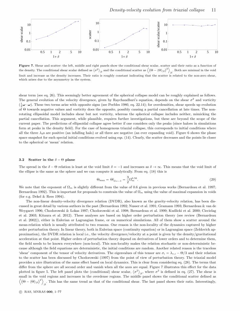
Figure 7. Shear and scatter: the left, middle and right panels show the conditional shear scalar, scatter and their ratio as a function of

the density. The conditional shear scalar defined as⟨σ2⟩|δ and the conditional scatter as

⟨(Θ− 〈Θ〉|δ

)2⟩|δ

. Both are minimal in the void

limit and increase as the density increases. Their ratio is roughly constant indicating that the scatter is related to the non-zero shear,

which arises due to the asymmetry in the system.

shear term (see eq. 26). This seemingly better agreement of the spherical collapse model can be roughly explained as follows.

The general evolution of the velocity divergence, given by Raychaudhuri’s equation, depends on the shear σ2 and vorticity

( 12ω ·ω). These two terms arise with opposite signs (see Peebles 1980, eq. 22.14); for overdensities, shear speeds up evolution

of Θ towards negative values and vorticity does the opposite, possibly causing a partial cancellation at late times. The non-

rotating ellipsoidal model includes shear but not vorticity, whereas the spherical collapse includes neither, mimicking the

partial cancellation. This argument, while plausible, requires further investigations, but these are beyond the scope of the

current paper. The predictions of ellipsoidal collapse agree better if one considers only the peaks (since haloes in simulations

form at peaks in the density field). For the case of homogenous triaxial collapse, this corresponds to initial conditions where

all the three λds are positive (an infalling halo) or all three are negative (an ever expanding void). Figure 6 shows the phase

space snapshot for such special initial conditions evolved using eqs. (14). Clearly, the scatter decreases and the points lie closer

to the spherical or ‘mean’ relation.

3.2 Scatter in the δ −Θ plane

The spread in the δ −Θ relation is least at the void limit δ = −1 and increases as δ →∞. This means that the void limit of

the ellipse is the same as the sphere and we can compute it analytically. From eq. (18) this is

Θmax = Θ|δ=−1 =3

2Ω0.56m . (29)

We note that the exponent of Ωm is slightly different from the value of 0.6 given in previous works (Bernardeau et al. 1997;

Bernardeau 1992). This is important for proposals to constrain the value of Ωm using the value of maximal expansion in voids

(for e.g. Dekel & Rees 1994).

The non-linear density-velocity divergence relation (DVDR), also known as the gravity-velocity relation, has been dis-

cussed in great detail by various authors in the past (Bernardeau 1992; Nusser et al. 1991; Gramann 1993; Bernardeau & van de

Weygaert 1996; Chodorowski & Lokas 1997; Chodorowski et al. 1998; Bernardeau et al. 1999; Kudlicki et al. 2000; Ciecielag

et al. 2003; Kitaura et al. 2012). These analyses are based on higher order perturbation theory (see review (Bernardeau

et al. 2002)), either in Eulerian or Lagrangian frame, or on numerical simulations. All of them show a scatter around the

mean-relation which is usually attributed to two reasons. One reason is the non-locality of the dynamics captured by higher

order perturbation theory. In linear theory, both in Eulerian space (continuity equation) or in Lagrangian space (Zeldovich ap-

proximation), the DVDR relation is local i.e., the velocity divergence/velocity at a point is given by the density/gravitational

acceleration at that point. Higher orders of perturbation theory depend on derivatives of lower orders and to determine them,

the field needs to be known everywhere (non-local). This non-locality makes the relation stochastic or non-deterministic be-

cause although the field equations are deterministic, the initial conditions are random. Another related reason is the traceless

‘shear’ component of the tensor of velocity derivatives. The eigenvalues of this tensor are σi = λv,i − Θ/3 and their relation

to the scatter has been discussed by Chodorowski (1997) from the point of view of perturbation theory. The triaxial model

provides a nice illustration of the same effect based on local dynamics. This is clear from considering eq. (28). The terms that

differ from the sphere are all second order and vanish when all the axes are equal. Figure 7 illustrates this effect for the data

plotted in figure 5. The left panel plots the (conditional) shear scalar,⟨σ2⟩|δ, where σ2 is defined in eq. (27). The shear is

small in the void regions and increases in the overdense regions. The middle panel shows the conditional scatter defined as⟨(Θ− 〈Θ〉|δ

)2⟩|δ

. This has the same trend as that of the conditional shear. The last panel shows their ratio. Interestingly,

c© RAS, MNRAS 000, 1–??

12 Sharvari Nadkarni-Ghosh and Akshat Singhal

this ratio is roughly constant over two decades in density 8. Thus, the scatter can be attributed to the asymmetry in the

system. Indeed, the non-linear DVDR based on the spherical collapse model, which is both local and symmetric, and shows

no scatter.

4 MARGINAL PROBABILITIES p(Θ) AND p(δ).

As an application of this method, we compute the marginal probabilities p(Θ) and p(δ) and qualitatively discuss the joint

PDF p(δ,Θ).

4.1 Numerical runs

The numerical runs were performed by evolving a set of 104 initial conditions using the equations of phase space dynamics

given in eq. (14). At the desired final time the δ and Θ are computed according to definitions given in eqs. (9) and (8). Each

set was drawn from the distribution given by eq. (16). Three scales were considered: σG = 0.5, 1 and 2. The initial σG is

related to the scale of the perturbation: the exact dependence depends on the shape and amplitude of the power-spectrum.

For the BBKS power spectrum with ns = 1 and σ8 = 0.9, σG = 0.5, 1, 2 corresponds to length scales of Rf = 16.4,7 and 3.65

h−1Mpc respectively. Two cosmologies were considered: EdS (Ωm = 1,ΩΛ = 0) and ΛCDM (Ωm = 0.29,ΩΛ = 0.71). The

realization at a = 1 was the same for the two cosmologies, but the values at the initial epoch a = 0.001 were set by multiplying

by the correct growth rate factor. By a = 1 roughly one-tenth of the points had undergone collapse. For each σG value, five

realizations were evolved; the PDF is the average over five and the error bars correspond to the standard deviation.

4.2 Theoretical Estimates for comparison

The one-point distributions of the non-linear density and velocity fields have been discussed in great detail in the past. One

of the most popular forms for the density PDF is the empirically motivated log-normal model given by Coles & Jones (1991).

While this form has been checked by simulations (for e.g., Kayo, Taruya, & Suto 2001, Kitaura et al. 2012), there are others

based on more analytical approaches. For example, Kofman et al. (1994) constructed the non-linear PDF from the linear

Gaussian PDF by expressing the non-linear density as a function of the linear λd via the Zeldovich approximation. Further

work by Bernardeau & collaborators (Bernardeau 1994; Kofman et al. 1994) gave forms for the large scale density PDF, both

in Eulerian and Lagrangian spaces, from cumulants calculated using perturbation theory. Later Fosalba & Gaztanaga (1998a)

gave an alternative approach to computing the cumulants using the spherical collapse model as a local approximation for the

dynamics. Ohta, Kayo, & Taruya (2003, 2004) formulated the differential equations for the evolution of the one-point PDFs

and solved them using the spherical and ellipsoidal collapse as local approximations for the dynamics. More recently, Lam &

Sheth (2008a,b) derived the density PDF both in real space and redshift space based on excursion sets and ellipsoidal collapse.

For the density comparison we choose a combination of the log-normal forms and the perturbative form proposed by

Bernardeau (1994):

p(δ) =

pvoidB94 (δ) −1 6 δ < −0.4

pL−N (δ) −0.4 6 δ < 1

phighB94 (δ) δ > 1,

(30)

where

pvoidB94 (δ)dδ =

(7− 5(1 + δ)2/3

4πσ2δ

)1/2

(1 + δ)−5/3 × exp

[− 9

8σ2δ

(−1 +

1

(1 + δ)2/3

)2]dδ (31)

pL−N (δ)dδ =1√

2π(1 + δ)σln× exp

[−log(1 + δ) + σ2

ln/22

2σ2ln

]dδ (32)

phighB94 (δ)dδ = fc3asδσδ4√π

(1 + δ)−5/2 × exp

[−|ysδ|δ + |φsδ|

σ2δ

]dδ (33)

with σln = ln(1 + σ2δ ), asδ = 1.84, ysδ = −0.184, φsδ = −0.03. We have chosen the n = −3 values for the parameters as, ys, φs

from B94 (this corresponds to the case of no smoothing). The correction factor fc = [1 + 2(0.8 − σδ)σ−1.3δ (1 + δ)−0.5] was

introduced by B94 to account for the fact that the PDF calculated by the perturbative form did not perform well at high δ.

8 The ratio is sensitive to the binning in high density regions, but is of the same order of magnitude.

c© RAS, MNRAS 000, 1–??

Density-velocity evolution from triaxial collapse 13

For the velocity divergence the form for p(Θ) proposed in B94

p(Θ) =

pvoidB94 (Θ) 1.5 > Θ > −0.5

pB94(Θ) Θ < −0.5

(34)

where

pvoidB94 (Θ)dΘ =1

3(3 + 2τ)2

√1 + 2τ

3πσ2Θ(3 + 2τ)

× exp

(− τ2

2σ2Θ

)dΘ; τ = Θ

(1− 3

2Θ

)−1

(35)

phighB94 (Θ)dΘ = fc3asΘσΘ

4√π

(3

2−Θ

)−5/2

× exp

[|ysΘ|Θ + |φsΘ|

σ2δ

]dΘ (36)

with asΘ = 1.67, ysΘ = −0.222, φsΘ = −0.042. The PDF for the ΛCDM cosmology is given by rescaling pΛCDM (Θ) =

pEdS(Θ→ Θ/f(Ωm)), where the σΘ is the variance of the scaled variable. The correction factor fc = [1+30(0.8−σΘ)σ−1.3Θ (1.5−

Θ)−0.5] was introduced in B94 to account for the fact that the expression eq. (36) underestimates the exact answer. We used

it only for the case σG = 1, a = 1. For all other cases, fc = 1.

The σδ and σΘ in the above expressions are related to σG using linear theory σ2δ (a) = σ2

GD2+(a)/D2

+(a = 1) and not from

data. Ideally, these expressions are valid for small values of σ. So we do not compare the case σG = 2 at a = 1.

The PDFs generated by our analysis are in the Lagrangian frame since the evolution of the ellipse conserves mass and

the density is related to the change in volume. For a fair comparison to the forms discussed above one must convert from the

Lagrangian frame to the Eulerian frame. We follow a procedure along the lines discussed in Bernardeau (1994); however, the

correct method involves taking derivatives of the Lagrangian PDFs with respect to the mass scale (i.e., varying σG). Since we

have used only three values of σ, this computation will be highly inaccurate. Instead, we use the linear limit of the relation

which, for the case n = −3, reads (see appendix E)

pE(δ) =pL(δ)

1 + δ(37)

pE(Θ) =pL(Θ)

1 + δ, (38)

where pE and pL are the Eulerian and Lagrangian PDFs respectively. This correction is applied for each realization and the

average is computed over five realizations. The PDFs in either frame are not a priori normalized 9. We numerically normalize

the Eulerian PDF over the range of values considered.

4.3 Results: p(δ) and p(Θ)

We construct PDFs from the data generated by the numerical runs described in §4.1. The output is analysed at three different

epochs: a = 0.05, 0.4 and 1 (corresponding to z = 19, 1.5 and 0). Three scales were considered: σG = 0.5 (red),1 (blue dotted),

2 (brown, dashed).

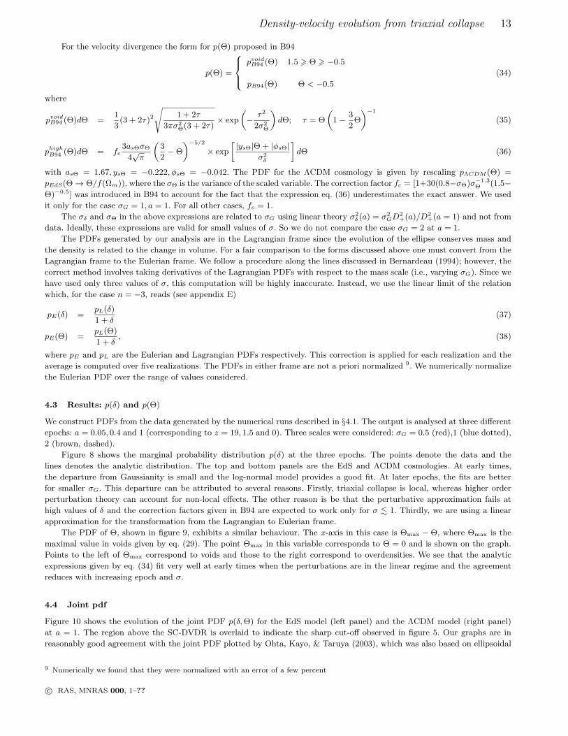
Figure 8 shows the marginal probability distribution p(δ) at the three epochs. The points denote the data and the

lines denotes the analytic distribution. The top and bottom panels are the EdS and ΛCDM cosmologies. At early times,

the departure from Gaussianity is small and the log-normal model provides a good fit. At later epochs, the fits are better

for smaller σG. This departure can be attributed to several reasons. Firstly, triaxial collapse is local, whereas higher order

perturbation theory can account for non-local effects. The other reason is be that the perturbative approximation fails at

high values of δ and the correction factors given in B94 are expected to work only for σ . 1. Thirdly, we are using a linear

approximation for the transformation from the Lagrangian to Eulerian frame.

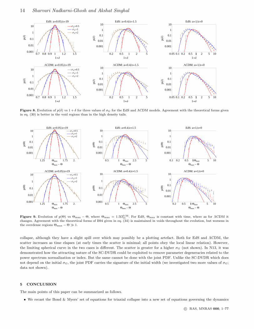
The PDF of Θ, shown in figure 9, exhibits a similar behaviour. The x-axis in this case is Θmax − Θ, where Θmax is the

maximal value in voids given by eq. (29). The point Θmax in this variable corresponds to Θ = 0 and is shown on the graph.

Points to the left of Θmax correspond to voids and those to the right correspond to overdensities. We see that the analytic

expressions given by eq. (34) fit very well at early times when the perturbations are in the linear regime and the agreement

reduces with increasing epoch and σ.

4.4 Joint pdf

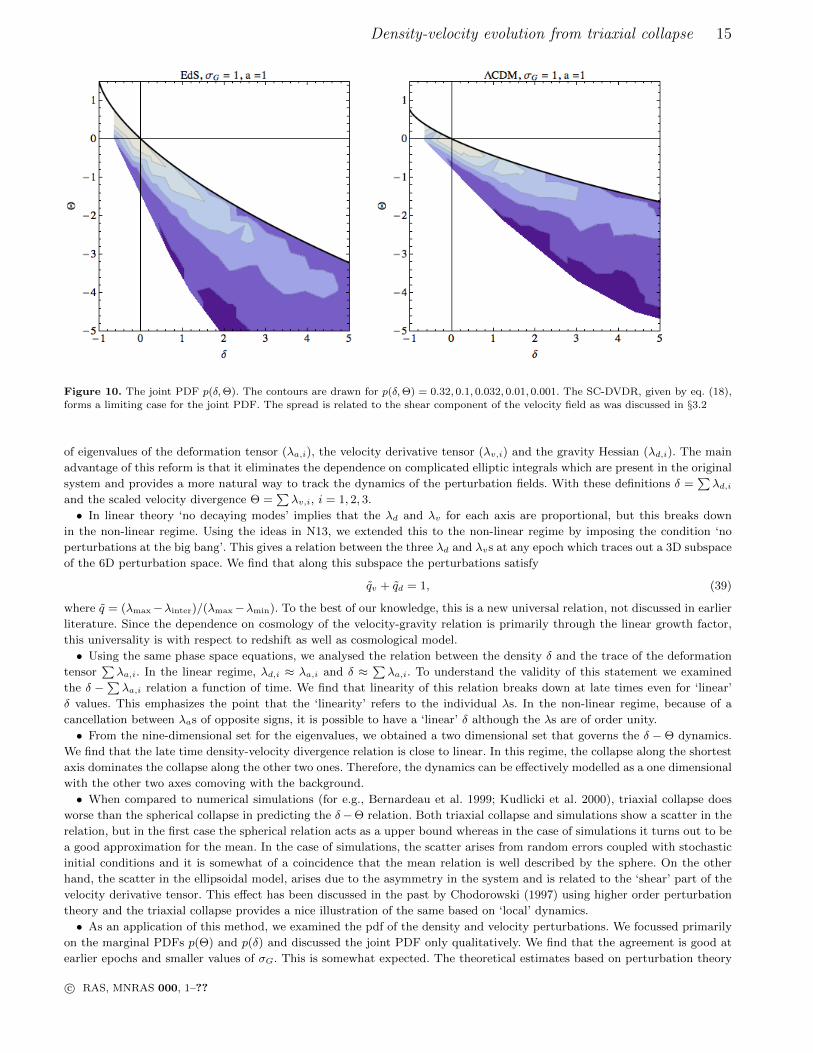
Figure 10 shows the evolution of the joint PDF p(δ,Θ) for the EdS model (left panel) and the ΛCDM model (right panel)

at a = 1. The region above the SC-DVDR is overlaid to indicate the sharp cut-off observed in figure 5. Our graphs are in

reasonably good agreement with the joint PDF plotted by Ohta, Kayo, & Taruya (2003), which was also based on ellipsoidal

9 Numerically we found that they were normalized with an error of a few percent

c© RAS, MNRAS 000, 1–??

14 Sharvari Nadkarni-Ghosh and Akshat Singhal

ΣG=0.5ΣG=1ΣG=2

0.7 0.8 0.9 1 1.2 1.50.001

0.01

0.1

1

10

1+∆

pH∆

LEdS: a=0.05z=19

0.2 0.5 1 2 5

0.001

0.01

0.1

1

10

1+∆

pH∆

L

EdS: a=0.4z=1.5

0.05 0.1 0.2 0.5 11 2 5 10

0.001

0.01

0.1

1

10

1+∆

pH∆

L

EdS: a=1z=0

ΣG=0.5ΣG=1ΣG=2

0.7 0.8 0.9 1 1.2 1.50.001

0.01

0.1

1

10

1+∆

pH∆

L

LCDM: a=0.05z=19

0.2 0.5 1 2 5

0.001

0.01

0.1

1

10

1+∆

pH∆

L

LCDM: a=0.4z=1.5

0.05 0.1 0.2 0.5 11 2 5 10

0.001

0.01

0.1

1

10

1+∆

pH∆

L

LCDM: a=1z=0

Figure 8. Evolution of p(δ) vs 1 + δ for three values of σG for the EdS and ΛCDM models. Agreement with the theoretical forms givenin eq. (30) is better in the void regions than in the high density tails.

ΣG=0.5ΣG=1ΣG=2

1.25 Qmax 1.75 2.

0.001

0.01

0.1

1

10

Qmax - Q

pHQ

L

EdS: a=0.05z=19

0.5 1 Qmax 2.5 5

0.001

0.01

0.1

1

10

Qmax - Q

pHQ

L

EdS: a=0.4z=1.5

0.1 0.2 0.5 11Qmax 5 10

0.001

0.01

0.1

1

10

Qmax - QpH

QL

EdS: a=1z=0

ΣG=0.5

ΣG=1

ΣG=2

1.25 Qmax 1.75 2.0.001

0.01

0.1

1

10

Qmax - Q

pHQ

L

LCDM: a=0.05z=19

0.5 1 Qmax 2.5 50.001

0.01

0.1

1

10

Qmax - Q

pHQ

L

LCDM: a=0.4z=1.5

0.2 0.5 11 Qmax 5 10

0.001

0.01

0.1

1

10

Qmax - Q

pHQ

L

LCDM: a=1z=0

Figure 9. Evolution of p(Θ) vs Θmax − Θ, where Θmax = 1.5Ω0.56m . For EdS, Θmax is constant with time, where as for ΛCDM it

changes. Agreement with the theoretical forms of B94 given in eq. (34) is maintained in voids throughout the evolution, but worsens in

the overdense regions Θmax −Θ 1.

collapse, although they have a slight spill over which may possibly be a plotting artefact. Both for EdS and ΛCDM, the

scatter increases as time elapses (at early times the scatter is minimal; all points obey the local linear relation). However,

the limiting spherical curve in the two cases is different. The scatter is greater for a higher σG (not shown). In N13, it was

demonstrated how the attracting nature of the SC-DVDR could be exploited to remove parameter degeneracies related to the

power spectrum normalization or index. But the same cannot be done with the joint PDF. Unlike the SC-DVDR which does

not depend on the initial σG, the joint PDF carries the signature of the initial width (we investigated two more values of σG;

data not shown).

5 CONCLUSION

The main points of this paper can be summarized as follows.

• We recast the Bond & Myers’ set of equations for triaxial collapse into a new set of equations governing the dynamics

c© RAS, MNRAS 000, 1–??

Density-velocity evolution from triaxial collapse 15

Figure 10. The joint PDF p(δ,Θ). The contours are drawn for p(δ,Θ) = 0.32, 0.1, 0.032, 0.01, 0.001. The SC-DVDR, given by eq. (18),

forms a limiting case for the joint PDF. The spread is related to the shear component of the velocity field as was discussed in §3.2

of eigenvalues of the deformation tensor (λa,i), the velocity derivative tensor (λv,i) and the gravity Hessian (λd,i). The main

advantage of this reform is that it eliminates the dependence on complicated elliptic integrals which are present in the original

system and provides a more natural way to track the dynamics of the perturbation fields. With these definitions δ =∑λd,i

and the scaled velocity divergence Θ =∑λv,i, i = 1, 2, 3.

• In linear theory ‘no decaying modes’ implies that the λd and λv for each axis are proportional, but this breaks down

in the non-linear regime. Using the ideas in N13, we extended this to the non-linear regime by imposing the condition ‘no

perturbations at the big bang’. This gives a relation between the three λd and λvs at any epoch which traces out a 3D subspace

of the 6D perturbation space. We find that along this subspace the perturbations satisfy

qv + qd = 1, (39)

where q = (λmax−λinter)/(λmax−λmin). To the best of our knowledge, this is a new universal relation, not discussed in earlier

literature. Since the dependence on cosmology of the velocity-gravity relation is primarily through the linear growth factor,

this universality is with respect to redshift as well as cosmological model.

• Using the same phase space equations, we analysed the relation between the density δ and the trace of the deformation

tensor∑λa,i. In the linear regime, λd,i ≈ λa,i and δ ≈

∑λa,i. To understand the validity of this statement we examined

the δ −∑λa,i relation a function of time. We find that linearity of this relation breaks down at late times even for ‘linear’

δ values. This emphasizes the point that the ‘linearity’ refers to the individual λs. In the non-linear regime, because of a

cancellation between λas of opposite signs, it is possible to have a ‘linear’ δ although the λs are of order unity.

• From the nine-dimensional set for the eigenvalues, we obtained a two dimensional set that governs the δ −Θ dynamics.

We find that the late time density-velocity divergence relation is close to linear. In this regime, the collapse along the shortest

axis dominates the collapse along the other two ones. Therefore, the dynamics can be effectively modelled as a one dimensional

with the other two axes comoving with the background.

• When compared to numerical simulations (for e.g., Bernardeau et al. 1999; Kudlicki et al. 2000), triaxial collapse does

worse than the spherical collapse in predicting the δ−Θ relation. Both triaxial collapse and simulations show a scatter in the

relation, but in the first case the spherical relation acts as a upper bound whereas in the case of simulations it turns out to be

a good approximation for the mean. In the case of simulations, the scatter arises from random errors coupled with stochastic

initial conditions and it is somewhat of a coincidence that the mean relation is well described by the sphere. On the other

hand, the scatter in the ellipsoidal model, arises due to the asymmetry in the system and is related to the ‘shear’ part of the

velocity derivative tensor. This effect has been discussed in the past by Chodorowski (1997) using higher order perturbation

theory and the triaxial collapse provides a nice illustration of the same based on ‘local’ dynamics.

• As an application of this method, we examined the pdf of the density and velocity perturbations. We focussed primarily

on the marginal PDFs p(Θ) and p(δ) and discussed the joint PDF only qualitatively. We find that the agreement is good at

earlier epochs and smaller values of σG. This is somewhat expected. The theoretical estimates based on perturbation theory

c© RAS, MNRAS 000, 1–??

16 Sharvari Nadkarni-Ghosh and Akshat Singhal

include non-local physics whereas the ellipsoidal model is local. In addition, the conversion from the Lagrangian frame to

Eulerian frame is based on a linear relation, which will breakdown for high values of δ. As another application we will consider

the evolution of axis ratios (paper II, Nadkarni-Ghosh & Singhal 2015).

The aim of this work was to understand the non-linear behaviour of density and velocity perturbations through the

eigenvalue dynamics. This work is general and gives rise to a range of possible applications. In particular, there is recent

interest in numerically classifying and quantifying the cosmic web based on eigenvalues of the gravity Hessian (Hahn et al.

2007; Forero-Romero et al. 2009) and the eigenvalues of the velocity derivative tensor (Hoffman et al. 2012; Libeskind, Hoffman,

& Gottlober 2014).One main issue in these studies is that the resultant mathematical structure depends not only on whether

one uses the gravitational tensor (T-web) or the velocity tensor (V-web), but it also depends on the details of the classification

algorithm (Hoffman et al. 2012; see Forero-Romero et al. 2014 for a list). Furthermore, it was also found that the velocity

based classification is a better tracer of the cosmic web and there have been independent observational evidences for the same

(Lee, Rey, & Kim 2014). However, the detailed reasoning based on a first principles analysis for this connection is unclear.

Through the newly defined ‘growth enhancement factor’ we are able to characterize the growth rates and provide an insight

into this result. Further investigations based on eigenvalue dynamics may help understand these numerical studies better.

Another possible application is to improve ellipsoidal collapse based mass function generating codes, such as PINOCCHIO

(Monaco et al. 2013). This will be useful to investigate the universal nature of mass function, dependence on cosmology etc.

Analytic descriptions of triaxial dynamics can also be used to resolve issues related to alignment or initial shapes of haloes

which have been raised in recent simulations (see for e.g. Despali, Tormen, & Sheth 2013) because time-reversing the phase

flow equations is easy making it possible to trace back to the initial conditions.

However, there are many limitations of the triaxial model considered here. The first important assumption is that the

principle axes stay fixed throughout the evolution i.e., no rotations are included. Second, the ellipse is isolated; the dynamics

is local. There are no interactions between neighbours. The effect of the environment is modelled through the effective external

non-linear tidal tensor, which depends completely on the axes lengths. The first extension of this analysis would be to follow

the more complete set of equations such as those given by Eisenstein & Loeb (1995), which includes rotation. Additional

parameters will be required to model the rotational degree of freedom, but the basic framework remains the same. The long-

term aim of such investigations would be to provide analytic insight that helps to interpret and improve numerical studies.

This paper presents a first step towards this goal.

6 ACKNOWLEDGEMENTS

We would like to thank the referee, Micha l Chodorowski, for his detailed comments and suggestions which improved the

original manuscript significantly. In addition, we would like to thank Sagar Chakraborty for useful discussions regarding

dynamical systems. S.N. would like to thank the hospitality of ICTP, Trieste, and discussions with Pierluigi Monaco and Ravi

Sheth which sowed the seeds of this work. Thanks are also due to Pierluigi Monaco for a careful reading of the manuscript

and valuable suggestions.

c© RAS, MNRAS 000, 1–??

Density-velocity evolution from triaxial collapse 17

REFERENCES

Angrick C., 2013, ArXiv e-prints, 1305, 497

Angrick C., Bartelmann M., 2010, Astronomy and Astrophysics, 518, 38

Audit E., Teyssier R., Alimi J.-M., 1997, Astronomy and Astrophysics, 325, 439

Bagla J. S., Padmanabhan T., 1996, The Astrophysical Journal, 469, 470

Bardeen J. M., Bond J. R., Kaiser N., Szalay A. S., 1986, The Astrophysical Journal, 304, 15

Bernardeau F., 1992, The Astrophysical Journal, 390, L61

Bernardeau F., 1994, Astronomy and Astrophysics, 291, 697

Bernardeau F., Chodorowski M. J., Lokas E. L., Stompor R., Kudlicki A., 1999, Monthly Notices of the Royal Astronomical

Society, 309, 543

Bernardeau F., Colombi S., Gaztaaga E., Scoccimarro R., 2002, Physics Reports, 367, 1

Bernardeau F., van de Weygaert R., 1996, Monthly Notices of the Royal Astronomical Society, 279, 693

Bernardeau F., van de Weygaert R., Hivon E., Bouchet F. R., 1997, Monthly Notices of the Royal Astronomical Society,

290, 566

Bilicki M., Chodorowski M. J., 2008, Monthly Notices of the Royal Astronomical Society, 391, 1796

Bonamigo M., Despali G., Limousin M., Angulo R., Giocoli C., Soucail G., 2014, arXiv:1410.0015 [astro-ph], arXiv: 1410.0015

Bond J. R., Myers S. T., 1996, Astrophysical Journal Supplement Series, 103, 1

Buchert T., 1992, Monthly Notices of the Royal Astronomical Society, 254, 729

Carlson B., 1987, Mathematics of Computation, 49, 595

Carlson B., 1989, Mathematics of Computation, 53, 327

Chodorowski M. J., 1997, Monthly Notices of the Royal Astronomical Society, 292, 695

Chodorowski M. J., Lokas E. L., 1997, Monthly Notices of the Royal Astronomical Society, 287, 591

Chodorowski M. J., Lokas E. L., Pollo A., Nusser A., 1998, Monthly Notices of the Royal Astronomical Society, 300, 1027

Ciecielag P., Chodorowski M. J., Kiraga M., Strauss M. A., Kudlicki A., Bouchet F. R., 2003, Monthly Notices of the Royal

Astronomical Society, 339, 641

Coles P., Jones B., 1991, Monthly Notices of the Royal Astronomical Society, 248, 1

Dekel A., Rees M. J., 1994, The Astrophysical Journal Letters, 422, L1

Del Popolo A., Ercan E. N., Xia Z., 2001, The Astronomical Journal, 122, 487

Del Popolo A., Gambera M., 2000, Astronomy and Astrophysics, 357, 809

Despali G., Tormen G., Sheth R. K., 2013, Monthly Notices of the Royal Astronomical Society, 431, 1143

Dodelson S., 2003, Modern Cosmology. Academic Press, Elsevier

Doroshkevich A. G., 1970, Astrophysics, 6, 320

Ehlers J., Buchert T., 1997, General Relativity and Gravitation, 29, 733

Eisenstein D. J., Loeb A., 1995, The Astrophysical Journal, 439, 520

Forero-Romero J. E., Contreras S., Padilla N., 2014, Monthly Notices of the Royal Astronomical Society, 443, 1090

Forero-Romero J. E., Hoffman Y., Gottlber S., Klypin A., Yepes G., 2009, Monthly Notices of the Royal Astronomical

Society, 396, 1815

Fosalba P., Gaztanaga E., 1998a, Monthly Notices of the Royal Astronomical Society, 301, 503

Fosalba P., Gaztanaga E., 1998b, Monthly Notices of the Royal Astronomical Society, 301, 535

Gramann M., 1993, The Astrophysical Journal Letters, 405, L47

Hahn O., Porciani C., Carollo C. M., Dekel A., 2007, Monthly Notices of the Royal Astronomical Society, 375, 489

Hoffman Y., Metuki O., Yepes G., Gottlober S., Forero-Romero J. E., Libeskind N. I., Knebe A., 2012, Monthly Notices of

the Royal Astronomical Society, 425, 2049, arXiv: 1201.3367

Icke V., 1973, Astronomy and Astrophysics, 27, 1

Johnson A. et al., 2014, Monthly Notices of the Royal Astronomical Society, 444, 3926

Joyce M., Marcos B., Baertschiger T., 2009, Monthly Notices of the Royal Astronomical Society, 394, 751

Joyce M., Sylos Labini F., 2012, ArXiv e-prints, 1210, 1140

Kayo I., Taruya A., Suto Y., 2001, The Astrophysical Journal, 561, 22

Kerscher M., Buchert T., Futamase T., 2001, The Astrophysical Journal, 558, 79

Kitaura F.-S., Angulo R. E., Hoffman Y., Gottlber S., 2012, Monthly Notices of the Royal Astronomical Society, 425, 2422

Kitaura F.-S., Heß S., 2013, Monthly Notices of the Royal Astronomical Society, 435, L78

Kofman L., Bertschinger E., Gelb J. M., Nusser A., Dekel A., 1994, The Astrophysical Journal, 420, 44

Kudlicki A., Chodorowski M., Plewa T., Ryczka M., 2000, Monthly Notices of the Royal Astronomical Society, 316, 464

Lam T. Y., Sheth R. K., 2008a, Monthly Notices of the Royal Astronomical Society, 389, 1249

Lam T. Y., Sheth R. K., 2008b, Monthly Notices of the Royal Astronomical Society, 386, 407

Lee J., Rey S. C., Kim S., 2014, The Astrophysical Journal, 791, 15

c© RAS, MNRAS 000, 1–??

18 Sharvari Nadkarni-Ghosh and Akshat Singhal

Libeskind N. I., Hoffman Y., Gottlober S., 2014, Monthly Notices of the Royal Astronomical Society, 441, 1974

Lin C. C., Mestel L., Shu F. H., 1965, The Astrophysical Journal, 142, 1431

Linder E. V., 2005, Physical Review D, 72, 43529

Lokas E. L., 2000, Monthly Notices of the Royal Astronomical Society, 311, 423

Lynden-Bell D., 1964, The Astrophysical Journal, 139, 1195

Majerotto E. et al., 2012, Monthly Notices of the Royal Astronomical Society, 424, 1392

Martino M. C., Stabenau H. F., Sheth R. K., 2009, Physical Review D, 79, 84013

Matarrese S., Pietroni M., 2007, Journal of Cosmology and Astro-Particle Physics, 06, 026

Matsubara T., 2008, Physical Review D, 77, 63530

Monaco P., 1995, The Astrophysical Journal, 447, 23

Monaco P., Sefusatti E., Borgani S., Crocce M., Fosalba P., Sheth R. K., Theuns T., 2013, Monthly Notices of the Royal

Astronomical Society, 433, 2389

Monaco P., Theuns T., Taffoni G., 2002, Monthly Notices of the Royal Astronomical Society, 331, 587

Nadkarni-Ghosh S., 2013, Monthly Notices of the Royal Astronomical Society, 428, 1166

Nadkarni-Ghosh S., Chernoff D. F., 2011, Monthly Notices of the Royal Astronomical Society, 410, 1454

Nadkarni-Ghosh S., Chernoff D. F., 2013, Monthly Notices of the Royal Astronomical Society, 431, 799

Nadkarni-Ghosh S., Singhal A., 2015, ArXiv e-prints, 1501, 7075

Nariai H., Fujimoto M., 1972, Progress of Theoretical Physics, 47, 105

Navarro J. F., Frenk C. S., White S. D. M., 1996, The Astrophysical Journal, 462, 563

Nusser A., Dekel A., Bertschinger E., Blumenthal G. R., 1991, The Astrophysical Journal, 379, 6

Ohta Y., Kayo I., Taruya A., 2003, The Astrophysical Journal, 589, 1

Ohta Y., Kayo I., Taruya A., 2004, The Astrophysical Journal, 608, 647

Peebles P., 1980, The Large-Scale Structure of the Universe. Princeton University Press

Press W., Teukolsky S., Vetterling W., Flannery B., 2002, Numerical Recipes in C++. Cambridge University Press

Press W. H., Schechter P., 1974, Astrophysical Journal, 187, 425

Rossi G., 2012, Monthly Notices of the Royal Astronomical Society, 421, 296

Scherrer R. J., Gaztaaga E., 2001, Monthly Notices of the Royal Astronomical Society, 328, 257

Schneider M. D., Frenk C. S., Cole S., 2012, Journal of Cosmology and Astro-Particle Physics, 05, 030

Sheth R. K., Mo H. J., Tormen G., 2001, Monthly Notices of the Royal Astronomical Society, 323, 1

Stabenau H. F., Jain B., 2006, Physical Review D, 74, 84007

Susperregi M., Buchert T., 1997, Astronomy and Astrophysics, 323, 295

White S. D. M., Silk J., 1979, Astrophysical Journal, 231, 1

Wintergerst N., Pettorino V., 2010, Physical Review D, 82, 103516

Zeldovich Y. B., 1970, Astronomy and Astrophysics, 5, 84

APPENDIX A: DEFINITIONS OF THE TENSORS

The physical and comoving axes of the ellipse are

ri = aiqi xi =aiaqi, (A1)

where qi is the initial Lagrangian coordinate of the i-th axis. Initially, the ai are different from a, so qi is not the initial

comoving coordinate. If we want to characterize the deformation from the sphere then for the sphere q1 = q2 = q3. The

deformation and velocity are

si = qi − xi =(

1− aia

)qi (A2)

vi = ri −Hri =

(aiai−H

)ri. (A3)

The deformation tensor is

eij =1

2

(∂si∂qj

+∂sj∂qi

)= λa,iδij . (A4)

Note that we differ from BM96 by a minus sign. However, their relevant eigenvalues (denoted as λv,A) are negative of the

eigenvalues of their eij . We have expressed it so that the λa are eigenvalues of eij . This is just a matter of convention. The

important point is that in both conventions λa = λd in the linear regime and∑λa,i = δ. The tensor of velocity derivatives is

1

2H

(∂vi∂rj

+∂vj∂ri

)= λv,iδij . (A5)

c© RAS, MNRAS 000, 1–??

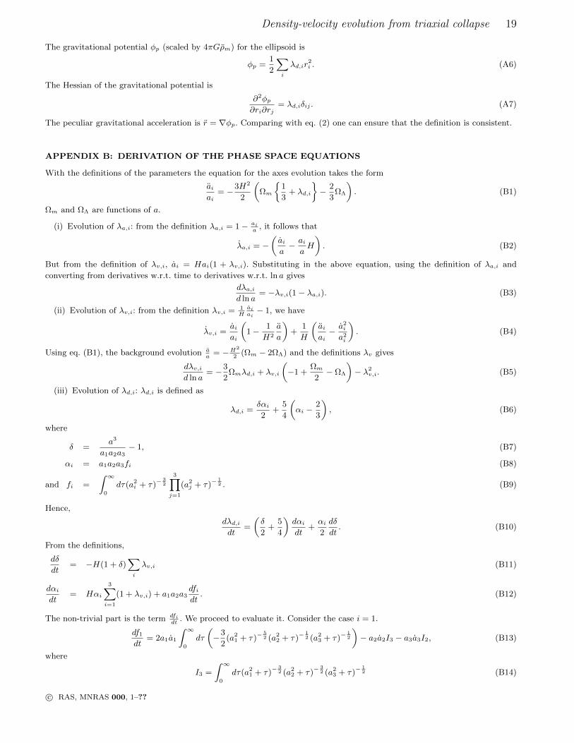
Density-velocity evolution from triaxial collapse 19

The gravitational potential φp (scaled by 4πGρm) for the ellipsoid is

φp =1

2

∑i

λd,ir2i . (A6)

The Hessian of the gravitational potential is

∂2φp∂ri∂rj

= λd,iδij . (A7)

The peculiar gravitational acceleration is r = ∇φp. Comparing with eq. (2) one can ensure that the definition is consistent.

APPENDIX B: DERIVATION OF THE PHASE SPACE EQUATIONS

With the definitions of the parameters the equation for the axes evolution takes the form

aiai

= −3H2

2

(Ωm

1

3+ λd,i

− 2

3ΩΛ

). (B1)

Ωm and ΩΛ are functions of a.

(i) Evolution of λa,i: from the definition λa,i = 1− aia

, it follows that

λa,i = −(aia− aiaH

). (B2)

But from the definition of λv,i, ai = Hai(1 + λv,i). Substituting in the above equation, using the definition of λa,i and

converting from derivatives w.r.t. time to derivatives w.r.t. ln a gives

dλa,id ln a

= −λv,i(1− λa,i). (B3)

(ii) Evolution of λv,i: from the definition λv,i = 1Haiai− 1, we have

λv,i =aiai

(1− 1

H2

a

a

)+

1

H

(aiai− a2

i

a2i

). (B4)

Using eq. (B1), the background evolution aa

= −H2

2(Ωm − 2ΩΛ) and the definitions λv gives

dλv,id ln a

= −3

2Ωmλd,i + λv,i

(−1 +

Ωm2− ΩΛ

)− λ2

v,i. (B5)

(iii) Evolution of λd,i: λd,i is defined as

λd,i =δαi2

+5

4

(αi −

2

3

), (B6)

where

δ =a3

a1a2a3− 1, (B7)

αi = a1a2a3fi (B8)

and fi =

∫ ∞0

dτ(a2i + τ)−

32

3∏j=1

(a2j + τ)−

12 . (B9)

Hence,

dλd,idt

=

(δ

2+

5

4

)dαidt

+αi2

dδ

dt. (B10)

From the definitions,

dδ

dt= −H(1 + δ)

∑i

λv,i (B11)

dαidt

= Hαi

3∑i=1

(1 + λv,i) + a1a2a3dfidt. (B12)

The non-trivial part is the term dfidt

. We proceed to evaluate it. Consider the case i = 1.

df1

dt= 2a1a1

∫ ∞0

dτ

(−3

2(a2

1 + τ)−52 (a2

2 + τ)−12 (a2

3 + τ)−12

)− a2a2I3 − a3a3I2, (B13)

where

I3 =

∫ ∞0

dτ(a21 + τ)−

32 (a2

2 + τ)−32 (a2

3 + τ)−12 (B14)

c© RAS, MNRAS 000, 1–??

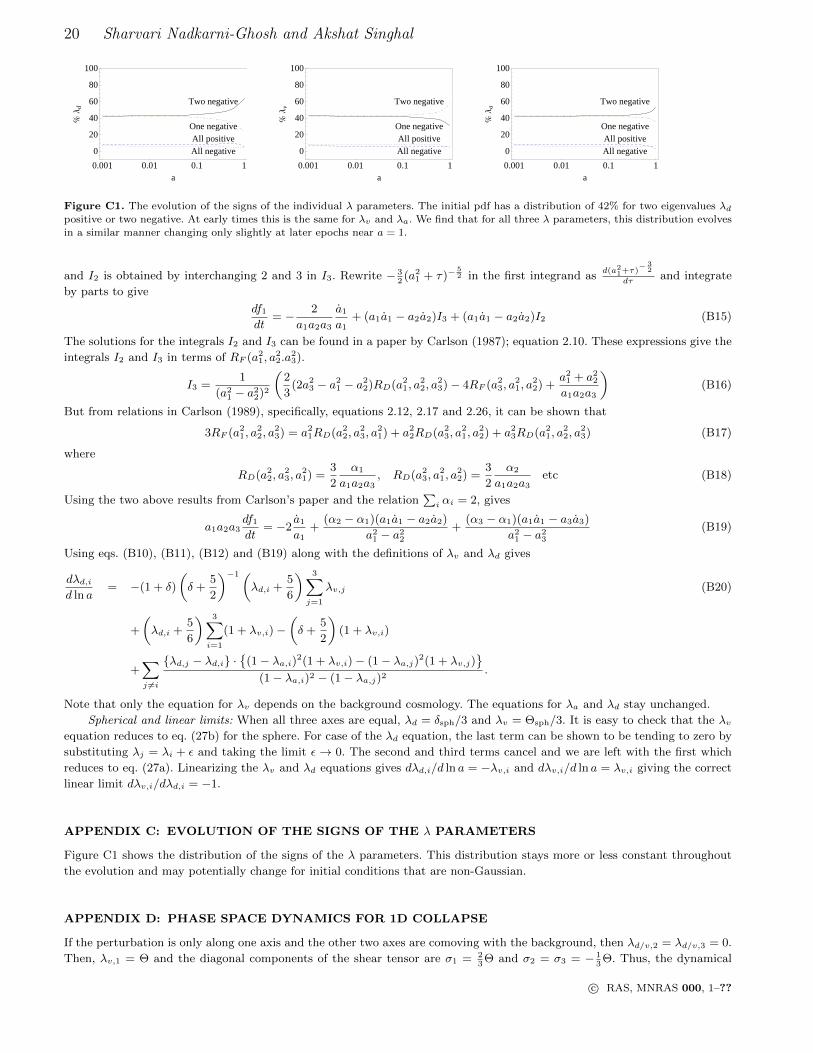
20 Sharvari Nadkarni-Ghosh and Akshat Singhal

All positiveAll negative

One negative

Two negative

0.001 0.01 0.1 1

0

20

40

60

80

100

a

%Λ

d

All positiveAll negative

One negative

Two negative

0.001 0.01 0.1 1

0

20

40

60

80

100

a

%Λ

v

All positiveAll negative

One negative

Two negative

0.001 0.01 0.1 1

0

20

40

60

80

100

a

%Λ

a

Figure C1. The evolution of the signs of the individual λ parameters. The initial pdf has a distribution of 42% for two eigenvalues λdpositive or two negative. At early times this is the same for λv and λa. We find that for all three λ parameters, this distribution evolves

in a similar manner changing only slightly at later epochs near a = 1.

and I2 is obtained by interchanging 2 and 3 in I3. Rewrite − 32(a2

1 + τ)−52 in the first integrand as

d(a21+τ)− 3

2

dτand integrate

by parts to give

df1

dt= − 2

a1a2a3

a1

a1+ (a1a1 − a2a2)I3 + (a1a1 − a2a2)I2 (B15)

The solutions for the integrals I2 and I3 can be found in a paper by Carlson (1987); equation 2.10. These expressions give the

integrals I2 and I3 in terms of RF (a21, a

22.a

23).

I3 =1

(a21 − a2

2)2

(2

3(2a2

3 − a21 − a2

2)RD(a21, a

22, a

23)− 4RF (a2

3, a21, a

22) +

a21 + a2

2

a1a2a3

)(B16)

But from relations in Carlson (1989), specifically, equations 2.12, 2.17 and 2.26, it can be shown that

3RF (a21, a

22, a

23) = a2

1RD(a22, a

23, a

21) + a2

2RD(a23, a

21, a

22) + a2

3RD(a21, a

22, a

23) (B17)

where

RD(a22, a

23, a

21) =

3

2

α1

a1a2a3, RD(a2

3, a21, a

22) =

3

2

α2

a1a2a3etc (B18)

Using the two above results from Carlson’s paper and the relation∑i αi = 2, gives

a1a2a3df1

dt= −2

a1

a1+

(α2 − α1)(a1a1 − a2a2)

a21 − a2

2

+(α3 − α1)(a1a1 − a3a3)

a21 − a2

3

(B19)

Using eqs. (B10), (B11), (B12) and (B19) along with the definitions of λv and λd gives

dλd,id ln a

= −(1 + δ)

(δ +

5

2

)−1(λd,i +

5

6

) 3∑j=1

λv,j (B20)

+

(λd,i +

5

6

) 3∑i=1

(1 + λv,i)−(δ +

5

2

)(1 + λv,i)

+∑j 6=i

λd,j − λd,i ·

(1− λa,i)2(1 + λv,i)− (1− λa,j)2(1 + λv,j)

(1− λa,i)2 − (1− λa,j)2.

Note that only the equation for λv depends on the background cosmology. The equations for λa and λd stay unchanged.

Spherical and linear limits: When all three axes are equal, λd = δsph/3 and λv = Θsph/3. It is easy to check that the λvequation reduces to eq. (27b) for the sphere. For case of the λd equation, the last term can be shown to be tending to zero by

substituting λj = λi + ε and taking the limit ε → 0. The second and third terms cancel and we are left with the first which

reduces to eq. (27a). Linearizing the λv and λd equations gives dλd,i/d ln a = −λv,i and dλv,i/d ln a = λv,i giving the correct

linear limit dλv,i/dλd,i = −1.

APPENDIX C: EVOLUTION OF THE SIGNS OF THE λ PARAMETERS

Figure C1 shows the distribution of the signs of the λ parameters. This distribution stays more or less constant throughout

the evolution and may potentially change for initial conditions that are non-Gaussian.

APPENDIX D: PHASE SPACE DYNAMICS FOR 1D COLLAPSE

If the perturbation is only along one axis and the other two axes are comoving with the background, then λd/v,2 = λd/v,3 = 0.

Then, λv,1 = Θ and the diagonal components of the shear tensor are σ1 = 23Θ and σ2 = σ3 = − 1

3Θ. Thus, the dynamical

c© RAS, MNRAS 000, 1–??

Density-velocity evolution from triaxial collapse 21

system given by eq. (26) for an EdS cosmology reduces to

dδ

d ln a= −(1 + δ)Θ (D1a)

dΘ

d ln a= −1

2

[3δ + Θ + 2Θ2] , (D1b)

Rearrange the terms in the second equation (add and subtract δ and express Θ = 3Θ− 2Θ) to give

dΘ

d ln a= (1 + δ)Θ− (Θ + δ)(3 + 2Θ)

2. (D2)

Dividing the second equation by the first, gives

dΘ

dδ= −1 +

(Θ + δ)(3 + 2Θ)

2Θ(1 + δ)(D3)

It is easy to check that a linear relation satisfies this equation. The initial conditions are Θ(δ = 0) = 0 and dΘdδ

∣∣δ=0

= c, where

c is some pre-determined constant. Let Θ = Aδ+B be a solution to the above equation with the given initial conditions. The

first initial condition sets B = 0 and the second one gives

dΘ

dδ

∣∣∣∣δ=0

= −1 +3

2(A+ 1) = c, (D4)

which in turn sets A = 23(1 + c)− 1. For c = −1, A = −1 giving Θ = −δ. A similar argument will hold for the ΛCDM case:

only the coefficient of Θ changes so the rearrangement of terms will be slightly different and the constant c (or alternatively

A) will involve some factors of Ωm and ΩΛ.

APPENDIX E: RELATION BETWEEN THE LAGRANGIAN AND EULERIAN PDFS

Given a discrete distribution of massive particles with a mean density ρ there are two ways to define the density field. At each

point, consider the amount of matter M contained in a fixed volume V0 and define the density contrast as δ(M,V0) = 1ρMV0

.

This corresponds to the Eulerian prescription. Alternately, in the Lagrangian prescription, at each point one estimates the

volume occupied by a fixed mass M0 and the corresponding density contrast is δ = 1ρM0V

. M0 and V0 are related through δ0as

δ0 =1

ρ

M0

V0− 1. (E1)

In the Eulerian prescription, δ and M are equivalent variables whereas in the Lagrangian prescription, δ and V are equivalent.

Furthermore, a different choice of V0 for the same choice of M0 gives a different Eulerian density field and similarly a different

choice of M0 for a fixed choice of V0 gives a different Lagrangian density field. To relate the PDFs of the Eulerian and

Lagrangian fields, note that the probability that a given volume V0 contains an amount of matter greater than M0 is same as

the probability that M0 occupies a volume smaller than V0 (B94 page 702, eq. 33a). This gives∫ ∞M0

pE(V0,M)dM =

∫ V0

0

pL(V,M0)dV. (E2)

To change the integration variable to δ note that

pE(V0,M) = pE(V0, δ)

∣∣∣∣ dδdM∣∣∣∣ =⇒ pE(V0,M)dM = pE(V0, δ)dδ (E3)

pL(V,M0) = pL(δ,M0)

∣∣∣∣ dδdV∣∣∣∣ =⇒ pL(V,M0)dV = −pL(δ,M0)dδ. (E4)

The negative sign arises in the second equation because δ and V are inversely related. The end points of the first intergal:

M = M0,∞ =⇒ δ = δ0,∞ and in the second V = 0, V0 =⇒ δ = ∞, δ0. Thus, eq. (E2) becomes∫ ∞δ0

pE(V0, δ)dδ =

∫ ∞δ0

pL(δ,M0)dδ. (E5)

Differentiating w.r.t. δ0 for a fixed V0 gives

−pE(V0, δ0) = −pL(δ0,M0) +

∫ δ0

∞

∂

∂δ0pL(δ,M0)dδ

. (E6)

The above relation is between the discrete Eulerian and Lagrangian densities. Using the relation between the smooth and

discrete densities given by B94 (i.e., the PDFs of the Eulerian densities differ by 1 + δ, where as the PDFs of the Lagrangian

densities are the same) gives

(1 + δ0)pE(V0, δ0) =

pL(δ0,M0)−

∫ ∞δ0

∂

∂δ0pL(δ,M0)dδ.

. (E7)

c© RAS, MNRAS 000, 1–??

22 Sharvari Nadkarni-Ghosh and Akshat Singhal

The second term on the r.h.s. depends on the variation of pL with δ0 or alternately M0. Ideally, to compute it we need to

know how pL varies with M0. A different mass scale corresponds to a different choice of σ. So we can rewrite

∂pL∂δ0

=∂pLdM0

∂M0

dδ0(E8)

=∂pLdσ

∂σ

∂M0

∂M0

∂δ0(E9)

=∂pLdσ

∂σ

∂Rf

∂Rf∂δ0

, (E10)

where in the last equality we have introduced the filtering scale Rf which corresponds to the mass scale M0 through

M0 =4

3πR3

f ρ. (E11)

Combining the above with eq. (E1),

(1 + δ0)V0 =4

3πR3

f (E12)

and differentiating w.r.t. δ0 at a fixed V0 gives

dRfdδ0

=Rf

3(1 + δ0). (E13)

Since dσdRf

anddRfdδ0

do not depend on δ, eq. (E7) becomes

(1 + δ0)pE(V0, δ0) =

pL(δ0, σ)− dσ

dRf

dRfdδ0

∫ ∞δ0

dpL(δ, σ)

dσdδ.

. (E14)

In eq. (E14), pL corresponds to the non-linear probability distribution, however, the numerical studies in this paper were

performed with only a few values of σ and the dependence of the distribution on σ cannot be known accurately. Instead, we

examine the linear limit to obtain an analytic result and extend the result to the quasi-linear regime. This procedure can be

partially justified by arguing that the theoretical results of B94 (the Eulerian pdf that we compare with) are expected to be

valid only for small σ.

In the linear regime,

pL(δ) =1√2πσ

exp

(− δ2

2σ2

). (E15)

dpLdσ

= − 1√2πσ2

exp

(− δ2

2σ2

)+

δ2

√2πσ4

exp

(− δ2

2σ2

). (E16)

and the integral becomes ∫ ∞δ0

dpL(δ, σ)

dσdδ =

e−δ202σ2 δ0√2πσ2

=δ0σpL. (E17)

It remains to compute dσdRf

in eq. (E14). This depends on the power spectrum and the window function.

σ2(Rf ) =

∫P (k)W 2(kRf )d3k (E18)

Assuming a Gaussian filter W (kRf ) = exp− k2R2

f

2and a power spectrum with index n i.e., P (k) = c0k

n, where c0 is some

constant,

σ2 =c02R−(n+3)f Γ

(n+ 3

2

); 2σ

dσ

dRf= −n+ 3

Rfσ2 (E19)

and

dσ

dRf= − (n+ 3)

2

σ

Rf. (E20)

Putting together eqs. (E13), (E14), (E17) and (E20), gives

(1 + δ0)pE = pL

[1 +

(n+ 3)

6

δ01 + δ0

]. (E21)

In our comparisons, we used n = −3. In this case, σ is independent of the smoothing scale and the relation is simply

pE(δ0) =pL(δ0)

1 + δ0. (E22)

Arguing that the density-velocity divergence relation is the same in both frames (mean velocity divergence is computed from

c© RAS, MNRAS 000, 1–??

Density-velocity evolution from triaxial collapse 23

the velocity field (within a fixed volume in the Eulerian case and within a fixed mass in the Lagrangian case), the velocity

PDFs also have the same relation:

pE(Θ) =pL(Θ)

1 + δ. (E23)

The Eulerian PDFs predicted by our analysis and the ones used for comparison are both normalized numerically.

c© RAS, MNRAS 000, 1–??