
ADAPTIVE VIRTUAL ENVIRONMENTS IN MODERN MULTI-PLAYER
COMPUTER GAMES
by
Marc Lanctot
School of Computer Science
McGill University, Montreal
February 2005
A thesis submitted to McGill University
in partial fulfillment of the requirements of the degree of
Master of Science
Copyright c© 2005 by Marc Lanctot

Abstract
Most modern computer games provide a virtual environment as a context for player inter-
action. Recently, many multi-player online games have adopted the persistent-state gaming
model, which provides a central virtual environment with essentially infinite lifetime. How-
ever, a displeasing part of these long-lasting environments is that, like their predecessors, they
are still assumed to be static, unchanging even in the long-term. In response to this fact, we
introduce the adaptive virtual environment which automatically adapts based on activity occur-
ring within the environment. In computer games, adaptive virtual environments are systems
that correspond to real-world physical or social systems. These systems are computationally
formalized by adhering to a generic adaptation model containing abstract components and pro-
cedures. Herein, as a proof of concept, we design and analyze the behavior of two adaptive
versions of such systems commonly found in persistent-state games. To achieve this, we build
an implementation of an abstract interactive simulator that applies the adaptation process to
our example systems. Each system is internally represented as a plug-in module containing
system-specific implementations of the model’s abstractly-defined procedures. Performance of
the adaptation process is then evaluated using simulation data. Finally, improvements such
as optimizations and better movement models for agent simulation are investigated, and the
general usefulness and applicability of the concepts is discussed.
i

Resume
La plupart des jeux informatiques modernes offrent aux joueurs un environnement virtuel
qui leur permet d’interagir entre eux. Recemment, plusieurs jeux multi-joueurs en-ligne ont
adopte un modele de jeu avec etat persistant qui fournit un environnement virtuel central et
dont le temps de vie est quasi-infini. Ces nouveaux environnements ont tout de meme herite du
meme probleme que leurs predecesseurs : on les considere comme etant statiques c’est-a-dire
qu’ils ne changent pas avec le temps, meme a long terme. Considerant ce fait, nous presentons
l’environnement virtuel adaptable qui s’ajuste automatiquement en fonction des evenements qui
se deroulant dans l’environnement. Pour les jeux video, les environnements virtuels adaptables
sont des reproductions de notre monde physique ou social. Ces systemes sont formalizes en
respectant un modele d’adaptation generique qui contient des des procedures et modules ab-
straits. Afin de demontrer cette formalisation, nous avons elabore et analyse le comportement
de deux versions adaptables de systemes couramment retrouves dans des jeux a etat persistant.
Pour y parvenir, nous avons construit un simulateur interactif abstrait qui qui met en appli-
cation le processus d’adaptation dans chacun de nos deux systemes temoins. Chaque systeme
analyse par notre simulateur est represente par un module d’ajout (plug-in) qui contient le
comportement des methodes abstraites specifiques a ce systeme. La performance du processus
d’adaptation est alors evaluee avec des donnees de simulation. Finalement, des ameliorations,
telles que des optimisations et des modeles de mouvement perfectionnes pour la simulation
d’agents sont etudiees. L’utilite de ce concept et ses debouches sont egalement discutees.
ii

Acknowledgments
I would especially like to thank my thesis supervisor, Clark Verbrugge, for his patience,
support, encouragement and guidance. When I had lost hope while experimenting, his belief
in my research and persistence motivated me to continue. For everything he has given, he has
earned my utmost respect.
As well, I’d like to thank the professors in charge of the Sable research lab (Clark Verbrugge
and Laurie Hendren) for providing me with a research assistantship that not only paid for in
part the costs associated with this research, but also allowed me to develop basic system ad-
ministration skills. In addition, the Sable lab provided a great study environment and powerful
machines for performance and concurrency analysis.
I would also like to thank the McGill School of Computer Science, in particular Alex Batko
who was very responsive and helpful in the organizing of the Conquero game-playing experi-
ment, the administration who have always been more than helpful, and all the faculty members
who put their painstaking effort into teaching for the sake of the advancement of academia; they
are true role models, and as such have all helped contribute in a small way. Thanks to everyone
who helped out with the translation of the abstract: Alexandre Denault, Marc Boscher, Eric-
Oliver Lamey, Olivier Abbe, Patrick Desnoyers, and Marc Gendron-Bellemare. Special thanks
goes to Alexandre Denault for inspiring Conquero providing the Minueto game framework along
with support for it. Of course, thanks goes to all the participants that made the experiment
possible. This includes but is not restricted to: Francis Perron, Julia Grav, Alexandre Denault,
Sokhom Pheng, Marc “mini-marc” Gendron-Bellemare, Kacper Wysocki, Olivier Hebert, De-
nis Lebel, Felix Martineau, Francois Poirier, Julien Vanier, Duc-Duy Nguyen, Jean-Sebastien
Legare, Raphael Bouskila, David Moise Nataf, Ali “Rushie” Rushdan Tariq, Ivaylo Tzvetkov,
Mathieu Guay-Paquet, Zhentao Li, and Craig Hooker.
Finally I’d like to thank Nancy Forget, my parents and family, and the rest of my friends
who have by now been hearing the sentence “I can’t, I have to work on my thesis” for too long.
Their tolerance has been well-appreciated.
Thank you, everyone, for your help and understanding.
iii

Contents
Abstract i
Resume ii
Acknowledgments iii
Contents iv
List of Figures vi
List of Tables viii
1 Introduction and Contributions 1
1.1 Contributions . . . . . . . . . . . . . . . . . . . . . . . . . . . . . . . . . . . . . 3
1.2 Road map . . . . . . . . . . . . . . . . . . . . . . . . . . . . . . . . . . . . . . . 3
2 Related Work 4
2.1 Adaptation . . . . . . . . . . . . . . . . . . . . . . . . . . . . . . . . . . . . . . 4
2.2 Cellular Automata . . . . . . . . . . . . . . . . . . . . . . . . . . . . . . . . . . 5
2.3 Fuzzy Logic and Fuzzy Set Theory . . . . . . . . . . . . . . . . . . . . . . . . . 6
2.4 Ecological(Weather) Modeling and Simulation . . . . . . . . . . . . . . . . . . . 6
2.5 Reputation Systems . . . . . . . . . . . . . . . . . . . . . . . . . . . . . . . . . . 7
2.6 Multi-player Game Design . . . . . . . . . . . . . . . . . . . . . . . . . . . . . . 8
2.7 Terrain Generation . . . . . . . . . . . . . . . . . . . . . . . . . . . . . . . . . . 9
3 A General Model for Adaptive Environments 10
3.1 Fundamental Notions . . . . . . . . . . . . . . . . . . . . . . . . . . . . . . . . . 10
3.1.1 Cellular Automata . . . . . . . . . . . . . . . . . . . . . . . . . . . . . . 11
3.1.2 Fuzzy Control . . . . . . . . . . . . . . . . . . . . . . . . . . . . . . . . . 13
3.2 Basics of the Adaptation Model . . . . . . . . . . . . . . . . . . . . . . . . . . . 17
iv

3.2.1 Generic Adaptation Procedures . . . . . . . . . . . . . . . . . . . . . . . 21
4 Applications of the Model 27
4.1 Environment-based Applications . . . . . . . . . . . . . . . . . . . . . . . . . . . 28
4.1.1 An Adaptive Weather System . . . . . . . . . . . . . . . . . . . . . . . . 28
4.2 Agent-based Applications . . . . . . . . . . . . . . . . . . . . . . . . . . . . . . 41
4.2.1 An Adaptive Reputation System . . . . . . . . . . . . . . . . . . . . . . 42
5 Movement Models for Mobile Agents 50
5.1 Conquero . . . . . . . . . . . . . . . . . . . . . . . . . . . . . . . . . . . . . . . 51
5.2 Game-playing Experiment . . . . . . . . . . . . . . . . . . . . . . . . . . . . . . 53
5.3 Building a Movement Model . . . . . . . . . . . . . . . . . . . . . . . . . . . . . 54
5.3.1 Classification and Statistical Learning . . . . . . . . . . . . . . . . . . . 57
5.3.2 Learning How to Move in a Dynamic Environment . . . . . . . . . . . . 62
5.4 Other Movement Models . . . . . . . . . . . . . . . . . . . . . . . . . . . . . . . 65
5.5 Applying the Models to Agent-based Adaptation . . . . . . . . . . . . . . . . . 65
6 An Implementation of the Adaptation Framework 69
6.1 Adaptation in Modern Persistent-state Games . . . . . . . . . . . . . . . . . . . 69
6.2 Design and Implementation of the Adaptation Engine . . . . . . . . . . . . . . . 71
6.3 Performance Measurements . . . . . . . . . . . . . . . . . . . . . . . . . . . . . 79
6.4 Optimizations . . . . . . . . . . . . . . . . . . . . . . . . . . . . . . . . . . . . . 85
6.4.1 Caching . . . . . . . . . . . . . . . . . . . . . . . . . . . . . . . . . . . . 85
6.4.2 Concurrency . . . . . . . . . . . . . . . . . . . . . . . . . . . . . . . . . . 86
6.4.3 Buffering . . . . . . . . . . . . . . . . . . . . . . . . . . . . . . . . . . . . 89
6.4.4 Aggregation . . . . . . . . . . . . . . . . . . . . . . . . . . . . . . . . . . 90
7 Future Work and Conclusions 92
7.1 Future Work . . . . . . . . . . . . . . . . . . . . . . . . . . . . . . . . . . . . . . 94
Appendices
A Learned Decision Tree 97
Bibliography 113
v

List of Figures
3.1 Evolution (Ct vs. t) for a simple CA example. . . . . . . . . . . . . . . . . . . . . 12
3.2 The effects of one iteration in Game of Life. . . . . . . . . . . . . . . . . . . . . . 12
3.3 The graph of the membership function, µTALL(x), vs x for the fuzzy set “x is TALL”. 14
3.4 (a) The region produced by center-of-gravity defuzzification in a fuzzy controller with
an action set containing 3 overlapping fuzzy actions, and (b) The center of gravity,
and the chosen (red) action. . . . . . . . . . . . . . . . . . . . . . . . . . . . . . . 16
3.5 The virtual terrain. . . . . . . . . . . . . . . . . . . . . . . . . . . . . . . . . . . 17
3.6 The effects of one iteration of blurring on a letter image, A letter is displayed closeup
(a) before and (b) after the blurring of the image. . . . . . . . . . . . . . . . . . . 19
3.7 The effects of one iteration of blurring on a dragon image. A dragon is displayed (a)
before and (b) after the blurring of the image. . . . . . . . . . . . . . . . . . . . . 20
3.8 The causal block diagram representing the general adaptation process. . . . . . . . . 21
3.9 A region affected by modifications after 1 timestep of blurring using (a) sequential
iterative updates and (b) simultaneous update rules . . . . . . . . . . . . . . . . . 22
3.10 Affect of an update on one grid section (assuming γ = 1), showing a) before the change
b) before the update on the middle grid section c) after the change and update . . . . 23
4.1 Example gradient vector representation. Grid cells show local terrain altitudes. . . . 30
4.2 Example of degenerate cases where (a) ~vgrad = 0 and (b) ~vwind avg = 0. . . . . . . . 31
4.3 An example of obtaining ~vtarget given ~vgrad, ~vwind avg, and α = 0.8 . . . . . . . . . . 32
4.4 An example weather system configuration after several hundred iterations showing
wind and altitude values. Bright red areas are high (land/mountains), black areas are
low (seas), and the arrows show the direction of wind movement. . . . . . . . . . . . 33
4.5 An example weather system configuration after (a) 100 iterations and (b) 300 iterations
showing moisture values and wind vectors. Bright green areas signify high moisture
regions whereas darker region correspond to dry regions. . . . . . . . . . . . . . . . 34
4.6 An example tornado. . . . . . . . . . . . . . . . . . . . . . . . . . . . . . . . . . 36
4.7 An example hexagonal grid in the weather system. . . . . . . . . . . . . . . . . . . 37
vi

4.8 ∆mask as a function of the timestep in a simulation run on the Pakistan terrain map. 39
4.9 Maximum timestep until convergence as a function of α after many simulation runs
on the Pakistan terrain map. . . . . . . . . . . . . . . . . . . . . . . . . . . . . . 41
4.10 The aura of reputation flow vector influence created by one agent . . . . . . . . . . . 44
4.11 The grid of agents (white triangles), positive (blue) reputation points, grey communi-
cation terrain, and orange interest points. The snapshot in (b) is was taken only a few
iterations after (a) to show the spread of the reputation points caused by a moving
agent. . . . . . . . . . . . . . . . . . . . . . . . . . . . . . . . . . . . . . . . . . 48
4.12 The grid of reputation values. Bright values mean good reputation, darker values mean
bad reputation. . . . . . . . . . . . . . . . . . . . . . . . . . . . . . . . . . . . . 49
5.1 Screenshot of Conquero . . . . . . . . . . . . . . . . . . . . . . . . . . . . . . . . 52
5.2 Screenshot of the Graph used in the Conquero Experiment . . . . . . . . . . . . . . 56
5.3 Decision tree for heuristic selection in MMchooser learned by C4.5 . . . . . . . . . . 61
5.4 Screenshots of the reputation field at iteration 1000 using (a) MMrandom (b) MMsimple
(c) MMchooser (d) MMexperiment and (e) MMlearned . . . . . . . . . . . . . . . . . 68
6.1 The general layout of the adaptation architecture . . . . . . . . . . . . . . . . . . . 70
6.2 The module dependency diagram of the implementation . . . . . . . . . . . . . . . 72
6.3 An example conversion of a path model . . . . . . . . . . . . . . . . . . . . . . . . 75
6.4 Java code for thread synchronization in the concurrent weather simulation . . . . . . 87
vii

List of Tables
5.1 Collected information for (a) trial game and (b) real game . . . . . . . . . . . . . . 54
5.2 Info about the Graph and Command Centers in the Conquero experiment . . . . . . 55
5.3 Statistics of collected data . . . . . . . . . . . . . . . . . . . . . . . . . . . . . . . 59
5.4 Dissimilarity of reputation fields in simulations at iteration (a) 1000 (b) 2000 (c) 3000
and (d) 5000. Smaller values mean more similar while larger values mean more dis-
similar. . . . . . . . . . . . . . . . . . . . . . . . . . . . . . . . . . . . . . . . . 67
6.1 Descriptions of the machines used to measure performance. . . . . . . . . . . . . . . 79
6.2 Data obtained by running performance tests on the graphical interface . . . . . . . . 80
6.3 Results of the performance measurements on the weather simulations. All listed times
are in milliseconds (10−3 seconds), and maps used are pak alt# . . . . . . . . . . . 82
6.4 Results of the performance measurements on the reputation simulations. All listed
times are in milliseconds (10−3 seconds), and repfiles used are test rep3-# . . . . . 83
6.5 Results of the performance measurements on the different movement models in the
reputation simulations. All listed times are in milliseconds (10−3 seconds), and the
repfile used was test rep3 . . . . . . . . . . . . . . . . . . . . . . . . . . . . . . . 84
6.6 Results of the concurrent weather simulation tests. All listed times are in milliseconds
(10−3 seconds), and the altitude maps used were pak alt#. . . . . . . . . . . . . . 88
viii

Chapter 1
Introduction and Contributions
Not very long ago, developing a computer game was largely considered a 1-person project.
Many components were involved of course such as different types of programming (graphics,
physics, game logic, sound, user interface) as well as designing a believable and somewhat
interesting storyline, designing challenging levels, drawing impressive image scenes, creating
captivating sound files, and so on. However, it was still the case that these components were
small and simple enough so that it was feasible for the same person to be responsible for all of
them and their integration into the final game product.
Modern computer games are large, complex software projects that require many more than
one single person to produce. In fact, it is not uncommon to have 100 people working on a
modern computer game during the beta-testing phase [Com03]. Computer games have become
so vast that now they include a large amount of complex components. Due to the commercial
aspect of the industry such as demand from consumers, game development companies do not
have the time nor resources to spend analyzing the academic properties of these projects or
experimenting with potential features.
Many modern computer games support online gameplay: that is, networked multi-player
gameplay over the Internet. Usually a service is offered by the same companies that sell the
game which allows players to meet other players to play an instance of the online game over
the Internet. With a suitable design infrastructure such games can become quite large in terms
of numbers of players. Large scale networked games are referred to as Massively Multi-player
Online Games (MMOGs).
A specific type of MMOG, influenced in part by role-playing games, is one that doesn’t
recreate a new game instance every time players join the game; that is, only one instance exists
and the game setting is never-ending. New players are admitted to the game at its current
state and produce the history of the virtual “world” by playing. The game world state exists
1

regardless of whether players are playing inside it. These persistent-state computer games have
become popular, have been commercially-explored in the online gaming industry, and now form
an important subfield of modern online gaming [Com04]. In this thesis, we propose and analyze
a potential new feature specifically intended for persistent-state computer games.
Traditional and modern Artificial Intelligence (AI) researchers who focus on agent-based
techniques separate a virtual environment into 2 major components: the static environment, and
the dynamic agents [RN02]. Since new environment instances are continually being constructed
with each new game instance, the lifetime of the environments are relatively short. Therefore,
it is fair to assume that the environment is approximately unchanging, since real-world physical
environments are not static but change only slowly and over the long-term. Typically the role
of the environment is a constant entity that restricts the dynamics of the agents’ behavior.
This approximation becomes noticeable in a persistent-state online game where the life of the
environment is effectively infinite. Our motivation then is to describe a generic system for
environmental adaptation within these contexts.
A basic problem encountered by vendors of large scale, persistent-state gaming environments
is how to continuously improve and change the virtual environment so as to maintain player
interest, and also reflect the activities of players in the virtual world. In a more generic sense this
falls under content creation [Mel03], altering or adding new virtual content to the game. Manual
approaches are typically used due to the creative requirements of general content creation and
the complexity of determining realistic adaptation results, but impose extra game maintenance
costs and administration requirements. Automatic approaches that sensibly alter and tune the
game world with minimal human intervention are thus desirable.
We present a generic model for adaptation in computer games that allows the virtual world
to change automatically, with reasonable efficiency. We demonstrate the utility of our technique
through two different forms of dynamic common game content: 1) an environment-based basic
weather cycle that adapts wind, rain and water accumulation to variations and changes in a
large-scale terrain, and 2) a simple agent-based reputation system that allows agents in the
virtual world to respond appropriately to a player’s actual behavior in a game.
Furthermore, we design and conduct a game-playing experiment to collect data from actual
players for analysis. The purpose of the experiment is to improve the movement model used
in the agent simulation for agent-based adaptation. We propose heuristics for agents’ decisions
which are functions of the game state at given times in the game experiment. The heuristic
calculations are then used as input to some classification problems that learn which heuristics
are good for determining the actions to take under the specific conditions.
Finally, the implementation of the simulator used to represent the adaptation of the systems
2

1.1. Contributions
designed using the framework is explained in detail. An architecture for integration of the
adaptation simulator into modern game projects is proposed. Performance analyses are done
on the simulations and specific optimizations are measured.
1.1 Contributions
Specific contributions of this work include:
• Design of a general adaptation framework suitable for modeling flow-based properties
in game simulations. Our approach is based on cellular automata, ensuring only local
information is required at each computation; this allows for reasonable scalability in
distributed environments.
• Design and experimental verification of systems for two forms of popular, dynamic game
content. We describe a simple, aesthetic and logically consistent adaptive weather model
for game worlds, and a game reputation system that can dynamically respond to changing
patterns of information dispersal and player behavior.
• Implementation of a simple multi-player computer game and organization of a game-
playing experiment to obtain real data from game players. Using collected data, we
analyze the value of certain proposed heuristic strategies for deciding how to move based
on the state of the game. Several movement models for agents in game simulation are
analyzed; among them a dynamic model based on decision-tree learning is proposed.
• Design and analysis of an implementation of the entire framework in Java. The pur-
pose of the implementation is threefold: to see how well the concept fits into an object-
oriented programming model, to analyze the behavior of the example adaptation systems
described, and to assess performance feasibility and optimizations.
1.2 Road map
In the following chapter we describe other research work that is related to our endeavors. We
then explain the fundamental notions and basic, underlying concepts used in our approach
in Chapter 3. Following this, Chapter 4 describes in detail example applications built upon
the basic model. Chapter 5 contains a study on improvement player movement in persistent-
state MMOGs. Lastly, Chapter 6 fits the adaptation scheme into MMOGs and describes an
implementation of a simulator used to simulate example adaptive systems.
3

Chapter 2
Related Work
In this chapter, we give a brief survey of the related previously-studied areas that have
all in some way influenced this work. We first present the study of computational adaptation
because it is by far the most relevant. Then, we will look at the work that has been done on
the two core computational concepts used in the work: Cellular Automata, and Fuzzy Logic.
We also discuss previous research done in and influence of systems for which we chose to apply
adaptation: weather modeling (including terrain generation), and reputation schemes. We
mention the difficulties involved in massive Multi-player Game Design, the constraints of the
context, and how it relates to the adaptation tasks.
2.1 Adaptation
Adaptation is a traditional target of Artificial Intelligence (AI) research. It is usually viewed
as a complement to the problem of Machine Learning (ML), which is is concerned with the
question of how to construct computer programs that automatically improve with experience.
The most common type of learning is supervised learning in which there is a collection (sample)
of input data and output data for each input; the goal is to find a function (classifier) that
represents the data well enough so that it can predict the output of future input sets [Mit97].
Adaptation is more closely related to the problem of unsupervised learning in which no output
sets are included with the inputs, the goal being to group the data sets by some similarity
metric such as n-dimensional Euclidean distance in cluster analysis [HTF01]. Learning tasks
typically focus on finding a good static classifier assuming a very specific, fixed problem. On
the other hand, in adaptive tasks the problem(target) is still well-defined but it also dynamic.
Therefore, adaptation becomes an on-going, possibly never-ending process of modifying the
model/system towards its ever-changing target. In addition, it is often harder to quantify what
4

2.2. Cellular Automata
the adaptation engine is adapting to in comparison to what a learning engine is trying to learn.
Unlike ML, adaptation does not have a list of classic algorithms and structures that can be
easily applied to a data set because the reason for performing adaptation is comparatively much
more domain-specific.
In the context of computer games, adaptation has been investigated [SSKP03], though
like most other applications of AI it has been primarily directed at adapting agents (NPCs,
game opponents) [CM98] rather than the environment. For example, [DdOC03] presents a
scheme for online adaptation of agent behavior in action games. Similarly, [Pon04] describes
genetic learning algorithms that improve game AI in real-time strategy games. Most generic
AI architectures focus on agent behaviors, such as in [NC01]. Even non-constant, fluctuating
environments are usually viewed as the process to react to, rather than the target of adaptation
[HW95]. Our motivations more closely resemble building an artificial model as in done in
ALife [Ste94] and co-evolving that model based on user input as in [DdOC03]; we, however,
focus on constructing an adaptive environment irrespective of adaptivity of the agents.
2.2 Cellular Automata
The approach here is based on 2-dimensional Cellular Automata (CA). The theoretical basis
for the cellular automaton formalism was inspired by John von Neumann’s studies in self-
reproducing automata [vNB66]. The aim then was not to create a new computational formal-
ism in of itself, but instead to investigate the algorithmic analogue to the natural concept of
evolution. Only a few years after von Neumann’s original work had been published, Martin
Gardner studied Jon Conway’s Game of Life [Gar70]. He found that using the CA formalism
very complex patterns could be generated from an iterative update process with relatively sim-
ple update rules. In fact, under certain conditions chaotic behavior is observed, which leads to
visually-pleasing fractal patterns [WP85]. The evolution of CAs was interesting enough that it
formed the core of a well-known classic computer game: SimCity [Sta96].
The Cellular Automaton has become a rather popular computational formalism in many
fields of Computer Science. It seems to have become a classic formalism in the field of Model-
ing and Simulation, particularly in association with discrete event systems. A comprehensive
general relationship between CA and DEVS is outlined in [VV00] while timed Cell-DEVS and
remote execution are examined in [WG01] and [WC03], respectively. CAs have been used for
weather and ecological modeling, and are amenable to simple parallelization. The details for
this topic are deferred to Section 2.4.
5

2.3. Fuzzy Logic and Fuzzy Set Theory
2.3 Fuzzy Logic and Fuzzy Set Theory
Fuzzy logic was first presented in 1965 as a mathematical means for dealing with complex ill-
defined systems [Zad65]. It has become popular as a control device in the domain of electronic
systems, influenced in part by [Mam74]. Fuzzy Logic is also used a lot in conjunction with
models and algorithms traditionally found in AI such as neural networks (neuro-fuzzy systems),
adaptation (Robo-Cup Soccer [AW04]), and machine learning. A comprehensive introduction
to how fuzzy control systems work is given in [HD03].
An interesting and particularly relevant formalism is the Fuzzy Cellular Automaton (FCA)
[Ada94]. In this book, the problem of identification (or classification) of cellular automata
is addressed. A gradient descent learning algorithm is designed for FCAs in [RGT00], where
it is shown that real-valued functions can be well approximated by using a clever encoding
representation for function values.
It is currently unknown whether Fuzzy Logic is used in any existing modern computer
games, but a proposed usage is found in [McC00]. This article motivated the construction of
the fuzzy system used in the adaptation framework presented in Chapter 3.
2.4 Ecological(Weather) Modeling and Simulation
The Weather/Ecosystem modeling and simulation field is concerned mostly with using com-
puters as a tool to make predictions about the future behavior of a system. Geographic Infor-
mation Systems (GIS) such as Global Positioning Systems (GPS) are used to retrieve precise
geographic information about Earth regions in order to gain insight on the ecological behav-
ior of the model. In many cases, the collected data is analyzed via adaptation and learning
methods as in [GWJT97]. Fuzzy Systems are also used as models in this context [HAKB96].
In recent years, one research focus is to use massively parallel computers on top of an
underlying DEVS formalism to model weather forecasting [WZ93]. The CA model fits well
into the parallel architecture [Dag92] and into the DEVS formulation [Zei84]. Consequently, it
makes a natural choice for ecological modeling within both these contexts [DZG93].
The Finite Element Method (FEM) is used in the field of Computational Fluid Dynamics
(CFD) to approximate the dynamics of a continuous system by using a discrete, often triangular
grid. These methods are similar to the fluid dynamics based on hexagonal CA presented
in [Wol86b].
All the methods presented in this section have a common goal: they aim to realistically
model real-world physical behaviors. In modern computer games however, physically realistic
6

2.5. Reputation Systems
ecological modeling is far too costly a process; computer games already have hard, real-time
requirements and efficiency is typically a great priority than realism/precision. Our approach
is to focus on a model that achieves a good appearance for an immersive game experience but
which is also very fast to compute.
2.5 Reputation Systems
Automated reputation systems (or trust systems) have become quite popular in recent years as
an efficient method to measure trust between users.
Around the same time trust was first formalized as a computational concept [Mar94], the
first widely used reputation system was introduced by the Ebay auction site(www.ebay.com).
Ebay introduced a point-based system which allowed users to rate each other manually. The
winner of an auctions(buyers) on Ebay are allowed to rate the starter of the auction(sellers)
once the merchandise is received. Buyers are allowed to submit positive points, negative points,
and comments about the seller. These points form the seller’s reputation. The seller is not
allowed to modify his/her own reputation: it is strictly formed by the buyers in the auctions
held. Other buyers are allowed to view the sellers’ reputation before they place a bid. Therefore,
the relative amount of positive feedback (reputation level) you have directly corresponds to how
satisfied others have been with your auctions. In turn, this encourages sellers to ensure prompt
delivery and accurate description of the state of the merchandise.
The Ebay system was studied by the community and was soon labeled a binary reputation
system [Del01]. It was around the same time that people started presenting mathematical
frameworks for computing trust in online trading communities [Del] [YS00]. The problem with
such a system is that it is not automatic: it requires each user to faithfully (and honestly)
provide feedback.
Recently, a large amount of research work has been put into automated trust-measuring
algorithms in distributed, especially peer-to-peer, trading environments [DGGZ03]. The Eigen-
Rep system computes the a global trust value for a peer based on local trust values computed
by all peers [KSGM03]. Appleseed [ZL04] uses the Semantic ”Web of Trust” infrastructure for
trust propagation. This kind of trust propagation has also been seen in the context of open
rating systems [Guh] which were used on web sites Slashdot.org and epinions.com. These
rating systems described methods for ranking users’ posts based on the feedback given to the
system by other users who read the posts. Although again, the systems require considerable
amount of user input to work.
In modern computer games, very little research has been done on automated reputation
7

2.6. Multi-player Game Design
systems. While [Jak] outlines the importance of a character’s reputation in the game EverQuest,
it is unfortunately completely user-based and subject to interpretation. EverQuest was the first
MMORPG to introduce factions [mer]. Factions are basically reputation groups: collections of
players that have different relationships with each other. A player or group can raise or lower
his/her faction with that reputation group by performing certain actions. The faction value
(positive or negative) represents how the members of that faction react to the character.
There have been some commercial attempts at incorporating locality in faction-based repu-
tation systems, but results have been disappointing [Bro03]. Our approach was inspired by the
Dungeons & Dragons reputation system [CDNR04], which assumes a global reputation value
per character. We’ll see later that this can be easily extended to groups of characters. This
system states that as a player progresses his or her reputation will rise by performing “heroic
deeds.” Symmetrically, of course there should also be the inverse property, to degrade reputa-
tion by performing negative actions. We extend this base system by capturing locality via the
flow of information dispersal throughout the virtual environment.
2.6 Multi-player Game Design
Before the growth of world-wide networking, computer games did not support multiple players
unless the players were both physically using the same computer. As the Internet emerged
for widely public use, games began supporting multi-player options. At first games were only
playable one-on-one by modem, or multi-player over a local area network (LAN). In these times
and settings the games were still relatively simple; network bandwidths and latency as well as
efficient and consistent data transfers were minimal concerns.
Today, for large-scale Massively Multi-player (MMP) games the teams grow to 100 people
or more and could cost anywhere from under 5 million to 30 million dollars to develop [Com03].
For groups of such large sizes, clever software engineering techniques such as good project
coordination are required to ensure efficient work flow [Ruc02].
Multi-player games are faced with the problem of sending data over networks. This simple
fact adds a burden to the game designers in several different ways [SKH02]. First and foremost,
the game designers are faced with constructing a consistent protocol which must be implemented
as a communication mechanism between the hosts. This is usually a simple task in itself.
However, since sending data by network is comparatively slow and much more prone to error
it is fairly important that the protocol and network architecture remain simple and efficient
[RRER03]. Another notable problem with multi-player game design that has been arising lately
particularly in online games is cheating and security [YC02]. This is particularly bothersome
8

2.7. Terrain Generation
in larger scale games where the problem is a lot harder to control [BL01].
Massively multi-player games add more issues to these problems. The main issue in mas-
sively multi-player games is scalability. In fact, this is such a problem in large-scale games
that game designers have had to look into entirely new network topologies [Fun96] and archi-
tectures [CFKJ02] to deal with such large numbers of players. Of particular interest is the
divergence from the typical client/server model to new distributed models [Qua03]. In fact,
the use of Multicast UDP in [DG99] influenced the network design of the multi-player game-
playing experiment described in Chapter 5. We will talk more about choices for network design
in computer games in Chapter 6.
2.7 Terrain Generation
Terrain generation is an interesting problem faced by virtual world creators. The problem is
how to automatically generate terrain for a virtual world that satisfies a set of criteria. Typical
criteria for computer games are realistic, smooth, and randomized.
A fundamental structure in terrain modeling is the height field [EMP+98], here after denoted
the altitude map. A common way to produce random altitude maps is via general stochastic
subdivision [Lew87]. A more intriguing way of generating realistic terrain which is related to
the adaptation concept is to take existing real elevation data and apply water flow erosion to
sculpt the surface details [KMN88].
According to [O’N01], the Perlin Noise algorithm is a procedural method which acts as
a base algorithm for techniques used in computer games. Fractal landscapes [HM95] have
also become popular due to their straight-forward recursive implementation. We will soon see
that the method for scaling bitmaps in [Mar99] is quite similar to the techniques used in our
adaptation model.
9

Chapter 3
A General Model for Adaptive Environments
The Adaptive Virtual Environment (AVE) concept splits itself naturally into two major
components: generic adaptation concepts and system-specific adaptation concepts. A specific
system is a particular AVE that is well-defined and exhibits behavior particular to a given phys-
ical or social system; it can be thought of as an instance of more generically-defined adaptation
model. The particular AVEs both adhere to the generic model and define the semantics of the
data representation present within the model.
In this chapter, we describe in detail the generic model that example systems implement.
For clarity, we well refer to example AVE systems as applications of the model. Some specific
applications of the model will be examined in greater detail in Chapter 4.
The chapter is divided into two sections: the first section presents the fundamental compu-
tational notions that are required to present the core formalisms used in the model. The second
section presents the core procedural and data abstractions which are used to manipulate the
AVE undergoing the adaptation process.
3.1 Fundamental Notions
In this section an overview of the fundamental background knowledge is presented. These
concepts form the foundation upon which the adaptation framework is constructed. The ideas
described herein are by no means complete nor extensive; they are merely presented as reminders
of the basic notions and to present conventions for notation. Where applicable, references will
be given to more comprehensive sources.
10

3.1. Fundamental Notions
3.1.1 Cellular Automata
One of the attractive features of CAs is their unique and inherent ability to capture the influence
of local properties. This main fact is what inspired the use of CAs as a central notion in the
adaptation framework.
Classical One-Dimensional CA
A classical one-dimensional cellular automaton is a 4-tuple (C, Q, τ , f), where C = (· · · , c−3, c−2,
c−1, c0, c1, c2, · · ·) is a bi-infinite lattice of discrete cells, Q is a set of cell states, τ : C → Cn is a
neighborhood function, and f : Cn → Q is a transition function [Wol83]. The index or position
of a cell is an integer representing the cell’s position in the integer range. c0 ∈ C has position 0
and is labeled the midpoint cell. Paired with the formalism itself is usually a discretized notion
of time via time steps (t0, t1, · · ·) where t0 is the initial time step.
The configuration of a cellular automaton Ck, is the lattice of cells in their corresponding
cell states at time tk where C0 is the initial configuration. In general, the configuration of the
cellular automaton C at time t is denoted Ct. Ct is obtained by the simultaneous application
of the transition function on the cells’ neighborhood in Ct−1. That is, if qt(c) is the value of
cell c at time t, then ∀ck ∈ Ct, c′k ∈ Ct−1, qt(ck) = f(τ(c′k)). The evolution of the CA is a term
meaning how the states change over time. Unless otherwise noted, it is commonly assumed that
the default state set is Q = {0, 1} and the initial configuration is C0 = 0 = {· · · , 0, 0, 0, · · ·}.
Here is a simple example of taken from [Wol83]. The initial configuration is a simple seed:
C0 = {c0 = 1, cn = 0 for (n 6= 0)}. The neighborhood is only the direct neighbors of each cell:
τ(cn) = {cn−1, cn+1}. The transition function is f(τ(cn)) = q(cn−1) + q(cn+1) (mod 2).
Such a simple function leads to an interesting evolution. If we look at the Ct vs. t graph,
assuming that time increases down the axis and we represent graphically a black dot for 1s and
a white dot for 0s, we get the picture seen in Figure 3.1.
An extensive examination of general cellular automata can be found in [Wol86a].
Two-Dimensional CA
Two-dimensional cellular automata are more complex structures than their one-dimensional
predecessors. First, the bi-infinite lattice is extended to a two-dimensional rectangular grid of
cells. As in the first case, we assumed some form of connectedness between cells and that each
cell is discrete. For the sake of simplicity, let’s assume that this grid is bounded (equivalently:
there exists no straight paths of infinite length) with finite dimension. We’ll see in Section 4.1.1
that there exists more than just a single way of defining connected, unbounded grids.
11

3.1. Fundamental Notions
Source: [Wol83]
Figure 3.1: Evolution (Ct vs. t) for a simple CA example.
Source: http://www.bitstorm.org/gameoflife/
Figure 3.2: The effects of one iteration in Game of Life.
Secondly, the neighborhood function becomes two-dimensional in the sense that a cell can
have neighbors in more than just 2 directions (left, right AND up, down). We’ll also see later
that even the notion of a neighborhood can be awkward to define using the rectangular grid.
Finally, the states are often more generally simple scalar values instead of bits (0 or 1).
The first popular use of two-dimensional CAs were described in the Jon Conway’s Game of
Life [Gar70]. An example transition in the game is found in Figure 3.2.
A list of analyses, results, and facts about two-dimensional CAs can be found in [WP85].
12

3.1. Fundamental Notions
3.1.2 Fuzzy Control
Fuzzy control is a method which uses fuzzy set theory and fuzzy logic to regulate the behavior
of systems. The fuzzy control mechanism consists of three general concepts: fuzzification, fuzzy
rule evaluation, and defuzzification. We will describe how these concepts work together after
we describe some of the basics.
Fuzzy Sets
A fuzzy set is a generalized extension of a classic crisp set. A fuzzy set intentionally quantifies
vague linguistic terms such as “HOT” and “TALL”. A fuzzy set is defined entirely by its
characteristic function, µ(x) : D → [0, 1], where D is some arbitrary domain outlined by the
task at hand. We follow with an example.
In the classic set theory, the membership operator(∈) is a boolean function that takes as
arguments an element and a set and whose value represents whether the element is contained
in the set. That is, crisp sets are sets where the membership is a discrete binary property. For
example, 3 ∈ S = {1, 2, 3, 4} is clearly true whereas 5 ∈ S is clearly false. However, the truth
value of the linguistic interpretation of “x is TALL” depends on how “TALL” is defined which
in turn depends on who is interpreting the claim. That is, the expression “x is TALL” is vague
unless we quantify “TALL”. One way to do that is describe “TALL” as the fuzzy set:
µTALL(x) =
0 if x < 65;x−6519
if 65 ≤ x < 84;
1 if x ≥ 84.
This is a set with full and partial(fractional) membership, the meaning of which depends
on the concept of fuzzy logic. The membership function is graphically illustrated in Figure 3.3.
Fuzzy Logic
Fuzzy Logic is based upon fuzzy set theory. In Fuzzy logic, a logical term has a fuzzy truth value
which is a value in the interval [0, 1]. A value of 1 represents “absolutely true” while a value of
0 represents “absolutely false”. Values in between are interpreted with confidence proportional
to how far the value is from the absolute values: 0.2 could mean “hardly true” (“very false”),
where 0.85 could mean “very true” (“hardly false”).
The value of a membership function µS(x) represents the truth value of “x is in S”. In other
words, it represents x’s degree of membership in S. From the previous example, a person whose
13

3.1. Fundamental Notions
8465
1
00
x
Figure 3.3: The graph of the membership function, µTALL(x), vs x for the fuzzy set “x is TALL”.
height is 71 inches would have a 619
= 0.316 degree of tallness, whereas a person whose height
is 78 inches would have a degree of 0.684 degree of tallness.
Conjunction and disjunction of fuzzy logical terms have been defined in several ways. The
most common definition is that the truth value of “x is X and y is Y” is min(µX(x), µY (y),
with a similar function for disjunction using max. The value of an inverse of a logical term, ie.
“x is not in X”, is given by 1− µX(x).
We now have the components we need to construct a fuzzy rule base. A rule base is an
intuitive way to describe the behavior of a system. A rule base consists of a collection of rules.
Rules are linguistic terms of the form ”if A then B”. The antecedent, A, is a general logical term
while the consequent, B, is a simple logical term which is usually in the form of a command.
A 3-step Guide for Fuzzy Control
We assume that we have a control system where we are given several options that change the
state of the system in different way, we would like to control the system by making decisions such
that the state of the system approaches some appropriate target state or long-term behavior.
Before we present a common usage via the 3 main steps, we must first define the problem
at hand. Take for a simple example a task faced by many students every morning on their
way to school. Their options are to go directly to school, stop for coffee first, and/or grab
breakfast first. We assume for simplicity of our example that the coffee shops used in thesis
example analogies do not sell breakfasts and the coffee sold by the breakfast restaurant contains
a substance which the student is violently allergic to. The option taken depends on the time
the student arrives at school, how hungry and tired he/she is.
Step 1: Fuzzification. We define the following fuzzy membership functions. In all cases,
if the value is lower than 0 it is rounded to 0 or if the value is higher than 1 it is rounded to 1.
14

3.1. Fundamental Notions
1. µTIRED(x) =12−xslept
12, where xslept is the number of hours of sleep the student got the
night before.
2. µHUNGRY (x) = xate
24, where xate is the number of hours it has been since the student’s last
meal.
3. µLATE(x) = xarrival
30, where xarrival is the number of minutes the student arrives after the
class has started.
4. A = {EAT, COFFEE, CLASS} is the set of linguistic command variables, each describ-
ing an actions to be taken by the student.
We also define command sets such as EAT, COFFEE, CLASS. Elements of these sets are
actions; memberships are the degree to which these actions are desired.
Step 2: Query the Rule-base. We define the rule base. Here, y ∈ A is a rule’s suggested
consequential action:
1. IF ((x is HUNGRY) AND (x is not LATE)) then (y is EAT)
2. IF ((x is TIRED) AND (x is not LATE)) then (y is COFFEE)
3. IF (x is LATE) then (y is CLASS)
So if the student only had 5 hours of sleep and ate supper at 19:00 the night before, class is
at 8:00 and we arrive at school at 8:12, then µTIRED = 0.58, µHUNGRY = 0.54, and µLATE = 0.4.
The values of the consequences are the sum of all antecedents that yield the given consequence.
In this case, eating would score min(0.54, 0.6) = 0.54 (ie. the student is more hungry than
early), getting coffee would score min(0.58, 0.6) = 0.58, and going directly to class would score
0.4.
Step 3: Defuzzification. In the example above, it is clear which option is more desirable:
you simply choose the maximum membership over each action set to determine which action to
take. In particular, the student would choose to get a coffee before going to class because his
attentiveness is more important. However, while this method of defuzzification is the simplest
and most obvious in this case choosing is not always so straight-forward.
Here, we assumed that the actions are completely independent: the student either eats,
gets coffee, or goes to class but can’t pick more than one action. By construction, there is
no overlap in the fuzzy sets defined by the actions. In general, however, the consequence
of these rules define new fuzzy sets whose membership functions may overlap in their graph
15

3.1. Fundamental Notions
(a) (b)
Source: http://www.doc.ic.ac.uk/ nd/surprise 96/journal/vol2/sbaa/article2.html
Figure 3.4: (a) The region produced by center-of-gravity defuzzification in a fuzzy controller with an
action set containing 3 overlapping fuzzy actions, and (b) The center of gravity, and the chosen (red)
action.
representations. In these cases it is less clear as to which action to choose, so we must resort
to a more distinguishable method for defuzzifying the collection of fuzzy values into one crisp
decision.
One common method used is the center-of-gravity calculation. A bounded region is con-
structed by taking the union of all regions under the membership functions for which the top
is of the region is bound by the membership value of the linguistic variables, the bottom is
bounded by the x-axis, the sides by the boundaries of the membership values of the fuzzy sets.
The center of gravity of this region is found. The chosen action is the highest membership
value of all fuzzy membership functions at the center of gravity. An example of such a region
is displayed in Figure 3.4.
As a consequence, fuzzy controllers permit the flexibility of making decisions even in cases
when the action to choose is ambiguous due to nature of the system. It is often harder to choose
between an ambiguous action set than it is to describe a linguistic variable by an defining an
arbitrary membership function. Thus, essentially, fuzzy controllers use math to calculate the
best action to choose given the descriptions of the linguistic variables. The model can then later
be re-used; it just needs the linguistic variables’ membership functions and rules describing how
to act.
A thorough source for learning about fuzzy sets, fuzzy logic, and fuzzy control is [Wan96].
16

3.2. Basics of the Adaptation Model
g
g
g
g
g g g
g g
g g g
g g
1000 20 30 40
01
02
03
11
12
13
22
21 31
32
04g
...
.
.
.
. . .g
g
ij
Figure 3.5: The virtual terrain.
3.2 Basics of the Adaptation Model
Our model is based on a finite continuous 2-dimensional space, the virtual terrain, R. The
virtual terrain is partitioned into a discrete mapping or grid, G. In the examples below we
use the familiar situation of a subset of R ⊂ <2 and a square grid G, though we believe that
the techniques we use apply equally well to any metric space [BBI01]. This is partially shown
by applying the same adaptation techniques used in a rectangular grid to a hexagonal grid in
Section 4.1.1.
We define the metric space (G, gd), and a surjective mapping f : G → R. For convenience
and clarity, we will call the points in our metric space grid sections or cells, and the metric space
itself the grid, without loss of generality. G is a discrete grid approximation of its continuous
counterpart R with the association that any grid section in R is representative of a continuous,
bounded region in R (via f). For simplicity we as well assume that f describes a complete
partition of R; that is,⋃
g∈G f(g) = R and⋂
g∈G f(g) = ∅. The easiest way to think of this grid
is as an overlay covering the continuous Cartesian plane with grid lines defined by the set of
lines that cross the axes at integer coordinates. The idea is illustrated in Figure 3.5.
An important requirement for locality that is supplied by the metric space is the notion of
a neighborhood. In “nice” metric spaces such as hexagonal grids, the neighborhood of a point
is defined as all points which are of distance 1 away. However, sometimes, the neighborhood
is not so intuitively defined [Tou]. Such is the case in our rectangular grid approximation,
where there are 2 commonly used definitions of neighborhood: the 4-neighborhood and the
8-neighborhood [DHS00]. The 4-neighborhood of a grid section consists of the sections found
17

3.2. Basics of the Adaptation Model
directly north, south, east, and west of the section whereas the 8-neighborhood also includes
the diagonal points on the surrounding box: sections immediately to the northeast, northwest,
southeast, southwest. In general however, any neighborhood function can be used. The notion
of a cell neighborhood allows us to describe the locality of a grid section on the grid. Local
sections are sections which are close by; where closeness is objectified further by the the value
of the distance function between the two cells.
The grid contains abstractly-defined properties. Properties are similar to local variables:
they are given the ability to hold values and change with respect to computation time. Each
grid section has a different instance of the property variable so that the value of a property on
a grid section is completely independent of the value of the same property on a different grid
section. To contrast, the procedure which changes the values is defined on neighborhood cells,
making them locally-dependent. The idea is to use this generic model and then describe your
properties depending on the context of the system in which the model is used. For instance,
imagine that we have a mountainous virtual environment. We define the altitude property to be
the value of the height of the surface with respect to the lowest point in the environment. Then,
the altitude property would have a high value in high-mountain region but low value in the flat
regions. Altitude is only one example property; in general, a virtual environment is made up
of several different properties. We will denote the value of a given property gij[property name],
where i and j are coordinates in some two-dimensional discrete partition described by f . The
collection of grid sections and values of all properties on all grid sections is defined as the current
state. The list of these properties and the semantics tied to them form a major component of
a virtual system. These systems can be seen as instances, applications, or implementations of
the generic model. We will discuss the construction of such systems in much greater detail in
Chapter 4.
Coupled with the notion of state is a procedural process which describes how the state
changes with respect to time. Since the systems we are typically interested in modeling are
self-reproducing [vNB66], we do not describe these state changes as independent of each other
and solely dependent on time itself. Instead as is done in the CA formalism, we discretize
time into a series of timesteps T = (t0, t1, t2, ...) called the timeline and describe the state of
the system as a function of the previous state. In other words, the state of the system at ti is
entirely and only dependent on the state of the system at ti−1. Here,we assume that the virtual
environment begins its life at t0 and that the timeline is evenly divided among timesteps so
that the actual time spent between ti and ti+1 is constant for all i. In doing so, the timeline
T simply becomes an approximation of the continuous concept of time. The accuracy of the
approximation depends on the actual time taken to get from ti to ti+1. We will denote the
18

3.2. Basics of the Adaptation Model
(a) (b)
Figure 3.6: The effects of one iteration of blurring on a letter image, A letter is displayed closeup (a)
before and (b) after the blurring of the image.
value of a property p on grid section gij at time t as gtij[p].
The process is formulated as an an iterative update algorithm. This algorithm is just a list
of functions that modify the state of the grid. The system begins in some initial state and this
algorithm just applies these functions independently and simultaneously based on the current
state of the system to give the next state of the system. Note that given this description of the
model at any given time, ti, the state of any future configuration, tj, is obtained by applying
the iterative algorithm (j − i) times. As a result, the evolution of the system without any
external influence is completely deterministic. The following pseudo-code summarizes the core
of the process:
∀i ∈ N = {0, 1, ...}, ∀g ∈ G, gti+1[p]← fp(τ(gti[p])) (3.1)
where gp is the value of property p on grid section g, fp is the transition function for property
p, and τ(g) describes the neighborhood of g.
A simple example of an application of local property updates is blurring or spatial low-
pass/box filtering in the field of image processing [Bax94]. Each pixel px,y (corresponds to a
grid section) in an image has a scalar intensity property, I(px,y), and a neighborhood of nearby
pixels τ(px,y). To create a blurred image, a new intensity for each point is defined:
p′x,y =I(px,y) +
∑
p∈τ(px,y) I(p)
|τ(px,y)|+ 1
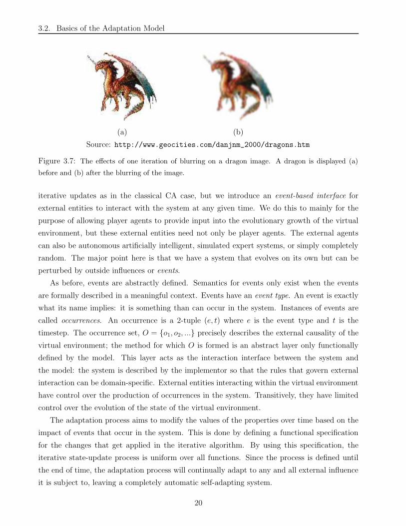
and a simultaneous update rule is applied: ∀x, y : px,y ← p′x,y. A good demonstration of the
locality of the effects of the blurring algorithm can be found in Figure 3.6. The larger-scale
effects of blurring an image are shown in Figure 3.7.
We extend this model to include a means for tweaking the state of the system externally.
That is to say that the system can evolve in and of itself by the continual application of
19
3.2. Basics of the Adaptation Model
(a) (b)
Source: http://www.geocities.com/danjnm_2000/dragons.htm
Figure 3.7: The effects of one iteration of blurring on a dragon image. A dragon is displayed (a)
before and (b) after the blurring of the image.
iterative updates as in the classical CA case, but we introduce an event-based interface for
external entities to interact with the system at any given time. We do this to mainly for the
purpose of allowing player agents to provide input into the evolutionary growth of the virtual
environment, but these external entities need not only be player agents. The external agents
can also be autonomous artificially intelligent, simulated expert systems, or simply completely
random. The major point here is that we have a system that evolves on its own but can be
perturbed by outside influences or events.
As before, events are abstractly defined. Semantics for events only exist when the events
are formally described in a meaningful context. Events have an event type. An event is exactly
what its name implies: it is something than can occur in the system. Instances of events are
called occurrences. An occurrence is a 2-tuple (e, t) where e is the event type and t is the
timestep. The occurrence set, O = {o1, o2, ...} precisely describes the external causality of the
virtual environment; the method for which O is formed is an abstract layer only functionally
defined by the model. This layer acts as the interaction interface between the system and
the model: the system is described by the implementor so that the rules that govern external
interaction can be domain-specific. External entities interacting within the virtual environment
have control over the production of occurrences in the system. Transitively, they have limited
control over the evolution of the state of the virtual environment.
The adaptation process aims to modify the values of the properties over time based on the
impact of events that occur in the system. This is done by defining a functional specification
for the changes that get applied in the iterative algorithm. By using this specification, the
iterative state-update process is uniform over all functions. Since the process is defined until
the end of time, the adaptation process will continually adapt to any and all external influence
it is subject to, leaving a completely automatic self-adapting system.
20

3.2. Basics of the Adaptation Model
EVENT SET
OCCURRENCE SETuser input
ADAPTATION t
INCREMENT
ENGINE
Figure 3.8: The causal block diagram representing the general adaptation process.
As a result of the abstractions, the model splits itself into an adaptation engine module which
is completely generic and the adaptation system sub-modules which are not at all generic. These
sub-modules plug into the adaptation engine and use it to modify the state of the adaptation
system. The implementor of the system modules is completely free to build a customized virtual
environment which adheres to the adaptation model, and use the adaptation engine to perform
the adaptive tasks required by the system.
The general idea is summarized by a causal block diagram [PdLV02] in Figure 3.8.
3.2.1 Generic Adaptation Procedures
Experimental evidence has shown that there are some generic adaptation concepts which are
common to most systems and thus can be more generically formulated. Such algorithms further
generalize the model and hence increase the overall usefulness of the framework. Most concepts
listed below are simply intuitive constructions obtained by reflecting upon the adaptation pro-
cess.
Simultaneous Cell-Update Masks
As stated in the previous section, the value of the properties on each cell change in time
as a function of the values on neighboring cells at the previous time step. It is natural for
programmers to implement the effects of the updates to cell values (at a given time in the
21

3.2. Basics of the Adaptation Model
0 0 0 000
0 0 000
0
20 2020 20
5 8 8 79 12 11 87 9 7 44 5 4 4
0 0 0 000
0 0 000
0
20 2020 20
5
5 5
577
7777
779 99 9
(a) (b)
Figure 3.9: A region affected by modifications after 1 timestep of blurring using (a) sequential iterative
updates and (b) simultaneous update rules
timeline) as a sequential iteration over all grid cells. This causes a bias problem, because for a
given cell-update, the value of its neighbors could already have been modified due to the order
of the iteration. The effect of the bias in an example of blurring is demonstrated in Figure 3.9a.
The modifications made to the cells assume no intermediate representations between time
steps: their values change simultaneously. The new value is strictly a function of current values.
There can also be any number of properties on a grid cell. To implement this, we propose using
cell-update masks, or simply masks.
Masks are temporary grids that hold only the modifications to be applied to the grid for
each grid cell. The adaptation algorithms calculate the modifications, store the modifications
temporarily in the corresponding section in the grid. When all the calculations are done for
the iteration, the mask is then applied to the grid: all modifications in each grid section in the
mask are applied to the corresponding grid section in the real grid. Then, the mask is cleared
for the next time step, and the process repeats at each time step.
Vector Averaging and Angular Propagation
As in blurring, grid properties in cellular automata are commonly scalar properties. SimCity
is an example of classic game that relies on cellular automata techniques [Sta96], associating
scalar quantities with grid cells. In SimCity each grid cell may have scalar properties such as
pollution levels, crime rates, land value, and so on. There is, however, no reason to restrict grid
properties to scalar values.
We define a discrete vector field as VG : G → <2, so that for each grid section g ∈ G,
there exists an associated vector. The vector at cell (3, 2) will be denoted ~g3,2. Note that a
2-dimensional vector can be thought of as a magnitude and angle; when we are interested in
just one component of the vector we can reduce it to the scalar case; e.g., a simple angle value
22

3.2. Basics of the Adaptation Model
Figure 3.10: Affect of an update on one grid section (assuming γ = 1), showing a) before the change
b) before the update on the middle grid section c) after the change and update
θ3,2.
Vector averaging is a technique analogous to image blurring, except on vector components
rather than scalar components. We initially ignore the vector’s magnitude and assume it does
not change. Each ~gi,j is then modified to have a new angle computed as a weighted average of
its own state and neighboring angles. Suppose we have an average angle θg for a grid section g
and its neighborhood. We define a shift from (~g′, ~g) for each neighbor g′ as the difference θg−θg′ .
In the special case where g′ = g′, the shift represents the discrepancy between an angle and
its relative neighborhood average. For simplicity, we assume that all angles have the smallest
possible magnitude and sign respect the unit circle convention. That is, −π ≤ θ ≤ +π,
θg = 0 points “east”, θg = −π point is “west”, θg = +π2
points “north”, and θg = −π2
points “south”. Note that we assume this for all angles, so that shift from (i,−j) = −π2, not
3π2
. If the result of any mathematical calculations gives an angle outside these bounds, the
angles are immediately cyclized (repetitive addition or subtraction of 2π) until they are within
these bounds. An immediate consequence of this construction is that given any two vectors,
shift from(~v1, ~v2) = cyclize(θ2 − θ1).
As in blurring, the values approach their current relative neighborhood average. The total
angular change for g is then some proportion of shift from g, for some constant γ, δg = γ ·
shift from(~g). The update rule then becomes: ∀g ∈ G : θg ← θg + δg, applied simultaneously
(using masks) over all grid sections.
To demonstrate the effects of vector averaging, consider a single grid section surrounded by
its 8-neighborhood [Tou], all of its vectors pointing eastward (θ = 0) with arbitrary magnitude,
as seen in Figure 3.10. Now, if we shift each surrounding vector by 90◦, the average will shift
by ∆θ = (8/9)∗90◦ = 80◦, so the update will shift the middle vector’s angle by δ = γ∆θ. Since
the middle vector has shifted, upon the next application of the update (the next iteration) it
will in turn cause a difference in average of all points for which it is a neighbor. This will cause
those grid sections’ vectors to update, and so on. As a result, a change in angle propagates
through the grid via its neighboring cells, but loses influence each iteration.
23

3.2. Basics of the Adaptation Model
The long-term effects of a sudden change in angles over time is called angular propagation.
The effects of the changes are transferred to the surrounding areas over time until the influence
of the change is negligible. By adjusting weight parameters such as γ local turbulence can be
damped according to the needs of the system being modeled. A high value for γ may signify a
region particularly sensitive to change, whereas a lower value indicates a resistance to change.
Angular propagation can be caused by occurrences of events. The propagation shown in this
section was an example of a specific type of propagation applied to changes in angles of vectors.
However, the propagation concept itself is more general. If after 3000 iterations of blurring a
sudden block of black pixels were added, the event would cause an impact that would propagate
the dark colors to spread around evenly over the image. The system is thus adapting to the
occurrence by propagating effects of event occurrences to its surroundings.
Flow-based Fuzzy Property Update Rules
Non-constant scalar properties on grid sections can be modified differently than simple aver-
aging. When blurring, values are modified and set directly to the value of a given calculation
involving local and neighboring values (the average). A flow instead describes the transfer of
information between neighboring grid sections. When using flows, properties values are treated
as quantities that are displaced from one grid cell to a neighboring grid cell. The flow function
for a given property or set of properties describes precisely how information is transferred from
one grid cell to the next.
Vectors on each grid section describe a strength and direction of flow. The flow function
computes how much of a property is transferred from a grid cell to the cells in its neighborhood
as a result of the value of the vector property. Therefore, a flow function takes a vector as a
parameter and returns a set of displacement maps of the form (g, g ′ : g[p]← g[p]−k ·g[p], g′[p]←
g′[p]+k ·g[p]) where g′ is a neighbor of g, k ·g[p] is the amount of the property p to be displaced
from g to g′, and 0 ≤ k ≤ 1. The adaptation process applies the flow changes described by the
displacement maps for each grid section at each iteration of the computation.
We use a fuzzy approach similar to fuzzy control to compute flow displacements for a more
natural flow dispersal. The flow function can be formulated as a fuzzy controller. Formally,
the flow function consists of n fuzzy components: z1, z2, · · · , zn. Here, zj is an arbitrary fuzzy
membership function zx(~g) ∈ [0, 1] which represents the raw influence of that component over
a given property. The influences of the components are analogous to the values of the actions
obtained by querying a fuzzy rule-base. The displacements returned by the flow functions are
analogous to the actions chosen by a fuzzy controller. Fuzzy control is still used to query a
rule-base and the outcomes measure the influence of the displacement actions. The rule-base
24

3.2. Basics of the Adaptation Model
is created by the designer of the example application system.
In this case we allow simultaneous actions to be chosen and performed. The result of
this difference is that several displacement maps are created, each with different values of the
proportion parameter, k. To obtain k, the membership values are normalized so that they
represent the local influence in comparison to other influences:
fx(~gi,j, pi,j) =zx(~gi,j, pi,j)
∑ny=1 zy(~gi,j, pi,j)
To make this more clear, consider a scenario where the components are associated with the
four major cardinal directions: zN , zE, zS, zW . The amount transfered in each direction is
proportional to the corresponding flow influence value fdir. At each iteration, ∆pW = kp ∗
fW (~gi,j, pi,j) ∗ pi,j is the amount of pi,j that is displaced westwards, where the proportion pa-
rameter 0 < kp <= 1 is the rate of transfer. The simultaneous update rules for this component
would then be: R1 : pi−1,j ← pi−1,j +∆pW and R2 : pi, ← pi,j−∆pW . Components for other di-
rections are treated similarly. Note that it is also possible to define hybrid components, formed
by the conjunction or disjunction of the fuzzy properties; e.g., zNW = zN AND zW . Then the
displacement of moisture would be listed as a rule set in a fuzzy controller system as is done
in [McC00].
The actual behavior of the flow depends on the membership functions used; if a system
demands a smooth flow, then naturally the membership functions should reflect that. The
role of the fuzzy membership functions are to shape the flow. If, for instance we use a “crisp”
function, one with a sharply-defined peak such as:
zN =
1 if π/2− ε <= θ <= π/2 + ε;
0 otherwise.(3.2)
for small ε, then the westward flow will move somewhat discretely. A smoother function like:
zN =4
π
√
(π
4)2 − (x−
π
2)2 (3.3)
will lead to a smoother spreading.
Several advantages are gained by formulating the flow function as a fuzzy controller. First,
it allows the designers of an application system to describe linguistic variables for flow com-
ponents. Linguistic variables quantify vagueness by construction and as such can be easier to
model when the exact information is not available. Secondly, the examples above use vectors
for flow components, but this is not generally necessary. Flow components can also be scalar
or other values, as long as a membership function can be defined from the arbitrary domain to
a value in [0, 1]. This fact allows designers to define complex arbitrary components that can
25

3.2. Basics of the Adaptation Model
still be made meaningful by way of a particular membership function. Thirdly, the rule base
is a widely familiar construct and often easy to use as well as easy to modify. Rule bases give
the application designer a natural modeling environment along with the flexibility of describing
flows based on logical statements that can involve many factors. Lastly, fuzzy controllers can
themselves be internally adaptive [Wan96], allowing the flow functions to change based on given
criteria.
In this chapter, the core concepts of the generic adaptation model were introduced. The
abstract model is simply a grid that is separated into grid cells paired with an adaptation
process that modifies the values of grid cell properties automatically over time. The properties
are global but can have different local values on individual grid sections. Adaptation is a
process that changes the local properties values automatically over time. Local adaptation
is adaptation which uses the values of neighboring cells to influence the modification of grid
cell property values. External entities are allowed to interact with the adaptive system by
causing occurrences of specified events. The adaptation process reacts to these occurrences by
applying abstract adaptation procedures at each iteration. Examples of external entities could
be players, or artificially intelligent bots.
The adaptation procedures are defined by the specific application of the model. The pro-
cedures defined by the applications are algorithmic modifications of the generic properties.
Semantics for abstractly defined properties and adaptation procedures are given by the de-
scription of the application system. The application systems are therefore thin instances of
the generic model. Examples of such application systems will described and analyzed in the
following chapter.
26

Chapter 4
Applications of the Model
In this chapter, we show specific applications of the generic abstract model. The aim of these
applications is to emulate real-world systems. For this reason, we also call these applications
example systems. Since these systems are built in the adaptation model presented in Chapter 3,
they are inherently locally-adaptive. The applications in fact define semantics of a context by
giving meanings to property values and providing specific procedures that describe the evolution
of the data values over time. Additionally, each application specifically describes the events
that can occur in the system and the entities that can cause them. In the end, an example
system describes an adaptive virtual environment (AVE) which game players can explore.
In designing example virtual environments for systems to apply the adaptation model to, we
noticed that systems we had created can be classified into 2 top-level categories: environment-
based applications, and agent-based applications. Both types of applications adapt based on a
set of criteria; the difference is how the criteria is obtained. Environment-based applications
are adaptation systems that adapt depending entirely on values in the environment itself.
Agent-based applications adapt depending on the observations of agent behavior data as well
as environmental factors. Agents here take on their usual definition: they are simply entities
that interact with the system (or with each other) in some way.
Each section describes one or more applications of the model. Initially, the system is de-
scribed in general; and the criteria for adaptation in these systems are discussed. Then, the
system is formalized conceptually by breaking it down into its major algorithmic components.
Adaptation algorithms operate on meaningful data which are mapped to property values in
the model. The components are then fit into adaptation procedures, each of which calculates
the changes to values due to local adaptation. The adaptation process applies these changes
at each iteration of the overall process. We also suggest events that may occur in each sys-
tem along with their effects on the system and analyze the behaviors of the systems using the
27

4.1. Environment-based Applications
implementation described in Chapter 6.
4.1 Environment-based Applications
Environment-based applications are adaptive systems that change over time based on the values
of the surrounding environmental properties. Examples of environmental properties will be
given in the specific system being described.
Typically in modern games, the only role played by the environment is to provide a virtual
setting for the players to play in. The setting has a certain effect on the immersion and the
experience felt by the players, but is usually purely aesthetic rather than responsive. The only
interaction players have with the environment is with other players or other agents (monsters,
etc.). The players can discover the world in time, but they can never really change it, not even
indirectly. The environment can change due to game progression, but just in a predefined way.
Environment-based adaptation is an automatic means for the environment to adapt to itself;
for example, a tree growing around a physical barrier (power lines) instead of through it, the
water level of the sea rising as a consequence of lunar positioning, natural selection. These are
all examples of environment-based adaptation.
These examples all contain objects, entities, or things the players should be able to interact
with. By expanding the interactive capabilities of the entities and the environment, players
could affect the state of the system more meaningfully than by simply gaining more levels and
more equipment. In certain cases, allowing the players to interact with the environment, even in
very simple ways, should in turn lead to some adaptive behavior, ie. a long-term reaction from
the environment. For example, in a medieval fantasy setting, a powerful player sorcerer could
cast a spell to remove the natural production of water in a given region. An environment-based
application would react to this: after some time the ecosystem would die or deteriorate unless
it found another source of water.
4.1.1 An Adaptive Weather System
In computer games, weather simulation is commonly implemented to contribute to a pseudo-
realistic world. It is common because it is easy to implement as a randomized system and adds
realism. A physical world without any weather would soon become unbelievable. The overall
end result is that the players’ game experience is improved, most players are satisfied with a
random weather simulation system because to them it appears like a possible real system. When
one cannot make the computerized system behave exactly like a real-world system, making parts
28

4.1. Environment-based Applications
of the world at least appear real is a general goal in computer games.
The goals of this research are similar. In particular, we focus more on improving the
appearance of the system rather than making it more realistic. That is, we search for an
adaptation process that emulates real-world adaptation.
Weather simulation is typically considered a computationally intensive application, largely
reserved for supercomputers. In the virtual worlds of computer games, however, physical accu-
racy is less critical, and much simpler approaches suffice to produce aesthetic, in-game climate
effects. Note that by proposing to add adaptation to a non-adaptive simulation system we are
proposing to make it more like the real system it is modeling. As such, we are also indirectly
and inevitably making the system more realistic. However, this is not our intention; it is a
coincidental consequence.
Weather System Description
In its simplest form, a weather cycle displaces moisture: water from lakes and seas is carried by
wind to cooler locations, where the reduced water capacity of cooler air causes condensation;
rain water eventually runs downhill to refill lakes and oceans [Ent04]. There are several factors
that can affect this process, including altitude and terrain structure, wind, temperature, and
so on. Each of these can be quantified as a value-based property in our system. The value of
the property indicates the significance of the factor in the AVE.
We have modeled our weather system upon the following basic precepts:
1. Wind gathers moisture from bodies of water, and loses water at higher altitudes.
2. Water flows downstream.
3. Altitude affects wind patterns.
These basic precepts will be transformed into adaptation procedures (update rules) following
the process outlined in Section 3.2. We must however first properly define the data in the
adaptive weather system.
There are 2 basic scalar data values suggested by the basic precepts listed above: moisture
and altitude. Moisture represents the density of water in the air. Swamps, bodies of water,
humid regions have high moisture, whereas dry places like deserts have low moisture. Altitude
is the height of the ground relative to sea level. High regions like hills or mountains have high
altitude whereas lower regions like valleys and oceans have low values. The geographic location
usually influences a region’s climate because each physical location has a different configuration
of their surrounding environmental properties.
29

4.1. Environment-based Applications
50
9085
75
601020
40
30
Figure 4.1: Example gradient vector representation. Grid cells show local terrain altitudes.
The scalar values were limited to being between two chosen extremes: glow = −5000 and
ghigh = 5000. It can never be the case that a value is higher than the high extreme or lower
than the low extreme. In this system, the physical correspondence is that there are saturation
thresholds for moisture and dryness. A good example is that an ocean or sea cannot get any
more moist: they are at ghigh.
There is 1 basic vector value: the wind. The magnitude of the vector describes the strength
of the wind and its direction describes the direction of the wind. There is one more vector
property which is an induced property called the gradient vector. The gradient vector on a
grid section points to the direction of descent, and its magnitude represents the steepness of
the grade. Due to gravity, moisture flows downstream in the direction of the gradient and is
described as a a fuzzy flow controller (see Section 3.2.1).
The gradient is a vector sum composed of vector components whose magnitudes are differ-
ences in altitude values of surrounding cells. The magnitudes of the vectors are determined
by subtracting the terrain altitude from the altitude of a neighboring cell, with corners of the
8-neighborhood having a weight factor or√
22
. The direction of each vector in the sum is given
by the position of the neighbor relative to the center. Figure 4.1 shows an example gradient
induced from the altitude values of its surroundings. If we assume unit vectors for each of the
cardinal directions and therefore the identities N = −S and W = −E, then the calculation
looks like:
~vgrad = (50− 10)N + ((50− 60)sin(π
2)N + (50− 60)cos(
π
2)E)
+(50− 75)E + ((50− 90)sin(π
2)S + (50− 90)cos(
π
2)E)
+(50− 85)S + ((50− 40)sin(π
2)S + (50− 40)cos(
π
2)W )
+(50− 30)W + ((50− 20)sin(π
2)N + (50− 20)cos(
π
2)W )
= 54.142N − 60.35534E − 56.2132S + 48.28427W
30

4.1. Environment-based Applications
50
5050
50
30 30
30
50 30
(a) (b)
Figure 4.2: Example of degenerate cases where (a) ~vgrad = 0 and (b) ~vwind avg = 0.
= 108.64W + 110.35N
giving a vector with angle tan−1(110.35/108.64) = 45.45◦ north of west.
The inverse gradient points in the direction of ascent, and is used to determine how wind
direction is altered by the current terrain. If a gust of wind is pointing into a wall, it will
instead blow around it. For wind to move around higher-altitude obstacles it must therefore
be pushed away from the direction of the inverse gradient or, equivalently in 2D, towards the
direction of the gradient.
Another induced property is the current local average wind value. The average wind value
is a vector whose magnitude is equal to the sum of all wind magnitudes in the 9-region divided
by 9; the average direction is precisely the direction obtained by the sum of all the vectors.
Comparing the current wind value with the current average gives a summary of how the current
wind value on a cell differs from its immediate surroundings.
Note that degenerate data representations are possible, as shown in Figure 4.2. For instance,
it is possible that the gradient has a 0 magnitude even though not all of the neighbor values are
equal to the current cell value. As well, the current average could have no direction at all when
all the vectors sum to a vector whose component magnitudes are all 0, or worse: numerical error
could lead to an arbitrary angle. These are of course due to the fact that what is described
here are approximations. In practice, we should be aware of these limitations and deal with
them accordingly.
Weather Adaptation Procedures
There are 3 major adaptation procedures in the weather system: moisturewind, gradDev, and
rain. The procedures are functional algorithms that perform the actions needed for adaptation
such as checking the values of some criteria and modifying values as a consequence. In this
subsection, we will thoroughly explain the steps in each procedure.
31

4.1. Environment-based Applications
TARGETvGRADv
vWIND_AVG
Figure 4.3: An example of obtaining ~vtarget given ~vgrad, ~vwind avg , and α = 0.8
The gradDev procedure represents the bending of the wind vectors over time due to the
values of altitude. The procedure uses the vector averaging and angular propagation concept
explained in Section 3.2.1. The current wind vector is shifted towards some target vector,
denoted ~vtarget. The shift is scaled by some damping parameter, 0 < γ < 1, which roughly
corresponds to the speed of the shift since one shift is applied per iteration of the adaptation
process. For example, when γ = 0.1 it would theoretically take 10 shifts before ~vwind = ~vtarget,
as opposed to 100 shifts if γ = 0.01, assuming of course no perturbation from other factors such
as angular propagation. Note that the damping parameter γ is similar to the weight parameter
used in Reinforcement Learning [SB98] update rules. The damping parameter is chosen by the
modeler depending on the specific needs of the system.
As previously mentioned, the most influential contributing factor to the wind shifting is the
gradient vector. We also incorporate an inertial factor, to give a smoother flow pattern; we
designate ~vtarget as some composition of the gradient vector and current average wind vector.
The composition is such that θtarget = θwind avg + α · shift from(~vwind avg, ~vgrad). An illustration
of obtaining ~vtarget is found in Figure 4.3. Again, α is a damping parameter which affects
the smoothness of the transitions versus the angular propagation due to influence from the
surroundings. This parameter further increases the flexibility available to the users of the
application.
Moisture is displaced in two ways: by the rain procedure and by the moisturewind pro-
cedure. Both procedures use fuzzy flow-update rules to transfer scalar values between neigh-
bors. Similarly to the gradDev procedure, each flow-update rule has a damping parameter
(kmoisturewind and krain) associated with them which scales the actual modification allowing the
modeler to easily modify the influence of the moisture-altering procedures.
In the moisturewind procedure, four independent components that comprise the wind are
represented by the cardinal directions: ~vN , ~vE, ~vS, ~vW . The value of each component is calculated
32
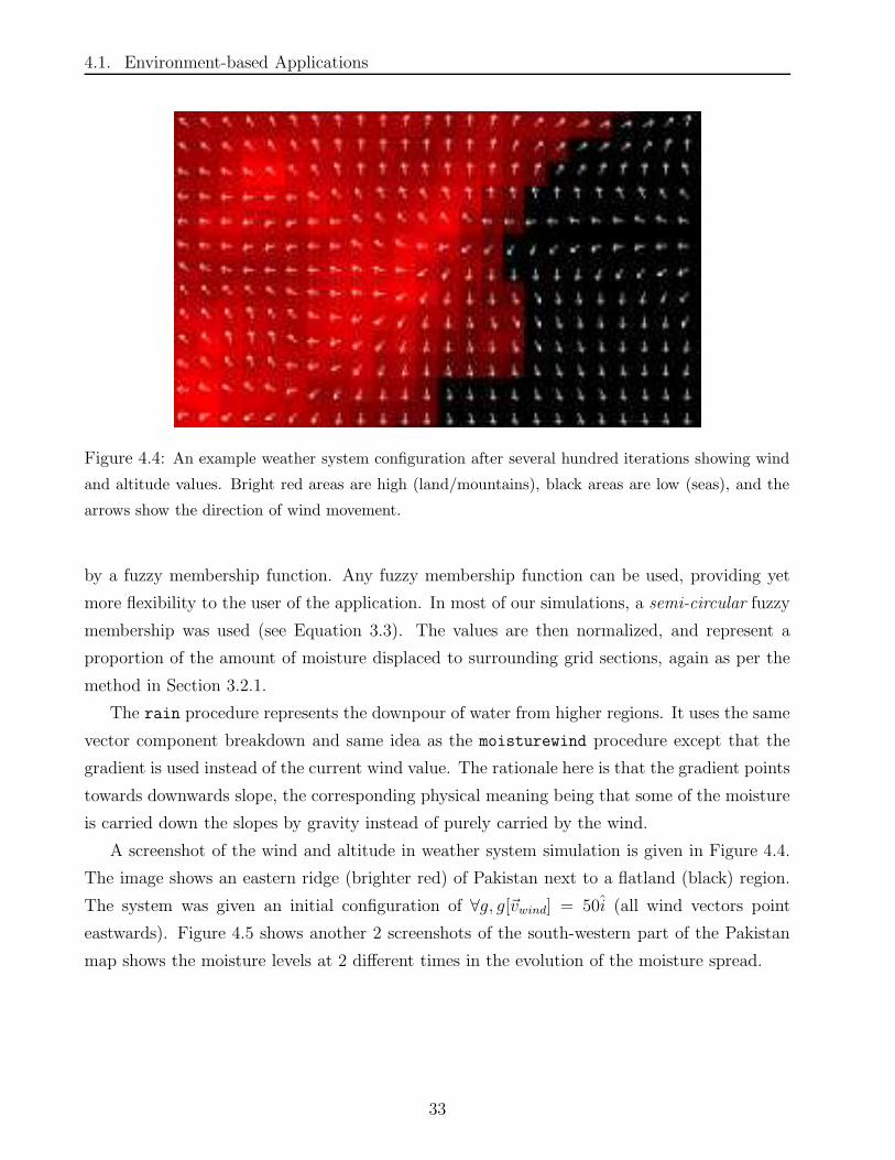
4.1. Environment-based Applications
Figure 4.4: An example weather system configuration after several hundred iterations showing wind
and altitude values. Bright red areas are high (land/mountains), black areas are low (seas), and the
arrows show the direction of wind movement.
by a fuzzy membership function. Any fuzzy membership function can be used, providing yet
more flexibility to the user of the application. In most of our simulations, a semi-circular fuzzy
membership was used (see Equation 3.3). The values are then normalized, and represent a
proportion of the amount of moisture displaced to surrounding grid sections, again as per the
method in Section 3.2.1.
The rain procedure represents the downpour of water from higher regions. It uses the same
vector component breakdown and same idea as the moisturewind procedure except that the
gradient is used instead of the current wind value. The rationale here is that the gradient points
towards downwards slope, the corresponding physical meaning being that some of the moisture
is carried down the slopes by gravity instead of purely carried by the wind.
A screenshot of the wind and altitude in weather system simulation is given in Figure 4.4.
The image shows an eastern ridge (brighter red) of Pakistan next to a flatland (black) region.
The system was given an initial configuration of ∀g, g[~vwind] = 50i (all wind vectors point
eastwards). Figure 4.5 shows another 2 screenshots of the south-western part of the Pakistan
map shows the moisture levels at 2 different times in the evolution of the moisture spread.
33

4.1. Environment-based Applications
(a) (b)
Figure 4.5: An example weather system configuration after (a) 100 iterations and (b) 300 iterations
showing moisture values and wind vectors. Bright green areas signify high moisture regions whereas
darker region correspond to dry regions.
Terrain Generation
Automatic terrain generation is often desired for computer games. Since terrain influences
weather and represents a crucial part of any real-world natural environment, it seems to fit
intuitively into a weather system.
Two methods were investigated for terrain (altitude) generation. The first method includes
3 steps: a coarse random distribution, a smoothing pass, and rescaling. The first step was a
simple iteration over every grid section that assigned some uniformly random value between
glow and ghigh to the altitude property on that grid section. The resulting altitude maps are
too coarse to be realistic, so they are blurred a number of times to smooth the surface. The
smoothing also removes many of the sharper parts of the altitude map. To accommodate,
the minimum and maximum values over the entire grid are found, and then then for each grid
section the value of altitude is scaled proportionally to [glow, ghigh]. As a result, there contains at
least one value (the maximum value) that is equal to ghigh and at least one value (the minimum
value) that is equal to glow. The advantage of this first method is that it is easy to implement,
simple to understand, and rather efficient. However, the disadvantage is that it provides a less
realistic result which may be extremal in local variation.
The second method used real-world physical location data obtained by the DIVA-GIS project
34

4.1. Environment-based Applications
[RHG03]. The DIVA-GIS information archive contained sufficiently accurate altitude maps of
many locations across the world. The problem for this particular application was that the
maps were actually too detailed to be easily represented during prototyping. Therefore, a re-
sampling process was run to downscale the data: the points were organized into 2x2 square
regions containing 4 points each, the values of the 4 altitude points are averaged and then
considered 1 point in the new map. In the case of odd-number points on one of the axes,
the last row or column of sections becomes 3x2, 2x3 or 3x3. This special case creates a loss-
of-information bias towards the outer points, but since the loss is minimal the bias is not a
critical issue. Since the boundary of these maps is arbitrary, we could have also simply omit
the outermost points altogether. We chose to include them as to encourage the least amount
of information loss. The re-sampling is repeated until the map is sufficiently small enough to
represent on a screen. Some larger samples were also kept for performance measurements to be
taken (see Section 6.3).
Boundary Conditions
Carefully-designed boundary conditions are important for many systems to behave properly.
One common mistake in system design is to simply omit dealing with boundary cases. Such
errors often eventually lead to erratic observed behavior.
Two different boundary schemes for grids were examined. The first scheme was strictly-
bounded: the grid simply “ends” at the boundary points. In this scheme, the assumption is
made that there is nothing beyond the last grid section on a grid. The east-most grid sections
have no eastern neighbors. Similarly for all extreme sections and directions possible in grid
layout. Consequently, the extreme points had fewer neighbors which causes some bias in the
calculations containing local property values. The effects of this bias on the random method of
terrain generation can be seen in in Figure 4.7: as a result of generating a random terrain, the
outer ridges have lower altitude than the rest of the grid.
The other boundary scheme is to have no boundaries at all. The east neighbor of the
eastern-most point on the grid is the western-most point in the same row. Similarly for west-
ern neighbors of western extremities, and for the north/south axis as well. This boundary
scheme corresponds to the torus mathematical topology. This scheme also removes the bias
on the edges. By default unless otherwise mentioned, this boundary condition was used in all
simulations.
35

4.1. Environment-based Applications
Figure 4.6: An example tornado.
Weather Events
Incorporating interesting weather events is also possible and likely desirable. Events can be
anything that affects the properties in the system such as earthquakes, tornadoes, tsunamis,
storms, etc..
We have modeled “tornadoes” as local, non-linear dynamical systems with the stable fixed
points at their centers. A 2-dimensional dynamical system [Str01] represents the wind flow
within a specified sub-grid such that the center point is fixed point in a stable spiral. Within
this sub-grid, the wind vectors are no longer influenced at all by outward sources; they are
only part of the tornado. The outer vectors are treated normally. As a result, the effect of the
tornado’s turbulence is spread with decreasing influence out to the surrounding grid sections
via angular propagation.
The tornado moves by slightly displacing the sub-grid (along with it, the fixed point) at
each iteration and reassigning the values in the sub-grid dynamical system around it. The
movement of the tornado is defined by some arbitrary function of timesteps and could be
randomly generated in the same way that path models are generated for mobile agents (see
Section 6.2). Figure 4.6 shows a screenshot of a tornado on a flat terrain. We will measure the
efficiency of the implementation of tornadoes in Section 6.3.
36

4.1. Environment-based Applications
Figure 4.7: An example hexagonal grid in the weather system.
Hexagonal Grid Representation
As stated in Section 3.2, since the adaptation process is based entirely on neighbors in some
metric space the theory extends to metric spaces other than a rectangular grid. A hexagonal
grid is a “nice” metric space because notion of neighborhood is particularly intuitive. Two cells
are neighbors in a hexagonal grid if they share an edge, or equivalently, if the distance between
them is 1. A neighborhood of a cell in the hexagonal grid is its 6 immediate neighbors.
The adaptation process here remains unchanged. The neighboring cells are equally distant
from a given cell, so the gradient calculation becomes even simpler because there are no special
case “corner-neighbors”. Six fuzzy actions instead of 4 need to be defined for the flow controllers
in the moisture spread procedures, but otherwise flow updates remain the same.
A capture of the hexagonal grid weather system is displayed in Figure 4.7.
Analysis of Weather System Behavior
All the major components of the weather system have now been described. The question still
remains: how does this system behave? The answer to this question is presented in detail here.
An important concern is the performance of the adaptive system; it must of course be at
least efficient enough to be usable. We will defer performance analysis until we describe the
37

4.1. Environment-based Applications
implementation in more detail, in Chapter 6. Another important concern is how well it achieves
its purpose: does it act in a stable, aesthetically appealing manner or does it produce completely
random and/or meaningless weather effects.
Moisture dispersal seems to happen as smoothly as expected. Areas of pure saturation
develop in the flatter regions, bits of moisture are carried around the edges of these areas and
in particularly windy areas. Playing with the values of the damping constants for the effect of
wind vs. rain produces the expected resulting behavior, which is reassuring.
As mentioned in the description of the gradDev procedure, there are several factors that
affect the wind’s change. A concern, then, is whether the combination of these influences
leads to the wind changing forever or does it instead approach convergence to a fixed state. If
the wind vector moves towards the gradient every iteration, it is certainly going to converge
eventually. However, the average wind vector might not necessarily remain the same and, in
particular, might move away from the gradient. In cases where the average wind moves away
from the gradient, ~vtarget also moves away from the gradient. As a result, the direction of wind
change will depend on which side of ~vtarget the wind vector is on, which depends on α.
If α = 1, then ~vtarget = ~vgrad so no matter how deviant the wind average is, the wind vector
will always approach ~vgrad and so is certain to converge. In contrast, if α = 0, the wind will
always approach the average. In our chosen starting state, this immediately converges as well
since the average wind vector for every grid cell is 509i. What about convergence conditions
when 0 < α < 1 ? A closed-form expression for convergence conditions would be useful to have.
Assuming we ignore magnitude, in general the wind vector, ~vij,wind, on a given grid section
gij will undergo the following update at each iteration:
θij,wind ← θij,wind + γ · shift from(~vij,wind, ~vij,target)
= θij,wind + γ · cyclize(θij,target − θij,wind)
= θij,wind + γ · cyclize(θij,wind avg + α · cyclize(θij,grad − θij,wind avg)− θij,wind)
At first, the update rule looks like it takes the form of a one-dimensional iterated map [Str01]
Iterated maps are discrete-time dynamical systems in which a value xi+1 = f(xi) where i is an
iteration number. Research has been done on these systems; well-known techniques exist for
analyzing them. Unfortunately for us, not only do we actually have a set of these equations,
the function f is dependent on many of the set’s previous iteration values not just its own
previous value. If it were only for the former, then we could simply treat the wind-bending as a
collection of independent iterated maps and solve a general equation which would apply to all
of maps. The set of iterated values is {∀i, j|θij,wind} and θij,wind avg is actually a function of the
38

4.1. Environment-based Applications
Figure 4.8: ∆mask as a function of the timestep in a simulation run on the Pakistan terrain map.
neighborhood property values τ(gij[wind]). Therefore we have a (height · width)-dimensional
iterated map with equations of the form θij,wind = f(θi−1,j−1,wind, ..., θi+1,j+1,wind). This is a
complex system and hence it is difficult to solve analytically. It is also the case that components
of an adaptation system may be arbitrarily complex, and so proving convergence in general will
be difficult. Direct, practical techniques are more convincing.
We choose a quantitative approach to measure the convergence and effects of the damp-
ing parameters on the system’s behavior. In doing so, we define the overall change in wind-
deviations from one timestep to the next as the sum of a change in angles over all grid section.
Formally, this sum is:
∆mask =∑
i,j
|θtij,wind − θt−1
ij,wind|
At a fixed point, the wind vectors don’t change at all so this sum will continually be equal to
0. Note that ∆mask is expressed in radians.
An experiment was conducted to measure the values of ∆mask over time, assuming default
values of α = 0.2 and γ = 0.1. The maps of Pakistan, North Korea, and a randomly generated
terrain were used, each of which had both heights and widths of at least 50 grid cells. Every
experiment converged to ∆mask < 1 in less than 3000 iterations and convergence graphs look
similar. Figure 4.8 shows the precise values as a function of timestep using the Pakistan map.
The experiment included dynamically adding altitude values at certain times, which will be
explained below.
In general, the function is not non-decreasing: there are iterations where the ∆mask actually
increases. Increases are usually small (< 1) but not always negligible which implies that it
is not necessarily only caused by numerical error. However, on all 3 tests, the ∆mask did
indeed converge to essentially 0 (≈ 10−13) after 7000-8000 iterations and remained at this value
39

4.1. Environment-based Applications
endlessly. In fact, the converged value never reached exactly 0 due to some minimum amount
of numerical error.
As mentioned above, patches of altitude were added to the map dynamically during its
evolution. The reason for this functionality is to see how the system reacts to sudden changes
once it has stabilized. A small patch of approximately 10-15 altitudes of ghigh were added at
t ≈ 1500 and a larger patch (20-30 altitudes of ghigh) at t ≈ 3000. Both patches of altitude
were added to completely flat areas. The system reacted to these “sudden growths” by slowly
bending the wind vectors around them, and returned to a stable/fixed state within at most
100-150 timesteps, as show in Figure 4.8.
The tests above assume specific values of α and γ. We have shown convergence and stable
behavior in a particular case. Above, it was implied that convergence is somewhat dependent
on the values of these damping parameters. Looking back at the equation for the update of
θij,wind we see that γ is just a proportion of the shift towards ~vtarget. So as long as γ > 0 then
convergence only depends on α. Therefore, simulations were run on the Pakistan map with
γ = 1 and α = {0.0, 0.05, 0.1, 0.15, ..., 0.95, 1.0}. The results of the simulations are displayed
in Figure 4.9. Note that not all values are present. Each simulation was stopped at 10000
iterations if it had not yet converged. Many had not converged.
The simulation runs for varying alpha values lead to a discovery of cyclic behavior in certain
cases. The corresponding representation in the convergence graph is a long stretch of non-
continuous periodic values. In every case, the cycles started at some point before the 10000th
timestep and continued well beyond that point. As well, the cycles only formed when ∆mask < 5,
meaning the system had almost converged but entered a cycle instead of continuing. Re-running
the tests using a graphical interface showed that in all cases, a cycle corresponded to 2-6
neighboring wind vectors alternately “flipping” from one orientation to the another and then
back, while the rest of the map remained fixed. Detecting these cycles is non-trivial but not
difficult, however it does add an extra consideration to remember when using the application.
Values between 0.1 and 0.6 do not converge, while α > 0.7 seem to take longer to converge.
This isn’t necessarily a critical issue since the cycles only occur at low levels of ∆mask. One
could simply stop adapting once a threshold point of ∆mask ≤ 1 is reached. The specific cause
of this strange behavior remains unknown.
The last interesting addition to the system was control points. It is possible that one may
want some of the wind vectors to be entirely immune to change; for instance, as a way of
ensuring boundary conditions. This was enabled both statically and dynamically, and was
tested on several maps. The results were as expected: the control points allow the modeler to
force certain shapes of flow by using control points.
40

4.2. Agent-based Applications
Figure 4.9: Maximum timestep until convergence as a function of α after many simulation runs on
the Pakistan terrain map.
4.2 Agent-based Applications
Agent-based applications differ fundamentally from environment-based applications in that
agents contribute directly to the adaptation process. In environment-based adaptation, an ap-
plication designer could define agents in the AVE to interact with its surroundings and somehow
allow them to modify an environmental value. However, the adaptation process still only adapts
to the actual changes in the environment. In agent-based adaptation, properties of the actual
agents themselves are used to influence the adaptation process. That is, the adaptation process
observes the agents and their actions in addition to the rest of the environment. The focus of
the process is on the behavior of the agents, but uses environmental properties as well. Note
that this model presumes only localized information propagation but global effects could be
easily incorporated.
As briefly mentioned earlier, agents are simply entities that can interact with the environ-
ment or other agents. This definition is generic enough to allow agents of all kinds, and indeed
the flexibility is desired. Player agents are agents that are controlled by players of the game.
Player agents are usually called characters. Non-player agents come in many forms: monsters
(“mobs”), player companions (“pets”), non-player characters (”NPCs”) which can be guards,
41

4.2. Agent-based Applications
merchants, mercenaries, enemies, peasants, etc.. Agents need not be restricted to living crea-
tures but commonly are in MMOGs. In typical (static) virtual environments, the agents are
the only dynamic aspects of the environment. Here, both the environment and the agents are
dynamic and capable of influencing each other.
4.2.1 An Adaptive Reputation System
A player character’s in-game reputation is often an important component of the game environ-
ment, particularly for persistent-state games in which the same character is re-used for long
periods of time. Player actions that harm or help non-player agents agents should result in
a logically consistent reaction to the player, giving a greater sense of reality to the game en-
vironment. This is necessarily a dynamic property: player reputations need to be constantly
updated, and should also ameliorate over time and distance.
In order to allow reputation to more realistically disperse, a word-of-mouth model is em-
ployed to flow the impact of events caused by the agents. A game character’s reputation is
built by the spread of hearsay amongst the populace; reputation flow vectors modeling the
communication patterns of the general populace in each grid section are used to describe the
direction in which word of a positive or negative action will spread.
For our example system we developed a virtual communication terrain which, as in the
weather example, is represented as a discrete vector field. The difference is that the vectors on
this vector field do not change with respect to a static value such as the gradient. These vectors
are influenced solely by the agents’ velocity vectors currently occupying the corresponding grid
cell and some of its surroundings as well. The same wind model used in the weather system
then traces out the flow of reputation information.
In our case we simulated route popularity by tracking movements of semi-randomized agents
moving between cities following smooth curved paths, choosing destinations probabilistically
based on distance and city size to discover trade routes. The basic movement model for sim-
ulations is described below. In Chapter 5, movement models for agents are examined in much
greater detail.
Reputation events are abstractly defined even in this application: they are events that all
agents can cause that can potentially modify their reputation. They are only slightly analogous
to the weather system events because in these cases, the players are free to generate occurrences
as well as computer-controlled entities. Rescuing the princess, killing a commoner, stealing from
tavern, etc.. These are all examples of reputation events.
Positive and negative reputation points (RPs) are created on a grid section when a reputation
42

4.2. Agent-based Applications
event occurs at that location. The amount of RPs is proportional to the severity of the event.
These points are displaced via the flow, and also dissipate at a slow rate. For each point that
dissipates on a grid section, the reputation of the player is altered at that location. This process
repeats until all the reputation points have dissipated, causing a local alteration in the player
character’s reputation. RP is one of the scalar grid properties.
The player character’s reputation value is another example of a scalar grid property. Whereas
the reputation points dissipate over time, they slowly modify the reputation value. Positive
reputation points will modify the reputation value to a higher value, representing an increase
in good reputation. Negative reputation points lower the reputation values.
Reputation Adaptation Procedures
The adaptation process in the weather system includes one cycle that iterates over all the grid
sections performing update calculations. In contrast, the adaptation process for the reputation
system is split into 2 parts: the agent update cycle, and the grid update cycle. The grid update
cycle is analogous to the weather system’s update cycle in that it performs calculations as an
iteration over all the grid sections. The agent cycle performs the agent-based update calculations
and their movement/interactivity simulation. Therefore, the reputation adaptation procedures
are split into two categories based on which update cycle they are contained in.
There are 3 main adaptation procedures: repEvent and agentBend, which are part of the
agents cycle and repwind, which is part of the grid cycle. The repEvent procedure generates
reputation events probabilistically depending on a few parameters. In the simulations, it is
assumed that agents provoke reputation events and so the reputation events only occur at the
current location of an agent. For each agent, that agent generates an event with a probability
of Pevent. If an event is generated by an agent, it is a good event with probability Pgood or
negative otherwise. A generated event has a severity proportional to its reputation points,
which is uniformly randomly generated between glow = −5000 and ghigh = +5000. When an
event is generated by an agent, the reputation points are deposited on the grid section the agent
is currently occupying.
The agentBend procedure modifies the values of the reputation flow vectors given the orien-
tation of the agents. In essence, an “aura” of vector influence is created by each of the agents.
The aura for a single agent is a small sub-grid surrounding the agent (centered on the agent) of
vectors. Each of the vectors have the same direction of the agent’s velocity and have magnitude
linearly inversely proportional to the Manhattan distance (in grid sections) away from the cen-
ter grid section, to a maximum of 3 grid sections away from the center. The idea is illustrated
in Figure 4.10. The resulting reputation flow vector for a grid section is the vector sum of all
43

4.2. Agent-based Applications
Figure 4.10: The aura of reputation flow vector influence created by one agent
the vectors induced by all the agents’ auras on that grid section. The reputation flow vectors
for all grid sections describe the flow of communication via agents throughout the grid.
The repEvent procedure spreads the reputation points using fuzzy flow-updates exactly
like moisture was spread by the wind in the weather system. The vectors in this case are
the reputation flow vectors. Here, however, reputation points are temporary. This procedure
also converts a number of reputation points to reputation value. Since this procedure is exe-
cuted repetitively, the reputation points will either be carried by the reputation flow vectors to
neighboring cells or converted to reputation values. When converted to reputation values, the
converted values are added to the reputation value on the current grid section.
The reputation value on a grid section corresponds to the value of a given player character’s
reputation at that location. Initially, the reputation is equal to gmid =glow+ghigh
2= 0, neutral.
The reputation value added (or subtracted, in the case of negative reputation points) to the grid
section converted from reputation points pertains to the player who caused the event. In our
simulations, there is only one player and the events are generated at random locations decided
by the paths of agents. The system is extended to groups of players in a following subsection.
A Movement Model for Mobile Agents
Despite the vastness of virtual environments in recent MMOGs, within them there seems to
exist a finite set of interest points placed by the game designers for the players to discover
and interact with. Examples of such interest points in existing games are: cities, settlements,
44

4.2. Agent-based Applications
borders, spawn points, cavern entrances, trade/merchant stations, meeting points, etc.. Non-
player agents often have reasons to visit these interest points as well as player agents. Over
time, these interest points become basins of player activity in the VE. It is clear that throughout
the course of game-playing, players do two things:
1. travel to and from interest points
2. remain at interest points for some period of time (presumably doing something interesting)
Our simple movement model is composed of 4 major components: the graph which dictates
which interest points are connected to (reachable by) which interest points, which interest point
is chosen to be the next agent’s destination, the shape of the path taken by the agent to reach
its destination, and how long the agent remains at the interest points. The simple version that
we present in this Chapter is completely random based on a few common sense assumptions.
More complex models for agent movement are investigated in Chapter 5.
Each interest point has a coordinate position in the continuous space which the grid is
approximating. The graph connecting some of the vertices is then a proximity graph [Tou91]:
the length of the edges correspond directly to distances between vertices (interest points).
Agents can only travel to an interest point sdest from ssource if the edge (ssource, sdest) is in the
edge set of the graph.
Interest points have a scalar significance, or size. The higher the value of the significance, the
more interesting this point is to visit. It is assumed as well that agents generally prefer shorter
distances than long ones, more so than how interesting a place is to visit. Therefore, when an
agent chooses a new destination, each neighbor of the current interest point is assigned a weight
value wneighbor = size/distance2. The neighbor is then chosen at random with a probability
proportional to its weight.
Agent paths are assumed to be slightly non-linear. A path model is derived from a contin-
uous function f(t) defined over t ∈ [0, 1] with the constraint that f(0) = f(1) = 0. The values
of this function at 0 ≤ t ≤ 1 are considered points on a 2D plane with Cartesian coordinates
(t, f(t)) and are then transformed to the path’s coordinates by using basic affine transforma-
tion methods [FvDFH95]. The transformation defines a parametric curve on the continuous
space with f(0) representing the starting interest point and f(1) representing the end-point.
The transformation is represented by Figure 6.3. Basic non-linear functions were used such as
sinusoids, quadratics, cubics, quadrics, conics, and compositions of these as well. To generate
a path, a random model was chosen along with random parameters (eg. amplitude) and the
agent followed the path outlined by the curve f([0, 1]).
45

4.2. Agent-based Applications
Finally, the time between interest points was not explicitly modeled. At each iteration of
the adaptation process, with a probability Pagent newdest a random agent was chosen among
the agents to choose a new destination. Once the agent reaches the destination, it “hovers”
around the destination choosing random straight paths and turning to remain within a given
radius of the interest point. When not following a path, the agents use a typical velocity-based
Newtonian physical model for movement. Shifts in direction and velocity are probabilistically
determined.
Faction versus Reputation
Faction is a system similar to reputation that is currently used in a number of modern persistent-
state games, notably EverQuest. Faction is a system that measures relationships between
individuals and/or groups and is at times misunderstood to be the equivalent of reputation
[Bro03]. The terminology used is as follows: “an individual’s faction with another group is
high” means that the other group has a good relationship with the individual. Factions are often
symmetrical, but the system allows uni-directional like/dislike relationships in general. The key
point here is that faction systems measure the status of relationships between individuals and
groups. Faction is used in games to decide on actions or general moods of NPC groups per
individual.
A player character’s reputation is really how well-respected he is in general amongst others;
it is about how others perceive him, not about how well they get along. Reputation is a more
general concept. Ideally every player has a place in the world. The player character’s reputation
is a way to quantify that notion: a high value means a good reputation, a low value means a bad
reputation. In this application, the value of reputation is not only quantified, it is localized and
presented as part of an automatic adaptation process in a dynamic environment. In general, a
player character’s reputation is a function of that player’s actions while playing the character.
Adding locality to an existing faction system has been investigated in a commercial setting,
as mentioned by the author of [Bro03]. The implementation details were difficult to deal with.
On the other hand, the system presented here has locality pre-built into the adaptation model.
The reputation system is just simply an instance; locality is provided implicitly as a natural
consequence of using the generic adaptation model described in Chapter 3.
Reputation Groups
The reputation simulator as described above manipulates the value of a single player character’s
reputation. The reputation value kept on the grid is the value of the single player character’s
46

4.2. Agent-based Applications
reputation at that location. In general, if there are N player characters in the game and each
had a reputation, this would require that each grid section have 2N integer variables (1 for
reputation points of reputation events caused by a player character, 1 for reputation value of
a player character). Typically, these games host hundreds of thousands of players [Com04].
Modeling reputation in EverQuest would require 430000 · 2 · 4 bytes= 3.36 MB per grid section!
This is clearly impractical.
The proposed technique to fix the practicality issues of the implementation would be to
conglomerate individual character’s reputations into groups. Player characters by default would
not be part of any group. Therefore, individual characters would only gain reputations when
associated with a group. The reputation of the group on the whole is what is represented in
the grid. Whenever a player character in the group causes a reputation event, the reputation
value for the whole group would be altered. Therefore, the reputation would be shared with
the group that player characters are associated with.
There are 2 ways to conquer the problem of a malicious player joining the group and
immediately ruining the group’s reputation. A membership value could be associated with each
member. The impact of the reputation events would be weighed by these membership values.
The reputation reflected upon the individual player character from the group could also be a
function of the membership value. In addition, membership values allow any player’s character
to be part of multiple reputation groups. In this case, the player character’s reputation could
be the average of both groups, or some other function of both groups’ reputation values, such
as a weighted (by membership) average of the reputation values.
The second method involves a screening process for joining groups. Essentially, this would
force some kind of initial requirements on the part of the player character before he/she could
join the reputation group. This method could be used in conjunction with membership values.
Players could decide which group to join and there could be a review process involved with
joining the group. The process could be automatic or based on the decisions of the more
important members of the group.
Analysis of the Reputation System’s Behavior
As expected, in general the reputation system was more dynamic in comparison to the weather
system. The agents movement was a very interesting part of the observations. In particular,
the spreading of reputation points across the grid was quite enjoyable to observe during the
simulations. A screenshot of the agents movement and the reputation point spread is seen in
Figure 4.11.
In the reputation simulations, the values of the parameters for probabilities were Pagent newdest =
47

4.2. Agent-based Applications
(a) (b)
Figure 4.11: The grid of agents (white triangles), positive (blue) reputation points, grey communica-
tion terrain, and orange interest points. The snapshot in (b) is was taken only a few iterations after
(a) to show the spread of the reputation points caused by a moving agent.
0.01, Pevent = 0.001 and Pgood = 0.7. Agents, on average, choose a new destination every 100 it-
erations. Events were generated on average every few seconds. The terrain was either “cloudy”
with spreading of reputation points via agents, or “spotty” for some time if the agents did not
frequent the area containing reputation points.
In practice, the dissipation rate of reputation points converting to reputation value seems
to work quite well at the value of 1 per grid section per iteration. The impact of an event has
the potential to spread out quite evenly if agents pass by to carry the reputation points but
otherwise the resulting reputation value is too local to be noticed.
The reputation value fields end up being smooth, with brighter peaks near the more signifi-
cant interest points. The reputation field is show in shown in Figure 4.12. Since the probability
of a good event is greater than a bad event, we expect the picture to be lighter than darker.
By construction of the movement model for these agents, most of the activity will be centered
around the larger interest points. The smoothness around the “blotches” of of reputation value
are due to agents moving out of or into the corresponding interesting regions.
The highly dynamic and non-deterministic nature of the reputation application makes it
somewhat difficult to analyze the behavior of the system. The application would need to be
tested in a real gaming environment. In the next chapter, We will partially apply the reputation
in a real game environment and see how the reputation fields look when applied to different
48

4.2. Agent-based Applications
Figure 4.12: The grid of reputation values. Bright values mean good reputation, darker values mean
bad reputation.
movement models for agent.
The weather system and reputation system applications are example systems that use the
model and fit into the adaptation process. The adaptation procedures used by each application,
as well as other related concepts are introduced. The behavior of the systems was described by
using data observations from the the simulation runs. As well, the major difference between
agent-based and purely environment-based applications is shown.
The systems presented here are 2 adaptive virtual environments that game designers could
have built to use in their games; both adhere to the generic adaptation model presented in
the previous chapter. This chapter demonstrated the design of these two systems by first
describing the application, relating the system to its real-world counterpart, and then breaking
down the system’s components into data a procedures that act on that data. By using the
generic adaptation model, locality is implicitly provided by construction.
Finally, the existence of a simulator that implements the 2 systems shows that such systems
are actually realizable. This proves that such systems could be functionally included in a
persistent-state game setting. We will investigate the implementation of the simulator and
discuss performance details in Chapter 6.
49

Chapter 5
Movement Models for Mobile Agents
In a previous chapter (specifically, Section 4.2.1), we proposed an artificial model for agent
simulation between interest points for the purpose of generating input data. The model was
based on several assumptions and designed to be simple, but not necessarily realistic. As a re-
sult, the generated data may not be actually suitable to use because it may not be representative
of true player movement in MMOGs.
The purpose of this chapter is to describe a methods for building good, intuitive movement
models for agent simulation. We do so by analyzing real player movement data collected by
means of a game-playing experiment. We discuss the important elements of the construction of
an agent simulation model, describe the analyses performed on the collected data, discuss the
results of the analyzes, and conclude with some general remarks.
Note that this particular chapter should be considered a case study on movement models in
general. We will examine the effects of applying the results of this study back to the reputation
system simulations in Section 5.5. But, the overall goals in this chapter are focused more on
analyzing movement in a particular class of games (namely, persistent-state MMOGs) which
possibly exclude adaptation concepts altogether. That is, we are searching here for a good
movement model for agent movement in persistent-state MMOGs within all kinds of virtual
environments, not only adaptive virtual environments.
As in Section 4.2.1, we assume that player agents in virtual worlds travel to and from interest
points. There are three obvious questions one could ask about this travel:
1. How do players choose which interest points to travel to?
2. When do players decide to choose a new destination?
3. How do the players get to the target interest point?
50

5.1. Conquero
We are interested in finding answers to all such questions, but here we focus primarily on
the first and second. Answering the third question involves finding a function that generally
describes the path taken by agents in 2D space and justifying its correctness.
This chapter will first describe the game used in the game-playing experiment. Second,
the data gathering techniques that are applied are described. Then 4 movement models are
constructed based on reasoning about the data. The models are compared and validated, partly
by showing the effects when the models are used in agent-based adaptation simulations.
5.1 Conquero
Due to a lack of information data available from commercial persistent-state MMOGs, the
immaturity of free/open MMOG implementations, and the logistic complexity of implementing
data-collecting functionality in existing MMOG projects, we were unable to perform a large-
scale experiment. Here, we describe an experiment using a specially-made game to provide an
approximation to the real data.
The goals of the game-playing experiment are as follows:
1. Design a simple game that is complex enough to encourage interesting movement. A
simple game is easy for players to learn and is easier to implement. We take a high-level
approach to analyzing movement in MMOGs, therefore including many game details adds
unnecessary overhead to both the implementation and the experiment.
2. Player movement must be clearly related to points of interest. This is our basic assumption
about how players move in MMOGs, therefore it must be present in the game as well if
the collected data is to reflect real MMOG data.
3. Players must pause at interest points for some time. Again, this is to enforce our assump-
tions about player behavior in MMOGs. Often, the interest point will be a city, in which
case the player will spend some time navigating through it to find a particular person or
shop. In other cases, there will be other things to investigate, monsters to fight, people to
meet, or things to do. All these things require staying in close proximity of the interest
point for some time.
4. Incorporate collaboration and conflict. If people were completely alone in a persistent-
state environment they would likely move differently than in an environment full of other
players. For instance, players usually form groups and go visit interest points together.
Conflict is required for 2 reasons. If there is no conflict, players will soon get bored since
51

5.1. Conquero
Figure 5.1: Screenshot of Conquero
they would have no challenging objectives. Conflict in MMOGs also influence players’
movements. If a character dies from a fight or there is a rush to get a certain item, players
will move from place to place differently than if this conflict was resolved.
5. Ensure enjoyable gameplay. The game must be somewhat fun to play so that players play
the game seriously and somewhat competitively. If the players do not enjoy playing, they
will not play the game “correctly” (as would a real MMOG player), and hence would add
a bias to the collected data from the experiment.
To reach these goals, we implemented Conquero: a game of team capture.
Conquero is a multi-player network game consisting of players who each get to control one
agent in a continuous, rectangular 2D virtual terrain with no obstacles. The agents are free
to move in this terrain and movement is simulated using a basic Newtonian physical model
similar to the one described in [Rey94]. The virtual terrain contains a number of randomly
distributed command centers (interest points) which form the nodes of a graph. The edges of
the graph are obtained by applying a relative neighborhood graph [Tou80] algorithm on the set
of points in the planar terrain. The players are grouped by a pre-assigned team and allowed to
communicate throughout the game.
52

5.2. Game-playing Experiment
The goal of the game is to conquer all the command centers. To capture a command center,
an agent must move near and remain near a command center for a fixed interval of time (a few
seconds) as long as no other agent is also near the same command center. When a command
center is captured, it becomes owned by the team of the agent which captured it. A team
can conquer a command center on 2 conditions: (a) if the team currently does not control any
command centers, a member can attempt to capture any one in the graph, otherwise (b) a
team member can attempt to capture any command center which is directly connected to a
command center already owned by that team.
Each agent also has a level value which determines how strong it is. An agent gains levels
when any member of its team gains control of a command center. The agents lose levels
whenever their team loses control of command centers. Each command center has a size; the
levels gained and lost are proportional to the size of the command centers.
Agents are also allowed to engage in close-range combat. The agent’s current level deter-
mines how much damage it can endure before dying, how much damage potential it can incur
to opponents, its resistance to damage, its weapon range, and its stamina. A swing is an action
performed by the user which draws a line of a given length from the center of the agent’s avatar
straight forward: if the line intersects an opponent, then a damage potential dice-roll is com-
pared against the target opponent’s “armor resistance” dice-roll to determine the damage from
a hit. When an agent receives damage, its current live total (“hit points”) decreases. Once the
life total reaches 0 or below, the agent dies. Death causes a loss of 1 level and the agent to
respawn in a totally random location on the terrain.
One might ask why we let the players continue playing after death. The point here is to
make the game experience a continual never-ending struggle since the intent is to approximate
real behavior of persistent-state MMOGs. As such, we set the consequences of character death
in Conquero be similar to the case in real, persistent-state MMOGs.
5.2 Game-playing Experiment
The experiment consisted of 20 player subjects which were organized into the 5 teams of 4
players each. Teams were assembled by groups of friends so as to encourage collaboration and
communication between team members, mirroring the way people play real MMOGs.
Two games were played: a trial game, and a real game. The trial game was meant to
introduce the game to the players so they can get familiar with the movement, controls, captures,
combat, sounds, and general gameplay. The trial game lasted 22 minutes and the real game
lasted 68 minutes. Player movement updates were sent several times per second by the game
53

5.3. Building a Movement Model
Event Type Instances
Update 658303
Capture 820
Hurt 553
Kill 258
Event Type Instances
Update 2004607
Capture 1347
Hurt 2196
Kill 1143
(a) (b)
Table 5.1: Collected information for (a) trial game and (b) real game
clients and constituted by far the majority of the logged information. The event type statistics
for each game are summarized by the tables 5.1a and 5.1b.
A simple calculation shows that the average number of movement updates logged by the
server per second was approximately 500 in both cases: in the trial game 658303/(22 · 60) =
498.71 and the real game 2004607/(68·60) = 491.33. Clients were set to send updates 100 times
per second. The experiments consisted of 20 clients, which means many ((2000− 500)/2000 =
75%) packets were being dropped by the network, most likely due to overload. Luckily, after
using the simulator to replay the game based on the data collected, even at full speed the
game seemed to run in slow motion. This implies that the positions of the players were being
updated much more required. Evidently, 100 updates per second per client led to an overflow
of information sent out over the network. This makes sense because even with such a high
packet loss, the game applied movement updates quite smoothly during the experiment. This
was confirmed by everyone who took part in the experiment.
The virtual terrain had a width of 1200 pixels and height of 1000 pixels. Information about
each command center and the graph is contained in Table 5.2. A screenshot of the graph is
found in Figure 5.2.
5.3 Building a Movement Model
The main goal is to search for a probabilistic model whose parameter values are inspired by
collected statistics on observed data. Let us consider the answer to our first question: how do
players choose which interest points to travel to? We first have to find a way to formalize the
problem at hand. In this section, we formally define the model we seek to build. Note that
from this point on, we ignore the trial game because the data is biased by player. We deal only
with the real data set.
We define the movement model as a 5-tuple (A, S, T,PT ,PP ) where A is the set of agents, S
54

5.3. Building a Movement Model
Command Center x y Size Degree Neighbor Set
1 1023 393 10 3 { 2, 3, 23 }
2 1024 286 17 1 { 1 }
3 1112 380 13 3 { 1, 4, 5 }
4 1140 357 19 1 { 3 }
5 1148 777 11 2 { 3, 24 }
6 19 75 10 1 { 15 }
7 222 517 12 2 { 11, 15 }
8 232 130 22 3 { 10, 12, 15 }
9 254 890 11 1 { 17 }
10 332 56 25 2 { 8, 12}
11 341 512 10 3 { 7, 13, 17 }
12 346 81 13 3 { 8, 10, 16 }
13 358 399 11 3 { 11, 14, 18 }
14 426 333 25 3 { 6, 7, 8 }
15 43 234 11 3 { 11, 14, 18 }
16 450 278 19 2 { 12, 14 }
17 466 741 18 3 { 9, 11, 19 }
18 489 465 10 4 { 13, 14, 19, 20 }
19 618 557 11 3 { 17, 18, 22 }
20 629 354 10 3 { 18, 21, 23 }
21 658 127 11 1 { 20 }
22 839 859 12 2 { 19, 24 }
23 886 362 10 2 { 1, 20 }
24 886 870 14 2 { 5, 22 }
Table 5.2: Info about the Graph and Command Centers in the Conquero experiment
55

5.3. Building a Movement Model
Figure 5.2: Screenshot of the Graph used in the Conquero Experiment
is the set of interest points, T is a discrete timeline, PT and PP are families of independent and
identically-distributed probability distributions. PT,a(t, si|sj) ∈ PT is the probability that agent
a at time t will begin traveling to interest point si given that it is now near sj. PP,a(t, si|sj) ∈ PP
generates a path taken by agent a from si to sj. Here, near means within a small fixed distance
away from the point. We are interested in finding general closed form expressions for PP and
PT .
Before any research effort was spent on analyzing the movements of player agents, simula-
tions for the reputation system were based on a much simpler movement model, described in
Section 4.2.1. First of all, the graph was always a clique so that every point was a neighbor, and
agents chose a neighbor probabilistically where each neighbor had a probability proportional
to the value of size/distance2. We label this movement model MMrandom. For the remainder of
this chapter, we propose improvements on this basic model.
Initially, we make the assumption that every agent’s movement is independent of the other
agents’ movements. The reason to assume this is for simplicity: we would like to see how
agents move in general, not necessarily requiring other agents to be present. We also assume
that the next interest point traveled to is dependent only on the location of the current interest
point, and not on the locations of previously visited interest points. Again, this assumption
56

5.3. Building a Movement Model
might not necessarily be appropriate in this context: we are essentially assuming that players
are ahistorical. Our hope is that these assumptions are not too strong that they compromise
the value of the movement models built from this analysis. We expect the significance of any
correlation to be small enough to ignore. Ideally, however, correlation caused by movements of
other agents and previously visited destinations would be integrated into the model.
We consider a player’s entire movement as sequences of visits to and from interest points:
Movement(aname) = (s1, s2, ..., snname), where nname is the number of interest points visited by
agent aname. Specifically, given the above assumptions, we define a discrete data instance as
simply a link in the chain: dname,i = (si, si+1). The list of all data instances forms the data set
which use as input to a classification system.
5.3.1 Classification and Statistical Learning
Classification problems have the following form: there exists a collection of data instances,
which is a known/sampled subset of a much larger set of real data Dreal, of the form xi =
[xi,1, xi,2, ..., xi,n] and a set of classes Y = {y|y is a simple (non-set) element}. Each instance is
accompanied by a class so that the data set can be seen as an augmented matrix:
Dsampled =
x1,1 x1,2 ... x1,n y1
x2,1 x2,2 ... x2,n y2
... ... ... ... ...
xm,1 xm,2 ... xm,n ym
Assuming that there is a classifier f that will satisfy f(x) = y for every possible instance
x ∈ Dreal, the goal is to use Dsampled to search for a good generic approximator (hypothesis), h,
to f .
The elements of the input vectors x are typically called features and the value of a given
feature j of instance i is xi,j. These features describe independent qualities of a system. For
example, weather features such as temperature, humidity, outlook (sunny, rainy, or overcast),
whether or not it is windy, could describe conditions that affect the outcome of a certain
decision. And, under a given set of weather conditions, it may or may not be desirable to play
golf. This is a concern for golfers and the decision problem is a typical example used when
introducing supervised learning techniques [Mit97]. The decision to be made is whether or
not to play golf on a given day. In this case, Y = {play, don′tplay}. Since |Y | = 2, the golf
example is a special case called a binary classification problem. Data was collected by observing
the weather conditions and the outcome of the golf-player’s decision every day for two weeks.
57

5.3. Building a Movement Model
Then, machine learning techniques were applied to build a hypothesis for determining whether
to play golf on a given day based on the weather conditions.
We build a program that analyses the data and uses classification to find a good approx-
imator for the true function PP based on collected data. In particular, we would like to find
a good feature or set of features that classifies the target interest point in a link, si+1, given
the source si. We propose intuitive heuristic functions for selecting the destination given the
feature values of the state at the source. We are also interested in general statistics such as the
proportion of destinations that are neighbors of the source and the proportions of classifications
correctly identified by our heuristics.
We define our 3 heuristics as follows:
• h1(sfrom, sto) = size(sto)dist(sfrom,sto)
• h2(sfrom, sto) = size(sto)2
dist(sfrom,sto)
• h4(sfrom, sto) = size(sto)dist(sfrom,sto)2
where dist(s1, s2) is the Euclidean distance between interest points s1 and s2. The decision
algorithm for a given heuristic simply calculates the heuristic value over all possible destination
points given the source point and chooses the one with the maximum.
We define the neighborhood feature as N(sfrom, sto) = 1 iff sfrom and sto are directly con-
nected, 0 otherwise. Finally, we describe the classes Y = {0, 1, ..., 7}. y = 0 corresponds to
the observed situation in which none of the hypotheses correctly chose the destination. y = 1
corresponds to the observation that heuristic 1 correctly classified the instance (ie. correctly
chose the destination). Similarly for classes y = 2 and y = 4 for heuristics 2 and 4. Cases
y ∈ {3, 5, 6, 7} represent bitwise OR combinations of the base cases. For instance, y = 6 means
heuristic h4 and h2 chose the correct destination, but h1 did not. Thus, the rows in our matrix
D have the form [N, h1, h2, h4, y].
Upon examining our empirical data, we noticed that self-loop links (sto = sfrom) occur more
often than initially expected. Upon reflection, this is due to the method used to detect links:
if an agent suddenly goes out of the reach of an interest point– even by just a single pixel– and
then comes back in reach of the same interest point, a self-loop link is inserted in the movement
chain. These are degenerate cases, so we exclude them altogether.
In our experiment, the number of rows m = 4457. Table 5.3 summarizes the collected
statistics on the whole data set. Immediately we notice that we never find the case where both
h2 and h4 predict correctly, which could be because each emphasize an opposing factor in the
ratio. Note that from these calculations it appears that the agent explores (visits a target node
58

5.3. Building a Movement Model
Statistic N = 1 y = 1 y = 2 y = 3 y = 4 y = 5 y = 6 y = 7 y > 0
Number of Total 2527 41 24 48 268 34 0 940 1355
Proportion of Total 0.567 0.009 0.005 0.011 0.060 0.008 0 0.211 0.304
Proportion of y > 0 0.91 0.030 0.018 0.035 0.198 0.025 0 0.694 1
Proportion of y = 7 0.947 0 0 0 0 0 0 1 –
Table 5.3: Statistics of collected data
that is not a direct neighbor) a little less than half of the time. On average, the heuristics
choose the correct destination 23.5% of the time. The first two h1 and h2 predict the correct
destination with approximately 22% while h4 chooses correctly 27% of the time, implying that
h4 is somewhat better for determining the destination. An interesting observation is that both
at least one and all heuristics choose the correct destination more than 90% of the time when
the destination and source are neighbors. The simplest intuitive construction then is a model
that chooses simply between exploring and not exploring. Basing the probabilities on these
calculated statistics leads to the following proposed agent behavior: explore 45% of the time
and choose a neighbour (via the heuristics) 55% of the time. These rules yield a decent, simple
movement model we shall call MMsimple. However, the accuracy of the heuristics for deciding
the next destination gives us incentive to search for other, possibly better, models.
We are also interested in the agents’ rest times: the time spent near a given command
center while the agent is not traveling between command centers. To measure this value, we
subtracted the last time the agent left a command center to the first time it reached the same
command center (effectively treating chains of self-loop links as just one link). The mean rest
time was computed to be 17.079 seconds, with a standard deviation of 25.958 seconds. To
model the rest times in our movement models, we simply observe the value of random variable
Y = Z−µσ
where Z is normally-distributed random variable with mean 0 and standard deviation
1, µ = 19.079, and σ = 25.958. Y then becomes a normally-distributed random variable with
the desired mean and standard deviation [WIS96]. We consider negative values of Y to give a
rest time of 0.
We now apply some learning techniques to see if a function can be learned to choose the
correct outcome based on the values of the heuristic. It may seem futile to do this with the
problem as we have stated it above. After all, the learned classifier will simply reiterate to us
what we already know since the classes are defined entirely on the heuristics we chose ourselves.
Therefore, the value of our function will simply determine which heuristics choose correctly
given a source and destination. So why not formulate the problem so that the source interest
59

5.3. Building a Movement Model
point is one of the input values and the destination is the output value? The answer is twofold:
i) we are interested in the threshold values that decide which heuristic to use and ii) we are
interested in the generic problem of movement between interest points on an arbitrary graph.
Solving the learning problem for this data set might give a good movement model for agents
in this particular graph layout, but will not be at all generic. However, we still investigate this
alternative formulation in Section 5.3.2 to see what kind of agents it generates.
We choose the C4.5 decision-tree learning software [Qui92] for several main reasons: it
finds threshold points for continuous features, it applies the information theory of entropy
and information gain to measure the most representative features, and it is efficient. As well,
decision trees make a natural choice for dictating NPC behavior. A typical implementation of
modern AI for NPCs is scripting [Toz02]; scripts are simply a list of rules that are executed
sequentially to evaluate the situation and decide how to react. Decision trees perform the same
function with the added value that there exist efficient, well-known algorithms for optimizing
behavior.
After running the C4.5 algorithm on the data set, we obtain the decision tree seen in
Figure 5.3. It is worth mentioning that the time taken to read all the data from file, compute
the decision tree, and output the tree to standard output took a total time of 0.151 seconds on a
PentiumIV 1.7Ghz machine with 512megs of RAM. These results imply that assembling small-
scale, simple classification problems and generating a decision tree from learning is feasible in
during actual game time.
Once the decision tree is obtained, the procedure for deciding which interest point to target
next is straight-forward and efficient. For each potential destination point: a) calculate the
value of the 3 heuristics once and b) navigate the decision tree to get a solution and record it.
Then, the probability of an action is the proportion of the number of repetitions of a solution
versus total solutions. For example, let us say a given interest point s1 has 3 neighbors: s2, s3,
and s4. Passing s2 through the tree requires calculating the values hk(s1, s2). Let us say the
decision tree outputs 7. Similarly, for the other neighbors it outputs 4 and 6. Then, h1 was
valid once, h2 twice, and h4 thrice. Therefore for this given situation, the heuristic chosen is
h1 with probability 11+2+3
, h2 with probability 21+2+3
, or h3 with probability 31+2+3
. Since both
the heuristics and a single decision tree navigation is computable in constant time (time taken
≈ log2N , where N is the number of tree nodes which is constant for a given tree), the time
taken for the decision still remains linear in the number of potential destinations. We shall
label this movement model MMchooser because it chooses a neighbor heuristically.
60

5.3. Building a Movement Model
h
7 h1
>0.177 <= 0.177
> 0.00143<=0.00143
h2<= 1.25 >1.25
h1>0.046<= 0.046
<=0.857
0
>0.857
h<=8.85E−5 >8.85E−5
0 2
hh2 1<=0.04609
4 h
>0.04609
>0.145 <=0.145
1 4
<3.87E−4 >=3.87E−4
h h2>1.95E−4 <=1.95E−4
0 N1 0
0 5
<=1.146
h2
<0.63).63
4
4
h
>1.146
<=6.85E−4 >6.85E−4
0 h
<7.05E−4 >7.05E−4
04
h>1.17E−3 <1,17E−3
N1 0
1 2
<=2.486 >2.486h2
hh2
1
>0.132<=0.132
h 7
<=6E−4>6E−4
3 7
<1.277
7
>1.277
h1
>0.005<=0.0995
h>7.05E−4 <=7.05E−4
0 7
N10
0h2
<=1.49>1.49
h1<=0.074
0h2
<=1.405>1.405
0 4
h<=1.15E−4
7
>1.15E−4 >0.074
h2
<!.99 >=1.99
0 h1
<=0.085 >0.085
h3
>3.39E−4 >3.39E−4
0 h1
<=0.089>0.089
3 0
h1
4
4
4
4
4
4
4
4
4
4
4
Figure 5.3: Decision tree for heuristic selection in MMchooser learned by C4.5
61

5.3. Building a Movement Model
5.3.2 Learning How to Move in a Dynamic Environment
The previous section explained the basics of classification and proposed a particular formulation
for a classification problem. The resulting hypothesis function learned from the data chooses
between which of the proposed heuristics to use when deciding between neighbors. The results
of the analysis rely on one major assumption: that the heuristics {h1, h2, h4} are the only ones
that impact the decision of the agent.
In a dynamic environment such as Conquero, there are many factors other than the distance
and size of the next command center. For example, the position and strength of the enemies
are likely to affect how the agents move in such an environment. As such, while Conquero was
built solely to provide an experimental context for gathering data, it introduces other dynamic
factors to consider when analyzing player movement. These factors are particularly relevant in
the context of computer games which require some level of dynamic stimulation.
Our new classification problem consists of a data set M , where our class set Y = {1, 2, 3, ..., 24}
represents the next command centers an agent could visit. The feature set is the vector x which
somehow summarizes the current global state of the game at the time before the agent leaves
the current navigating command center. These features are each then a function of the state
of the graph and state of all the agents at that given time. Note that we still assume that only
the state at the given time affects the decision of the agent.
Now we are faced with a problem faced by many AI researchers: how to define the set of
features. The problem is somewhat easier in a discrete game such as Chess or Checkers where
it is certain that the state does not change before the final decision on a move made. That is
not the case in our formulation: for instance, an agent may start heading for Command Center
4 (CC4) from CC1 but then another agent will beat arrive at CC1 first, giving him reason
to change his mind and head towards CC22. In addition, we are dealing with a conceptually
continuous environment, so the features described will be continuous geometric measures.
Our motivation is to describe as many relevant features as possible and let the learning
algorithm decide on the best ones to use. To do so we define 16 global features and 9 features for
each command center. There are 24 command centers, which means |x| = n = 16+24 ·9 = 232.
The description of each feature follows. Note that the features described below are somewhat
rudimentary; it is out of the scope of this research to search for higher quality continuous
features, but one that would be interesting to measure in Conquero would be the dominant
regions [TiH00] of the agents.
All global features are described from the point-of-view of the currently traveling agent.
Unless otherwise noted, the features are continuous and in <+. The global features are:
62

5.3. Building a Movement Model
• oldCC ∈ {1, 2, ...24}: the source/current command center the agent is at
• mopx : the mean x position of the agent’s opponents
• mopy : the mean y position of the agent’s opponents
• mtpx : the mean x position of the agent’s teammates
• mtpy : the mean y position of the agent’s teammates
• coo : command centers owned by agent’s opponents
• cto : command centers owned by agent’s team
• dco : distance to closest opponent
• dct : distance to closest teammate
• dcc : distance to closest command center
• dcuc : distance to closest unowned command center
• dcoc : distance to closes owned command center
All command center specific features are described with respect to that command center
from the point-of-view of the currently traveling agent. The features associated to a particular
command center, CCi are:
• CCi[neighbor ] ∈ {0, 1}: the neighbor feature (1 if CCi is a neighbor of oldCC, 0 otherwise)
• CCi[own] ∈ {0, 1, 2}: the ownership feature (0 if unowned, 1 if owned by agent’s team, 2
if owned by opponents)
• CCi[size]: the size of the command center
• CCi[dist ]: the distance from the agent’s location to the command center
• CCi[h1 ]: the value of h1(oldCC, CCi)
• CCi[h2 ]: the value of h2(oldCC, CCi)
• CCi[h4 ]: the value of h4(oldCC, CCi)
• CCi[nop]: number of opponents close to the command center
63

5.3. Building a Movement Model
• CCi[nte]: number of teammates close to the command center
The data points were collected for each transition from command center to command center
over the course of the game-playing experiment for each agent in the game, as in the previous
classification task. The resulting decision tree has depth 52, and has 1809 nodes (904 decision
nodes, 905 leaf nodes). The algorithm took 10.953 seconds to compute the decision tree on the
same hardware used for the previous classification task. The tree is included in text form in
Appendix A.
To our surprise, the root decision node splits on feature CC4[h4]. We expected that oldCC
would be the most determining feature for choosing a new destination. Upon closer inspection,
it seems that after splitting on CC4[h4], the left subtree degenerates into cases specifically
concerned with neighborhood values CC4[neighborhood] and CC5[neighborhood]. The result
we expected starts on the second level, the top of the first right subtree, where oldCC is split
by values. CCi[nop] and CCi[nte] are often found near the top of the trees as well; they seem
to make good determining features.
The priority given to CC4[h4] remains somewhat unsettling. Referring back to Table 5.2
we recall that the degree of CC4 is 1, which is particularly bad in Conquero: if a team only
owns a command center of degree 1 then you are forced to conquer its only neighbor which
opponents can easily block by remaining near it. Still, why CC4 and not the others degree 1
command centers? Looking back at Figure 5.2 we notice that CC4 is the degree 1 command
center farthest from the higher-degree clusters.
In fact, the split on the first node is due to the number of cases collected which had CC4
as a target. It turns out that CC4 was the next target 13.8% of the time, 3 times larger than
the expected fair average of 4.16% (= 124
). This surplus in the data collected with CC4 as
a target justifies using it as a first criterion for decision-making because it provides the most
information.
The precise reason that CC4 was chosen particularly more than the others is not entirely
known. CC4 is a bit larger than other leaf nodes, and it is very close to CC3, which makes
it easy to gain control over 2 command centers very quickly. As well, the 2 close command
centers are in a relatively deserted area compared to the opposing side of the map and as such
was rarely guarded if they were already conquered along with the surroundings. This last fact
made these 2 close points a vulnerable break-in region during raid attacks from teams who had
suddenly lost all their command centers.
64

5.4. Other Movement Models
5.4 Other Movement Models
In the previous section, we proposed two similar movement models, MMsimple and MMchooser.
The simple movement model just chooses randomly between exploring and visiting neighbors,
but then chooses a neighbor at random. When visiting a neighbor, the chooser calculates
the heuristic values for each neighbor, runs the decision tree to find the class associated with
that neighbor, and then uses the class info to choose a heuristic to use to determine the next
neighbor. We also presented MMlearned which uses a global decision tree learned from the
experiment to decide where to move.
The first two movement models were designed by reasoning about the statistics of the
observed data from the experiment. Up to now, the models that have been described are
entirely independent of the game-playing experiment explained in Section 5.2. That is, once
the data is processed and the model is built, the model no longer depends on the experiment
data. We describe one last movement model that is dependent on the data, MMexperiment: a
movement model that simply replays the recorded game movements. In this model, agents do
not choose between cities. Agents move exactly as they did in the game experiment. This
movement model is of no direct value to us, but it will be interesting to compare against the
other movement models.
5.5 Applying the Models to Agent-based Adaptation
We now recall our initial motivation for studying movement models: to provide slightly better
than random models for mobile agents. In this chapter we have described, in total, 5 movement
models: MMrandom, MMsimple, MMchooser, MMexperiment, and MMlearned, and how they were
obtained, but we have not shown how these movement models fit into our adaptation scheme.
Here, we show how well these movement models work in agent-based adaptation, specifically
as applied to the reputation simulation. We construct a reputation test that includes the graph
used in the game experiment (Figure 5.2) and the agents to be exactly those used in the
game. We run 5 different simulations: one for each movement model. In each simulation,
every agent uses the movement model specified by the simulation specifications. We run each
simulation with the same random seed so that every simulation produces the same sequence
of probabilistic choices; the differences in each simulation are therefore solely the cause of the
agents’ movements. Otherwise, we use the same constants that were described in the reputation
simulations in Section 4.2.1; that is Pagent newdest = 0.01, Pevent = 0.001 and Pgood = 0.7.
Therefore, the agents will produce the exact same sequence of reputation occurrences in all
65

5.5. Applying the Models to Agent-based Adaptation
cases, and in particular an equal number of bad events and good events.
We run the simulations for 5000 iterations each and we save the state (and take a screenshot)
of the reputation field at iteration 500, 1000, 2000, and 5000. The saved state includes all the
reputation values for each grid section in the grid. We then measure the dissimilarity between
saved states at each iteration for each simulation. The distance metric used is intuitive: the sum
over all grid sections of the absolute value of the differences in reputation value. These values
are listed in tables 5.4a-d. Screenshots of the reputation field at iteration 1000 are displayed in
Figure 5.4.
From the screenshots, it is apparent that none of the reputation fields are unambiguously
similar. It was expected that the reputation fields for simulations involving the simple and
chooser models would be noticeably similar because they are the most similar movement models.
It was also expected that the experiment model and learned model would look somewhat similar.
However, these are only qualitative hypotheses.
Examination of the quantified dissimilarities also supports the general claim that the mod-
els produce radically different results. The quantitative results also reinforce the qualitative
hypotheses mentioned above. We notice expected results as well, such as the consistent large
dissimilarity between the random model and the learned and experiment models, especially in
the longer term (after 5000 iterations).
In the end, if we assume that the experiment model is the “correct values” then surprisingly
MMsimple seems to be the best approximation for it in every case. This is encouraging because
this model is efficient and easy to implement.
It remains, however, somewhat difficult to make claims about the quality of the proposed
movement models in a context outside of settings similar to Conquero. We believe that the
movement information obtained from a real persistent-state game would differ significantly
from the movement information we have collected for this experiment. As well, the online
modification of agents’ reputations would likely affect their movement, adding a feedback loop
into the system. To this end, we are currently investigating similar research potentialities in
larger open source games such as [Pan]. Of course, the validation used here is better than no
validation whatsoever. More importantly, this study exposes the complexity of trying to find
accurate, general and predictive models for agent movement in games.
66

5.5. Applying the Models to Agent-based Adaptation
MMrandom MMsimple MMchooser MMexperiment MMlearned
MMrandom 0 8882 9777 8464 11518
MMsimple 8882 0 7401 6078 8318
MMchooser 9777 7401 0 7055 10065
MMexperiment 8464 6078 7055 0 7882
MMlearned 11518 8318 10065 7882 0
(a)
MMrandom MMsimple MMchooser MMexperiment MMlearned
MMrandom 0 18752 19729 17411 24366
MMsimple 18752 0 17635 13843 19994
MMchooser 19729 17635 0 16070 21687
MMexperiment 17411 13843 16070 0 17055
MMlearned 24366 19994 21687 17055 0
(b)
MMrandom MMsimple MMchooser MMexperiment MMlearned
MMrandom 0 30075 32230 32408 39132
MMsimple 30075 0 31823 31807 37293
MMchooser 32230 31823 0 32608 35550
MMexperiment 32408 31807 32608 0 35246
MMlearned 39132 37293 35550 35246 0
(c)
MMrandom MMsimple MMchooser MMexperiment MMlearned
MMrandom 0 57515 56635 86410 82102
MMsimple 57515 0 54052 82475 79589
MMchooser 56635 54052 0 84353 82713
MMexperiment 86410 82475 84353 0 98774
MMlearned 82102 79589 82713 98774 0
(d)
Table 5.4: Dissimilarity of reputation fields in simulations at iteration (a) 1000 (b) 2000 (c) 3000 and
(d) 5000. Smaller values mean more similar while larger values mean more dissimilar.
67
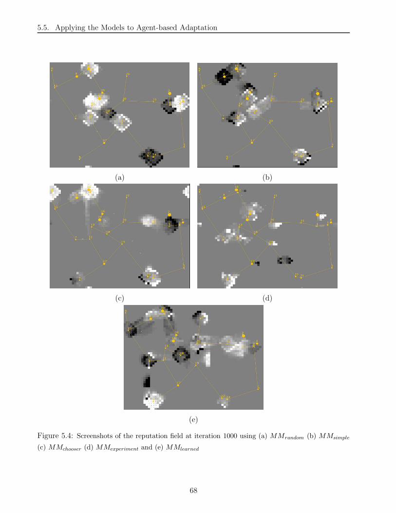
5.5. Applying the Models to Agent-based Adaptation
(a) (b)
(c) (d)
(e)
Figure 5.4: Screenshots of the reputation field at iteration 1000 using (a) MMrandom (b) MMsimple
(c) MMchooser (d) MMexperiment and (e) MMlearned
68

Chapter 6
An Implementation of the Adaptation Framework
This chapter describes in technical detail the design and implementation of the adaptation
simulator used in the experiments described in the previous chapters. We begin with a broad
overview of how adaptation fits into modern games, followed by an analytical breakdown of
the actual adaptation engine. We then describe some tests to evaluate the performance of the
implementation, describe a few optimizations, rerun the tests, and conclude on the quality of
the optimizations.
6.1 Adaptation in Modern Persistent-state Games
The design and implementation of modern multi-player online persistent-state games are heavily
influenced by both the efficiency of the network and efficiency of rendering graphics. Rendering
graphics is for the most part a client-side issue; that is, it depends mostly on the performance
of the computer running the game client. The efficiency of the network, however, is largely
dependent on the infrastructure and the architecture of the game’s network protocol. In these
types of games in particular there is an abundance of information being passed over the network,
and so optimal network performance is a high priority.
By far the most popular architecture in general is the client/server architecture because it
captures the nature of most network tasks and is widely-used. As well, the reliable connection-
oriented Transfer Control Protocol (TCP) fits quite well in the client/server architecture. Stud-
ies show however that the client/server architecture is inadequate for multi-player games because
the large load endured by the server makes the network unscalable. As such, there are current
research projects devoted to optimizing network performance in modern games. For the most
part, these projects stem from the existing algorithms studied in distributed simulation now
69

6.1. Adaptation in Modern Persistent-state Games
...Servers
Clustered
...State
Server
EngineAdaptation
Client
Client
Client
Client
Client
Client Client
Client
Client
Client
ArchitectureDistributed
History
ArchitectureClustered−Server
Figure 6.1: The general layout of the adaptation architecture
evaluated in a game context. Of them, 2 generic alternative architectures have been proposed:
the clustered-server architecture, and the distributed architecture.
Clustered-server architectures try to keep the general layout of the client/server architecture
while trying to reduce the load on a single server. The idea is that there still exists a central
authority, but that central authority may be composed of many computers in a cluster which
are themselves distributed. Example implementations include the mirrored-server architecture
built on Quake in [CFK01], the proxied-server system in [MFW02] and the hierarchical server
architecture found in [Fun96].
Distributed implementations attempt to spread some of the previously server-side processing
computation across client machines. Note that this is fundamentally different than clustered-
server architectures because in this case we are allowing clients access to state information,
which is potentially sensitive. This solves the scalability problem but introduces other problems
such as state inconsistencies, cheating, and load-balancing. Examples include MIMAZE [DG99]
and EternaZ [Qua03].
We would like to extend these architectures now to include the process of adaptation in the
virtual environment. We first introduce a critical concept: the state history server (SHS). The
SHS acts as a global camera: it keeps track of the global state of the game by taking “snapshots”.
It is responsible for collecting state information from clients and/or servers periodically, possibly
re-assembling separated parts of the state to form the global state, storing the history of the
game state, and providing the history of the game state to the adaptation engine. The SHS is
also responsible for sending state updates back to the clients and/or servers as a result of the
adaptation. The general idea is illustrated in Figure 6.1. Note, in particular, that the proposed
logical concept fits into every one of the major network architectures currently used in MMOGs.
70

6.2. Design and Implementation of the Adaptation Engine
In the next section, in fact in this entire chapter, we analyze in detail only the adaptation
engine component of the general architecture. We do not assume that it is trivial to implement
the SHS or the communication between the SHS and the clients and server, but it is outside of
the scope of this research. We focus mainly on proving that the implementation of a modular
and efficient adaptation engine is feasible.
6.2 Design and Implementation of the Adaptation Engine
The adaptation engine is written in Java. Some of the data-gathering and processing tasks where
handled by Perl and shell scripts, but they are not required components. In both languages,
prototyping is easy. Java inherently offers object-oriented principles and supports most popular
design patterns while Perl is superior for lower-level tasks such as parsing data in a particular
format and reporting analyses done on output data from program executions.
Most design concepts mentioned in this section, unless otherwise noted, were taken from
[LG01]. First, I will list the major modules and show the module dependency diagram. Then,
for each module a list of the major components is presented, as well as any non-trivial program-
matical challenges faced in the implementation, algorithms used, and design patterns used.
The engine relies on 2 packages provided externally: hexIT [Lan03] and Minueto [Den04].
hexIT is a Java package that provides an API for using and drawing 2D hexagonal grids.
Minueto is a reasonably efficient gaming and graphics framework for Java which is intuitive to
use.
The major modules are:
• Abstract Simulator
• Plug-in Adaptation Systems
• Abstract Fuzzy Controller
• Abstract Grid API
• Movement Modeling
• Core Utilities and Data Structures
• Conquero
• Game Data Analyzer
71

6.2. Design and Implementation of the Adaptation Engine
SimulatorAbstract
AbstractGridAPI
AbstractFuzzy
Controller
MovementModelling
API
Core Utilities and Data Structures
Conquero
AnalyzerDataGame
SystemsAdaptation
Plugin
Figure 6.2: The module dependency diagram of the implementation
The dependencies between each module and approximate relative size/significance of each
module are given in Figure 6.2.
Abstract Simulator
The abstract simulator module has two major components: the simulation engine, and the
Graphical User Interface (GUI). This module is the largest, most significant part of the entire
implementation. It is essentially the construction of the pseudo-code in Equation 3.1 with many
abstract helper functions.
The GUI component is solely responsible for graphical representation of and user interaction
with the behavior of the simulations. It is composed of 3 sub-components: the Control Panel,
Grid Panel, and Button Panel. The Control Panel allows the user to control the state of
the simulator. The button panel provides buttons that allow the user to dynamically enable
or disable features in the simulation. The grid panel shows the state of the grid during the
simulation and allows the user to inspect and modify the values on the grid dynamically.
The engine component has no subcomponents. It provides the tools which are independent
of the specific adaptation scheme used, such as vector propagation and fuzzy flow-updates.
The component specifies an abstract simloop() method which must be overridden by subclass
plug-ins. The plugins are adaptation systems which have access to the grid and implement
a particular adaptation scheme, as defined in Chapter 4. By keeping this base component
separate from the plugin systems, we allow it to be independently optimized.
One non-trivial challenge was finding the correct set of thread synchronization constraints
between the engine and the GUI: writing code free of non-deterministic behavior while keeping
a certain level of performance. It was also hard to decide what should be part of the abstraction
72

6.2. Design and Implementation of the Adaptation Engine
and what part of the plugins.
Plugin Adaptation Systems
This module consists of 2 major components: the adaptive weather system and the adap-
tive reputation system. There is also a minor component called the aggregate system. Each
component has a separate simulation loop that modifies the grid as detailed in Chapter 4.
The plugin systems have a relatively straight-forward implementation. They each override
the simloop() method specified by the abstract simulator, contain specific code logic particular
to the adaptation system while using as many generic concepts (shared methods from the base
class) as possible to encourage code reuse.
The weather plugin defines 3 main grid-altering methods: moisturewind, gradDev, and
rain. The first displaces moisture between cells based on the current wind vectors. The second
bends the wind vectors towards the gradient vectors. The third displaces moisture directly
based on the gradients. There are 2 extra functions that clear and apply the calculated mask
(separate grid containing grid cell differences, see Section 3.2.1) to the current virtual terrain:
cMask and aMask. Recall from Section 3.2.1 that masks are used to emulate fair simultaneous
updates.
The reputation plugin also has 3 main grid-altering methods: repEvent, agentBend, and
repwind. The first method generates reputation events. The second method shapes the rep-
utation vector field based on the orientations of the agents. The third method spreads the
reputation points based on the values of the reputation vector field. This plugin has similar
mask functions.
The generic adaptation concepts were conceived during the implementation of these plu-
gin systems. The most challenging part of implementation of these components was code
maintenance. Throughout the course of the implementation, these components were the most
actively-modified. The volatility of the code made it somewhat difficult to keep track of the
current functionality.
Abstract Fuzzy Controller
The abstract fuzzy controller module is composed of a set of minor components for representing
arbitrary fuzzy sets and generic tools for operating on these abstractly-defined sets.
To define a particular fuzzy set, the implementor must extend the FuzzySet class and
override the membership(Object) method. The operations provided include those required to
73
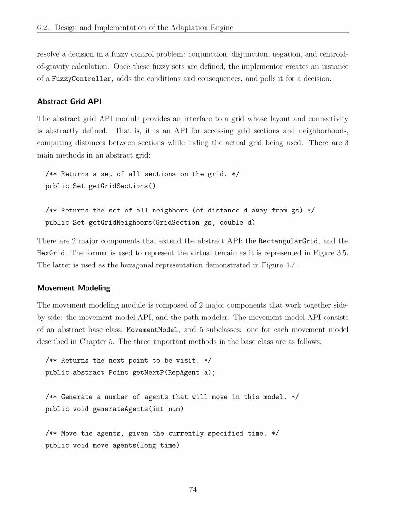
6.2. Design and Implementation of the Adaptation Engine
resolve a decision in a fuzzy control problem: conjunction, disjunction, negation, and centroid-
of-gravity calculation. Once these fuzzy sets are defined, the implementor creates an instance
of a FuzzyController, adds the conditions and consequences, and polls it for a decision.
Abstract Grid API
The abstract grid API module provides an interface to a grid whose layout and connectivity
is abstractly defined. That is, it is an API for accessing grid sections and neighborhoods,
computing distances between sections while hiding the actual grid being used. There are 3
main methods in an abstract grid:
/** Returns a set of all sections on the grid. */
public Set getGridSections()
/** Returns the set of all neighbors (of distance d away from gs) */
public Set getGridNeighbors(GridSection gs, double d)
There are 2 major components that extend the abstract API: the RectangularGrid, and the
HexGrid. The former is used to represent the virtual terrain as it is represented in Figure 3.5.
The latter is used as the hexagonal representation demonstrated in Figure 4.7.
Movement Modeling
The movement modeling module is composed of 2 major components that work together side-
by-side: the movement model API, and the path modeler. The movement model API consists
of an abstract base class, MovementModel, and 5 subclasses: one for each movement model
described in Chapter 5. The three important methods in the base class are as follows:
/** Returns the next point to be visit. */
public abstract Point getNextP(RepAgent a);
/** Generate a number of agents that will move in this model. */
public void generateAgents(int num)
/** Move the agents, given the currently specified time. */
public void move_agents(long time)
74

6.2. Design and Implementation of the Adaptation Engine
x
y
Figure 6.3: An example conversion of a path model
The last 2 methods have a generic implementation that is only overridden by the implementation
of MMexperiment because it must move the agents directly. Otherwise, the movement models
use the generic implementation which chooses a path to take via the path modeler.
The path modeler component is used to design a precise path for the agents to follow when
they are traveling between specific locations in the virtual terrain. The path modeler is another
abstract API which encourages extensibility: the abstract base class PathModel allows for
the implementation of arbitrary two-dimensional parametric curves. It contains 3 important
methods:
/** Construct a path model with given source and destination coordinates. */
public PathModel(int startx, int starty, int endx, int endy)
/** Get the next point on the path at time t, 0 <= t <= 1 */
public Point val(double t)
/** An arbitrarily varying continuous function on the normal Cartesian
plane where val_y(0) = 0 and val_y(1) = 0. */
public abstract double val_y(double t);
The value returned by val(double t) is a point on the virtual terrain at time t assuming the
agent takes a path from its start position to its end position governed by the function val y().
To get this value, a simple change of coordinate systems calculation using affine transformations
is done (see Section 4.2.1). An example of a transformation is given in Figure 6.3.
To emphasize the applicability of the API, several types of path models are implemented:
parabolic, cubic, sinusoidal, quadric, generic polynomial, and composite paths. A PathChooser
object is constructed which generates specific paths needed by the agents. The PathChooser
75

6.2. Design and Implementation of the Adaptation Engine
object follows the factory design pattern.
Core Utilities and Data Structures
This module exists mainly to act as a central resource for providing generally useful objects,
methods, and algorithms. It provides 6 major components: the Utils class, the Debug class,
the discrete probability distribution class, the agent classes, the proximity graph data structure,
and the decision tree data structure.
The Utils class is a collection of static helper methods and also provides the central random
number generator used by all other classes. This allows us to reproduce the exact outcome of
an experiment by simply reusing random seeds.
The debug class allows control of debug information to be printed and/or logged. The
scheme prints no debug information by default (debug level 0) and prints messages whose
detail depend on the debug level set by the programmer. This was particularly helpful when
searching for the cause of erroneous behavior in the implementation.
The discrete probability distribution class provided a means for non-uniform sampling from
a set of predefined objects. The class allows the programmer to add items, each with given
weights attached to them. Then, when drawing from the set, the probability of drawing an
item is equal to its weight divided by the total of all the weights.
The agent classes follow the linguistic relationship: GameAgent is a RepAgent is a SimpleAgent
is an Agent. The first and basic description of an agent is an entity that has a current position
and current velocity, implemented by Agent. When agents were used in more than one system,
SimpleAgent was constructed which contained an extra parameter to specify to which system
the agent belonged. A RepAgent is an agent that contains specific information relevant to
the reputation experiment (ie. its reputation value) and GameAgents contain Conquero-specific
information such as hit points, stamina, and current level.
The proximity graph data structure is an implementation of a regular graph with each vertex
having (x, y) coordinates in a two-dimensional space (in our case, the virtual terrain). A point
in the terrain is represented by the Point object. In the Conquero experiment, this object is
extended to City to represent a command center which has an extra size parameter value, the
Graph class is extended to DirectedGraph. Finally, the Graph object supports special graph
constructions. From just a set of points Graph.RNGize() will construct the graph as its relative
neighbourhood graph. Similarly for Graph.MSTize() and its minimum spanning tree.
The decision tree data structure is an implementation of a binary decision tree. The factory
pattern is used again here because decision trees are only imported via files: they are never
actually constructed by the programmer. This decision tree data structure is created by parsing
76

6.2. Design and Implementation of the Adaptation Engine
the output generated by the C4.5 software [Qui92]. This became a tricky task when large trees
were split into collections of subtrees, because the software used does not represent the textual
output of the full tree. The output of large trees are decomposed into many smaller subtrees
while using annotations to indicate small subtrees. Each subtree is then listed separately.
The algorithm used to overcome this problem is as follows:
1. Collect all the lines of textual data and name for each subtree.
2. Parse each tree individually possibly marking some nodes as degenerate subtree reference
nodes, marking the name of the subtrees to which they should attach in the node. Add
the map (name, tree) to a global hash.
3. Recursively, traverse the base tree depth-first. When a subtree reference node is encoun-
tered, read the name marked on the node and retrieve the corresponding subtree. “Tie”
the subtree to the main tree by replacing the degenerate node by the root of the subtree.
Conquero
Conquero has 3 major components: Minueto, the game client, and the authority server. Minueto
is an external package that was used for its efficient graphics rendering. The game itself is
entirely network-based. It uses a mix of 2 commonly used network protocols: UDP for situations
where efficiency is critical, and TCP for situations where reliability is most critical.
The client first connects (over TCP) to an authority server to validate its requested player
name and IP address. If the IP address is new and the name is already taken by another player
then the connection is rejected. If the name is a duplicate but the IP addresses is the same
one that asked for that name, then the server assumed this is a reconnect and the connection
is accepted. After the server receives the number of players required, the games starts and the
main window spawns.
Critical information such as hits, kills, captures, etc. is passed through the server and
validated by TCP. The server is responsible for ensuring fairness and consistency by imple-
menting locking mechanisms to avoid concurrency problems. Non-critical position updates are
sent via multicast UDP. All clients subscribe to the same multicast IP address and all move
update packets are sent to that address. The result is intended to be a good use of the network
protocols given their advantages and disadvantages.
The authority server does 2 more things other than respond to TCP events. Before starting,
it opens a Java runtime environment and runs a shell script which checks the amount of space
left on the disk partition which used for logging. This ensures that a game experiment will not
77

6.2. Design and Implementation of the Adaptation Engine
fail due lack of disk space for recording game data. Secondly, it also acts as a non-graphical
client. That is, it subscribes to the same multicast address that the clients are connected to
and just logs the packets it receives as well as the TCP packets.
A non-trivial part of the implementation was including dead-reckoning [SZ99]. To implement
dead-reckoning, two important things needed to be considered: a dynamic counter and accurate
synchronized time-stamping. Luckily, the environment used by the game-playing experiment
had synchronized clocks using NTP [Mil85] and hence we assumed an accurate global clock.
The dynamic counter consistently remeasured the rate of updates by averaging the number of
updates it processed in the last fixed interval of time. This provides a window of historical
data suitable for a simple dead-reckoning algorithm: to apply dead-reckoning, the client simply
applies, in one step, a number of updates to the agent which was equal to the update rate
multiplied by the difference between the current time and the timestamp. The resulting position
is the extrapolated position given the agent’s velocity and timestamp. If further updates are
received which contradict any predicted positions, the positions are immediately changed to
reflect the values by the new update, to ensure maximum consistency. Note that applying
immediate correction is the simplest way of dealing with the inconsistencies introduced by
dead-reckoning; researchers have proposed other means, such as Time Warp [Mau00] and linear
convergence [SKH02].
Game Data Analyzer
The game data analyzer module is itself a single component. It is independent of most of
the other logic used in the implementation. It has one general function: to process the data
collected during the game-playing experiment described in Section 5.2.
The data analyzer has 3 important analyses of the data: tofro-stats, tofro-shapes, and tofro-
data. The tofro-stats analysis processes an entire game log and computes overall statistics
above the game log such as the ones found in Table 5.1. This analysis also outputs the data
for the first classification problem explained in Section 5.3.1. The tofro-shapes analysis shows,
graphically, the paths taken by the agents between command centers. The tofro-data analysis
simulates the entire game from the game log for each agent. At every transition of command
centers it also measures the values of the features described in Section 5.3.2 and outputs the
data set for the second classification problem.
78

6.3. Performance Measurements
Name HOME HUMAN TOFU MAGIC
CPUs 1 1 2 4
CPU model Pentium IV AMD Athlon AMD Athlon AMD Opteron
CPU bus width (bits) 32 32 32 64
CPU speed (MHz) 1716 1250 1667 1794
CPU cache size (kB) 256 256 256 1024
Total Memory (kB) 515484 516216 2069368 3613560
Operating System Debian2 Linux Debian2 Linux Debian2 Linux Gentoo Linux
Kernel Version 2.6.5 2.4.26 2.4.20 2.6.7
Table 6.1: Descriptions of the machines used to measure performance.
6.3 Performance Measurements
In this section, we will describe the test environments used for experiments that were run to
measure the performance of various parts of the implementation. The testing environment
includes specifications of hardware used to perform the tests, specification and layout of any
input data/files that were commonly-used, and any relevant miscellaneous information. Then,
each performance test is described individually.
We begin with a descriptions of the environments used to run each test, summarized in
Table 6.1. We will refer to these machines throughout the rest of the chapter.
Existing altitude maps of geographical regions were used as input data for the weather
simulations. The data was obtained using the DIVA-GIS software and information archive
[RHG03]. The number of points in the data set was enormous. This was a problem because
the simulations would span several hundred screens and so was not graphically representable.
The data was reduced by summarizing large portions of the actual data by the average of the
altitude values in the area, as as described in Section 4.1.1.
The first such altitude map to be used was prk alt.dat, a 48x40 altitude map of North
Korea. The other altitude map is pak alt.dat, a 63x51 altitude map of Pakistan. Larger
versions are pak alt2.dat (127x102), pak alt3.dat (255x204), and pak alt4.dat (1022x817).
The reputation simulations load settings from a configuration file called the repfile. Each
repfile contains the number of agents, the graph, the probability of causing events, vertex sizes,
etc. The probability that an event occurs on a given timestep is prEv. The probability that oc-
curred events are good is prEvGood, otherwise they are bad. All reputation simulations use prEv
= 0.001 and prEvGood = 0.7. These numbers were chosen arbitrarily. The test rep3 repfile
2Debian Sarge on HOME and HUMAN , Debian Woody on TOFU .
79

6.3. Performance Measurements
Wtr+GUI Wtr+NOGUI Wtr GUI Rep+GUI Rep+NOGUI Rep GUI
Overhead Overhead
HOME 120.072 76.92 35.94% 40.17 9.92 75.3%
HUMAN 71.88 45.23 37.1% 18.46 7.43 59.75%
Averages 36.52 % 67.53 %
Table 6.2: Data obtained by running performance tests on the graphical interface
uses 20 agents, a random clique graph with 20 vertices of maximum size 12, and a virtual terrain
of 700x700 pixels (50x50 grid cells). test rep3-2 doubles those values: ie. 40 agents, a random
clique graph with 40 vertices of maximum size 24 and a virtual terrain of 1400x1400 (100x100).
Similarly, test rep3-3 doubles the values of test rep3-2 and test rep3-4 quadruples the
values of test rep3.
All performance tests were done on code compiled by Sun’s Java 1.5 compiler and run using
Sun’s Java 1.5 interpreter. All performance tests used the same random seed (= 290423987).
GUI Overhead
The purpose of this test is to measure the average overhead added by the GUI. TOFU and
MAGIC are server machines only accessible via network, and were therefore not used for this
test. This fact is important to know, especially since the machines presented below are more
similar than the server machines. The GUI overhead presented here might be much larger
than what would be observed on more powerful machines. The test runs for 10000 iterations
in the weather simulator with altitude map pak alt.dat and reputation simulator with repfile
test rep3.
The results of the tests are listed in Table 6.2. Based on the observed overheads, it is clearly
inappropriate to do server-side experimenting with the interface enabled. Thus, subsequent
tests do not include the interface components. The interface remains a tool mainly intended
for visually observing the effects of the adaptation process.
Weather Simulations
The purpose of this test is to measure the general performance of the weather simulations. The
weather simulation is run for 10000 iterations on all 4 machines, first on pak alt. Tests on the
larger maps pak alt2, pak alt3 are then run to get a sense of how well the algorithm scales.
The results of the tests are listed in Table 6.3.
Note that average times are calculated over only four and entirely different machines: this
80

6.3. Performance Measurements
is intentional. We would like to summarize the results as to express them in the most general
context possible. That is, while the results per machine are still shown for the most part, we
rely on the average to give a good generic estimate for the results independent of the hardware
used.
If we assume that the time taken per iteration per grid section is constant, then we expect
that the total time taken in one iteration to be a linear function of the number of grid sections.
That is f(G) = k1 + k2 · |G|. Using 3 maps, we get 3 equations:
43.244 = k1 + (63 · 51)k2 (6.1)
177.564 = k1 + (127 · 102)k2 (6.2)
692.77 = k1 + (255 · 204)k2 (6.3)
Solving the system of linear equations 6.1 & 6.2 gives (k1, k2) = (−1.06, 0.013789). Similarly,
solving the system 6.2 & 6.3 gives (k1, k2) = (6.73, 0.0131881). So, it seems that constant
overhead is lost going from maps pak alt.dat to pak alt whereas overhead is added in the case
of going from maps pak alt2 to pak alt3. This could be due to thresholds of memory and cache
being crossed in the second transition, but unfortunately we do not have any memory usage
data to justify this. It is still reassuring that the constants k2 are approximately equal (error
of approximately 6.01 × 10⁻⁴) reinforcing the belief that the performance of the computation
grows linearly.
Tornadoes
The tornado effect is an optional effect included in the weather system. On HOME using
pak alt.dat after 10000 iterations the tornado calculations took on average 1.0389 ms. The
tests were repeated on HUMAN, TOFU, and MAGIC and the results were, respectively: 1.268,
1.188, and 1.185. This gives an average time of 1.17 ms/iteration. If this cost was added to the
current simulations, then it would take 1.1743.244+1.17
= 2.6% of the current total time per iteration.
It is interesting that complex weather effects such as simple tornado simulations do not add
significantly to the overall cost.
Reputation Simulations
The purpose of this test is to measure the general performance of the reputation simulations.
The weather simulation is run for 10000 simulations on all 4 machines, first on repfile test rep3.
81

6.3. Performance Measurements
Map Machine t/iter t[cMask] t[aMask] t[moisturewind] t[gradDev] t[rain]
1 HOME 65.734 0.044 6.32 14.89 38.60 5.88
1 HUMAN 45.226 0.046 4.89 9.72 27.75 2.82
1 TOFU 30.137 0.017 3.35 5.48 19.63 1.66
1 MAGIC 31.879 0.009 2.26 7.68 16.88 5.05
1 (averages) 43.244 0.029 4.21 9.44 25.72 3.85
1 (proportions) — 0.07% 9.7% 21.8% 59.5% 8.9%
2 HOME 261.312 0.177 27.54 59.73 151.26 22.61
2 HUMAN 182.775 0.275 20.45 38.82 112.07 11.16
2 TOFU 138.446 0.116 14.35 28.88 84.28 10.82
2 MAGIC 127.724 0.040 9.21 30.14 68.30 20.034
2 (averages) 177.564 0.152 17.89 39.39 103.98 16.16
2 (proportions) — 0.09% 10.1% 22.2% 58.6% 9.1%
3 HOME 1021.33 0.81 93.81 237.30 599.04 90.37
3 HUMAN 721.029 1.149 79.77 153.4 441.99 44.72
3 TOFU 527.22 0.71 54.24 119.60 338.48 44.19
3 MAGIC 501.498 0.238 36.82 119.30 267.28 77.86
3 (averages) 692.77 0.727 66.16 157.4 411.7 64.3
3 (proportions) — 0.1% 9.55% 22.72% 59.43% 9.28%
Table 6.3: Results of the performance measurements on the weather simulations. All listed times are
in milliseconds (10−3 seconds), and maps used are pak alt# .
82

6.3. Performance Measurements
Map Machine t/iter t[cMask] t[aMask] t[MM] t[repwind] t[aBend] t[repEv]
1 HOME 9.747 0.304 0.686 0.162 8.351 0.196 0.464
1 HUMAN 7.433 0.405 0.883 0.116 5.872 0.139 0.18
1 TOFU 4.677 0.181 0.916 0.1 3.386 0.82 0.012
1 MAGIC 5.477 0.088 0.254 0.061 4.966 0.074 0.034
1 (averages) 6.834 0.245 0.457 0.11 5.644 0.31 0.173
1 (proportions) — 3.6% 6.68% 1.6% 82.6% 4.5% 2.5%
2 HOME 43.864 2.241 2.592 0.315 37.985 0.636 0.093
2 HUMAN 38.3 3.2 3.684 0.235 30.523 0.616 0.045
2 TOFU 18.31 0.728 3.88 0.205 13.292 0.17 0.038
2 MAGIC 23.23 0.335 2.05 0.138 20.492 0.149 0.061
2 (averages) 30.93 1.626 3.05 0.223 25.6 0.393 0.06
2 (proportions) — 5.26% 9.87% 0.7% 82.7% 1.27% 0.2%
3 HOME 158.588 7.366 10.115 0.94 138.75 1.235 0.176
3 HUMAN 134.06 10.184 14.695 0.737 107.271 1.077 0.96
3 TOFU 75.857 3.088 15.59 0.567 56.12 0.416 0.076
3 MAGIC 89.95 1.447 7.69 0.417 79.93 0.325 0.14
3 (averages) 114.6 5.52 12.02 0.665 95.52 0.63 0.34
3 (proportions) — 4.82% 10.5% 0.6% 83.35% 0.55% 0.3%
4 TOFU 1705.474 164.59 246.366 32.767 1257.501 3.954 0.295
4 MAGIC 1498.64 25.895 153.584 27.26 1289.595 1.751 0.554
Table 6.4: Results of the performance measurements on the reputation simulations. All listed times
are in milliseconds (10−3 seconds), and repfiles used are test rep3-# .
Then the test is rerun on the larger field in test rep3-2, test rep3-3 and test rep3-4. The
movement model used in these simulations was MMrandom. The results of the tests are listed
in Table 6.4.
Performing calculations analogous to the ones performed in the weather simulations, we ob-
serve values (k1, k2) = (27.7172, 0.00032128) from repfile test rep3.txt to test rep3-2.txt
and (k1, k2) = (3.04, 0.002789) from repfile test rep3-2 to test rep3-3. This is rather unex-
pected for two reasons. Firstly, the overhead is less in the second case. Secondly, the constant
k2 differs by an order of magnitude, implying either irregularities in the observations or a non-
linear relationship. However, since the values are so small, it is likely that the inaccuracy of
the observed readings are playing a role in the discrepancy.
83

6.3. Performance Measurements
Machine t[MMrandom] t[MMsimple] t[MMchooser] t[MMexperiment] t[MMlearned]
HOME 0.174 0.156 0.201 0.458 1.817
HUMAN 0.122 0.102 0.154 0.444 1.765
TOFU 0.122 0.094 0.13 0.228 1.111
MAGIC 0.067 0.058 0.094 0.167 0.515
(averages) 0.121 0.103 0.145 0.324 1.302
(proportions3) 0.3% 1.12% 1.56% 3.41% 12.44%
Table 6.5: Results of the performance measurements on the different movement models in the rep-
utation simulations. All listed times are in milliseconds (10−3 seconds), and the repfile used was
test rep3 .
Movement Models
The movement model is an optional effect included in the reputation system. The processing
time taken up by the movement models was measured on each system listed and gave the
following averages: 0.121ms for MMrandom, 0.103ms for MMsimple, 0.145ms for MMchooser,
0.324ms for MMexperiment, and 1.302ms for MMlearned. Note that in MMexperiment, the moves
are drawn directly from large input files and not simply generated as the rest.
The tests on repfile test rep6.txt were run for 10000 iterations using MMrandom. test rep6.txt
is a repfile recreation of the terrain and graph used in the Conquero game-playing experiment.
This test was repeated on each machine but using different movement models. The results for
the movement models are summarized by Table 6.5.
As expected, the learned model takes the longest because it calculates the value of 232
features based on the current state, pass these through a decision tree, and then make a decision.
The random and simple models are low because they do not do any processing of the current
state. The chooser model only slightly less efficient than the simple model, which is encouraging
considering it is calculating the value of 3 heuristics and passing through a decision tree. The
inefficiency of the experiment model is due to the fact that it is reading its moves from a large
(83M) log file.
3of total average time taken per iteration taken from Table 6.4
84

6.4. Optimizations
6.4 Optimizations
In this section, we will describe optimizations designed to improve the performance of the
implementation. Each optimization will then be evaluated by re-running tests with the opti-
mization enabled and compared to the values obtained in the previous section. First, minor
optimizations are suggested. Then the larger, more significant optimizations are described in
their own subsections.
One simple optimization is to use tabular look-up approximations for trigonometric functions
sine and cosine. The optimization upon startup inserts the values of sine and cosine in a table
for 1000 · 2π values (0.000 · 2π to 1.000 · 2π). In fact, only one table need be stored since
cos(x) = sin(x + π2). Larger angles are mapped by repeatedly adding or subtracting 2π until
the angle is in the desired interval. Then, the true values are linearly extrapolated between the
two approximate values contained in the lookup tables.
The first weather simulations we rerun using this optimization. An improvement was ex-
pected, especially since the weather simulations use trigonometric functions more than the
other two systems. The observed average times per iteration are: 63.667 ms, 43.93 ms, 37.116
ms, and 31.142. This gives an average of value of 43.964 ms, slightly (1.7%) higher than the
unoptimized result. Therefore, it is clear that Java must be doing something efficient in their
Math class to save on execution time.
6.4.1 Caching
Caching is a common optimization technique used throughout Computer Science. The general
idea is to remember a value once it is calculated so that future calculations need only read the
cached value rather than recompute the value repeatedly. Note that caching really just trades
space (memory) for time (performance). It is usually the case that the trade-off is worth doing
when the programmer expects a given calculation to be repeatedly calculated.
There is one obvious application of caching in the weather system: gradient-caching. The
gradient need not be re-calculated unless it changes. In fact, this is a general optimization
technique that can be applied to all environment-based adaptation schemes since the influence
of the adaptation is based on the environment which we expect to change little. However, this
optimization does add a bit of programmatical complexity. This is because the programmer is
forced to take care of the special case of when the gradient vectors change.
To measure the value of this optimization, the first set of weather simulations were once
again rerun. The average times per iteration observed is: 55.87, 36.53 ms, 25.86 ms, and 28.81
ms. This gives an average of 36.77 ms per iteration, corresponding to a 15% improvement. This
85

6.4. Optimizations
is an encouraging, significant result.
6.4.2 Concurrency
A natural optimization for computations on discrete grid cells is parallelization. In our case, we
do not have access to powerful parallel machines, but we can emulate the idea of parallelization
through software and hardware using concurrency and multiple processors.
A multi-threaded version of the weather simulation loop is implemented. The multi-threaded
version simply partitions the grid into independent portions, and assigns the responsibility of
carrying out the calculations for that portion to each thread independently of the other threads.
At every iteration, the threads perform the grid-base calculations concurrently and then wait
while a central thread applies global duties such as clearing and applying the mask.
The threads were synchronized by using a typical n-process barrier mechanism, where n ∈
{1, 2, 3, 4}. The synchronization code is outlined in Figure 6.4. Two counting semaphores and
2 boolean condition variables were used in the n worker threads and single main thread. The
workers performed the adaptation procedures on the a section of the grid while the main thread
performed the global procedure and thread management. One important note is that Java’s
built-in concurrency features such as monitors and object locks were used.
The purpose here is to find a partition of the terrain that is intuitive, easy to compute, and
splits the region into subregions of equal area. If 2 (or 3) threads were invoked, then the terrain
was split into 2 (or 3) rectangular regions by taking the longest side and finding the midpoint
(or the one third and two third points) and then using the perpendicular bisector of the edge
at that point as a new boundary between split regions. The 4-thread version split the region
into 4 quadrants similarly, but uses the midpoints of each side inside of just the longest side.
The weather tests were rerun on the multi-processor machines TOFU and MAGIC. In this
case, all the tests were rerun so that the effect of larger maps on the concurrent implementation
could be found. The results of the simulations are listed in Table 6.6.
There are some comments to make on these observations. Firstly, it seems odd that dual-
processor (TOFU) performs better than quad-processor (MAGIC) when using 4 threads on 2
out of the 3 maps. From Table 6.1, we notice that the speeds of the processors are approximately
equal, and that MAGIC has twice the amount of memory that TOFU has. Therefore, it seems
likely that the different major versions of the Linux kernel (2.6.x vs 2.4.x) could be the culprit.
It would be interesting to investigate this further.
4compared to the single-thread version.5the value of
tsinglethread
tmultithreador simply proportion−1
86
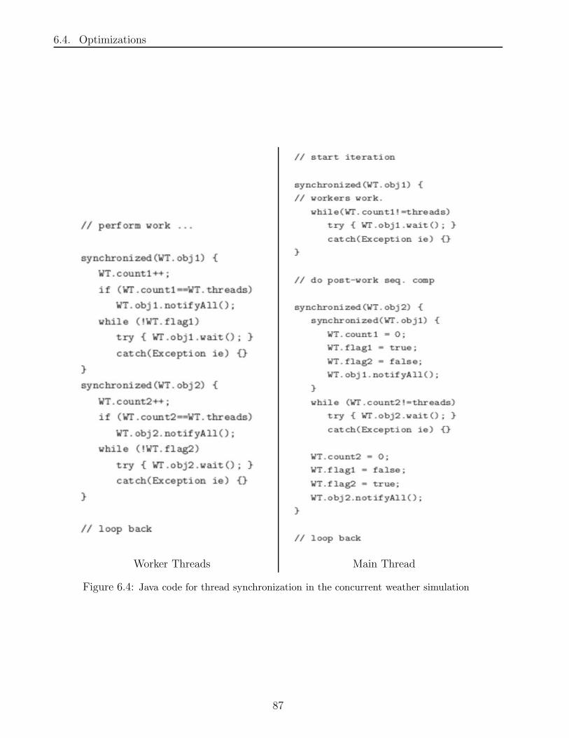
6.4. Optimizations
Worker Threads Main Thread
Figure 6.4: Java code for thread synchronization in the concurrent weather simulation
87

6.4. Optimizations
Map Machine # of threads t/iter Improvement4 Proportion4 Speed-up5
1 TOFU 2 18.94 11.197 63% 1.59
1 TOFU 3 14.76 15.377 49% 2.042
1 TOFU 4 12.37 17.767 41% 2.4363
1 MAGIC 2 19.964 11.92 63% 1.597
1 MAGIC 3 17.462 14.417 55% 1.826
1 MAGIC 4 16.9 14.979 53% 1.89
2 TOFU 2 79.623 58.823 58% 1.74
2 TOFU 3 62.706 75.74 45% 2.21
2 TOFU 4 55.175 83.271 40% 2.51
2 MAGIC 2 83.027 43.973 65% 1.54
2 MAGIC 3 72.803 54.921 57% 1.7544
2 MAGIC 4 66.53 61.194 52% 1.92
3 TOFU 2 315.843 211.377 60% 1.67
3 TOFU 3 316.693 210.527 60% 1.665
3 TOFU 4 332.908 194.312 63% 1.584
4 MAGIC 2 325.13 176.368 65% 1.54
4 MAGIC 3 273.93 227.568 55% 1.83
4 MAGIC 4 271.09 230.408 54% 1.85
Table 6.6: Results of the concurrent weather simulation tests. All listed times are in milliseconds
(10−3 seconds), and the altitude maps used were pak alt#.
88

6.4. Optimizations
Secondly, when running the weather simulation test on pak alt3.dat adding threads on
TOFU seems to slow down the process instead of speed it up, but this does not happen on
MAGIC. This implies that TOFU has reached some kind of threshold: either concurrent mem-
ory access is slowed down due to the fact that there is a lot of information being stored in
memory and the cache memory becomes filled too quickly, or the amount of memory is too
much to hold in RAM so virtual memory is used in which case a lot of overhead is added for
swapping information in and out from secondary memory.
We now use these observed values to approximate how much of the weather simulation
computation is due to sequential (single-threaded) computation versus parallel (multi-threaded)
computation. As a tool to help us measure the influence of these two separate values, we use
Amdahl’s Law [Amd67]:
speedup =1
(1− p) + pn
(6.4)
where speedup is the best possible attained speedup, p is the proportion of time spent in the
parallel part of the program, n is the number of processors, s is the proportion of time spent
in the sequential part of the program, and s + p = 1.
Using 2.51 as the best speedup attained on 2 processors, we get p = 1.2032. There are
other instances for which TOFU beats its theoretical maximum: both when using more than
2 threads on the first 2 maps. This means that on TOFU we are experiencing superlinear
speedup [HM89]; it is sometimes when multiple CPUs are used and is typically due to the
effects of processor caches. In these cases, so we cannot use these exceptional cases to find the
values we are interested in.
In the case of the third map, the max speedup obtained by TOFU is 1.67. In this case, we
obtain (p, s) = (0.8, 0.2). The same calculations are repeated for MAGIC in all 3 cases and the
values obtained are: p = 0.63, p = 0.64, and p = 0.613. This gives an average of p = 0.67 and
s = 0.33. Therefore, roughly one third of the time in the concurrent implementation is spent
doing sequential computation.
6.4.3 Buffering
The buffering technique proposed here is similar to the double-buffering [FvDFH95] technique
that has been widely-applied in the domain of Computer Graphics. The core concept involves
holding two objects (buffers) in memory: a scrap buffer and a display buffer. The application
works on the scrap buffer while displaying the display buffer to the user. When the application
has done the work it needs, the roles of the 2 buffers are interchanged. Typically, switching
the roles of these 2 buffers is a very efficient process, more efficient than working on the same
89

6.4. Optimizations
buffer that is being displayed. As a result, a performance improvement is generally observed.
Here, a similar strategy is used. There are 2 buffers: one called the write buffer and the
other called the read buffer. The write buffer is never displayed, only modified. The read buffer
displayed and inspected by the main algorithms. Both buffers hold a single independent grid.
Initially, the two buffers are created and are identical. Each iteration, the algorithms inspect
the read buffer and calculate all changed needed to be done, but instead apply the changes to
the write buffer directly instead of temporarily storing the values in a mask and applying the
mask later. Before the next iteration begins, the roles of the two buffers are switched so that
the read buffer then contains the grid with recently-modified values.
When the simulations enable buffering, the methods that modify the values of the state
do so directly to the write buffer. Therefore, Buffering effectively allows the removal of the
applyMask and clearMask functions and so should have an effect on the performance.
The obtained results for average time per iteration on the weather simulations were 69.96ms,
47.72ms, 33.32ms, 32.01ms, giving an average of 45.75 ms/iteration. The time taken per iter-
ation including buffering takes 2.5ms longer. These results clearly conclude that the memory
requirements added to help gain performance have slowed down the implementation enough to
make the optimization not worth including.
6.4.4 Aggregation
Two major application systems have been implemented (weather and reputation) that are
somewhat similar in that they are based on the the same iterative adaptation scheme and data
representation (grid layout). The performance of each individual system has been measured
independently and in several different environments. As well, all optimizations have focused
on improving performance of an individual system or part of a system. All performance com-
parisons have been done on the previous recorded results of the simulations runs using those
systems.
A simple optimization is proposed to combine the simulations to create an aggregate sim-
ulation which uses the same grid and a merged simulation loop which uses algorithms from
both systems separately but on a shared grid. Since the plugin-systems have a simple interface,
integrating many of them in a single simulation engine is quite easy. The interface for each al-
gorithm in a plugin-system is just a method that takes the coordinate positions to be updated
and performs the computation. All that is required by the aggregate simulator is to create
an object of the plugin-system’s type, and to include invocations of the required algorithms
provided by the plugin-system on the plugin object.
90

6.4. Optimizations
Once again simulations were run and performance data collected from them. Map 1 was
used for weather and test rep3.txt for reputation. The average time per iteration on the 4
different machines was: 72.94ms, 53.18ms, 35.08ms, and 31.17ms. The average value is 48.08
ms/iteration. The sum of the averages that were done independently is 43.244+6.834 = 50.078.
This corresponds roughly to a 4% improvement.
The improvement offered by aggregating the two systems is rather small, but not negligible.
This might be due to the fact that we are only combining the iterative process and the grid
not the actual data nor the procedures themselves. Combining the data and procedures would
be removing in part from the usefulness of the plug-in abstraction. In a commercial game,
sharing a grid between multiple systems is a must. This aggregate model proves that multiple
adaptation schemes can easily be contained in the same virtual environment.
We introduced this chapter with an explanation and demonstration of the integration of
the general adaptation scheme into the context of modern persistent-state computer games.
Adaptation of weather and reputation are examples of adaptation schemes that we might find
in such games. The integration of adaptation in the software design sense gives a practical
justification for the usefulness of these schemes.
The basic structure of the plug-in systems and logical control flow were described in Chap-
ter 4. Here, we extended these ideas by a thoroughly detailed breakdown of the actual im-
plementation of the simulator. Since the implementation is modular, creating new modules is
straight-forward.
Performance was measured by running the simulator and tracking the times spent in certain
methods. The two major systems’ performances were analyzed in detail on several different
testing environments. The average was used to reduce and local error or bias cause by a
particular testing environment.
Several optimizations were proposed. The simulations were rerun with these optimization
enabled so as to allow us to quantify the value of an optimization. Some of the optimizations
failed (enabling the optimization lead to slower simulations) and some succeeded. In particular,
concurrency and caching seemed to help out a lot (45% and 15% improvement repsectively) and
system aggregation helps out a small amount (4%). Buffering and simple tabular trigonometric
functions proved to be not worthwhile.
The implementation here is generic enough that any plug-in system could literally be
dropped in to the framework and used. To summarize, the adaptation framework used here is
versatile, robust, and extendible.
91

Chapter 7
Future Work and Conclusions
In this thesis, we have described a generic adaptation scheme for modeling and designing
adaptive virtual environments in persistent-state computer games. Our adaptation model is
composed of several familiar computational formalisms such as data flow and cellular automata.
The model implicitly provides the notion of locality for large-scale environments.
The model enforces a discrete timeline upon which the iterative update cycle is built. This
update cycle defines generic adaption process because it contains a list of abstractly-defined
adaptation procedures. This procedural abstraction allows for specific functional adaptation al-
gorithms to be separately implemented and maintained. Specific adaptive virtual environments
are simply defined by the cellular properties and adaptation algorithms. The simulator can be
used to test each adaptive virtual environment completely independently. Merging adaptive
virtual environments in one aggregate adaptive virtual environment is as simple as including
all the specific procedures in the list to be run by the update cycle.
The model described is generic and intuitive. It is meant to be used by game designers
who are interested in building an adaptive virtual environment in their game. Two adaptation
systems are explained in detail, which serve as a good stepping stones for a designer who would
like to model his/her own different adaptive virtual environment.
The two example systems use some generic adaptation concepts that would likely be re-
used in future systems as well. Local averaging helps distribute the impact of sharp changes
to surrounding neighbors. Using flow as a means for quantified information dispersal is also
a good way to spread the influence of events to surrounding neighbors. Both were used and
demonstrated to work in the example systems.
The entities inside of a virtual environment are really what make the environment react
since entities are allowed to interact in the system. The evolution of the adaptive virtual
environment is then non-deterministic because the entities here will be mostly player characters.
92

The interaction with an adaptive environment adds a significant importance to the player
characters’ actions because they can cause an event that can change the environment forever.
As such, this encourages a real history of the world to develop over time, and players to be part
of a dynamic, realistic world.
As an extension to agent-based adaptation, movement models for mobile agents in game
environment simulations were investigated. The aim was to build a probabilistic model for
agent movement behavior. Specifically, a multi-player network computer game was designed
for a game-playing experiment which collected data to analyze.
The game, called Conquero, involved short range combat and team capture of command
centers. Simple heuristics for movement information were proposed solely based on size of
the next command center and distance from the next command center. The values of the
heuristics were placed into a classification system to see if they were sufficient for deciding
which command center to visit next. The heuristics were extended to include many other kinds
of data prominent in Conquero, such as data that is dynamic like properties of other agents.
Dynamic agents were built by providing the agents with decision trees that were learned from
the dynamic features. Since the computation of these dynamic features was very efficient,
incorporating learning features based on decision-tree classification is likely feasible. In the
context of Conquero, five movement models were described after analyses were performed.
The movement models proposed were re-applied to the reputation system to see what kind
of reputation fields they would give. Interesting results appeared. Using the same seed for the
central random number generator, the 5 models produced quite different results, as confirmed
by Figure 5.4 and Table 5.4.
The performance of the movement models was generally quite good. In particular, the
decision-tree learning method seems to be computationally efficient and serves as a structure for
agent decision-making quite well. However, domain-specific heuristics are required to transform
observed sensory data into something meaningful, implying that some form of knowledge will
have to be pre-programmed even into learning agents.
Finally, we have shown that the use of the adaptation scheme is feasible and suggested an
architecture for applying the the process in modern computer game projects. We have showed
that all the concepts given fit easily into the object-oriented paradigm, allowing for modular
design, code reuse, and easy future modification.
Both the efficiency and performance of the simulations are encouraging. Even at the worse
case scenario, the iterations never took longer than 1 second in total. Considering that adap-
tation is a long-term effect, this level of performance is quite acceptable. We have further give
93

7.1. Future Work
experimental evidence of the effect of some simple optimizations. In fact, some of the perfor-
mance improvements are impressive and encouraging. Other than the caching of the gradient,
the optimizations were independent of the application system.
After all is considered, it seems that adaptive virtual environments are interesting to study
and would add an entertaining new element to a game-player’s gaming experience. It remains
to be seen if players themselves would enjoy playing their character in such environments. We
suspect this new feature would be enjoyable for the most part, since it has been proven in the
game development industry that players enjoy new content. We are hoping, if not expecting,
to soon see adaptive virtual environments in commercial persistent-state games.
7.1 Future Work
There is a good amount of potential for future work on adaptive virtual environments. We will
list the most interesting here and describe each briefly.
Improved Adaptation Systems
The 2 systems proposed in Chapter 4 are quite basic systems. For instance, the weather system
is missing some key elements for it to be realistic, such as temperature, evaporation, growth of
vegetation, atmospheric pressure and so on. Implementing some of the weather events suggested
in the chapter on these applications, such as tsunamis, earthquakes, floods, etc. would also be
another way of improving the existing implementation. Although, adding such feature would
also add complexity and cost.
In the reputation system, it would be nice to implement support for the reputation groups
and membership values. A better movement model is needed than the random one supplied.
Ultimately, it needs to have a movement model that corresponds to real movements of players
in persistent-state games.
Other Adaptation Applications
We have proposed and analyzed two adaptation applications that could be applied in modern
games. There are, of course, many other possibilities for applying adaptation in computer
games.
One rather obvious application is an adaptive economy. An adaptive economy based on
supply and demand could be implemented by flowing information and resource availability
through the grid. Values of items would adapt over time and location, which would change
94

7.1. Future Work
the prices of items sold by vendors. Events in this system could be inflation, theft, or sudden
loss/gain of resources. For example, a forest fire causes a drop in wood supply.
It would also be beneficial if social aspects of environments such as law, politics, etc. could
be quantified. For example, one could envision an adaptive law enforcement system. Crime
would be a measurable scalar property. The amount of law enforcement per region would also
be a scalar property that would adapt to the crime rate of the region. As a result, in the long
run more law enforcers would surround the areas with higher crime, causing the crime rate to
go back down.
Grid Partitioning
In large-scale environments, the virtual environment terrains might not necessarily be rectangu-
lar. Most of these games in fact are using the notion of “zones,” arbitrary but strict partitions
of some larger world. These often correspond to management by separate servers, and so there
can be significant inter-zone communication costs. Arbitrary decomposition into zones can also
of course produce an overall world shape that may not easily map to a regular grid.
Zones, however, are still typically quite large and can contain up to 1000 characters. This
may make it reasonable to adapt zones separately, perhaps with a relaxed consistency model
between zone borders.
Integration of Adaptation Architecture in a Large Persistent-state Computer Game
In Chapter 6, the implementation of the adaptation engine part of the entire adaptation archi-
tecture was shown in detail. The simulators show the adaptation engine running the adaptation
process on the example systems. However, the state history server was not implemented and
remains a future project.
Ideally, an existing game project that is somewhat well-known could be modified so that
it would simply dump information to the state history server and accept modifications from
the state history server. This server would be responsible for collecting data and storing it
in an efficient way, communicating with the adaptation server, and assigning changes back to
the game servers and/or clients. The important part of this future consideration is to have a
sufficiently large player base for the game.
95

7.1. Future Work
The Conquero Experiment, Revisited
Due to resource constraints, Conquero was intended to be an approximate microscopic version
of the events that happened over longer periods of time in a larger persistent-state multi-
player game. However, the game is small, simple and dynamic. As well, its overhead view
allows players to see the entire state of the game at all times. It forces players to remain near
command centers instead of accurately modeling behavior based on player interest. Movement
models could also be improved.
An interesting venture would be to recreate the Conquero experiment using an existing
multi-player game, or even better an existing persistent state game. The benefits of this would
be that the data would reflect the actual constraints of a more representative game interface.
A Generic Model for Adaptive Agents
The movement model learning done in Chapter 5 could also be applied to agents online, during
the game. The decision tree construction was computationally efficient, and so this makes it
possible to implement a movement model where the decision tree is built and used incremen-
tally and dynamically. In fact, we need not restrict the learning agents to decisions based on
movement. Agents could collect a set of data via predefined sensors, calculate the value of
predefined heuristic functions, build a classification problem, solve it, and then use the solution
to make a decision from a set of predefined actions. The adaptation process here would be to
simply recreate the decision tree every so often as to keep it up-to-date from new observations.
96

Appendix A
Learned Decision Tree
The following is a text representation of the decision tree learned from the second classifi-
cation problem described in Chapter 5:
C4h3 <= 4.36315E-5 :| oldCity = 1.0 : 14 (0.0)| oldCity != 1.0 :| | oldCity = 2.0 : 14 (0.0)| | oldCity != 2.0 :| | | oldCity = 3.0 : 14 (0.0)| | | oldCity != 3.0 :| | | | oldCity = 4.0 : 14 (0.0)| | | | oldCity != 4.0 :| | | | | oldCity = 5.0 : 14 (0.0)| | | | | oldCity != 5.0 :| | | | | | oldCity = 19.0 : 14 (0.0)| | | | | | oldCity != 19.0 :| | | | | | | oldCity = 20.0 : 14 (0.0)| | | | | | | oldCity != 20.0 :| | | | | | | | oldCity = 21.0 : 14 (0.0)| | | | | | | | oldCity != 21.0 :| | | | | | | | | oldCity = 22.0 : 14 (0.0)| | | | | | | | | oldCity != 22.0 :| | | | | | | | | | oldCity = 23.0 : 14 (0.0)| | | | | | | | | | oldCity != 23.0 :| | | | | | | | | | | oldCity = 24.0 : 14 (0.0)| | | | | | | | | | | oldCity != 24.0 :| | | | | | | | | | | | oldCity = 6.0 :| | | | | | | | | | | | | C18nop > 23.0 : 7 (3.0)| | | | | | | | | | | | | C18nop !> 23.0 :| | | | | | | | | | | | | | C11nte > 3.0 : 8 (3.0)| | | | | | | | | | | | | | C11nte !> 3.0 :| | | | | | | | | | | | | | | C10nop > 23.0 : 8 (3.0)| | | | | | | | | | | | | | | C10nop !> 23.0 :| | | | | | | | | | | | | | | | C14nop <= 24.0 :| | | | | | | | | | | | | | | | | C16nop > 0.0 : 8 (2.0)| | | | | | | | | | | | | | | | | C16nop !> 0.0 :| | | | | | | | | | | | | | | | | | mopx <= 699.231 :| | | | | | | | | | | | | | | | | | | C13nop > 24.0 : 8 (2.0)| | | | | | | | | | | | | | | | | | | C13nop !> 24.0 :| | | | | | | | | | | | | | | | | | | | vy <= -0.011 :| | | | | | | | | | | | | | | | | | | | | mopx <= 658.923 : 8 (4.0)| | | | | | | | | | | | | | | | | | | | | mopx !<= 658.923 : 15 (2.0)| | | | | | | | | | | | | | | | | | | | vy !<= -0.011 :| | | | | | | | | | | | | | | | | | | | | cto <= 7.0 : 15 (14.0)| | | | | | | | | | | | | | | | | | | | | cto !<= 7.0 :| | | | | | | | | | | | | | | | | | | | | | C17dist <= 365.121 : 11 (2.0)| | | | | | | | | | | | | | | | | | | | | | C17dist !<= 365.121 : 15 (3.0)| | | | | | | | | | | | | | | | | | mopx !<= 699.231 :| | | | | | | | | | | | | | | | | | | mopx <= 736.87 : 13 (2.0)| | | | | | | | | | | | | | | | | | | mopx !<= 736.87 : 8 (2.0)| | | | | | | | | | | | | | | | C14nop !<= 24.0 :| | | | | | | | | | | | | | | | | mopx <= 658.923 : 10 (2.0)| | | | | | | | | | | | | | | | | mopx !<= 658.923 : 8 (2.0)| | | | | | | | | | | | oldCity != 6.0 :| | | | | | | | | | | | | oldCity = 7.0 :| | | | | | | | | | | | | | C17nop <= 0.0 :| | | | | | | | | | | | | | | C24nop > 21.0 : 5 (3.0)| | | | | | | | | | | | | | | C24nop !> 21.0 :| | | | | | | | | | | | | | | | C10nop <= 24.0 :| | | | | | | | | | | | | | | | | C11dist <= 430.094 :| | | | | | | | | | | | | | | | | | C8nte > 3.0 : 15 (3.0)| | | | | | | | | | | | | | | | | | C8nte !> 3.0 :| | | | | | | | | | | | | | | | | | | C15nte > 3.0 : 15 (2.0)| | | | | | | | | | | | | | | | | | | C15nte !> 3.0 :| | | | | | | | | | | | | | | | | | | | C16nte > 6.0 : 13 (2.0)| | | | | | | | | | | | | | | | | | | | C16nte !> 6.0 :| | | | | | | | | | | | | | | | | | | | | mtpx <= 672.667 :| | | | | | | | | | | | | | | | | | | | | | C12nop > 0.0 : 8 (2.0)| | | | | | | | | | | | | | | | | | | | | | C12nop !> 0.0 :| | | | | | | | | | | | | | | | | | | | | | | C9nop > 24.0 : 8 (2.0)| | | | | | | | | | | | | | | | | | | | | | | C9nop !> 24.0 :| | | | | | | | | | | | | | | | | | | | | | | | dco <= 5.0 : 8 (3.0)
97
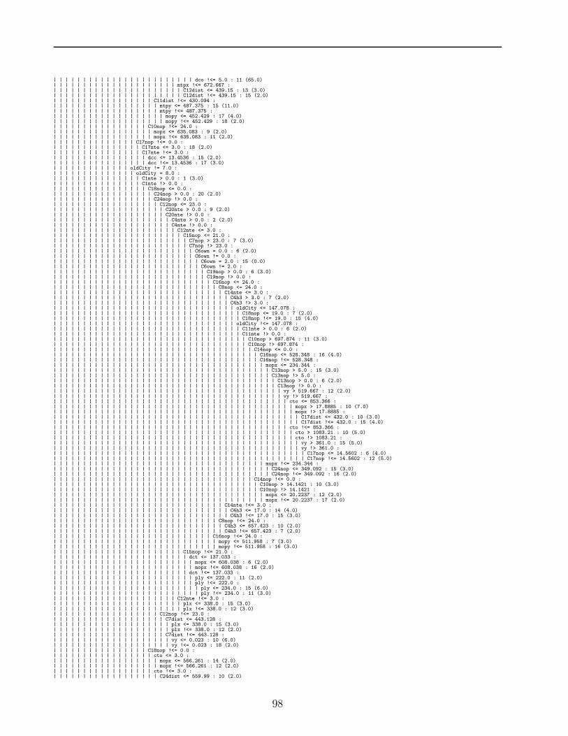
| | | | | | | | | | | | | | | | | | | | | | | | dco !<= 5.0 : 11 (65.0)| | | | | | | | | | | | | | | | | | | | | mtpx !<= 672.667 :| | | | | | | | | | | | | | | | | | | | | | C12dist <= 439.15 : 13 (3.0)| | | | | | | | | | | | | | | | | | | | | | C12dist !<= 439.15 : 15 (2.0)| | | | | | | | | | | | | | | | | C11dist !<= 430.094 :| | | | | | | | | | | | | | | | | | mtpy <= 487.375 : 15 (11.0)| | | | | | | | | | | | | | | | | | mtpy !<= 487.375 :| | | | | | | | | | | | | | | | | | | mopy <= 452.429 : 17 (4.0)| | | | | | | | | | | | | | | | | | | mopy !<= 452.429 : 18 (2.0)| | | | | | | | | | | | | | | | C10nop !<= 24.0 :| | | | | | | | | | | | | | | | | mopx <= 635.083 : 9 (2.0)| | | | | | | | | | | | | | | | | mopx !<= 635.083 : 11 (2.0)| | | | | | | | | | | | | | C17nop !<= 0.0 :| | | | | | | | | | | | | | | C17nte <= 3.0 : 18 (2.0)| | | | | | | | | | | | | | | C17nte !<= 3.0 :| | | | | | | | | | | | | | | | dcc <= 13.4536 : 15 (2.0)| | | | | | | | | | | | | | | | dcc !<= 13.4536 : 17 (3.0)| | | | | | | | | | | | | oldCity != 7.0 :| | | | | | | | | | | | | | oldCity = 8.0 :| | | | | | | | | | | | | | | C1nte > 0.0 : 1 (3.0)| | | | | | | | | | | | | | | C1nte !> 0.0 :| | | | | | | | | | | | | | | | C18nop <= 0.0 :| | | | | | | | | | | | | | | | | C24nop > 0.0 : 20 (2.0)| | | | | | | | | | | | | | | | | C24nop !> 0.0 :| | | | | | | | | | | | | | | | | | C12nop <= 23.0 :| | | | | | | | | | | | | | | | | | | C20nte > 0.0 : 9 (2.0)| | | | | | | | | | | | | | | | | | | C20nte !> 0.0 :| | | | | | | | | | | | | | | | | | | | C4nte > 0.0 : 2 (2.0)| | | | | | | | | | | | | | | | | | | | C4nte !> 0.0 :| | | | | | | | | | | | | | | | | | | | | C12nte <= 3.0 :| | | | | | | | | | | | | | | | | | | | | | C15nop <= 21.0 :| | | | | | | | | | | | | | | | | | | | | | | C7nop > 23.0 : 7 (3.0)| | | | | | | | | | | | | | | | | | | | | | | C7nop !> 23.0 :| | | | | | | | | | | | | | | | | | | | | | | | C6own = 0.0 : 6 (2.0)| | | | | | | | | | | | | | | | | | | | | | | | C6own != 0.0 :| | | | | | | | | | | | | | | | | | | | | | | | | C6own = 2.0 : 15 (0.0)| | | | | | | | | | | | | | | | | | | | | | | | | C6own != 2.0 :| | | | | | | | | | | | | | | | | | | | | | | | | | C19nop > 0.0 : 6 (3.0)| | | | | | | | | | | | | | | | | | | | | | | | | | C19nop !> 0.0 :| | | | | | | | | | | | | | | | | | | | | | | | | | | C16nop <= 24.0 :| | | | | | | | | | | | | | | | | | | | | | | | | | | | C8nop <= 24.0 :| | | | | | | | | | | | | | | | | | | | | | | | | | | | | C14nte <= 3.0 :| | | | | | | | | | | | | | | | | | | | | | | | | | | | | | C4h3 > 3.0 : 7 (2.0)| | | | | | | | | | | | | | | | | | | | | | | | | | | | | | C4h3 !> 3.0 :| | | | | | | | | | | | | | | | | | | | | | | | | | | | | | | oldCity <= 147.078 :| | | | | | | | | | | | | | | | | | | | | | | | | | | | | | | | C18nop <= 19.0 : 7 (2.0)| | | | | | | | | | | | | | | | | | | | | | | | | | | | | | | | C18nop !<= 19.0 : 15 (4.0)| | | | | | | | | | | | | | | | | | | | | | | | | | | | | | | oldCity !<= 147.078 :| | | | | | | | | | | | | | | | | | | | | | | | | | | | | | | | C11nte > 0.0 : 6 (2.0)| | | | | | | | | | | | | | | | | | | | | | | | | | | | | | | | C11nte !> 0.0 :| | | | | | | | | | | | | | | | | | | | | | | | | | | | | | | | | C10nop > 697.874 : 11 (3.0)| | | | | | | | | | | | | | | | | | | | | | | | | | | | | | | | | C10nop !> 697.874 :| | | | | | | | | | | | | | | | | | | | | | | | | | | | | | | | | | C14nop <= 0.0 :| | | | | | | | | | | | | | | | | | | | | | | | | | | | | | | | | | | C16nop <= 528.348 : 16 (4.0)| | | | | | | | | | | | | | | | | | | | | | | | | | | | | | | | | | | C16nop !<= 528.348 :| | | | | | | | | | | | | | | | | | | | | | | | | | | | | | | | | | | | mopx <= 234.344 :| | | | | | | | | | | | | | | | | | | | | | | | | | | | | | | | | | | | | C13nop > 5.0 : 15 (3.0)| | | | | | | | | | | | | | | | | | | | | | | | | | | | | | | | | | | | | C13nop !> 5.0 :| | | | | | | | | | | | | | | | | | | | | | | | | | | | | | | | | | | | | | C13nop > 0.0 : 6 (2.0)| | | | | | | | | | | | | | | | | | | | | | | | | | | | | | | | | | | | | | C13nop !> 0.0 :| | | | | | | | | | | | | | | | | | | | | | | | | | | | | | | | | | | | | | | vy > 519.667 : 12 (2.0)| | | | | | | | | | | | | | | | | | | | | | | | | | | | | | | | | | | | | | | vy !> 519.667 :| | | | | | | | | | | | | | | | | | | | | | | | | | | | | | | | | | | | | | | | cto <= 853.366 :| | | | | | | | | | | | | | | | | | | | | | | | | | | | | | | | | | | | | | | | | mopx > 17.8885 : 10 (7.0)| | | | | | | | | | | | | | | | | | | | | | | | | | | | | | | | | | | | | | | | | mopx !> 17.8885 :| | | | | | | | | | | | | | | | | | | | | | | | | | | | | | | | | | | | | | | | | | C17dist <= 432.0 : 10 (3.0)| | | | | | | | | | | | | | | | | | | | | | | | | | | | | | | | | | | | | | | | | | C17dist !<= 432.0 : 15 (4.0)| | | | | | | | | | | | | | | | | | | | | | | | | | | | | | | | | | | | | | | | cto !<= 853.366 :| | | | | | | | | | | | | | | | | | | | | | | | | | | | | | | | | | | | | | | | | cto > 1083.21 : 10 (5.0)| | | | | | | | | | | | | | | | | | | | | | | | | | | | | | | | | | | | | | | | | cto !> 1083.21 :| | | | | | | | | | | | | | | | | | | | | | | | | | | | | | | | | | | | | | | | | | vy > 361.0 : 15 (5.0)| | | | | | | | | | | | | | | | | | | | | | | | | | | | | | | | | | | | | | | | | | vy !> 361.0 :| | | | | | | | | | | | | | | | | | | | | | | | | | | | | | | | | | | | | | | | | | | C17nop <= 14.5602 : 6 (4.0)| | | | | | | | | | | | | | | | | | | | | | | | | | | | | | | | | | | | | | | | | | | C17nop !<= 14.5602 : 12 (5.0)| | | | | | | | | | | | | | | | | | | | | | | | | | | | | | | | | | | | mopx !<= 234.344 :| | | | | | | | | | | | | | | | | | | | | | | | | | | | | | | | | | | | | C24nop <= 349.092 : 15 (3.0)| | | | | | | | | | | | | | | | | | | | | | | | | | | | | | | | | | | | | C24nop !<= 349.092 : 16 (2.0)| | | | | | | | | | | | | | | | | | | | | | | | | | | | | | | | | | C14nop !<= 0.0 :| | | | | | | | | | | | | | | | | | | | | | | | | | | | | | | | | | | C10nop > 14.1421 : 10 (3.0)| | | | | | | | | | | | | | | | | | | | | | | | | | | | | | | | | | | C10nop !> 14.1421 :| | | | | | | | | | | | | | | | | | | | | | | | | | | | | | | | | | | | mopx <= 20.2237 : 12 (2.0)| | | | | | | | | | | | | | | | | | | | | | | | | | | | | | | | | | | | mopx !<= 20.2237 : 17 (2.0)| | | | | | | | | | | | | | | | | | | | | | | | | | | | | C14nte !<= 3.0 :| | | | | | | | | | | | | | | | | | | | | | | | | | | | | | C4h3 <= 17.0 : 14 (4.0)| | | | | | | | | | | | | | | | | | | | | | | | | | | | | | C4h3 !<= 17.0 : 15 (3.0)| | | | | | | | | | | | | | | | | | | | | | | | | | | | C8nop !<= 24.0 :| | | | | | | | | | | | | | | | | | | | | | | | | | | | | C4h3 <= 657.423 : 10 (2.0)| | | | | | | | | | | | | | | | | | | | | | | | | | | | | C4h3 !<= 657.423 : 7 (2.0)| | | | | | | | | | | | | | | | | | | | | | | | | | | C16nop !<= 24.0 :| | | | | | | | | | | | | | | | | | | | | | | | | | | | mopy <= 511.958 : 7 (3.0)| | | | | | | | | | | | | | | | | | | | | | | | | | | | mopy !<= 511.958 : 16 (3.0)| | | | | | | | | | | | | | | | | | | | | | C15nop !<= 21.0 :| | | | | | | | | | | | | | | | | | | | | | | dct <= 137.033 :| | | | | | | | | | | | | | | | | | | | | | | | mopx <= 608.038 : 6 (2.0)| | | | | | | | | | | | | | | | | | | | | | | | mopx !<= 608.038 : 16 (2.0)| | | | | | | | | | | | | | | | | | | | | | | dct !<= 137.033 :| | | | | | | | | | | | | | | | | | | | | | | | ply <= 222.0 : 11 (2.0)| | | | | | | | | | | | | | | | | | | | | | | | ply !<= 222.0 :| | | | | | | | | | | | | | | | | | | | | | | | | ply <= 234.0 : 15 (6.0)| | | | | | | | | | | | | | | | | | | | | | | | | ply !<= 234.0 : 11 (3.0)| | | | | | | | | | | | | | | | | | | | | C12nte !<= 3.0 :| | | | | | | | | | | | | | | | | | | | | | plx <= 338.0 : 15 (3.0)| | | | | | | | | | | | | | | | | | | | | | plx !<= 338.0 : 12 (3.0)| | | | | | | | | | | | | | | | | | C12nop !<= 23.0 :| | | | | | | | | | | | | | | | | | | C7dist <= 443.128 :| | | | | | | | | | | | | | | | | | | | plx <= 338.0 : 15 (3.0)| | | | | | | | | | | | | | | | | | | | plx !<= 338.0 : 12 (2.0)| | | | | | | | | | | | | | | | | | | C7dist !<= 443.128 :| | | | | | | | | | | | | | | | | | | | vy <= 0.023 : 10 (6.0)| | | | | | | | | | | | | | | | | | | | vy !<= 0.023 : 18 (2.0)| | | | | | | | | | | | | | | | C18nop !<= 0.0 :| | | | | | | | | | | | | | | | | cto <= 3.0 :| | | | | | | | | | | | | | | | | | mopx <= 566.261 : 14 (2.0)| | | | | | | | | | | | | | | | | | mopx !<= 566.261 : 12 (2.0)| | | | | | | | | | | | | | | | | cto !<= 3.0 :| | | | | | | | | | | | | | | | | | C24dist <= 559.99 : 10 (2.0)
98

| | | | | | | | | | | | | | | | | | C24dist !<= 559.99 : 15 (3.0)| | | | | | | | | | | | | | oldCity != 8.0 :| | | | | | | | | | | | | | | oldCity = 9.0 :| | | | | | | | | | | | | | | | C9nop > 21.0 : 15 (2.0)| | | | | | | | | | | | | | | | C9nop !> 21.0 :| | | | | | | | | | | | | | | | | C14nte > 3.0 : 11 (2.0)| | | | | | | | | | | | | | | | | C14nte !> 3.0 :| | | | | | | | | | | | | | | | | | C13own = 0.0 : 17 (2.0)| | | | | | | | | | | | | | | | | | C13own != 0.0 :| | | | | | | | | | | | | | | | | | | C13own = 2.0 : 17 (0.0)| | | | | | | | | | | | | | | | | | | C13own != 2.0 :| | | | | | | | | | | | | | | | | | | | C21nte > 3.0 : 19 (2.0)| | | | | | | | | | | | | | | | | | | | C21nte !> 3.0 :| | | | | | | | | | | | | | | | | | | | | C2nop > 0.0 : 5 (2.0)| | | | | | | | | | | | | | | | | | | | | C2nop !> 0.0 :| | | | | | | | | | | | | | | | | | | | | | C8nop > 23.0 : 11 (2.0)| | | | | | | | | | | | | | | | | | | | | | C8nop !> 23.0 :| | | | | | | | | | | | | | | | | | | | | | | C11dist <= 13.4536 : 7 (2.0)| | | | | | | | | | | | | | | | | | | | | | | C11dist !<= 13.4536 :| | | | | | | | | | | | | | | | | | | | | | | | C4nte > 0.0 : 11 (2.0)| | | | | | | | | | | | | | | | | | | | | | | | C4nte !> 0.0 :| | | | | | | | | | | | | | | | | | | | | | | | | C17nop <= 21.0 :| | | | | | | | | | | | | | | | | | | | | | | | | | C7nop > 23.0 : 19 (3.0)| | | | | | | | | | | | | | | | | | | | | | | | | | C7nop !> 23.0 :| | | | | | | | | | | | | | | | | | | | | | | | | | | C19nop > 24.0 : 11 (2.0)| | | | | | | | | | | | | | | | | | | | | | | | | | | C19nop !> 24.0 :| | | | | | | | | | | | | | | | | | | | | | | | | | | | mopy > 525.385 : 7 (3.0)| | | | | | | | | | | | | | | | | | | | | | | | | | | | mopy !> 525.385 :| | | | | | | | | | | | | | | | | | | | | | | | | | | | | mtpy <= 671.667 : 17 (38.0)| | | | | | | | | | | | | | | | | | | | | | | | | | | | | mtpy !<= 671.667 :| | | | | | | | | | | | | | | | | | | | | | | | | | | | | | C4h3 <= 445.01 : 17 (4.0)| | | | | | | | | | | | | | | | | | | | | | | | | | | | | | C4h3 !<= 445.01 :| | | | | | | | | | | | | | | | | | | | | | | | | | | | | | | oldCity <= 712.8 : 19 (3.0)| | | | | | | | | | | | | | | | | | | | | | | | | | | | | | | oldCity !<= 712.8 : 11 (3.0)| | | | | | | | | | | | | | | | | | | | | | | | | C17nop !<= 21.0 :| | | | | | | | | | | | | | | | | | | | | | | | | | dco <= 158.862 : 17 (7.0)| | | | | | | | | | | | | | | | | | | | | | | | | | dco !<= 158.862 :| | | | | | | | | | | | | | | | | | | | | | | | | | | mopy <= 464.783 : 19 (2.0)| | | | | | | | | | | | | | | | | | | | | | | | | | | mopy !<= 464.783 : 7 (2.0)| | | | | | | | | | | | | | | oldCity != 9.0 :| | | | | | | | | | | | | | | | oldCity = 10.0 :| | | | | | | | | | | | | | | | | C17nte <= 0.0 :| | | | | | | | | | | | | | | | | | C14dist <= 606.981 :| | | | | | | | | | | | | | | | | | | C18nte > 3.0 : 11 (2.0)| | | | | | | | | | | | | | | | | | | C18nte !> 3.0 :| | | | | | | | | | | | | | | | | | | | C13nte <= 0.0 :| | | | | | | | | | | | | | | | | | | | | C11nte > 6.0 : 14 (2.0)| | | | | | | | | | | | | | | | | | | | | C11nte !> 6.0 :| | | | | | | | | | | | | | | | | | | | | | C12nop <= 21.0 :| | | | | | | | | | | | | | | | | | | | | | | C15nte > 5.0 : 15 (3.0)| | | | | | | | | | | | | | | | | | | | | | | C15nte !> 5.0 :| | | | | | | | | | | | | | | | | | | | | | | | C8nte > 0.0 : 8 (5.0)| | | | | | | | | | | | | | | | | | | | | | | | C8nte !> 0.0 :| | | | | | | | | | | | | | | | | | | | | | | | | C7nte > 0.0 : 8 (2.0)| | | | | | | | | | | | | | | | | | | | | | | | | C7nte !> 0.0 :| | | | | | | | | | | | | | | | | | | | | | | | | | C14nop <= 23.0 :| | | | | | | | | | | | | | | | | | | | | | | | | | | C10dist <= 13.1529 :| | | | | | | | | | | | | | | | | | | | | | | | | | | | coo <= 22.0 : 8 (2.0)| | | | | | | | | | | | | | | | | | | | | | | | | | | | coo !<= 22.0 : 15 (2.0)| | | | | | | | | | | | | | | | | | | | | | | | | | | C10dist !<= 13.1529 :| | | | | | | | | | | | | | | | | | | | | | | | | | | | C6nop > 24.0 : 8 (2.0)| | | | | | | | | | | | | | | | | | | | | | | | | | | | C6nop !> 24.0 :| | | | | | | | | | | | | | | | | | | | | | | | | | | | | coo <= 19.0 :| | | | | | | | | | | | | | | | | | | | | | | | | | | | | | C4h3 <= 189.667 : 16 (2.0)| | | | | | | | | | | | | | | | | | | | | | | | | | | | | | C4h3 !<= 189.667 : 12 (14.0)| | | | | | | | | | | | | | | | | | | | | | | | | | | | | coo !<= 19.0 :| | | | | | | | | | | | | | | | | | | | | | | | | | | | | | C4h3 > 3.0 : 12 (2.0)| | | | | | | | | | | | | | | | | | | | | | | | | | | | | | C4h3 !> 3.0 :| | | | | | | | | | | | | | | | | | | | | | | | | | | | | | | oldCity > 14.4222 : 12 (7.0)| | | | | | | | | | | | | | | | | | | | | | | | | | | | | | | oldCity !> 14.4222 :| | | | | | | | | | | | | | | | | | | | | | | | | | | | | | | | C18nop <= 269.082 : 12 (6.0)| | | | | | | | | | | | | | | | | | | | | | | | | | | | | | | | C18nop !<= 269.082 : 8 (7.0)| | | | | | | | | | | | | | | | | | | | | | | | | | C14nop !<= 23.0 :| | | | | | | | | | | | | | | | | | | | | | | | | | | C17dist <= 398.898 : 7 (3.0)| | | | | | | | | | | | | | | | | | | | | | | | | | | C17dist !<= 398.898 :| | | | | | | | | | | | | | | | | | | | | | | | | | | | C24dist <= 712.037 : 8 (3.0)| | | | | | | | | | | | | | | | | | | | | | | | | | | | C24dist !<= 712.037 : 12 (2.0)| | | | | | | | | | | | | | | | | | | | | | C12nop !<= 21.0 :| | | | | | | | | | | | | | | | | | | | | | | cto <= 1.0 : 11 (3.0)| | | | | | | | | | | | | | | | | | | | | | | cto !<= 1.0 :| | | | | | | | | | | | | | | | | | | | | | | | mtpx <= 251.0 : 6 (2.0)| | | | | | | | | | | | | | | | | | | | | | | | mtpx !<= 251.0 : 12 (5.0)| | | | | | | | | | | | | | | | | | | | C13nte !<= 0.0 :| | | | | | | | | | | | | | | | | | | | | plx <= 358.0 : 13 (2.0)| | | | | | | | | | | | | | | | | | | | | plx !<= 358.0 :| | | | | | | | | | | | | | | | | | | | | | mtpy <= 282.667 : 6 (2.0)| | | | | | | | | | | | | | | | | | | | | | mtpy !<= 282.667 : 8 (2.0)| | | | | | | | | | | | | | | | | | C14dist !<= 606.981 :| | | | | | | | | | | | | | | | | | | C22nop <= 0.0 : 1 (3.0)| | | | | | | | | | | | | | | | | | | C22nop !<= 0.0 : 9 (2.0)| | | | | | | | | | | | | | | | | C17nte !<= 0.0 :| | | | | | | | | | | | | | | | | | mopy <= 495.385 : 3 (2.0)| | | | | | | | | | | | | | | | | | mopy !<= 495.385 : 17 (2.0)| | | | | | | | | | | | | | | | oldCity != 10.0 :| | | | | | | | | | | | | | | | | oldCity = 11.0 :| | | | | | | | | | | | | | | | | | C16dist <= 689.536 :| | | | | | | | | | | | | | | | | | | C23nop <= 24.0 :| | | | | | | | | | | | | | | | | | | | C18nop <= 21.0 :| | | | | | | | | | | | | | | | | | | | | C14nte <= 0.0 :| | | | | | | | | | | | | | | | | | | | | | C1nte <= 0.0 :| | | | | | | | | | | | | | | | | | | | | | | cto <= 7.0 :| | | | | | | | | | | | | | | | | | | | | | | | C9nte <= 0.0 :| | | | | | | | | | | | | | | | | | | | | | | | | C16nop > 0.0 : 13 (6.0)| | | | | | | | | | | | | | | | | | | | | | | | | C16nop !> 0.0 :| | | | | | | | | | | | | | | | | | | | | | | | | | C8nop <= 0.0 :| | | | | | | | | | | | | | | | | | | | | | | | | | | plx <= 234.0 :| | | | | | | | | | | | | | | | | | | | | | | | | | | | dco <= 12.3693 : 18 (2.0)| | | | | | | | | | | | | | | | | | | | | | | | | | | | dco !<= 12.3693 :| | | | | | | | | | | | | | | | | | | | | | | | | | | | | vy <= 0.023 : 7 (14.0)| | | | | | | | | | | | | | | | | | | | | | | | | | | | | vy !<= 0.023 : 15 (3.0)| | | | | | | | | | | | | | | | | | | | | | | | | | | plx !<= 234.0 :| | | | | | | | | | | | | | | | | | | | | | | | | | | | C3nte > 0.0 : 13 (3.0)| | | | | | | | | | | | | | | | | | | | | | | | | | | | C3nte !> 0.0 :| | | | | | | | | | | | | | | | | | | | | | | | | | | | | C20nop > 24.0 : 19 (3.0)| | | | | | | | | | | | | | | | | | | | | | | | | | | | | C20nop !> 24.0 :| | | | | | | | | | | | | | | | | | | | | | | | | | | | | | C11nte <= 0.0 :
99

| | | | | | | | | | | | | | | | | | | | | | | | | | | | | | | C19nop <= 0.0 :| | | | | | | | | | | | | | | | | | | | | | | | | | | | | | | | C13nte <= 0.0 :| | | | | | | | | | | | | | | | | | | | | | | | | | | | | | | | | C4h3 > 617.667 : 18 (7.0)| | | | | | | | | | | | | | | | | | | | | | | | | | | | | | | | | C4h3 !> 617.667 :| | | | | | | | | | | | | | | | | | | | | | | | | | | | | | | | | | oldCity <= 427.308 :| | | | | | | | | | | | | | | | | | | | | | | | | | | | | | | | | | | C18nop <= 20.0 : 14 (2.0)| | | | | | | | | | | | | | | | | | | | | | | | | | | | | | | | | | | C18nop !<= 20.0 : 7 (2.0)| | | | | | | | | | | | | | | | | | | | | | | | | | | | | | | | | | oldCity !<= 427.308 :| | | | | | | | | | | | | | | | | | | | | | | | | | | | | | | | | | | C11nte <= 247.649 : 13 (3.0)| | | | | | | | | | | | | | | | | | | | | | | | | | | | | | | | | | | C11nte !<= 247.649 :| | | | | | | | | | | | | | | | | | | | | | | | | | | | | | | | | | | | oldCity > 499.038 : 17 (5.0)| | | | | | | | | | | | | | | | | | | | | | | | | | | | | | | | | | | | oldCity !> 499.038 :| | | | | | | | | | | | | | | | | | | | | | | | | | | | | | | | | | | | | C10nop > 648.584 : 13 (5.0)| | | | | | | | | | | | | | | | | | | | | | | | | | | | | | | | | | | | | C10nop !> 648.584 :| | | | | | | | | | | | | | | | | | | | | | | | | | | | | | | | | | | | | | C14nop <= 656.269 : 14 (7.0)| | | | | | | | | | | | | | | | | | | | | | | | | | | | | | | | | | | | | | C14nop !<= 656.269 : 17 (4.0)| | | | | | | | | | | | | | | | | | | | | | | | | | | | | | | | C13nte !<= 0.0 :| | | | | | | | | | | | | | | | | | | | | | | | | | | | | | | | | C4h3 > 180.413 : 14 (4.0)| | | | | | | | | | | | | | | | | | | | | | | | | | | | | | | | | C4h3 !> 180.413 :| | | | | | | | | | | | | | | | | | | | | | | | | | | | | | | | | | oldCity <= 206.828 : 7 (6.0)| | | | | | | | | | | | | | | | | | | | | | | | | | | | | | | | | | oldCity !<= 206.828 : 17 (2.0)| | | | | | | | | | | | | | | | | | | | | | | | | | | | | | | C19nop !<= 0.0 :| | | | | | | | | | | | | | | | | | | | | | | | | | | | | | | | C4h3 <= 681.333 : 7 (4.0)| | | | | | | | | | | | | | | | | | | | | | | | | | | | | | | | C4h3 !<= 681.333 : 13 (2.0)| | | | | | | | | | | | | | | | | | | | | | | | | | | | | | C11nte !<= 0.0 :| | | | | | | | | | | | | | | | | | | | | | | | | | | | | | | C4h3 <= 386.374 : 4 (2.0)| | | | | | | | | | | | | | | | | | | | | | | | | | | | | | | C4h3 !<= 386.374 :| | | | | | | | | | | | | | | | | | | | | | | | | | | | | | | | oldCity <= 19.0 : 13 (2.0)| | | | | | | | | | | | | | | | | | | | | | | | | | | | | | | | oldCity !<= 19.0 :| | | | | | | | | | | | | | | | | | | | | | | | | | | | | | | | | C18nop <= -0.048 : 13 (2.0)| | | | | | | | | | | | | | | | | | | | | | | | | | | | | | | | | C18nop !<= -0.048 : 7 (4.0)| | | | | | | | | | | | | | | | | | | | | | | | | | C8nop !<= 0.0 :| | | | | | | | | | | | | | | | | | | | | | | | | | | mopy <= 475.808 :| | | | | | | | | | | | | | | | | | | | | | | | | | | | mopx <= 541.286 : 8 (2.0)| | | | | | | | | | | | | | | | | | | | | | | | | | | | mopx !<= 541.286 : 13 (2.0)| | | | | | | | | | | | | | | | | | | | | | | | | | | mopy !<= 475.808 :| | | | | | | | | | | | | | | | | | | | | | | | | | | | mopx <= 624.619 : 7 (2.0)| | | | | | | | | | | | | | | | | | | | | | | | | | | | mopx !<= 624.619 : 18 (2.0)| | | | | | | | | | | | | | | | | | | | | | | | C9nte !<= 0.0 :| | | | | | | | | | | | | | | | | | | | | | | | | C9nop > 24.0 : 7 (3.0)| | | | | | | | | | | | | | | | | | | | | | | | | C9nop !> 24.0 :| | | | | | | | | | | | | | | | | | | | | | | | | | mtpy <= 596.667 : 9 (2.0)| | | | | | | | | | | | | | | | | | | | | | | | | | mtpy !<= 596.667 : 18 (2.0)| | | | | | | | | | | | | | | | | | | | | | | cto !<= 7.0 :| | | | | | | | | | | | | | | | | | | | | | | | C11dist <= 12.2066 : 8 (2.0)| | | | | | | | | | | | | | | | | | | | | | | | C11dist !<= 12.2066 :| | | | | | | | | | | | | | | | | | | | | | | | | C16nte > 3.0 : 17 (2.0)| | | | | | | | | | | | | | | | | | | | | | | | | C16nte !> 3.0 :| | | | | | | | | | | | | | | | | | | | | | | | | | C15nop <= 24.0 :| | | | | | | | | | | | | | | | | | | | | | | | | | | C7nop > 21.0 : 18 (4.0)| | | | | | | | | | | | | | | | | | | | | | | | | | | C7nop !> 21.0 :| | | | | | | | | | | | | | | | | | | | | | | | | | | | C18dist <= 141.039 :| | | | | | | | | | | | | | | | | | | | | | | | | | | | | C13nop <= 21.0 : 18 (2.0)| | | | | | | | | | | | | | | | | | | | | | | | | | | | | C13nop !<= 21.0 : 13 (3.0)| | | | | | | | | | | | | | | | | | | | | | | | | | | | C18dist !<= 141.039 :| | | | | | | | | | | | | | | | | | | | | | | | | | | | | C11nop > 24.0 : 15 (2.0)| | | | | | | | | | | | | | | | | | | | | | | | | | | | | C11nop !> 24.0 :| | | | | | | | | | | | | | | | | | | | | | | | | | | | | | C8nte > 0.0 : 7 (2.0)| | | | | | | | | | | | | | | | | | | | | | | | | | | | | | C8nte !> 0.0 :| | | | | | | | | | | | | | | | | | | | | | | | | | | | | | | vy > 0.113 : 7 (3.0)| | | | | | | | | | | | | | | | | | | | | | | | | | | | | | | vy !> 0.113 :| | | | | | | | | | | | | | | | | | | | | | | | | | | | | | | | C4h3 <= 423.001 : 13 (9.0)| | | | | | | | | | | | | | | | | | | | | | | | | | | | | | | | C4h3 !<= 423.001 :| | | | | | | | | | | | | | | | | | | | | | | | | | | | | | | | | oldCity <= 122.674 : 17 (8.0)| | | | | | | | | | | | | | | | | | | | | | | | | | | | | | | | | oldCity !<= 122.674 : 13 (4.0)| | | | | | | | | | | | | | | | | | | | | | | | | | C15nop !<= 24.0 :| | | | | | | | | | | | | | | | | | | | | | | | | | | mtpy <= 418.5 : 18 (2.0)| | | | | | | | | | | | | | | | | | | | | | | | | | | mtpy !<= 418.5 : 10 (2.0)| | | | | | | | | | | | | | | | | | | | | | C1nte !<= 0.0 :| | | | | | | | | | | | | | | | | | | | | | | mopy <= 505.952 : 17 (2.0)| | | | | | | | | | | | | | | | | | | | | | | mopy !<= 505.952 : 15 (2.0)| | | | | | | | | | | | | | | | | | | | | C14nte !<= 0.0 :| | | | | | | | | | | | | | | | | | | | | | dcoc <= 13.6015 :| | | | | | | | | | | | | | | | | | | | | | | mopx <= 651.75 : 2 (2.0)| | | | | | | | | | | | | | | | | | | | | | | mopx !<= 651.75 : 9 (2.0)| | | | | | | | | | | | | | | | | | | | | | dcoc !<= 13.6015 :| | | | | | | | | | | | | | | | | | | | | | | dcuc <= 14.5602 :| | | | | | | | | | | | | | | | | | | | | | | | C16dist <= 52.6973 : 7 (2.0)| | | | | | | | | | | | | | | | | | | | | | | | C16dist !<= 52.6973 :| | | | | | | | | | | | | | | | | | | | | | | | | dct <= 133.462 : 13 (5.0)| | | | | | | | | | | | | | | | | | | | | | | | | dct !<= 133.462 : 14 (4.0)| | | | | | | | | | | | | | | | | | | | | | | dcuc !<= 14.5602 :| | | | | | | | | | | | | | | | | | | | | | | | cto <= 4.0 : 14 (4.0)| | | | | | | | | | | | | | | | | | | | | | | | cto !<= 4.0 : 18 (3.0)| | | | | | | | | | | | | | | | | | | | C18nop !<= 21.0 :| | | | | | | | | | | | | | | | | | | | | cto <= 3.0 : 19 (3.0)| | | | | | | | | | | | | | | | | | | | | cto !<= 3.0 : 18 (6.0)| | | | | | | | | | | | | | | | | | | C23nop !<= 24.0 :| | | | | | | | | | | | | | | | | | | | dcoc <= 14.2127 : 9 (2.0)| | | | | | | | | | | | | | | | | | | | dcoc !<= 14.2127 : 19 (3.0)| | | | | | | | | | | | | | | | | | C16dist !<= 689.536 :| | | | | | | | | | | | | | | | | | | C5nop > 0.0 : 22 (3.0)| | | | | | | | | | | | | | | | | | | C5nop !> 0.0 :| | | | | | | | | | | | | | | | | | | | dct <= 358.286 :| | | | | | | | | | | | | | | | | | | | | mtpy > 741.0 : 13 (2.0)| | | | | | | | | | | | | | | | | | | | | mtpy !> 741.0 :| | | | | | | | | | | | | | | | | | | | | | dcc <= 13.3417 : 19 (4.0)| | | | | | | | | | | | | | | | | | | | | | dcc !<= 13.3417 : 24 (3.0)| | | | | | | | | | | | | | | | | | | | dct !<= 358.286 :| | | | | | | | | | | | | | | | | | | | | mtpx <= 460.375 : 7 (2.0)| | | | | | | | | | | | | | | | | | | | | mtpx !<= 460.375 : 1 (2.0)| | | | | | | | | | | | | | | | | oldCity != 11.0 :| | | | | | | | | | | | | | | | | | oldCity = 12.0 :| | | | | | | | | | | | | | | | | | | C11nop > 21.0 : 4 (3.0)| | | | | | | | | | | | | | | | | | | C11nop !> 21.0 :| | | | | | | | | | | | | | | | | | | | dcuc <= 993.413 :| | | | | | | | | | | | | | | | | | | | | C22nop > 0.0 : 10 (2.0)| | | | | | | | | | | | | | | | | | | | | C22nop !> 0.0 :| | | | | | | | | | | | | | | | | | | | | | C12nop <= 0.0 :| | | | | | | | | | | | | | | | | | | | | | | C6nte > 0.0 : 16 (3.0)| | | | | | | | | | | | | | | | | | | | | | | C6nte !> 0.0 :| | | | | | | | | | | | | | | | | | | | | | | | C16nop > 24.0 : 16 (3.0)| | | | | | | | | | | | | | | | | | | | | | | | C16nop !> 24.0 :| | | | | | | | | | | | | | | | | | | | | | | | | C13nop <= 0.0 :| | | | | | | | | | | | | | | | | | | | | | | | | | C11nop > 0.0 : 8 (4.0)| | | | | | | | | | | | | | | | | | | | | | | | | | C11nop !> 0.0 :
100
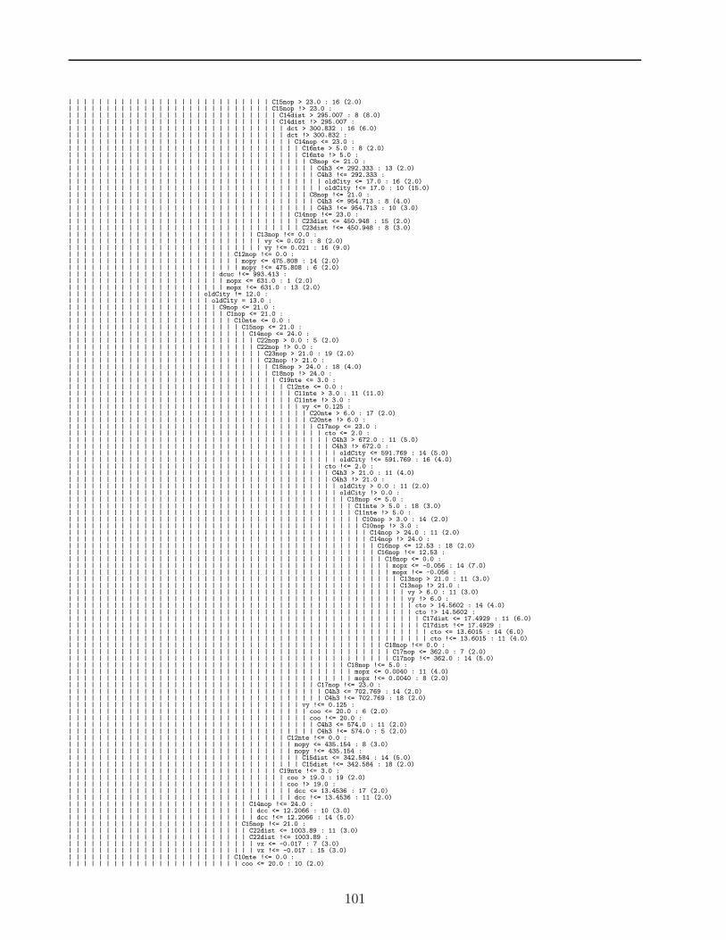
| | | | | | | | | | | | | | | | | | | | | | | | | | | C15nop > 23.0 : 16 (2.0)| | | | | | | | | | | | | | | | | | | | | | | | | | | C15nop !> 23.0 :| | | | | | | | | | | | | | | | | | | | | | | | | | | | C14dist > 295.007 : 8 (8.0)| | | | | | | | | | | | | | | | | | | | | | | | | | | | C14dist !> 295.007 :| | | | | | | | | | | | | | | | | | | | | | | | | | | | | dct > 300.832 : 16 (6.0)| | | | | | | | | | | | | | | | | | | | | | | | | | | | | dct !> 300.832 :| | | | | | | | | | | | | | | | | | | | | | | | | | | | | | C14nop <= 23.0 :| | | | | | | | | | | | | | | | | | | | | | | | | | | | | | | C16nte > 5.0 : 8 (2.0)| | | | | | | | | | | | | | | | | | | | | | | | | | | | | | | C16nte !> 5.0 :| | | | | | | | | | | | | | | | | | | | | | | | | | | | | | | | C8nop <= 21.0 :| | | | | | | | | | | | | | | | | | | | | | | | | | | | | | | | | C4h3 <= 292.333 : 13 (2.0)| | | | | | | | | | | | | | | | | | | | | | | | | | | | | | | | | C4h3 !<= 292.333 :| | | | | | | | | | | | | | | | | | | | | | | | | | | | | | | | | | oldCity <= 17.0 : 16 (2.0)| | | | | | | | | | | | | | | | | | | | | | | | | | | | | | | | | | oldCity !<= 17.0 : 10 (15.0)| | | | | | | | | | | | | | | | | | | | | | | | | | | | | | | | C8nop !<= 21.0 :| | | | | | | | | | | | | | | | | | | | | | | | | | | | | | | | | C4h3 <= 954.713 : 8 (4.0)| | | | | | | | | | | | | | | | | | | | | | | | | | | | | | | | | C4h3 !<= 954.713 : 10 (3.0)| | | | | | | | | | | | | | | | | | | | | | | | | | | | | | C14nop !<= 23.0 :| | | | | | | | | | | | | | | | | | | | | | | | | | | | | | | C23dist <= 450.948 : 15 (2.0)| | | | | | | | | | | | | | | | | | | | | | | | | | | | | | | C23dist !<= 450.948 : 8 (3.0)| | | | | | | | | | | | | | | | | | | | | | | | | C13nop !<= 0.0 :| | | | | | | | | | | | | | | | | | | | | | | | | | vy <= 0.021 : 8 (2.0)| | | | | | | | | | | | | | | | | | | | | | | | | | vy !<= 0.021 : 16 (9.0)| | | | | | | | | | | | | | | | | | | | | | C12nop !<= 0.0 :| | | | | | | | | | | | | | | | | | | | | | | mopy <= 475.808 : 14 (2.0)| | | | | | | | | | | | | | | | | | | | | | | mopy !<= 475.808 : 6 (2.0)| | | | | | | | | | | | | | | | | | | | dcuc !<= 993.413 :| | | | | | | | | | | | | | | | | | | | | mopx <= 631.0 : 1 (2.0)| | | | | | | | | | | | | | | | | | | | | mopx !<= 631.0 : 13 (2.0)| | | | | | | | | | | | | | | | | | oldCity != 12.0 :| | | | | | | | | | | | | | | | | | | oldCity = 13.0 :| | | | | | | | | | | | | | | | | | | | C9nop <= 21.0 :| | | | | | | | | | | | | | | | | | | | | C1nop <= 21.0 :| | | | | | | | | | | | | | | | | | | | | | C10nte <= 0.0 :| | | | | | | | | | | | | | | | | | | | | | | C15nop <= 21.0 :| | | | | | | | | | | | | | | | | | | | | | | | C14nop <= 24.0 :| | | | | | | | | | | | | | | | | | | | | | | | | C22nop > 0.0 : 5 (2.0)| | | | | | | | | | | | | | | | | | | | | | | | | C22nop !> 0.0 :| | | | | | | | | | | | | | | | | | | | | | | | | | C23nop > 21.0 : 19 (2.0)| | | | | | | | | | | | | | | | | | | | | | | | | | C23nop !> 21.0 :| | | | | | | | | | | | | | | | | | | | | | | | | | | C18nop > 24.0 : 18 (4.0)| | | | | | | | | | | | | | | | | | | | | | | | | | | C18nop !> 24.0 :| | | | | | | | | | | | | | | | | | | | | | | | | | | | C19nte <= 3.0 :| | | | | | | | | | | | | | | | | | | | | | | | | | | | | C12nte <= 0.0 :| | | | | | | | | | | | | | | | | | | | | | | | | | | | | | C11nte > 3.0 : 11 (11.0)| | | | | | | | | | | | | | | | | | | | | | | | | | | | | | C11nte !> 3.0 :| | | | | | | | | | | | | | | | | | | | | | | | | | | | | | | vy <= 0.125 :| | | | | | | | | | | | | | | | | | | | | | | | | | | | | | | | C20nte > 6.0 : 17 (2.0)| | | | | | | | | | | | | | | | | | | | | | | | | | | | | | | | C20nte !> 6.0 :| | | | | | | | | | | | | | | | | | | | | | | | | | | | | | | | | C17nop <= 23.0 :| | | | | | | | | | | | | | | | | | | | | | | | | | | | | | | | | | cto <= 2.0 :| | | | | | | | | | | | | | | | | | | | | | | | | | | | | | | | | | | C4h3 > 672.0 : 11 (5.0)| | | | | | | | | | | | | | | | | | | | | | | | | | | | | | | | | | | C4h3 !> 672.0 :| | | | | | | | | | | | | | | | | | | | | | | | | | | | | | | | | | | | oldCity <= 591.769 : 14 (5.0)| | | | | | | | | | | | | | | | | | | | | | | | | | | | | | | | | | | | oldCity !<= 591.769 : 16 (4.0)| | | | | | | | | | | | | | | | | | | | | | | | | | | | | | | | | | cto !<= 2.0 :| | | | | | | | | | | | | | | | | | | | | | | | | | | | | | | | | | | C4h3 > 21.0 : 11 (4.0)| | | | | | | | | | | | | | | | | | | | | | | | | | | | | | | | | | | C4h3 !> 21.0 :| | | | | | | | | | | | | | | | | | | | | | | | | | | | | | | | | | | | oldCity > 0.0 : 11 (2.0)| | | | | | | | | | | | | | | | | | | | | | | | | | | | | | | | | | | | oldCity !> 0.0 :| | | | | | | | | | | | | | | | | | | | | | | | | | | | | | | | | | | | | C18nop <= 5.0 :| | | | | | | | | | | | | | | | | | | | | | | | | | | | | | | | | | | | | | C11nte > 5.0 : 18 (3.0)| | | | | | | | | | | | | | | | | | | | | | | | | | | | | | | | | | | | | | C11nte !> 5.0 :| | | | | | | | | | | | | | | | | | | | | | | | | | | | | | | | | | | | | | | C10nop > 3.0 : 14 (2.0)| | | | | | | | | | | | | | | | | | | | | | | | | | | | | | | | | | | | | | | C10nop !> 3.0 :| | | | | | | | | | | | | | | | | | | | | | | | | | | | | | | | | | | | | | | | C14nop > 24.0 : 11 (2.0)| | | | | | | | | | | | | | | | | | | | | | | | | | | | | | | | | | | | | | | | C14nop !> 24.0 :| | | | | | | | | | | | | | | | | | | | | | | | | | | | | | | | | | | | | | | | | C16nop <= 12.53 : 18 (2.0)| | | | | | | | | | | | | | | | | | | | | | | | | | | | | | | | | | | | | | | | | C16nop !<= 12.53 :| | | | | | | | | | | | | | | | | | | | | | | | | | | | | | | | | | | | | | | | | | C18nop <= 0.0 :| | | | | | | | | | | | | | | | | | | | | | | | | | | | | | | | | | | | | | | | | | | mopx <= -0.056 : 14 (7.0)| | | | | | | | | | | | | | | | | | | | | | | | | | | | | | | | | | | | | | | | | | | mopx !<= -0.056 :| | | | | | | | | | | | | | | | | | | | | | | | | | | | | | | | | | | | | | | | | | | | C13nop > 21.0 : 11 (3.0)| | | | | | | | | | | | | | | | | | | | | | | | | | | | | | | | | | | | | | | | | | | | C13nop !> 21.0 :| | | | | | | | | | | | | | | | | | | | | | | | | | | | | | | | | | | | | | | | | | | | | vy > 6.0 : 11 (3.0)| | | | | | | | | | | | | | | | | | | | | | | | | | | | | | | | | | | | | | | | | | | | | vy !> 6.0 :| | | | | | | | | | | | | | | | | | | | | | | | | | | | | | | | | | | | | | | | | | | | | | cto > 14.5602 : 14 (4.0)| | | | | | | | | | | | | | | | | | | | | | | | | | | | | | | | | | | | | | | | | | | | | | cto !> 14.5602 :| | | | | | | | | | | | | | | | | | | | | | | | | | | | | | | | | | | | | | | | | | | | | | | C17dist <= 17.4929 : 11 (6.0)| | | | | | | | | | | | | | | | | | | | | | | | | | | | | | | | | | | | | | | | | | | | | | | C17dist !<= 17.4929 :| | | | | | | | | | | | | | | | | | | | | | | | | | | | | | | | | | | | | | | | | | | | | | | | cto <= 13.6015 : 14 (6.0)| | | | | | | | | | | | | | | | | | | | | | | | | | | | | | | | | | | | | | | | | | | | | | | | cto !<= 13.6015 : 11 (4.0)| | | | | | | | | | | | | | | | | | | | | | | | | | | | | | | | | | | | | | | | | | C18nop !<= 0.0 :| | | | | | | | | | | | | | | | | | | | | | | | | | | | | | | | | | | | | | | | | | | C17nop <= 362.0 : 7 (2.0)| | | | | | | | | | | | | | | | | | | | | | | | | | | | | | | | | | | | | | | | | | | C17nop !<= 362.0 : 14 (5.0)| | | | | | | | | | | | | | | | | | | | | | | | | | | | | | | | | | | | | C18nop !<= 5.0 :| | | | | | | | | | | | | | | | | | | | | | | | | | | | | | | | | | | | | | mopx <= 0.0040 : 11 (4.0)| | | | | | | | | | | | | | | | | | | | | | | | | | | | | | | | | | | | | | mopx !<= 0.0040 : 8 (2.0)| | | | | | | | | | | | | | | | | | | | | | | | | | | | | | | | | C17nop !<= 23.0 :| | | | | | | | | | | | | | | | | | | | | | | | | | | | | | | | | | C4h3 <= 702.769 : 14 (2.0)| | | | | | | | | | | | | | | | | | | | | | | | | | | | | | | | | | C4h3 !<= 702.769 : 18 (2.0)| | | | | | | | | | | | | | | | | | | | | | | | | | | | | | | vy !<= 0.125 :| | | | | | | | | | | | | | | | | | | | | | | | | | | | | | | | coo <= 20.0 : 6 (2.0)| | | | | | | | | | | | | | | | | | | | | | | | | | | | | | | | coo !<= 20.0 :| | | | | | | | | | | | | | | | | | | | | | | | | | | | | | | | | C4h3 <= 574.0 : 11 (2.0)| | | | | | | | | | | | | | | | | | | | | | | | | | | | | | | | | C4h3 !<= 574.0 : 5 (2.0)| | | | | | | | | | | | | | | | | | | | | | | | | | | | | C12nte !<= 0.0 :| | | | | | | | | | | | | | | | | | | | | | | | | | | | | | mopy <= 435.154 : 8 (3.0)| | | | | | | | | | | | | | | | | | | | | | | | | | | | | | mopy !<= 435.154 :| | | | | | | | | | | | | | | | | | | | | | | | | | | | | | | C15dist <= 342.584 : 14 (5.0)| | | | | | | | | | | | | | | | | | | | | | | | | | | | | | | C15dist !<= 342.584 : 18 (2.0)| | | | | | | | | | | | | | | | | | | | | | | | | | | | C19nte !<= 3.0 :| | | | | | | | | | | | | | | | | | | | | | | | | | | | | coo > 19.0 : 19 (2.0)| | | | | | | | | | | | | | | | | | | | | | | | | | | | | coo !> 19.0 :| | | | | | | | | | | | | | | | | | | | | | | | | | | | | | dcc <= 13.4536 : 17 (2.0)| | | | | | | | | | | | | | | | | | | | | | | | | | | | | | dcc !<= 13.4536 : 11 (2.0)| | | | | | | | | | | | | | | | | | | | | | | | C14nop !<= 24.0 :| | | | | | | | | | | | | | | | | | | | | | | | | dcc <= 12.2066 : 10 (3.0)| | | | | | | | | | | | | | | | | | | | | | | | | dcc !<= 12.2066 : 14 (5.0)| | | | | | | | | | | | | | | | | | | | | | | C15nop !<= 21.0 :| | | | | | | | | | | | | | | | | | | | | | | | C22dist <= 1003.89 : 11 (3.0)| | | | | | | | | | | | | | | | | | | | | | | | C22dist !<= 1003.89 :| | | | | | | | | | | | | | | | | | | | | | | | | vx <= -0.017 : 7 (3.0)| | | | | | | | | | | | | | | | | | | | | | | | | vx !<= -0.017 : 15 (3.0)| | | | | | | | | | | | | | | | | | | | | | C10nte !<= 0.0 :| | | | | | | | | | | | | | | | | | | | | | | coo <= 20.0 : 10 (2.0)
101

| | | | | | | | | | | | | | | | | | | | | | | coo !<= 20.0 : 14 (2.0)| | | | | | | | | | | | | | | | | | | | | C1nop !<= 21.0 :| | | | | | | | | | | | | | | | | | | | | | C1nop <= 23.0 : 18 (3.0)| | | | | | | | | | | | | | | | | | | | | | C1nop !<= 23.0 : 4 (2.0)| | | | | | | | | | | | | | | | | | | | C9nop !<= 21.0 :| | | | | | | | | | | | | | | | | | | | | ply <= 891.0 : 12 (2.0)| | | | | | | | | | | | | | | | | | | | | ply !<= 891.0 : 3 (3.0)| | | | | | | | | | | | | | | | | | | oldCity != 13.0 :| | | | | | | | | | | | | | | | | | | | oldCity = 14.0 :| | | | | | | | | | | | | | | | | | | | | plx <= 1021.0 :| | | | | | | | | | | | | | | | | | | | | | C10nop <= 21.0 :| | | | | | | | | | | | | | | | | | | | | | | C17nte <= 3.0 :| | | | | | | | | | | | | | | | | | | | | | | | C23nop <= 0.0 :| | | | | | | | | | | | | | | | | | | | | | | | | C15nte <= 0.0 :| | | | | | | | | | | | | | | | | | | | | | | | | | C7nop <= 23.0 :| | | | | | | | | | | | | | | | | | | | | | | | | | | C12nop <= 23.0 :| | | | | | | | | | | | | | | | | | | | | | | | | | | | C14nop <= 24.0 :| | | | | | | | | | | | | | | | | | | | | | | | | | | | | C11nte <= 0.0 :| | | | | | | | | | | | | | | | | | | | | | | | | | | | | | C19nop <= 23.0 :| | | | | | | | | | | | | | | | | | | | | | | | | | | | | | | C1nop > 23.0 : 16 (3.0)| | | | | | | | | | | | | | | | | | | | | | | | | | | | | | | C1nop !> 23.0 :| | | | | | | | | | | | | | | | | | | | | | | | | | | | | | | | C19nte > 6.0 : 13 (2.0)| | | | | | | | | | | | | | | | | | | | | | | | | | | | | | | | C19nte !> 6.0 :| | | | | | | | | | | | | | | | | | | | | | | | | | | | | | | | | C2nop > 0.0 : 13 (2.0)| | | | | | | | | | | | | | | | | | | | | | | | | | | | | | | | | C2nop !> 0.0 :| | | | | | | | | | | | | | | | | | | | | | | | | | | | | | | | | | C4h3 > 23.0 : 17 (2.0)| | | | | | | | | | | | | | | | | | | | | | | | | | | | | | | | | | C4h3 !> 23.0 :| | | | | | | | | | | | | | | | | | | | | | | | | | | | | | | | | | | oldCity <= 3.0 :| | | | | | | | | | | | | | | | | | | | | | | | | | | | | | | | | | | | C18nop <= 0.0 :| | | | | | | | | | | | | | | | | | | | | | | | | | | | | | | | | | | | | C11nte > 21.0 : 16 (3.0)| | | | | | | | | | | | | | | | | | | | | | | | | | | | | | | | | | | | | C11nte !> 21.0 :| | | | | | | | | | | | | | | | | | | | | | | | | | | | | | | | | | | | | | C10nop <= 522.462 :| | | | | | | | | | | | | | | | | | | | | | | | | | | | | | | | | | | | | | | oldCity <= 0.0 :| | | | | | | | | | | | | | | | | | | | | | | | | | | | | | | | | | | | | | | | C14nop > 0.0 : 16 (2.0)| | | | | | | | | | | | | | | | | | | | | | | | | | | | | | | | | | | | | | | | C14nop !> 0.0 :| | | | | | | | | | | | | | | | | | | | | | | | | | | | | | | | | | | | | | | | | C16nop > 0.0 : 16 (2.0)| | | | | | | | | | | | | | | | | | | | | | | | | | | | | | | | | | | | | | | | | C16nop !> 0.0 :| | | | | | | | | | | | | | | | | | | | | | | | | | | | | | | | | | | | | | | | | | mopx <= 0.0 :| | | | | | | | | | | | | | | | | | | | | | | | | | | | | | | | | | | | | | | | | | | C13nop <= 3.0 :| | | | | | | | | | | | | | | | | | | | | | | | | | | | | | | | | | | | | | | | | | | | vy <= 13.6015 : 13 (4.0)| | | | | | | | | | | | | | | | | | | | | | | | | | | | | | | | | | | | | | | | | | | | vy !<= 13.6015 :| | | | | | | | | | | | | | | | | | | | | | | | | | | | | | | | | | | | | | | | | | | | | cto <= 6.0 :| | | | | | | | | | | | | | | | | | | | | | | | | | | | | | | | | | | | | | | | | | | | | | C17dist > 347.96 : 13 (5.0)| | | | | | | | | | | | | | | | | | | | | | | | | | | | | | | | | | | | | | | | | | | | | | C17dist !> 347.96 :| | | | | | | | | | | | | | | | | | | | | | | | | | | | | | | | | | | | | | | | | | | | | | | C17nop <= 0.0010 : 16 (29.0)| | | | | | | | | | | | | | | | | | | | | | | | | | | | | | | | | | | | | | | | | | | | | | | C17nop !<= 0.0010 :| | | | | | | | | | | | | | | | | | | | | | | | | | | | | | | | | | | | | | | | | | | | | | | | C24nop <= 14.1421 : 13 (6.0)| | | | | | | | | | | | | | | | | | | | | | | | | | | | | | | | | | | | | | | | | | | | | | | | C24nop !<= 14.1421 :| | | | | | | | | | | | | | | | | | | | | | | | | | | | | | | | | | | | | | | | | | | | | | | | | C11dist <= 9.0 : 16 (4.0)| | | | | | | | | | | | | | | | | | | | | | | | | | | | | | | | | | | | | | | | | | | | | | | | | C11dist !<= 9.0 : 13 (3.0)| | | | | | | | | | | | | | | | | | | | | | | | | | | | | | | | | | | | | | | | | | | | | cto !<= 6.0 :| | | | | | | | | | | | | | | | | | | | | | | | | | | | | | | | | | | | | | | | | | | | | | C17nop > -0.017 : 13 (4.0)| | | | | | | | | | | | | | | | | | | | | | | | | | | | | | | | | | | | | | | | | | | | | | C17nop !> -0.017 :| | | | | | | | | | | | | | | | | | | | | | | | | | | | | | | | | | | | | | | | | | | | | | | C10nop <= 429.577 : 16 (2.0)| | | | | | | | | | | | | | | | | | | | | | | | | | | | | | | | | | | | | | | | | | | | | | | C10nop !<= 429.577 : 11 (2.0)| | | | | | | | | | | | | | | | | | | | | | | | | | | | | | | | | | | | | | | | | | | C13nop !<= 3.0 :| | | | | | | | | | | | | | | | | | | | | | | | | | | | | | | | | | | | | | | | | | | | C11dist <= 6.0 : 18 (3.0)| | | | | | | | | | | | | | | | | | | | | | | | | | | | | | | | | | | | | | | | | | | | C11dist !<= 6.0 :| | | | | | | | | | | | | | | | | | | | | | | | | | | | | | | | | | | | | | | | | | | | | C17dist <= 33.2866 : 11 (2.0)| | | | | | | | | | | | | | | | | | | | | | | | | | | | | | | | | | | | | | | | | | | | | C17dist !<= 33.2866 : 16 (5.0)| | | | | | | | | | | | | | | | | | | | | | | | | | | | | | | | | | | | | | | | | | mopx !<= 0.0 :| | | | | | | | | | | | | | | | | | | | | | | | | | | | | | | | | | | | | | | | | | | C8nte <= 473.25 : 13 (3.0)| | | | | | | | | | | | | | | | | | | | | | | | | | | | | | | | | | | | | | | | | | | C8nte !<= 473.25 : 16 (4.0)| | | | | | | | | | | | | | | | | | | | | | | | | | | | | | | | | | | | | | | oldCity !<= 0.0 :| | | | | | | | | | | | | | | | | | | | | | | | | | | | | | | | | | | | | | | | C15nte <= 571.008 : 16 (3.0)| | | | | | | | | | | | | | | | | | | | | | | | | | | | | | | | | | | | | | | | C15nte !<= 571.008 : 13 (3.0)| | | | | | | | | | | | | | | | | | | | | | | | | | | | | | | | | | | | | | C10nop !<= 522.462 :| | | | | | | | | | | | | | | | | | | | | | | | | | | | | | | | | | | | | | | C17dist <= 117.209 : 18 (5.0)| | | | | | | | | | | | | | | | | | | | | | | | | | | | | | | | | | | | | | | C17dist !<= 117.209 :| | | | | | | | | | | | | | | | | | | | | | | | | | | | | | | | | | | | | | | | C16nte <= 15.0 : 8 (2.0)| | | | | | | | | | | | | | | | | | | | | | | | | | | | | | | | | | | | | | | | C16nte !<= 15.0 : 13 (9.0)| | | | | | | | | | | | | | | | | | | | | | | | | | | | | | | | | | | | C18nop !<= 0.0 :| | | | | | | | | | | | | | | | | | | | | | | | | | | | | | | | | | | | | mtpx <= 555.739 : 18 (3.0)| | | | | | | | | | | | | | | | | | | | | | | | | | | | | | | | | | | | | mtpx !<= 555.739 : 13 (3.0)| | | | | | | | | | | | | | | | | | | | | | | | | | | | | | | | | | | oldCity !<= 3.0 :| | | | | | | | | | | | | | | | | | | | | | | | | | | | | | | | | | | | mtpx > 667.381 : 17 (2.0)| | | | | | | | | | | | | | | | | | | | | | | | | | | | | | | | | | | | mtpx !> 667.381 :| | | | | | | | | | | | | | | | | | | | | | | | | | | | | | | | | | | | | C12nop > 21.0 : 18 (3.0)| | | | | | | | | | | | | | | | | | | | | | | | | | | | | | | | | | | | | C12nop !> 21.0 :| | | | | | | | | | | | | | | | | | | | | | | | | | | | | | | | | | | | | | mtpx <= 562.261 : 13 (2.0)| | | | | | | | | | | | | | | | | | | | | | | | | | | | | | | | | | | | | | mtpx !<= 562.261 : 18 (2.0)| | | | | | | | | | | | | | | | | | | | | | | | | | | | | | C19nop !<= 23.0 :| | | | | | | | | | | | | | | | | | | | | | | | | | | | | | | mopx <= 677.731 : 8 (2.0)| | | | | | | | | | | | | | | | | | | | | | | | | | | | | | | mopx !<= 677.731 : 9 (2.0)| | | | | | | | | | | | | | | | | | | | | | | | | | | | | C11nte !<= 0.0 :| | | | | | | | | | | | | | | | | | | | | | | | | | | | | | dcuc <= 14.2127 :| | | | | | | | | | | | | | | | | | | | | | | | | | | | | | | cto <= 6.0 : 9 (2.0)| | | | | | | | | | | | | | | | | | | | | | | | | | | | | | | cto !<= 6.0 : 11 (2.0)| | | | | | | | | | | | | | | | | | | | | | | | | | | | | | dcuc !<= 14.2127 :| | | | | | | | | | | | | | | | | | | | | | | | | | | | | | | cto <= 2.0 : 11 (3.0)| | | | | | | | | | | | | | | | | | | | | | | | | | | | | | | cto !<= 2.0 :| | | | | | | | | | | | | | | | | | | | | | | | | | | | | | | | C11nop > 24.0 : 18 (4.0)| | | | | | | | | | | | | | | | | | | | | | | | | | | | | | | | C11nop !> 24.0 :| | | | | | | | | | | | | | | | | | | | | | | | | | | | | | | | | dcc <= 14.4222 : 18 (4.0)| | | | | | | | | | | | | | | | | | | | | | | | | | | | | | | | | dcc !<= 14.4222 : 16 (2.0)| | | | | | | | | | | | | | | | | | | | | | | | | | | | C14nop !<= 24.0 :| | | | | | | | | | | | | | | | | | | | | | | | | | | | | cto <= 6.0 : 16 (2.0)| | | | | | | | | | | | | | | | | | | | | | | | | | | | | cto !<= 6.0 :| | | | | | | | | | | | | | | | | | | | | | | | | | | | | | mopx <= 708.038 : 7 (3.0)| | | | | | | | | | | | | | | | | | | | | | | | | | | | | | mopx !<= 708.038 : 13 (3.0)| | | | | | | | | | | | | | | | | | | | | | | | | | | C12nop !<= 23.0 :| | | | | | | | | | | | | | | | | | | | | | | | | | | | dcc <= 14.0357 : 8 (4.0)| | | | | | | | | | | | | | | | | | | | | | | | | | | | dcc !<= 14.0357 : 16 (2.0)| | | | | | | | | | | | | | | | | | | | | | | | | | C7nop !<= 23.0 :| | | | | | | | | | | | | | | | | | | | | | | | | | | mopx <= 639.5 : 7 (2.0)| | | | | | | | | | | | | | | | | | | | | | | | | | | mopx !<= 639.5 : 15 (2.0)| | | | | | | | | | | | | | | | | | | | | | | | | C15nte !<= 0.0 :| | | | | | | | | | | | | | | | | | | | | | | | | | dcc <= 12.2066 :| | | | | | | | | | | | | | | | | | | | | | | | | | | mtpy <= 341.6 : 15 (2.0)| | | | | | | | | | | | | | | | | | | | | | | | | | | mtpy !<= 341.6 : 8 (2.0)| | | | | | | | | | | | | | | | | | | | | | | | | | dcc !<= 12.2066 :| | | | | | | | | | | | | | | | | | | | | | | | | | | mopx <= 643.269 : 11 (2.0)| | | | | | | | | | | | | | | | | | | | | | | | | | | mopx !<= 643.269 : 20 (2.0)| | | | | | | | | | | | | | | | | | | | | | | | C23nop !<= 0.0 :| | | | | | | | | | | | | | | | | | | | | | | | | C20dist <= 255.947 : 20 (2.0)| | | | | | | | | | | | | | | | | | | | | | | | | C20dist !<= 255.947 : 12 (3.0)
102

| | | | | | | | | | | | | | | | | | | | | | | C17nte !<= 3.0 :| | | | | | | | | | | | | | | | | | | | | | | | C24dist <= 438.926 : 18 (2.0)| | | | | | | | | | | | | | | | | | | | | | | | C24dist !<= 438.926 : 5 (3.0)| | | | | | | | | | | | | | | | | | | | | | C10nop !<= 21.0 :| | | | | | | | | | | | | | | | | | | | | | | mopx <= 572.87 : 7 (2.0)| | | | | | | | | | | | | | | | | | | | | | | mopx !<= 572.87 : 17 (2.0)| | | | | | | | | | | | | | | | | | | | | plx !<= 1021.0 :| | | | | | | | | | | | | | | | | | | | | | C5nop > 0.0 : 3 (2.0)| | | | | | | | | | | | | | | | | | | | | | C5nop !> 0.0 :| | | | | | | | | | | | | | | | | | | | | | | C3nte > 3.0 : 10 (3.0)| | | | | | | | | | | | | | | | | | | | | | | C3nte !> 3.0 :| | | | | | | | | | | | | | | | | | | | | | | | coo <= 17.0 : 17 (2.0)| | | | | | | | | | | | | | | | | | | | | | | | coo !<= 17.0 : 1 (3.0)| | | | | | | | | | | | | | | | | | | | oldCity != 14.0 :| | | | | | | | | | | | | | | | | | | | | oldCity = 15.0 :| | | | | | | | | | | | | | | | | | | | | | C18nte <= 3.0 :| | | | | | | | | | | | | | | | | | | | | | | C16nte <= 0.0 :| | | | | | | | | | | | | | | | | | | | | | | | C6nop <= 0.0 :| | | | | | | | | | | | | | | | | | | | | | | | | C11nop <= 21.0 :| | | | | | | | | | | | | | | | | | | | | | | | | | C17nop <= 24.0 :| | | | | | | | | | | | | | | | | | | | | | | | | | | dct <= 9.05539 :| | | | | | | | | | | | | | | | | | | | | | | | | | | | C8nop <= 0.0 : 11 (4.0)| | | | | | | | | | | | | | | | | | | | | | | | | | | | C8nop !<= 0.0 : 12 (3.0)| | | | | | | | | | | | | | | | | | | | | | | | | | | dct !<= 9.05539 :| | | | | | | | | | | | | | | | | | | | | | | | | | | | C14nop <= 23.0 :| | | | | | | | | | | | | | | | | | | | | | | | | | | | | mopy <= 540.043 :| | | | | | | | | | | | | | | | | | | | | | | | | | | | | | C2nop > 0.0 : 7 (2.0)| | | | | | | | | | | | | | | | | | | | | | | | | | | | | | C2nop !> 0.0 :| | | | | | | | | | | | | | | | | | | | | | | | | | | | | | | C11nte > 3.0 : 8 (3.0)| | | | | | | | | | | | | | | | | | | | | | | | | | | | | | | C11nte !> 3.0 :| | | | | | | | | | | | | | | | | | | | | | | | | | | | | | | | C13dist <= 13.4536 : 7 (6.0)| | | | | | | | | | | | | | | | | | | | | | | | | | | | | | | | C13dist !<= 13.4536 :| | | | | | | | | | | | | | | | | | | | | | | | | | | | | | | | | mopx <= 659.333 :| | | | | | | | | | | | | | | | | | | | | | | | | | | | | | | | | | C8nop > 21.0 : 7 (2.0)| | | | | | | | | | | | | | | | | | | | | | | | | | | | | | | | | | C8nop !> 21.0 :| | | | | | | | | | | | | | | | | | | | | | | | | | | | | | | | | | | plx <= 33.0 : 7 (2.0)| | | | | | | | | | | | | | | | | | | | | | | | | | | | | | | | | | | plx !<= 33.0 :| | | | | | | | | | | | | | | | | | | | | | | | | | | | | | | | | | | | C4h3 <= 15.0 : 7 (3.0)| | | | | | | | | | | | | | | | | | | | | | | | | | | | | | | | | | | | C4h3 !<= 15.0 :| | | | | | | | | | | | | | | | | | | | | | | | | | | | | | | | | | | | | oldCity <= 302.552 : 7 (3.0)| | | | | | | | | | | | | | | | | | | | | | | | | | | | | | | | | | | | | oldCity !<= 302.552 :| | | | | | | | | | | | | | | | | | | | | | | | | | | | | | | | | | | | | | C18nop <= 356.679 : 8 (19.0)| | | | | | | | | | | | | | | | | | | | | | | | | | | | | | | | | | | | | | C18nop !<= 356.679 :| | | | | | | | | | | | | | | | | | | | | | | | | | | | | | | | | | | | | | | C11nte <= 570.909 : 8 (7.0)| | | | | | | | | | | | | | | | | | | | | | | | | | | | | | | | | | | | | | | C11nte !<= 570.909 : 7 (5.0)| | | | | | | | | | | | | | | | | | | | | | | | | | | | | | | | | mopx !<= 659.333 :| | | | | | | | | | | | | | | | | | | | | | | | | | | | | | | | | | dco <= 89.2749 :| | | | | | | | | | | | | | | | | | | | | | | | | | | | | | | | | | | C4h3 <= 512.191 : 7 (3.0)| | | | | | | | | | | | | | | | | | | | | | | | | | | | | | | | | | | C4h3 !<= 512.191 : 8 (7.0)| | | | | | | | | | | | | | | | | | | | | | | | | | | | | | | | | | dco !<= 89.2749 :| | | | | | | | | | | | | | | | | | | | | | | | | | | | | | | | | | | vx > 0.011 : 6 (5.0)| | | | | | | | | | | | | | | | | | | | | | | | | | | | | | | | | | | vx !> 0.011 :| | | | | | | | | | | | | | | | | | | | | | | | | | | | | | | | | | | | C4h3 <= 484.423 : 12 (4.0)| | | | | | | | | | | | | | | | | | | | | | | | | | | | | | | | | | | | C4h3 !<= 484.423 :| | | | | | | | | | | | | | | | | | | | | | | | | | | | | | | | | | | | | oldCity <= 307.875 : 6 (2.0)| | | | | | | | | | | | | | | | | | | | | | | | | | | | | | | | | | | | | oldCity !<= 307.875 : 8 (2.0)| | | | | | | | | | | | | | | | | | | | | | | | | | | | | mopy !<= 540.043 :| | | | | | | | | | | | | | | | | | | | | | | | | | | | | | C12dist <= 393.406 :| | | | | | | | | | | | | | | | | | | | | | | | | | | | | | | dcc <= 14.0357 : 14 (3.0)| | | | | | | | | | | | | | | | | | | | | | | | | | | | | | | dcc !<= 14.0357 :| | | | | | | | | | | | | | | | | | | | | | | | | | | | | | | | mtpx <= 453.667 : 11 (2.0)| | | | | | | | | | | | | | | | | | | | | | | | | | | | | | | | mtpx !<= 453.667 : 8 (2.0)| | | | | | | | | | | | | | | | | | | | | | | | | | | | | | C12dist !<= 393.406 :| | | | | | | | | | | | | | | | | | | | | | | | | | | | | | | vy <= 0.038 : 6 (3.0)| | | | | | | | | | | | | | | | | | | | | | | | | | | | | | | vy !<= 0.038 : 9 (2.0)| | | | | | | | | | | | | | | | | | | | | | | | | | | | C14nop !<= 23.0 :| | | | | | | | | | | | | | | | | | | | | | | | | | | | | C14nop <= 24.0 : 6 (3.0)| | | | | | | | | | | | | | | | | | | | | | | | | | | | | C14nop !<= 24.0 :| | | | | | | | | | | | | | | | | | | | | | | | | | | | | | dcc <= 14.1421 : 12 (2.0)| | | | | | | | | | | | | | | | | | | | | | | | | | | | | | dcc !<= 14.1421 : 7 (3.0)| | | | | | | | | | | | | | | | | | | | | | | | | | C17nop !<= 24.0 :| | | | | | | | | | | | | | | | | | | | | | | | | | | mtpx <= 417.0 : 13 (3.0)| | | | | | | | | | | | | | | | | | | | | | | | | | | mtpx !<= 417.0 : 7 (2.0)| | | | | | | | | | | | | | | | | | | | | | | | | C11nop !<= 21.0 :| | | | | | | | | | | | | | | | | | | | | | | | | | C11dist <= 12.7279 : 6 (2.0)| | | | | | | | | | | | | | | | | | | | | | | | | | C11dist !<= 12.7279 :| | | | | | | | | | | | | | | | | | | | | | | | | | | vx <= 0.021 : 13 (3.0)| | | | | | | | | | | | | | | | | | | | | | | | | | | vx !<= 0.021 : 8 (2.0)| | | | | | | | | | | | | | | | | | | | | | | | C6nop !<= 0.0 :| | | | | | | | | | | | | | | | | | | | | | | | | C24dist <= 1173.69 : 8 (2.0)| | | | | | | | | | | | | | | | | | | | | | | | | C24dist !<= 1173.69 : 6 (3.0)| | | | | | | | | | | | | | | | | | | | | | | C16nte !<= 0.0 :| | | | | | | | | | | | | | | | | | | | | | | | mtpy <= 419.0 : 16 (3.0)| | | | | | | | | | | | | | | | | | | | | | | | mtpy !<= 419.0 :| | | | | | | | | | | | | | | | | | | | | | | | | mopy <= 501.577 : 8 (2.0)| | | | | | | | | | | | | | | | | | | | | | | | | mopy !<= 501.577 : 7 (2.0)| | | | | | | | | | | | | | | | | | | | | | C18nte !<= 3.0 :| | | | | | | | | | | | | | | | | | | | | | | dco <= 52.3927 : 18 (3.0)| | | | | | | | | | | | | | | | | | | | | | | dco !<= 52.3927 : 19 (2.0)| | | | | | | | | | | | | | | | | | | | | oldCity != 15.0 :| | | | | | | | | | | | | | | | | | | | | | oldCity = 16.0 :| | | | | | | | | | | | | | | | | | | | | | | C1nte <= 0.0 :| | | | | | | | | | | | | | | | | | | | | | | | C17nop > 23.0 : 6 (2.0)| | | | | | | | | | | | | | | | | | | | | | | | C17nop !> 23.0 :| | | | | | | | | | | | | | | | | | | | | | | | | vx <= 0.154 :| | | | | | | | | | | | | | | | | | | | | | | | | | C2nop > 0.0 : 12 (2.0)| | | | | | | | | | | | | | | | | | | | | | | | | | C2nop !> 0.0 :| | | | | | | | | | | | | | | | | | | | | | | | | | | C6nop > 0.0 : 8 (2.0)| | | | | | | | | | | | | | | | | | | | | | | | | | | C6nop !> 0.0 :| | | | | | | | | | | | | | | | | | | | | | | | | | | | C12nop <= 21.0 :| | | | | | | | | | | | | | | | | | | | | | | | | | | | | C8nop <= 0.0 :| | | | | | | | | | | | | | | | | | | | | | | | | | | | | | C7nte <= 0.0 :| | | | | | | | | | | | | | | | | | | | | | | | | | | | | | | C12nte > 3.0 : 14 (3.0)| | | | | | | | | | | | | | | | | | | | | | | | | | | | | | | C12nte !> 3.0 :| | | | | | | | | | | | | | | | | | | | | | | | | | | | | | | | C16dist <= 12.3693 : 8 (2.0)| | | | | | | | | | | | | | | | | | | | | | | | | | | | | | | | C16dist !<= 12.3693 :| | | | | | | | | | | | | | | | | | | | | | | | | | | | | | | | | C11nte <= 5.0 :| | | | | | | | | | | | | | | | | | | | | | | | | | | | | | | | | | C10nte > 5.0 : 12 (2.0)| | | | | | | | | | | | | | | | | | | | | | | | | | | | | | | | | | C10nte !> 5.0 :| | | | | | | | | | | | | | | | | | | | | | | | | | | | | | | | | | | C14nte > 3.0 : 14 (9.0)| | | | | | | | | | | | | | | | | | | | | | | | | | | | | | | | | | | C14nte !> 3.0 :| | | | | | | | | | | | | | | | | | | | | | | | | | | | | | | | | | | | C4h3 > 0.0 : 13 (2.0)| | | | | | | | | | | | | | | | | | | | | | | | | | | | | | | | | | | | C4h3 !> 0.0 :| | | | | | | | | | | | | | | | | | | | | | | | | | | | | | | | | | | | | oldCity <= 19.4165 : 13 (2.0)| | | | | | | | | | | | | | | | | | | | | | | | | | | | | | | | | | | | | oldCity !<= 19.4165 :| | | | | | | | | | | | | | | | | | | | | | | | | | | | | | | | | | | | | | C18nop > 0.0 : 14 (6.0)
103

| | | | | | | | | | | | | | | | | | | | | | | | | | | | | | | | | | | | | | C18nop !> 0.0 :| | | | | | | | | | | | | | | | | | | | | | | | | | | | | | | | | | | | | | | C11nte <= 13.0 :| | | | | | | | | | | | | | | | | | | | | | | | | | | | | | | | | | | | | | | | C10nop <= 197.709 : 11 (3.0)| | | | | | | | | | | | | | | | | | | | | | | | | | | | | | | | | | | | | | | | C10nop !<= 197.709 : 14 (10.0)| | | | | | | | | | | | | | | | | | | | | | | | | | | | | | | | | | | | | | | C11nte !<= 13.0 :| | | | | | | | | | | | | | | | | | | | | | | | | | | | | | | | | | | | | | | | C14nop <= 0.0 :| | | | | | | | | | | | | | | | | | | | | | | | | | | | | | | | | | | | | | | | | C16nop > 18.0 : 14 (25.0)| | | | | | | | | | | | | | | | | | | | | | | | | | | | | | | | | | | | | | | | | C16nop !> 18.0 :| | | | | | | | | | | | | | | | | | | | | | | | | | | | | | | | | | | | | | | | | | C11nte <= 14.2127 : 12 (7.0)| | | | | | | | | | | | | | | | | | | | | | | | | | | | | | | | | | | | | | | | | | C11nte !<= 14.2127 :| | | | | | | | | | | | | | | | | | | | | | | | | | | | | | | | | | | | | | | | | | | mopx <= 628.304 : 12 (2.0)| | | | | | | | | | | | | | | | | | | | | | | | | | | | | | | | | | | | | | | | | | | mopx !<= 628.304 : 14 (7.0)| | | | | | | | | | | | | | | | | | | | | | | | | | | | | | | | | | | | | | | | C14nop !<= 0.0 :| | | | | | | | | | | | | | | | | | | | | | | | | | | | | | | | | | | | | | | | | C13nop > 369.333 : 13 (2.0)| | | | | | | | | | | | | | | | | | | | | | | | | | | | | | | | | | | | | | | | | C13nop !> 369.333 :| | | | | | | | | | | | | | | | | | | | | | | | | | | | | | | | | | | | | | | | | | vy <= 101.203 : 14 (9.0)| | | | | | | | | | | | | | | | | | | | | | | | | | | | | | | | | | | | | | | | | | vy !<= 101.203 : 12 (3.0)| | | | | | | | | | | | | | | | | | | | | | | | | | | | | | | | | C11nte !<= 5.0 :| | | | | | | | | | | | | | | | | | | | | | | | | | | | | | | | | | mopx <= 526.231 : 14 (4.0)| | | | | | | | | | | | | | | | | | | | | | | | | | | | | | | | | | mopx !<= 526.231 : 18 (2.0)| | | | | | | | | | | | | | | | | | | | | | | | | | | | | | C7nte !<= 0.0 :| | | | | | | | | | | | | | | | | | | | | | | | | | | | | | | dcc <= 14.1421 : 13 (3.0)| | | | | | | | | | | | | | | | | | | | | | | | | | | | | | | dcc !<= 14.1421 : 14 (2.0)| | | | | | | | | | | | | | | | | | | | | | | | | | | | | C8nop !<= 0.0 :| | | | | | | | | | | | | | | | | | | | | | | | | | | | | | dct > 208.082 : 12 (5.0)| | | | | | | | | | | | | | | | | | | | | | | | | | | | | | dct !> 208.082 :| | | | | | | | | | | | | | | | | | | | | | | | | | | | | | | C24dist <= 986.071 : 10 (2.0)| | | | | | | | | | | | | | | | | | | | | | | | | | | | | | | C24dist !<= 986.071 : 8 (3.0)| | | | | | | | | | | | | | | | | | | | | | | | | | | | C12nop !<= 21.0 :| | | | | | | | | | | | | | | | | | | | | | | | | | | | | C12nop <= 24.0 : 10 (2.0)| | | | | | | | | | | | | | | | | | | | | | | | | | | | | C12nop !<= 24.0 : 14 (4.0)| | | | | | | | | | | | | | | | | | | | | | | | | vx !<= 0.154 :| | | | | | | | | | | | | | | | | | | | | | | | | | mopx <= 664.333 : 18 (2.0)| | | | | | | | | | | | | | | | | | | | | | | | | | mopx !<= 664.333 : 17 (2.0)| | | | | | | | | | | | | | | | | | | | | | | C1nte !<= 0.0 :| | | | | | | | | | | | | | | | | | | | | | | | mopy <= 445.609 : 1 (2.0)| | | | | | | | | | | | | | | | | | | | | | | | mopy !<= 445.609 : 14 (2.0)| | | | | | | | | | | | | | | | | | | | | | oldCity != 16.0 :| | | | | | | | | | | | | | | | | | | | | | | oldCity = 17.0 :| | | | | | | | | | | | | | | | | | | | | | | | C15nte <= 0.0 :| | | | | | | | | | | | | | | | | | | | | | | | | C12nte <= 0.0 :| | | | | | | | | | | | | | | | | | | | | | | | | | C8nte <= 3.0 :| | | | | | | | | | | | | | | | | | | | | | | | | | | dcuc <= 666.325 :| | | | | | | | | | | | | | | | | | | | | | | | | | | | C17nop <= 23.0 :| | | | | | | | | | | | | | | | | | | | | | | | | | | | | C2nop > 0.0 : 2 (3.0)| | | | | | | | | | | | | | | | | | | | | | | | | | | | | C2nop !> 0.0 :| | | | | | | | | | | | | | | | | | | | | | | | | | | | | | C9nop <= 23.0 :| | | | | | | | | | | | | | | | | | | | | | | | | | | | | | | vy <= -0.148 :| | | | | | | | | | | | | | | | | | | | | | | | | | | | | | | | C8dist <= 409.941 :| | | | | | | | | | | | | | | | | | | | | | | | | | | | | | | | | vy <= -0.153 : 19 (8.0)| | | | | | | | | | | | | | | | | | | | | | | | | | | | | | | | | vy !<= -0.153 : 18 (2.0)| | | | | | | | | | | | | | | | | | | | | | | | | | | | | | | | C8dist !<= 409.941 :| | | | | | | | | | | | | | | | | | | | | | | | | | | | | | | | | mopx <= 574.417 : 14 (2.0)| | | | | | | | | | | | | | | | | | | | | | | | | | | | | | | | | mopx !<= 574.417 : 7 (2.0)| | | | | | | | | | | | | | | | | | | | | | | | | | | | | | | vy !<= -0.148 :| | | | | | | | | | | | | | | | | | | | | | | | | | | | | | | | C14nop > 24.0 : 8 (3.0)| | | | | | | | | | | | | | | | | | | | | | | | | | | | | | | | C14nop !> 24.0 :| | | | | | | | | | | | | | | | | | | | | | | | | | | | | | | | | ply <= 335.0 :| | | | | | | | | | | | | | | | | | | | | | | | | | | | | | | | | | C5dist <= 858.242 :| | | | | | | | | | | | | | | | | | | | | | | | | | | | | | | | | | | mopy <= 438.792 : 11 (2.0)| | | | | | | | | | | | | | | | | | | | | | | | | | | | | | | | | | | mopy !<= 438.792 : 20 (2.0)| | | | | | | | | | | | | | | | | | | | | | | | | | | | | | | | | | C5dist !<= 858.242 :| | | | | | | | | | | | | | | | | | | | | | | | | | | | | | | | | | | dco <= 130.138 : 9 (3.0)| | | | | | | | | | | | | | | | | | | | | | | | | | | | | | | | | | | dco !<= 130.138 : 16 (2.0)| | | | | | | | | | | | | | | | | | | | | | | | | | | | | | | | | ply !<= 335.0 :| | | | | | | | | | | | | | | | | | | | | | | | | | | | | | | | | | plx <= 884.0 :| | | | | | | | | | | | | | | | | | | | | | | | | | | | | | | | | | | C7nop > 24.0 : 13 (2.0)| | | | | | | | | | | | | | | | | | | | | | | | | | | | | | | | | | | C7nop !> 24.0 :| | | | | | | | | | | | | | | | | | | | | | | | | | | | | | | | | | | | C19nop <= 24.0 :| | | | | | | | | | | | | | | | | | | | | | | | | | | | | | | | | | | | | C4h3 > 3.0 : 9 (2.0)| | | | | | | | | | | | | | | | | | | | | | | | | | | | | | | | | | | | | C4h3 !> 3.0 :| | | | | | | | | | | | | | | | | | | | | | | | | | | | | | | | | | | | | | oldCity <= 11.7047 :| | | | | | | | | | | | | | | | | | | | | | | | | | | | | | | | | | | | | | | C18nop <= 586.609 : 11 (2.0)| | | | | | | | | | | | | | | | | | | | | | | | | | | | | | | | | | | | | | | C18nop !<= 586.609 : 8 (2.0)| | | | | | | | | | | | | | | | | | | | | | | | | | | | | | | | | | | | | | oldCity !<= 11.7047 :| | | | | | | | | | | | | | | | | | | | | | | | | | | | | | | | | | | | | | | C11nte <= 21.0 :| | | | | | | | | | | | | | | | | | | | | | | | | | | | | | | | | | | | | | | | C10nop <= 21.0 :| | | | | | | | | | | | | | | | | | | | | | | | | | | | | | | | | | | | | | | | | C10nop > 0.0 : 9 (2.0)| | | | | | | | | | | | | | | | | | | | | | | | | | | | | | | | | | | | | | | | | C10nop !> 0.0 :| | | | | | | | | | | | | | | | | | | | | | | | | | | | | | | | | | | | | | | | | | C14nop > 6.0 : 9 (3.0)| | | | | | | | | | | | | | | | | | | | | | | | | | | | | | | | | | | | | | | | | | C14nop !> 6.0 :| | | | | | | | | | | | | | | | | | | | | | | | | | | | | | | | | | | | | | | | | | | C16nop > 6.0 : 9 (2.0)| | | | | | | | | | | | | | | | | | | | | | | | | | | | | | | | | | | | | | | | | | | C16nop !> 6.0 :| | | | | | | | | | | | | | | | | | | | | | | | | | | | | | | | | | | | | | | | | | | | mopx > 411.539 : 3 (2.0)| | | | | | | | | | | | | | | | | | | | | | | | | | | | | | | | | | | | | | | | | | | | mopx !> 411.539 :| | | | | | | | | | | | | | | | | | | | | | | | | | | | | | | | | | | | | | | | | | | | | C13nop > 0.0 : 11 (2.0)| | | | | | | | | | | | | | | | | | | | | | | | | | | | | | | | | | | | | | | | | | | | | C13nop !> 0.0 :| | | | | | | | | | | | | | | | | | | | | | | | | | | | | | | | | | | | | | | | | | | | | | vy > 0.0 : 11 (2.0)| | | | | | | | | | | | | | | | | | | | | | | | | | | | | | | | | | | | | | | | | | | | | | vy !> 0.0 :| | | | | | | | | | | | | | | | | | | | | | | | | | | | | | | | | | | | | | | | | | | | | | | cto <= 14.0 : 11 (8.0)| | | | | | | | | | | | | | | | | | | | | | | | | | | | | | | | | | | | | | | | | | | | | | | cto !<= 14.0 :| | | | | | | | | | | | | | | | | | | | | | | | | | | | | | | | | | | | | | | | | | | | | | | | C17dist > 3.0 : 9 (3.0)| | | | | | | | | | | | | | | | | | | | | | | | | | | | | | | | | | | | | | | | | | | | | | | | C17dist !> 3.0 :| | | | | | | | | | | | | | | | | | | | | | | | | | | | | | | | | | | | | | | | | | | | | | | | | C17nop > 6.0 : 19 (3.0)| | | | | | | | | | | | | | | | | | | | | | | | | | | | | | | | | | | | | | | | | | | | | | | | | C17nop !> 6.0 :| | | | | | | | | | | | | | | | | | | | | | | | | | | | | | | | | | | | | | | | | | | | | | | | | | C17nop > 5.0 : 9 (2.0)| | | | | | | | | | | | | | | | | | | | | | | | | | | | | | | | | | | | | | | | | | | | | | | | | | C17nop !> 5.0 :| | | | | | | | | | | | | | | | | | | | | | | | | | | | | | | | | | | | | | | | | | | | | | | | | | | C24nop <= 12.6491 : 9 (10.0)| | | | | | | | | | | | | | | | | | | | | | | | | | | | | | | | | | | | | | | | | | | | | | | | | | | C24nop !<= 12.6491 : 19 (27.0)| | | | | | | | | | | | | | | | | | | | | | | | | | | | | | | | | | | | | | | | C10nop !<= 21.0 :| | | | | | | | | | | | | | | | | | | | | | | | | | | | | | | | | | | | | | | | | C11dist <= 49.1935 : 19 (3.0)| | | | | | | | | | | | | | | | | | | | | | | | | | | | | | | | | | | | | | | | | C11dist !<= 49.1935 :| | | | | | | | | | | | | | | | | | | | | | | | | | | | | | | | | | | | | | | | | | C18nop <= 581.385 : 14 (2.0)| | | | | | | | | | | | | | | | | | | | | | | | | | | | | | | | | | | | | | | | | | C18nop !<= 581.385 : 11 (2.0)| | | | | | | | | | | | | | | | | | | | | | | | | | | | | | | | | | | | | | | C11nte !<= 21.0 :| | | | | | | | | | | | | | | | | | | | | | | | | | | | | | | | | | | | | | | | C17dist > 5.0 : 8 (2.0)| | | | | | | | | | | | | | | | | | | | | | | | | | | | | | | | | | | | | | | | C17dist !> 5.0 :| | | | | | | | | | | | | | | | | | | | | | | | | | | | | | | | | | | | | | | | | C8nte > -0.05 : 11 (4.0)| | | | | | | | | | | | | | | | | | | | | | | | | | | | | | | | | | | | | | | | | C8nte !> -0.05 :| | | | | | | | | | | | | | | | | | | | | | | | | | | | | | | | | | | | | | | | | | C15nte <= 470.696 : 19 (2.0)| | | | | | | | | | | | | | | | | | | | | | | | | | | | | | | | | | | | | | | | | | C15nte !<= 470.696 : 7 (2.0)| | | | | | | | | | | | | | | | | | | | | | | | | | | | | | | | | | | | C19nop !<= 24.0 :| | | | | | | | | | | | | | | | | | | | | | | | | | | | | | | | | | | | | C4h3 <= 624.333 : 11 (2.0)| | | | | | | | | | | | | | | | | | | | | | | | | | | | | | | | | | | | | C4h3 !<= 624.333 : 9 (2.0)| | | | | | | | | | | | | | | | | | | | | | | | | | | | | | | | | | plx !<= 884.0 :| | | | | | | | | | | | | | | | | | | | | | | | | | | | | | | | | | | coo <= 18.0 : 1 (2.0)
104

| | | | | | | | | | | | | | | | | | | | | | | | | | | | | | | | | | | coo !<= 18.0 :| | | | | | | | | | | | | | | | | | | | | | | | | | | | | | | | | | | | vy <= 0.0010 : 22 (4.0)| | | | | | | | | | | | | | | | | | | | | | | | | | | | | | | | | | | | vy !<= 0.0010 : 19 (9.0)| | | | | | | | | | | | | | | | | | | | | | | | | | | | | | C9nop !<= 23.0 :| | | | | | | | | | | | | | | | | | | | | | | | | | | | | | | ply <= 884.0 : 9 (4.0)| | | | | | | | | | | | | | | | | | | | | | | | | | | | | | | ply !<= 884.0 :| | | | | | | | | | | | | | | | | | | | | | | | | | | | | | | | mopx <= 655.125 : 11 (2.0)| | | | | | | | | | | | | | | | | | | | | | | | | | | | | | | | mopx !<= 655.125 : 5 (2.0)| | | | | | | | | | | | | | | | | | | | | | | | | | | | C17nop !<= 23.0 :| | | | | | | | | | | | | | | | | | | | | | | | | | | | | C17nop <= 24.0 : 11 (2.0)| | | | | | | | | | | | | | | | | | | | | | | | | | | | | C17nop !<= 24.0 :| | | | | | | | | | | | | | | | | | | | | | | | | | | | | | dct <= 71.0634 : 2 (2.0)| | | | | | | | | | | | | | | | | | | | | | | | | | | | | | dct !<= 71.0634 : 13 (2.0)| | | | | | | | | | | | | | | | | | | | | | | | | | | dcuc !<= 666.325 :| | | | | | | | | | | | | | | | | | | | | | | | | | | | C3dist <= 238.355 :| | | | | | | | | | | | | | | | | | | | | | | | | | | | | C23nop > 0.0 : 1 (2.0)| | | | | | | | | | | | | | | | | | | | | | | | | | | | | C23nop !> 0.0 :| | | | | | | | | | | | | | | | | | | | | | | | | | | | | | vx <= -0.103 : 4 (2.0)| | | | | | | | | | | | | | | | | | | | | | | | | | | | | | vx !<= -0.103 : 23 (4.0)| | | | | | | | | | | | | | | | | | | | | | | | | | | | C3dist !<= 238.355 :| | | | | | | | | | | | | | | | | | | | | | | | | | | | | C5nop > 0.0 : 11 (2.0)| | | | | | | | | | | | | | | | | | | | | | | | | | | | | C5nop !> 0.0 :| | | | | | | | | | | | | | | | | | | | | | | | | | | | | | dcc <= 12.7279 : 7 (2.0)| | | | | | | | | | | | | | | | | | | | | | | | | | | | | | dcc !<= 12.7279 :| | | | | | | | | | | | | | | | | | | | | | | | | | | | | | | ply <= 233.0 : 10 (2.0)| | | | | | | | | | | | | | | | | | | | | | | | | | | | | | | ply !<= 233.0 : 20 (2.0)| | | | | | | | | | | | | | | | | | | | | | | | | | C8nte !<= 3.0 :| | | | | | | | | | | | | | | | | | | | | | | | | | | cto <= 1.0 : 12 (3.0)| | | | | | | | | | | | | | | | | | | | | | | | | | | cto !<= 1.0 :| | | | | | | | | | | | | | | | | | | | | | | | | | | | ply <= 133.0 : 11 (2.0)| | | | | | | | | | | | | | | | | | | | | | | | | | | | ply !<= 133.0 : 7 (3.0)| | | | | | | | | | | | | | | | | | | | | | | | | C12nte !<= 0.0 :| | | | | | | | | | | | | | | | | | | | | | | | | | plx <= 344.0 : 8 (3.0)| | | | | | | | | | | | | | | | | | | | | | | | | | plx !<= 344.0 : 3 (3.0)| | | | | | | | | | | | | | | | | | | | | | | | C15nte !<= 0.0 :| | | | | | | | | | | | | | | | | | | | | | | | | mopx <= 618.609 : 11 (2.0)| | | | | | | | | | | | | | | | | | | | | | | | | mopx !<= 618.609 : 15 (2.0)| | | | | | | | | | | | | | | | | | | | | | | oldCity != 17.0 :| | | | | | | | | | | | | | | | | | | | | | | | C3nte <= 0.0 :| | | | | | | | | | | | | | | | | | | | | | | | | C1nte <= 0.0 :| | | | | | | | | | | | | | | | | | | | | | | | | | C15nte <= 0.0 :| | | | | | | | | | | | | | | | | | | | | | | | | | | C24nop <= 0.0 :| | | | | | | | | | | | | | | | | | | | | | | | | | | | C18nop <= 23.0 :| | | | | | | | | | | | | | | | | | | | | | | | | | | | | C10nte <= 0.0 :| | | | | | | | | | | | | | | | | | | | | | | | | | | | | | C19nop <= 0.0 :| | | | | | | | | | | | | | | | | | | | | | | | | | | | | | | C9nte > 3.0 : 19 (3.0)| | | | | | | | | | | | | | | | | | | | | | | | | | | | | | | C9nte !> 3.0 :| | | | | | | | | | | | | | | | | | | | | | | | | | | | | | | | C13nop <= 23.0 :| | | | | | | | | | | | | | | | | | | | | | | | | | | | | | | | | C16nte <= 0.0 :| | | | | | | | | | | | | | | | | | | | | | | | | | | | | | | | | | cto <= 1.0 :| | | | | | | | | | | | | | | | | | | | | | | | | | | | | | | | | | | cto <= 0.0 : 9 (3.0)| | | | | | | | | | | | | | | | | | | | | | | | | | | | | | | | | | | cto !<= 0.0 :| | | | | | | | | | | | | | | | | | | | | | | | | | | | | | | | | | | | C11nop > 0.0 : 16 (2.0)| | | | | | | | | | | | | | | | | | | | | | | | | | | | | | | | | | | | C11nop !> 0.0 :| | | | | | | | | | | | | | | | | | | | | | | | | | | | | | | | | | | | | C4h3 <= 461.707 : 20 (6.0)| | | | | | | | | | | | | | | | | | | | | | | | | | | | | | | | | | | | | C4h3 !<= 461.707 : 7 (2.0)| | | | | | | | | | | | | | | | | | | | | | | | | | | | | | | | | | cto !<= 1.0 :| | | | | | | | | | | | | | | | | | | | | | | | | | | | | | | | | | | C22nte > 6.0 : 19 (3.0)| | | | | | | | | | | | | | | | | | | | | | | | | | | | | | | | | | | C22nte !> 6.0 :| | | | | | | | | | | | | | | | | | | | | | | | | | | | | | | | | | | | C17nop > 0.0 : 13 (3.0)| | | | | | | | | | | | | | | | | | | | | | | | | | | | | | | | | | | | C17nop !> 0.0 :| | | | | | | | | | | | | | | | | | | | | | | | | | | | | | | | | | | | | C20nte <= 3.0 :| | | | | | | | | | | | | | | | | | | | | | | | | | | | | | | | | | | | | | C4h3 > 21.0 : 16 (3.0)| | | | | | | | | | | | | | | | | | | | | | | | | | | | | | | | | | | | | | C4h3 !> 21.0 :| | | | | | | | | | | | | | | | | | | | | | | | | | | | | | | | | | | | | | | oldCity <= 3.0 :| | | | | | | | | | | | | | | | | | | | | | | | | | | | | | | | | | | | | | | | C18nop <= 0.131 :| | | | | | | | | | | | | | | | | | | | | | | | | | | | | | | | | | | | | | | | | C11nte > 3.0 : 14 (2.0)| | | | | | | | | | | | | | | | | | | | | | | | | | | | | | | | | | | | | | | | | C11nte !> 3.0 :| | | | | | | | | | | | | | | | | | | | | | | | | | | | | | | | | | | | | | | | | | C10nop > 23.0 : 8 (2.0)| | | | | | | | | | | | | | | | | | | | | | | | | | | | | | | | | | | | | | | | | | C10nop !> 23.0 :| | | | | | | | | | | | | | | | | | | | | | | | | | | | | | | | | | | | | | | | | | | C14nop <= 6.0 :| | | | | | | | | | | | | | | | | | | | | | | | | | | | | | | | | | | | | | | | | | | | C16nop > 3.0 : 13 (2.0)| | | | | | | | | | | | | | | | | | | | | | | | | | | | | | | | | | | | | | | | | | | | C16nop !> 3.0 :| | | | | | | | | | | | | | | | | | | | | | | | | | | | | | | | | | | | | | | | | | | | | mopx > 0.0 : 1 (2.0)| | | | | | | | | | | | | | | | | | | | | | | | | | | | | | | | | | | | | | | | | | | | | mopx !> 0.0 :| | | | | | | | | | | | | | | | | | | | | | | | | | | | | | | | | | | | | | | | | | | | | | C13nop > 0.0 : 14 (3.0)| | | | | | | | | | | | | | | | | | | | | | | | | | | | | | | | | | | | | | | | | | | | | | C13nop !> 0.0 :| | | | | | | | | | | | | | | | | | | | | | | | | | | | | | | | | | | | | | | | | | | | | | | C18nop <= -0.0040 :| | | | | | | | | | | | | | | | | | | | | | | | | | | | | | | | | | | | | | | | | | | | | | | | vy <= 269.833 : 16 (3.0)| | | | | | | | | | | | | | | | | | | | | | | | | | | | | | | | | | | | | | | | | | | | | | | | vy !<= 269.833 :| | | | | | | | | | | | | | | | | | | | | | | | | | | | | | | | | | | | | | | | | | | | | | | | | cto > 28.8444 : 14 (24.0)| | | | | | | | | | | | | | | | | | | | | | | | | | | | | | | | | | | | | | | | | | | | | | | | | cto !> 28.8444 :| | | | | | | | | | | | | | | | | | | | | | | | | | | | | | | | | | | | | | | | | | | | | | | | | | C17dist <= 692.385 : 13 (2.0)| | | | | | | | | | | | | | | | | | | | | | | | | | | | | | | | | | | | | | | | | | | | | | | | | | C17dist !<= 692.385 : 14 (2.0)| | | | | | | | | | | | | | | | | | | | | | | | | | | | | | | | | | | | | | | | | | | | | | | C18nop !<= -0.0040 :| | | | | | | | | | | | | | | | | | | | | | | | | | | | | | | | | | | | | | | | | | | | | | | | C17nop > 3.0 : 13 (2.0)| | | | | | | | | | | | | | | | | | | | | | | | | | | | | | | | | | | | | | | | | | | | | | | | C17nop !> 3.0 :| | | | | | | | | | | | | | | | | | | | | | | | | | | | | | | | | | | | | | | | | | | | | | | | | C24nop <= 374.0 :| | | | | | | | | | | | | | | | | | | | | | | | | | | | | | | | | | | | | | | | | | | | | | | | | | C11dist <= 16.0 : 14 (5.0)| | | | | | | | | | | | | | | | | | | | | | | | | | | | | | | | | | | | | | | | | | | | | | | | | | C11dist !<= 16.0 : 20 (7.0)| | | | | | | | | | | | | | | | | | | | | | | | | | | | | | | | | | | | | | | | | | | | | | | | | C24nop !<= 374.0 :| | | | | | | | | | | | | | | | | | | | | | | | | | | | | | | | | | | | | | | | | | | | | | | | | | C8nte <= 654.378 : 11 (2.0)| | | | | | | | | | | | | | | | | | | | | | | | | | | | | | | | | | | | | | | | | | | | | | | | | | C8nte !<= 654.378 : 14 (3.0)| | | | | | | | | | | | | | | | | | | | | | | | | | | | | | | | | | | | | | | | | | | C14nop !<= 6.0 :| | | | | | | | | | | | | | | | | | | | | | | | | | | | | | | | | | | | | | | | | | | | C15nte <= 518.0 : 11 (2.0)| | | | | | | | | | | | | | | | | | | | | | | | | | | | | | | | | | | | | | | | | | | | C15nte !<= 518.0 : 14 (2.0)| | | | | | | | | | | | | | | | | | | | | | | | | | | | | | | | | | | | | | | | C18nop !<= 0.131 :| | | | | | | | | | | | | | | | | | | | | | | | | | | | | | | | | | | | | | | | | mopx > 0.0 : 13 (2.0)| | | | | | | | | | | | | | | | | | | | | | | | | | | | | | | | | | | | | | | | | mopx !> 0.0 :| | | | | | | | | | | | | | | | | | | | | | | | | | | | | | | | | | | | | | | | | | C15nte <= 474.231 : 8 (2.0)| | | | | | | | | | | | | | | | | | | | | | | | | | | | | | | | | | | | | | | | | | C15nte !<= 474.231 : 23 (2.0)| | | | | | | | | | | | | | | | | | | | | | | | | | | | | | | | | | | | | | | oldCity !<= 3.0 :| | | | | | | | | | | | | | | | | | | | | | | | | | | | | | | | | | | | | | | | C16nte <= 13.6015 : 11 (2.0)| | | | | | | | | | | | | | | | | | | | | | | | | | | | | | | | | | | | | | | | C16nte !<= 13.6015 : 19 (2.0)| | | | | | | | | | | | | | | | | | | | | | | | | | | | | | | | | | | | | C20nte !<= 3.0 :| | | | | | | | | | | | | | | | | | | | | | | | | | | | | | | | | | | | | | C4h3 <= 886.5 : 19 (2.0)| | | | | | | | | | | | | | | | | | | | | | | | | | | | | | | | | | | | | | C4h3 !<= 886.5 : 20 (2.0)| | | | | | | | | | | | | | | | | | | | | | | | | | | | | | | | | C16nte !<= 0.0 :| | | | | | | | | | | | | | | | | | | | | | | | | | | | | | | | | | plx <= 451.0 : 17 (2.0)| | | | | | | | | | | | | | | | | | | | | | | | | | | | | | | | | | plx !<= 451.0 : 7 (3.0)| | | | | | | | | | | | | | | | | | | | | | | | | | | | | | | | C13nop !<= 23.0 :| | | | | | | | | | | | | | | | | | | | | | | | | | | | | | | | | mopx <= 646.792 : 11 (2.0)| | | | | | | | | | | | | | | | | | | | | | | | | | | | | | | | | mopx !<= 646.792 : 13 (2.0)| | | | | | | | | | | | | | | | | | | | | | | | | | | | | | C19nop !<= 0.0 :| | | | | | | | | | | | | | | | | | | | | | | | | | | | | | | C21dist <= 424.924 :| | | | | | | | | | | | | | | | | | | | | | | | | | | | | | | | mtpx <= 535.0 : 15 (2.0)
105

| | | | | | | | | | | | | | | | | | | | | | | | | | | | | | | | mtpx !<= 535.0 : 22 (2.0)| | | | | | | | | | | | | | | | | | | | | | | | | | | | | | | C21dist !<= 424.924 :| | | | | | | | | | | | | | | | | | | | | | | | | | | | | | | | coo <= 19.0 : 19 (6.0)| | | | | | | | | | | | | | | | | | | | | | | | | | | | | | | | coo !<= 19.0 :| | | | | | | | | | | | | | | | | | | | | | | | | | | | | | | | | cto <= 2.0 : 3 (2.0)| | | | | | | | | | | | | | | | | | | | | | | | | | | | | | | | | cto !<= 2.0 : 14 (4.0)| | | | | | | | | | | | | | | | | | | | | | | | | | | | | C10nte !<= 0.0 :| | | | | | | | | | | | | | | | | | | | | | | | | | | | | | C10nte <= 3.0 : 20 (2.0)| | | | | | | | | | | | | | | | | | | | | | | | | | | | | | C10nte !<= 3.0 :| | | | | | | | | | | | | | | | | | | | | | | | | | | | | | | vy <= 0.011 : 16 (3.0)| | | | | | | | | | | | | | | | | | | | | | | | | | | | | | | vy !<= 0.011 : 11 (2.0)| | | | | | | | | | | | | | | | | | | | | | | | | | | | C18nop !<= 23.0 :| | | | | | | | | | | | | | | | | | | | | | | | | | | | | C18nte <= 3.0 : 13 (4.0)| | | | | | | | | | | | | | | | | | | | | | | | | | | | | C18nte !<= 3.0 : 11 (3.0)| | | | | | | | | | | | | | | | | | | | | | | | | | | C24nop !<= 0.0 :| | | | | | | | | | | | | | | | | | | | | | | | | | | | vx <= -0.025 :| | | | | | | | | | | | | | | | | | | | | | | | | | | | | ply <= 870.0 : 24 (3.0)| | | | | | | | | | | | | | | | | | | | | | | | | | | | | ply !<= 870.0 : 7 (2.0)| | | | | | | | | | | | | | | | | | | | | | | | | | | | vx !<= -0.025 :| | | | | | | | | | | | | | | | | | | | | | | | | | | | | mopx <= 590.5 : 20 (2.0)| | | | | | | | | | | | | | | | | | | | | | | | | | | | | mopx !<= 590.5 : 19 (4.0)| | | | | | | | | | | | | | | | | | | | | | | | | | C15nte !<= 0.0 :| | | | | | | | | | | | | | | | | | | | | | | | | | | cto <= 3.0 : 7 (2.0)| | | | | | | | | | | | | | | | | | | | | | | | | | | cto !<= 3.0 :| | | | | | | | | | | | | | | | | | | | | | | | | | | | coo <= 13.0 : 10 (2.0)| | | | | | | | | | | | | | | | | | | | | | | | | | | | coo !<= 13.0 : 13 (3.0)| | | | | | | | | | | | | | | | | | | | | | | | | C1nte !<= 0.0 :| | | | | | | | | | | | | | | | | | | | | | | | | | C1nte <= 3.0 : 1 (2.0)| | | | | | | | | | | | | | | | | | | | | | | | | | C1nte !<= 3.0 :| | | | | | | | | | | | | | | | | | | | | | | | | | | C21dist <= 455.439 : 20 (4.0)| | | | | | | | | | | | | | | | | | | | | | | | | | | C21dist !<= 455.439 : 4 (3.0)| | | | | | | | | | | | | | | | | | | | | | | | C3nte !<= 0.0 :| | | | | | | | | | | | | | | | | | | | | | | | | C3nop <= 23.0 : 3 (3.0)| | | | | | | | | | | | | | | | | | | | | | | | | C3nop !<= 23.0 : 5 (2.0)C4h3 !<= 4.36315E-5 :| C4N = 0.0 :| | C5N = 0.0 :| | | C4h3 <= 0.00102719 :| | | | C19N = 0.0 :| | | | | oldCity = 1.0 : 1 (0.0)| | | | | oldCity != 1.0 :| | | | | | oldCity = 3.0 : 1 (0.0)| | | | | | oldCity != 3.0 :| | | | | | | oldCity = 4.0 : 1 (0.0)| | | | | | | oldCity != 4.0 :| | | | | | | | oldCity = 6.0 : 1 (0.0)| | | | | | | | oldCity != 6.0 :| | | | | | | | | oldCity = 7.0 : 1 (0.0)| | | | | | | | | oldCity != 7.0 :| | | | | | | | | | oldCity = 8.0 : 1 (0.0)| | | | | | | | | | oldCity != 8.0 :| | | | | | | | | | | oldCity = 9.0 : 1 (0.0)| | | | | | | | | | | oldCity != 9.0 :| | | | | | | | | | | | oldCity = 10.0 : 1 (0.0)| | | | | | | | | | | | oldCity != 10.0 :| | | | | | | | | | | | | oldCity = 11.0 : 1 (0.0)| | | | | | | | | | | | | oldCity != 11.0 :| | | | | | | | | | | | | | oldCity = 12.0 : 1 (0.0)| | | | | | | | | | | | | | oldCity != 12.0 :| | | | | | | | | | | | | | | oldCity = 13.0 : 1 (0.0)| | | | | | | | | | | | | | | oldCity != 13.0 :| | | | | | | | | | | | | | | | oldCity = 14.0 : 1 (0.0)| | | | | | | | | | | | | | | | oldCity != 14.0 :| | | | | | | | | | | | | | | | | oldCity = 15.0 : 1 (0.0)| | | | | | | | | | | | | | | | | oldCity != 15.0 :| | | | | | | | | | | | | | | | | | oldCity = 16.0 : 1 (0.0)| | | | | | | | | | | | | | | | | | oldCity != 16.0 :| | | | | | | | | | | | | | | | | | | oldCity = 17.0 : 1 (0.0)| | | | | | | | | | | | | | | | | | | oldCity != 17.0 :| | | | | | | | | | | | | | | | | | | | oldCity = 18.0 : 1 (0.0)| | | | | | | | | | | | | | | | | | | | oldCity != 18.0 :| | | | | | | | | | | | | | | | | | | | | oldCity = 22.0 : 1 (0.0)| | | | | | | | | | | | | | | | | | | | | oldCity != 22.0 :| | | | | | | | | | | | | | | | | | | | | | oldCity = 24.0 : 1 (0.0)| | | | | | | | | | | | | | | | | | | | | | oldCity != 24.0 :| | | | | | | | | | | | | | | | | | | | | | | oldCity = 2.0 :| | | | | | | | | | | | | | | | | | | | | | | | C9dist <= 476.319 :| | | | | | | | | | | | | | | | | | | | | | | | | dcc <= 14.0 : 20 (5.0)| | | | | | | | | | | | | | | | | | | | | | | | | dcc !<= 14.0 :| | | | | | | | | | | | | | | | | | | | | | | | | | mopy <= 481.231 : 1 (3.0)| | | | | | | | | | | | | | | | | | | | | | | | | | mopy !<= 481.231 : 18 (2.0)| | | | | | | | | | | | | | | | | | | | | | | | C9dist !<= 476.319 :| | | | | | | | | | | | | | | | | | | | | | | | | C18nop <= 0.0 :| | | | | | | | | | | | | | | | | | | | | | | | | | C22nte > 3.0 : 5 (3.0)| | | | | | | | | | | | | | | | | | | | | | | | | | C22nte !> 3.0 :| | | | | | | | | | | | | | | | | | | | | | | | | | | C21nte > 0.0 : 1 (2.0)| | | | | | | | | | | | | | | | | | | | | | | | | | | C21nte !> 0.0 :| | | | | | | | | | | | | | | | | | | | | | | | | | | | C24nop > 24.0 : 23 (3.0)| | | | | | | | | | | | | | | | | | | | | | | | | | | | C24nop !> 24.0 :| | | | | | | | | | | | | | | | | | | | | | | | | | | | | C14nop > 0.0 : 23 (2.0)| | | | | | | | | | | | | | | | | | | | | | | | | | | | | C14nop !> 0.0 :| | | | | | | | | | | | | | | | | | | | | | | | | | | | | | mtpy <= 595.8 :| | | | | | | | | | | | | | | | | | | | | | | | | | | | | | | cto > 7.0 : 3 (3.0)| | | | | | | | | | | | | | | | | | | | | | | | | | | | | | | cto !> 7.0 :| | | | | | | | | | | | | | | | | | | | | | | | | | | | | | | | C3nop <= 0.0 :| | | | | | | | | | | | | | | | | | | | | | | | | | | | | | | | | C4h3 <= 206.247 : 23 (5.0)| | | | | | | | | | | | | | | | | | | | | | | | | | | | | | | | | C4h3 !<= 206.247 :| | | | | | | | | | | | | | | | | | | | | | | | | | | | | | | | | | oldCity > 0.0 : 23 (4.0)| | | | | | | | | | | | | | | | | | | | | | | | | | | | | | | | | | oldCity !> 0.0 :| | | | | | | | | | | | | | | | | | | | | | | | | | | | | | | | | | | C18nop > 513.701 : 3 (5.0)| | | | | | | | | | | | | | | | | | | | | | | | | | | | | | | | | | | C18nop !> 513.701 :| | | | | | | | | | | | | | | | | | | | | | | | | | | | | | | | | | | | C11nte <= -0.039 : 3 (3.0)| | | | | | | | | | | | | | | | | | | | | | | | | | | | | | | | | | | | C11nte !<= -0.039 : 1 (20.0)| | | | | | | | | | | | | | | | | | | | | | | | | | | | | | | | C3nop !<= 0.0 :| | | | | | | | | | | | | | | | | | | | | | | | | | | | | | | | | plx <= 1102.0 : 23 (3.0)| | | | | | | | | | | | | | | | | | | | | | | | | | | | | | | | | plx !<= 1102.0 :| | | | | | | | | | | | | | | | | | | | | | | | | | | | | | | | | | C4h3 <= 69.6419 : 4 (3.0)| | | | | | | | | | | | | | | | | | | | | | | | | | | | | | | | | | C4h3 !<= 69.6419 : 1 (3.0)| | | | | | | | | | | | | | | | | | | | | | | | | | | | | | mtpy !<= 595.8 :| | | | | | | | | | | | | | | | | | | | | | | | | | | | | | | C23dist <= 346.217 : 3 (3.0)| | | | | | | | | | | | | | | | | | | | | | | | | | | | | | | C23dist !<= 346.217 : 13 (2.0)| | | | | | | | | | | | | | | | | | | | | | | | | C18nop !<= 0.0 :| | | | | | | | | | | | | | | | | | | | | | | | | | C21dist <= 376.809 : 9 (2.0)| | | | | | | | | | | | | | | | | | | | | | | | | | C21dist !<= 376.809 : 3 (3.0)| | | | | | | | | | | | | | | | | | | | | | | oldCity != 2.0 :| | | | | | | | | | | | | | | | | | | | | | | | oldCity = 5.0 :
106

| | | | | | | | | | | | | | | | | | | | | | | | | C10nop <= 21.0 :| | | | | | | | | | | | | | | | | | | | | | | | | | C5nte <= 0.0 :| | | | | | | | | | | | | | | | | | | | | | | | | | | C3nop > 23.0 : 3 (6.0)| | | | | | | | | | | | | | | | | | | | | | | | | | | C3nop !> 23.0 :| | | | | | | | | | | | | | | | | | | | | | | | | | | | mtpx <= 545.167 :| | | | | | | | | | | | | | | | | | | | | | | | | | | | | dco > 247.194 : 7 (2.0)| | | | | | | | | | | | | | | | | | | | | | | | | | | | | dco !> 247.194 :| | | | | | | | | | | | | | | | | | | | | | | | | | | | | | C17nte > 0.0 : 6 (2.0)| | | | | | | | | | | | | | | | | | | | | | | | | | | | | | C17nte !> 0.0 :| | | | | | | | | | | | | | | | | | | | | | | | | | | | | | | cto <= 3.0 : 11 (3.0)| | | | | | | | | | | | | | | | | | | | | | | | | | | | | | | cto !<= 3.0 : 24 (5.0)| | | | | | | | | | | | | | | | | | | | | | | | | | | | mtpx !<= 545.167 :| | | | | | | | | | | | | | | | | | | | | | | | | | | | | C11nte > 0.0 : 14 (2.0)| | | | | | | | | | | | | | | | | | | | | | | | | | | | | C11nte !> 0.0 :| | | | | | | | | | | | | | | | | | | | | | | | | | | | | | C21nop > 0.0 : 4 (2.0)| | | | | | | | | | | | | | | | | | | | | | | | | | | | | | C21nop !> 0.0 :| | | | | | | | | | | | | | | | | | | | | | | | | | | | | | | C13nte > 0.0 : 3 (3.0)| | | | | | | | | | | | | | | | | | | | | | | | | | | | | | | C13nte !> 0.0 :| | | | | | | | | | | | | | | | | | | | | | | | | | | | | | | | C2nop > 0.0 : 3 (3.0)| | | | | | | | | | | | | | | | | | | | | | | | | | | | | | | | C2nop !> 0.0 :| | | | | | | | | | | | | | | | | | | | | | | | | | | | | | | | | mtpy <= 567.8 :| | | | | | | | | | | | | | | | | | | | | | | | | | | | | | | | | | C4h3 > 24.0 : 3 (2.0)| | | | | | | | | | | | | | | | | | | | | | | | | | | | | | | | | | C4h3 !> 24.0 :| | | | | | | | | | | | | | | | | | | | | | | | | | | | | | | | | | | oldCity <= 702.375 :| | | | | | | | | | | | | | | | | | | | | | | | | | | | | | | | | | | | C18nop <= 1.0 : 20 (2.0)| | | | | | | | | | | | | | | | | | | | | | | | | | | | | | | | | | | | C18nop !<= 1.0 :| | | | | | | | | | | | | | | | | | | | | | | | | | | | | | | | | | | | | C11nte <= 410.67 : 23 (2.0)| | | | | | | | | | | | | | | | | | | | | | | | | | | | | | | | | | | | | C11nte !<= 410.67 : 1 (3.0)| | | | | | | | | | | | | | | | | | | | | | | | | | | | | | | | | | | oldCity !<= 702.375 :| | | | | | | | | | | | | | | | | | | | | | | | | | | | | | | | | | | | C10nop > 0.0 : 1 (2.0)| | | | | | | | | | | | | | | | | | | | | | | | | | | | | | | | | | | | C10nop !> 0.0 :| | | | | | | | | | | | | | | | | | | | | | | | | | | | | | | | | | | | | C14nop <= 192.271 : 1 (3.0)| | | | | | | | | | | | | | | | | | | | | | | | | | | | | | | | | | | | | C14nop !<= 192.271 :| | | | | | | | | | | | | | | | | | | | | | | | | | | | | | | | | | | | | | C16nop <= 13.8924 :| | | | | | | | | | | | | | | | | | | | | | | | | | | | | | | | | | | | | | | mopx <= -0.037 : 1 (5.0)| | | | | | | | | | | | | | | | | | | | | | | | | | | | | | | | | | | | | | | mopx !<= -0.037 :| | | | | | | | | | | | | | | | | | | | | | | | | | | | | | | | | | | | | | | | C13nop <= 419.609 : 24 (4.0)| | | | | | | | | | | | | | | | | | | | | | | | | | | | | | | | | | | | | | | | C13nop !<= 419.609 : 19 (3.0)| | | | | | | | | | | | | | | | | | | | | | | | | | | | | | | | | | | | | | C16nop !<= 13.8924 :| | | | | | | | | | | | | | | | | | | | | | | | | | | | | | | | | | | | | | | C18nop > 3.0 : 24 (21.0)| | | | | | | | | | | | | | | | | | | | | | | | | | | | | | | | | | | | | | | C18nop !> 3.0 :| | | | | | | | | | | | | | | | | | | | | | | | | | | | | | | | | | | | | | | | C16nop <= 192.762 : 2 (2.0)| | | | | | | | | | | | | | | | | | | | | | | | | | | | | | | | | | | | | | | | C16nop !<= 192.762 : 24 (2.0)| | | | | | | | | | | | | | | | | | | | | | | | | | | | | | | | | mtpy !<= 567.8 :| | | | | | | | | | | | | | | | | | | | | | | | | | | | | | | | | | dcc <= 14.2127 :| | | | | | | | | | | | | | | | | | | | | | | | | | | | | | | | | | | C4h3 > 0.0 : 1 (2.0)| | | | | | | | | | | | | | | | | | | | | | | | | | | | | | | | | | | C4h3 !> 0.0 :| | | | | | | | | | | | | | | | | | | | | | | | | | | | | | | | | | | | oldCity > 1020.29 : 18 (3.0)| | | | | | | | | | | | | | | | | | | | | | | | | | | | | | | | | | | | oldCity !> 1020.29 :| | | | | | | | | | | | | | | | | | | | | | | | | | | | | | | | | | | | | C18nop <= 433.714 : 17 (2.0)| | | | | | | | | | | | | | | | | | | | | | | | | | | | | | | | | | | | | C18nop !<= 433.714 : 24 (3.0)| | | | | | | | | | | | | | | | | | | | | | | | | | | | | | | | | | dcc !<= 14.2127 :| | | | | | | | | | | | | | | | | | | | | | | | | | | | | | | | | | | C4h3 <= 487.111 : 4 (2.0)| | | | | | | | | | | | | | | | | | | | | | | | | | | | | | | | | | | C4h3 !<= 487.111 : 3 (3.0)| | | | | | | | | | | | | | | | | | | | | | | | | | C5nte !<= 0.0 :| | | | | | | | | | | | | | | | | | | | | | | | | | | vy <= 0.012 : 22 (3.0)| | | | | | | | | | | | | | | | | | | | | | | | | | | vy !<= 0.012 :| | | | | | | | | | | | | | | | | | | | | | | | | | | | mtpx <= 861.667 : 18 (2.0)| | | | | | | | | | | | | | | | | | | | | | | | | | | | mtpx !<= 861.667 : 3 (2.0)| | | | | | | | | | | | | | | | | | | | | | | | | C10nop !<= 21.0 :| | | | | | | | | | | | | | | | | | | | | | | | | | coo <= 22.0 : 6 (2.0)| | | | | | | | | | | | | | | | | | | | | | | | | | coo !<= 22.0 : 4 (3.0)| | | | | | | | | | | | | | | | | | | | | | | | oldCity != 5.0 :| | | | | | | | | | | | | | | | | | | | | | | | | oldCity = 19.0 :| | | | | | | | | | | | | | | | | | | | | | | | | | C16nte <= 0.0 :| | | | | | | | | | | | | | | | | | | | | | | | | | | C13nte <= 0.0 :| | | | | | | | | | | | | | | | | | | | | | | | | | | | C19nte <= 5.0 :| | | | | | | | | | | | | | | | | | | | | | | | | | | | | C5nte <= 0.0 :| | | | | | | | | | | | | | | | | | | | | | | | | | | | | | coo <= 16.0 :| | | | | | | | | | | | | | | | | | | | | | | | | | | | | | | dco <= 12.083 :| | | | | | | | | | | | | | | | | | | | | | | | | | | | | | | | C24dist <= 540.72 : 9 (3.0)| | | | | | | | | | | | | | | | | | | | | | | | | | | | | | | | C24dist !<= 540.72 : 3 (4.0)| | | | | | | | | | | | | | | | | | | | | | | | | | | | | | | dco !<= 12.083 :| | | | | | | | | | | | | | | | | | | | | | | | | | | | | | | | C3nte <= 3.0 :| | | | | | | | | | | | | | | | | | | | | | | | | | | | | | | | | C22nop > 0.0 : 1 (2.0)| | | | | | | | | | | | | | | | | | | | | | | | | | | | | | | | | C22nop !> 0.0 :| | | | | | | | | | | | | | | | | | | | | | | | | | | | | | | | | | C13dist <= 110.164 : 11 (2.0)| | | | | | | | | | | | | | | | | | | | | | | | | | | | | | | | | | C13dist !<= 110.164 :| | | | | | | | | | | | | | | | | | | | | | | | | | | | | | | | | | | C4h3 > 21.0 : 18 (3.0)| | | | | | | | | | | | | | | | | | | | | | | | | | | | | | | | | | | C4h3 !> 21.0 :| | | | | | | | | | | | | | | | | | | | | | | | | | | | | | | | | | | | oldCity <= -0.011 : 17 (6.0)| | | | | | | | | | | | | | | | | | | | | | | | | | | | | | | | | | | | oldCity !<= -0.011 :| | | | | | | | | | | | | | | | | | | | | | | | | | | | | | | | | | | | | C18nop > 21.0 : 1 (2.0)| | | | | | | | | | | | | | | | | | | | | | | | | | | | | | | | | | | | | C18nop !> 21.0 :| | | | | | | | | | | | | | | | | | | | | | | | | | | | | | | | | | | | | | C11nte <= 453.282 : 18 (11.0)| | | | | | | | | | | | | | | | | | | | | | | | | | | | | | | | | | | | | | C11nte !<= 453.282 : 1 (3.0)| | | | | | | | | | | | | | | | | | | | | | | | | | | | | | | | C3nte !<= 3.0 :| | | | | | | | | | | | | | | | | | | | | | | | | | | | | | | | | mtpy <= 483.5 : 18 (4.0)| | | | | | | | | | | | | | | | | | | | | | | | | | | | | | | | | mtpy !<= 483.5 : 23 (2.0)| | | | | | | | | | | | | | | | | | | | | | | | | | | | | | coo !<= 16.0 :| | | | | | | | | | | | | | | | | | | | | | | | | | | | | | | C11nte <= 0.0 :| | | | | | | | | | | | | | | | | | | | | | | | | | | | | | | | C2nop > 0.0 : 4 (2.0)| | | | | | | | | | | | | | | | | | | | | | | | | | | | | | | | C2nop !> 0.0 :| | | | | | | | | | | | | | | | | | | | | | | | | | | | | | | | | C5dist <= 672.507 :| | | | | | | | | | | | | | | | | | | | | | | | | | | | | | | | | | C3nop <= 24.0 :| | | | | | | | | | | | | | | | | | | | | | | | | | | | | | | | | | | C23nte <= 3.0 :| | | | | | | | | | | | | | | | | | | | | | | | | | | | | | | | | | | | C19nop <= 0.0 :| | | | | | | | | | | | | | | | | | | | | | | | | | | | | | | | | | | | | C4h3 > 0.0 : 5 (2.0)| | | | | | | | | | | | | | | | | | | | | | | | | | | | | | | | | | | | | C4h3 !> 0.0 :| | | | | | | | | | | | | | | | | | | | | | | | | | | | | | | | | | | | | | oldCity <= 528.692 : 23 (4.0)| | | | | | | | | | | | | | | | | | | | | | | | | | | | | | | | | | | | | | oldCity !<= 528.692 :| | | | | | | | | | | | | | | | | | | | | | | | | | | | | | | | | | | | | | | C18nop <= 594.5 :| | | | | | | | | | | | | | | | | | | | | | | | | | | | | | | | | | | | | | | | C11nte > 2.0 : 11 (2.0)| | | | | | | | | | | | | | | | | | | | | | | | | | | | | | | | | | | | | | | | C11nte !> 2.0 :| | | | | | | | | | | | | | | | | | | | | | | | | | | | | | | | | | | | | | | | | C10nop <= 326.956 : 24 (2.0)| | | | | | | | | | | | | | | | | | | | | | | | | | | | | | | | | | | | | | | | | C10nop !<= 326.956 : 5 (4.0)| | | | | | | | | | | | | | | | | | | | | | | | | | | | | | | | | | | | | | | C18nop !<= 594.5 :| | | | | | | | | | | | | | | | | | | | | | | | | | | | | | | | | | | | | | | | C14nop > 0.0 : 1 (4.0)| | | | | | | | | | | | | | | | | | | | | | | | | | | | | | | | | | | | | | | | C14nop !> 0.0 :| | | | | | | | | | | | | | | | | | | | | | | | | | | | | | | | | | | | | | | | | C16nop <= 543.659 :| | | | | | | | | | | | | | | | | | | | | | | | | | | | | | | | | | | | | | | | | | mopx <= 13.9284 : 17 (5.0)| | | | | | | | | | | | | | | | | | | | | | | | | | | | | | | | | | | | | | | | | | mopx !<= 13.9284 : 22 (6.0)| | | | | | | | | | | | | | | | | | | | | | | | | | | | | | | | | | | | | | | | | C16nop !<= 543.659 :| | | | | | | | | | | | | | | | | | | | | | | | | | | | | | | | | | | | | | | | | | C13nop <= 485.167 : 17 (4.0)| | | | | | | | | | | | | | | | | | | | | | | | | | | | | | | | | | | | | | | | | | C13nop !<= 485.167 : 1 (4.0)| | | | | | | | | | | | | | | | | | | | | | | | | | | | | | | | | | | | C19nop !<= 0.0 :
107

| | | | | | | | | | | | | | | | | | | | | | | | | | | | | | | | | | | | | C4h3 <= 437.423 : 3 (3.0)| | | | | | | | | | | | | | | | | | | | | | | | | | | | | | | | | | | | | C4h3 !<= 437.423 :| | | | | | | | | | | | | | | | | | | | | | | | | | | | | | | | | | | | | | oldCity <= 537.375 : 17 (2.0)| | | | | | | | | | | | | | | | | | | | | | | | | | | | | | | | | | | | | | oldCity !<= 537.375 :| | | | | | | | | | | | | | | | | | | | | | | | | | | | | | | | | | | | | | | C4h3 <= 490.522 : 18 (2.0)| | | | | | | | | | | | | | | | | | | | | | | | | | | | | | | | | | | | | | | C4h3 !<= 490.522 : 22 (2.0)| | | | | | | | | | | | | | | | | | | | | | | | | | | | | | | | | | | C23nte !<= 3.0 :| | | | | | | | | | | | | | | | | | | | | | | | | | | | | | | | | | | | C4h3 > 21.0 : 24 (3.0)| | | | | | | | | | | | | | | | | | | | | | | | | | | | | | | | | | | | C4h3 !> 21.0 :| | | | | | | | | | | | | | | | | | | | | | | | | | | | | | | | | | | | | oldCity <= 474.308 : 17 (2.0)| | | | | | | | | | | | | | | | | | | | | | | | | | | | | | | | | | | | | oldCity !<= 474.308 : 2 (2.0)| | | | | | | | | | | | | | | | | | | | | | | | | | | | | | | | | | C3nop !<= 24.0 :| | | | | | | | | | | | | | | | | | | | | | | | | | | | | | | | | | | C4h3 <= 232.573 : 18 (3.0)| | | | | | | | | | | | | | | | | | | | | | | | | | | | | | | | | | | C4h3 !<= 232.573 : 2 (2.0)| | | | | | | | | | | | | | | | | | | | | | | | | | | | | | | | | C5dist !<= 672.507 :| | | | | | | | | | | | | | | | | | | | | | | | | | | | | | | | | | C19dist <= 224.849 :| | | | | | | | | | | | | | | | | | | | | | | | | | | | | | | | | | | coo <= 20.0 :| | | | | | | | | | | | | | | | | | | | | | | | | | | | | | | | | | | | C4h3 > 223.652 : 17 (2.0)| | | | | | | | | | | | | | | | | | | | | | | | | | | | | | | | | | | | C4h3 !> 223.652 :| | | | | | | | | | | | | | | | | | | | | | | | | | | | | | | | | | | | | oldCity <= 622.81 : 22 (2.0)| | | | | | | | | | | | | | | | | | | | | | | | | | | | | | | | | | | | | oldCity !<= 622.81 : 20 (2.0)| | | | | | | | | | | | | | | | | | | | | | | | | | | | | | | | | | | coo !<= 20.0 :| | | | | | | | | | | | | | | | | | | | | | | | | | | | | | | | | | | | C4h3 <= 21.0 : 18 (4.0)| | | | | | | | | | | | | | | | | | | | | | | | | | | | | | | | | | | | C4h3 !<= 21.0 : 9 (2.0)| | | | | | | | | | | | | | | | | | | | | | | | | | | | | | | | | | C19dist !<= 224.849 :| | | | | | | | | | | | | | | | | | | | | | | | | | | | | | | | | | | C4h3 > 0.0 : 11 (2.0)| | | | | | | | | | | | | | | | | | | | | | | | | | | | | | | | | | | C4h3 !> 0.0 :| | | | | | | | | | | | | | | | | | | | | | | | | | | | | | | | | | | | oldCity > 21.0 : 5 (3.0)| | | | | | | | | | | | | | | | | | | | | | | | | | | | | | | | | | | | oldCity !> 21.0 :| | | | | | | | | | | | | | | | | | | | | | | | | | | | | | | | | | | | | C18nop <= 10.2956 : 5 (3.0)| | | | | | | | | | | | | | | | | | | | | | | | | | | | | | | | | | | | | C18nop !<= 10.2956 :| | | | | | | | | | | | | | | | | | | | | | | | | | | | | | | | | | | | | | C11nte <= 499.385 :| | | | | | | | | | | | | | | | | | | | | | | | | | | | | | | | | | | | | | | C10nop > 191.638 : 17 (11.0)| | | | | | | | | | | | | | | | | | | | | | | | | | | | | | | | | | | | | | | C10nop !> 191.638 :| | | | | | | | | | | | | | | | | | | | | | | | | | | | | | | | | | | | | | | | C10nop <= 13.6015 : 17 (3.0)| | | | | | | | | | | | | | | | | | | | | | | | | | | | | | | | | | | | | | | | C10nop !<= 13.6015 : 11 (3.0)| | | | | | | | | | | | | | | | | | | | | | | | | | | | | | | | | | | | | | C11nte !<= 499.385 :| | | | | | | | | | | | | | | | | | | | | | | | | | | | | | | | | | | | | | | C14nop <= 451.367 : 7 (2.0)| | | | | | | | | | | | | | | | | | | | | | | | | | | | | | | | | | | | | | | C14nop !<= 451.367 : 9 (5.0)| | | | | | | | | | | | | | | | | | | | | | | | | | | | | | | C11nte !<= 0.0 :| | | | | | | | | | | | | | | | | | | | | | | | | | | | | | | | C11nop <= 23.0 : 4 (2.0)| | | | | | | | | | | | | | | | | | | | | | | | | | | | | | | | C11nop !<= 23.0 :| | | | | | | | | | | | | | | | | | | | | | | | | | | | | | | | | C13dist > 114.726 : 24 (4.0)| | | | | | | | | | | | | | | | | | | | | | | | | | | | | | | | | C13dist !> 114.726 :| | | | | | | | | | | | | | | | | | | | | | | | | | | | | | | | | | vy <= 0.075 : 17 (2.0)| | | | | | | | | | | | | | | | | | | | | | | | | | | | | | | | | | vy !<= 0.075 : 18 (3.0)| | | | | | | | | | | | | | | | | | | | | | | | | | | | | C5nte !<= 0.0 :| | | | | | | | | | | | | | | | | | | | | | | | | | | | | | dcoc > 340.852 : 20 (3.0)| | | | | | | | | | | | | | | | | | | | | | | | | | | | | | dcoc !> 340.852 :| | | | | | | | | | | | | | | | | | | | | | | | | | | | | | | plx <= 1149.0 : 22 (9.0)| | | | | | | | | | | | | | | | | | | | | | | | | | | | | | | plx !<= 1149.0 : 9 (2.0)| | | | | | | | | | | | | | | | | | | | | | | | | | | | C19nte !<= 5.0 :| | | | | | | | | | | | | | | | | | | | | | | | | | | | | mopy <= 395.524 : 13 (2.0)| | | | | | | | | | | | | | | | | | | | | | | | | | | | | mopy !<= 395.524 : 23 (2.0)| | | | | | | | | | | | | | | | | | | | | | | | | | | C13nte !<= 0.0 :| | | | | | | | | | | | | | | | | | | | | | | | | | | | dcuc > 430.298 : 7 (2.0)| | | | | | | | | | | | | | | | | | | | | | | | | | | | dcuc !> 430.298 :| | | | | | | | | | | | | | | | | | | | | | | | | | | | | C5dist > 876.097 : 11 (5.0)| | | | | | | | | | | | | | | | | | | | | | | | | | | | | C5dist !> 876.097 :| | | | | | | | | | | | | | | | | | | | | | | | | | | | | | mopx <= 558.13 : 11 (2.0)| | | | | | | | | | | | | | | | | | | | | | | | | | | | | | mopx !<= 558.13 : 18 (4.0)| | | | | | | | | | | | | | | | | | | | | | | | | | C16nte !<= 0.0 :| | | | | | | | | | | | | | | | | | | | | | | | | | | C24dist <= 732.446 : 18 (3.0)| | | | | | | | | | | | | | | | | | | | | | | | | | | C24dist !<= 732.446 : 8 (2.0)| | | | | | | | | | | | | | | | | | | | | | | | | oldCity != 19.0 :| | | | | | | | | | | | | | | | | | | | | | | | | | oldCity = 20.0 :| | | | | | | | | | | | | | | | | | | | | | | | | | | C19nte <= 0.0 :| | | | | | | | | | | | | | | | | | | | | | | | | | | | C9dist <= 858.597 :| | | | | | | | | | | | | | | | | | | | | | | | | | | | | C22nte <= 0.0 :| | | | | | | | | | | | | | | | | | | | | | | | | | | | | | C15nte <= 3.0 :| | | | | | | | | | | | | | | | | | | | | | | | | | | | | | | plx <= 354.0 :| | | | | | | | | | | | | | | | | | | | | | | | | | | | | | | | C20dist <= 435.58 :| | | | | | | | | | | | | | | | | | | | | | | | | | | | | | | | | vy <= 0.048 :| | | | | | | | | | | | | | | | | | | | | | | | | | | | | | | | | | C10nop > 0.0 : 8 (2.0)| | | | | | | | | | | | | | | | | | | | | | | | | | | | | | | | | | C10nop !> 0.0 :| | | | | | | | | | | | | | | | | | | | | | | | | | | | | | | | | | | vy <= 0.036 : 16 (6.0)| | | | | | | | | | | | | | | | | | | | | | | | | | | | | | | | | | | vy !<= 0.036 : 18 (2.0)| | | | | | | | | | | | | | | | | | | | | | | | | | | | | | | | | vy !<= 0.048 :| | | | | | | | | | | | | | | | | | | | | | | | | | | | | | | | | | mopx <= 584.5 : 1 (2.0)| | | | | | | | | | | | | | | | | | | | | | | | | | | | | | | | | | mopx !<= 584.5 : 13 (2.0)| | | | | | | | | | | | | | | | | | | | | | | | | | | | | | | | C20dist !<= 435.58 :| | | | | | | | | | | | | | | | | | | | | | | | | | | | | | | | | C23dist <= 810.987 : 21 (3.0)| | | | | | | | | | | | | | | | | | | | | | | | | | | | | | | | | C23dist !<= 810.987 : 17 (2.0)| | | | | | | | | | | | | | | | | | | | | | | | | | | | | | | plx !<= 354.0 :| | | | | | | | | | | | | | | | | | | | | | | | | | | | | | | | mopy <= 528.087 :| | | | | | | | | | | | | | | | | | | | | | | | | | | | | | | | | C24nte > 3.0 : 18 (3.0)| | | | | | | | | | | | | | | | | | | | | | | | | | | | | | | | | C24nte !> 3.0 :| | | | | | | | | | | | | | | | | | | | | | | | | | | | | | | | | | C5dist <= 853.663 :| | | | | | | | | | | | | | | | | | | | | | | | | | | | | | | | | | | mopx <= 422.143 : 13 (3.0)| | | | | | | | | | | | | | | | | | | | | | | | | | | | | | | | | | | mopx !<= 422.143 :| | | | | | | | | | | | | | | | | | | | | | | | | | | | | | | | | | | | mopy > 521.115 : 9 (3.0)| | | | | | | | | | | | | | | | | | | | | | | | | | | | | | | | | | | | mopy !> 521.115 :| | | | | | | | | | | | | | | | | | | | | | | | | | | | | | | | | | | | | C4h3 > 23.0 : 1 (2.0)| | | | | | | | | | | | | | | | | | | | | | | | | | | | | | | | | | | | | C4h3 !> 23.0 :| | | | | | | | | | | | | | | | | | | | | | | | | | | | | | | | | | | | | | oldCity > 6.0 : 18 (2.0)| | | | | | | | | | | | | | | | | | | | | | | | | | | | | | | | | | | | | | oldCity !> 6.0 :| | | | | | | | | | | | | | | | | | | | | | | | | | | | | | | | | | | | | | | C18nop <= 249.0 : 18 (3.0)| | | | | | | | | | | | | | | | | | | | | | | | | | | | | | | | | | | | | | | C18nop !<= 249.0 :| | | | | | | | | | | | | | | | | | | | | | | | | | | | | | | | | | | | | | | | C11nte > 23.0 : 21 (3.0)| | | | | | | | | | | | | | | | | | | | | | | | | | | | | | | | | | | | | | | | C11nte !> 23.0 :| | | | | | | | | | | | | | | | | | | | | | | | | | | | | | | | | | | | | | | | | C11nte <= 0.0 :| | | | | | | | | | | | | | | | | | | | | | | | | | | | | | | | | | | | | | | | | | C10nop <= 151.212 : 3 (3.0)| | | | | | | | | | | | | | | | | | | | | | | | | | | | | | | | | | | | | | | | | | C10nop !<= 151.212 :| | | | | | | | | | | | | | | | | | | | | | | | | | | | | | | | | | | | | | | | | | | C14nop <= 458.0 : 21 (11.0)| | | | | | | | | | | | | | | | | | | | | | | | | | | | | | | | | | | | | | | | | | | C14nop !<= 458.0 :| | | | | | | | | | | | | | | | | | | | | | | | | | | | | | | | | | | | | | | | | | | | C16nop <= 0.069 : 23 (13.0)| | | | | | | | | | | | | | | | | | | | | | | | | | | | | | | | | | | | | | | | | | | | C16nop !<= 0.069 : 21 (3.0)| | | | | | | | | | | | | | | | | | | | | | | | | | | | | | | | | | | | | | | | | C11nte !<= 0.0 :| | | | | | | | | | | | | | | | | | | | | | | | | | | | | | | | | | | | | | | | | | mopx <= 14.0357 : 3 (2.0)| | | | | | | | | | | | | | | | | | | | | | | | | | | | | | | | | | | | | | | | | | mopx !<= 14.0357 : 23 (3.0)| | | | | | | | | | | | | | | | | | | | | | | | | | | | | | | | | | C5dist !<= 853.663 :| | | | | | | | | | | | | | | | | | | | | | | | | | | | | | | | | | | dcoc <= 14.4222 : 14 (4.0)| | | | | | | | | | | | | | | | | | | | | | | | | | | | | | | | | | | dcoc !<= 14.4222 : 18 (4.0)| | | | | | | | | | | | | | | | | | | | | | | | | | | | | | | | mopy !<= 528.087 :| | | | | | | | | | | | | | | | | | | | | | | | | | | | | | | | | dcuc <= 14.7648 : 8 (2.0)| | | | | | | | | | | | | | | | | | | | | | | | | | | | | | | | | dcuc !<= 14.7648 :
108

| | | | | | | | | | | | | | | | | | | | | | | | | | | | | | | | | | mopy <= 575.538 :| | | | | | | | | | | | | | | | | | | | | | | | | | | | | | | | | | | dco <= 13.6015 : 13 (5.0)| | | | | | | | | | | | | | | | | | | | | | | | | | | | | | | | | | | dco !<= 13.6015 : 18 (3.0)| | | | | | | | | | | | | | | | | | | | | | | | | | | | | | | | | | mopy !<= 575.538 :| | | | | | | | | | | | | | | | | | | | | | | | | | | | | | | | | | | C5dist <= 677.956 : 18 (4.0)| | | | | | | | | | | | | | | | | | | | | | | | | | | | | | | | | | | C5dist !<= 677.956 : 23 (4.0)| | | | | | | | | | | | | | | | | | | | | | | | | | | | | | C15nte !<= 3.0 :| | | | | | | | | | | | | | | | | | | | | | | | | | | | | | | mopx <= 698.038 : 14 (2.0)| | | | | | | | | | | | | | | | | | | | | | | | | | | | | | | mopx !<= 698.038 : 12 (2.0)| | | | | | | | | | | | | | | | | | | | | | | | | | | | | C22nte !<= 0.0 :| | | | | | | | | | | | | | | | | | | | | | | | | | | | | | C24dist <= 50.5371 :| | | | | | | | | | | | | | | | | | | | | | | | | | | | | | | C23dist <= 502.594 : 23 (3.0)| | | | | | | | | | | | | | | | | | | | | | | | | | | | | | | C23dist !<= 502.594 : 19 (2.0)| | | | | | | | | | | | | | | | | | | | | | | | | | | | | | C24dist !<= 50.5371 :| | | | | | | | | | | | | | | | | | | | | | | | | | | | | | | mtpy <= 510.25 : 24 (2.0)| | | | | | | | | | | | | | | | | | | | | | | | | | | | | | | mtpy !<= 510.25 : 17 (2.0)| | | | | | | | | | | | | | | | | | | | | | | | | | | | C9dist !<= 858.597 :| | | | | | | | | | | | | | | | | | | | | | | | | | | | | coo <= 19.0 :| | | | | | | | | | | | | | | | | | | | | | | | | | | | | | C5nte <= 0.0 :| | | | | | | | | | | | | | | | | | | | | | | | | | | | | | | dcuc <= 14.2127 :| | | | | | | | | | | | | | | | | | | | | | | | | | | | | | | | C1nop > 21.0 : 17 (2.0)| | | | | | | | | | | | | | | | | | | | | | | | | | | | | | | | C1nop !> 21.0 :| | | | | | | | | | | | | | | | | | | | | | | | | | | | | | | | | dct <= 232.034 : 19 (4.0)| | | | | | | | | | | | | | | | | | | | | | | | | | | | | | | | | dct !<= 232.034 : 23 (2.0)| | | | | | | | | | | | | | | | | | | | | | | | | | | | | | | dcuc !<= 14.2127 :| | | | | | | | | | | | | | | | | | | | | | | | | | | | | | | | dcc <= 14.4222 : 3 (5.0)| | | | | | | | | | | | | | | | | | | | | | | | | | | | | | | | dcc !<= 14.4222 : 2 (2.0)| | | | | | | | | | | | | | | | | | | | | | | | | | | | | | C5nte !<= 0.0 :| | | | | | | | | | | | | | | | | | | | | | | | | | | | | | | mopy <= 475.154 : 1 (2.0)| | | | | | | | | | | | | | | | | | | | | | | | | | | | | | | mopy !<= 475.154 : 23 (2.0)| | | | | | | | | | | | | | | | | | | | | | | | | | | | | coo !<= 19.0 :| | | | | | | | | | | | | | | | | | | | | | | | | | | | | | C5nte > 3.0 : 3 (2.0)| | | | | | | | | | | | | | | | | | | | | | | | | | | | | | C5nte !> 3.0 :| | | | | | | | | | | | | | | | | | | | | | | | | | | | | | | C21dist <= 463.039 : 2 (4.0)| | | | | | | | | | | | | | | | | | | | | | | | | | | | | | | C21dist !<= 463.039 : 13 (3.0)| | | | | | | | | | | | | | | | | | | | | | | | | | | C19nte !<= 0.0 :| | | | | | | | | | | | | | | | | | | | | | | | | | | | cto <= 3.0 :| | | | | | | | | | | | | | | | | | | | | | | | | | | | | mopx <= 606.667 : 2 (2.0)| | | | | | | | | | | | | | | | | | | | | | | | | | | | | mopx !<= 606.667 : 17 (2.0)| | | | | | | | | | | | | | | | | | | | | | | | | | | | cto !<= 3.0 :| | | | | | | | | | | | | | | | | | | | | | | | | | | | | C23dist <= 321.204 : 24 (2.0)| | | | | | | | | | | | | | | | | | | | | | | | | | | | | C23dist !<= 321.204 : 19 (3.0)| | | | | | | | | | | | | | | | | | | | | | | | | | oldCity != 20.0 :| | | | | | | | | | | | | | | | | | | | | | | | | | | oldCity = 21.0 :| | | | | | | | | | | | | | | | | | | | | | | | | | | | C23nop > 24.0 : 5 (2.0)| | | | | | | | | | | | | | | | | | | | | | | | | | | | C23nop !> 24.0 :| | | | | | | | | | | | | | | | | | | | | | | | | | | | | C8dist <= 386.374 : 12 (5.0)| | | | | | | | | | | | | | | | | | | | | | | | | | | | | C8dist !<= 386.374 :| | | | | | | | | | | | | | | | | | | | | | | | | | | | | | C17nte > 0.0 : 17 (3.0)| | | | | | | | | | | | | | | | | | | | | | | | | | | | | | C17nte !> 0.0 :| | | | | | | | | | | | | | | | | | | | | | | | | | | | | | | C4nop > 0.0 : 3 (2.0)| | | | | | | | | | | | | | | | | | | | | | | | | | | | | | | C4nop !> 0.0 :| | | | | | | | | | | | | | | | | | | | | | | | | | | | | | | | C20dist > 565.836 : 11 (2.0)| | | | | | | | | | | | | | | | | | | | | | | | | | | | | | | | C20dist !> 565.836 :| | | | | | | | | | | | | | | | | | | | | | | | | | | | | | | | | vy <= -0.011 :| | | | | | | | | | | | | | | | | | | | | | | | | | | | | | | | | | vx > 0.044 : 23 (3.0)| | | | | | | | | | | | | | | | | | | | | | | | | | | | | | | | | | vx !> 0.044 :| | | | | | | | | | | | | | | | | | | | | | | | | | | | | | | | | | | mopy <= 445.042 : 20 (3.0)| | | | | | | | | | | | | | | | | | | | | | | | | | | | | | | | | | | mopy !<= 445.042 : 1 (2.0)| | | | | | | | | | | | | | | | | | | | | | | | | | | | | | | | | vy !<= -0.011 :| | | | | | | | | | | | | | | | | | | | | | | | | | | | | | | | | | C24dist <= 606.36 : 20 (17.0)| | | | | | | | | | | | | | | | | | | | | | | | | | | | | | | | | | C24dist !<= 606.36 : 18 (2.0)| | | | | | | | | | | | | | | | | | | | | | | | | | | oldCity != 21.0 :| | | | | | | | | | | | | | | | | | | | | | | | | | | | vx <= 0.192 :| | | | | | | | | | | | | | | | | | | | | | | | | | | | | mopx <= 520.0 :| | | | | | | | | | | | | | | | | | | | | | | | | | | | | | C3nop > 0.0 : 16 (2.0)| | | | | | | | | | | | | | | | | | | | | | | | | | | | | | C3nop !> 0.0 :| | | | | | | | | | | | | | | | | | | | | | | | | | | | | | | C1nte > 0.0 : 19 (2.0)| | | | | | | | | | | | | | | | | | | | | | | | | | | | | | | C1nte !> 0.0 :| | | | | | | | | | | | | | | | | | | | | | | | | | | | | | | | C19dist <= 239.708 :| | | | | | | | | | | | | | | | | | | | | | | | | | | | | | | | | vx <= 0.021 : 21 (4.0)| | | | | | | | | | | | | | | | | | | | | | | | | | | | | | | | | vx !<= 0.021 : 14 (2.0)| | | | | | | | | | | | | | | | | | | | | | | | | | | | | | | | C19dist !<= 239.708 :| | | | | | | | | | | | | | | | | | | | | | | | | | | | | | | | | vy > 0.048 : 18 (3.0)| | | | | | | | | | | | | | | | | | | | | | | | | | | | | | | | | vy !> 0.048 :| | | | | | | | | | | | | | | | | | | | | | | | | | | | | | | | | | vy <= -0.035 : 17 (3.0)| | | | | | | | | | | | | | | | | | | | | | | | | | | | | | | | | | vy !<= -0.035 :| | | | | | | | | | | | | | | | | | | | | | | | | | | | | | | | | | | dcc <= 14.1421 : 1 (2.0)| | | | | | | | | | | | | | | | | | | | | | | | | | | | | | | | | | | dcc !<= 14.1421 : 20 (3.0)| | | | | | | | | | | | | | | | | | | | | | | | | | | | | mopx !<= 520.0 :| | | | | | | | | | | | | | | | | | | | | | | | | | | | | | C8nop > 0.0 : 15 (2.0)| | | | | | | | | | | | | | | | | | | | | | | | | | | | | | C8nop !> 0.0 :| | | | | | | | | | | | | | | | | | | | | | | | | | | | | | | C9nop > 24.0 : 20 (3.0)| | | | | | | | | | | | | | | | | | | | | | | | | | | | | | | C9nop !> 24.0 :| | | | | | | | | | | | | | | | | | | | | | | | | | | | | | | | C5nte > 3.0 : 2 (3.0)| | | | | | | | | | | | | | | | | | | | | | | | | | | | | | | | C5nte !> 3.0 :| | | | | | | | | | | | | | | | | | | | | | | | | | | | | | | | | C2dist <= 14.1421 : 3 (3.0)| | | | | | | | | | | | | | | | | | | | | | | | | | | | | | | | | C2dist !<= 14.1421 :| | | | | | | | | | | | | | | | | | | | | | | | | | | | | | | | | | C3nop <= 24.0 :| | | | | | | | | | | | | | | | | | | | | | | | | | | | | | | | | | | C19nte > 6.0 : 1 (3.0)| | | | | | | | | | | | | | | | | | | | | | | | | | | | | | | | | | | C19nte !> 6.0 :| | | | | | | | | | | | | | | | | | | | | | | | | | | | | | | | | | | | vy <= -0.146 : 5 (3.0)| | | | | | | | | | | | | | | | | | | | | | | | | | | | | | | | | | | | vy !<= -0.146 :| | | | | | | | | | | | | | | | | | | | | | | | | | | | | | | | | | | | | C20nte <= 6.0 :| | | | | | | | | | | | | | | | | | | | | | | | | | | | | | | | | | | | | | C4h3 <= 365.059 : 13 (2.0)| | | | | | | | | | | | | | | | | | | | | | | | | | | | | | | | | | | | | | C4h3 !<= 365.059 :| | | | | | | | | | | | | | | | | | | | | | | | | | | | | | | | | | | | | | | oldCity <= 16.0 :| | | | | | | | | | | | | | | | | | | | | | | | | | | | | | | | | | | | | | | | C18nop > 0.0 : 1 (2.0)| | | | | | | | | | | | | | | | | | | | | | | | | | | | | | | | | | | | | | | | C18nop !> 0.0 :| | | | | | | | | | | | | | | | | | | | | | | | | | | | | | | | | | | | | | | | | C11nte > 22.6274 : 5 (5.0)| | | | | | | | | | | | | | | | | | | | | | | | | | | | | | | | | | | | | | | | | C11nte !> 22.6274 :| | | | | | | | | | | | | | | | | | | | | | | | | | | | | | | | | | | | | | | | | | C10nop <= 507.0 : 19 (4.0)| | | | | | | | | | | | | | | | | | | | | | | | | | | | | | | | | | | | | | | | | | C10nop !<= 507.0 : 20 (4.0)| | | | | | | | | | | | | | | | | | | | | | | | | | | | | | | | | | | | | | | oldCity !<= 16.0 :| | | | | | | | | | | | | | | | | | | | | | | | | | | | | | | | | | | | | | | | C14nop > 3.0 : 20 (2.0)| | | | | | | | | | | | | | | | | | | | | | | | | | | | | | | | | | | | | | | | C14nop !> 3.0 :| | | | | | | | | | | | | | | | | | | | | | | | | | | | | | | | | | | | | | | | | C16nop <= 0.0 :| | | | | | | | | | | | | | | | | | | | | | | | | | | | | | | | | | | | | | | | | | oldCity > 21.0 : 20 (5.0)| | | | | | | | | | | | | | | | | | | | | | | | | | | | | | | | | | | | | | | | | | oldCity !> 21.0 :| | | | | | | | | | | | | | | | | | | | | | | | | | | | | | | | | | | | | | | | | | | mopx <= 8.06226 : 20 (3.0)| | | | | | | | | | | | | | | | | | | | | | | | | | | | | | | | | | | | | | | | | | | mopx !<= 8.06226 : 1 (34.0)| | | | | | | | | | | | | | | | | | | | | | | | | | | | | | | | | | | | | | | | | C16nop !<= 0.0 :| | | | | | | | | | | | | | | | | | | | | | | | | | | | | | | | | | | | | | | | | | C13nop <= 509.538 : 8 (2.0)| | | | | | | | | | | | | | | | | | | | | | | | | | | | | | | | | | | | | | | | | | C13nop !<= 509.538 : 1 (2.0)| | | | | | | | | | | | | | | | | | | | | | | | | | | | | | | | | | | | | C20nte !<= 6.0 :| | | | | | | | | | | | | | | | | | | | | | | | | | | | | | | | | | | | | | C4h3 <= 572.375 : 18 (2.0)
109

| | | | | | | | | | | | | | | | | | | | | | | | | | | | | | | | | | | | | | C4h3 !<= 572.375 : 20 (3.0)| | | | | | | | | | | | | | | | | | | | | | | | | | | | | | | | | | C3nop !<= 24.0 :| | | | | | | | | | | | | | | | | | | | | | | | | | | | | | | | | | | plx <= 1106.0 : 1 (2.0)| | | | | | | | | | | | | | | | | | | | | | | | | | | | | | | | | | | plx !<= 1106.0 : 3 (2.0)| | | | | | | | | | | | | | | | | | | | | | | | | | | | vx !<= 0.192 :| | | | | | | | | | | | | | | | | | | | | | | | | | | | | coo <= 18.0 : 21 (2.0)| | | | | | | | | | | | | | | | | | | | | | | | | | | | | coo !<= 18.0 :| | | | | | | | | | | | | | | | | | | | | | | | | | | | | | mopx <= 614.783 : 13 (2.0)| | | | | | | | | | | | | | | | | | | | | | | | | | | | | | mopx !<= 614.783 : 16 (2.0)| | | | C19N != 0.0 :| | | | | C23nte > 3.0 : 23 (3.0)| | | | | C23nte !> 3.0 :| | | | | | C13nte > 0.0 : 3 (2.0)| | | | | | C13nte !> 0.0 :| | | | | | | C20nte <= 0.0 :| | | | | | | | C10nop > 0.0 : 12 (2.0)| | | | | | | | C10nop !> 0.0 :| | | | | | | | | C14nop <= 0.0 :| | | | | | | | | | C11nop > 24.0 : 5 (2.0)| | | | | | | | | | C11nop !> 24.0 :| | | | | | | | | | | C5nop <= 23.0 :| | | | | | | | | | | | C22nop > 24.0 : 11 (2.0)| | | | | | | | | | | | C22nop !> 24.0 :| | | | | | | | | | | | | C15nte <= 0.0 :| | | | | | | | | | | | | | C5nop > 21.0 : 3 (2.0)| | | | | | | | | | | | | | C5nop !> 21.0 :| | | | | | | | | | | | | | | C4h3 > 0.0 : 5 (2.0)| | | | | | | | | | | | | | | C4h3 !> 0.0 :| | | | | | | | | | | | | | | | oldCity > 24.0 : 17 (3.0)| | | | | | | | | | | | | | | | oldCity !> 24.0 :| | | | | | | | | | | | | | | | | C18nop > 909.555 : 17 (6.0)| | | | | | | | | | | | | | | | | C18nop !> 909.555 :| | | | | | | | | | | | | | | | | | C11nte <= 0.0 :| | | | | | | | | | | | | | | | | | | C10nop <= 14.0357 : 24 (8.0)| | | | | | | | | | | | | | | | | | | C10nop !<= 14.0357 :| | | | | | | | | | | | | | | | | | | | C14nop <= 6.0 :| | | | | | | | | | | | | | | | | | | | | C16nop <= -0.05 : 19 (13.0)| | | | | | | | | | | | | | | | | | | | | C16nop !<= -0.05 :| | | | | | | | | | | | | | | | | | | | | | C10nop <= 14.3178 : 19 (5.0)| | | | | | | | | | | | | | | | | | | | | | C10nop !<= 14.3178 : 24 (37.0)| | | | | | | | | | | | | | | | | | | | C14nop !<= 6.0 :| | | | | | | | | | | | | | | | | | | | | C10nop <= 418.862 : 24 (2.0)| | | | | | | | | | | | | | | | | | | | | C10nop !<= 418.862 : 19 (3.0)| | | | | | | | | | | | | | | | | | C11nte !<= 0.0 :| | | | | | | | | | | | | | | | | | | mopx > 5.0 : 11 (2.0)| | | | | | | | | | | | | | | | | | | mopx !> 5.0 :| | | | | | | | | | | | | | | | | | | | C13nop <= 595.957 : 17 (2.0)| | | | | | | | | | | | | | | | | | | | C13nop !<= 595.957 : 24 (4.0)| | | | | | | | | | | | | C15nte !<= 0.0 :| | | | | | | | | | | | | | mtpy <= 559.333 : 15 (2.0)| | | | | | | | | | | | | | mtpy !<= 559.333 : 19 (2.0)| | | | | | | | | | | C5nop !<= 23.0 :| | | | | | | | | | | | C5nop <= 24.0 : 5 (2.0)| | | | | | | | | | | | C5nop !<= 24.0 :| | | | | | | | | | | | | dco <= 272.391 : 1 (2.0)| | | | | | | | | | | | | dco !<= 272.391 : 24 (2.0)| | | | | | | | | C14nop !<= 0.0 :| | | | | | | | | | mopx <= 545.308 : 18 (2.0)| | | | | | | | | | mopx !<= 545.308 : 11 (2.0)| | | | | | | C20nte !<= 0.0 :| | | | | | | | ply <= 355.0 :| | | | | | | | | mtpy <= 581.6 : 24 (2.0)| | | | | | | | | mtpy !<= 581.6 : 7 (2.0)| | | | | | | | ply !<= 355.0 :| | | | | | | | | C24dist <= 575.243 : 20 (3.0)| | | | | | | | | C24dist !<= 575.243 : 18 (2.0)| | | C4h3 !<= 0.00102719 :| | | | oldCity = 2.0 : 3 (0.0)| | | | oldCity != 2.0 :| | | | | oldCity = 3.0 : 3 (0.0)| | | | | oldCity != 3.0 :| | | | | | oldCity = 5.0 : 3 (0.0)| | | | | | oldCity != 5.0 :| | | | | | | oldCity = 6.0 : 3 (0.0)| | | | | | | oldCity != 6.0 :| | | | | | | | oldCity = 7.0 : 3 (0.0)| | | | | | | | oldCity != 7.0 :| | | | | | | | | oldCity = 8.0 : 3 (0.0)| | | | | | | | | oldCity != 8.0 :| | | | | | | | | | oldCity = 9.0 : 3 (0.0)| | | | | | | | | | oldCity != 9.0 :| | | | | | | | | | | oldCity = 10.0 : 3 (0.0)| | | | | | | | | | | oldCity != 10.0 :| | | | | | | | | | | | oldCity = 11.0 : 3 (0.0)| | | | | | | | | | | | oldCity != 11.0 :| | | | | | | | | | | | | oldCity = 12.0 : 3 (0.0)| | | | | | | | | | | | | oldCity != 12.0 :| | | | | | | | | | | | | | oldCity = 13.0 : 3 (0.0)| | | | | | | | | | | | | | oldCity != 13.0 :| | | | | | | | | | | | | | | oldCity = 14.0 : 3 (0.0)| | | | | | | | | | | | | | | oldCity != 14.0 :| | | | | | | | | | | | | | | | oldCity = 15.0 : 3 (0.0)| | | | | | | | | | | | | | | | oldCity != 15.0 :| | | | | | | | | | | | | | | | | oldCity = 16.0 : 3 (0.0)| | | | | | | | | | | | | | | | | oldCity != 16.0 :| | | | | | | | | | | | | | | | | | oldCity = 17.0 : 3 (0.0)| | | | | | | | | | | | | | | | | | oldCity != 17.0 :| | | | | | | | | | | | | | | | | | | oldCity = 18.0 : 3 (0.0)| | | | | | | | | | | | | | | | | | | oldCity != 18.0 :| | | | | | | | | | | | | | | | | | | | oldCity = 19.0 : 3 (0.0)| | | | | | | | | | | | | | | | | | | | oldCity != 19.0 :| | | | | | | | | | | | | | | | | | | | | oldCity = 20.0 : 3 (0.0)| | | | | | | | | | | | | | | | | | | | | oldCity != 20.0 :| | | | | | | | | | | | | | | | | | | | | | oldCity = 21.0 : 3 (0.0)| | | | | | | | | | | | | | | | | | | | | | oldCity != 21.0 :| | | | | | | | | | | | | | | | | | | | | | | oldCity = 22.0 : 3 (0.0)| | | | | | | | | | | | | | | | | | | | | | | oldCity != 22.0 :| | | | | | | | | | | | | | | | | | | | | | | | oldCity = 23.0 : 3 (0.0)| | | | | | | | | | | | | | | | | | | | | | | | oldCity != 23.0 :| | | | | | | | | | | | | | | | | | | | | | | | | oldCity = 24.0 : 3 (0.0)| | | | | | | | | | | | | | | | | | | | | | | | | oldCity != 24.0 :| | | | | | | | | | | | | | | | | | | | | | | | | | oldCity = 1.0 :| | | | | | | | | | | | | | | | | | | | | | | | | | | C16nop > 0.0 : 17 (2.0)| | | | | | | | | | | | | | | | | | | | | | | | | | | C16nop !> 0.0 :| | | | | | | | | | | | | | | | | | | | | | | | | | | | ply <= 279.0 :| | | | | | | | | | | | | | | | | | | | | | | | | | | | | coo <= 20.0 : 5 (4.0)
110

| | | | | | | | | | | | | | | | | | | | | | | | | | | | | coo !<= 20.0 :| | | | | | | | | | | | | | | | | | | | | | | | | | | | | | mtpy <= 427.167 : 18 (2.0)| | | | | | | | | | | | | | | | | | | | | | | | | | | | | | mtpy !<= 427.167 : 4 (2.0)| | | | | | | | | | | | | | | | | | | | | | | | | | | | ply !<= 279.0 :| | | | | | | | | | | | | | | | | | | | | | | | | | | | | C20nop <= 21.0 :| | | | | | | | | | | | | | | | | | | | | | | | | | | | | | cto <= 1.0 :| | | | | | | | | | | | | | | | | | | | | | | | | | | | | | | dcc > 14.2127 : 2 (3.0)| | | | | | | | | | | | | | | | | | | | | | | | | | | | | | | dcc !> 14.2127 :| | | | | | | | | | | | | | | | | | | | | | | | | | | | | | | | dcc <= 11.4018 : 5 (2.0)| | | | | | | | | | | | | | | | | | | | | | | | | | | | | | | | dcc !<= 11.4018 :| | | | | | | | | | | | | | | | | | | | | | | | | | | | | | | | | mtpx <= 690.0 : 19 (2.0)| | | | | | | | | | | | | | | | | | | | | | | | | | | | | | | | | mtpx !<= 690.0 : 3 (2.0)| | | | | | | | | | | | | | | | | | | | | | | | | | | | | | cto !<= 1.0 :| | | | | | | | | | | | | | | | | | | | | | | | | | | | | | | C13nop <= 0.0 :| | | | | | | | | | | | | | | | | | | | | | | | | | | | | | | | C19nte > 3.0 : 2 (2.0)| | | | | | | | | | | | | | | | | | | | | | | | | | | | | | | | C19nte !> 3.0 :| | | | | | | | | | | | | | | | | | | | | | | | | | | | | | | | | dcoc <= 397.554 :| | | | | | | | | | | | | | | | | | | | | | | | | | | | | | | | | | C22nop <= 21.0 :| | | | | | | | | | | | | | | | | | | | | | | | | | | | | | | | | | | C1nop <= 21.0 :| | | | | | | | | | | | | | | | | | | | | | | | | | | | | | | | | | | | dct <= 10.2956 :| | | | | | | | | | | | | | | | | | | | | | | | | | | | | | | | | | | | | C4h3 <= 683.762 : 23 (3.0)| | | | | | | | | | | | | | | | | | | | | | | | | | | | | | | | | | | | | C4h3 !<= 683.762 : 5 (2.0)| | | | | | | | | | | | | | | | | | | | | | | | | | | | | | | | | | | | dct !<= 10.2956 :| | | | | | | | | | | | | | | | | | | | | | | | | | | | | | | | | | | | | mopx > 609.231 : 3 (22.0)| | | | | | | | | | | | | | | | | | | | | | | | | | | | | | | | | | | | | mopx !> 609.231 :| | | | | | | | | | | | | | | | | | | | | | | | | | | | | | | | | | | | | | C4h3 <= 77.9295 : 2 (6.0)| | | | | | | | | | | | | | | | | | | | | | | | | | | | | | | | | | | | | | C4h3 !<= 77.9295 :| | | | | | | | | | | | | | | | | | | | | | | | | | | | | | | | | | | | | | | oldCity <= 0.0 :| | | | | | | | | | | | | | | | | | | | | | | | | | | | | | | | | | | | | | | | C18nop <= 382.167 :| | | | | | | | | | | | | | | | | | | | | | | | | | | | | | | | | | | | | | | | | C11nte > 23.0 : 3 (2.0)| | | | | | | | | | | | | | | | | | | | | | | | | | | | | | | | | | | | | | | | | C11nte !> 23.0 :| | | | | | | | | | | | | | | | | | | | | | | | | | | | | | | | | | | | | | | | | | C10nop <= 558.323 : 2 (6.0)| | | | | | | | | | | | | | | | | | | | | | | | | | | | | | | | | | | | | | | | | | C10nop !<= 558.323 : 3 (5.0)| | | | | | | | | | | | | | | | | | | | | | | | | | | | | | | | | | | | | | | | C18nop !<= 382.167 :| | | | | | | | | | | | | | | | | | | | | | | | | | | | | | | | | | | | | | | | | C14nop > 513.696 : 2 (4.0)| | | | | | | | | | | | | | | | | | | | | | | | | | | | | | | | | | | | | | | | | C14nop !> 513.696 :| | | | | | | | | | | | | | | | | | | | | | | | | | | | | | | | | | | | | | | | | | C16nop <= 49.6488 :| | | | | | | | | | | | | | | | | | | | | | | | | | | | | | | | | | | | | | | | | | | C4h3 > 134.213 : 23 (7.0)| | | | | | | | | | | | | | | | | | | | | | | | | | | | | | | | | | | | | | | | | | | C4h3 !> 134.213 :| | | | | | | | | | | | | | | | | | | | | | | | | | | | | | | | | | | | | | | | | | | | mopx <= 6.0 : 2 (7.0)| | | | | | | | | | | | | | | | | | | | | | | | | | | | | | | | | | | | | | | | | | | | mopx !<= 6.0 : 23 (3.0)| | | | | | | | | | | | | | | | | | | | | | | | | | | | | | | | | | | | | | | | | | C16nop !<= 49.6488 :| | | | | | | | | | | | | | | | | | | | | | | | | | | | | | | | | | | | | | | | | | | C16nop <= 114.543 : 3 (5.0)| | | | | | | | | | | | | | | | | | | | | | | | | | | | | | | | | | | | | | | | | | | C16nop !<= 114.543 : 23 (8.0)| | | | | | | | | | | | | | | | | | | | | | | | | | | | | | | | | | | | | | | oldCity !<= 0.0 :| | | | | | | | | | | | | | | | | | | | | | | | | | | | | | | | | | | | | | | | C13nop <= 520.827 : 23 (3.0)| | | | | | | | | | | | | | | | | | | | | | | | | | | | | | | | | | | | | | | | C13nop !<= 520.827 : 3 (4.0)| | | | | | | | | | | | | | | | | | | | | | | | | | | | | | | | | | | C1nop !<= 21.0 :| | | | | | | | | | | | | | | | | | | | | | | | | | | | | | | | | | | | vx <= -0.048 : 4 (2.0)| | | | | | | | | | | | | | | | | | | | | | | | | | | | | | | | | | | | vx !<= -0.048 :| | | | | | | | | | | | | | | | | | | | | | | | | | | | | | | | | | | | | C1nop <= 24.0 :| | | | | | | | | | | | | | | | | | | | | | | | | | | | | | | | | | | | | | C4h3 <= 14.3178 : 2 (2.0)| | | | | | | | | | | | | | | | | | | | | | | | | | | | | | | | | | | | | | C4h3 !<= 14.3178 : 3 (2.0)| | | | | | | | | | | | | | | | | | | | | | | | | | | | | | | | | | | | | C1nop !<= 24.0 :| | | | | | | | | | | | | | | | | | | | | | | | | | | | | | | | | | | | | | C4h3 <= 143.837 : 5 (3.0)| | | | | | | | | | | | | | | | | | | | | | | | | | | | | | | | | | | | | | C4h3 !<= 143.837 : 3 (2.0)| | | | | | | | | | | | | | | | | | | | | | | | | | | | | | | | | | C22nop !<= 21.0 :| | | | | | | | | | | | | | | | | | | | | | | | | | | | | | | | | | | vx <= -0.048 : 5 (4.0)| | | | | | | | | | | | | | | | | | | | | | | | | | | | | | | | | | | vx !<= -0.048 : 23 (3.0)| | | | | | | | | | | | | | | | | | | | | | | | | | | | | | | | | dcoc !<= 397.554 :| | | | | | | | | | | | | | | | | | | | | | | | | | | | | | | | | | mtpy <= 495.75 : 18 (4.0)| | | | | | | | | | | | | | | | | | | | | | | | | | | | | | | | | | mtpy !<= 495.75 : 23 (5.0)| | | | | | | | | | | | | | | | | | | | | | | | | | | | | | | C13nop !<= 0.0 :| | | | | | | | | | | | | | | | | | | | | | | | | | | | | | | | ply <= 401.0 : 23 (3.0)| | | | | | | | | | | | | | | | | | | | | | | | | | | | | | | | ply !<= 401.0 : 2 (2.0)| | | | | | | | | | | | | | | | | | | | | | | | | | | | | C20nop !<= 21.0 :| | | | | | | | | | | | | | | | | | | | | | | | | | | | | | mopx <= 533.5 : 23 (6.0)| | | | | | | | | | | | | | | | | | | | | | | | | | | | | | mopx !<= 533.5 :| | | | | | | | | | | | | | | | | | | | | | | | | | | | | | | mopx > 576.962 : 2 (4.0)| | | | | | | | | | | | | | | | | | | | | | | | | | | | | | | mopx !> 576.962 :| | | | | | | | | | | | | | | | | | | | | | | | | | | | | | | | mopy <= 433.808 : 9 (2.0)| | | | | | | | | | | | | | | | | | | | | | | | | | | | | | | | mopy !<= 433.808 : 8 (2.0)| | | | | | | | | | | | | | | | | | | | | | | | | | oldCity != 1.0 :| | | | | | | | | | | | | | | | | | | | | | | | | | | C16nte > 0.0 : 10 (2.0)| | | | | | | | | | | | | | | | | | | | | | | | | | | C16nte !> 0.0 :| | | | | | | | | | | | | | | | | | | | | | | | | | | | dcc <= 4.47214 : 14 (2.0)| | | | | | | | | | | | | | | | | | | | | | | | | | | | dcc !<= 4.47214 :| | | | | | | | | | | | | | | | | | | | | | | | | | | | | coo <= 13.0 : 1 (2.0)| | | | | | | | | | | | | | | | | | | | | | | | | | | | | coo !<= 13.0 :| | | | | | | | | | | | | | | | | | | | | | | | | | | | | | C5nop <= 0.0 : 3 (84.0)| | | | | | | | | | | | | | | | | | | | | | | | | | | | | | C5nop !<= 0.0 :| | | | | | | | | | | | | | | | | | | | | | | | | | | | | | | ply <= 765.0 : 2 (3.0)| | | | | | | | | | | | | | | | | | | | | | | | | | | | | | | ply !<= 765.0 : 3 (3.0)| | C5N != 0.0 :| | | C19nop <= 23.0 :| | | | C20nop <= 0.0 :| | | | | coo <= 22.0 :| | | | | | C19dist <= 569.088 :| | | | | | | C4nte > 5.0 : 19 (2.0)| | | | | | | C4nte !> 5.0 :| | | | | | | | C4nte > 0.0 : 5 (2.0)| | | | | | | | C4nte !> 0.0 :| | | | | | | | | C17nte <= 0.0 :| | | | | | | | | | C24nte <= 0.0 :| | | | | | | | | | | vy <= 0.029 :| | | | | | | | | | | | coo > 20.0 : 22 (13.0)| | | | | | | | | | | | coo !> 20.0 :| | | | | | | | | | | | | mtpy > 701.8 : 5 (4.0)| | | | | | | | | | | | | mtpy !> 701.8 :| | | | | | | | | | | | | | mopx > 655.0 : 5 (4.0)| | | | | | | | | | | | | | mopx !> 655.0 :| | | | | | | | | | | | | | | C4h3 <= 0.0 : 22 (23.0)| | | | | | | | | | | | | | | C4h3 !<= 0.0 :| | | | | | | | | | | | | | | | oldCity <= -0.0070 : 5 (4.0)| | | | | | | | | | | | | | | | oldCity !<= -0.0070 : 22 (4.0)| | | | | | | | | | | vy !<= 0.029 :| | | | | | | | | | | | vy > 0.099 : 22 (4.0)| | | | | | | | | | | | vy !> 0.099 :| | | | | | | | | | | | | ply <= 456.0 : 21 (4.0)| | | | | | | | | | | | | ply !<= 456.0 : 5 (6.0)| | | | | | | | | | C24nte !<= 0.0 :| | | | | | | | | | | ply <= 859.0 : 5 (2.0)| | | | | | | | | | | ply !<= 859.0 : 22 (5.0)| | | | | | | | | C17nte !<= 0.0 :| | | | | | | | | | dct <= 221.576 : 17 (3.0)| | | | | | | | | | dct !<= 221.576 : 22 (7.0)
111
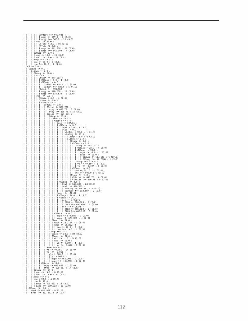
| | | | | | C19dist !<= 569.088 :| | | | | | | mtpy <= 567.2 : 4 (3.0)| | | | | | | mtpy !<= 567.2 : 22 (3.0)| | | | | coo !<= 22.0 :| | | | | | C17nte > 3.0 : 16 (2.0)| | | | | | C17nte !> 3.0 :| | | | | | | mopx <= 641.308 : 22 (7.0)| | | | | | | mopx !<= 641.308 : 7 (3.0)| | | | C20nop !<= 0.0 :| | | | | coo <= 18.0 : 19 (3.0)| | | | | coo !<= 18.0 : 14 (3.0)| | | C19nop !<= 23.0 :| | | | coo <= 20.0 : 1 (3.0)| | | | coo !<= 20.0 : 7 (2.0)| C4N != 0.0 :| | C11nop <= 0.0 :| | | C16nop <= 0.0 :| | | | C24nop <= 24.0 :| | | | | cto <= 1.0 :| | | | | | C5dist <= 673.933 :| | | | | | | C20nop > 0.0 : 4 (3.0)| | | | | | | C20nop !> 0.0 :| | | | | | | | C2dist <= 128.6 : 2 (3.0)| | | | | | | | C2dist !<= 128.6 : 5 (4.0)| | | | | | C5dist !<= 673.933 :| | | | | | | mopy <= 515.538 : 17 (2.0)| | | | | | | mopy !<= 515.538 : 1 (2.0)| | | | | cto !<= 1.0 :| | | | | | C13nte > 0.0 : 4 (2.0)| | | | | | C13nte !> 0.0 :| | | | | | | C14nte <= 3.0 :| | | | | | | | C19nte <= 0.0 :| | | | | | | | | C8dist <= 391.261 :| | | | | | | | | | mtpy <= 495.75 : 5 (2.0)| | | | | | | | | | mtpy !<= 495.75 : 15 (2.0)| | | | | | | | | C8dist !<= 391.261 :| | | | | | | | | | C3nop <= 23.0 :| | | | | | | | | | | C1nop <= 24.0 :| | | | | | | | | | | | C24nte <= 0.0 :| | | | | | | | | | | | | dcoc <= 167.61 :| | | | | | | | | | | | | | C20nte <= 3.0 :| | | | | | | | | | | | | | | C4h3 > 0.0 : 1 (2.0)| | | | | | | | | | | | | | | C4h3 !> 0.0 :| | | | | | | | | | | | | | | | oldCity > 23.0 : 1 (4.0)| | | | | | | | | | | | | | | | oldCity !> 23.0 :| | | | | | | | | | | | | | | | | C18nop > 3.0 : 4 (2.0)| | | | | | | | | | | | | | | | | C18nop !> 3.0 :| | | | | | | | | | | | | | | | | | C11nte <= 3.0 :| | | | | | | | | | | | | | | | | | | C10nop <= 0.0 :| | | | | | | | | | | | | | | | | | | | C14nop <= 113.071 :| | | | | | | | | | | | | | | | | | | | | C16nop > 23.0 : 4 (6.0)| | | | | | | | | | | | | | | | | | | | | C16nop !> 23.0 :| | | | | | | | | | | | | | | | | | | | | | mopx <= 16.0 : 1 (2.0)| | | | | | | | | | | | | | | | | | | | | | mopx !<= 16.0 :| | | | | | | | | | | | | | | | | | | | | | | C13nop <= 14.7648 : 4 (27.0)| | | | | | | | | | | | | | | | | | | | | | | C13nop !<= 14.7648 : 1 (2.0)| | | | | | | | | | | | | | | | | | | | C14nop !<= 113.071 :| | | | | | | | | | | | | | | | | | | | | vy <= -0.197 : 4 (2.0)| | | | | | | | | | | | | | | | | | | | | vy !<= -0.197 : 1 (9.0)| | | | | | | | | | | | | | | | | | | C10nop !<= 0.0 :| | | | | | | | | | | | | | | | | | | | cto <= 501.0 : 1 (2.0)| | | | | | | | | | | | | | | | | | | | cto !<= 501.0 : 4 (2.0)| | | | | | | | | | | | | | | | | | C11nte !<= 3.0 :| | | | | | | | | | | | | | | | | | | C17dist <= 446.75 : 4 (2.0)| | | | | | | | | | | | | | | | | | | C17dist !<= 446.75 : 5 (2.0)| | | | | | | | | | | | | | C20nte !<= 3.0 :| | | | | | | | | | | | | | | C4h3 <= 540.333 : 23 (2.0)| | | | | | | | | | | | | | | C4h3 !<= 540.333 :| | | | | | | | | | | | | | | | oldCity <= 938.667 : 4 (4.0)| | | | | | | | | | | | | | | | oldCity !<= 938.667 : 2 (2.0)| | | | | | | | | | | | | dcoc !<= 167.61 :| | | | | | | | | | | | | | C5nop > 24.0 : 4 (2.0)| | | | | | | | | | | | | | C5nop !> 24.0 :| | | | | | | | | | | | | | | dco <= 6.08276 :| | | | | | | | | | | | | | | | C4h3 <= 490.609 : 2 (2.0)| | | | | | | | | | | | | | | | C4h3 !<= 490.609 : 1 (2.0)| | | | | | | | | | | | | | | dco !<= 6.08276 :| | | | | | | | | | | | | | | | C4h3 <= 485.923 : 1 (14.0)| | | | | | | | | | | | | | | | C4h3 !<= 485.923 : 5 (9.0)| | | | | | | | | | | | C24nte !<= 0.0 :| | | | | | | | | | | | | mopx <= 579.885 : 2 (2.0)| | | | | | | | | | | | | mopx !<= 579.885 : 4 (2.0)| | | | | | | | | | | C1nop !<= 24.0 :| | | | | | | | | | | | dcuc > 14.2127 : 1 (6.0)| | | | | | | | | | | | dcuc !> 14.2127 :| | | | | | | | | | | | | coo <= 19.0 : 4 (3.0)| | | | | | | | | | | | | coo !<= 19.0 : 1 (2.0)| | | | | | | | | | C3nop !<= 23.0 :| | | | | | | | | | | C3nop <= 24.0 : 23 (2.0)| | | | | | | | | | | C3nop !<= 24.0 :| | | | | | | | | | | | dco <= 11.0 : 5 (2.0)| | | | | | | | | | | | dco !<= 11.0 :| | | | | | | | | | | | | vx <= 0.087 : 1 (4.0)| | | | | | | | | | | | | vx !<= 0.087 : 2 (2.0)| | | | | | | | C19nte !<= 0.0 :| | | | | | | | | vx <= -0.051 : 24 (3.0)| | | | | | | | | vx !<= -0.051 :| | | | | | | | | | ply > 568.0 : 1 (3.0)| | | | | | | | | | ply !> 568.0 :| | | | | | | | | | | mopy <= 465.208 : 2 (2.0)| | | | | | | | | | | mopy !<= 465.208 : 5 (2.0)| | | | | | | C14nte !<= 3.0 :| | | | | | | | mtpy <= 409.667 : 1 (2.0)| | | | | | | | mtpy !<= 409.667 : 17 (2.0)| | | | C24nop !<= 24.0 :| | | | | coo <= 19.0 : 5 (3.0)| | | | | coo !<= 19.0 : 22 (2.0)| | | C16nop !<= 0.0 :| | | | coo > 22.0 : 4 (2.0)| | | | coo !> 22.0 :| | | | | mopx <= 609.833 : 14 (2.0)| | | | | mopx !<= 609.833 : 15 (2.0)| | C11nop !<= 0.0 :| | | mopx <= 611.571 : 9 (2.0)| | | mopx !<= 611.571 : 17 (2.0)
112

Bibliography
[Ada94] Andrew Adamatzky. Identification of Cellular Automata. Taylor and Francis Ltd,
1994.
[Amd67] G. M. Amdahl. Validity of the single-processor approach to achieving large scale
computing capabilities. In AFIPS Conference Proceedings, volume 30, pages 483–
485, Reston, Va., 1967. AFIPS Press.
[AW04] Justin Ammerlaan and David Wright. Adaptive cooperative fuzzy logic controller.
In Proceedings of the 27th conference on Australasian computer science, volume 26,
pages 255–263, 2004.
[Bax94] Gregory A. Baxes. Digital Image Processing. John Wiley & Sons, 1994.
[BBI01] Dimitri Burago, Yuri Burago, and Sergei Ivanov. A Course in Metric Geometry.
American Mathematical Society, 2001.
[BL01] Nathaniel E. Baughman and Brian Neil Levine. Cheat-proof playout for centralized
and distributed online games. In INFOCOM, pages 104–113, 2001.
[Bro03] Mark Brockington. Building a reputation system: Hatred, forgiveness, and sur-
render in Neverwinter Nights. In Thor Alexander, editor, Massively Multiplayer
Game Development, pages 454–563. Charles River Media, 2003.
[CDNR04] Andy Collins, Jesse Decker, David Noonan, and Rich Redman. Unearthed Arcana.
Wizards of the Coast, 2004.
[CFK01] E. Cronin, B. Filstrup, and A. Kurc. A distributed multiplayer game server system,
2001.
113

Bibliography
[CFKJ02] Eric Cronin, Burton Filstrup, Anthony R. Kruc, and Sugih Jamin. An efficient
synchronization mechanism for mirrored game architectures. In Proceedings of the
1st workshop on Network and system support for games, pages 67–73. ACM Press,
2002.
[CM98] David Carmel and Shaul Markovitch. Model-based learning of interaction strate-
gies in multiagent systems. Journal of Experimental and Theoretical Artificial
Intelligence, 10(3):309–332, 1998.
[Com03] IGDA Online Games Committee. Online games whitepaper. In Proceedings of
Game Developers Conference, 2003.
[Com04] IGDA Online Games SIG Steering Committee. 2004 persistent worlds whitepaper,
2004.
URL: <http://www.igda.org/online>.
[Dag92] L. Dagum. Three-dimensional direct particle simulation on the connection machine.
Journal of Thermophysics and Heat Transfer, 6(4):637, 1992.
[DdOC03] P Demasi and A. J. de O. Cruz. Online coevolution for action games. IJIGS:
International Journal of Intelligent Games & Simulation, 2(2):80–88, 2003.
[Del] Chrysanthos Dellarocas. The design of reliable trust management systems for
electronic trading communities.
URL: <citeseer.ist.psu.edu/380109.html>.
[Del01] C. Dellarocas. Analyzing the economic efficiency of eBay-like online reputation
reporting mechanisms. In Proceedings of the ACM Conference on Electronic Com-
merce, Tampa, Florida, 2001.
[Den04] Alexandre Denault. Minueto, 2004.
URL: <http://minueto.cs.mcgill.ca/>.
[DG99] C. Diot and L. Gautier. A distributed architecture for multiplayer interactive
applications on the Internet, 1999.
URL: <citeseer.ist.psu.edu/diot99distributed.html>.
[DGGZ03] D. Dutta, A. Goel, R. Govindan, and H. Zhang. The design of a distributed rating
scheme for peer-to-peer systems, 2003.
URL: <citeseer.ist.psu.edu/dutta03design.html>.
114

Bibliography
[DHS00] Richard O. Duda, Peter E. Hart, and David G. Stork. Pattern Classification.
Wiley-Interscience, 2nd edition, 2000.
[DZG93] M.J.P. Devasconcelos, B.P. Zeigler, and L.A. Graham. Modeling multiscale spatial
ecological processes under the discrete-event systems paradigm. Landscape Ecology,
8(4):273–286, 1993.
[EMP+98] David S. Ebert, F. Kenton Musgrave, Darwyn Peachey, Ken Perlin, and Steven
Worley. Texturing and Modeling: A Procedural Approach. Morgan Kaufmann
Publishers, 2nd Bk&Cdr edition, September 1998.
[Ent04] NASA Earth Science Enterprise. GSFC earth science enterprise water and energy
cycle. http://gwec.gsfc.nasa.gov, 2004.
[Fun96] T. Funkhouser. Network topologies for scalable multi-user virtual environments.
Proceedings of VRAIS’96, Santa Clara CA, pages 222–229, 1996.
[FvDFH95] James D. Foley, Andries van Dam, Steven K. Feiner, and John F. Hughes. Com-
puter Graphics: Principles and Practice in C. Addison-Wesley, 2nd edition, 1995.
[Gar70] Martin Gardner. The fantastic combinations of John Conway’s new solitaire game
’Life’. Scientific American, October 1970.
[Guh] R. Guha. Open rating systems.
URL: <citeseer.ist.psu.edu/694373.html>.
[GWJT97] Jianjian Gong, Grace Wahba, Donald R. Johnson, and Joseph Tribbia. Adap-
tive tuning of numerical weather prediction models: Simultaneous estimation of
weighting, smoothing and physical parameters. Technical Report 963r, Univeristy
of Wisconsin, 1997.
URL: <citeseer.ist.psu.edu/99164.html>.
[HAKB96] M. Hadjimichael, P. Arunas, L. Kuciauskas, and R. Brody. Medex: A fuzzy system
for forecasting mediterranean gale force winds, 1996.
URL: <citeseer.ist.psu.edu/hadjimichael96medex.html>.
[HD03] Gordon Hayward and Valerie Davidson. Fuzzy logic applications. Analyst,
128:1304–1306, 2003.
115

Bibliography
[HM89] D. P. Helmbold and C. E. McDowell. Modeling speedup(n) greater than n. In
1989 International Conference on Parallel Processing Proceedings, volume 3, pages
219–225, 1989.
[HM95] Bill Hirsti and Benoit Mandelbrot. Fractal Landscapes from the Real World. Cor-
nerhouse, December 1995.
[HTF01] Trevor Hastie, Robert Tibshirani, and Jerome Friedman. The elements of statistical
learning. Springer, 2001.
[HW95] Thomas D. Haynes and Roger L. Wainwright. A simulation of adaptive agents
in hostile environment. In K. M. George, Janice H. Carroll, Ed Deaton, Dave
Oppenheim, and Jim Hightower, editors, Proceedings of the 1995 ACM Symposium
on Applied Computing, pages 318–323, Nashville, USA, 1995. ACM Press.
[Jak] Mikael Jakobsson. The Sopranos meets Everquest: Social networking in massively
multiplayer online games.
URL: <http://hypertext.rmit.edu.au/dac/papers/Jakobsson.pdf>.
[KMN88] Alex D. Kelley, Michael C. Malin, and Gregory M. Nielson. Terrain simulation
using a model of stream erosion. In Proceedings of the 15th annual conference on
Computer graphics and interactive techniques, pages 163–268, 1988.
[KSGM03] Sepandar D. Kamvar, Mario T. Schlosser, and Hector Garcia-Molina. The Eigen-
Trust algorithm for reputation management in P2P networks. In Proceedings of
the Twelfth International World Wide Web Conference, 2003., 2003.
[Lan03] Marc Lanctot. hexIT: A Java API for using and drawing hexagonal grids, 2003.
URL: <http://www.sable.mcgill.ca/~mlanct2/projects/hexIT-0.61.tar.gz>.
[Lew87] J.P. Lewis. General stochastic subdivision. ACM Transactions on Graphics, July
1987.
[LG01] Barbara Liskov and John Guttag. Program Development in Java: Abstraction,
Specification, and Object-Oriented Design. Addison-Wesley, 2001.
[Mam74] E.H. Mamdani. Applications of fuzzy algorithms for simple dynamic plant. In
Proceedings of IEE, volume 121, pages 1585–1588, 1974.
[Mar94] S. Marsh. Formalising trust as a computational concept, 1994.
URL: <citeseer.ist.psu.edu/marsh94formalising.html>.
116

Bibliography
[Mar99] Kai Martin. Using bitmaps for automatic generation of large-scale terrain models.
Game Developer Magazine, October 1999.
[Mau00] Martin Mauve. How to keep a dead man from shooting. In Interactive Distributed
Multimedia Systems and Telecommunication Services, pages 199–204, 2000.
[McC00] Mason McCuskey. Fuzzy logic for video games. In Mark DeLoura, editor, Game
Programming Gems, pages 319–329. Charles River Media, 2000.
[Mel03] Lary Mellon. Research opportunities in game development. Tutorial at: PADS’03
Workshop on Parallel and Distributed Simulation, June 2003.
[mer] [email protected].
URL: <http://eq.stratics.com/content/statistics/faction/>.
[MFW02] Martin Mauve, Stefan Fischer, and Jorg Widmer. A generic proxy system for
networked computer games. In NETGAMES ’02: Proceedings of the 1st workshop
on Network and system support for games, pages 25–28. ACM Press, 2002.
[Mil85] D.L. Mills. Request for comments (rfc) 958, September 1985.
URL: <http://www.faqs.org/rfcs/rfc958.html>.
[Mit97] Tom Mitchell. Machine Learning. McGraw Hill, 1997.
[NC01] M. Namee and B. Cunningham. A proposal for an agent architecture for proactive
persistent non player characters, 2001.
URL: <citeseer.ist.psu.edu/macnamee01proposal.html>.
[O’N01] Sean O’Neil. A real-time procedural universe, March 2001.
URL: <www.gamasutra.com>.
[Pan] Luca Pancallo. Planeshift.
URL: <http://www.planeshift.it>.
[PdLV02] Ernesto Posse, Juan de Lara, and Hans Vangheluwe. Processing causal block di-
agrams with graph-grammars in AToM3. European Joint Conference on Theory
and Practice of Software (ETAPS), Workshop on Applied Graph Transformation
(AGT), pages 23–34, 2002.
[Pon04] Marc Ponsen. Improving adaptive game AI with evolutionary learning, July 2004.
URL: <http://www.kbs.twi.tudelft.nl/Publications/MSc/2004-Ponsen-MSc.html>.
117

Bibliography
[Qua03] Quazal. Quazal Eterna 2.1 technical overview, November 2003.
URL: <http://www.quazal.com/>.
[Qui92] J. R. Quinlan. C4.5 release 8, 1992.
URL: <http://www2.cs.uregina.ca/~hamilton/courses/831/notes/ml/
dtrees/c4.5/tutorial.html>.
[Rey94] Craig W. Reynolds. Competition, coevolution and the game of tag, 1994.
[RGT00] Bohdana Ratitch, Ricard Gavalda, and Denis Therien. Approximation of real-
valued functions with fuzzy cellular automata. Technical report, McGill University,
2000.
[RHG03] Edwin Rojas, Robert J. Hijmans, and Luigi Guarino. DIVA-GIS, 2003.
URL: <http://diva.riu.cip.cgiar.org/index.php>.
[RN02] Stuart Russell and Peter Norvig. Artificial Intelligence. Prentice-Hall, 2nd edition,
2002.
[RRER03] V. Ramakrishna, Max Robinson, Kevin Eustice, and Peter Reiher. An active
self-optimizing multiplayer gaming architecture. Autonomic Computing Workshop
Fifth Annual International Workshop on Active Middleware Services (AMS’03),
June 2003.
[Ruc02] Rudy Rucker. Software Engineering and Computer Games. Addison-Wesley,
November 2002.
[SB98] Richard S. Sutton and Andrew G. Barto. Reinforcement Learning: An Introduction.
MIT Press, March 1998.
[SKH02] Jouni Smed, Timo Kaukoranta, and Harri Hakonen. A review on networking and
multiplayer computer games. Technical Report 454, Turku Centre for Computer
Science, April 2002.
[SSKP03] Peter Spronk, Ida Sprinkkhuizen-Kuyper, and Eric Postma. Online adaptation of
game opponent AI in simulation and in practice. Game-On, 2003.
[Sta96] Mizuko Ito Stanford. Uses and subversions of SimCity 2000, October 1996.
URL: <http://citeseer.ist.psu.edu/524388.html>.
[Ste94] L. Steels. The artificial life roots of artificial intelligence, 1994.
118

Bibliography
[Str01] Steven H. Strogatz. Nonlinear Dynamics and Chaos: With Applications to Physics,
Biology, Chemistry and Engineering. Perseus Books Group, 2001.
[SZ99] Sandeep Singhal and Michael Zyda. Networked Virtual Environments: Design and
Implementation. Addison-Wesley Professional, September 1999.
[TiH00] Tsuyoshi Taki and Jun ichi Hasegawa. Visualization of dominant region in team
games and its application to teamwork analysis. In Computer Graphics Interna-
tional, pages 227–, 2000.
[Tou] Godfried Toussaint. Grids, connectivity, and contour-tracing.
URL: <http://www-cgrl.cs.mcgill.ca/~godfried/teaching/pr-notes/contour.ps>.
[Tou80] G. Toussaint. The relative neighbourhood graph of a finite planar set, 1980.
[Tou91] G. Toussaint. Some unsolved problems on proximity graphs, 1991.
URL: <citeseer.ist.psu.edu/toussaint91some.html>.
[Toz02] P. Tozour. The perils of AI scripting. In S. Rabin, editor, AI Game Programming
Wisdom, pages 541–547. Charles River Media, 2002.
[vNB66] John von Neumann and A. W. Birks. Theory of Self-Reproducing Automata. Uni-
versity of Illinois Press, Urbana, Illinois, 1966.
[VV00] Hans Vangheluwe and Ghislain C. Vansteenkiste. The cellular automata formalism
and its relationship to DEVS. 14th European Simulation Multi-conference (ESM),
pages 800–810, May 2000.
[Wan96] Li-Xin Wang. A course in Fuzzy Systems and Control. Prentice Hall PTR, 1st
edition, 1996.
[WC03] Gabriel A. Wainer and Wenhong Chena. A framework for remote execution and
visualization of cell-DEVS models. Simulation, 79(11):626–647, 2003.
[WG01] G. Wainer and N. Giambiasi. Timed cell-DEVS: modelling and simulation of cell
spaces, 2001.
URL: <citeseer.ist.psu.edu/wainer01timed.html>.
[WIS96] Dennis D. Wackerly, William Mendenhall III, and Richard L. Scheaffer. Mathe-
matical Statistics with Applications. Wadsworth Publishing Company, 1996.
119

Bibliography
[Wol83] Stephen Wolfram. Cellular automata. Los Alamos Science, 9:2–29, 1983.
[Wol86a] S (Ed.) Wolfram. Theory and Applications of Cellular Automata. World Scientific,
Singapore, 1986.
[Wol86b] Stephen Wolfram. Cellular automata fluids. Journal of Statistical Physics, 45:471–
526, November 1986.
[WP85] Stephen Wolfram and Norman H. Packard. Two-dimensional cellular automata.
Journal of Statistical Physics, 38:901–946, March 1985.
[WZ93] Y. Wang and B. P. Zeigler. DEVS based simulation on a SIMD massively parallel
architecture. Discrete Event Systems, 1993.
[YC02] Jeff Yan and Hyun-Jin Choi. Security issues in online games. The Electronic
Library, 20(2), 2002.
[YS00] Bin Yu and Munindar P. Singh. A social mechanism of reputation management in
electronic communities. In Cooperative Information Agents, pages 154–165, 2000.
[Zad65] L.A. Zadeh. Fuzzy sets. Information and Control, 8:338–353, 1965.
[Zei84] Bernard P. Zeigler. Multifacetted modelling and discrete event simulation. Aca-
demic Press Professional, Inc., 1984.
[ZL04] Cai-Nicolas Ziegler and Georg Lausen. Spreading activation models for trust prop-
agation. In Proceedings of the IEEE International Conference on e-Technology,
e-Commerce, and e-Service, Taipei, Taiwan, March 2004. IEEE Computer Society
Press.
120
Recommended


