arX

iv:s

olv-

int/9

8030

05v1

6 M

ar 1

998

Algorithmic Integrability Tests for Nonlinear

Differential and Lattice Equations 1

Willy Hereman 2,3, Unal Goktas 2,4, Michael D. Colagrosso 2

Department of Mathematical and Computer Sciences, Colorado School of Mines,

Golden, CO 80401-1887, U.S.A.

and Antonio J. Miller 5

Advanced Sensors and Control Department, The Applied Research Laboratory,

The Pennsylvania State University, State College, PA 16804-0030, U.S.A.

Abstract

Three symbolic algorithms for testing the integrability of polynomial systems ofpartial differential and differential-difference equations are presented. The first al-gorithm is the well-known Painleve test, which is applicable to polynomial systemsof ordinary and partial differential equations. The second and third algorithms allowone to explicitly compute polynomial conserved densities and higher-order symme-tries of nonlinear evolution and lattice equations.

The first algorithm is implemented in the symbolic syntax of both Macsyma andMathematica. The second and third algorithms are available in Mathematica. Thecodes can be used for computer-aided integrability testing of nonlinear differentialand lattice equations as they occur in various branches of the sciences and engineer-ing. Applied to systems with parameters, the codes can determine the conditionson the parameters so that the systems pass the Painleve test, or admit a sequenceof conserved densities or higher-order symmetries.

Key words: Integrability; Painleve test; Conservation law; Invariant; Symmetry;Differential equation; Lattice

1 Research supported in part by NSF under Grant CCR-9625421.2 E-mail: {whereman,ugoktas,mcolagro}@mines.edu3 Corresponding author. Phone: (303) 273 3881; Fax: (303) 273 3875.4 Supported in part by Wolfram Research, Inc.5 E-mail: ajmiller@sabine.acs.psu.edu

Preprint submitted to Elsevier Preprint 9 February 2008

1 Introduction

During the last three decades, the study of integrability, invariants, symme-tries, and exact solutions of nonlinear ordinary and partial differential equa-tions (ODEs, PDEs) and differential-difference equations (DDEs) has beenthe topic of major research projects in the dynamical systems and the solitoncommunities.

Various techniques have been developed to determine whether or not PDEsbelong to the privileged class of completely integrable equations [15]. Oneof the most successful and widely applied techniques is the Painleve test,named after the French mathematician Paul Painleve (1863-1933) [35], whoclassified second-order differential equations that are globally integrable interms of elementary functions by quadratures or by linearization. In essence,the Painleve test verifies whether or not solutions of differential equations inthe complex plane are single-valued in the neighborhood of all their movablesingularities.

To a large extent, the Painleve test is algorithmic, yet very cumbersome whendone by hand. In particular, the verification of the compatibility conditions isassessed by many practitioners of the Painleve test as a painstaking compu-tation. In addition to the tedious verification of self-consistency (or compati-bility) conditions, computer programs are helpful at exploring all possibilitiesof balancing singular terms. Indeed, the omission of one or more choices of“dominant behavior” can lead to wrong conclusions [12,44].

We therefore developed the programs painsing.max and painsys.max [25] (bothin Macsyma syntax [36]), and painsing.m and painsys.m in Mathematica lan-guage [53], that perform the Painleve test for polynomial systems of ODEsand PDEs. In this paper we demonstrate the above codes by analyzing afew prototypical nonlinear equations and systems, such as the Boussinesq andnonlinear Schrodinger equations, a class of fifth-order KdV equations, and theHirota-Satsuma and Lorenz systems.

Our computer code does not deal with the theoretical shortcomings of thePainleve test as identified by Kruskal and others [30–32]. Thus far, we haveimplemented the traditional Painleve test [26,27], and not yet incorporatedthe latest advances in Painleve type methods, such as the poly-Painleve test[31] or other generalizations [30,32]. Neither did we code the weak Painlevetest [43,44] or other variants [9–11,17]. Furthermore, we do not have code forthe singularity confinement method [23], i.e. an adaptation of the Painlevetest that allows one to test the integrability of difference equations.

Among the various alternatives to establish the integrability [15] of nonlinearPDEs and DDEs, the search for conserved densities and higher-order symme-

2

tries is particularly appealing. Indeed, in this paper we will give algorithmsthat apply to both the continuous and semi-discrete cases. We implementedthese algorithms [18–20] in Mathematica, but they are fairly simple to code inother computer algebra languages (see [18,20]).

Our algorithms are based on the concept of dilation (scaling) invariance. Thatinherently limits their scope to polynomial conserved densities and higher-order symmetries of polynomial systems. Although the existence of a sequenceof conserved densities predicts integrability, the nonexistence of polynomialconserved quantities does not preclude integrability. Indeed, integrable PDEsor DDEs could be disguised with a coordinate transformation in DDEs thatno longer admit conserved densities of polynomial type [46]. The same careshould be taken in drawing conclusions about non-integrability based on thelack of higher-order symmetries, or equations failing the Painleve test.

Apart from integrability testing, the knowledge of the explicit form of con-served densities and higher-order symmetries is useful. For instance, withhigher-order symmetries of integrable systems, one can build new completelyintegrable systems, or discover connections between integrable equations andtheir group theoretic origin.

Explicit forms of conserved densities are useful in the numerical solution ofPDEs or DDEs. In solving DDEs, which may arise from integrable discretiza-tions of PDEs, one should check that conserved quantities indeed remain con-stant. In particular, the conservation of a positive definite quadratic quantitymay prevent nonlinear instabilities in the numerical scheme.

Our integrability package InvariantsSymmetries.m [21] in Mathematica au-tomates the tedious computation of closed-form expressions for conserveddensities and higher-order symmetries for both PDEs and DDEs. Appliedto systems with parameters, the package determines the conditions on theseparameters so that a sequence of conserved densities or symmetries exists.The software can thus be used to test the integrability of classes of equationsthat model various wave phenomena. Our examples include a vector modifiedKdV equation, the extended Lotka-Volterra and relativitic Toda lattices, andthe Heisenberg spin model.

The conserved densities and symmetries presented in this paper were obtainedwith InvariantsSymmetries.m.

3

2 Symbolic Program for the Painleve Test

2.1 Purpose

We focus on PDEs. As originally formulated by Ablowitz et al. [2,3], thePainleve conjecture asserts that all similarity reductions of a completely in-tegrable PDE should be of Painleve-type; i.e. its solutions should have nomovable singularities other than “poles” in the complex plane.

A later version of the Painleve test due to Weiss et al. [52] allows testing of thePDE directly, without recourse to the reduction(s) to an ODE. A PDE is saidto have the Painleve property [1] if its solutions in the complex plane are single-valued in the neighborhood of all its movable singularities. In other words, theequation must have a solution without any branching around the singularpoints whose positions depend on the initial conditions. For ODEs, it sufficesto show that the general solution has no worse singularities than movablepoles, or that no branching occurs around movable essential singularities.

A three step-algorithm, known as the Painleve test, allows one to verifywhether or not a given nonlinear system of ODEs or PDEs with (real) polyno-mial terms fulfills the necessary conditions for having the Painleve property.Such equations are prime candidates for being completely integrable.

There is a vast amount of literature about the test and its applications to spe-cific ODEs and PDEs. Several well-documented surveys [5,9,15,31,32,34,38,40]and books [8,10,48] discuss subtleties and pathological cases of the test thatare far beyond the scope of this article. Other survey papers [15,16,39] dealwith the many interesting by-products of the Painleve test. For example, theyshow how a truncated Laurent series expansion of the type introduced below,allows one to construct Lax pairs, Backlund and Darboux transformations,and closed-form particular solutions of PDEs.

2.2 Algorithm for a Single Equation

We briefly outline the three steps of the Painleve test for a single PDE,

F(x, t, u(x, t)) = 0, (1)

4

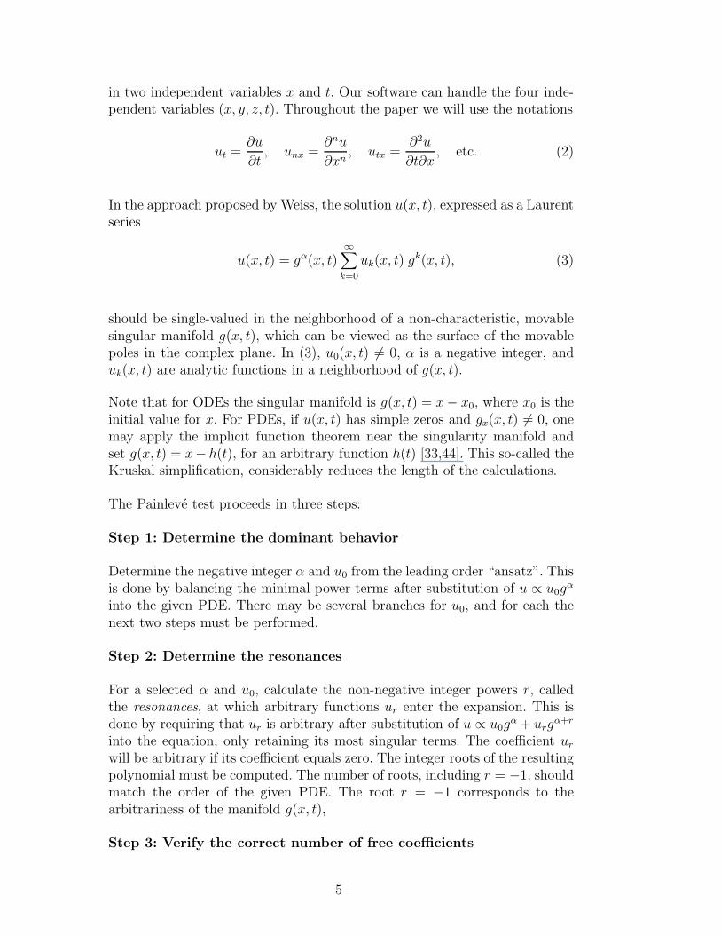
in two independent variables x and t. Our software can handle the four inde-pendent variables (x, y, z, t). Throughout the paper we will use the notations

ut =∂u

∂t, unx =

∂nu

∂xn, utx =

∂2u

∂t∂x, etc. (2)

In the approach proposed by Weiss, the solution u(x, t), expressed as a Laurentseries

u(x, t) = gα(x, t)∞∑

k=0

uk(x, t) gk(x, t), (3)

should be single-valued in the neighborhood of a non-characteristic, movablesingular manifold g(x, t), which can be viewed as the surface of the movablepoles in the complex plane. In (3), u0(x, t) 6= 0, α is a negative integer, anduk(x, t) are analytic functions in a neighborhood of g(x, t).

Note that for ODEs the singular manifold is g(x, t) = x − x0, where x0 is theinitial value for x. For PDEs, if u(x, t) has simple zeros and gx(x, t) 6= 0, onemay apply the implicit function theorem near the singularity manifold andset g(x, t) = x− h(t), for an arbitrary function h(t) [33,44]. This so-called theKruskal simplification, considerably reduces the length of the calculations.

The Painleve test proceeds in three steps:

Step 1: Determine the dominant behavior

Determine the negative integer α and u0 from the leading order “ansatz”. Thisis done by balancing the minimal power terms after substitution of u ∝ u0g

α

into the given PDE. There may be several branches for u0, and for each thenext two steps must be performed.

Step 2: Determine the resonances

For a selected α and u0, calculate the non-negative integer powers r, calledthe resonances, at which arbitrary functions ur enter the expansion. This isdone by requiring that ur is arbitrary after substitution of u ∝ u0g

α + urgα+r

into the equation, only retaining its most singular terms. The coefficient ur

will be arbitrary if its coefficient equals zero. The integer roots of the resultingpolynomial must be computed. The number of roots, including r = −1, shouldmatch the order of the given PDE. The root r = −1 corresponds to thearbitrariness of the manifold g(x, t),

Step 3: Verify the correct number of free coefficients

5

Verify that the correct number of arbitrary functions ur indeed exists by sub-stituting the truncated expansion

u(x, t) = gαrmax∑

k=0

uk(x, t)gk(x, t) (4)

into the PDE, where rmax is the largest resonance. At non-resonance levels,determine all uk. At resonance levels, ur should be arbitrary, and since we aredealing with a nonlinear equation, a compatibility condition must be verified.

An equation for which the above steps can be carried out consistently andunambiguously, is said to have the Painleve property and is conjectured to becompletely integrable. This entails that the solution has the necessary numberof free coefficients ur, and that the compatibility condition at each of theseresonances is unconditionally satisfied.

The reader should be warned that the above algorithm does not detect es-sential singularities and therefore cannot determine whether or not branchingoccurs about these. So, for an equation to be integrable it is not sufficient thatit passes the Painleve test. Neither it is necessary. Indeed, there are integrableequations, such as the Dym-Kruskal equation, ut = u3u3x, that do not pass thePainleve test, yet, by a complicated change of variables can be transformedinto an integrable equation.

2.3 Algorithm for Systems

The generalization of the algorithm to systems of ODEs and PDEs is obvi-ous. Yet, it is non-trivial to implement. One of the reasons is that the majorsymbolic packages do not handle inequalities well.

With respect to systems, our code is based on the above three step-algorithmbut generalized to systems, as it can be found in [33,44,48]. In these papersthere is an abundance of worked examples that served as test cases.

For example, given a system of first-order ODEs,

dui

dx= Gi(u1, u2, ..., un; x), i = 1, 2, ..., n, (5)

one introduces a Laurent series for every dependent variable ui(x) :

ui = (x − x0)αi

∞∑

k=0

u(i)k (x − x0)

k. (6)

6

The computer program must carefully determine all branches of dominantbehavior corresponding to various choices of αi and/or u

(i)0 . For each branch,

the single-valuedness of the corresponding Laurent expansion must be tested(i.e. the resonances must be computed and the compatibility conditions mustbe verified). All the details can be found in [15,33,44].

Singularity analysis for PDEs is nontrivial [32] and the Painleve test shouldbe applied with extreme care. Notwithstanding, our software automaticallyperforms the formal steps of the Painleve test for systems of ODEs and PDEs.The examples in section 3.2 illustrate how the code works. Careful analysisof the output and drawing conclusions about integrability should be done byhumans. Some subtleties of the mathematics of the Painleve test of systemsof PDEs were also dealt with in [6,13,28,49].

3 Examples of the Painleve Test

3.1 Single Equations

Numerous examples of the Painleve test for ODEs can be found in the re-view papers. We turn our attention to PDEs. Using our software packagepainsing.max or painsing.m one can determine the conditions under which theequation

utx + a(t)ux + 6uu2x + 6u2x + u4x = 0, (7)

passes the Painleve test.

For (7), α = −2 and u0 = −2g2x. Apart from r = −1, the roots are r = 4, 5,

and 6. The latter three are resonances. Furthermore,

u1 =2g2x, u2 = − 1

6g2x

(4gxg3x − 3g22x + gtgx), (8)

u3 =1

6g4x

(a(t)g3x + g2

xg4x − 4gxg2xg3x + 3g22x − gtgxg2x + gtxg

2x), (9)

and u4 and u5 are indeed arbitrary since the compatibility conditions at res-onances r = 4 and r = 5 are satisfied identically.

The compatibility condition at resonance r = 6 is at + 2a2 = 0. Ignoring thetrivial solution, we get a = 1

2(t−t0). Without loss of generality, we set t0 = 0 and

equation (7) becomes the cylindrical KdV equation which is indeed completely

7

integrable [1,4]. Painleve based investigations for integrable PDEs with spaceand time dependent coefficients are given in [1,7,24,27].

Our Painleve programs cannot automatically test a class of equations such as

ut + au2ux + buxu2x + cuu3x + u5x = 0, (10)

with arbitrary (non-zero and real) parameters a, b and c. The parameters affectthe lowest coefficient in the Laurent expansion in such as way that the roots(r) cannot be computed, and the integrability conditions can no longer betested.

In (10) there are four cases that are of particular interest:

(i) a = 310

c2 and b = 2c (Lax equation),

(ii) a = 15c2 and b = c (Sawada-Kotera equation),

(iii) a = 15c2 and b = 5

2c (Kaup-Kupershmidt equation), and

(iv) a = 29c2 and b = 2c (Ito equation).

In Table 1 we list the results of the Painleve test applied to these cases. Forthe first three equations the compatibility conditions are satisfied at all theresonances. These equations pass the test. For the Ito equation the compati-bility conditions are only satisfied at some of the resonances. The Ito equationfails the test. The first three equations are known to be completely integrable.Ito’s equation is not completely integrable.

The two other algorithms presented in this paper can determine the conditions(i), (ii) and (iii) that assure the complete integrability of (10). The conserveddensities and higher-order symmetries of (10) can be found in [18] and [20].

8

Lax Sawada-Kotera Kaup−Kupershmidt Ito

(a, b, c)=(30, 20, 10) (a, b, c)=(5, 5, 5) (a, b, c)=(20, 25, 10) (a, b, c)=(2, 6, 3)

α = −2 α = −2 α = −2 α = −2

Branch 1 Branch 1 Branch 1 Branch 1

u0 = −2g2x u0 = −6g2

x u0 = −32g2

x u0 = −6g2x

r=−1, 2, 5, 6, 8 r=−1, 2, 3, 6, 10 r=−1, 3, 5, 6, 7 r=−1, 3, 4, 6, 8

OK for r ≥ 2 OK for r ≥ 2 OK for r ≥ 3 OK at r=3

Not at r=4, 6, 8

Branch 2 Branch 2 Branch 2 Branch 2

u0 = −6g2x u0 = −12g2

x u0 = −12g2x u0 = −30g2

x

r=−3,−1, 6, 8, 10 r=−2,−1, 5, 6,12 r=−7,−1, 6, 10, 12 r=−5,−1, 6, 8,12

OK for r ≥ 6 OK for r ≥ 5 OK for r ≥ 6 OK at r=6, 8

Not at r=12

Passes Test Passes Test Passes Test Fails Test

Table 1: Painleve analysis of fifth-order KdV equationut + au2ux + buxu2x + cuu3x + u5x = 0

3.2 Simple Systems

We start with a famous system of ODEs,

u′

1 = a(u2 − u1), u′

2 = −u1u3 + bu1 − u2, u′

3 = u1u2 − cu3, (11)

where a, b, and c are positive constants. System (11) was proposed by themeteorologist E. N. Lorenz as a simplified model for atmospheric turbulencein a vertical air cell beneath a thunderhead [47].

Using our code painsys.max or painsys.m, with the series (6) for i = 1, 2, 3, wedetermine the leading orders α1 = −1, α2 = α3 = −2. The first coefficients inthe series are

u(1)0 = ±2i, u

(2)0 = ∓2i

a, u

(3)0 = −2

a. (12)

9

The roots are r = −1, 2, 4. Furthermore,

u(1)1 = ∓1

3i(2c − 3a + 1), u

(2)1 = ±2i, u

(3)1 =

2

3a(3a − c + 1). (13)

The compatibility conditions at resonances r = 2 and r = 4 are not satisfied.At resonance r = 2 we encounter the condition a(c − 2a)(c + 3a − 1) = 0. So,we consider two cases:

• For c = 2a, the compatibility condition at r = 4 is not satisfied.• For c = 1 − 3a, the compatibility condition at r = 4 is satisfied

provided that a = 13.

We conclude that the Lorenz system (11) passes the Painleve test when a = 13

and c = 0. This special case may not be relevant in the context of meteorologysince in (11) the parameters a, b, c in (11) are supposed to be positive.

To illustrate the generalization of the algorithm to systems of PDEs, considerthe system

uuxt − uxut + vxvt = 0, uvxt − utvx − uxvt = 0, (14)

which plays a role in elementary particle physics [49]. For any of the dependentvariables we introduce a Laurent expansion

u = gα∞∑

k=0

uk gk, v = gβ∞∑

k=0

vk gk. (15)

Analysis of the dominant behavior leads to α = β = −1 and u20 + v2

0 = 0.Let v0 be arbitrary, then u0 = ±iv0. Next, we look for powers of g at whicharbitrary functions ur, vr can enter. Equating the coefficients of gr−4, r > 0,we obtain the system

2r ir(r − 1)

i(r2 − r + 2) −2(r − 1)

ur

vr

= 0. (16)

The determinant of the coefficient matrix vanishes provided r = −1, 0, 1, 2.Note that r = 0 confirms that v0 can be chosen freely. Upon substitution ofthe Laurent series (truncated at level k = 2) and setting the terms in g−2

and g−3 equal to zero, one finds that u1 is completely determined, whereas v1

and u2 (or v2) are arbitrary. The compatibility conditions are satisfied. TheLaurent expansions have the required number of arbitrary functions uk. Thus,the system (14) passes the Painleve test.

10

Hirota and Satsuma [1] proposed a coupled system of KdV equations,

ut − 6auux + 6vvx − au3x = 0, vt + 3uvx + v3x = 0, (17)

where a is a nonzero parameter. System (17) describes interactions of twolong waves with different dispersion relations. It is known to be completelyintegrable for a = 1

2. This is confirmed by the Painleve test. Indeed, with (15)

we obtain α = β = −2 and r = −2,−1, 3, 4, 6 and 8. Furthermore, u0 = −4and v0 = ±2

√2a, determine the coefficients u1, v1, u2, v2 unambiguously. At

resonances 3 and 4 there is one free function and no condition for a. The coef-ficients u5 and v5 are unique determined, but at resonance 6, the compatibilitycondition is only satisfied if a = 1

2. For this value, the compatibility condition

at resonance 8 is also satisfied.

For the integrable version of the Boussinesq system [45]

ut + vx + uux = 0, vt + u3x + (uv)x = 0, (18)

with the Laurent expansions in (15), the leading order is α = −1, β = −2.Careful investigation of the recursion relations linking the uk and vk allows oneto conclude that there are resonances at levels 2, 3 and 4. Finally, the threecompatibility conditions are seen to hold after lengthy computations. System(18) thus passes the test.

Our codes painsys.max are also applicable to complex equations such as thenonlinear Schrodinger (NLS) equation [1],

iqt − q2x + 2|q|2q = 0, (19)

where q(x, t) is a complex function. First, (19) must be rewritten as a system:

ut − v2x + 2v(u2 + v2) = 0, vt + u2x − 2u(u2 + v2) = 0, (20)

where q = u + iv. For simplicity, we use the Kruskal simplification, settingg(x, t) = x − h(t) in (15). Then, the leading order is α = β = −1, and

r = −1, 0, 3 and 4. Furthermore, v0 = ±√

1 − u20, with u0 arbitrary, and

u1 =1

2v0ht, v1 = −1

2u0ht, u2 = − 1

12v0u0(v0h

2t + 2u0,t),

v2 =− 1

12(v0h

2t + 2u0,t), u3 = − 1

8u0(htt + 8v0v3),

u4 =− 1

24v40

(2v30hthtt − v2

0u0,tt − u0u20,t − 24u0v

30v4), (21)

11

where v3 and v4 are arbitrary. Note that at every resonance there is one freefunction in the Laurent expansion. The NLS equation passes the test.

In searching the literature we found numerous examples of systems for whichthe Painleve test was carried out by hand. Some of the most elaborate exam-ples of Painleve analysis involve three-wave interactions [37], the mixmasteruniverse model [12], and chaotic star pulsations [51].

4 Symbolic Programs for Conserved Densities and Symmetries

4.1 The Key Concepts

The key observation behind our algorithms is that conserved densities andhigher-order symmetries of a PDE or DDE system abide by the dilation sym-metry of that system. We illustrate this for prototypical examples of singlePDEs and DDEs.

Dilation Invariance of PDEs. The ubiquitous Korteweg-de Vries (KdV)equation from soliton theory [1],

ut = 6uux + u3x, (22)

is invariant under the dilation (scaling) symmetry

(t, x, u) → (λ−3t, λ−1x, λ2u), (23)

where λ is an arbitrary parameter. Obviously, u corresponds to two derivativesin x, i.e. u ∼ ∂2/∂x2. Similarly, ∂/∂t ∼ ∂3/∂x3. Introducing weights, denotedby w, we have w(u) = 2 and w(∂/∂t) = 3, provided we set w(∂/∂x) = 1. Therank R of a monomial equals the sum of all of its weights. Observe that (22)is uniform in rank since all the terms have rank R = 5.

Conserved Densities of PDEs. For PDEs like (22), the conservation law

Dtρ + DxJ = 0 (24)

connects the conserved density ρ and the associated flux J. As usual, Dt andDx are total derivatives. With few exceptions, polynomial density-flux pairsonly depend on u,ux, etc., and not explicitly on t and x.

The first three (of infinitely many) independent conservation laws for (22) are

12

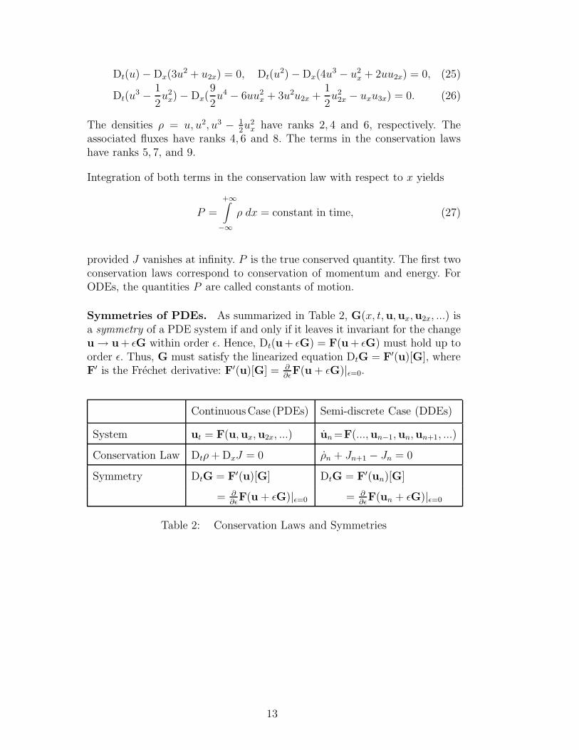
Dt(u) − Dx(3u2 + u2x) = 0, Dt(u

2) − Dx(4u3 − u2

x + 2uu2x) = 0, (25)

Dt(u3 − 1

2u2

x) − Dx(9

2u4 − 6uu2

x + 3u2u2x +1

2u2

2x − uxu3x) = 0. (26)

The densities ρ = u, u2, u3 − 12u2

x have ranks 2, 4 and 6, respectively. Theassociated fluxes have ranks 4, 6 and 8. The terms in the conservation lawshave ranks 5, 7, and 9.

Integration of both terms in the conservation law with respect to x yields

P =

+∞∫

−∞

ρ dx = constant in time, (27)

provided J vanishes at infinity. P is the true conserved quantity. The first twoconservation laws correspond to conservation of momentum and energy. ForODEs, the quantities P are called constants of motion.

Symmetries of PDEs. As summarized in Table 2, G(x, t,u,ux,u2x, ...) isa symmetry of a PDE system if and only if it leaves it invariant for the changeu → u + ǫG within order ǫ. Hence, Dt(u + ǫG) = F(u + ǫG) must hold up toorder ǫ. Thus, G must satisfy the linearized equation DtG = F′(u)[G], whereF′ is the Frechet derivative: F′(u)[G] = ∂

∂ǫF(u + ǫG)|ǫ=0.

ContinuousCase (PDEs) Semi-discrete Case (DDEs)

System ut = F(u,ux,u2x, ...) un =F(...,un−1,un,un+1, ...)

Conservation Law Dtρ + DxJ = 0 ρn + Jn+1 − Jn = 0

Symmetry DtG = F′(u)[G] DtG = F′(un)[G]

= ∂∂ǫ

F(u + ǫG)|ǫ=0 = ∂∂ǫ

F(un + ǫG)|ǫ=0

Table 2: Conservation Laws and Symmetries

13

Two nontrivial higher-order symmetries [42] of (22) are

G(1)=30u2ux + 20uxu2x + 10uu3x + u5x, (28)

G(2)=140u3ux + 70u3x + 280uuxu2x + 70u2u3x + 70u2xu3x + 42uxu4x

+14uu5x + u7x. (29)

The recursion operator [42, p. 312],

Φ = D2 + 4u + 2uxD−1, (30)

connects the above symmetries, Φ G(1) = G(2), and also the lower order sym-metries as shown in [20].

Note that the recursion operator (30) is also uniform in rank with R = 2 sincew(D−1) = −1. Currently, we are working on an algorithm and symbolic codeto compute recursion operators based on the knowledge of a few higher-ordersymmetries and conserved densities.

Higher-order symmetries lead to new integrable PDEs. Indeed, the evolutionequations ut = G(1) and ut = G(2) are the well-known fifth and seventh-orderequations in the completely integrable KdV hierarchy [1].

Dilation Invariance of DDEs. We now turn to the semi-discrete case. Asprototype, consider the Volterra lattice [1],

un = un (un+1 − un−1). (31)

which is one of the discretizations of (22). Note that (31) is invariant under

(t, un) → (λ−1t, λun). (32)

So, un ∼ d/dt, or w(un) = 1 if we set w(d/dt) = 1. Every term in (31) hasrank R = 2, thus (31) is uniform in rank.

Conserved Densities of DDEs. For DDEs like (31), the conservation law

ρn + Jn+1 − Jn = 0 (33)

connects the conserved density ρn and the associated flux Jn. For (31) thefirst two conservation laws (of ranks 2 and 3) are

d

dt(un) + unun−1 − un+1un = 0, (34)

14

d

dt(1

2u2

n + unun+1) + un−1u2n + un−1unun+1 − unu

2n+1 − unun+1un+2 = 0. (35)

The densities ρn = un and ρn = un (12un + un+1) have ranks 1 and 2. Their

fluxes Jn = −unun−1 and Jn = −un−1u2n − un−1unun+1 have ranks 2 and 3.

Symmetries of DDEs. For DDEs of type (31), G(...,un−1,un,un+1, ...) isa symmetry if and only if the infinitesimal transformation un → un + ǫGleaves the DDE invariant within order ǫ. Consequently, G must satisfy dG

dt=

F′(un)[G], where F′ is the Frechet derivative, F′(un)[G] = ∂∂ǫ

F(un + ǫG)|ǫ=0.See Table 2.

The first nontrivial higher-order symmetry of (31) is

G = unun+1 (un + un+1 + un+2) − un−1un (un−2 + un−1 + un), (36)

and, similar to the continuous case, an integrable lattice un = G follows.

Both (22) and (31) have infinitely many polynomial conserved densities [18,22]and symmetries [20].

Remarks:

(i) For scaling invariant systems like (22) and (31), it suffices to consider thedilation symmetry on the space of independent and dependent variables.

(ii) For systems that are inhomogeneous under a suitable scaling symmetrywe use the following trick: We introduce one (or more) auxiliary parameter(s)with appropriate scaling. In other words, we extend the action of the dilationsymmetry to the space of independent and dependent variables, including theparameters. These extra parameters should be viewed as additional dependentvariables, with the caveat that their derivatives are zero. With this trick we canapply our algorithms to a larger class of polynomial PDE and DDE systems.Examples can be found in [18–20,22].

Scaling (dilation) invariance, which is a special Lie-point symmetry, is commonto many integrable nonlinear PDEs and DDEs. In the next two sections weshow how the scaling invariance can be explicitly used to compute polynomialconserved densities and higher-order symmetries of PDEs and DDEs.

4.2 Algorithms for the Computation of Conserved Densities

PDE Case. Conserved densities of PDEs can be computed as follows:

15

• Require that each equation in the system of PDEs is uniform in rank. Solvethe resulting linear system to determine the weights of the dependent variables.For instance for (22), solve w(u) + w(∂/∂t) = 2w(u) + 1 = w(u) + 3, to getw(u) = 2 and w(∂/∂t) = 3.

• Select the rank R of ρ, say, R = 6. Make a linear combination of all themonomials in the components of u and their x-derivatives that have rank R.Remove all monomials that are total x-derivatives (like u4x). Remove equiv-alent monomials, that is, those that only differ by a total x-derivative. Forexample, uu2x and u2

x are equivalent since uu2x = 12(u2)2x − u2

x. For (22), onegets ρ = c1u

3 + c2u2x of rank R = 6.

• Substitute ρ into the conservation law (24). Use the PDE system to eliminateall t-derivatives, and require that the resulting expression E is a total x-derivative. Apply the Euler operator (see [18] for the general form),

Lu =∂

∂u− Dx(

∂

∂ux

) + D2x(

∂

∂u2x

) + · · · + (−1)nDnx(

∂

∂unx

) (37)

to E to avoid integration by parts. If any terms remain, they must vanishidentically. This yields a linear system for the constants ci. Solve the system.For (22), one gets c1 = 1, c2 = −1/2.

See [18] for the complete algorithm and its implementation.

DDE Case. The computation of conserved densities proceeds as follows:

• Compute the weights in the same way as for PDEs. For (31), one getsw(un) = 1 by solving w(un)+1 = 2w(un). Note that w(d/dt) = 1 and weightsare independent of n.

• Determine all monomials of rank R in the components of un and theirt-derivatives. Use the DDE to replace all the t-derivatives. Monomials areequivalent if they belong to the same equivalence class of shifted monomials.For example, un−1vn+1, un+2vn+4 and un−3vn−1 are equivalent. Keep only themain representatives (centered at n) of the various classes.

• Combine these representatives linearly with coefficients ci, and substitutethe form of ρn into the conservation law ρn = Jn − Jn+1.

• Remove all t-derivatives and pattern-match the resulting expression withJn − Jn+1. To do so use the following equivalence criterion: if two monomialsm1 and m2 are equivalent, m1 ≡ m2, then m1 = m2 + [Mn −Mn+1] for somepolynomial Mn that depends on un and its shifts. For example, un−2un ≡un−1un+1 since un−2un = un−1un+1 +[un−2un −un−1un+1] = un−1un+1 +[Mn −

16

Mn+1], with Mn = un−2un. Set the non-matching part equal to zero, and solvethe linear system for the ci. Determine Jn from the pattern Jn − Jn+1. For(31), the first three (of infinitely many) densities ρn are listed in Table 3.

KdV Equation Volterra Lattice

Equation ut = 6uux + u3x un = un (un+1 − un−1)

Densities ρ = u, ρ = u2 ρn = un, ρn = un (12un + un+1)

ρ = u3 − 12u2

x ρn = 13u3

n+ unun+1(un+ un+1+ un+2)

Symmetries G=ux, G=6uux + u3x G = unun+1 (un + un+1 + un+2)

G=30u2ux + 20uxu2x −un−1un(un−2 + un−1 + un)

+10uu3x + u5x

Table 3: Prototypical Examples

Details about this algorithm and its implementation are in [19,22]. See [21] foran integrated Mathematica Package that computes conserved densities (andalso symmetries) of PDEs and DDEs.

4.3 Algorithm for the Computation of Symmetries

PDE Case. Higher-order (or generalized symmetries) of PDEs can be com-puted as follows:

• Determine the weights of the dependent variables in the system.

• Select the rank R of the symmetry. Make a linear combination of all themonomials involving u and its x-derivatives of rank R. For example, for (22),G = c1 u2ux+c2 uxu2x+c3 uu3x+c4 u5x is the form of the generalized symmetryof rank R = 7. In contrast to the computation of conserved densities, no termsare removed here.

• Compute DtG. Use the PDE system to remove all t-derivatives. Equate theresult to the Frechet derivative F′(u)[G]. Treat the different monomial termsin u and its x-derivatives as independent, to get the linear system for ci. Solvethat system. For (22), one obtains

G = 30u2ux + 20uxu2x + 10uu3x + u5x. (38)

The symmetries of the Lax family of rank 3, 5, and 7 are listed in Table 3.They are the first three of infinitely many. See [20] for the details about the

17

algorithm.

18

DDE Case. Higher-order symmetries of DDEs can be computed as follows:

• First determine the weights of the variables in the DDE the same way asfor conserved densities.

• Determine all monomials of rank R in the components of un and theirt-derivatives. Use the DDE to replace all the t-derivatives. Make a linear com-bination of the resulting monomials with coefficients ci.

• Compute DtG and remove all un−1, un, un+1, etc. Equate the resulting ex-pression to the Frechet derivative F′(un)[G] and solve the system for the ci,treating the monomials in un and its shifts as independent.

For (31), the symmetry G of rank R = 3 is listed in Table 3. There areinfinitely many symmetries, all with different ranks.

See [20] for the complete algorithm and its implementation in Mathematica,and [21] for an integrated Mathematica Package that computes symmetries ofPDEs and DDEs.

Notes:

(i) A slight modification of these methods allows one to find conserved densitiesand symmetries of PDEs that explicitly depend on t and x. See the firstexample in the next section.

(ii) Applied to systems with free parameters, the linear system for the ci

will depend on these parameters. A careful analysis of the eliminant leadsto conditions on these parameters so that a sequence of conserved densitiesor symmetries exists. Details about this type of analysis and its computerimplementation can be found in [18].

5 Examples of Densities and Symmetries

5.1 Vector Modified KdV Equation

In [50], Verheest investigated the integrability of a vector form of the modifiedKdV equation (vmKdV),

Bt + (|B|2B)x + Bxxx = 0, (39)

or component-wise for B = (u, v),

19

ut + 3u2ux + v2ux + 2uvvx + u3x = 0,

vt + 3v2vx + u2vx + 2uvux + v3x = 0. (40)

With our software InvariantsSymmetries.m [21] we computed

ρ1 = u, ρ2 = v, ρ3 = u2 + v2, ρ4 =1

2(u2 + v2)2 − (u2

x + v2x), (41)

ρ5 =1

3x(u2 + v2) − 1

2t(u2 + v2)2 + t(u2

x + v2x). (42)

Note that the latter density depends explicitly on x and t. Verheest [50] hasshown that (40) is non-integrable for it lacks a bi-Hamiltonian structure andrecursion operator. We were unable to find additional polynomial conserveddensities. Polynomial higher-order symmetries for (40) do not appear to exist.

5.2 Heisenberg Spin Model

The continuous Heisenberg spin system [14] or Landau-Lifshitz equation,

St = S× ∆S + S× DS, (43)

models a continuous anisotropic Heisenberg ferromagnet. It is considered auniversal integrable system since various known integrable PDEs, such as theNLS and sine-Gordon equations, can be derived from it. In (43), S = [u, v, w]T

with real components, ∆ = ∇2 is the Laplacian, D is a diagonal matrix, and× is the standard cross product of vectors.

Split into components, (43) reads

ut = vw2x − wv2x + (β − α)vw,

vt = wu2x − uw2x + (1 − β)uw,

wt = uv2x − vu2x + (α − 1)uv. (44)

In Table 4 we list the conserved densities for three typical cases; other casesare similar.

Note that for all the cases we considered

ρ = u2 + v2 + w2 = ||S||2 (45)

is constant in time (since J = 0). Hence, all even powers of ||S|| are alsoconserved densities, but they are dependent of (45).

20

D = diag(1, α, β) D = diag(1, α, 0) D = diag(0, 0, 0)

α 6= 0, β 6= 0 α 6= 0

ρ = u if α = β ρ = w if α = 1 ρ = u

ρ = v if β = 1 ρ = u2 + v2 + w2 ρ = v

ρ = w if α = 1 ρ = (1 − α)v2 + w2 ρ = w

ρ = u2 + v2 + w2 +u2x + v2

x + w2x ρ = u2 + v2 + w2

ρ = (1 − α)v2 + (1 − β)w2 ρ = u2x + v2

x + w2x

+u2x + v2

x + w2x

Table 4: Conserved Densities for the Heisenberg Spin Model

Furthermore, the sum of two conserved densities is a conserved density. Hence,after adding (45),

ρ = (α − 1)v2 + (β − 1)w2 − (u2x + v2

x + w2x) (46)

can be replaced by

ρ = u2 + αv2 + βw2 − (u2x + v2

x + w2x). (47)

Note that u2x = Dx(uux)−uu2x and recall that densities are equivalent if they

only differ by a total x−derivative. So, (47) is equivalent with

ρ = u2 + αv2 + βw2 + uu2x + vv2x + w2x, (48)

which can be compactly written as ρ = S·∆S+S·DS, where D = diag(1, α, β).Consequently, the Hamiltonian of (43)

H = −1

2

∫

S · ∆S + S · DS dx (49)

is constant in time. The dot (·) refers to the standard inner product of vectors.

5.3 Extended Lotka-Volterra and Relativistic Toda Lattices

Itoh [29] studied this extended version of the Lotka-Volterra equation (31):

un =k−1∑

r=1

(un−r − un+r)un. (50)

21

For k = 2, (50) is (31), for which three conserved densities and one symmetryare listed in Table 3. In [19], we gave two additional densities and in [20] welisted two more symmetries.

For (50), we computed 5 densities and 2 higher-order symmetries for k = 3through k = 5. Here is a partial list of the results:

For k = 3 :

ρ1 = un, ρ2 =1

2u2

n + un(un+1 + un+2), (51)

ρ3 =1

3u3

n + u2n(un+1 + un+2) + un(un+1 + un+2)

2

+un(un+1un+3 + un+2un+3 + un+2un+4), (52)

G= u2n(un+1 + un+2 − un−2 − un−1) + un[(un+1 + un+2)

2

−(un−2 + un−1)2] + un[un+1un+3 + un+2un+3 + un+2un+4

−(un−4un−2 + un−3un−2 + un−3un−1)]. (53)

For k = 4 :

ρ1 = un, ρ2 =1

2u2

n + un(un+1 + un+2 + un+3), (54)

ρ3 =1

3u3

n + u2n(un+1 + un+2 + un+3) + un(un+1 + un+2 + un+3)

2

+un(un+1un+4 + un+2un+4 + un+3un+4 + un+2un+5

+un+3un+5 + un+3un+6), (55)

G= un[un+1un+4 + un+2un+4 + un+3un+4 + un+2un+5

+un+3un+5 + un+3un+6 − (un−6un−3 + un−5un−3 + un−4un−3

+un−5un−2 − un−4un−2 + un−4un−1)] + un[(un+1 + un+2 + un+3)2

−un(un−3 + un−2 + un−1)2] + u2

n[un+1 + un+2 + un+3

−(un−3 + un−2 + un−1)]. (56)

Our last example involves the integrable relativistic Toda lattice [41]:

un = un (vn+1 − vn + un+1 − un−1), vn = vn (un − un−1). (57)

We computed the densities of rank 1 through 5. The first three are

ρ1 = un + vn, ρ2 = 12(u2

n + v2n) + un(un+1 + vn + vn+1), (58)

ρ3 = 13(u3

n + v3n) + u2

n(un+1 + vn + vn+1) + un[(un+1 + vn+1)2

22

+un+1un+2 + un+1vn + un+1vn+2 + vnvn+1 + v2n]. (59)

We computed the symmetries for ranks (2, 2) through (4, 4). The first two are:

G(1)1 =un(un+1 − un−1 + vn+1 − vn), G

(1)2 =vn(un − un−1), (60)

G(2)1 =u2

n(un+1− un−1+ vn+1 − vn)+ un[(un+1+ vn+1)2− (un−1 + vn)2

+un+1(un+2 + vn+2) − un−1(un−2 + vn−1)], (61)

G(2)2 =v2

n(un − un−1) + vn(u2n − un−1un−2 − u2

n−1 + unun+1

−un−1vn−1 + unvn+1). (62)

Conserved densities and symmetries of other relativistic lattices are in [20,22].

6 Conclusions

We presented three methods to test the integrability of differential equationsand difference-differential equations. One of these methods is the Painlevetest, which is applicable to polynomial systems of ODEs and PDEs.

The two other methods are based on the principle of dilation invariance. Thusfar, they can only be applied to polynomial systems of evolution equations.As shown, it is easy to adapt these methods to the DDE case.

Although restricted to polynomial equations, the techniques presented in thispaper are algorithmic and have the advantage that they are fairly easy toimplement in symbolic code.

Applied to systems with parameters, the codes allow one to determine theconditions on the parameters so that the systems pass the Painleve test, orhave a sequence of conserved densities or higher-order symmetries. Given aclass of equations, the software can thus be used to pick out the candidatesfor complete integrability.

Currently, we are extending our algorithms to the symbolic computation ofrecursion operators of evolution equations. In the future we will investigategeneralizations of our methods to PDEs and DDEs in multiple space dimen-sions. The potential use of Lie-point symmetries other than dilation (scaling)symmetries will also be studied.

23

Acknowledgements

We acknowledge helpful discussions with Profs. B. Herbst, M. Kruskal. S.Mikhailov, C. Nucci, J. Sanders, E. Van Vleck, F. Verheest, P. Winternitz,and T. Wolf. We also thank C. Elmer and G. Erdmann for help with parts ofthis project.

References

[1] M. J. Ablowitz and P. A. Clarkson, Solitons, Nonlinear Evolution Equationsand Inverse Scattering. London Math. Soc. Lec. Note Ser. 149 (CambridgeUniversity Press, London, 1991).

[2] M. J. Ablowitz, A. Ramani and H. Segur, J. Math. Phys. 21 (1980) 715.

[3] M. J. Ablowitz, A. Ramani and H. Segur, J. Math. Phys. 21 (1980) 1006.

[4] F. Calogero and A. Degasperis, Spectral Transform and Solitons. I (North-Holland, Amsterdam, 1982).

[5] F. Cariello and M. Tabor, Physica D 39 (1989) 77.

[6] D. V. Chudnovsky, G. V. Chudnovsky and M. Tabor, Phys. Lett. A 97 (1983)268.

[7] P. A. Clarkson, IMA J. Appl. Math. 44 (1990) 27.

[8] P. A. Clarkson, ed., Applications of Analytic and Geometrical Methods to

Nonlinear Differential Equations, NATO Adv. Sci. Inst. Ser. C v. 413 (Kluwer,Dortrecht, The Netherlands, 1993).

[9] R. Conte, in: Introduction to Methods of Complex Analysis and Geometry forClassical Mechanics and Non-Linear Waves, eds. D. Benest and C. Frœschle(Editions Frontieres, Gif-sur-Yvette, France, 1993) p. 49.

[10] R. Conte, ed., The Painleve Property, One Century Later, CRM Series inMathematical Physics (Springer, Berlin, 1998).

[11] R. Conte, A. P. Fordy and A. Pickering, Physica D 69 (1993) 33.

[12] G. Contopoulos, B. Grammaticos and A. Ramani, J. Phys. A: Math. Gen. 28(1995) 5313.

[13] E. V. Doktorov and S. Yu. Sakovich, J. Phys. A: Math. Gen. 18 (1985) 3327.

[14] L. D. Faddeev and L. A. Takhtajan, Hamiltonian Methods in the Theory of

Solitons (Springer, Berlin, 1987).

[15] H. Flaschka, A. C. Newell and M. Tabor, in: What is Integrability. V. E.Zakharov, ed. (Springer, New York, 1991) p. 73.

24

[16] J. D. Gibbon, P. Radmore, M. Tabor and D. Wood, Stud. Appl. Math. 72 (1985)39.

[17] A. Goriely, J. Math. Phys. 33 (1992) 2728.

[18] U. Goktas and W. Hereman, J. Symb. Comp. 24 (1997) 591.

[19] U. Goktas and W. Hereman, Computation of conservation laws for nonlinear

lattices, Physica D (1998) in press.

[20] U. Goktas and W. Hereman, Computation of higher-order symmetries for

nonlinear evolution and lattice equations, Adv. in Comp. Math. (1998)submitted.

[21] U. Goktas and W. Hereman, Package InvariantsSymmetries.m is availableat http://www.mathsource.com/cgi-bin/msitem?0208-932. MathSource is theelectronic library of Wolfram Research, Inc. (Champaign, Illinois).

[22] U. Goktas, W. Hereman and G. Erdmann, Phys. Lett. A 236 (1997) 30.

[23] B. Grammaticos, A. Ramani and V. Papageorgiou, Phys. Rev. Lett. 67 (1991)1825.

[24] W. Hereman, in: Advances in Computer Methods for Partial DifferentialEquations VII, R. Vichnevetsky, D. Knight and G. Richter, eds. (IMACS, NewBrunswick, New Jersey, 1993) p. 326.

[25] W. Hereman, The Macsyma programs painsing.max, painsys.max, and theMathematica programs painsing.m, painsys.m are available via anonymous FTPfrom mines.edu in directory pub/papers/math cs dept/software; or via InternetURL: http://www.mines.edu/fs home/whereman/.

[26] W. Hereman and S. Angenent, MACSYMA Newsletter 6 (1989) 11.

[27] W. Hereman and W. Zhuang, Acta Appl. Math. 39 (1995) 361.

[28] R. Hirota, B. Grammaticos and A. Ramani, J. Math. Phys. 27 (1986) 1499.

[29] Y. Itoh, Prog. Theor. Phys. 78 (1987) 507.

[30] M. D. Kruskal, in: Painleve Transcendents. D. Levi and P. Winternitz, eds.(Plenum Press, New York, 1992) p. 187.

[31] M. D. Kruskal and P. A. Clarkson, Stud. Appl. Math. 86 (1992) 87.

[32] M. D. Kruskal, N. Joshi and R. Halburd, in: Proc. CIMPA Winter School onNonlinear Systems, eds. B. Grammaticos and K. M. Tamizhmani, January 3-22,1996, Pondicherry, India (1996).

[33] M. D. Kruskal, A. Ramani and B. Grammaticos, in: Partially IntegrableEvolution Equations in Physics, R. Conte and N. Boccara, eds. (Kluwer,Dortrecht, The Netherlands, 1990) p. 321.

[34] M. Lakshmanan and R. Sahadevan, Physics Reports 224 (1993) 1.

25

[35] D. Levi and P. Winternitz, eds., Painleve Transcendents: Their Asymptoticsand Physical Applications, NATO Adv. Sci. Inst. Ser. B (Phys.) v. 278 (PlenumPress, New York, 1992).

[36] Macsyma Mathematics and System Reference Manual, 15th Edition (MacsymaInc., Arlington, Massachusetts, 1995).

[37] C. R. Menyuck, H. H. Chen and Y. C. Lee, Phys. Rev. A 27 (1983) 1597.

[38] M. Musette and R. Conte, J. Math. Phys. 32 (1991) 1450.

[39] M. Musette and R. Conte, J. Phys. A: Math. Gen. 27 (1994) 3895.

[40] A. C. Newell and M. Tabor and Y. B. Zeng, Physica D 29 (1987) 1.

[41] J. M. Nunes da Costa and C.-M. Marle, J. Phys. A: Math. Gen. 30 (1997) 7551.

[42] P. J. Olver, Applications of Lie Groups to Differential Equations, 2nd. Edition(Springer, New York, 1993).

[43] A. Ramani, B. Dorizzi and B. Grammaticos, Phys. Rev. Lett. 49 (1982) 1539.

[44] A. Ramani, B. Grammaticos and T. Bountis, Physics Reports 180 (1989) 159.

[45] R. L. Sachs, Physica D 30 (1988) 1.

[46] A. B. Shabat and R. I. Yamilov, Leningrad Math. J. 2 (1991) 377.

[47] C. Sparrow, The Lorenz Equation: Bifurcations, Chaos, and Strange Attractors,Applied Mathematical Sciences 41 (Springer, New York, 1982).

[48] W. H. Steeb and N. Euler, Nonlinear Evolution Equations and Painleve Test

(World Scientific, Singapore, 1988).

[49] K. M. Tamizhmani and R. Sahadevan, J. Phys. A: Math. Gen. 18 (1985) L1067.

[50] F. Verheest, in: Proc. Fourth Int. Conf. on Mathematical and Numerical Aspectsof Wave Propagation, J. A. DeSanto, ed. (SIAM, Philadelphia, 1998) p. 398.

[51] F. Verheest, W. Hereman, and H. Serras, Mon. Not. Roy. Astr. Soc. 245 (1990)392.

[52] J. Weiss, M. Tabor and G. Carnevale, J. Math. Phys. 24 (1983) 522.

[53] S. Wolfram, The Mathematica book. 3rd. Edition (Wolfram Media, Urbana-Champaign, Illinois & Cambridge University Press, London, 1996).

26