Embed Size (px)
Citation preview

Algorithmic Bounded Rationality, Optimality And Noise
A DISSERTATION
SUBMITTED TO THE FACULTY OF THE GRADUATE SCHOOL
OF THE UNIVERSITY OF MINNESOTA
BY
Christos Andreas Ioannou
IN PARTIAL FULFILLMENT OF THE REQUIREMENTS
FOR THE DEGREE OF
DOCTOR OF PHILOSOPHY
Aldo Rustichini
May, 2009

c© Christos Andreas Ioannou 2009

Acknowledgments
I would like to thank Aldo Rustichini and Ket Richter for their continuous sup-
port and invaluable discussions. I am grateful to John H. Miller for his comments. I
would also like to thank David Rahman, Itai Sher, Snigdhansu Chatterjee and Scott
Page for their suggestions. Finally, I would like to thank the seminar participants
at the University of Minnesota, Washington University and the Santa Fe Institute.
Research funds were provided by the Department of Economics of the University of
Minnesota.
i

Dedication
This dissertation is dedicated to the biggest inspiration of my life: my parents.
ii

Abstract
A model of learning, adaptation and innovation is used to simulate the evolution
of Moore machines (executing strategies), in the repeated Prisoner’s Dilemma stage-
game. In contrast to previous simulations that assumed perfect informational and
implementation accuracy, the agents’ machines are prone to two types of errors: (a)
action-implementation errors, and (b) perception errors. The impact of bounded
rationality on the agents’ machines is examined under different error-levels. The
computations indicate that the incorporation of bounded rationality is sufficient to
alter the evolutionary structure of the agents’ machines. In particular, the evolution
of cooperative machines becomes less likely as the likelihood of errors increases. In
addition, in the presence of (as low as) 4% likelihood of errors, open-loop machines
emerge endogenously that display both, low cooperation-reciprocity and low toler-
ance to defections. Furthermore, the prevailing (surviving) structures tend to be
less complex as the likelihood of errors increases.
iii

Contents
1 Introduction 1
2 Initial Results 6
3 Methodology 10
3.1 Finite Automata . . . . . . . . . . . . . . . . . . . . . . . . . . . . . 10
3.2 The Genetic Algorithm . . . . . . . . . . . . . . . . . . . . . . . . . 13
3.3 Procedural Mechanics . . . . . . . . . . . . . . . . . . . . . . . . . . 16
4 Results 19
4.1 Evolution Of Payoffs & Automaton Characteristics . . . . . . . . . . 21
4.2 Prevailing Structures . . . . . . . . . . . . . . . . . . . . . . . . . . . 33
5 Conclusion 40
6 Appendix 43
7 References 45
iv

List of Tables
1 Prisoner’s Dilemma Matrix . . . . . . . . . . . . . . . . . . . . . . . 2
2 Transition Rules With Errors . . . . . . . . . . . . . . . . . . . . . . 9
v

List of Figures
1 Tit-For-Tat machine . . . . . . . . . . . . . . . . . . . . . . . . . . . 17
2 Average Payoff under 4%N , 2%N , 1%N & 0.5%N . . . . . . . . . . 21
3 Accessible States & Hamming Distance under 4%N , 2%N , 1%N &
0.5%N . . . . . . . . . . . . . . . . . . . . . . . . . . . . . . . . . . . 22
4 Cooperation-Reciprocity & Defection-Reciprocity under 4%N , 2%N ,
1%N & 0.5%N . . . . . . . . . . . . . . . . . . . . . . . . . . . . . . 25
5 Average Payoff under NFN & FNN . . . . . . . . . . . . . . . . . . 26
6 Accessible States & Hamming Distance under NFN & FNN . . . . 27
7 Cooperation-Reciprocity & Defection-Reciprocity under NFN & FNN 29
8 Average Payoff under O%N & DN . . . . . . . . . . . . . . . . . . . 30
9 Accessible States & Hamming Distance under O%N & DN . . . . . 31
10 Cooperation-Reciprocity & Defection-Reciprocity under O%N & DN 33
11 Frequency Distributions . . . . . . . . . . . . . . . . . . . . . . . . . 34
12 Moore Machines . . . . . . . . . . . . . . . . . . . . . . . . . . . . . 35
13 Prevailing Machine under 4%N & FNN . . . . . . . . . . . . . . . . 36
14 Prevailing Machine under 2%N . . . . . . . . . . . . . . . . . . . . . 36
15 Prevailing Machine under 1%N , 0.5%N & DN . . . . . . . . . . . . 37
16 Prevailing Machine under 0%N & NFN . . . . . . . . . . . . . . . . 38
17 Grim-Trigger machine . . . . . . . . . . . . . . . . . . . . . . . . . . 44
vi

1 Introduction
The infinitely-repeated Prisoner’s Dilemma stage-game has become the theoreti-
cal gold standard to investigate social interactions; its importance stemming from
defying commonsense reasoning and highlighting the omnipresent conflict of inter-
ests amongst unrelated agents. Yet, Robert Axelrod (1980) and in collaboration
with Hamilton (1981), argued that reciprocal cooperation is likely to evolve when
individuals interact repeatedly. In 1979, Axelrod invited professionals from vari-
ous fields to submit computer programs for a Prisoner’s Dilemma simulation. The
computer programs (14 entries) were used in lieu of agents’ strategies, specifying
the actions contingent upon the opponent’s reported actions. The programs were
matched against each other in a round-robin structure and against their twin.1 The
simulation was repeated in 1983 (63 entries). The results of both tournaments were
a clear victory of Tit-For-Tat; a strategy that starts off by cooperating and then
imitates the most recent action of the opponent. In order to determine whether Tit-
For-Tat survives over time, Axelrod ran ecological simulations.2 Axelrod concluded
that Tit-For-Tat indeed survives, confirming its omnipotence in this environment.
In fact, Axelrod indicated that in the last generation, the average payoffs were very
close to the expected cooperative outcome of 3.00 utils (see Table 1).
In real life, the emergence of cooperation is not inevitable, even in the presence of1The encounters had a continuation probability of δ = 0.995.2The ecological process differs from the evolutionary one, in that it does not allow any new
strategies to be introduced in subsequent generations through mutation.
1

C D
C 3,3 0,5
D 5,0 1,1
Table 1: Prisoner’s Dilemma Matrix
frequent encounters. In many instances, the evolving outcome is a non-cooperative
one. Consider for example, the Grand Banks that have historically been one of the
world’s richest fishing grounds. By 1990, overfishing led to a depletion in the fish
stocks. The recovery of almost all of these stocks has been non-existent.3 Further-
more, in many sports such as wrestling or weight-lifting, the prevalent practice is
for participants to intentionally loose unnaturally large amounts of weight so as to
compete against lighter opponents.4 In doing so, the participants are clearly not
at their top level of physical and athletic fitness and yet often end up competing
against the same opponents who have also followed this practice.
The emergence of cooperative strategies in the works of Axelrod can be at-
tributed to implausible agents whose probability of cooperating is either 0 or 1.
On the other hand, in my formulation, agents are not perfect. Thus, I introduce
bounded rationality in the form of random noise (errors). My intention in this paper
is therefore, to simulate an evolving error-prone population that plays the infinitely-3Overfishing is often cited as an example of the Tragedy of the Commons (Fisheries).4In weight-lifting, if two athletes lift the same amount of weight, the higher ranking goes to the
athlete that weighs less.
2

repeated Prisoner’s Dilemma paradigm. In this context, the agents’ strategies are
implemented by Moore machines (Moore 1956).5 To investigate the structure of the
machines, several computational experiments (incorporating different error-levels)
are conducted. The computations aim to shed light to the underlying operating
mechanisms of the machines and the generation-to-generation transitions.
The evolution of the machines is carried out via a genetic algorithm. Genetic
algorithms are evolutionary search algorithms that manipulate important schemata
based on the mechanics of natural selection and natural genetics. Thus, genetic
algorithms have the capacity to model strategic choices using notions of adaptation,
learning and innovation explicitly. According to the thought experiment, each adap-
tive agent within the population is to submit a machine that specifies the actions
contingent upon the opponent’s reported actions. The agents play the Prisoner’s
Dilemma stage-game against each other and against their twin in a round-robin
structure. The period-to-period encounters occur with a continuation probability of
δ = 0.995. Bounded rationality is introduced in this context, as random noise. This
random noise takes the form of action-implementation errors and perception errors.
Implementation errors are errors in the implementation of actions along the lines of
Selten’s trembling hand. Perception errors are errors in the transmission of infor-
mation; an opponent’s action is reported to be the opposite of what the opponent
actually chose. With the completion of all round-matches, the actual scores and5The machines reduce the strategy space to a manageable one; otherwise, had the game-
theoretic formulation of a strategy been used, the strategy space would be huge.
3

machines of every agent become common knowledge. Based on this information,
agents update their machines for the next generation.
Miller (1996) used computational modeling to study the evolution of strategic
choice in games across different information conditions. One of the conditions dealt
with imperfect transmission of information. Even though, he concluded that in-
formation conditions lead to significant differences in the evolving machines, the
evolution of cooperation was not hindered drastically.
On the other hand, under the proposed framework, the incorporation of action-
implementation errors and perception errors is sufficient to alter the evolutionary
structure of the machines. In particular, the evolution of cooperative machines
becomes less likely as the likelihood of errors becomes more likely. In addition, the
prevailing (surviving) machines tend to be less complex as the likelihood of errors
increases, where complexity is measured by the average number of accessible states.
Furthermore, the computational experiments indicate that machines in the noisy
environments tend to converge faster to a prevailing structure than in the error-
free environment. Nevertheless, the prevailing structures in all conditions tend to
exhibit low cooperation-reciprocity and low tolerance to defections. In addition,
the prevailing structures contain more defecting than cooperating states, with the
understanding that the cooperating states are meant to establish some consistent
mutual cooperation, whereas the defecting states are meant as punishment-counters
in case of non-comformity to the cooperative outcome by the opponent. Finally, in
4

the presence of (as low as) 4% likelihood of errors, open-loop machines (independent
of the history of play) emerge endogenously. The latter, cooperate for one period and
defect for the next four periods without paying any consideration to the game-plan
of the opponent.
This study aims to elicit a comprehensive understanding of the underlying pat-
terns of reasoning of agent-based behaviors that emerge in complex adaptive social
systems. Understanding the behavior of interacting, thoughtful (but perhaps not
brilliant) agents, is one of the great challenges of science. Much of neoclassical eco-
nomics rests on the foundations of optimization theory. In optimization, the agents
are assumed to behave rationally with full ability to select the most-preferred be-
havior. Yet, the latter is rarely justified as an empirically realistic assumption.
Rather, it is usually defended on methodological grounds as the appropriate theo-
retical framework to analyze behavior. Over the years, this critique has taken many
forms which include information processing limitations in computing the optima
from known preference or utility information, unreliable probability information
about complex environmental contingencies, and the absence of a well-defined set
of alternatives or consequences, especially in an evolving world that may produce
situations that never before existed. On the contrary, I believe that the incorpora-
tion of bounded rationality in the proposed context is a viable alternative; one that
broadens our horizon to encompass a much wider range of phenomena in economic
and social systems.
5

2 Initial Results
To facilitate a better understanding of the impact of bounded rationality, I analyt-
ically track the outcome of a finite but infinitely-evolving population, inhabited by
a single type of a stochastic agent. The analysis is restricted to two cases. In the
first case, the population is composed of agents executing Tit-For-Tat, and in the
second case the population is composed of agents executing Always-Defect.
The Prisoner’s Dilemma payoff-matrix that I use, is provided in Table 1. At the
end of each period, one of four outcomes is realized. The transition rules can be
labeled by quadruples (s1, s2, s3, s4) of zeros and ones. The first position denotes
cooperation from both agents, the second and third positions denote unilateral co-
operation by the first and second agent respectively, and finally the last position
denotes defection from both agents. In this context, si is 1 if the agent plays C and
0 if the agent plays D after outcome i (i = 1, 2, 3, 4). For instance, (1, 0, 1, 0) is the
transition rule of Tit-For-Tat, and (0, 0, 0, 0) is the transition rule of Always-Defect.
For convenience, I label these rules as STFT and SALLD respectively. Now suppose
that the agents’ strategies are subjected to implementation and perception errors.
In this case, with probability ε an action will be altered in the case of implementa-
tion errors, and with probability δ, player i will misperceive player −i’s action, in
the case of perception errors.
More generally, let a stochastic strategy have transition rules p = (p1, p2, p3, p4)
where pi is any number between 0 and 1 denoting the probability of cooperating
6

after the corresponding outcome of the previous period. The space of all such rules
is the four-dimensional unit cube; the corners are just the transition rules Si. A
rule p = (p1, p2, p3, p4) that is matched against a rule q = (q1, q2, q3, q4) yields a
Markov process where the transitions between the four possible states6 are given by
the matrix
p1q1 p1(1− q1) (1− p1)q1 (1− p1)(1− q1)
p2q3 p2(1− q3) (1− p2)q3 (1− p2)(1− q3)
p3q2 p3(1− q2) (1− p3)q2 (1− p3)(1− q2)
p4q4 p4(1− q4) (1− p4)q4 (1− p4)(1− q4)
.
If p and q are in the interior of the strategy cube, then all entries of this stochastic
matrix are strictly positive; hence there exists a unique stationary distribution
π = (π1, π2, π3, π4) such that p(n)i , the probability to be in state i in the nth period,
converges to πi for n → ∞ (i = 1, 2, 3, 4). It follows that the payoff for an agent i
using p against an agent −i using q is given by
A(p,q) = 3π1 + 5π3 + π4. (1)
Notice that the πi and also the payoff are independent of the initial condition, i.e.
of the actions of the agents in the first period. For any error level ε, δ > 0, the payoff
obtained by an agent using a transition rule Si against an agent with transition rule6To keep pace with the conventional notation in Markov chains, I replace the word “outcome”
with the word “state”.
7

S−i can be computed via (1).7 The transition rules of Tit-For-Tat and Always-Defect
in the presence of errors are shown in Table 2. Assuming that implementation errors
and perception errors are each kept constant at 4%, the invariant distributions of
Tit-For-Tat and Always-Defect yield 2.25 and 1.12 utils respectively. Thus, in this
first exposition, the impact of bounded rationality is significant.
7The limit value of the payoff for ε→ 0 and δ → 0 can not be computed, as the transition matrix
is no longer irreducible. Therefore the stationary distribution π is no longer uniquely defined.
8

1. Tit-For-Tat (1− δ − ε(1− 2δ), δ + ε(1− 2δ), 1− δ − ε(1− 2δ), δ + ε(1− 2δ))
The first entry corresponds to the probability of cooperating after
a period where both agents cooperated. Agent i will cooperate
if he neither commits an implementation error (which occurs with
probability 1− ε) nor a perception error (which occurs with
probability 1− δ), or if he commits both a perception error and an
implementation error. Therefore, the probability of cooperating
after a period where both agents cooperated is 1− δ − ε(1− 2δ).
Analogous arguments hold for the other entries.
2. Always-Defect (ε, ε, ε, ε)
The fourth entry corresponds to the probability of cooperating after
a period where both agents defected. Agent i will defect unless he
commits an implementation error (which occurs with probability ε).
Notice that errors in perception have no effect here, as the strategy
Always-Defect does not depend on agent −i’s actions. Therefore,
the probability of cooperating after a period where both agents
defected is ε. Analogous arguments hold for the other entries.
Table 2: Transition Rules With Errors
9

3 Methodology
3.1 Finite Automata
A finite automaton is a mathematical model of a system with discrete inputs and
outputs. The system can be in any one of a finite number of internal configurations
or “states”. The state of the system summarizes the information concerning past
inputs that is needed to determine the behavior of the system on subsequent inputs.
The specific type of finite automaton used here is a Moore machine (Moore 1956).
Moore machines are considered a reasonable tool to formalize an agent’s behavior
in a supergame (Rubenstein 1986). A Moore machine for an adaptive agent i in an
infinitely-repeated game of G = (I,{Ai}i∈I , {gi}i∈I),8 is a four-tuple (Qi, qi0, f i, τ i)
where Qi is a finite set of internal states, of which qi0 is specified to be the initial
state, f i : Qi → Ai is an output function that assigns an action to every state, and
τ i : Qi×A−i → Qi is the transition function that assigns a state to every two-tuple
of state and other agent’s action.9
Alternatively, a researcher could use the game-theoretic formulation of a strategy.
A quick calculation however, of all possible strategies indicates that such a task
is very complex and cumbersome. The set of possible game-theoretic strategies
increases in size exponentially with the number of periods in the repeated game8I is the set of players, Ai is the set of i’s actions, and gi : A → R is the real-valued utility
function of i.9For an introduction on Moore machines, refer to the Appendix.
10

(22T−1 where T ≥ 1 is the number of periods in the supergame).10
Bounded rationality is introduced in this context, in the form of random errors.
Thus, the strategies executed by Moore machines are not error-free. I consider errors
in the implementation of actions and errors in the perception of actions. That is,
an error level of α% indicates that α% of the time, the course of action dictated by
that particular state of the machine will be altered. A cooperation dictated by the
current state, α% of the time will be implemented erroneously as a defection and
vice versa. On the other hand, an error level of β% indicates that β% of the time
an opponent’s action is reported to be the opposite of what the opponent actually
chose, while the remainder of the time the action is perfectly transmitted.
Implementation and perception errors when considered in isolation lead to quite
different results. For instance, the strategy Contrite-Tit-For-Tat is proof against
errors in implementation but not against errors in perception. This strategy acts
in principle as Tit-For-Tat, but enters a “contrite” state if erroneously implements
a defection rather than a cooperation. Consequently, the machine accepts the op-
ponent’s retaliation and cooperates for the next two periods but leaves the contrite
state soon after. On the other hand, if the strategy Contrite-Tit-For-Tat mistakenly
perceives that the opponent defected, will respond with a defection without switch-
ing to the contrite state, and will not meekly accept any subsequent retaliation.
The implementation and perception errors are examined under different compu-10The game-theoretic strategy set is an exponential chaos of alternatives, which in the best of
situations in the future, could potentially be reduced to a very hard NP-complete problem, if at all.
11

tational experiments. In the first set of experiments, the noise level (the probability
of occurrence of implementation and perception errors) is kept constant throughout
the duration of the evolution at 4%, 2%, 1% and 0.5%, respectively. In the second
set of experiments, the errors are affected by an on-off switch. When the switch is
on, then the machines are subjected to a constant error-level of 4% whereas when
the switch is off, the machines have perfect informational accuracy. In the last set
of experiments, the case where the machines are error-free is contrasted to the case
where the error-level is assumed to decay exponentially over time.
In order to keep pace with the notion of bounded rationality, the machines
will hold a maximum of eight states. The choice of eight internal states, is an
arbitrary though a considered decision. The machines will thus contain enough
potential states so that a large variety of machines can emerge while at the same
time, keeping the upper bound reasonable given complexity considerations. As
Rubinstein indicates, agents seek to device behavioral patterns which do not need
to be constantly reassessed, and which economize on the number of states needed to
operate effectively in a given strategic environment. A more complex plan of action
is more likely to break down, is more difficult to learn, and may require more time
to be executed (1986).
12

3.2 The Genetic Algorithm
The search for an appropriate way to model strategic choices of agents has been a
central topic in the study of game theory. While a variety of approaches have been
used, few of them have explicitly used notions of bounded rationality, adaptation, in-
novation and learning. Genetic algorithms are evolutionary search algorithms based
on the mechanics of natural selection and natural genetics. These algorithms were
developed by Holland (1975) for optimization problems in difficult domains. Diffi-
cult domains are those with both enormous search spaces and objective functions
with many local optima, discontinuities, noise and high dimensionality. The algo-
rithms combine survival of the fittest with a structured yet randomized information
exchange that emulates some of the innovative flair of human search.
Genetic algorithms require the natural parameter set of the optimization prob-
lem to be coded as a finite-length string over some finite alphabet. As a result the
algorithms are largely unconstrained by the limitations of other optimization meth-
ods that require continuity, the existence of derivatives and uni-modality. More
specifically, in order to perform an effective search for better structures, genetic al-
gorithms require payoff values associated with the individual strings in contrast to
calculus-based methods that require derivatives (calculated analytically or numer-
ically). This characteristic makes the genetic algorithms a more canonical method
than many other search schemes. Furthermore, genetic algorithms search from a
rich database of points simultaneously thus avoiding to a large extend, false peaks
13

in multi-modal search spaces. Finally, genetic algorithms use stochastic transition
rules to guide the search. While randomized, the algorithms are no simple random
walk. Genetic algorithms use random choice as a tool to guide a search toward
regions of the search space with expected improved performance.
The mechanics of genetic algorithms involve copying strings and altering states
through the operators of selection and mutation. Initially, reproduction is a pro-
cess where successful strings proliferate while unsuccessful strings die off. Copying
strings according to their payoff or fitness values is an artificial version of Darwinian
selection of the fittest among string structures. After reproduction, selection results
to higher proportions of similar successful strings. The mechanics of reproduction
and selection are surprisingly simple, involving random number generation, string
copies and some string-selection. Nonetheless, the combined emphasis of reproduc-
tion and the structured, though randomized, selection give genetic algorithms much
of their power. On the other hand, mutation is an insurance policy against prema-
ture loss of important notions. Even though reproduction and selection effectively
search and recombine extant notions, occasionally they may become overzealous
and loose some potentially useful material. In artificial systems, mutation protects
against such an irrecoverable loss. Consequently, these operators bias the system
towards certain building blocks that are consistently associated with above-average
performance.
Darwinian mechanics are a continuation of the approach that agents are neither
14

fully rational nor knowledgeable enough to correctly anticipate the other agents’
strategies. In particular, the process describes how agents adjust their plans of
action over time as they learn from experience about the other agents’ strategies.
Yet, the dynamics also reflect the limited ability of the agents to receive, decode
and act upon the information they get in the course of the evolution. With the
completion of all round-matches, not all agents need to react instantaneously to
the environment. The idea is that, the observations of the agents are imperfect
since their knowledge on how payoffs depend on strategy-choices is tenuous. Thus,
changing one’s strategy can potentially, be costly. In addition, agents are part of a
system. Agents learn what constitutes a good strategy by observing what has worked
well for other people. Hence, agents tend to emulate or imitate others’ strategies that
proved successful. In turn, to the extend that there is substantial inertia present,
only a small fraction of agents are changing their strategies simultaneously. In this
case, those who do change their strategies are justified in making moderate changes:
after all, they know that only a small segment of the population changes its behavior
at any given point in time and hence, strategies that remain effective today are likely
to remain effective for some time in the future. It is for these reasons, that the use
of a genetic algorithm is an appropriate model of adaptive learning behavior and
innovation.
15
3.3 Procedural Mechanics
Genetic algorithms require the natural parameter set of the optimization problem to
be coded as a finite-length string over some finite alphabet. In this case, the choice
for an alphabet is a combination of the decimal system and the binary system. Thus,
each Moore machine is represented by a string of 25 elements. The first element
provides the starting state of the machine. Eight three-element packets are then
arrayed on the string. Each packet represents an internal state of the machine. In
natural terminology, the strings represent chromosomes, whereas the internal states
represent genes which may take on some number of values called alleles. The first
bit within an internal state describes the action whenever the machine is in that
state (1 := cooperate, 0 := defect), the next element gives the transition state if the
opponent is observed to cooperate, and the final element gives the transition state
if a defection is observed. Given that each string can utilize up to eight states, the
scheme allows the definition of any Moore machine of eight states or less.
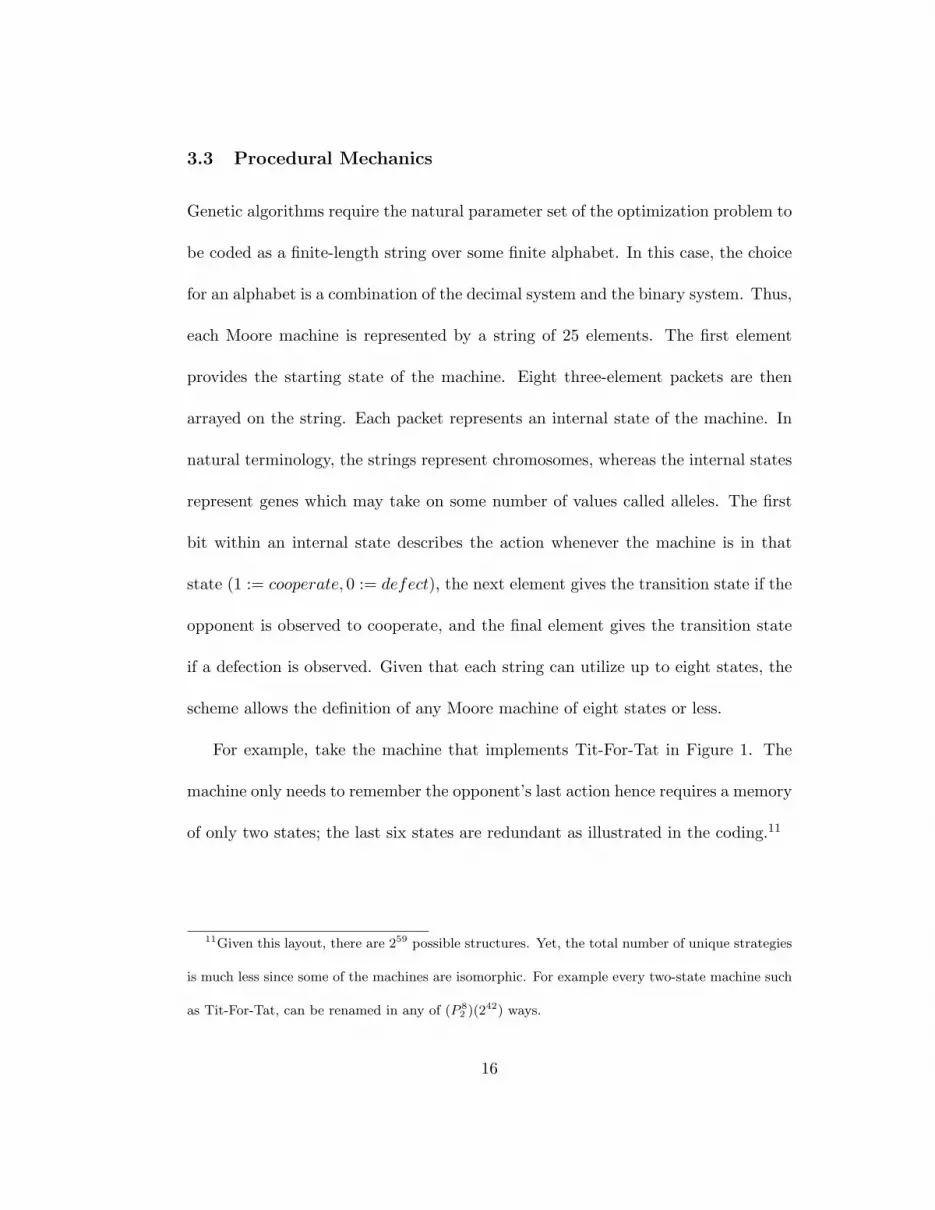
For example, take the machine that implements Tit-For-Tat in Figure 1. The
machine only needs to remember the opponent’s last action hence requires a memory
of only two states; the last six states are redundant as illustrated in the coding.11
11Given this layout, there are 259 possible structures. Yet, the total number of unique strategies
is much less since some of the machines are isomorphic. For example every two-state machine such
as Tit-For-Tat, can be renamed in any of (P 82 )(242) ways.
16

C D
D
C
start C D
Figure 1: Tit-For-Tat machine
0︸︷︷︸initial state
1 0 1︸ ︷︷ ︸state 0
0 0 1︸ ︷︷ ︸state 1
0 0 0︸ ︷︷ ︸state 2
0 0 0︸ ︷︷ ︸state 3
0 0 0︸ ︷︷ ︸state 4
0 0 0︸ ︷︷ ︸state 5
0 0 0︸ ︷︷ ︸state 6
0 0 0︸ ︷︷ ︸state 7
The genetic algorithm thus operates with a population of machines. Each ma-
chine represents an agent’s strategy. Initially a population of thirty machines is
chosen at random.12 Then, each machine is tested against the environment (which
is composed of the other machines and its twin). The encounters occur with a con-
tinuation probability of δ = 0.995 for an expected 200 periods per match. Each
machine, thus aggregates a raw score based on the payoffs illustrated in Table 1.
These scores are normalized according to the function,
x̂i =(xi − x̄)
s+ α (2)
where xi is the machine’s raw score, x̄ is the sample mean, s is the sample
standard deviation and the parameter α is chosen to be 2. Any normalized score
that is negative is truncated to zero. The choice of α implies that the machines which
do worse than two standard deviations from the mean are not allowed to be selected12The site random.org was used to generate the random numbers used in the process.
17

in the next generation. The adjusted normalized scores are thus re-normalized
to determine the probabilities of selection. Given the re-normalized scores, a new
generation of machines is chosen by allowing the top twenty performers to go directly
into the next generation.
Ten new structures are then created via a process of selection and mutation. The
process requires the draw of ten pairs of machines from the old population (with the
probabilities biased by their re-normalized scores) and the selection of the better
performer from each pair. On the other hand, mutation occurs when an element at
a random location on the selected string changes values. Each element on the string
is subjected to a 4% independent chance of mutation which implies an expectation
of 1 element-mutation per string.13 The population is iterated for 500 generations.14
13The effect of mutation obviously depends on the exact location on the string. The impact of
mutation ranges from a simple change in the starting state (even this could have a large impact, if
previously inaccessible states become active) to a more radical recombination of states.14The code was compiled and ran in Fortran.
18

4 Results
In order to investigate the impact of errors on the agents’ machines, several compu-
tational experiments are conducted. In the first set of computational experiments,
the machines are subjected to a constant independent chance of implementation
and perception errors of 4% (4%N), 2% (2%N), 1% (1%N) and 0.5% (0.5%N),
respectively. In the second set, the errors are affected by an on-off switch. When
the switch is on, the machines are subjected to a 4% independent chance of im-
plementation and perception errors, whereas when the switch is off the machines
have perfect informational accuracy. More specifically, in the NFN computational
condition, the agents’ machines are subjected to a 4% independent chance of im-
plementation and perception errors for the first 250 generations but are perfectly
transmitted and implemented for the last 250 generations. On the other hand in
the FNN condition, the machines are subjected to the 4% independent chance of
implementation and perception errors for the last 250 generations, whereas in the
first 250 generations the machines are error-free. Finally in the last set of computa-
tional experiments, the machines are subjected to a φe−ψg exponential decay (DN)
in both types of errors where φ, ψ are parameters, and g is the generation number.
The idea is that as agents become more adaptive to the environment, so does their
expertise on playing the game. The DN case is contrasted to the case where the
machines are error-free (0%N) for the entire evolution.
To assess the results of the computational experiments, it is necessary to use
19

some summary measures of machine behavior. The first summary measure is the
size of the machine, which is given by its number of accessible states. A state is
accessible if, given the machine’s starting state, there is some possible combination
of the opponent’s possible actions that will result in a transition in that state.
Therefore, even though all machines are defined on eight states, some of these states
can never be reached. Furthermore, to facilitate a better understanding of the
underlying operating mechanisms of the machines and the generation-to-generation
transitions, the Hamming distance is calculated. Formally, the Hamming distance
is defined as the number of positions between two strings of length n, for which the
corresponding elements are different. This metric will identify how heterogeneous
the population of machines is under each computational condition, and how fast the
evolved population of machines converges to some common structure.
Another summary measure that sheds more light to the machine-composition, is
the cooperation-reciprocity and the defection-reciprocity. The cooperation-reciprocity
is the proportion of accessible states that respond to an observed cooperation by the
opponent with a cooperation. On the other hand, the defection-reciprocity is the
proportion of accessible states that respond to an observed defection by the opponent
with a defection. The results that follow present the averages over all thirty members
of each generation and forty simulations15 conducted for each experiment.16 Unless15The sample sizes are large enough for an application of the Central Limit Theorem.16A variety of sensitivity analyses have been performed and they confirm that the results reported
here are robust to reasonable changes in these choices.
20

otherwise noted, to establish statistical significance the paired-differences test was
used at a 95% level of significance.
4.1 Evolution Of Payoffs & Automaton Characteristics
1
1.2
1.4
1.6
1.8
2
2.2
2.4
2.6
2.8
3
1 84 167 250 333 416 499
Generation
Averag
e P
ayo
ff
4%N 2%N 1%N 0.5%N
Figure 2: Average Payoff under 4%N , 2%N , 1%N & 0.5%N
Figure 2 shows the average payoff per game-generation over all thirty members
under the 4%N , 2%N , 1%N and 0.5%N conditions. In the early generations, the
agents tend to use machines that defect continuously. This is due to the random
generation of the machines at the start of the evolution. In such an environment,
the best strategy is to always defect. With the lapse of a few generations though,
some machines may achieve consistent cooperation, which allows the payoffs to move
21

higher. In the 4%N condition, the average payoff in the last generation is 1.44 utils
whereas in the 2%N condition, the average payoff in the last generation is 1.95 utils.
The average payoff in the 1% and 0.5% conditions in the last generation is 2.54 and
2.65 utils, respectively. The one-tailed-paired-differences test establishes that the
means of the conditions are statistically different. The results indicate that the
incorporation of errors may alter the evolution of cooperative machines and result
in non-cooperative ones instead.
0
1
2
3
4
5
6
7
8
9
10
11
12
13
14
15
16
17
18
1 84 167 250 333 416 499
Generation
Ham
min
g D
ista
nce
4
4.5
5
5.5
6
6.5
1 84 167 250 333 416 499
Generation
Averag
e N
um
ber O
f A
ccessib
le S
tate
s
4%N
2%N
1%N
0.5%N
Figure 3: Accessible States & Hamming Distance under 4%N , 2%N , 1%N & 0.5%N
The average number of accessible states per game-generation is shown on the left-
hand side of Figure 3. In the first generation, the number of accessible states of the
(randomly-chosen) machines in all four conditions, is around 6.20 out of a possible
8 states. On the other hand, in the last generation the average number of accessible
states is 4.92, 5.36, 5.72 and 5.95 in the 4%N , 2%N , 1%N and 0.5%N conditions,
respectively. The average number of accessible states is almost consistently less
22

in the noisier environments. The one-tailed-paired-differences test performed on
the number of accessible states, establishes that the means of the conditions are
statistically different. This suggests that under more noisy conditions, the average
number of accessible states drops.
A possible conclusion is that strategic simplification is advantageous in the pres-
ence of errors (if the number of accessible states is assumed to be a good measure of
complexity). In the presence of errors, behavior is governed by mechanisms that re-
strict the flexibility to choose potential actions, or that produce a selective alertness
to information that might prompt particular actions to be chosen. These mecha-
nisms simplify behavior to less complex patterns, which are easier for an observer to
recognize and predict. In the absence of errors, the behavior of perfectly informed
agents responding with flexibility to every perturbation in their environment would
not produce easily recognizable patterns, but rather would be extremely difficult to
predict.17
Furthermore, on the right-hand side of Figure 3, the Hamming distance of the
4%N , 2%N , 1%N and 0.5%N conditions is presented. The Hamming distance of the17Consider Rubic’s Cube. There are over 43 trillion possible initial positions from which to un-
scramble the cube. Minimizing the number of moves to solve the cube would require an extremely
complex pattern of adjustment from one particular scrambled position to another. Yet, if mistakes
are made in trying to select a shortcut, the cube may remain unscrambled indefinitely. Conse-
quently, cube experts have developed rigidly-structured-solving procedures that employ a small
repertoire of solving patterns to unscramble the cube. These procedures follow a predetermined
hierarchical sequence that is largely independent of the initial scrambled position.
23

4%N and 2%N conditions, settles around 0.50 positions and 1.80 positions respec-
tively, quite early. In the last generation, the Hamming distance is 0.54 positions for
the 4%N condition and 1.40 positions for the 2%N condition. On the other hand,
the 1%N and 0.5%N conditions take more time to settle at a value. By the end
of the evolution, the 1%N and 0.5%N conditions seem to settle around 2.90 and
3.60 positions, respectively. In the last generation, the Hamming distance is 2.80
positions for the 1%N condition and 3.30 positions for the 0.5%N condition. The
results suggest that in noisier environments, the evolutionary process will single out
the structure that performs well quite early, and the generations that come after,
will be composed of variants (or even clones, if mutation turns out to be innocuous)
of that particular structure. On the other hand, in the low noise-level conditions,
the population of machines is more heterogeneous and takes quite a bit of time to
settle to a particular structure.
On the left-hand side of Figure 4, the average cooperation-reciprocity per gen-
eration is shown. As errors increase, the machines tend to reduce their cooperation-
reciprocity. This observation also accounts for the low payoffs of Figure 2. In the
last generation, the proportion of states returning cooperation with an opponent’s
cooperation is 0.16, 0.27, 0.31 and 0.29 for the 4%N , 2%N , 1%N and 0.5%N con-
ditions, respectively. The one-tailed-paired-differences test performed, establishes
that the means of the conditions are statistically different. On the right-hand side,
the defection-reciprocity for the four conditions is shown. Machines in general,
24

0
0.1
0.2
0.3
0.4
0.5
0.6
1 84 167 250 333 416 499
Generation
Pro
po
rti
on 4%N
2%N
1%N
0.5%
0.5
0.6
0.7
0.8
0.9
1
1 84 167 250 333 416 499
Generation
Pro
po
rti
on
Figure 4: Cooperation-Reciprocity & Defection-Reciprocity under 4%N , 2%N ,
1%N & 0.5%N
are more likely to reciprocate a defection by the opponent with a defection, than
to cooperate after the opponent cooperates. The general pattern deduced, is that
defection is not tolerated in noisier environments. In the last generation, the propor-
tion of states returning defection with an opponent’s defection is 0.91, 0.83, 0.76 and
0.77 for the 4%N , 2%N , 1%N and 0.5%N conditions, respectively. The one-tailed-
paired-differences test establishes that the means of the conditions are statistically
different.
Figure 5 shows the average payoff per game-generation over all thirty members
under the NFN and FNN conditions. In the latter condition, the agents’ machines
are very cooperative in the beginning, maintaining a payoff mostly above 2.70 utils
until the switch occurs. In the last generation prior to the switch, the average payoff
is 2.77 utils, while in the very next generation the payoff plummets to 1.85 utils and
25

1
1.2
1.4
1.6
1.8
2
2.2
2.4
2.6
2.8
3
1 84 167 250 333 416 499
Generation
Averag
e P
ayo
ff
NFN FNN
Figure 5: Average Payoff under NFN & FNN
then gradually moves down to 1.51 utils in the last generation. The drop of almost 1
util at the switch, is not surprising; the machines evolved in the first 250 generations
are naturally, not very adaptive to the new environment established after the switch;
thus perform poorly. On the other hand, under the NFN condition, the change in
the payoffs at the switch is more gradual. In the last generation before the switch,
the average payoff is 1.34 utils while in the very next generation the average payoff is
1.37 utils. Once noise ceases, the machines are able to build some cooperation that
gradually proliferates in the following generations, resulting to an average payoff of
2.72 utils in the last generation.18
18A fundamental deviation between the two conditions, is the difference in the slopes as indicatedin the Figure. The slope of the FNN condition in the beginning, is very steep (the regression
26

0
1
2
3
4
5
6
7
8
9
10
11
12
13
14
15
16
17
18
1 84 167 250 333 416 499
Generation
Ham
min
g D
ista
nce
4
4.5
5
5.5
6
6.5
1 84 167 250 333 416 499
Generation
Averag
e N
um
ber O
f A
ccessib
le S
tate
s
NFN
FNN
Figure 6: Accessible States & Hamming Distance under NFN & FNN
The average number of accessible states per generation is shown on the left-hand
side of Figure 6. The two conditions exhibit different paths in the sense that the
average number of accessible states in the NFN condition is low in the beginning
and then once the switch takes place increases, whereas in the FNN condition, the
average number of accessible states starts high and then after the switch, declines.
coefficient indicates that the payoff rises by approximately 0.57 utils every 10 generations). On the
other hand, the slope of the NFN condition is less steep (in this case, the regression coefficient
indicates that the payoff rises by approximately 0.13 utils every 10 generations). The proportion
of accessible states that respond to an observed cooperation by the opponent with defection, is
1− cooperation-reciprocity. In the beginning of the FNN condition, the proportion of accessible
states that respond to an observed cooperation with defection is 0.7. On the other hand, in the
NFN condition after the lapse of 250 generations, the proportion of states that respond to an
observed cooperation with defection is 0.84 (1− 0.16). Therefore, it will take more time to evolve
cooperative machines in the latter condition which ultimately explains the difference in the slopes
of the two conditions.
27

The final value in the NFN condition is 5.92 accessible states whereas the final value
in the FNN condition is 4.89 accessible states. Furthermore, the Hamming distance
is presented on the right-hand side. In the NFN condition, the population just
before the switch averages 0.63 positions which steadily goes up to 5.05 positions,
before settling at 4.15 positions in the last generation. On the other hand, the
Hamming distance in the FNN condition is 7.18 positions just before the switch
and goes down to 0.53 positions in the last generation.
Figure 7 (left-hand side) shows the average cooperation-reciprocity in the NFN
and FNN conditions. In the latter condition, the cooperation-reciprocity peaks
around the 60th generation at 0.54 but then gradually declines reaching a low of
0.22 in the last generation. On the other hand, the cooperation-reciprocity in the
NFN condition is over 0.15 but less than 0.2 for the first 250 generations. After
the switch, the cooperation-reciprocity steadily increases reaching 0.52 in the last
generation. The paired-differences in the means are statistically significant. On
the right-hand side, the average defection-reciprocity per game-generation is shown.
The NFN operates at essentially two levels; the one level is around 0.90 and lasts for
the generations prior to the switch and the second level is around 0.78 and lasts for
the final 150 generations. On the other hand, in the FNN condition, the increase in
the defection-reciprocity is gradual with the exception of a short transitioning period
after the switch takes place. In the last generation, the defection-reciprocity of the
NFN condition is 0.77 whereas the defection-reciprocity of the FNN condition is
28

0.89. The paired-differences in the means are statistically significant.
0
0.1
0.2
0.3
0.4
0.5
0.6
1 84 167 250 333 416 499
Generation
Pro
po
rti
on
NFN
FNN
0.5
0.6
0.7
0.8
0.9
1
1 84 167 250 333 416 499
Generation
Pro
po
rti
on
Figure 7: Cooperation-Reciprocity & Defection-Reciprocity under NFN & FNN
Figure 8 shows the average payoff per game-generation over all thirty members in
the DN and 0%N conditions. The exponential-decay-over-time is calculated by the
formula φe−ψg where φ, ψ are parameters, and g is the generation number.19 The
secondary axis, indicates the probability of implementation and perception errors as
a percentage evolved over time. In the DN condition, the average payoff increases
steadily (up to an upper bound) given the set parameters of the exponential decay
function. The dotted line indicates that the rise (from the 75th upto the 350th
generation) is almost-linear. The regression coefficient calculated for the dotted line
increases by approximately 0.14 utils every 10 generations. The average payoff is19In the computations, φ = 0.04 and ψ = 0.01. The choice of parameters reflect an initial 4%
probability of implementation and perception errors that exponentially decays reaching some ε %
probability by the end of the evolution for ε > 0.
29

2.24 utils after 250 generations and 2.77 utils in the last generation. On the other
hand, after the initial decline in the first six generations, the 0%N condition seems
to settle around 2.8 utils. In the last generation, the average payoff of the 0%N
condition is 2.85 utils.
1
1.2
1.4
1.6
1.8
2
2.2
2.4
2.6
2.8
3
1 84 167 250 333 416 499
Generation
Averag
e P
ayo
ff
0
0.5
1
1.5
2
2.5
3
3.5
4
0%N DN NL
Figure 8: Average Payoff under O%N & DN
Figure 9 (left-hand side) shows the average number of accessible states. The
exponential decay condition exhibits an increase in the average number of accessible
states as the noise level decays. Furthermore, in the last generation the average
number of accessible states is 5.98. On the other hand, in the 0%N condition
the average number of accessible states seems to settle quite fast at around 6.15
30

0
1
2
3
4
5
6
7
8
9
10
11
12
13
14
15
16
17
18
1 84 167 250 333 416 499
Generation
Ham
min
g D
ista
nce
4
4.5
5
5.5
6
6.5
1 84 167 250 333 416 499
Generation
Averag
e N
um
ber O
f A
ccessib
le S
tate
s
0%N
DN
Figure 9: Accessible States & Hamming Distance under O%N & DN
accessible states. The one-tailed-paired-differences test establishes that the means
of the conditions are statistically different. On the right-hand side of Figure 9, the
Hamming distance of the two conditions is presented. The Hamming distance in the
0%N condition fluctuates quite a bit, reaching 4.24 positions in the last generation.
This is indicative of the presence of heterogeneous machines within the population
for a substantial amount of time. On the other hand, the population in the DN
condition, is less heterogeneous stabilizing around 3.65 positions by the end of the
evolution. In the last generation, the Hamming distance in the DN condition is
3.52 positions.
Figure 10 (left-hand side) shows the average cooperation-reciprocity per genera-
tion over all thirty machines. The average cooperation-reciprocity in the 0%N con-
dition, fluctuates around 0.50 after the initial 35 generations. In the last generation,
31
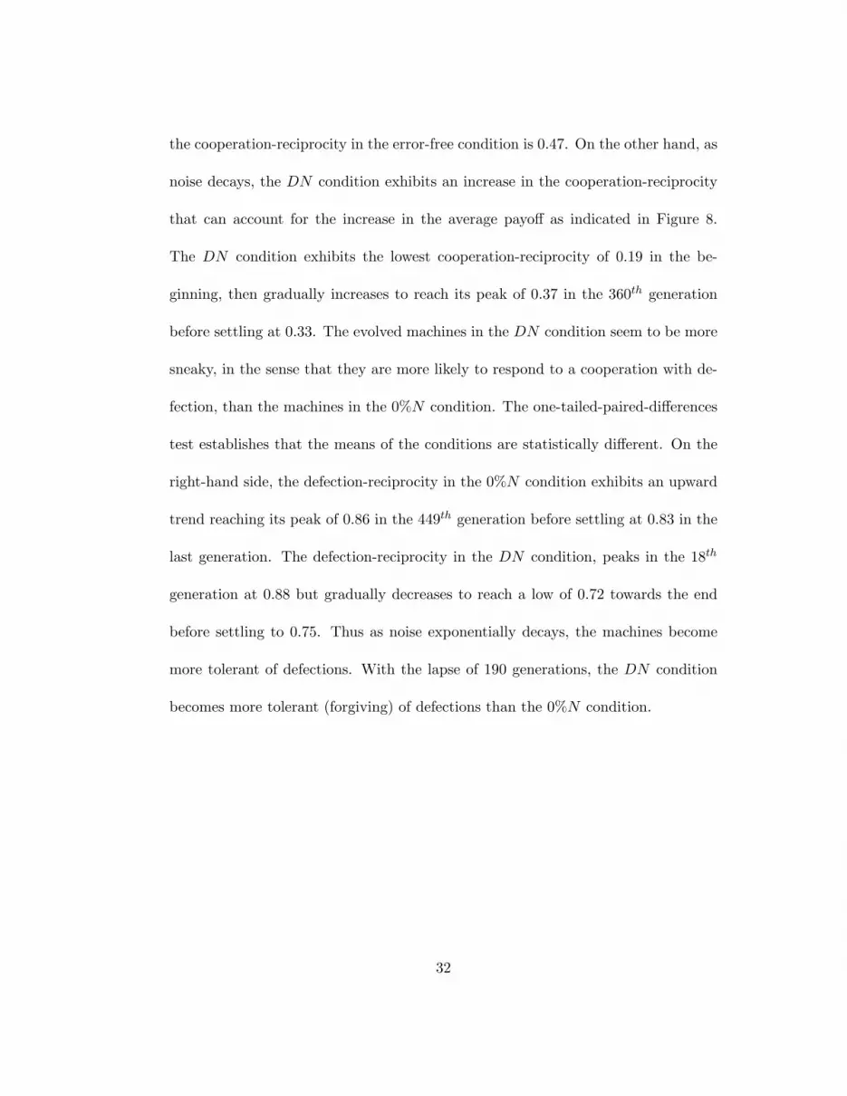
the cooperation-reciprocity in the error-free condition is 0.47. On the other hand, as
noise decays, the DN condition exhibits an increase in the cooperation-reciprocity
that can account for the increase in the average payoff as indicated in Figure 8.
The DN condition exhibits the lowest cooperation-reciprocity of 0.19 in the be-
ginning, then gradually increases to reach its peak of 0.37 in the 360th generation
before settling at 0.33. The evolved machines in the DN condition seem to be more
sneaky, in the sense that they are more likely to respond to a cooperation with de-
fection, than the machines in the 0%N condition. The one-tailed-paired-differences
test establishes that the means of the conditions are statistically different. On the
right-hand side, the defection-reciprocity in the 0%N condition exhibits an upward
trend reaching its peak of 0.86 in the 449th generation before settling at 0.83 in the
last generation. The defection-reciprocity in the DN condition, peaks in the 18th
generation at 0.88 but gradually decreases to reach a low of 0.72 towards the end
before settling to 0.75. Thus as noise exponentially decays, the machines become
more tolerant of defections. With the lapse of 190 generations, the DN condition
becomes more tolerant (forgiving) of defections than the 0%N condition.
32

0
0.1
0.2
0.3
0.4
0.5
0.6
1 84 167 250 333 416 499
Generation
Pro
po
rti
on
0%N
DN
0.5
0.6
0.7
0.8
0.9
1
1 84 167 250 333 416 499
Generation
Pro
po
rti
on
Figure 10: Cooperation-Reciprocity & Defection-Reciprocity under O%N & DN
4.2 Prevailing Structures
The results of the previous section are indicative of the mechanics of the evolving
machines. Yet, it is imperative to also examine the prevailing structures in all fic-
titious environments. This way, a lot can be said about the type of machines that
survive or even the type of machines that do not survive in these environments.
Therefore, in what follows, the prevailing structure of each computational condition
is discerned by deriving the distribution of prevailing machines over the forty simu-
lations. To that end, Figure 11 shows the frequency distribution of each condition.
Given the convergence of the population of machines by the last generation, it is un-
necessary to incorporate the entire last-generation population into the distribution.
Instead, the best performer from each simulation is picked, for a total frequency of
forty machines for each condition. The horizontal axis of the frequency distributions
in Figure 11, provides the names of the structures which correspond to the Moore
33

machines in Figure 12.
Distribution under NFN Distribution under FNN
Distribution under DN Distribution under 0%N
Distribution under 4%N Distribution under 2%N
Distribution under 1%N Distribution under 0.5%N
0
5
10
15
20
M1 M2 M4 Other
Freq
uen
cy
0
5
10
15
20
M4 M5 M6 Other
Freq
uen
cy
0
5
10
15
20
M6 M7 M8 Other
Freq
uen
cy
0
5
10
15
20
M6 M7 M8 Other
Freq
uen
cy
0
5
10
15
20
M1 M2 M3 Other
Freq
uen
cy
0
5
10
15
20
M1 M4 M5 Other
Freq
uen
cy
0
5
10
15
20
M4 M1 M6 Other
Freq
uen
cy
0
5
10
15
20
M4 M5 M6 Other
Freq
uen
cy
Figure 11: Frequency Distributions
34

M1 M2C,D C,D
C,D C,D C,D C,D
M3 C
D
C,D C,D C,D C,D
M4D C
C
D C,D C,D C,D
M5C
C C D C
D D D C,D C,D
M6C D
C C
D D C,D C,D C,D
M7C C
C D
D D C,D C,D C,D
M8C C
C D
D D C,D C,D C,D C,D
start
start
start
start
start start
start
start
D C D D DD
C D DDD
C D D DD
C DD DDC
C DD DDC
C DD DDC
C DD DDC D
Figure 12: Moore Machines
The prevailing Moore machine of each condition, is presented below. Since some
conditions share identical prevailing structures, it is only appropriate to group these
conditions together. For example, the 4%N condition and the FNN condition
share the same prevailing structure. On the other hand, the 2%N condition has a
35

prevailing structure that is different from all other conditions. The 1%N , 0.5%N
and the DN conditions share the same prevailing structure, and so do the 0%N and
the NFN conditions.
C,D
C,D C,D C,D C,Dstart
C D D DD
Figure 13: Prevailing Machine under 4%N & FNN
The prevailing structure of the 4%N condition and the FNN condition is com-
posed of five accessible states as shown in Figure 13. The machine is open-loop. In
other words, the actions taken at any time-period only depend on that time-period
and not, on the actions of the opponent (this is a history-independent machine).
In the first period, the machine cooperates but then counts four defections before
cooperating again. The expected payoff per period of such a machine in a popula-
tion composed of clones (without errors) is 1.40 utils. The cooperation-reciprocity
is 0.20 while the defection-reciprocity is 0.80.
D C
C
D C,D C,D C,Dstart
C D D DD
Figure 14: Prevailing Machine under 2%N
36

The prevailing structure of the 2%N condition is also composed of five accessible
states. Contrary to the previous structure, this one is a closed-loop machine where
the actions in any time-period depend on the history of play. The machine is similar
to the one in Figure 13 with some notable transition-differences. The cooperating
state has a loop on itself in case the opponent is observed to cooperate; an indication
of appreciation of cooperative play. Yet, if the opponent chooses to defect, the
machine will punish the opponent with at least four defections before returning to
the cooperating state again. In addition, the machine incorporates a sneaky state
which tries to exploit machines that enter cooperative modes earlier.
C
C D C
D D C,D C,D C,Dstart C DD DDC
Figure 15: Prevailing Machine under 1%N , 0.5%N & DN
On the other hand, the prevailing structure of the 1%N condition, 0.5%N con-
dition and DN condition is composed of six accessible states as shown in Figure
15. This machine is again a closed-loop machine where the actions are contingent
on the history of play. Furthermore, the machine is quite rich in the sense that
it incorporates a lot of notions. It consists of a combination of Two-Tits-For-Tat,
mingled with at least four periods of punishment in case of non-comformity to the
37

cooperative outcome. In addition, just like the previous structure, it contains a
sneaky state that tries to exploit machines that enter a cooperative mode earlier.
The cooperation-reciprocity of this structure is 0.33 while the defection-reciprocity
is 0.67.
C C
C D
D D C,D C,D C,Dstart C DD DDC
Figure 16: Prevailing Machine under 0%N & NFN
The prevailing structure of the 0%N condition and NFN condition is composed
of six accessible states as shown in Figure 16. This closed-loop machine is again a
combination of Two-Tits-For-Tat with at least four periods of punishment in case
of non-comformity to the cooperative outcome. The sneaky state is replaced with
a non-tolerant one, mandating that the opponent cooperates before going back to
the cooperating states. The cooperation-reciprocity in this structure is 0.50 and the
defection-reciprocity is 0.83.
A common trait in these prevailing structures, is that they contain more de-
fecting states than cooperating states; yet, in the last three structures there exists
an inherent pursue towards establishing some consistent cooperation. In a different
case, the machines will react by punishing the opponent for at least four periods
before making an effort to revisit the cooperating state(s). Furthermore, the pre-
vailing structures do not contain any terminal states. A terminal state is one that
38

has transitions only to itself; that is, once a terminal state is reached, the machine
remains in the state for the remainder of the game. Thus, machines executing strate-
gies such as Grim-Trigger do not survive in such an evolving environment for the
conditions investigated.
39

5 Conclusion
Via an explicit evolutionary process simulated by a genetic algorithm, I indicate
that the incorporation of bounded rationality in the form of action-implementation
and perception errors in the agents’ machines, is sufficient to alter the evolution of
cooperative machines and result in non-cooperative ones instead. Under the first
set of computational experiments, the evolved machines are highly non-cooperative
when the error-levels are high, but cooperative when the error-levels are low. On the
other hand, in the second and third sets of computational experiments, the machines
are non-cooperative (with the exception of the 0%N) as long as the errors persist,
but once the errors decrease or cease, the machines become more cooperative.
Furthermore, the machines exhibit some interesting characteristics in the pres-
ence of errors which lead to the conclusion that the structure as well as the magnitude
of the error-level in this environment, is quite important. If the number of accessible
states is a good measure of complexity, then a possible conclusion from the computa-
tions, is that strategic simplification is advantageous in the presence of errors. Also,
as errors persist, machines become less prone to return cooperation to an observed
cooperation. On the other hand, the defection-reciprocity indicates that machines
in noisy environments have low tolerance to defections. The latter observations are
reflected in the low payoffs of the machines in the presence of errors. In addition,
the Hamming distance indicates that the agents’ machines converge faster to some
prevailing structure as the likelihood of errors increases.
40

The prevailing structures of the computational conditions sketched in the previ-
ous section, highlight the presence of more defecting than cooperating states, with
the understanding that the cooperating states are meant to establish some consistent
mutual cooperation, whereas the defecting states are meant as punishment-counters
imposing at least four-period defections, in case of non-conformity to the coopera-
tive outcome by the opponent. Finally, in the presence of (as low as) 4% likelihood
of errors, open-loop machines (independent of the history of play) emerge endoge-
nously. The latter, cooperate for one period and defect for the next four periods
without paying any consideration to the game-plan of the opponent.
A wide variety of potential extensions exist. In this study, it was assumed that
all machines were subjected to the same level of noise, generation by generation.
Instead, the level of noise could be contingent upon the number of states accessed by
the particular machine. The rationale is that a machine that contains only one state
(say, Always Cooperate), is less likely to commit errors than one, that is far more
complex. Furthermore, it would be interesting to examine whether the results are
robust to the symmetry of the payoffs. One of the basic features of the conventional
Prisoner’s Dilemma stage-game is the requirement that the values assigned to the
game are the same for both agents. Not uncommon however, are social transactions
where not only is each agent’s outcome dependent upon the choices of the other,
but also where the resources and therefore possible rewards, of one agent exceed
41

those of the other. A social interaction characterized by a disparity in resources and
potentially larger rewards for one of the two participants would in all likelihood call
into play questions of inequality. Thus, one could run two co-evolving populations
with asymmetric payoffs, to see how inequality comes into play and in particular,
how the asymmetry in payoffs affects cooperation under the examined error-level
structures.
42

6 Appendix
A finite automaton is a mathematical model of a system with discrete inputs and
outputs. The system can be in any one of a finite number of internal configurations
or “states”. The specific type of finite automaton used here is a Moore machine.
A Moore machine20 for an adaptive agent i in an infinitely-repeated game of G =
(I,{Ai}i∈I , {gi}i∈I),21 is a four-tuple (Qi, qi0, f i, τ i) where Qi is a finite set of
internal states, of which qi0 is specified to be the initial state, f i : Qi → Ai is an
output function that assigns an action to every state, and τ i : Qi×A−i → Qi is the
transition function that assigns a state to every two-tuple of state and other agent’s
action.22
In the first period, the state is qi0 and the machine chooses the action f i(qi0).
20A Mealy machine is another type of finite automaton. Mealy machines share the same charac-
teristics with Moore machines with the exception of the output function that maps both the state
and the input to an action. However, it can be shown that the two types are equivalent hence the
analysis does not preclude Mealy machines.21I is the set of players, Ai is the set of i’s actions, and gi : A → R is the real-valued utility
function of i.22Note that the transition function depends only on the present state and the other agent’s action.
This formalization fits the natural description of a strategy as agent i’s plan of action in all possible
circumstances that are consistent with agent i’s plans. In contrast, the notion of a game theoretic
strategy for agent i requires the specification of an action for every possible history, including those
that are inconsistent with agent i’s plan of action. To formulate the game theoretic strategy, the
only change required would be to construct the transition function such that τ i : Qi × A → Qi
instead of τ i : Qi ×A−i → Qi.
43

If a−i is the action chosen by the other agent in the first period, then the state of
agent i’s machine changes to τ i(qi0, a−i) and in the second period agent i chooses the
action dictated by f i in that state. Then, the state changes again according to the
transition function, given the other agent’s action. Thus, whenever the machine is
in some state q, it chooses the action f i(q) while the transition function τ i, specifies
the machine’s transition from q (to a state) in response to the action taken by the
other agent.
For example, the machine (Qi, qi0, f i, τ i) in Figure 17, carries out the Grim-
Trigger strategy that chooses C so long as both agents have chosen C in every period
in the past, and chooses D otherwise. In the transition diagram, the vertices denote
the internal states of the machine and the arcs labeled with the action of the other
agent, indicate the transition to the states.
C C,D
Dstart C D
Figure 17: Grim-Trigger machine
Qi = {qC , qD}
qi0 = qC
f i(qC) = C and f i(qD) = D
τ i(q, a−i) = {qC (q,a−i)=(qC ,C)qD otherwise
44

References
[1] Axelrod, R. (1980). “Effective Choice in the Prisoner’s Dilemma,” Journal Of
Conflict Resolution 24, 3-25.
[2] Axelrod, R. (1980). “More Effective Choice in the Prisoner’s Dilemma,” Journal
Of Conflict Resolution 24, 379-403.
[3] Axelrod, R. and Hamilton, W. D.(1981). “The Evolution of Cooperation,” Sci-
ence 211, 1390-1398.
[4] Axelrod, R. (1984). The Evolution of Cooperation, Basic Books: New York.
[5] Flood, Merrill M. (1952). “Some Experimental Games,” Research Memorandum
RM-789, Santa Monica, California: RAND Corporation.
[6] Goldberg, D. (1989). Genetic Algorithms in Search, Optimization, and Machine
Learning, Addison-Wesley Publishing Company.
[7] Holland, J. (1975). Adaptation in Natural and Artificial Systems, MIT Press.
[8] Miller, J. (1996). “The Coevolution of Automata in the Repeated Prisoner’s
Dilemma,” Journal Of Economic Behavior & Organization 29, 87-112.
[9] Moore, E. (1956).“Gedanken Experiments on Sequential Machines,” in Au-
tomata Studies, Princeton, New Jersey: Princeton University Press.
[10] Rubinstein, A. (1986). “Finite Automata Play the Repeated Prisoner’s
Dilemma,” Journal Of Economic Theory 39, 83-96.
45

[11] Selten, R. (1975).“A Re-examination of the Perfectness Concept for Equilibrium
Points in Extensive Games,” International Journal of Game Theory 4, 25-55.
[12] Simon, H. (1947). Administrative Behavior: A Study of Decision-Making Pro-
cesses in Administrative Organizations, The Free Press.
[13] Weibull, W. J. (2002). “What have we Learned from Evolutionary Game Theory
so Far?,” Mimeo, Stockholm School Of Economics.
46


