Download pdf - An improved masking method for absorbing boundaries in electromagnetic particle simulations

Computer Physics Communications 137 (2001) 286–299www.elsevier.nl/locate/cpc

An improved masking method for absorbing boundariesin electromagnetic particle simulations

Takayuki Umeda, Yoshiharu Omura∗, Hiroshi MatsumotoRadio Science Center for Space and Atmosphere, Kyoto University, Uji, Kyoto 611-0011, Japan

Received 11 December 2000; received in revised form 24 January 2001; accepted 26 January 2001

Abstract

We have developed a new scheme to mask electromagnetic fields for absorbing boundaries used in electromagnetic particlecodes. The conventional masking method can suppress reflection of various plasma waves by assigning large damping regionsfor absorbing boundaries. It requires substantial computer memory and processing time. We introduce two new parametersto control absorption of outgoing electromagnetic waves. The first parameter is a damping parameter to change the effectivelength of damping regions. The second parameter is a retarding parameter to change phase velocities of electromagnetic wavesin the damping regions. As a new masking method, we apply both damping and retarding factors. We also found that the bestabsorption of outgoing waves is realized with a combination of a smaller damping factor and a larger retarding factor. The newmethod allows us to reduce the size of damping regions substantially. 2001 Elsevier Science B.V. All rights reserved.

PACS: 02.70; 52.65.R

Keywords: Absorbing boundary conditions; EM PIC code

1. Introduction

In particle simulations of space plasmas, both periodic and open systems are used for studies of nonlinearwave-particle interaction in space plasmas. Periodic systems are used to simulate micro-scale phenomena suchas time evolution of infinite uniform systems. On the other hand, large-scale phenomena such as spatial evolutionof localized perturbation are studied in open systems rather than periodic systems. Open systems are regarded asone part of an infinite space. Boundary conditions of open systems are called ‘open’ or ‘free’ boundaries. Sincewe pick up a segment of real space plasmas as a ‘simulation box’, we need a special numerical treatment ofthe boundaries between the simulation box and the surrounding outer region. A requirement for open boundaryconditions is to behave as if there were no boundaries. An important problem in simulation studies in open systemsis reflection of electromagnetic waves at boundaries. There have been a number of studies on boundary conditionswhich can suppress reflection of outgoing waves (e.g., [1,2]). They are called ‘absorbing boundaries’.

* Corresponding author.E-mail addresses: [email protected] (T. Umeda), [email protected] (Y. Omura), [email protected]

(H. Matsumoto).

0010-4655/01/$ – see front matter 2001 Elsevier Science B.V. All rights reserved.PII: S0010-4655(01)00182-5

T. Umeda et al. / Computer Physics Communications 137 (2001) 286–299 287

Algorithms of absorbing boundaries fall into two categories. In the algorithms in the first category (e.g., [3,4]), boundaries are simulated by assuming that outgoing electromagnetic waves have a certain phase velocity.Scalar wave equations are solved to approximate boundary values so that outgoing waves are not reflected at theboundaries. While there are many kinds of plasma waves which have different frequencies and phase velocities,the algorithms in the first category can only absorb a single wave mode.

The algorithms in the second category are to absorb outgoing waves using a resistive medium such as a di-electric. In laboratory experiments, so called a wave absorber is located on the wall. In particle simulations, the‘masking method’ (damping region method) [5] is used. In this method, outgoing waves are artificially damped bysimple masking of electromagnetic fields in ‘damping regions’ attached at both ends of the simulation box. Whilethe masking method is a useful scheme which can suppress reflection of various plasma waves at boundaries, thismethod has the following weak point. Electromagnetic waves that propagate through a resistive layer can be com-pletely absorbed if the thickness of the layer is large enough. A larger resistive layer gives better absorption. There-fore, the absorbing boundaries in the second category requires substantial computer memory and processing time.

In the present study, we avoid the weak point of the masking method by developing an improved scheme ofthe masking method. In Section 2, we first investigate the characteristics of the conventional masking method.We introduce a new masking parameter to control effective length of damping regions. The characteristics of theimproved masking method with the effective damping regions are also investigated in this section. In Section 3,we introduce one more parameter and use two different masking factors to absorb outgoing waves. We also try toobtain the most effective combination of the two masking factors. Section 4 gives summary and conclusion.

2. Effective damping region

In the present study, we used Kyoto university one-dimensional ElectroMagnetic Particle cOde (KEMPO1) [6].The masking method is adopted in KEMPO for about two decades because it is easily implement in the simulationcode. The simulation model is schematically illustrated in Fig. 1. The simulation system is taken along thex-axis.The system consists of a physical region and damping regions. The damping regions are attached at both ends of thephysical region. The external (static) magnetic fieldB0 is taken in thex–y plane. The amplitude ofB0 is given by

B0x = Ωe

(q/me)cosθ

B0y = Ωe

(q/me)sinθ

(1)

Fig. 1. Simulation model. Electromagnetic waves are radiated at the center of the simulation system and absorbed in the damping regions.

288 T. Umeda et al. / Computer Physics Communications 137 (2001) 286–299

whereΩe, q/me andθ are electron cyclotron frequency, electron charge-to-mass ratio and the angle betweenB0

and thex-axis, respectively. We assume a current source at the center of the simulation system. The external currentJ0 is driven in thez-direction and electromagnetic waves are radiated in the system. The currentJ0 is given by

J0 =AJ sin(ωJ t) for 0 t 2π/ωJ ,

0 for t > 2π/ωJ ,(2)

whereAJ andωJ are the amplitude and frequency, respectively. As the initial condition, all electrons in the systemform a Maxwellian velocity distribution given by

f (v)= N√2πVth

exp

(− v2

2V 2th

), (3)

whereN andVth are density and thermal velocity, respectively. Ions are assumed to be uniform neutralizing back-ground with an infinite mass in the simulation system. The common parameters for all simulation runs are listedbelow.

Grid spacing x · ωJ /c= 0.02;Time step ωJt = 0.016;Length of physical region L · ωJ /c= 20.48;Debye length λD · ωJ /c= 0.02;

whereλD = Vth/Πe. These values are normalized by the frequency of the driving currentωJ and the light speedc.We use 1024 superparticles for one grid point.

We generate three type of plasma waves varying electron plasma frequencyΠe, electron cyclotron frequencyΩe and θ . The parameters for the three modes are listed in Table 1. Run (a) corresponds to light mode, i.e.electromagnetic waves in vacuum. Whistler mode andX-mode waves are excited is runs (b) and (c), respectively,as indicated by their dispersion relations shown in Fig. 2.

Outgoing waves are absorbed by simple masking electromagnetic fields in the damping regions. In other words,their amplitude are gradually reduced by multiplying a masking functionfM to the right-hand side of the timedifference form of Maxwell’s equations at each time step, written as,

B t+t/2(x)= Bt−t/2(x)−t(∇ × Et (x))

·fM(x)

Et+t/2(x)= Et−t/2(x)−t(J t (x)− c2∇ × B t (x))

·fM(x)

(4)

Table 1Simulation parameters varied for different runs

Run Πe/ωJ Ωe/ωJ θ

(a) 0.0 0.0 0

(b) 10.0 10.0 0

(c) 2.0 8.0 90

ωJ is the frequency of the driving current.


Fig. 2. Dispersion relation of run (b) (left) and run (c) (right) in Table 1. The dashed lines show the parameter of simulation runs. Whistler modeandX-mode waves are generated from the parameter run (b) and (c), respectively.

Fig. 3. Masking function and procedure of the masking method.L andLD represent lengths of the physical and damping regions, respectively.

We use a parabolic masking function withfM = 1 in physical region andfM < 1 in damping regions.fM varygradually from 1 to smaller value closer to the boundary. The masking function and procedure of the maskingmethod are schematically illustrated in Fig. 3. The masking function is given by

fM(x, r)= 1 for |x| L

2 ,

1− (r

|x|−L/2LD

)2 for |x|> L2 ,

(5)

whereLD (=NDx) represents length of damping regions. We introduce a new masking parameterr (0< r 1)to change the gradient of the function. The masking functionfM becomes 0 atx = ±(L/2+ LD/r). As shown inFig. 4,LD/r represents length of the ‘effective’ damping region. We define the masking parameterr by

r = Length of real damping region

Length of effective damping region. (6)

In the conventional masking method, the masking function (5) is used withr = 1.0.Firstly, we use the conventional method and change the length of the damping regionsLD to study the reflection

ratio of light mode, whistler mode andX-mode waves. As one of simulation results, we show the spatial and timeprofile of intensity of the three plasma waves forLD = 320 in Fig. 5. We compute magnetic field energy|B2

y +B2z |

at each grid point and time step. Space is normalized by the wavelength of light mode wavesλ = 2πc/ω. In thepresent study,λ= 314. Time is normalized by the frequency of external currentωJ . The intensity of magnetic fieldis normalized by amplitude of incident waves. The size of damping region is indicated by the thick lines above the


Fig. 4. Shape of the masking function (5) for differentr . The dashed and solid lines correspond tor = 1.0 andr = 0.5, respectively. Length ofthe effective damping region is given byLD/r .

Fig. 5. Spatial and time profiles of magnetic field energy,|B2|, of light mode (left), whistler mode (center),X-mode waves (right), respectively.The masking function (5) withr = 1.0 is applied to 320 grid points in each damping region. The sizes of the damping region are shown by thelines above the figures.

figures. As shown in Fig. 5, electromagnetic waves are radiated at the center of the system and propagate to theboundary. While they are absorbed in the damping regions, some waves are reflected in the damping regions.

To calculate the reflection ratio, we specify two regions in the space-time plane for incident and reflected waves,respectively, as schematically illustrated in Fig. 6. The reflection ratioΓ is given by the integration of magneticfield energy in the specified regions, as follows:

Γ = 10× log10Ireflect

Iin[dB], (7)

Iin =t0+t ′∫t0

L/4+λ/10∫L/4−λ/10

∣∣B2y +B2

z

∣∣dx dt, (8)


Fig. 6. We specify two regions in the space-time plane covering the same size of passage of incident and reflected waves, respectively. Wedefine intensity of incident and reflected waves by integration of magnetic field energy in the specified regions.L andλ represent length of thephysical region and wave length of light mode, respectively,t0 andt1 represent times when incident and reflected waves come into each pickedup region, respectively.

Fig. 7. Reflection ratio as functions of length of the damping regionLD for light mode, whistler mode andX-mode waves, respectively.λ= 314grid represents wave length of light mode. For whistler mode,Πe/Ωe = 1.0. ForX-mode,Πe/Ωe = 0.25.

Ireflect=t1+t ′∫t1

L/4+λ/10∫L/4−λ/10

∣∣B2y +B2

z

∣∣dx dt, (9)

t ′ = λ

5vg+ 2π

ωJ, (10)

wherevg is group velocity of the waves. We show the reflection ratio of three plasma waves for different lengthof the damping regions in Fig. 7. The dashed, solid and dotted line correspond to light mode, whistler mode andX-mode waves, respectively. The length of the damping regions is normalized by the wavelength of light modeλ.


Fig. 8. Reflection ratio as functions ofr in (5) for light mode, whistler mode andX-mode waves, respectively.LD = 64. Smallerr correspondsto the smaller masking factor.

The conventional masking method gives better absorption for both waves with larger damping regions, as describedin Section 1.

As shown in Fig. 5, outgoing waves penetrate only 30% of the damping regions and are reflected near theboundary between the physical region and the damping region. This implies that large part (about 70%) of thedamping region is not used for absorption of the waves. When we use a large damping region, gradient maskingfunction becomes small. Therefore, the gradient of masking function is rather important than the size of dampingregions. Since change of function value indicates change of a medium where the waves are propagating, a bettermasking function should be realized with a smaller gradient.

Next, we varying the masking parameterr and change the gradient of the masking function (5), i.e. length ofthe effective damping regions. Reflection ratio of three plasma waves for different masking factors are shown inFig. 8. We obtain minimum reflection ratio for light mode, whistler mode andX-mode withr 0.35, 0.25 and 0.3,respectively. As described above, when we use large masking factor, electromagnetic waves are reflected near theboundary between the physical region and the damping region and we cannot have good absorption. By varyingr from 1.0 to smaller value, electromagnetic waves can penetrate the damping regions deeply and reflection ratiobecomes smaller. When we use too small masking factor, reflection ratio becomes larger because electromagneticwaves can reach the boundary of the system with a finite amplitude and are reflected back into the system.

Let us consider a finite amplitude wave with the following form is propagating in damping regions.

BW(t)= BW0 exp(−iω0t). (11)

From the computation (4), time variation of waves amplitude is expressed as

∂BW

∂t= αB

t+t/2W −B

t−t/2W

t= (ωi − iωr)BW , (12)

whereα is the masking factor (equivalent tofM). From (11) and (12), we obtain the damping ratioωi as follows:

∂BW

∂t= αB

t+t/2W −B

t−t/2W

t(13)

= α exp(−i ω0t2 )− exp(i ω0t

2 )

tBW0(−iω0t) (14)

−

1− α

tcos

ω0t

2− i

1+ α

tsin

ω0t

2

BW0 exp(−iω0t), (15)


ωi = 1− α

tcos

ω0t

2. (16)

By assumingt is small enough, the damping ratio normalized by the driving frequencyω0 is given by

ωi

ω0= 1− α

ω0t. (17)

Since the amplitude variation propagates at a group velocity, the spatial damping ratioki (k = kr + iki) is given by

ki = ωi

vg= 1− α

vgt. (18)

We define an ‘effective’ spatial damping ratio in damping regions as

LD∫0

ki dx = LD

1∫0

r2x2

vgtdx = NDr

2

3vg tx, (19)

where we replaceα by 1− r2x2. vg tx represents a group velocity of waves in the simulation. We callvgtx

aneffective group velocity. We have performed simulations with various combination of size of damping regionND,the masking parameterr and the effective velocityvg tx . We found that the best masking parameterr0 satisfies thefollowing relation

NDr20

3vg tx 3.3. (20)

Effect of the masking method (reflection ratio) also depends on other values besides the effective group velocity,such as number of grid points for a damping regionND, effective frequencyωt and effective wave numberkx.From Eqs. (17) and (18), we need larger damping regions to absorb those waves whose frequency is smaller orwhose group velocity is slower.

3. Phase retardation

In this section, we introduce another masking factor in Eqs. (4). We can separate the right-hand side of thetime difference form of Maxwell’s equations into two parts. The first part represents original field values, i.e.electromagnetic fields at the previous time step (at timet − t

2 ). The second (at timet) represents the incrementsof the electromagnetic fields for one time step. We use two masking parametersrd andrr , and apply the maskingfunction (5) with the different masking parameters as shown in the following form:

B t+t/2(x)= fM(x, rd) ·(B t−t/2(x)−t

(∇ × Et (x)) · fM(x, rr )

)Et+t/2(x)= fM(x, rd) ·

(Et−t/2(x)−t

(J t (x)− c2∇ × Bt (x)

) · fM(x, rr)) (21)

If rr = 0, i.e.fM(x, rr ) = 1.0, the above procedure is reduced to the method in Section 2. We analyze effect ofeach masking factor. We replace both masking functionsfM(x, rd) andfM(x, rr ) by factorsα andβ , as follows:

Bt+t/20 = Bt−t/2 − βt(∇ × Et )

Et+t/20 = Et−t/2 − βt(J t − c2∇ × B t )

(22)

B t+t/2 = αBt+t/20

Et+t/2 = αEt+t/20

(23)


Eqs. (23) show that the amplitude (energy) of outgoing waves are gradually reduced in the damping regions ateach time step. The masking factorα can be regarded as a ‘damping factor’. On the other hand, we cannot absorboutgoing waves when we applyβ assumingα = 1. In this case, we can obtain the wave equation (24) for lightmodes, as follows:

∂2E

∂t2= (β · c)2∇2E

∂2B

∂t2= (β · c)2∇2B

(0< β < 1). (24)

Eqs. (24) shows that electromagnetic waves propagate slower than the light speed with group velocityvg = β · cin damping regions. We also apply the masking factor ofβ to the current densityJ to mask motion of plasmaparticles in the damping regions. All particles are treated as if they are moving with velocitiesβ · v. In dampingregions, therefore, not only waves but also plasmas are moving slower than they move in a physical region. Themasking factor ofβ can be regarded as a ‘retarding factor’.

In the new scheme, we can apply various combination of masking factors for both damping and retarding partsvarying rd and rr . The length of the effective damping region is 1/rd times longer than that of a real dampingregion. A smaller damping factor corresponds to a longer effective damping region. As we show in Fig. 8, however,when we apply the masking function with too smallr, reflection of outgoing waves becomes larger becauseoutgoing waves reach the boundary of the real damping region. By using larger retarding factor, electromagneticwaves propagate more slowly in the damping regions. We expect that reflection of outgoing waves becomes smallwhen we use a combination of smallerrd and largerrr .

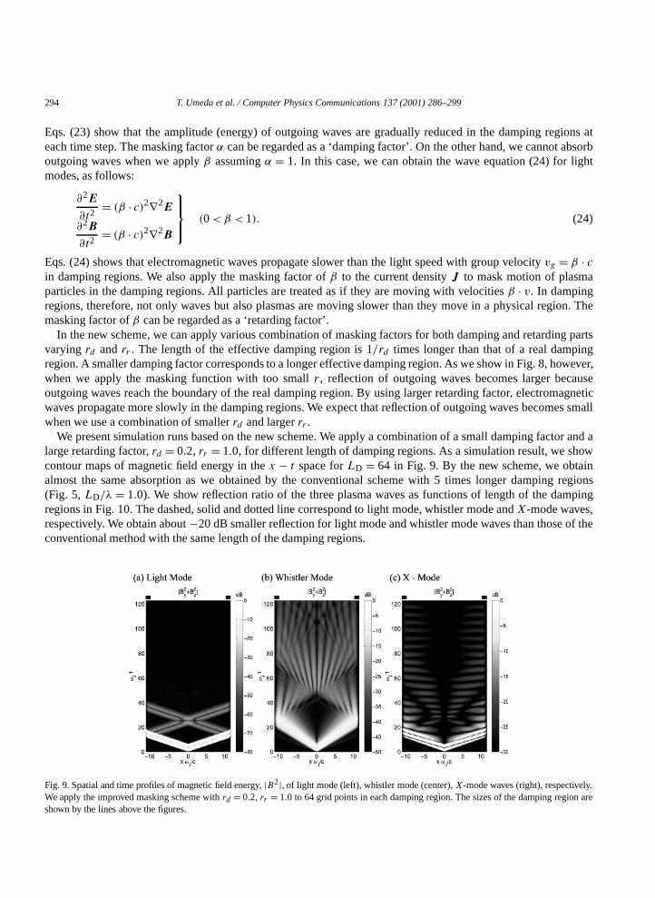
We present simulation runs based on the new scheme. We apply a combination of a small damping factor and alarge retarding factor,rd = 0.2, rr = 1.0, for different length of damping regions. As a simulation result, we showcontour maps of magnetic field energy in thex − t space forLD = 64 in Fig. 9. By the new scheme, we obtainalmost the same absorption as we obtained by the conventional scheme with 5 times longer damping regions(Fig. 5,LD/λ = 1.0). We show reflection ratio of the three plasma waves as functions of length of the dampingregions in Fig. 10. The dashed, solid and dotted line correspond to light mode, whistler mode andX-mode waves,respectively. We obtain about−20 dB smaller reflection for light mode and whistler mode waves than those of theconventional method with the same length of the damping regions.

Fig. 9. Spatial and time profiles of magnetic field energy,|B2|, of light mode (left), whistler mode (center),X-mode waves (right), respectively.We apply the improved masking scheme withrd = 0.2, rr = 1.0 to 64 grid points in each damping region. The sizes of the damping region areshown by the lines above the figures.


Fig. 10. Reflection ratio as functions of length of the damping regionLD for light mode, whistler mode andX-mode waves, respectively.λ= 314 represents wave length of light mode.

Fig. 11. Reflection ratio as functions ofrd for light mode, whistler mode andX-mode waves, respectively.LD = 64. rr = 1.0. Largerrdcorresponds to larger damping factor.

Next, we investigate the most effective combination ofrd andrr . Firstly, we varyrd with rr = 1.0 andLD = 64.The reflection ratio for differentrd is shown in Fig. 11. The best absorption for both three modes are realizedwith rd = 0.15 ∼ 0.2, i.e. the combination of smaller damping factor and larger (largest) retarding factor. Asdiscussed in Section 2, the damping factor that gives the best absorption depends on the numerical group velocityof outgoing waves. Secondly, we varyrr with rd = 0.2 andLD = 64. The reflection ratio for differentrr isshown in Fig. 12. In this case, the best absorption for both three modes are realized withrr 0.9. To see effectof retarding factor in detail, we show reflection ratio of light mode as functions ofrr for rd = 0.16, rd = 0.2and rd = 0.4, respectively, in Fig. 13. Forrd = 0.4, we have worse absorption with larger retarding factor. Asmentioned in Section 2, when we use larger damping factor (rd > r0 = 0.35), electromagnetic waves do not reachboundaries of damping regions. By using smaller retarding factor, outgoing waves propagate faster and penetratedamping regions more deeply. Forrd = 0.16 and 0.2, on the other hand, the retarding effect is important to absorboutgoing waves. Using larger retarding factor, we have better absorption of outgoing waves. However, too large


Fig. 12. Reflection ratio as functions ofrr for light mode, whistler mode andX-mode waves, respectively.LD = 64 grid,rd = 0.2. Largerrrcorresponds to larger retarding factor.

Fig. 13. Reflection ratio as functions ofrr for light mode waves withrd = 0.16, rd = 0.2 andrd = 0.4, respectively.

retarding factor gives reflection rather than absorption forrd = 0.2. For the case with a smaller damping factor(rd < 0.35), electromagnetic waves reach the boundaries of the damping regions before they are absorbed. Byusing a larger retarding factor, outgoing waves stay longer in damping regions resulting more effective absorption.As we described above, we can have better absorption with the smaller damping factor (rd = 0.16, rr = 1.0:−42.5 dB) than with the larger damping factor (rd = 0.4,rr = 0.0:−40.0 dB), because of longer effective dampingregions.

In most cases, the best retarding parameter isrr = 1.0. Because of the retarding effect, however, wave lengthof outgoing waves gradually becomes shorter(λ= 2πc/ω) and wave number of the waves becomes larger. Whenthe effective wave number becomes larger than the maximum wave number of the system (ωx/βc > kmax= π ),


Table 2Spatial damping ratio

∫ LD0 ki dx and reflection ratioΓ for parametersrd , rr ,

ND and(c tx ). ωJt = 0.015

rd rr ND c tx

∫ LD0 ki dx Γ

0.16 1.0 64 0.75 3.09 −42.5 dB

0.15 1.0 64 0.60 3.40 −43.0 dB

0.14 1.0 64 0.45 3.95 −43.2 dB

0.11 1.0 128 0.75 3.64 −54.0 dB

0.1 1.0 128 0.60 3.76 −54.7 dB

0.09 1.0 128 0.45 4.07 −55.3 dB

0.09 1.0 192 0.75 4.08 −61.8 dB

the waves cannot exist in damping regions and are reflected. We can summarize that the best retarding factor (thelargestrr ) is given by

rr =

(1− ωx

cπ

)1/2 NDND−1 for x cπ

ω

(1− (

ND−1ND

)2),

1.0 forx < cπω

(1− (

ND−1ND

)2).

(25)

It is noted that the retarding parameter must berr 1.0 because electromagnetic waves cannot propagate fasterthan the light speed. Using the same idea in Section 2, we compute effective spatial damping ratio of the newscheme, as follows:

LD∫0

ki dx =LD∫0

1− α

βctdx = LD

ct

1∫0

r2d x

2

(1− r2r x

2)dx

ND

c tx

(rd

rr

)2[ 1

2rrlog

∣∣∣∣1+ rrx

1− rrx

∣∣∣∣ − x

]ND/(ND−1)

0, (26)

where we replaceα andβ by 1− r2d x

2 and 1− r2r x

2, respectively. We investigate the best combination ofrd and

rr , and compute spatial damping ratio∫ LD

0 ki dx. We list∫ LD

0 ki dx and reflection ratioΓ for typical parametersrd ,rr , ND and(c t

x) with an effective frequencyωJt = 0.015 in Table 2. As indicated in Table 2, by setting that∫ LD

0 ki dx = 3.0∼4.0, the bestrd for light mode can be obtained.

4. Summary and conclusion

The conventional masking method can suppress reflection of various plasma waves at boundaries. Theconventional method requires substantial damping regions to absorb outgoing waves. Larger damping regions arerealized by using larger computer memory. We first introduced a new masking parameter to change the effectivelength of damping regions. Characteristics of the method with the effective damping regions are summarized asfollows:

• Assigning size of a damping regionND and effective group velocityvg tx , we can obtain the best maskingparameterr0 from Eq. (20), namely,

r0 √

10vg

tx

ND. (27)


• Effect of the masking method depends on the following values: frequency, group velocity of waves and sizeof damping regions. We need large damping regions to absorb the waves with smaller numerical frequency orwith slower numerical group velocity.

We separate the time difference form of Maxwell’s equations in two parts. The first part represents the originalelectromagnetic field values. The second part represents the increments of electromagnetic fields. We introduceanother masking factor into the increments and apply two masking factors as shown in Eqs. (21). The characteristicsof the improved masking method are summarized as follows:

• Masking the new electromagnetic field values given by sum of the original field values and increments, wecan absorb the energy of outgoing waves in damping regions. The masking factor for the new field values isregarded as a damping factor.

• By masking the increments of electromagnetic fields, electromagnetic waves propagate slowly in the dampingregions. The masking factor for the increments is regarded as a retarding factor.

• The best absorption of outgoing waves is realized with a combination of a smaller damping factor (rd < r0)and the largest retarding factor (rr ∼= 1.0).

To use the new masking method,1. Apply the damping and retarding factors to the Maxwell’s equations as shown in Eqs. (21).2. Specify the size of damping regionsND. The better absorption is given by using longer damping regions.3. Determine the retarding parameterrr from Eq. (25).4. Determine the damping parameterrd . By setting that Eq. (26) is equal to 3.0∼4.0, the bestrd can be obtained.The new scheme gives better absorption than the conventional scheme with the same length of damping regions.

Even when we use the new scheme with one-fifth of the damping regions used in the conventional scheme, we canobtain almost the same absorption. It is possible to make simulation code faster by reducing the size of dampingregions.

As we mentioned above, efficiency of the masking method depends on frequency, group velocity of waves andsize of damping regions. Characteristics on such values should be investigated in future. In the present study, weperformed simulations for only the three modes. In plasmas, there exist many electromagnetic waves which havevarious phase velocities and polarizations. Optimization of the masking method for electrostatic waves or low-frequency waves such as ion modes is left as a future study. In most cases, however, light mode waves are alwayspresent in electromagnetic particle simulations. The group velocity of light modes is the fastest, implying thatthe absorbing boundary condition is the most stringent for the light modes. Thus the characteristics of reflectionof the light modes with the new masking method listed in Table 2 are useful in most of electromagnetic particlesimulations.

It is noted that there is a similar absorbing boundary method proposed by Berenger and well known as the Per-fectly Matched Layer (PML) method [7]. In the PML method, the light modes are absorbed in a resistive layer at-tached at boundaries. Electric and magnetic conductivity in this layer are determined so that impedance is perfectlymatched with that in vacuum. In plasmas, such impedance matching conditions are not satisfied because of the fluc-tuating conduction current density formed by the thermal charged particles. Thus the complete PML is not realizedin the electromagnetic particle simulations. We also note that there is no phase retardation in the PML method, andthat the light modes propagate with the light speed in the matched layer. However, it is obvious from our resultsthat the phase retardation affects the efficiency of plasma wave absorption. Incorporation of the phase retardationeffect in the PML method may yield better absorption of plasma waves, which is also left as a future study.

Acknowledgements

We thank T. Tominaga for useful documents on the conventional masking method. We also thank H. Usui foruseful discussions. The computer simulations were performed on the KDK computer system at Radio ScienceCenter for Space and Atmosphere, Kyoto University.


References

[1] H. Matsumoto, T. Sato, Computer Simulation of Space Plasmas, Terra Sci., Tokyo, 1984.[2] C.K. Birsall, A.B. Langdon, Plasma Physics via Computer Simulation, McGraw-Hill, New York, 1985.[3] E.L. Lindman, J. Comput. Phys. 18 (1975) 66.[4] I. Orlanski, J. Comput. Phys. 21 (1976) 251.[5] T. Tajima, V.C. Lee, J. Comput. Phys. 42 (1981) 406.[6] Y. Omura, H. Matsumoto, in: H. Matsumoto, Y. Omura (Eds.), Computer Space Plasma Physics, Terra Sci., Tokyo, 1993, p. 21.[7] J.P. Berenger, J. Comput. Phys. 114 (1994) 185.