1
Analytical phase diagrams for colloids and nonadsorbing polymer
Gerard J Fleer1 and Remco Tuinier2*+
1Laboratory of Physical Chemistry and Colloid Science, Wageningen University, 6703 HB Wageningen, The Netherlands
2Forschungszentrum Jülich, Institut für Festkörperforschung, Soft Matter Group, 52425 Jülich, Germany.
*corresponding author. e-mail: [email protected] +current affiliations:
Van ‘t Hoff Laboratory for Physical and Colloid Chemistry, Department of Chemistry, Univeristy of Utrecht & DSM ChemTech Center, ACES, P.O. Box 18, 6160 MD Geleen, The Netherlands. e-mail: [email protected]

2
Abstract We review the free-volume theory (FVT) of Lekkerkerker et al [Europhys. Lett. 20 (1992) 559] for the phase behavior of colloids in the presence of nonadsorbing polymer and we extend this theory in several aspects: (i) We take the solvent into account as a separate component and show that the natural thermodynamic parameter for the polymer properties is the insertion work v, where is the osmotic pressure of the (external) polymer solution and v the volume of a colloid particle. (ii) Curvature effects are included along the lines of Aarts et al. [J. Phys.: Condens. Matt. 14 (2002) 7551] but we find accurate simple power laws which simplify the mathematical procedure considerably. (iii) We find analytical forms for the first, second, and third derivatives of the grand potential, needed for the calculation of the colloid chemical potential, the pressure, gas-liquid critical points and the critical endpoint (cep), where the (stable) critical line ends and then coincides with the triple point. This cep determines the boundary condition for a stable liquid. We first apply these modifications to the so-called colloid limit, where the size ratio qR = R/a between the radius of gyration R of the polymer and the particle radius a is small. In this limit the binodal polymer concentrations are below overlap: the depletion thickness is nearly equal to R, and can be approximated by the ideal (van ‘t Hoff) law = 0 = /N, where is the polymer volume fraction and N the number of segments per chain. The results are close to those of the original Lekkerkerker theory. However, our analysis enables very simple analytical expressions for the polymer and colloid concentrations in the critical and triple points and along the binodals as a function of qR. Also the position of the cep is found analytically. In order to make the model applicable to higher size ratio’s qR (including the so-called protein limit where qR > 1) further extensions are needed. We introduce the size ratio q = /a, where the depletion thickness is no longer of order R. In the protein limit the binodal concentrations are above overlap. In such semidilute solutions , where the De Gennes blob size (correlation length) scales as ~ with = 0.77 for good solvents and = 1 for a theta solvent. In this limit = sd ~ . We now apply the following additional modifications: (iv) = 0 + sd, where sd = A ; the prefactor A is known from renormalization group theory. This simple additivity describes the crossover for the osmotic pressure from the dilute limit to the semidilute limit excellently. (v) = 0 where R is the dilute limit for the depletion thickness . This equation describes the crossover in length scales from (dilute) to (semidilute). With these latter two modifications we obtain again a fully analytical model with simple equations for critical and triple points as a function of qR. In the protein limit the binodal polymer concentrations scale as qR and phase diagrams qR versus the colloid concentration become universal (i.e., independent of the size ratio qR). The predictions of this generalized free-volume theory (GFVT) are in excellent agreement with experiment and with computer simulations, not only for the colloid limit but also for the protein limit (and the crossover between these limits). The qR scaling is accurately reproduced by both simulations and other theoretical models. The liquid window is the region between c (critical point) and t (triple point). In terms of the ratio t/ c the liquid window extends from 1 in the cep (here t c = 0) to 2.2 in the protein limit. Hence, the liquid window is narrow: it covers at most a factor 2.2 in (external) polymer concentration.

3
TABLE OF CONTENTS 1 Introduction 1.1 General background 1.2 Phase diagrams 1.3 Contents of this paper 2 Osmotic equilibrium theory 2.1 System 2.2 Free volume 2.3 Thermodynamics 2.3.1 Separating hard-sphere and polymer contributions 2.3.2 Hard-sphere contributions 2.3.3 Polymer contribution 2.4 Binodals, critical and triple points, and critical endpoint 2.5 Chemical potential and pressure for ‘fixed q’ 3 Phase diagrams for ‘fixed q’ in terms of v 3.1 Calculation of the phase diagram 3.1.1 FS binodals 3.1.2 GL binodals 3.1.3 Triple points 3.1.4 Critical points 3.1.5 Critical endpoint 3.2 Analytical approximations 3.2.1 The exclusion limit 3.2.2 Power-law behaviour of triple and critical points 3.2.3 GL binodals and spinodals 4 Radius of gyration and overlap concentration 4.1 Radius of gyration 4.2 Overlap concentration 5 Phase diagrams for ‘fixed q’ in terms of the polymer concentration 5.1 Relation between q / a and Rq R / a 5.2 Relation between v and reduced polymer concentration y 5.3 Phase diagrams in terms of the reduced polymer concentration y 5.3.1 FS binodals 5.3.2 GL binodals 5.3.3 Critical and triple points 5.4 Phase diagrams in terms of the external polymer concentration 5.4.1 Phase diagrams at constant chain length N 5.4.2 Phase diagrams at constant particle radius a 5.5 Phase diagrams in terms of the internal concentration 5.5.1 The free volume fraction 5.5.2 Critical and triple points in internal concentrations 5.5.3 Phase diagrams at constant chain length N 5.5.4 Phase diagrams at constant particle radius a

4
6. Phase diagrams for ‘variable q’ 6.1 Concentration dependence of depletion thickness and osmotic pressure 6.1.1 Depletion thickness in flat geometry 6.1.2 Osmotic pressure 6.1.3 Protein limit 6.2 The parameters Y and q 6.3 Critical endpoint 6.4 Triple and critical curves 6.4.1 The parameters Yc and Yt 6.4.2 The parameters ( v)c and ( v)t 6.4.3 The parameters qc and qt 6.4.4 The parameters yc and yt 6.4.5 The parameters c and t 6.4.6 The parameters c and t 6.5 Phase diagrams in terms of the reduced polymer concentration y 6.5.1 FS binodals 6.5.2 GL binodals 6.5.3 Critical and triple points 6.6 Phase diagrams in terms of the external polymer concentration 6.6.1 Phase diagrams at constant chain length N 6.6.2 Phase diagrams at constant particle radius a 6.7 Phase diagrams in terms of the internal concentration 6.7.1 Critical and triple points in internal concentrations 6.7.2 Phase diagrams at constant chain length N 6.7.3 Phase diagrams at constant particle radius a 6.8 Analytical GL binodals 7. The liquid window 7.1 Summary of equations for critical and triple points 7.2 The contact potential 7.3 Analytical results for the liquid window 7.3.1 The liquid window in terms of the interaction strength 7.3.2 The liquid window in terms of the external polymer concentration 7.3.3 The liquid window in terms of the internal polymer concentration 8 Comparison with experiments and simulations 8.1 GL binodals from experiment 8.2 Critical points from experiment 8.3 GL binodals from simulations 8.4 Critical points in simulations and other theories 8.5 Free volume fraction 8.6 Tie lines 8.7 Triple points 8.8 A complete phase diagram for qR = 1 9 Concluding remarks

5
10 References

6
Glossary of conventions and symbols Units
Unless indicated otherwise, all quantities in this paper are dimensionless, with the Kuhn length as the
yardstick for all lengths, and kT for the energy. For example, the insertion work v is in units kT, and the
radius of gyration R, the depletion thickness , and the colloid radius a are all in units .
Equations In the numbered equations, often two or more (sub)equations are combined, see for example eq 2.8 or eq
2.16. When we refer to a subequation in the text, we add the letter a for the first (eq 2.16a), b for the
second (eq 2.8b), etc.
Abbreviations cep critical endpoint
cp GL critical point
tp GLS triple point
ev excluded-volume chains in a good solvent mf mean-field chains in a theta solvent
fix fixed q, i.e., and q do not depend on the polymer concentration
var variable q, i.e., and q decrease with increasing polymer concentration
Yuk Yukawa system (hard spheres with an added exponential attraction)
F, G, L, S one-phase equilibrium for a fluid, gas, liquid, or solid, respectively
FS, GS, LS, GL two-phase equilibrium (binodals) with the phases as indicated
Subscripts 0 dilute limit
1 first derivative with respect to f
2 second derivative with respect to f
3 third derivative with respect to f
value in the limit of high qR
f, g, l, s value in fluid, gas, liquid, or solid phase
p polymer
s solvent

7
fs, gs, ls, gl value along the FS, GS, LS, GL binodals
ov overlap
sd semidilute limit
Superscripts
0 hard-sphere part of thermodynamic quantities , , , pv [eqs 2.11, 2.13, 2.15]
p polymer part of thermodynamic quantities , , , pv [eqs 2.11, 2.13, 2.15]
* value at cep (e.g., q*, qR*, *, s*, *, ( v)*, etc)
~ quantity is normalized on the cep, e.g., q q/ q * , / * , / * , etc
c value at cp
t value at tp
sp value at the (GL) spinodal
Symbols (for several quantities the defining equation is given within square brackets)
a colloid radius
f /(1 ) [eq 2.4]
fcp value of f at close-packing, fcp = 2.583
ff0, fs0 value of f in coexisting F and S phases for hard spheres: ff0 = 0.970, fs0 = 1.185
g function describing the polymer contribution to [eq 2.21b, 2.30]
h function describing the polymer contribution to pv [eq 2.22b, 2.31]
h H/a = r/a 2 (ch 7)
k Boltzmann constant
k inverse relative range of attraction a (ch 7)
n N (only in ch 4)
n number of dispersed colloid particles in a volume V
np, ns number of polymer chains or solvent molecules, respectively, in a volume V
p 0/R [eq 5.1], equals 1.13 for mf and 1.07 for ev
p pressure
pv product of p and v
(pv)1, (pv)2 first or second derivative of pv with respect to f
(pv)00 value of pv in coexisting F and S phases for hard spheres: (pv)0
0 = 6.081
q size ratio /a (depends on and N) [eq 2.3b]
qR size ratio R/a (does not depend on )
q0 size ratio /a [eq 5.2]

8
qp size ratio p/a [eq 6.7]
q*, qR*, q0* value of q, qR, q0 at the cep
r centre-to-centre distance between two colloids (ch 7)
v colloid volume 4 a3/3
veff effective exclusion volume 4 a + )3/3
vs solvent (or segment) volume
vov overlap volume of two depletion layers for particles in contact [eq 7.10]
v excluded-volume parameter 1 – 2
y normalized (external) polymer concentration / ov [eq 5.6]
yi normalized internal polymer concentration / ov = y (ch 8)
A, B, C free-volume coefficients defined in eq 2.7
DX |Xt – Xc|, where X is an arbitrary quantity (sections 3.2.3 and 6.8)
F Helmholtz energy
H interparticle distance r – 2a (ch 7)
N number of segments per polymer chain, often loosely referred to as chain length
Q polynomial Af + Bf2 + Cf3 [eqs 2.5,6]
Q1, Q2, Q3 first, second, third derivative of Q with respect to f [eq 2.8]
R polymer radius of gyration
S entropy
T temperature
V volume
Vcoil coil volume 4 R3/3
W pair potential (ch 7)
Y yqR1/ [eq 6.15]
Y* value of Y in the cep
free volume fraction [eq 2.1]
* s* value of in the fluid or solid phase at the cep
e linear expansion coefficient [eq 4.1]
/(1 ) [eq 2.5]
1, 2, 3 first, second, third derivative of with respect to f [eq 2.9]
De Gennes exponent [eq 6.1]
9
depletion thickness around a sphere; range of the depletion interaction
p depletion thickness next to flat plate
0 value of p in the dilute limit
interaction strength, pair potential for particles in contact (ch 7)
1 + q [eq 2.3a], size ratio between a particle with and without depletion layer
colloid volume fraction [eq 2.12b], often loosely referred to as colloid concentration
* s* value of in the fluid or solid phase at the cep
f0, s
0 value of in coexisting F and S phases for hard spheres: f0 = 0.494, s
0 = 0.545
cp value of at close-packing, cp = 0.741
inverse range of attraction (ch 7)
colloid chemical potential
p, s chemical potential of polymer and solvent, respectively e excess chemical potential p N s
00 value of in coexisting F and S phases for hard spheres: 0
0 = 15.463
Flory exponent (R ~ N )
correlation length (blob size) in semidilute polymer solutions
external polymer volume fraction [eq 2.12c], often loosely referred to as polymer concentration
ov value of at overlap [eq 4.6]
internal polymer volume fraction [eq 2.1]
Flory-Huggins solvency parameter
reduced grand potential (v/V) [eq 2.12a]
X |X – Xc|, where X is an arbitrary quantity (sections 3.2.3 and 6.8)
osmotic pressure in the external reservoir
dilute limit of [eq 6.8]: 0 = /N
sd semidilute limit of [eq 6.9]: sd ~
v insertion work
( v)* value of v in the cep
Heaviside function (eq 3.13)
grand potential F np p [eq 2.10]

10
1. Introduction
1.1 General background
In the beginning of the previous century there was a lively debate on whether atoms exist. Various
theoretical predictions for atomic systems were made but could not yet be tested experimentally. The first
indications for the particulate nature of matter came from the field of colloids. Einstein [1] showed that dilute
colloidal particles in a solvent should obey the gas law. Von Smoluchowski [2] predicted that colloidal
particles exhibit Brownian motion, just like atoms in a gas. Perrin [3] proved that matter is particulate by
studying colloidal resin particles: he found excellent agreement with the gas law and visualized the
Brownian motion of colloidal particles. Perrin’s resin colloids followed the height-distribution according to
Boltzmann’s law in a gravity field.
An essential difference between atomic and colloidal fluids is that the pair interactions between atoms
are fixed (they are determined by quantum mechanics), whereas those between colloids can, in principle,
be adjusted [4]. A controlled way of increasing the attractive forces between colloids is by adding non-
adsorbing polymer chains. When the attraction is strong enough (i.e., above a certain polymer
concentration) phase transitions similar to those in atomic systems may then occur [5,6].
Over the last decades, the phase behavior of mixtures of colloids and nonadsorbing polymers has
gained substantial practical and fundamental interest from both experimentalists [7-9] and theoreticians
[10-16]. Nonadsorbing polymers induce a so-called depletion force between the colloidal particles, leading
to an effective attraction due to an unbalanced osmotic pressure, as first realized by Asakura and Oosawa
[17,18] half a century ago. Shortly after, Sieglaff [19] succeeded in explaining his findings for the demixing
of polystyrene chains and colloidal microgel particles in toluene on the basis of this depletion principle.
Vrij [20,21] made the first attempts to describe this phase behavior theoretically. He simplified the
polymer chains as Freely Overlapping Spheres (FOS's) which are impenetrable for the colloidal hard
spheres (HS's) but can freely overlap other FOS's. He used the resulting depletion pair interaction between
the colloids to predict the stability regions in the phase diagram of such colloid-polymer mixtures in a simple
analysis based upon the second virial coefficient. Early experiments by De Hek and Vrij [21] and Vincent et
al [22,23] confirmed the general concepts.
A few years later, Gast et al. [24] constructed a pair-wise perturbation theory for the Helmholtz energy
of a mixture of HS's plus FOS's, which enabled the computation of the colloid volume fractions in the
coexisting phases at given external FOS concentration. An osmotic equilibrium or free volume theory (FVT)
[25], in which polymer partitioning over the coexisting phases is taken into account, was later developed by
Lekkerkerker et al. [26]. This theory gives a fair description of the phase behavior of model systems of

11
colloidal dispersions of (pseudo)hard spheres mixed with well-defined synthetic polymer chains, as long as
the polymer chains are small compared to the colloids (the so-called colloid limit, where the binodal polymer
concentrations are below overlap) [27]. The theory compares well with computer simulations of HS's plus
ideal chains [10] or HS's plus FOS's [11,28,29].
In recent years, there have been significant theoretical developments which take into account the
polymeric excluded-volume interactions [30-41]. As examples of methods that enable the prediction of the
phase behaviour of colloid-polymer mixtures we mention polymer-colloid liquid state theory [31-34],
thermodynamic perturbation theories [12,35], density functional theory [36,37], a Gaussian-core model
[14,38,39], and computer simulations of HS plus self-avoiding polymer chains [40,41]. To obtain phase
lines these methods require a significant amount of numerical work.
The osmotic equilibrium theory by Lekkerkerker et al. [26] for the phase behavior of dispersions of
colloids and non-adsorbing polymer is much simpler in this respect; it serves as a standard reference
today. The starting point is the grand potential density of a system of colloids and polymer in equilibrium
with a reservoir containing only the polymer. This grand potential is separated into a HS contribution and a
polymer contribution. The HS part may be described by known expressions for the colloidal fluid and
crystalline phases. The polymer contribution is found from a build-up principle: starting from a system
without polymer, chains are added to the system until the final concentration is reached, and the polymer
contribution is calculated by integrating along this path.
The original version of the Lekkerkerker theory was formulated for ideal chains, for which the depletion
thickness is taken to be equal to the radius of gyration R of the polymer chains and for which the polymer
osmotic pressure is given by the ideal (Van ‘t Hoff) contribution /N . Here is the polymer (segment)
volume fraction in the external reservoir and N is the number of segments per chain, and is expressed in
units 3kT / , where is the Kuhn length. The parameters entering the model are the colloid volume
fraction and two ratios related to the polymer properties: the ratio Rq R / a , where a is the colloid radius,
and the ratio ovy / , where ov is the overlap concentration.
This simple model is a fair approximation for the colloid limit (R < a, qR < 1) where the polymer
concentrations at phase coexistence are below overlap (y < 1) and where the depletion thickness R is
constant; this is the appropriate polymer length scale in dilute solutions. The model breaks down in the so-
called protein limit (R > a, qR > 1) where the binodal concentrations are in the semidilute regime (y > 1) and
where the polymer length scale is the correlation length (blob size) , which is independent of chain length
and is only a (power-law) function of y. For this limit no satisfactory theory for binodal curves exists so far.

12
We shall present one in chapter 6, and we treat also the crossover between the colloid and protein limits.
Short accounts of this new theory have been published recently [42,43].
For extending the Lekkerkerker theory one has to account for several factors. The first is that, even in
the colloid limit (and even for ideal chains), the depletion thickness 0 next to a planar surface (or around a
large sphere) is somewhat larger than R. The second is due to curvature effects: the depletion thickness
around a sphere is smaller than 0. The third is to incorporate nonideal contributions to the osmotic
pressure of the polymer, which show up especially when is of order ov or above (i.e., in the protein
limit) and which make (much) larger than the ideal contribution 0 /N . Finally, also for the depletion
thickness such nonideal effects play a role: the depletion thickness next to a plate decreases with
increasing polymer concentration, from the chain-length dependent length scale 0 R in the dilute limit
( y 0 ) to the concentration-dependent length scale in semidilute solutions (y >> 1).
Aarts et al. [30] were the first to incorporate these effects into the osmotic equilibrium theory. They
used (complicated) expressions derived from renormalization group (RG) theory [44] for the dependences
0/ and / 0 on the ratio ovy / , and also accounted for 0 /R 1 and for curvature effects. They
presented a few examples of phase diagrams for polymer chains in the excluded-volume limit and
calculated (numerically) gas-liquid critical points and gas-liquid-solid triple points. An important result of their
work is that even in this more sophisticated model the same three parameters , Rq R / a , and ovy /
are sufficient to describe the phase behavior. The authors did not address the conversion from the
normalized parameters Rq and y towards polymer chain length and polymer concentration. For this
conversion information about the dependence of R and ov on chain length and solvency is needed.
Moreover, their thermodynamic treatment (like that in the original Lekkerkerker theory) is incomplete in so
far that the solvent is treated as background, and not taken into account as a separate component. In
addition, their correlation length in semidilute polymer solutions is too small [44].
In this paper we review the thermodynamic basis of the osmotic equilibrium theory and we extend this
theory in several aspects. The most important feature is that we shall deal with the crossover in length
scales, from coil size R to blob size , which extends the validity of the osmotic equilibrium theory towards
the protein limit. Another aspect is that we explicitly account for the solvent component. The solvent
chemical potential is directly related to the osmotic pressure of the polymer solution. We show that the
product v, where 3v (4 / 3)a is the colloid volume, is the natural parameter for describing the
thermodynamics. The thermodynamic parameters are then the colloid concentration , the effective size
ratio q a, and the product v, which is the osmotic work of inserting a colloid particle (without depletion

13
layer) into the polymer solution. We will show that q and v can be simply expressed in the ratios
ovy / and qR = R/a.
1.2 Phase diagrams
In figs 1.1 and 1.2 we illustrate the basic features of v phase diagrams for the colloid limit; at this
stage we still assume that the depletion thickness (and, hence, q = /a) does not depend on polymer
concentration. We will see later that in the general case where depends on the polymer concentration the
qualitative features are the same (and the quantitative differences in a v representation are small).
Figure 1.1 shows an example of a GL binodal (dashed), a GS binodal (dotted) and an FS binodal
(solid); in this example q = 0.4. The GL binodal is only stable in a relatively small v window, in between
the lowest value c( v) corresponding to the GL critical point (cp, indicated by the diamond) and the
highest value t( v) corresponding to the triple point (tp, the three open circles connected by the horizontal
dotted line). Above the triple point there is GS equilibrium between a (very) dilute gas phase and a
concentrated solid phase. The FS binodal is stable for tv ( v) and the coexistence concentrations are
close to the well-known HS coexistence concentrations 0.49 (liquid) and 0.54 (solid); the pressure p
at this HS coexistence (see section 2.3.2) corresponds to pv = 6.08 (kT units).
Figure 1.1 applies to one particular size ratio q a 0.4. Figure 1.2 demonstrates how the
coordinates of the critical point (cp) and the triple point (tp) vary with q. The diamond (cp) and circles
(tp) are the same as in fig 1.1 (q = 0.4). As q decreases (in the direction of the arrows), c( v) and c
increase, as shown by the critical curve (label cp) in fig 1.2. This figure also shows the triple curve
(label tp) which, obviously, has three branches for the three coexisting phases. Each triple point at
given q is characterized by four coordinates: t( v) and three compositions tg , t
l , and ts . For high q
(above 0.6), where the polymer is essentially absent from the condensed phases, t( v) equals 6.08
(dashed line in fig 1.2), which is the value of pv in a HS system without polymer; t( v) cannot drop
below this value.
With decreasing q, the fluid compositions tg and t
l of the triple point approach each other; the
liquid window narrows. At a critical value q* (about 1/3) the values of tg and t
l merge at the critical
value , which marks the endpoint of the stable part of the critical curve (left asterisk in fig 1.2). At
that point there is equilibrium with a solid phase of composition s (right asterisk). The two asterisks in
fig 1.2 correspond to the critical endpoint (cep), which is a central feature in the phase diagram

14
because it constitutes the boundary condition for the existence of a stable liquid phase. This cep is
again characterized by four coordinates: q*, ( v) , *, and s .
1.3 Contents of this paper
In chapter 2 we (re)formulate the thermodynamic background of the osmotic equilibrium theory in
terms of the parameters , q a, and v. The treatment is general in the sense that and q may
depend on the polymer concentration, and and may contain nonideal contributions. We present
analytical expressions for the colloid chemical potential and the product pv, where p is the pressure
of the system; both and pv have a hard-sphere part and a polymer contribution (defined in terms of
v). We find also analytical expressions for the first and second derivatives of pv with respect to ;
these derivatives are needed for calculating GL critical points. We then show how in the general
case binodals are found from solving two equations in two unknowns (the coexisting compositions).
Also the calculation of GL critical points requires solving two equations in two unknowns (in this case c( v) and c ). For the triple points we have to solve four equations in four unknowns: t( v) and
three coexisting compositions. Finally, also the critical endpoint follows from four equations in the four
unknowns q*, ( v) , *, and s .
For the special case of a constant polymer length scale (hence, and q are independent of the
polymer concentration or v), the equations may be simplified. We denote this situation as ‘fixed q’.
Now the calculation of all the characteristic points (binodal points, critical points, triple point, critical
endpoint) may be reduced to solving one equation in one unknown and a fully analytical phase
diagram can be obtained. This situation is discussed in chapter 3. It is found that the cep is situated at
q* 0.328, ( v) 10.73 , * 0.319, and s 0.593 . We show that the essential features of the
phase diagram (critical curve, triple curve) may be approximated quite well through power laws in the
reduced quantities / * , v v /( v) * , and q q/ q * , obtained by normalizing on the cep.
This again illustrates the central role of the cep in phase diagrams. Throughout this paper we use *
(asterisk) to denote the cep and ˜ (tilde) to indicate that the quantity of interest is normalized on the
cep.
The parameter q may be simply related to the size ratio Rq R / a ; for ‘fixed q’ the approximate
relation is 0.9Rq 0.9q , which accounts for curvature effects. The parameter v can be expressed in
ovy / and Rq in a very simple way: 3Rv q y in dilute solutions. Hence, v( ) diagrams for
various q may be converted to y( ) diagrams for various Rq . This conversion is discussed in chapter

15
5. In order to convert the normalized parameter y to the real concentration for a given polymer chain
length N and solvency v (where is the Flory-Huggins parameter) one has to know how the
overlap concentration ov and the radius of gyration R depend on N and v. Preceding the discussion
of y( ) phase diagrams in chapter 5, we address this issue in chapter 4. We present explicit
expressions for ov (N,v) and R(N,v) for mean-field (mf) chains in a theta solvent (v = 0) and for
excluded-volume (ev) chains in a good solvent (v > 0), and we give useful approximate scaling
relations (including the numerical prefactors) for these dependencies. Whenever we use the
abbreviation mf we refer to a theta solvent, while ev refers to a good solvent.
As stated above, chapter 5 gives y( ) and ( ) phase diagrams for ‘fixed q’. The cep turns out to
be situated around y* = 0.35, which is indeed well below overlap (y = 1): for the region around the cep
the approximation of a constant q is thus reasonable. For the phase diagrams we distinguish
between two cases. The first is constant R, so q is varied by adjusting the particle radius a. In this
case ov does not depend on q, and is constant across the entire phase diagram; then / * y/y* or
y . The second situation is that of constant particle radius a, whereby q is varied by changing R.
Now ov is a function of q and the relation between and y is slightly more complicated. To a good
approximation it is 1Ryq (mf) or 4/ 3
Ryq (ev). For both situations (constant R and constant a) we
give simple analytical expressions (qR) for critical and triple points.
In the final section of chapter 5 we also discuss ( ) phase diagrams in terms of the internal
concentrations , where is the fraction of free volume in each phase. This fraction depends
strongly on the colloid concentration. One of the implications is that, whereas in terms of v or the
external concentration the triple point may be represented as a horizontal line (see fig 1.1), the
internal concentration t differs strongly in the three coexisting phases, and the horizontal triple line is
converted into a triple triangle.
Chapter 6 constitutes the most important part of this paper. We introduce a concentration-
dependent polymer length scale, which enables the calculation of phase diagrams for any polymer
concentration, including the protein limit. The depletion thickness decreases from R in dilute
solutions towards it semidilute limit = ~ , where is the correlation length (blob size) and is the
De Gennes exponent which equals 1 in a theta solvent (mf) and ¾ (or 0.77) in good solvents (ev).
Simultaneously, the osmotic pressure displays a crossover from the dilute limit = 0 = /N
towards the semidilute limit = sd ~ 3 ~ . This situation is denoted as ‘variable q’.

16
We employ very simple – yet accurate – expressions proposed recently [45,46]: 2 20 1( / ) 1 c y
and 3 10 2/ 1 c y , where c1 and c2 are known constants of order unity. Clearly, in semidilute
solutions these expressions reduce to sd ~ and sd ~ , but they apply also to the dilute limit ( =
0, = 0) and describe the crossover region as well. The relation 3Rv q y for the dilute case is now
extended to 3 3Rv q (y b y ) , where b is a known constant. Hence, the general equations given in
chapter 2 may be formulated either in terms of v or in terms of y; for mathematical reasons the
variable y is now easier to implement.
This generalized ‘variable q’ model describes both the colloid limit and the protein limit, as well as
the crossover. It gives about the same cep as the ‘fixed q’ model based upon 0 and 0 ,
which is not surprising because we concluded in chapter 5 that the cep is located within the dilute
regime (y* 0.35). Perhaps more surprising is the fact that outside the cep, even when y is well above
unity, v( ) phase diagrams are qualitatively (and nearly quantitatively) the same as in the dilute
situation (although the range for Rq is very different). This again shows the relevance of the
parameter v in the thermodynamics. This equality does not hold for ( ) phase diagrams, because
the dependence v(y) at finite concentrations is very different from that in dilute solutions. However,
also for concentrated polymer solutions and in the protein limit simple analytical equations (e.g., for
critical and triple points) describe the phase diagrams quite well, with power-law exponents which are
different from those in the colloid limit. In the protein limit we find a surprisingly simple result: the
binodal concentrations scale as qR and normalized phase diagrams yqR versus become
independent of the size ratio qR = R/a.
In chapter 7 we discuss the liquid window, which is the parameter range over which a colloidal
liquid is stable. In terms of the (external) polymer concentration it may be defined as the region yc < y
< yt, where the superscripts refer to critical and triple points, respectively. The reference point is the
cep, where qR* 1/3 and yc = yt = y* 0.35; in the cep the width of the liquid window is zero. With
increasing qR the window yt yc widens. In the ‘fixed q’ model yt yc increases with qR without bounds,
but this model loses its validity for high qR. For the new ‘variable q’ model the behavior close to the
cep (i.e., in the colloid limit) is nearly the same, but for high qR (protein limit) the ratio yt/yc becomes
constant: yt/yc 2.2. Then for given qR the liquid window spans only a factor 2.2 in the external
polymer concentration . In terms of the internal polymer concentrations this ratio is somewhat
larger (about 3 for the gas branch and an additional factor 2.5 for the liquid branch of the binodal), but
anyhow there is only a limited range of polymer concentrations over which a colloidal liquid is stable.

17
The liquid window may also be expressed in terms of the interaction strength , which is the value
of the pair potential for two colloidal particles in contact. Clearly, t c is zero in the cep, and t c
increases with qR for qR > qR*. It turns out that for ‘fixed q’ this increase is again without bounds,
whereas for ‘variable q’ a maximum level of about 1.6 kT is attained. There is thus only a limited range
of interaction strengths over which a liquid is stable. This balance is even more subtle for a one-
component Yukawa fluid, where the liquid window t c is no more than (at most) 0.6 kT.
In the final chapter 8 we compare our ‘variable q’ theory with experiments, with simulations, and
with other theories, for both good and theta solvents. In most cases we find semiquantitative
agreement with experimental critical points and GL binodals. Also the agreement with simulations is
quite good. Other theories sometimes deviate considerably from our prediction in the quantitative
aspects, but the qualitative behavior is usually the same. A very important feature is that our qR
scaling law is accurately reproduced by both simulations and other theories which are applicable to
this limit.

18
2. Osmotic equilibrium theory 2.1 System
We consider a system where two phases with different colloid and polymer concentrations are in
equilibrium with each other and with an external reservoir containing only the polymer solution (see fig 2.1).
The phase concentrated in colloid may be solid (S) or liquid (L), the dilute phase may be gas-like (G) or
liquid. We also use the term fluid (F) to denote either the G or the L phase; beyond the critical point there is
no difference between G and L. In some cases S may be in equilibrium with two F phases (one liquid and
the other gas); we then have a triple point where three phases coexist.
The chemical potential of the polymer in the system is determined by its volume fraction in the
reservoir. This volume fraction is unity in the polymer melt. In the colloid phases, the local polymer
concentration in the free volume not occupied by the particles (plus the depletion layers surrounding them)
is the same as the external concentration . However, the overall internal concentration is lower because
the free volume is smaller than the total volume:
x x [2.1]
where x G, L, or S and the exclusion factor is the fraction of the volume available for the polymer.
When the system is dilute in colloids, the depletion layers around the particles do not overlap and
one expects a simple form for : eff(V nv ) / V , where V is the volume of the system, n the
number of dispersed colloids in it, and eff 3v (4 / 3)(a ) the effective volume excluded for the
polymer chains by one colloid particle; here a is the bare particle radius and is the thickness of the
depletion layer around the sphere. The depletion layer is indicated by the grey halo around the
particles in fig 2.1.
We define the dispersed colloid volume fraction as nv / V , where 3v (4 / 3)a is the bare
colloid volume. For low the free volume fraction equals 31 (1 / a) or
31 (small or q) [2.2]
where the parameter is the size ratio between particles with and without a depletion layer:
1 q qa
[2.3]
The parameter q is the ratio between the depletion thickness (which is the range of the attraction) and the
particle radius; it may be seen as the relative range of the attraction. The quantity 3 effv / v is the
normalized volume (per particle) which is inaccessible for the polymer chains in a dilute colloid phase.
We note that is the depletion thickness around a colloidal sphere, which in dilute polymer solutions
and for relatively large particles is of order of (but not equal to) the radius of gyration R of the polymer coils.

19
In general, the parameter q a is not equal to Rq R / a . In section 5.1 we show that in the colloid limit
(where is independent of the polymer concentration) the two parameters are related through 0.9Rq 0.9q
(for a more precise result see eq 5.5). In more concentrated solutions, where decreases with increasing
, the relation between q and Rq becomes -dependent, see section 6.2 (eq 6.17). We will see that in the
protein limit (qR > 1) q becomes independent of qR. In most of the present chapter 2 and in chapter 3 we
use only the parameter q (or 1 + q), without specifying the relation with Rq .
For more concentrated colloid phases the depletion layers do overlap and the fraction of the volume
which is excluded for the polymer is less than 3 due to (multiple) overlap of depletion layers; is then
higher than according to the limiting form of eq 2.2. A more general expression for is given by scaled-
particle theory for the free volume [26,47], to be discussed in the next section. This theory is based upon
the particle insertion method by Widom [48]. The free volume fraction follows from the work required to
insert a polymer chain into a sea of colloidal spheres.
2.2 Free volume
In scaled-particle theory the free volume fraction depends solely on the parameters (colloid
volume fraction) and q or (effective size ratio), regardless of the type of phase (G, L or S). The
expressions are more transparent when the ratio /(1 ) is used as the variable rather than itself.
Therefore we define a concentration parameter f :
f1
f1 f
[2.4]
The scaled-particle expression [26] for may be written as (1 ) Qe [2.5]
where Q is a polynomial in f: 2 3Q A f Bf Cf [2.6]
The coefficients A, B, and C are a function of q only:
3A 1 2B 3q q 3 / 2 3C 3q [2.7]
For small f and not too large q, 1 Af and 1 (A 1)f , so eq 2.2 is recovered. For large f and
finite q, and approach zero, as expected for concentrated colloid systems (see the concentrated
phase in fig 2.1). It has been shown that the prediction of eq 2.5 for the free volume fraction agrees
very well with computer simulation results [10,29], at least when q is O(1) or below.
A plot of for five values of q is given in fig 2.2. The initial part for small is linear according
to 31 (eq 2.2); this linear part extrapolates to 0 at 3 . For the three lowest q values in

20
fig 2.2 this limiting form is shown as the dashed lines; for low q this form describes over a wide
concentration range. For high q, decays to zero at relatively small : the polymer is then largely
excluded from the colloid phase. This effect is very pronounced for q 5: the exclusion is then
essentially complete for any , even in very dilute systems. In this high-q limit Q Af and Afe .
Hence, the exclusion limit applies when f exceeds the value 31/ A by, say, a factor of 3.
We note that in the ‘fixed q’ model (where q is of order qR) q is an independent variable which
may be assigned a high value. However, for ‘variable q’ (to be discussed in chapter 6) q depends not
only on qR but also on the polymer concentration. In that case q remains below unity, even when qR is
high (protein limit).
We will also need derivatives of and, hence, of Q and with respect to f. When we abbreviate n nX / f as nX , we may write
21
2
3
Q A 2Bf 3CfQ 2B 6CfQ 6C
[2.8]
1 1
2 2 1 1
3 3 1 2 2 1
QQ QQ 2 Q Q
[2.9]
These expressions are needed to find, for given q, the chemical potential, the pressure, the critical point,
and the critical endpoint.
2.3 Thermodynamics
2.3.1 Separating hard-sphere and polymer contributions
For a system with given numbers n of colloids and pn of polymer chains in a given volume V at
temperature T the characteristic thermodynamic function is the Helmholtz energy pF(T,V,n,n ) , with
total differential p pdF SdT pdV dn dn , where and p are the chemical potentials of the
colloid particles and of the polymer, respectively. For the moment we disregard the solvent, as in the
original theory, but we shall correct for this in section 2.3.3. For a semi-open system like in fig 2.1 the
variable pn has to be replaced by the variable p . The corresponding characteristic function is the
grand potential p(T,V,n, ) , obtained by a standard Legendre transformation as
p p p p(T,V,n, ) F(T,V,n,n ) n [2.10]
Its exact differential is p pd SdT pdV dn n d , showing that the variable pn in F is replaced
by the variable p in . The colloid chemical potential is found by differentiating with respect to

21
n. Integrating the exact differential gives pV n . Hence, when is known and p are readily
obtained.
Following Lekkerkerker et al. [26] and Aarts et al. [30] we write 0 p , where 0 0F is the
Helmholtz energy of a hard-sphere system without polymer and p is the polymer contribution. The
latter is found from a build-up principle: starting from a system without polymer ( 0 , p ),
polymer is added to the system until the final concentration is reached. Hence,
0 p p
pp pn d [2.11]
Since 0d SdT pdV dn and pp pd n d , in eq 2.11 has the same exact differential as
in eq 2.10. The assumption made in eq 2.11 is that the polymer does not affect the configuration of
the colloids.
The polymer contribution p is evaluated using the free volume theory outlined in section 2.2,
whereby the polymer concentration in the colloid phases is lower than in the reservoir by a factor
which depends on f and q. It is convenient to rewrite eq 2.11 in terms of reduced quantities:
vV
v nV
sp
Nv nV
[2.12]
where v is the colloid volume, sv the segment (or solvent) volume, and N the number of segments
per polymer chain; the volume occupied by the segments of a chain is sNv . Now eq 2.11 transforms
into
0 p p
pp
s
v dNv
[2.13]
where in the polymer term we applied eq 2.1.
The chemical potential of the colloids and the pressure p in the system are found from the standard
thermodynamic relations pT,V,( / n) and pV n :
pv [2.14]
Clearly, these quantities have a hard-sphere part and a polymer contribution: 0 p 0 ppv (pv) (pv) [2.15] We discuss these contributions separately in the next two sections.

22
2.3.2 Hard-sphere contributions
For a dispersion of hard spheres we have 0 . For a fluid phase a very accurate expression is due
to Carnahan-Starling [49], and for a crystalline solid phase we use an expression based on work by Hall
[50] with a numerical constant that follows from computer simulation results [51]:
2
0
1 1cp
ln 1 4f f fluid
2.1306 3ln solid [2.16]
where cp ( / 6) 2 0.741 is the volume fraction at close-packing. Applying eq 2.14 (with 2df (1 f ) d ) gives the following equations for the chemical potential and the pressure:
2 3
01 1 1 1
cp cp
ln 8f 7f 2f fluid2.1306 3 /( ) 3ln( ) solid
[2.17]
2 3
01 1 1 1
cp cp
4f 2f fluid(pv)
3 ( ) 3 (f f ) solid/ / [2.18]
where cp cp cpf /(1 ) 2.853 . Both 0s and 0
s(pv) for a solid diverge at close-packing:
cp 0.741 or cpf f 2.853 .
For calculating GL critical points and the critical endpoint we will also need the first and second
derivatives of eq 2.18a with respect to f:
0 2 210 32
(pv) (1 f) 8f 6f
(pv) 2(1 f) 8 12f [2.19]
Note that a numerical subscript 1 or 2 denotes the first or second derivative with repect to f.
Figure 2.3 gives plots of 0f and 0
s (dashed curves) and of 0f(pv) and 0
s(pv) (solid) as a function
of f . There is a well-known fluid-solid phase coexistence at 0f 0.494 and 0
s 0.545 according to
computer simulations [52-54]. Essentially the same result follows from the above equations with the
condition 0f 0
s and 0fp 0
sp : 0ff 0.970 ( 0
f 0.492 ) and 0sf 1.185 ( 0
s 0.542 ). This coexistence
condition is indicated by the rectangle in fig 2.3, with 00 15.463 and 0
0(pv) 6.081 at coexistence.
These numbers may be calculated by writing 0s cp1/ f 1/ f 3 / (pv) from eq 2.18b. Substituting
0 0f fp p (f ) from eq 2.18a gives sf as a function of ff . Inserting this relation into 0
f f(f ) 0s s(f ) leads to
an implicit equation in ff which is easily solved numerically. This procedure is entirely equivalent to
applying the common tangent construction to 0f (f) and 0
s(f) .
2.3.3 Polymer contribution
We rewrite the polymer contribution of eq 2.13b in terms of the osmotic pressure of the external
reservoir, taking the solvent into account as a component. When the solvent is treated as

23
background, the solvent molecules do not occupy volume, and polymer chains can be added to the
system without affecting the solvent. We treat the solvent molecules as entities occupying the same
volume sv as polymer segments. The implication is that upon adding one polymer chain to the system
N solvent molecules have to leave. Consequently, we replace p in eq 2.13b by an exchange
chemical potential e , defined by ep sN , where s is the chemical potential of the solvent.
In eq 2.13b we then need ep sd d Nd . From the Gibbs-Duhem rule we have p pn d
s sn d 0 , where sn is the number of solvent molecules. In terms of this gives pd
s1 Nd esd Nd 0 . Since s sv , we obtain e
sd Nv d , so eq 2.13b can be
written in the simple form
v
p
0
d v [2.20]
We see that the product v is a natural parameter in the thermodynamic description. It is the osmotic work
to insert a particle (without depletion layer) into the polymer solution. Equation 2.20 is general, but for
applying it the relation between and v is needed. We recall that is a function of f and q a. In the
colloid limit, where is constant (independent of or ), eq 2.20 simplifies to p v (see also eq
2.29). In the general case where and q decrease with increasing v, the integration of eq 2.20 cannot be
avoided; one then has to specify the relation between q and v.
Applying again eq 2.14 we obtain the polymer contributions to and pv:
v
p 3
0
gd v 31g (1 f) [2.21]
v
p
0
(pv) hd v 1h f [2.22]
The functions g and h are defined in terms of (eq 2.5) and its first derivative (eq 2.9). For f = 0, = 1
and 1 = A, so h = 1 and 3g = 1 + A = 3 or g = 1. For large f, = 1 = 0 and g = h = 0. Plots of the
functions g and h as a function of f are given in fig 2.4. Both functions decay in roughly the same
way from unity in dilute systems to zero in concentrated colloidal dispersions. This decay is faster as q
increases. The function g (solid curves) for intermediate f is somewhat smaller than the function h
(dashed). For large q (see the curve for q 5 in fig 2.4) g and h reach the limits Afg e and Afh (1 Af)e so g and h are essentially zero for 1f A or 3f . Then we have the exclusion limit
0 and 0p p for nearly any colloid concentration.
For the calculation of critical points we need the first and second derivatives of eq 2.22 with respect to
f. These derivatives may be written in terms of the second and third derivatives of (defined in eq 2.9):
24
vp1 2
0v
p2 2 3
0
(pv) f d v
(pv) ( f )d v [2.23]
2.4 Binodals, critical and triple points, and critical endpoint
Binodal points are obtained from equal chemical potentials (eqs 2.17 plus 2.21) and equal pressures
(eqs 2.18 plus 2.22) in the two coexisting phases:
FS f s f s(pv) (pv) [2.24]
GL g l g l(pv) (pv) [2.25]
Here g f(fg) and l f(fl), and similarly for pv.
For the GL critical points the first and second derivatives of the pressure (or the chemical
potential) with respect to f are zero:
cp 1 2(pv) (pv) 0 [2.26]
The two contributions to these derivatives are given in eqs 2.19 and 2.23, respectively.
Triple points follow from equal chemical potentials and pressures in three phases:
tp g l s g l s(pv) (pv) (pv) [2.27]
Finally, for the cep we have critical conditions supplemented with equal chemical potential and
pressure in fluid and solid phases:
cep 1 2(pv) (pv) 0 f s f s(pv) (pv) [2.28]
In order to apply these expressions, we have to specify how q in the integrals of the polymer
contributions depends on Rq and v. We postpone the general formulation of this problem to chapter
6, but we give one example of the type of dependence. It can be shown that in a semidilute good
solvent 3 2.31Rv ~ q y (eq 6.12) and 0.88 0.68
Rq ~ q y (eq 6.17), where ovy / . Combining these two
relations we find 0.37q ~ ( v) , independent of R or Rq , as expected for semidilute solutions. Inserting
these relations (with the appropriate numerical constants) into the integrals for p and p(pv) , we could
from eq 2.24 or 2.25 solve the two equations in the two unknown compositions ( ff and sf for FS, gf
and lf for GL) at given Rq and v to find the binodals. Similarly, we could from eq. 2.26 (again two
equations in two unknowns) find v and f at given Rq to obtain the critical points.
For finding triple points, we have to solve the four equations of eq 2.27 for v and three
compositions, again at given Rq . Finally, the cep follows from solving the four equations of eq 2.28 for
Rq , ( v)*, f*, and sf .

25
The procedure outlined above is inaccurate since the scaling relation 0.37q ~ ( v) breaks down in
the dilute regime (y < 1). It is possible (see section 6.2) to find relations Rv(q ,y) and Rq(q ,y) which
are valid over the entire concentration range. However, now the relation Rq(q , v) is implicit, which is
computationally unhandy. It is then easier to use y instead of v as the integration variable, replacing
d v in the integrals by ( v / y)dy . Details of the necessary expressions are given in section 6.2. 2.5 Chemical potential and pressure for ‘fixed q’
When q does not depend on v, which is the case in the colloid limit, the integrand in eqs 2.20-22 is a
constant and may be taken out of the integral. Now , , and pv reduce to
0 v [2.29]
0 3v g [2.30]
0pv (pv) vh [2.31]
Similarly, eq 2.23 may be simplified and the first and second derivatives of pv are given by
0
1 1 20
2 2 2 3
(pv) (pv) f v
(pv) (pv) ( f ) v [2.32]
Now all eqs 2.24-28 for calculating binodals, critical and triple points, and the cep can be rewritten
such as to give one equation in one unknown. For example, eq 2.24 for FS binodals reduces to 0 3 0 3f f s sv g v g and 0 0
f f s s(pv) vh (pv) vh , from which v may be eliminated. The
result (which is shown in eq 3.1) gives a direct relation between ff and sf . So when a value for sf is
chosen, ff follows immediately from solving one equation in one unknown.
In the next chapter we calculate full phase diagrams for ‘fixed q’. First we illustrate some features
of the simple equations 2.30-31 for and pv. An example of (f) and pv(f) for a fluid phase ( 0 0f ,
0 0f(pv) (pv) ) is given in fig 2.5, for q 0.6 ( 1.6 ) and three values of : 1v 2 , 2v 2.259
and 3v 2.738 . The value of 2 corresponds to c , the osmotic pressure at the critical point.
For a low polymer concentration (say, 1 ), both and pv increase monotonically with the
colloid concentration. Hence, there is no possibility for phase separation into a dilute G phase and a
concentrated L phase, since such a demixing requires equal and p in both phases. For a high
polymer concentration ( 3 ), both and p show a Van der Waals loop. In this particular example
we have equal ’s ( 7.878 ) at three points: gf 0.052 , lf 0.5 and a metastable point somewhere
in between. For this we have equal p ’s (pv 2.779 ) at exactly the same colloid concentrations, so
these two points gf 0.052 and lf 0.5 lie on the binodal.

26
In between, for c , there is an inflection point with zero slope in both curves at cf f . In this
point the first and second derivatives of and p are zero. From these conditions, the location of the
critical point, which is the lowest point of the binodal, may be derived, see eq 2.26; for q = 0.6 the
result is ( v)c = 2.259 and fc = 0.231.

27
3 Phase diagrams for ‘fixed q’ in terms of v
In this chapter we assume that and q are independent of the polymer concentration (so eqs 2.29-32
apply) and we use only the product v to characterize the polymer solution. There is no need to
specify how depends on the polymer concentration . The conversion towards is discussed in
chapter 5.
3.1 Calculation of the phase diagram
3.1.1 FS binodals
Substituting eqs 2.30-31 into eq 2.24 gives 0 3 0 3f f s sv g v g for the chemical potentials
and 0 0f f s s(pv) vh (pv) vh for the pressures. After eliminating v from these two relations, we
obtain:
0 0 0 0s f s f
3f s f s
(pv) (pv)1vg g h h
[3.1]
Here 0f (eq 2.17a) and 0
f(pv) (eq 2.18a) depend only on ff , and 0s (eq 2.17b) and 0
s(pv) (eq 2.18b)
only on sf . For a given value of q, the same applies to the g ’s and h ’s, respectively. Hence, the
second and third parts of eq 3.1 give a unique relation ff ( sf ): when a value for sf is chosen, the
corresponding value of ff is found by solving the second equality of eq 3.1, and v follows
immediately from the first. Figure 3.1 gives six FS binodals, for q 0.2, 0.26, 0.3275, 0.35, 0.4, and
0.6. The value q* 0.3275 corresponds to the critical endpoint, see eq 3.7 which gives the precise
coordinates of the cep.
All F branches in fig 3.1 start at 0ff 0.970 and all S branches at 0
sf 1.185 for v 0; these are
the hard-sphere coexistence concentrations discussed in section 2.3.2, see fig 2.3. For thin depletion
layers (q 0.2), there is not much difference with hard spheres without polymer. Also the pressure of
the system does not deviate much from that of hard spheres (pv 6.08) because h in eq 2.31 is
small. The composition of the fluid phase becomes slightly more dilute and that of the solid phase
more concentrated as v increases: the miscibility gap widens somewhat as the polymer
concentration goes up. For slightly thicker depletion layers (q 0.26) this widening is more
pronounced at high v .
For q q* 0.3275, the F-branch is nearly horizontal over a wide range of colloid concentrations
and it has an inflection point with zero slope of the curve. This inflection point (top circle left) is the
fluid part of the cep, situated at v 10.73 and f 0.467 (see eq 3.7). The solid branch has a
discontinuity in slope at the same v and f 1.457 (top circle right), which is the solid part of the cep.

28
When q > q*, the fluid branch becomes discontinuous (there is a jump from the L branch to the G
branch at a certain v), and the discontinuity in slope of the solid branch (at the same v) becomes
more pronounced. For example, for q 0.35 this discontinuity occurs at v 9.66 and f-values 0.193
(G), 0.724 (L), and 1.398 (S). This is the triple point for this q value, where three phases coexist. For q
0.4 the triple point coordinates are v 8.05 and f 0.054 (G), 0.857 (L), and 1.306 (S), and for q
0.6 these values are v 6.18 and f 7.10 (G), 0.962 (L), and 1.193 (S). The coordinates of these
three triple points are also indicated as closed circles in fig 3.1.
For still higher q the FS binodals and the triple point coordinates are nearly the same as for q
0.6. This is because for very thick depletion layers the polymer is nearly fully excluded from the
condensed phases. Hence, in eq 2.31 the polymer contribution may be neglected (h 0), so 0spv (pv) in the solid phase. In the (very) dilute gas phase the polymer contribution dominates:
pv v since h 1 and the colloid contribution to the pressure is negligible. Since the two coexisting
phases should have the same pressure 0sv (pv) , with 0
s(pv) the hard-sphere contribution given by
eq 2.18b. The binodal for q is indicated by the crosses in fig 3.1. The gas branch coincides with
the ordinate axis, the solid branch follows 0sv (pv) , which is the part f > fs
0 of 0s(pv) in fig 2.3. The
triple-point value of v in this limit is where the solid branch intersects the vertical line at 0sf f 1.185 , and is given by 0
0(pv) 6.081.
3.1.2 GL binodals
Analogously to eq 3.1 the coexistence concentrations gf and lf follow from the relations 0 3 0 3g g l lv g v g and 0 0
g g l l(pv) vh (pv) vh , or
0 0 0 0l g l g
3g l g l
(pv) (pv)1vg g h h
[3.2]
where 0 0l f l(f ) and 0 0
g f g(f ) , with 0f given by eq 2.17a, and similarly for the 0(pv) ’s and eq
2.18a. In eq 3.2 the same functional form for 0f and 0
f(pv) for the coexisting phases applies, whereas
in eq 3.1 these forms are different.
Figure 3.2 gives some examples of GL binodals, for q 0.3275 ( q*), 0.35, 0.4, and 0.6. The GL
binodal for q q* is a single point (point binodal), and for higher q the binodal spans a wider region,
both in terms of the colloid concentration range and in terms of v. The endpoints left and right of
each binodal are the G and L parts of the triple point (circles; these are the same as in fig 3.1), the
minimum is the critical point (diamonds); it follows from eq 2.26 in combination with eq 2.32. The
coordinates of the three critical points are v 9.02, f 0.434 for q 0.35, v 6.38, f 0.374 for q

29
0.4, and v 2.26, f 0.231 for q 0.6. For comparison, the two binodal points for q 0.6 from fig
2.5 are indicated as the two squares in fig 3.2.
The plusses in fig 3.2 give the high-q limit for the GL binodal, obtained in the same way as the
crosses in fig 3.1 by assuming exclusion of the polymer from the liquid phase. Hence, the G branch
coincides with the ordinate axis, and the L branch is 0fv (pv) , given by eq 2.18a. In this limit the
critical point is at v f 0. This is a typical ‘fixed q’ result; we will see later that when q is allowed to
vary with polymer concentration a nonzero value is found for high qR = R/a.
3.1.3 Triple points
In a triple point we have equal p ’s and ’s at three compositions. We may write down three
equations of the type of eq 3.1 or 3.2, for the GS, GL, and LS coexistence, respectively. Obviously,
we need only two of those. When we choose GL and LS we have
0 0 0 0l g l g
gl 3g l g l
(pv) (pv)1vg g h h
0 0 0 0s l s l
ls 3l s l s
(pv) (pv)1vg g h h
[3.3]
where 0 0g f g(f ) , 0 0
l f l(f ) , 0 0s s s(f ) , and similarly for the functions 0(pv) . With gl ls eq 3.3
constitutes a set of four equations from which the four coordinates tgf , t
lf , tsf and t( v) may be found.
The problem can be reduced to one equation in one unknown. For given q we start with an initial
estimate for lf . Then the second part of eq 3.3b gives the corresponding s lf (f ) , and similarly g lf (f ) is
found from eq 3.3a. Then also glv and lsv are available. Equating them gives one implicit
equation with lf as the only unknown.
Figure 3.3 (circles) shows triple points for 17 q values as indicated in the legend. When the circles
are connected by a continuous curve, we obtain the triple curve, which has three branches. The top is
the cep at ( v)* 10.73, f* 0.467, fs* 1.457. With increasing q, ( v)t decreases but for high q a
lower limit is reached: all the triple points for q > 0.6 essentially coincide (bottom) at the values t 0
0( v) (pv) 6.081, tgf close to zero, t 0
l ff f 0.970 , and t 0s sf f 1.185 . The continuous curves for
the triple points in fig 3.3 are analytical approximations, which will be discussed in section 3.2.
3.1.4 Critical points
For the critical point at given q we have the two equations 2 2dp / df d p / df 0 (or 2 2d / df d / df 0 ) from which the two unknowns cf and c( v) follow. Analytical forms of the
derivatives of pv are given in eq 2.32, with eq 2.19 for the HS part. Hence, 01 2(pv) f v
02 2 3(pv) ( f ) v 0 . Eliminating v, we have
30
0 0c 1 2
2 2 3
(pv) (pv)( v)f f
[3.4]
The second and third parts may be rewritten as 0
3 20
2 1
(pv)1 0f (pv)
[3.5]
Since 2 and 3 (eq 2.9) are only a function of q and f, eq 3.5 for given q constitutes an implicit
equation in one unknown f; its solution gives cf . Then v follows from
c
0c 1
2 f f
(pv)( v)f
[3.6]
Figure 3.3 (diamonds) gives the critical points for the same 17 q values as for the triple points.
The solid curve (the critical curve) is a simple power-law approximation c c 2.2( v) ~ (f ) , discussed
further in section 3.2.
3.1.5 Critical endpoint
For the critical endpoint (cep) we have also these eqs 3.5,6, supplemented with the two of eq
3.3b. From an initial estimate of q* we first calculate ( v)* and f * from eqs 3.5,6. Now sf * follows
from the second part of eq 3.3b, and the first part gives fsv , which should be equal to ( v)* . This
fixes q* and provides then also the other three coordinates. The result, which was already used in figs
3.1-3 is q* 0.3275 f* 0.4673 ( * = 0.3185) sf* 1.4565 ( s* = 0.5929) ( v)* 10.7293 [3.7]
3.2 Analytical approximations
3.2.1 The exclusion limit
In figs 3.1 and 3.2 several examples may be found where a very dilute colloidal gas is in equilibrium
with a concentrated fluid or solid phase, from which the polymer is nearly fully excluded. In this so-called
exclusion limit we may neglect the polymer contribution to the pressure (and chemical potential) in the
concentrated phases, setting lh and sh (and lg and sg ) zero. Then eq 2.31 reduces to 0pv (pv) in the
condensed phases. In the very dilute colloidal gas the polymer concentration is essentially the same as in
the reservoir, which implies g gg h 1. Hence pv v in the dilute gas phase: the contribution of the
colloids to the pressure is negligible. Because the gas and condensed phases should have the same
pressure, we have for the liquid and solid branches of the binodal
0l0s
(pv) liquidv
(pv) solid [3.8]

31
Hence, in this limit the liquid and solid branches of the binodal are the same as the solid curves in fig
2.3 below 0ff and above 0
sf , respectively, as already shown by the crosses in the S branch of fig 3.1,
and by the plusses for the L branch in fig 3.2.
In figs 3.1 and 3.2 the gas branch in the exclusion limit was assumed to coincide with the ordinate
axis. We can find a better approximation. In eq 3.1 we change the subscript f into g to describe a GS
equilibrium, and we neglect sg and sh with respect to g gg h 1 and 0gp with respect to 0
sp . A similar
procedure is followed in eq 3.2 for the GL equilibrium. We then can write these equations as
3 0 0 0
l g l
3 0 0 0s g s
(pv) liquidv
(pv) solid [3.9]
Next we take for 0g the ideal contribution 0
g gln . Then the gas branches are given by
0 3 0l l
g 0 3 0s s
(pv) liquidln
(pv) solid [3.10]
For a solid a direct relation between 0s and 0
s(pv) is obtained by substituting 0cp s1/ f 1/ f 3 /(pv)
from eq 2.18b into eq 2.17b:
0 0 0s s s1.835 1.35(pv) 3ln(pv) [3.11]
where the first constant equals 2.1306 + 3(1 ln3) and the second is cp1/ .
For a liquid there is also a one-to-one relation between 0l and 0
l(pv) , but this relation is implicit
since f cannot be found explicitly from eq 2.17a or 18a. We can derive an explicit approximation by
assuming power-law behavior around the hard-sphere coexistence values 00 15.463 and
00(pv) 6.081:
0 0 0 0l 0 l 0/ p / p
0f
0l
0l f f
dln / df 0.799dln(pv) / df
[3.12]
The exponent is found from analytical or numerical differentiation of eqs 2.17a-18a. Equation 3.12
turns out to be very accurate in the range 0l2 (pv) 30 , but breaks down for small 0
l(pv) where the
logarithmic term in eq 2.17a (diverging for f 0, 0l(pv) 0 ) becomes the leading term. In a very dilute
system 0 ln and 0l(pv) , so 0 0
lln(pv) . We employ the following empirical correction to eq
3.12:
0.80 0 0 0
l l l l3.65 (pv) [1 (pv) ] ln(pv) [3.13]
where the Heaviside function (x) is unity for positive x , 0l(pv) 1, and zero for negative x ,
0l(pv) 1. The prefactor 3.65 is
0.80 00 0(pv) .

32
Figure 3.4 gives a plot of 0l as a function of 0
l(pv) and of 0s as a function of 0
s(pv) . The symbols
are the results according to eqs 2.17-18, the curves were drawn according to eqs 3.13 (l) and 3.11 (s).
For the sake of clarity the scale for 0s was shifted by 5 (kT) units. Equation 3.11 describes the
numerical data exactly, as expected, and eq 3.13 is accurate at the extremes but gives a slight
overestimation around 0(pv) 1.
Substitution of eqs 3.8 and 11 into eq 3.10 gives an explicit equation for the gas branch of the GS
equilibrium in the exclusion limit:
3g
3(1.35- ) v6.265( v) e [3.14]
Similarly, eqs 3.8, 3.10, and 3.13 give the analogous form for the GL gas branch:
0.8 3gln 3.65( v) v (1 v) ln v [3.15]
Figure 3.5 shows the gas branches of three GS binodals from fig 3.1 (q = q*, 0.35, and 0.4; solid
curves), and compares them with the limiting form (dotted) of eq 3.14. The agreement is excellent for f
< 0.05 or even beyond. This figure gives also the gas branch of the GL binodal for q = 0.6 from fig
3.2; here the exclusion limit (eq 3.15, dotted) is accurate up to about f = 0.1.
We note that the gas branches in fig 3.5 approach the limiting exclusion behavior faster than
those for the condensed phases (crosses in fig 3.1, plusses in fig 3.2). For example, for q = q* the
dotted curve in fig 3.5 coincides with the numerical binodal for v above 12, whereas the solid
branch in fig 3.1 does not reach the exclusion limit until v above 20. A similar phenomenon is seen
for the GL binodal for q = 0.6, where the solid and dotted curves in fig 3.5 coincide down to v 2.5 ,
whereas the numerical L-branch in fig 3.2 deviates considerably from the plusses.
The reason is that eq 3.10 is a better approximation than eq 3.8, due to a compensation of errors.
We illustrate this for the GS equilibrium (the reasoning for GL is analogous). When there is still a
contribution due to the polymer in the solid phase, v is higher than 0s(pv) because the difference
g sh h in eq 3.1 is smaller than unity: eq 3.8 is not yet satisfied. The corresponding 0g ln follows
from eq 3.1 as 0 3 0 3 0s g s s s g s g sv(g g ) (pv) (g g ) /(h h ) . Even when g sg g and g sh h are
smaller than unity their ratio may be close to unity, so that eq 3.10 is rather accurate while eq 3.8 is
not.
3.2.2 Power-law behaviour of triple and critical points
The triple and critical points from fig 3.3 are replotted in fig 3.6, where all data are normalized on the cep.
This figure shows how the six parameters t tg gf f / f * , t t
l lf f / f * , t t *s s sf f / f (triangles), c cf f / f *

33
(diamonds), t tv ( v) /( v) * (circles), and
c cv ( v) /( v) * (squares) depend on the inverse range
1/ q q * / q . The parameter 1/ q runs from unity in the cep to zero for high q. The same applies to c
v , cf , and t
gf . The parameters t
v , tlf , and t
sf go from unity (cep) to a nonzero final value. The symbols in
fig 3.6 are the numerical results, the curves are analytical approximations as discussed below.
The final high-q levels for t
v , tlf , and t
sf are easily derived from the exclusion limit. For thick
depletion layers the polymer is nearly absent from the concentrated phases, and the thermodynamic
properties are the same as without polymer: 0 0 0l s 0(pv) (pv) (pv) 6.081 and 0 0 0
l s 0 15.463 . This
is also shown by the nearly vertical FS branches in fig 3.1 (q 0.6) up to the triple point. Inserting 0(pv) 6.081 and 0 15.463 into eq 3.10 (both versions are identical in this limit) gives fgt, so the high-q
limit of the triple point is:
e( v) 6.081 t 3gln f 15.463 6.081 e
lf 0.970 esf 1.185 (q 0.6) [3.16]
Hence the nonzero end values of the normalized parameters are e
v 6.081/10.729 0.567 , e 0
l ff f / f* 2.076 , and e 0 *s s sf f / f 0.814 . Equation 3.16b, which is the same as eq 3.14 with
t( v) 6.081, shows how tgf decays to zero for q > 0.6. For 0.6 < q < 0.4 eq 3.14 gives a more
precise expression for tgf (see also eq 3.24 below).
For the four middle curves in fig. 3.6 the decay of the normalized parameters from unity in the cep to
the end value can rather accurately be described as a power law:
e e xX X (1 X )q
[3.17]
For those cases where eX is zero we get a very simple result:
c 2.6
c 1.2
c c 2.2
v q
f q
v (f )
[3.18]
Figure 3.6 shows that eqs 3.18a,b describe ( v)c and fc as a function of q quite well. In fig 3.3 we see that
also eq 3.18c is rather accurate.
When eX is nonzero, we have to account for this end value:
t e e 4.6v v (1 v )q
t 4.6v 0.567 0.433q
[3.19]
t e e 4.6s s sf f (1 f )q
t 4.6sf 0.814 0.186q
[3.20]

34
The two middle curves in fig 3.6 were drawn according to eqs 3.19,20; they follow the numerical data
remarkably well. We note that the exponents in eqs 3.19 and 20 are the same, so t
v as a function of tsf
gives a straight line from (1,1) to (e
v , esf ), as also shown by the solid branch of the triple curve in fig 3.3.
In eqs 3.18a and b the exponents are different, so c cv (f ) in eq 3.18c is not linear (see again fig 3.3).
The two remaining curves in fig 3.6, for tgf and t
lf , are not well described by a power law in q,
because f varies very steeply with q around the cep. In other words, a plot q(f) is nearly flat in this
region. We use a different type of power law and consider the plot t
v (f) in more detail. Such a plot
was already given in fig 3.3. It is seen that t
v (f) around the cep is nearly parabolic. We use a
modification of eq 3.17 by considering a power law in the parameter e(f 1) /(f 1) , which runs from
unity at f fe to zero at the cep. When we apply this modified version to the liquid branch, we obtain
2.1t
le e
l
1 v f 1
f 11 v
t 2.1lv 1 0.372(f 1) [3.21]
When the exponent is taken as 2, we have a pure parabola, which would describe the liquid branch
reasonably. The exponent 2.1 works slightly better, as shown by the liquid branch of the triple curve in
fig 3.3. When in eq 3.21 t
v is eliminated using eq 3.19, we obtain the explicit dependence flt(q):
2.1
l 4.6el
f 1 1 qf 1
0.48t 4.6
lf 1 1.076 1 q
[3.22]
The upper curve in fig 3.6, drawn according to eq 3.22, gives a very good description of the numerical data
flt(q).
For the gas branch in fig 3.3 a simple parabola t 2
g1 v (1 f ) works quite well around the cep,
but its width is slightly different from that of the liquid branch. For small fg a parabolic description
breaks down because then the exponential exclusion limit of eq 3.14 is appropriate. We combine
these two limits as follows:
3
tg
3(1.35- ) v13.41( v) ef
1 1.81 1 v /( v)*
6.08 v 8.538.53 v ( v)*
[3.23]
In eq 3.23a we substitute 1 + q from eq 3.19 with e( v) 6.08 , 1/ 4.61 q * [( v 6.08) / 4.65] 0.221 0.46[( v 6.08) in order to find t
gf ( v) . Figure 3.3 shows that eq. 3.23 describes the gas
branch excellently.
We can eliminate v from eq 3.23, using eq 3.19, to find fgt(q):

35
3
tg
4.6
3(1.35- ) v13.41( v) ef
1 1.19 1 q
q 1.151 q 1.15
[3.24]
where in eq 3.24a we use 4.6v 6.08 4.65q (eq 3.19) and 1 q* q . Again we see (fig 3.6) good
agreement between the analytical description and the numerical data.
Finally, we show in fig 3.7 the fgt(q) data in another way: log fg
t against 3 . We choose this
representation because the high-q limit is then a straight line, according to eq. 3.16b. This line is
indicated in fig 3.7 and works well for q > 0.6, 3 > 4. The more accurate version of eq. 3.14 (or eq
3.24a) for the exclusion limit applies for q > 0.4, 3 > 2.7. For q* < q < 0.4 we need also the ‘parabolic’
version of eq 3.24b.
3.2.3 GL binodals and spinodals
Figure 3.8 gives numerical binodals (filled circles) for five values of q, with analytical
approximations (solid curves) as discussed below. Also the exclusion limit ( q , open diamonds) for
the binodal is shown. The filled circles for q = 0.35, 0.4, and 0.6 correspond to the numerical data in
fig 3.2; in addition we give the numerical data for q = 0.45 and q = 1. Figure 3.8 gives also numerical
triple points (open circles) and critical points (open squares), plus the analytical results for the triple
curve (eqs 3.22-23) and the critical curve (eq 3.18c), indicated as the dashed curves. The dotted
curves in fig 3.8 are spinodals, see below.
The L-branch of each binodal is rather accurately described by a parabola with its minimum in the
critical point and its end point on the liquid branch of the triple curve:
2t c
c c t cv ( v) f f1 1
( v) ( v) f f [3.25]
For the liquid branch we substitute t tlf f . When the numerical values for c( v) and t( v) are used
in eq 3.25, the curves follow the numerical binodal very precisely. In fig 3.8 we see some slight
deviations because we aim at a fully analytical solution, so we inserted our analytical results for the
triple and critical point.
For low q, below roughly q 0.4 , the gas branch can also be described by a parabola, but with a
different width because the triple curve is not fully symmetric around f * . The curves for the gas
branches for q 0.35 and 0.4 were obtained from eq 3.25, substituting the (analytical) tgf for tf . They
work satisfactorily; the deviations in the G-branch are, however, stronger for q = 0.4 than for q = 0.35.
36
For higher q the gas branch becomes very asymmetric, and a parabolic description breaks down.
For the dilute part we have an alternative using the exclusion limit, as derived in eq 3.15. The
analytical G-binodals in fig 3.8 for q = 0.45 and up were obtained by combining the exclusion limit (eq
3.15) with the inverted form of the (extrapolated) parabolic L-binodal as follows:
exc parg g g
exc 0.799 3g
par c t c c t cg l
f max(f ,f )
f exp 3.657( v) v H(1 v) ln v
f f (f f ) [ v ( v) ] /[( v) ( v) ]
[3.26]
whereby the analytical approximations for t( v) (q) (eq 3.19), tlf (q) (eq 3.22), c( v) (q) and cf (q) (eq 3.18)
were used. Equation 3.26 describes the numerical binodals quite well, although there is of course a
discontinuity where the two limiting forms of eq 3.26 meet.
When we define cf f f , t cDf f f , c and t cD , where both f/Df and
D run from zero at the critical point to unity at the (liquid side of the) triple point, we have from eq 3.25
0.5f ( ) . Close to the critical point and in dilute polymer solutions we may translate this as 0.5( ) : the critical exponent [55] for ‘fixed q’ free-volume theory is 0.5. Recent simulations [56]
suggest a flatter binodal, with a critical exponent 0.33. In chapter 6 we will find that ‘variable q’ free-volume
theory also gives a smaller critical exponent and a flatter binodal.
We conclude this section with some remarks about spinodal curves. Spinodals are calculated from
the condition dp / df 0 (or d / df 0 ). With 0pv (pv) vh (eq 2.31) we find
0
sp 1
1
(pv)( v)f
[3.27]
Explicit expressions for the derivatives 1 and 0 01 f(pv) d(pv) / df are given in eqs 2.9 and 2.19.
It is possible to derive analytical approximations for the spinodals. We mention one result:
2sp
c c( v) 1 f1 1
2( v) f [3.28]
Because of the prefactor, around the critical point the spinodal is narrower than the binodal. We plotted the
spinodal curves according to eq 3.28 for five values of q in fig. 3.8 as the dotted curves.

37
4 Radius of gyration and overlap concentration
The v(f) diagrams as a function of q /a discussed in the previous chapter 3 may be converted to
(f) or diagrams as a function of qR R/a. This will be done in chapter 5 for ‘fixed q’ (where is
independent of the polymer concentration and proportional to ) and in chapter 6 for ‘variable q’
(where decreases with increasing and increases more strongly with ). For this conversion we have
to relate q and v to qR and . We will see that for ‘fixed q’ q is somewhat smaller than qR (roughly 0.9Rq 0.9q , see eq 5.5), and v is simply related to ovy / and qR: 3
Rv y / q (eq 5.8). For ‘variable q’
these relations have to be extended (section 6.2): q then decreases with increasing y, and v is no longer
linear in y. Nevertheless, also in this case the same parameters play a role and y(f) diagrams as a function
of qR can be obtained.
In order to convert such normalized y(f,qR) diagrams to (f,R) or ( ,N) diagrams for a given chain
length N and solvency v, we need to know how R and ov depend on N and v; this relation is discussed in
the present chapter 4.
4.1 Radius of gyration
The well-known scaling relations for the radius of gyration R as a function of chain length are 1/ 2R N in
mean field (mf) and 3 /5R N for excluded-volume chains (ev). We need not only the correct
exponents but also the numerical prefactors. In addition, it would be useful to have an equation for
intermediate solvencies. We start from the linear expansion coefficient e introduced by Flory [57]
eR n / 6 n N [4.1]
We express R in units of the Kuhn length. For convenience, we use the parameter n rather than N
itself. Flory [57] derived an equation for e . In terms of v 1 – 2 , where is the Flory-Huggins
parameter (which is 0.5 in a theta solvent and smaller in a better solvent), this relation may be written
as
5 3e e
3 n2
v [4.2]
This equation is implicit in e . Clearly e 1 for v 0 and 1/5e ( n)v for large vn, so the correct
Flory-exponent in 2R N n is recovered in both mf and ev.
We obtain an explicit approximation for e when we replace 3e by 5/ 2
e , solving the resulting
quadratic equation in 5/ 2e to find 5 / 2
e2 1 1 6 nv . This solution underestimates e from eq 4.2
slightly. A somewhat higher numerical prefactor of vn gives a very accurate approximation:
5 / 2e2 1 1 6.5 nv [4.3]

38
Figure 4.1 shows e as a function of n according to this approximation (solid curves) for v 0,
0.03, 0.1, 0.2, 0.6, and 1, corresponding to 0.5, 0.485, 0.45, 0.4, 0.2, and 0. The symbols in fig 4.1
give the numerical solution of eq 4.2. The approximation of eq 4.3 is very good indeed, overestimating
e by 0.4% for vn 100, and underestimating it by the same amount for vn 10. Even very close to
theta conditions ( = 0.485) eq 4.3 works quite well. The dotted curve in fig 4.1 gives, for v 1, the
limiting behaviour 1/5e 1.10( n)v , obtained by omitting the unity terms in eq 4.3.
In order to find the relation R(n) we combine eqs 4.1 and 4.3:
2 /5
R 0.309 n 1 1 6.5 nv [4.4]
For v = 0 this reduces to R 0.408 n N/ 6 . Equation 4.4 is a rather simple relation, which applies to
the whole solvency range, from theta conditions (v = 0) to athermal solvents (v = 1).
Figure 4.2 (solid curves) shows R(n) according to eq 4.4 and compares it with the numerical
solution of eqs 4.1 and 2 (symbols), for the same set of v ’s as in fig 4.1. The quality of the
approximation is the same as in fig 4.1.
The radius of gyration R follows from n through an easy explicit relation. Conversely, for given R
the value of n is obtained by solving eq 4.4 implicitly. For our purpose it is convenient to have an
explicit approximation n(R) to eq 4.4. For v 1 the high-n limit of eq 4.4 is 1.2R 0.449 n . Comparison
with the numerical result (eqs 4.1,2) shows a slight underestimation, which we correct by adjusting the
numerical constant to 0.46. The next step is the v-dependence, which for very high vn should be 0.2R v . For finite chain lengths a slightly smaller exponent describes the numerical solvency
dependence better. We use the following scaling relation to describe the trends:
1/ 2
0.17 3/5
(N/ 6) R0.46 Nv
2
0.28 5/3
6R mfN
3.65 R evv [4.5]
The dashed curves in fig 4.2 show that eq 4.5 is rather precise over most of the range for v. For
example, for N 400 it is accurate within 2% for v 1 and about 3% for v 0.1. Only for very small v
(0.03 in fig 4.2) do we see the expected deviations, but even then eq 4.5 is not too bad.
4.2 Overlap concentration
The overlap concentration is defined as ov coilN/ V with 3coilV 4 R / 3 :
ov 33 N
4 R [4.6]
Inserting eq 4.4 into eq 4.6 we find ov (n, )v :
6 /5
ov8.09 1 1 6.5 n
nv [4.7]

39
As eq 4.4, this simple relation is valid over the whole range of solvencies, including a theta solvent.
With the scaling relation eq 4.5 we may approximate ov as:
1 1/ 2
ov 0.28 4/ 3 0.51 4 / 5
1.43 R 3.51N mf0.87 R 2.46 N evv v
[4.8]
Figure 4.3 shows ov as a function of v for three chain lengths: n = 10, 20, 30 or N = 100, 400,
900. Symbols are the exact results from eq 4.6 in combination with eqs 4.1 and 4.2. The solid curves
are calculated from eq 4.7, the dashed curves are the scaling relation eq 4.8b. Equation 4.7 describes
the numerical data quite well, over the whole range of solvencies. For long chains the scaling relation
is adequate over most of the solvency range; only for very small v, where eq 4.8b diverges, are some
deviations visible. For smaller N these deviations become more pronounced. For N = 900 eq 4.8b is
accurate above 0.03v or below 0.485 , for N = 400 the validity range is v > 0.1, < 0.45, and
for short chains (N = 100) eq 4.8b is reasonable for v > 0.2, < 0.4.
Figure 4.4 gives a double-logarithmic plot ov (N) for four solvencies. Symbols are again obtained
from eqs 4.1, 2 and 6; the solid curves follow eq 4.7. In a theta solvent ov is inversely proportional to
the square root of the chain length. In a good solvent the scaling for long chains is 4 /5ov N (dashed
lines according to eq 4.8b), and this scaling is adequate over nearly the whole range N > 10 for v = 1
and over the range N > 100 for v = 0.2. For v = 0.03 the scaling is valid only for long chains (N >
1000).
We have now identified how ov depends on N and R for any solvency. These ingredients will be
used in chapters 5 and 6 to study the dependence of colloid/polymer phase diagrams on chain length
and solvency.

40
5 Phase diagrams for ‘fixed q’ in terms of the polymer concentration
In chapter 3 we discussed phase diagrams in terms of the parameters v, which is the osmotic work
to insert a sphere (without depletion layer) into a polymer solution, and the size ratio q /a, where
is the depletion thickness around a sphere of radius a. No relation between v, q and the radius of
gyration R of the polymer coils and the polymer volume fraction was needed in chapter 3. In this
chapter we establish these relations for the case that the polymer length scale is constant (i.e., ‘fixed
q’). Such relations are relevant for practical purposes since experimentally polymer concentrations
are measured, rather than the reduced concentration y = / ov. The present ‘fixed q’ treatment is
expected to be a reasonable approximation for relatively dilute polymer solutions (colloid limit).
We consider first the reduced parameters Rq R / a and ovy / , where ov is the overlap
concentration; in this chapter we restrict ourselves to dilute polymer solutions (y < 1). We show that
there is a direct relation between q and Rq and that v may be simply expressed in Rq and y. Hence,
the v(q) diagrams of chapter 3 can be converted to Ry(q ) diagrams, which are universal in the
sense that they do not depend on R, a, and ov separately; only ratios are involved. In order to find
phase diagrams in terms of real concentrations ovy and the particle radius Ra R / q , we have to
specify R and ov ; clearly, these parameters depend on the chain length and solvency. This
dependence was discussed in the previous chapter 4. 5.1 Relation between q / a and Rq R / a
We first focus on the depletion thickness next to a flat plate. In the dilute limit the depletion thickness
does not depend on the polymer concentration; we use the symbol 0 for this dilute limit. The relation
between 0 and R is well known [58,59]:
0 pR 2 / 1.128 mf
p2x / 1.071 ev
[5.1]
The constant x equals 3 / 4 (3 / 8)ln2 / 8 / 48 0.9492 [30,59]. The depletion thickness 0 at
a plate in the dilute limit is thus slightly higher than R, by about 13% in a theta solvent and 7% in a
good solvent.
The depletion thickness around a sphere is smaller than 0 next to a plate, due to curvature
effects. It is convenient to define not only the size ratio q, as before, but also the size ratios 0q and
Rq :
qa
RRqa
00 Rq pq
a [5.2]

41
The relation between q and Rq has been derived by Aarts et al [30] and Louis et al [38] for mf-chains (i.e.,
theta conditions) and by Hanke et al. [59] for ev-chains in a good solvent. We rewrite these relations in
terms of 0q(q ) :
2
3 3 0 02 3
0 2 0 3 0
1 3q (3 / 4)q mf(1 q)
1 3q 3c q 3c q ev [5.3]
where the numerical constants in eq 5.3b are 22c [1 5 / 8 17 / 36 ( / 4) 3] /1.071 0.7577 and
33c (3 )[1673 / 48 551/15 40 / 3] /1.071 0.0325 .
Figure 5.1 gives a plot 0q (q) . The dashed curve is eq 5.3a (mf), the solid curve is eq 5.3b (ev). As
expected 0q is larger than q, but the effect is not very strong: over the q-range shown the ratio 0q / q is
between 1 and 4/3. Moreover, the difference between mf and ev is small, especially for q smaller than 1,
which is the most relevant region.
We have seen in chapter 3 that the critical endpoint (cep) is the central feature of the phase diagram.
The values of q* , 0q , and Rq in the cep are given by
q* 0.3275 *0
0.3502q
0.3534 *
R
0.3104 mfq
0.3299 ev [5.4]
As in chapter 3, it is useful to normalize the parameters on those at the cep: q q/ q * , *0 0 0q q / q ,
*R R Rq q / q . It turns out that the relation between q and 0q or Rq in eq 5.3 may be approximated as a
simple power law:
1.11
0 R 1.14
qq qq
0.9 0.90 R0.88 0.880 R
0.842q 0.938q mfq
0.815q 0.865q ev [5.5]
The circles (mf) and diamonds (ev) in fig 5.1 give this power law. The agreement with the exact data of eq.
5.3 is excellent. Therefore we use the simple power-law form of eq 5.5 for the conversion between the q
parameters.
Table 5.1 gives numerical data for q, q0, and qR; these will be used in the present chapter 5 and
in the next chapter 6. The first column shows the q values used in chapter 3; the first two values are
below the cep, the third (bold-face) corresponds to the cep, and the further values in this column are
those for which (in chapter 3 and in the present chapter) triple and critical points are indicated in the
various figures. Columns 2 and 3 give q0 and qR q0/p for a theta solvent, columns 4 and 5 those for
a good solvent.

42
Table 5.1. Numerical data for q, q0, and qR as used in most of the figures. Bold-face numbers correspond to the cep. q q0 (mf) qR (mf) q0 (ev) qR (ev)
0.2000 0.2025 0.1795 0.2014 0.1880 0.2600 0.2710 0.2402 0.2716 0.2536 0.3275 0.3502 0.3104 0.3534 0.3299 0.3280 0.3508 0.3108 0.3539 0.3305 0.3300 0.3531 0.3130 0.3564 0.3328 0.3400 0.3650 0.3235 0.3687 0.3443 0.3500 0.3770 0.3341 0.3811 0.3558 0.3600 0.3889 0.3447 0.3935 0.3675 0.3700 0.4009 0.3553 0.4060 0.3791 0.3800 0.4130 0.3660 0.4186 0.3908 0.4000 0.4372 0.3874 0.4438 0.4144 0.4500 0.4983 0.4416 0.5075 0.4739 0.5000 0.5601 0.4963 0.5723 0.5344 0.6000 0.6857 0.6077 0.7045 0.6578 0.7000 0.8137 0.7211 0.8399 0.7842 0.8000 0.9437 0.8363 0.9780 0.9132 0.9000 1.0755 0.9531 1.1185 1.0444 1.0000 1.2089 1.0713 1.2613 1.1777 1.2000 1.4800 1.3117 1.5527 1.4497
5.2 Relation between v and reduced polymer concentration y
We define the reduced (external) polymer concentration as
ovy / [5.6]
where ov is given by eq 4.6, 4.7, or 4.8.
In the dilute polymer regime (y 1), which corresponds to the colloid limit, we assume that the osmotic
pressure is given by the ideal law:
/N [5.7]
With ovy we find from eqs 5.7 and 4.6 3(3 / 4 )y /R . Multiplication by 3v (4 / 3)a gives
3Rv y / q [5.8]
which shows that v may be written in terms of reduced parameters only.
In the cep ( v)* 10.729 and Rq is given by eq 5.4c. Hence, y y* in the cep is
3R
0.3208 mfy* ( v) * (q )
0.3854 ev [5.9]
Because y* is well below unity, the cep is located within the dilute polymer concentration regime and
the present ‘fixed q’ description is adequate, at least around the cep (colloid limit). In chapter 6 we will
see that a more general ‘variable q’ treatment where nonideal effects are taken into account gives
roughly the same y* as in eq. 5.9; around the cep nonideal effects do not yet play an important role.

43
Through eq 5.8 we can convert v at given q to y. To that end, we need the conversion between q
and qR, for which we use eq 5.5; numerical data are given in table 5.1.
We first apply eq 5.8 to the critical and triple points. We do this in the normalized form by dividing
yc (cp) and yt (tp) by y*: c cy y / y * and t ty y / y * . Similarly, we use R R Rq q / q as a normalized
size ratio.
Figure 5.2 shows cy and ty as a function of Rq on a double-logarithmic scale. Filled symbols are
for mf, open symbols for ev; they correspond to the q values (q* and up) as given in the first column of
table 5.1. Although the Rq values for mf and ev at given q are slightly different (see again table 5.1), cy and ty for both conditions essentially coincide on a single curve. Using the analytical
approximations derived in chapter 3 in combination with 3Ry v q , we can easily find the equations
for the critical and triple curves.
For the critical curve we have 2.6v q (eq 3.18). With eq 5.5b (ev) this may be written as 2.28
Rv q . Hence,
c 0.72Ry q [5.10]
On a double-logarithmic scale, this gives the straight critical line drawn in fig. 5.2. It fits the numerical
data nicely for both mf and ev, although for high q some slight deviations are visible, especially in a
good solvent.
Along the triple curve t
v depends only weakly on q according to eq 3.19: it drops from unity in
the cep to 0.567 for q above 0.6. Hence, for high q we have t 3Ry 0.567q , which is the limiting straight
line (dashed) in fig 5.2. For smaller q we can apply eq 3.19, which would give t 4.03
Rv 0.567 0.433q from eq 5.5b. In fig 5.2 a slightly smaller exponent in the correction term
works better. The solid triple curve in this figure was drawn according to
t 3 3.7R Ry q (0.567 0.433 q ) [5.11]
This equation describes the numerical yt(qR) data excellently over the whole range of qR, both for mf
and ev.
A very important feature of fig 5.2 is that, whereas ( v)c decreases strongly with increasing qR, c 2.28
R( v) q , the parameter yc increases ( c 0.72Ry q ). For the triple point ( v)t goes weakly down with
increasing qR (and becomes independent of qR for high q), whereas yt increases strongly ( t 3Ry q for
high q). The reason is clear: the factor 3Rq in 3
Ry v q (eq 5.8) is responsible for the (relatively weak)
increase of yc and the strong increase of yt with qR.

44
We note that eq 5.11 has the form z x [A (1 A)x ] , which describes the crossover from a
dependence z x for z and x close to unity to z Ax for high x. From evaluating
dlnz / dln x dz / dx at x 1 it is easily shown that (1 A) . For the parameters in eq 5.11 this
gives 1.40 , hence t 1.4Ry q close to the cep; this limiting form is also shown in fig 5.2 as the dotted
line. In chapter 6 we shall use a similar crossover from Rq to RA q for ty and cy in the case of
‘variable q’.
5.3 Phase diagrams in terms of the reduced polymer concentration y
5.3.1 FS binodals
Figure 5.3 shows FS binodals in the representation y(f) for q 0.2, 0.26, 0.3275 ( q*), 0.35, 0.4, and
0.5 in a good solvent. The corresponding qR values are 0.188, 0.254, 0.3299 ( Rq ), 0.356, 0.414,
and 0.534 (see table 5.1). We note that a y(f) diagram for a theta solvent gives nearly the same
figure, with minor quantitative differences because qR in a theta solvent is, at given q, slightly smaller
than in a good solvent (see again table 5.1). Figure 5.3 may be compared with fig 3.1, displaying v(f)
binodals for the same set of q’s (except for the highest q, which is 0.6 in fig 3.1).
The most striking difference between the two figures is that fig 5.3 is more or less a vertical mirror
image of fig 3.1: the curves for the lowest q lie on top in fig 3.1 and at the bottom in fig 5.3, and with
increasing q the curves go down in fig 3.1 and up in fig 5.3. Another aspect is that the curves for high
q converge to the same limit in fig 3.1, whereas the curves in fig 5.3 diverge. In both cases the factor 3Rq in eq 5.8 is responsible for this different behaviour.
As in fig 3.1, the circles in fig 5.3 are the triple-point values where the FS binodals for q > q* show
a discontinuous jump in the F branch and a kink in the S branch. For q = q* (cep) the gas branch of
the FS binodal has again an inflection point at the fluid side of the cep. In fig 3.1 the cep is the triple
point with the highest ( v)t, whereas in fig 5.3 the cep corresponds to the lowest yt, and for high q the
triple point in terms of yt diverges, as discussed above. Both effects are due to the factor 3Rq in eq 5.8.
We note that for qR = 0.5 and up yt is above unity, outside the dilute limit. Then the ‘fixed q’ model
breaks down and has to be replaced by ‘variable q’ (chapter 6).
5.3.2 GL binodals
Figure 5.4 presents GL binodals y(f) for q q* (point binodal) and q = 0.35, 0.4, and 0.5. Open circles
are the triple points of fig 5.3 (only the fluid parts), diamonds are the critical points. In this case we
give data for both a good solvent (dashed curves, open symbols) and for a theta solvent (solid curves,

45
closed symbols). Figure 5.4 may be compared with fig 3.2, which shows binodals in the v(f)
representation.
Each individual GL binodal (at fixed q) in fig 5.4 has the same shape as in fig 3.2 but with
increasing q the order is inverted, as for the FS binodals (fig 5.3) and the triple points. The data in fig
5.4 clearly demonstrate that, starting from the cep, the critical points yc(f) increase with q, whereas in
fig 3.2 ( v)c(f) goes down with increasing q; this effect was already discussed in the derivation of eq.
5.10. For better solvency the binodal curves shift to higher y. This is due to chain expansion, which
also increases the depletion thickness. Whereas in fig 3.2 we could indicate the high-q limit for
binodals v(f), this is impossible in fig 5.4 because there is no such limit: due to the factor 3Rq in eq
5.8 the y(f) binodals diverge for high q. However, that is the regime where the ‘fixed q’ treatment is
expected to fail.
5.3.3 Critical and triple points
Figure 5.5 gives critical and triple points y(f), and is the y-variant of fig 3.3, for the same set of q’s.
Unlike in fig 3.3 (and in figs 5.3,4) we use normalized quantities cy and ty , because in fig 5.2 we saw
that then the data for mf and ev nearly collapse onto a single curve. Closed symbols in fig 5.5 are for
a theta solvent (mf), open ones for a good solvent (ev). We see that ty diverges strongly ( 3Rq ) for
high q: the highest triple point indicated in the figure is for q 0.6. Also cy diverges but more slowly
( 0.72Rq ): the highest critical point indicated is for q 1.2.
The curves shown in fig 5.5 are analytical on the basis of eqs 5.10,11 for cRy (q ) and t
Ry (q ) , and
eqs 3.18,20,22,24 for fc(q), fst(q), fl
t(q), and fgt(q), respectively. Although in principle we could eliminate
q and/or qR and find explicit expressions y(f), as we did for v(f) in section 3.2.2, we will not give
these expressions. The curves in fig 5.5 were obtained parametrically by expressing both the y’s and
the f’s in qR, using eq 5.5 to convert q in f(q) to qR. It is clear that the analytical approximations
describe the critical and triple points in fig 5.5 quite well.
5.4 Phase diagrams in terms of the external polymer concentration
In the previous section we discussed y(f) phase diagrams as a function of q and/or qR, where y
ov. Experimentally, one measures the polymer concentration and not the relative concentration
y, even though it is common practice in this field that experimentalists plot phase diagrams in (y, )
coordinates. This becomes especially relevant when one changes the solvency, for instance by
changing solvent composition or temperature.

46
In order to find y ov, we have to specify the overlap concentration, which depends on the
polymer chain length and the solvency (see chapter 4). We split this topic in two parts: first we find
y* ov* for the cep, and then we consider the parameter / with respect to the cep. Clearly,
ovy
[5.12]
where ov ov ov/ .
We also want to know how the phase diagrams change with the value of the particle radius a
(when R or N and v are given), or with N and v (when a is fixed). We treat these issues separately in
sections 5.4.1 and 5.4.2.
5.4.1 Phase diagrams at constant chain length N
We choose constant chain length N (rather than constant radius of gyration) because then we have
accurate explicit expressions to calculate R (eq 4.4) and ov (eq 4.7). When constant R is chosen
instead, we would have to solve the implicit eqs 4.4 and 4.7 to find N and ov.
For given n N and v we can immediately find y* ov* and Ra* R / q in the cep. From eqs
4.4 and 4.7 we obtain 1/ 26 /5
0.51 4/ 5
1.13N mf8.09y * 1 1 6.5 nn 0.95 N ev
vv
[5.13a]
1/22 /5
0.17 3 /5
4.250.309* 1 1 6.54.21
vvR
N mfna nq N ev
[5.13b]
In the scaling approximations of eq 5.13 we used eqs 4.5 and 8 and we inserted the numerical values
of y* (eq 5.9) and qR* (eq 5.4).
Next we consider how a and ov vary outside the cep. For the present case (constant N) the
situation is extremely simple: ov is constant (at given v) and a is inversely proportional to qR:
ov 1 y 1Ra q [5.14]
Equation 5.14b implies that our previous results of fig. 5.5 can immediately be transferred to the
present case of constant N. Figure 5.6 gives the normalized phase diagram ( ) . In such a
normalized plot the cep is, by definition, situated at 1. The critical and triple points are the same as
in fig 5.5 (except for the conversion from f to ). We added two GL binodals for q 0.45 and 0.6
(similar to fig 5.4, but in a normalized form) and two FS binodals for q 0.2 and q q* (as in fig 5.3).
Normalized diagrams ( ) as in fig 5.6 may be converted to at given N and v by multiplying
by * as given by eq 5.13a. In fig 5.7 we plot non-normalized phase diagrams for five

47
solvencies and N = 400. In order not to overcrowd the figure, we display only the critical points
(diamonds) and triple points (circles). The cep values for * (eq 5.13a) are indicated in the legend.
The approximate scaling result is 0.51 0.8 0.51* 0.95 N 0.0079v v for v 0. Outside the cep we have
* y , with cy and ty given by eqs 5.10 and 5.11, respectively.
Equations 5.13b and 5.14c also provide the information about the particle radii for which a stable
colloidal liquid phase exists in the example of fig 5.7; the cep values a* are given in the legend. In a
good solvent a liquid exists for larger particle sizes than in a theta solvent: a* = 26.3 for v = 0 and a* =
51.4 for v = 1. The particle radius at given N (= 400 in this example) should be smaller than a* for a
liquid to be stable. The value of a corresponding to the symbols at given q in fig 5.7 follow from 1
Ra a * q , where qR is given in table 5.1: as Rq increases along the triple and critical curves, a
becomes smaller than a*. For example, for the highest q ( 1.2) in table 5.1 Rq 4.23 (v 0) or
Rq 4.39 (v 0), so for the highest critical point in fig 5.7 a 0.23a * .
5.4.2 Phase diagrams at constant particle radius a
When a is fixed, qR can only be varied by adjusting the polymer radius R through the chain length N
or the solvency parameter v. This implies that ov changes as qR increases. In the cep (R* aqR*) we
find R* directly, but for obtaining N* we have to solve the implicit eq 4.4. Also for computing ov* from
eq 4.7 (which is explicit in N and v but not in R and v) we have an implicit equation. In a numerical
scheme this poses no problem, but it makes insight in the trends more difficult.
We simplify things by using in this case only the scaling relations of eqs 4.5 and 4.8, whereby R
can be explicitly converted to N and ov* (and conversely). In this high-R (high-N) limit we obtain * in
the cep from * y* ov*, where ov* is found from eq 4.8 by substituting R* aqR*:
1
0.28 4/ 3
1.48a1.47 av
0.31 a
R*0.33 a
2
0.28 5 /3
0.58a mfN*
0.58 a evv [5.15]
Outside the cep we have 1ov R (mf) or 4 /3
ov R (ev):
1 1
Rov 4 /3 4 /3
R
R q
R q
1R
4 /3R
yq
yq RR q
2R5 /3R
q mfN
q ev [5.16]
Figure 5.8 gives the normalized plot ( ) for a constant particle radius (a = 30); it is the analogue
of fig 5.6 for constant N. The most conspicuous difference is that, starting from the cep, c in fig 5.6
goes up with increasing q, whereas in fig 5.8 it goes down. This is because of the factor 1Rq (mf) and
4 /3Rq (ev) in eq 5.16b, which overcompensates the increase of cy ( 0.72
Rq according to eq 5.10).

48
Hence, in a theta solvent (closed diamonds in fig 5.8) c 0.23Rq goes weakly down, whereas the
decrease in a good solvent (open diamonds) is stronger ( 0.61Rq ).
The same factor 1Rq (mf) and 4 /3
Rq (ev) applies to the triple points, but here this additional factor
is not enough to reverse the trend ( t 3Ry q ), and t in fig 5.8 still increases rather strongly with qR,
though less than in fig 5.6. We have shown only the symbols for critical and triple points in fig 5.8,
without connecting curves, but it is clear that also here a fully analytical description is feasible by
combining eq 5.16b with eq 5.10 (cp) or 5.11 (tp).
Figure 5.8 shows one GL binodal (q = 0.6, dashed) and two FS binodals (q = 0.2 and q = q*,
dotted). These three binodals are for a good solvent, but that hardly matters since the result for a
theta solvent would be qualitatively the same. The GL binodal shows the normal features of a skewed
parabola (with an asymptotic exclusion-type behavior for the G branch), with its minimum in the critical
point and its ends at the fluid compositions of the triple point. The FS binodal for q* is identical to that
in fig 5.6 since in this case Rq 1 so eq 5.16b reduces to eq 5.14b. The FS binodal for q = 0.2
behaves quite differently: it lies below that for q* at the liquid side, but for smaller it crosses the q*
binodal and at the gas side it lies above that for q*.
This inversion may be explained using the exclusion limit discussed in section 3.2.1. For
sufficiently low , the gas branch follows eq 3.14: ln ln6.27 3ln( v) 3v 1.35 (1 q) . For
given (small) this gives a direct relation between v and q. This relation may be rather accurately
approximated as a power law: 2.8 2.46Rv q q (we do not specify the numerical prefactor, which
depends on the chosen value of ). Hence, v increases strongly with decreasing q, as was shown
in fig 3.1. When we convert to y ( 3Ry q v according to eq 5.8) we find 0.54
Ry q for the gas branches
of the FS binodal. When in the next step we convert to , we find for constant N ( y , eq 5.14) 0.54Rq : as q decreases the gas branch of the FS binodal goes down, as shown in fig 5.6. However,
for constant a we have 4 /3Ryq (eq 5.16), so 0.79
Rq . The sign of the exponent explains the
inversion found in the GS fluid branches in fig 5.8, with at low now a higher for lower q.
Again we may convert the normalized plot ( ) of fig 5.8 into a non-normalized plot when we
specify a and v; we then calculate * from eq 5.15 and find by multiplying by *. Figure 5.9
shows such critical and triple points for a 30, for the same five solvencies as in fig 5.7. The
values of * at the cep and the corresponding R* and N*, calculated from eq 5.15, are indicated in the
legend. The general features of the triple curves are similar to those in fig 5.7, although the
dependence of t on q is weaker in fig 5.9, as discussed above. The critical curves go down in fig 5.9

49
and up in fig 5.7; also this behavior was explained above. For constant a, a stable colloidal liquid
exists only when R > R* and N > N*. In this example (a 30) R* is roughly constant (around 10) but
the corresponding N* varies rather strongly with v: the maximum value is 522 for a theta solvent, but
considerably lower in a good solvent (168 for v = 1). In a poorer solvent we need higher polymer chain
lengths for a stable colloidal liquid.
5.5 Phase diagrams in terms of the internal concentration
In the previous sections we considered only the polymer concentration in the external reservoir.
That is a transparent concept in the theoretical model, but cannot be measured experimentally. An
experimentalist has only access to the internal concentration , where is the exclusion factor
discussed in section 2.2: it depends on the size ratio q and the colloid concentration . The
dependence of on q and is monotonic, with decreasing with increasing q (at constant ) and
with increasing (at constant q), see fig 2.2.
5.5.1 The free volume fraction
From the known colloid concentration in the critical endpoint (cep) and in the critical points (cp),
triple points (tp), and along the binodals, it is straightforward to compute the free volume fraction ,
which depends only on and q (eq 2.5). It turns out that we can also find rather accurate analytical
simplifications for in the various phases.
We start again with the cep, where q* = 0.3275, * 0.3185, and s* 0.5929 have been found
in eq. 3.7. This immediately gives * and s* for the fluid and solid parts of the cep:
0.3171 s 0.01199 [5.17]
Hence, in the fluid part of the cep 32% of the volume is available for the polymer, whereas in the
coexisting concentrated solid this is only 1.2%.
Next we consider how varies along the critical and triple curves. Numerical data for c( c)
(diamonds) and t( t) (open circles) are shown in fig 5.10. The curves in this figure are not just curves
connecting the data points, but are analytical approximations as discussed below (eqs 5.18-21).
It is clear from fig 5.10 that c is nearly constant over the whole range of c; it varies from *
0.32 at * to 0.36 at low c. This can be explained by two compensating effects. Increasing the
size ratio q decreases the free volume fraction at fixed colloid concentration. Decreasing the colloid
volume fraction, however, increases the free volume fraction. Apparently, the decrease in c roughly
compensates the increase of q, and the free volume fraction c remains almost constant.

50
The triple curves t consist again of three branches. In the gas branch tg decreases more or
less linearly from unity at small to * at * 0.319. The liquid branch tl shows a linear decrease
from * at * to (nearly) zero at f0 0.492. In the solid branch t
s increases from zero at s0 0.542
to s at s* 0.593. The liquid and solid branches of t are expanded in fig 5.10 as shown by the
filled circles: these give the normalized quantities t tl l / * and t t
s s s/ , which run from 0 to 1.
The fact that ts increases with s is because q decreases (from infinity at s
0 to q* at *): this
decreasing q (which increases ) overcompensates the decrease in due to an increasing in this
solid branch.
For finding analytical approximations we start with the triple curves. For the liquid and solid
branches tl and t
s are well described by a straight line. Also tg is more or less linear in t
g ; upon
closer inspection a linearity in t 0.85g( ) is more accurate for the gas branch. Hence, we use the
following analytical approximations: t t 0.85 t 0.85
g g g1 (1 *)( ) 1 1.806( ) [5.18]
0 t
t tf ll l0
f
* 1.824(0.492 )*
[5.19]
t 0
t ts ss s s0
s s
0.237( 0.542) [5.20]
The triple curves in fig 5.10 are drawn according to eqs 5.18-20. Equation 5.18 is very accurate
indeed: the largest deviation with the numerical data (for q 0.45, tg 0.013 ) is about 0.5%.
Equation 5.19 is of the same quality up to tl 0.46 ; close to 0
f 0.492 (where is very small) it
overestimates the numerical values. For eq 5.20 the absolute differences with the numerical values
are small, but because ts is small the relative error is somewhat higher than in eqs 5.18,19, up to
several % for ts above 0.566, and more for t
s close to 0s 0.542 . Nevertheless, eqs 5.18-20
provide a very good estimate of the three branches of t so that it is easy to convert the external ’s
(for which we also have analytical approximations) to internal ’s.
The next issue is c along the critical curve. At first sight it is surprising that c is so insensitive to c (or, for that matter, to q). The value at the cep is c 0.317. We can derive the high-q (low- c)
limit from eq 2.5, which reduces to Afe in this limit; as before A (1 + q)3 – 1. Then eq 3.5
simplifies to 1/fc – A 0, or Afc 1. This implies that the power law c 1.2f q (eq 3.18) no longer holds
for (very) high q, then c cf 1/ A is more appropriate. Moncho-Jorda et al [28] derived in a quite
different way c 3(1 q) for high q, which is essentially the same result as our c 1/ A in this
limit.

51
With cc Af 1e e 0.368 for high q and c 0.317 for q*, we can understand that c hardly
varies along the critical curve. In a simplistic approach we could assume a linear behavior c e e c( *) between the limits e and *. In fig 5.10 we see that such a linear behavior is not
quite adequate. When we enlarge the numerical plot c( c) (not shown) it turns out that a linearity in c 2.5( ) is very accurate:
c e e c 2.5 c 2.5( *)( ) 0.36 1 0.119( ) [5.21]
Although the theoretical limit for e is 0.368 (for very high q), for the q range shown in fig 5.10 (up to q
1.2) a slightly smaller value works better; we used 0.36. With this value of e, the deviation of eq
5.21 from the numerical values is less than 0.2% over the range q* q 1.2.
Since we have now analytical expressions for , we can immediately find the dependence (q)
by substituting the analytical dependences (q). These are obtained from cf (q) (eq 3.18), tsf (q) (eq
3.20), tlf (q) (eq 3.22), and t
gf (q) (eq 3.24) by converting f to f/(1 + f). This substitution is
straightforward, and there is no need to give the explicit expressions.
The curves in fig 5.11 gives results (q) obtained by using these analytical ’s, in a normalized
form as a function of 1/ q q * / q . Only for tg (which becomes unity for high q) did we plot the non-
normalized version. For c and tl we normalized on *, for t
s on s . For most of the curves in fig
5.11 the agreement with the numerical data (symbols) is nearly as good as in fig 5.10 (where
numerical ’s were used). However, for ts the approximation is slightly less accurate: the dashed
curve (eq 5.20 with numerical ’s) is somewhat better. In both cases the absolute errors are small, as ts is small.
5.5.2 Critical and triple points in internal concentrations
In fig 5.2 we plotted cy and ty as a function of Rq . For the case of constant N, these quantities are
equal to the normalized external concentrations c and t , respectively. In terms of the external
concentration the triple curve is a single curve, as determines the chemical potential of the polymer,
which is the same in the three coexisting phases. For the internal concentrations t t the triple
curve falls apart in three branches because tg , t
l , and ts outside the cep are (very) different. Figure
5.12 gives c and the three branches of t (normalized on * * * in the cep) as a function of Rq
on a double-logarithmic scale. Circles are numerical triple points, diamonds are numerical critical
points; the curves are analytical. Filled symbols and solid curves are for the case of constant chain
length N (where y ), open symbols with dashed curves are for constant particle radius a (where

52
4 /3Ryq ). The figure is for a good solvent, but a similar plot for a theta solvent is nearly the same
(with a small difference for the constant-a curves because then 1Ryq ).
We first discuss the curves for constant N (filled symbols, solid curves). The critical curve is
approximately the same as in fig 5.2 because c is nearly constant over the entire q range; the scaling
is c 0.72Rq (eq 5.10) so c increases with qR. The high-q part of t
g (where tg 1) is also the same
as ty in fig 5.2, apart from a shift –log * 0.5 upwards; the scaling is t 3Rq . Closer to the cep the
curve deviates from this scaling behavior for two reasons: ty deviates upwards and tg bends
downwards, and the second effect is stronger. The curves for tl and t
s do not show a clear scaling
behavior but both quantities become very small for q > 0.6 where the exclusion limit applies.
The constant-a results (open symbols connected by dashed lines) can be related to the constant-
N data taking into account the factor 4 /3Rq . Hence, the critical curve goes down as c 0.61
Rq , as in fig
5.8. The high-q gas branch of the triple curve scales as t 5 /3Rq , which is a weaker increase than for
constant N. Due to the same factor 4 /3Rq the liquid and solid branches of the triple curve go down
more steeply for constant a.
The normalized data of fig 5.12 may be converted to the real concentrations by multiplying,
for given v and N or a, with * * * 0.317 *, where * is given by eq 5.13 (constant N) or eq 5.15
(constant a). So we could make non-normalized plots of the type of fig 5.7 or 5.9 also for the internal
polymer concentrations; we will not do that here.
5.5.3 Phase diagrams at constant chain length N
Figure 5.13 shows a normalized ( ) phase diagram for a good solvent and constant N, with three GL
binodals (q 0.35, 0.4, 0.45) and one FS binodal (q 0.2). Only the three triple points (nine circles)
and the three critical points (diamonds) corresponding to the GL binodals are indicated. The asterisk
at 1, * is the cep. For q 0.45 we show also the triple triangle connecting the three t , t
pairs corresponding to this q value.
Figure 5.13 for ( ) is essentially the same as fig 5.6 for ( ) : the only difference is that we
multiplied (fig 5.6) with to obtain (fig 5.13). Nevertheless, the transparent fig 5.6 now
transforms into a more complicated fig 5.13: in this figure the critical points, the (fluid parts of the)
triple curve, and all the GL binodals more or less collapse on a single curve. The main difference
between the GL binodals is their span: that for q = 0.35 is short, that for q = 0.45 is long, but the short
one can hardly be distinguished from the middle part of the long binodal. We did not indicate in fig

53
5.13 the FS binodal for q q* (which we did in fig 5.6): it nearly coincides with the GL binodals (and
the curve connecting the triple points and that for the critical points).
5.5.4 Phase diagrams at constant particle radius a
Figure 5.14 demonstrates the essential features of a ( ) diagram at constant a, again for a good
solvent. This figure may be compared with the ( ) diagram in fig 5.8 for the same conditions. Now
the triple points (circles) and the critical points (diamonds) can be clearly distinguished, unlike in fig
5.13 where critical and triple curves more or less coincide. In fig 5.14 we show critical and triple points
for the standard q set (table 5.1); for the G branch the highest triple point visible is for q 0.45. The
asterisk is again the cep. Three GL binodals (dashed, q 0.4, 0.45, 0.6) and two FS binodals (dotted,
q = q* and 0.2) are shown. The FS binodal for q* passes through the cep and is rather close (but
above) the triple curve outside the cep. The binodal for q 0.2 is situated at (much) higher . Figure
5.14 gives also the triple triangle for q 0.45.
The inset of fig 5.14 gives more detail of the concentrated region 0.4 0.6. Triple points (L
and S branches) are again the circles; those on the L branch are for q 0.35 and up. The end parts of
the three GL binodals (L branch) are visible (dotted). Also the lower end of the triple triangle is
indicated. For the sake of clarity we omitted the FS binodals in the inset.
In figs 5.13 and 14 we gave only good-solvent versions, but those for a theta solvent would be
essentially the same. The normalized data in these figures can be converted to real concentrations
by multiplying with * * *, where * is given by eq 5.13 (constant N) or eq 5.15 (constant a); to
that end we have to specify v and N or a. Such a conversion does not change the general features of
the phase diagrams.

54
6. Phase diagrams for ‘variable q’
In this chapter we discuss our new model where q is allowed to vary with polymer concentration,
hence the indication ‘variable q’. We now account for the crossover in the length scale p (depletion
thickness next to a plate) from the constant value 0 in dilute polymer solutions to the concentration-
dependent correlation length (blob size) in semidilute polymer solutions. This is accomplished
through the combination rule p2 = 0
2 + 2 derived before [45,46]. Moreover, we incorporate
nonideal contributions to the osmotic pressure , which has the limits 0 = /N (dilute) and sd ~ 3
(semidilute). Here a simple additivity = 0 + sd is adequate [46]. For both and the semidilute
scaling exponents are different for a theta solvent and a good solvent. As in the previous chapters we
use the two-letter abbreviations mf and ev to distinguish between these two cases.
6.1 Concentration dependence of depletion thickness and osmotic pressure
6.1.1 Depletion thickness in flat geometry
In this section we consider the depletion thickness p next to a plate (curvature effects are accounted
for in section 6.2). The dilute limit for p is 0 = pR as given in eq 5.1: 0 ~ N depends on chain
length (and solvency) but not on polymer concentration. For semidilute solutions De Gennes [60]
derived p = , where the blob size (correlation length) is only a function of the polymer concentration
and does not depend on N:
~ 1 mf0.77 ev
[6.1]
Hence, with increasing the relevant length scale decreases from R in dilute solutions to the much
smaller value in semidilute solutions. In eq 6.1 we replaced the classical De Gennes exponent = ¾
for excluded-volume chains by the more accurate renormalization-group (RG) result = 0.77 [44,61].
The exponent is directly coupled to the Flory exponent (which is 3/5 in the classical picture and
0.588 in RG): 1/ 1/ 3 [6.2]
When we take = 0.77 for ev, we should for consistency also modify the scaling exponent in ov: ov ~
N R 3 ~ R1/ 3 = R 1/ according to eq 4.6. In eq 4.8 we used = ¾ and ov ~ R 4/3 for ev. The more
accurate version of eq 4.8 is
1/ov ~ R
1
ov 0.28 1.3
(9 / 2 )R mf0.87 R evv
[6.3]
whereby we assume that the numerical prefactor in eq 4.8 still applies.

55
The first task is to find the prefactor in eq 6.1a. For mf this is known analytically [45,46]: = b 1,
where b = atanh(1/ 3) = 0.658. We shall need primarily the ratio / 0 between the semidilute and
dilute limits. With 02 = (4/ )R2 (eq 5.1) we find ( 0/ )2 = (4b / )R2 2
= (4b / )(R ov)2y2 , where R ov
=
9/2 according to eq 6.3. Hence ( 0/ )2 = 6.02 y2 for mf. For ev there are accurate computer simulation
results [38]: / 0 = 0.503 y 0.77. We thus have the following semidilute limits for p = :
2 2
01.54
6.02 y mf3.95 y ev
2
201c y [6.4]
Previously [45,46] we have shown that the crossover between the dilute and semidilute limits is
accurately described by
2 2 2p 0
2 20 p 0/ 1 / [6.5]
Inserting eq 6.4 into eq 6.5 we find for the concentration dependence of the depletion thickness p the
following simple relation:2 2
0 p 1/ 1 c y 16.02 mf
c3.95 ev
[6.6]
This relation is accurate for any concentration up to and including the semidilute concentration
regime. It incorporates the dilute limit p = 0 for y 0 and the semidilute limit p/ 0 ~ y , but describes
the crossover as well. The ratio p/ 0 depends only on the reduced concentration y = / ov.
For applying eq 6.6 to polymer/colloid mixtures, we have to compare p to the particle radius a.
Analogously to eq 5.2 we define the size ratio qp as:
qp = p/a [6.7]
Since q0 = 0/a = pqR (eq 5.2) we may replace in eq 6.6 the ratio 0/ p by q0/qp = pqR/qp (see also eq
6.16).
6.1.2 Osmotic pressure
In the dilute limit we have the Van ‘t Hoff law = 0 = /N, which may be written in different ways:
ov0
coil
yyN N V
30 Rv yq [6.8]
In eq 6.8a we inserted = y ov = y N/Vcoil (eq 4.6), in eq 6.8b we used Vcoil/v = (R/a)3 = qR3.
For the semidilute limit we start from the well-known scaling result [60]:
sd ~ sd ~ 3 [6.9]

56
We need also the numerical prefactors in eq 6.9, and again we are primarily interested in the ratio
sd/ 0 between the semidilute and dilute limits. For mf the Flory-Huggins expression = /N ln(1 ) 2/2 [57] for a theta solvent is a good starting point. Expanding the logarithm up to third order we
find the simple additivity = 0 + sd, where 0 = /N (eq 6.8) and sd = 3/3. The prefactor in eq
6.9b is thus 1/3. The ratio sd/ 0 follows as N 2/3 = 2R2 2 where R = (9/2 ) ov1 (eq 6.3). Hence,
sd/ 0 = 4.10y2 in mf. For ev we can use the RG result sd/ 0 = 1.62y1.31 [44], where the exponent is
3 1. Hence
2
sd1.31
0
4.10 y mf1.62y ev
3 1sd2
0
c y [6.10]
We saw above that the Flory-Huggins expression for mf leads to = 0 + sd. The same additivity rule is a
very good approximation for ev as well [46]. Therefore the concentration dependence of can be
described as
= 0 + sd 0 = 1 + sd/ 0 [6.11]
Inserting eq 6.10 into eq 6.11 and substituting 30 Rv yq (eq 6.8) we find
3 3R 2v q [y c y ] 2
4.10 mfc
1.62 ev [6.12]
Again we recover the correct dilute and semidilute limits. Equations 6.6 for p and 6.12 for v constitute the
basis for our ‘variable q’ model.
6.1.3 The protein limit
In this section we discuss some general trends for the protein limit, which follow automatically from
our generalized treatment by omitting the unity term in eq 6.6 and the ideal term in eq 6.12.
When the polymer concentrations are in the semidilute regime the ratio 0/ is a simple scaling
function of y = / ov. We rewrite eq 6.4 as
0y sd 0q q y [6.13]
where qsd is the semidilute limit of qp. The numerical prefactors are also known, but we do not need
those in the present section. What we do need is the fact that is independent of 0R : 0y is
independent of 0 so 0y is constant or 1/0y . Similarly, qsd is independent of q0 (or qR). We may
thus write 1/ 1/
0 Ry q q [6.14]
Applying this equation to critical and triple points, we expect that yc and yt in the protein limit are
proportional to qR1/ . We will see that the numerical results confirm this scaling result.

57
Another way of interpreting eq 6.14 is that 1/Ryq should be independent of qR. We shall find in
the next sections that indeed the protein-limit binodals for various qR collapse on a single curve when 1/
Ryq is plotted against the colloid concentration .
Not only qsd and 1/Ryq become independent of qR in the protein limit, but also
3 3 1/ 3R Rv q y [yq ] (eq 6.12). We will see later that also the colloid concentrations and the free
volume fractions along the binodals become independent of the size ratio qR = R/a.
6.2 The parameters Y and q
In the previous section we saw that the parameter combination 1/Ryq becomes constant in the protein
limit. It is convenient to introduce a separate symbol for this combination:
1/RY yq [6.15]
The value of Y is constant in the protein limit (large qR); we shall use the symbols cY for the critical point
and tY for the triple point in this limit. In the colloid limit Y varies with qR but even in the cep Y* is not greatly
different from the protein-limit values cY and tY . In terms of the rescaled polymer concentration Y, GL
binodal concentrations are always of order unity.
It is then useful to rewrite eq 6.6 for 0/ p = q0/ qp = pqR/ qp in terms of qR and Y: 2 2 2 2
p R 1q p q c Y p 2 2R 1
pqq c Y
[6.16]
The two limits are immediately clear. In the colloid limit (Y 0) we have qp = q0 = pqR, in the protein limit qp
= (p/ c1)Y . Since Y = Y does not depend on qR in the protein limit, qp = qsd attains a constant value as
well.
For describing the phase behavior we have to include curvature effects, whereby we convert p (plate)
to (sphere) or, equivalently, qp to q. We assume that the curvature dependence can be incorporated
through eq 5.5 by replacing the concentration-independent parameter q0 for flat geometry by the
concentration-dependent qp:
0.450.90 2 2p R 1
0.440.88 2 2p R 1
0.842q 0.938 q c Y mfq
0.815q 0.865 q c Y ev [6.17]
where we substitute c1 = 6.02 and = 1 for mf and c1 = 3.95 and = 0.77 for ev. Also q = /a is only a
function of Rq and Y. In the colloid limit this equation reduces to eq 5.5; then q = q(0) = 0.938qR0.9 (mf) or
0.865qR0.88 (ev) is of order of (but not equal to) qR. In the semidilute limit (i.e., the protein limit) q becomes
independent of qR.

58
Figure 6.1 gives a plot of q(y)/q(0) as a function of y = YqR1/ , for both mf (lower curves) and ev
(top curves). This ratio may be written as (1 + c1y2 ) ( = 0.45 or 0.44), which is unity for y 0. The
parameter q(0) as a function of q0 or qR q0/p is shown in fig 5.1; fig 6.1 adds the concentration
dependence. In the region 0 < y < 1 q(y) decreases rather strongly; for high y the semidilute power
law q(y)/q(0) = 0.90.45 y (mf) or 0.680.55 y (ev) applies. The dashed curves give these semidilute
limits, which are adequate above (roughly) y = 1.
We may also rewrite eq 6.12 in terms of qR and Y:
1/ 3R 2v q Y c Y [6.18]
where 1/ = 3 + 1/ (eq 6.2) and c2 = 4.10 (mf) or 1.62 (ev). In the colloid limit we have 3 1/Rv q Y or
3Rv q y , which is eq 6.8, and in the protein limit 3
2v c Y , which is again independent of qR.
The integrals of section 2.3.3 for the polymer contribution to , , and pv (and the derivatives of pv)
were formulated in terms of the integration variable v. In these integrals the free volume fraction and its
derivatives occur; these functions depend on q = q(qR,Y). On account of eqs 6.17 and 6.18 it is now
mathematically more convenient to replace the integration variable v by Y, using d v ( v / Y)dY ,
where v / Y is given by
1/ 3 1R 2
v q 3 c YY
[6.19]
This equation is used to calculate phase diagrams in terms of the variable Y.
6.3 Critical endpoint
The critical endpoint is calculated from the four equations of eq 2.28, using eqs 2.21-23 for p, (pv)p,
and the derivatives of (pv)p. In the integrals of eqs 2.21-23 we replace the integration variable v by
Y, using eq 6.19. The parameter q occurring in the functions g (for ), h (for pv) and in the derivatives
1 and 2 (for the critical point) depends on qR and Y according to eq 6.17. The four simultaneous
equations determining the cep are then solved for the four parameters qR*, Y*, f*, and fs*. From these
four, the auxiliary parameters q*, q0*, y*, ( v)*, *, and s* follow directly. Because the constants in
eqs 6.17 and 6.19 are different for mf and ev (see eqs 6.6 and 6.12), we obtain slightly different pairs
of parameters.
The q parameters in the cep are found to be
0.290
q*0.273
*0
0.381q
0.416 *
R
0.337 mfq
0.388 ev [6.20]
These values may be compared with our previous result for ‘fixed q’ (eq 5.4): q* 0.328, q0*
0.350 (mf) or 0.353 (ev), qR* 0.310 (mf) or 0.330 (ev). The differences with eq 6.20 are small, which
59
shows that in the cep the approximation of a constant q, q q(0) as made in chapter 5, is reasonable:
in the cep the Y terms in eqs 6.17 and 6.19 do not yet play an important role.
The results for Y*, y* and ( v)* in the cep are:
0.899
Y*1.464
0.304
y*0.428
10.931 mf
( v)*11.245 ev
[6.21]
The values of y* are well below unity, more or less in the dilute regime. This explains why they
are rather close to those for ‘fixed q’, which are (eq 5.9) 0.321 for mf and 0.385 for ev; for y around
0.35 the non-ideal terms in eqs 6.17 and 6.19 are still relatively small. The Y* values are higher than
y* because of the factor (qR*) 1/ , with qR* = 0.34 (mf) or 0.39 (ev). It is interesting to note that the
‘variable q’ values of ( v)* are nearly the same as for ‘fixed q’, where ( v)* = 10.729 (eq 3.7).
The colloid concentrations in the cep are
0.466
f*0.463
s
1.460f
1.465
0.318*
0.317 s
0.593 mf0.594 ev
[6.22]
These values are nearly the same as for ‘fixed q’ (eq 3.7).
We give also the value of the free volume fraction * in the cep: 0.360
*0.381
s
0.0232 mf0.0300 ev
[6.23]
These data may be compared with the results for ‘fixed q’ (eq 5.17), where * 0.317 and s* 0.0120.
Because q* for ‘variable q’ (q* 0.28 according to eq 6.20) is slightly smaller than for ‘fixed q’ (q* 0.33), *
is slightly higher. For s* we see a bigger difference, which is caused by the fact that the exclusion limit is
not fully reached when q decreases with increasing polymer concentration.
From y* the corresponding (external) polymer concentration follows as
ov* y * [6.24]
where ov depends on the radius of gyration R and on the solvency v according to eq 6.3.
Finally, qR* (eq 6.20) determines directly the value a* (when R is given) or the value R* (at given a):
Ra* R / q (given R) RR* a q (given a) [6.25]
As qR* is roughly the same as for ‘fixed q’, also the values of a* and R* are about the same.
6.4 Triple and critical curves
Critical curves are computed from eq 2.26, with eq 2.23 for the derivatives of (pv)p. The integration variable
v is replaced by Y, and the parameters Yc and fc at given qR qR* are found from solving the two

60
simultaneous equations of eq 2.26. Triple points follow from eq 2.28: these four equations are solved for
the four parameters Yt, fgt, flt, and fst at given qR qR*.
6.4.1 The parameters Yc and Yt
Figure 6.2 gives the numerical data for Yc (cp, bottom) and Yt (tp, top) for both mf (closed symbols) and ev
(open symbols) in a normalized representation: Y Y / Y * as a function of R R Rq q / q , for 17 values of qR
as indicated in the legend, ranging from qR* to qR = 5. The cep is thus situated at RY q 1. With
increasing qR the parameter Yt initially goes up, but for high qR a constant level tY is reached, as expected
from eqs 6.14 and 15. This final level is some 35% higher than Y*. In contrast, Yc goes down but also here
a final protein-limit value cY is reached, which is about 40% lower than Y*. However, before reaching this
plateau Yc passes through a minimum. This minimum is weak and situated around qR = 2.5 ( Rq = 7.4) for
mf, and somewhat more pronounced and at smaller qR (around 1.6) for ev.
For interpreting the trends, it is useful to have an analytical approximation for these results. The triple
curves in fig 6.2 are well described by an exponential curve (see eq 6.27), for an accurate description of
Yc(qR) a more complicated function would be needed to capture the minimum. We keep things simple and
use an exponential decay also in this case, thereby neglecting the minimum. The curves in fig 6.2 (solid for
mf, dashed for ev) are drawn according to
c c cR
R
R
0.9(1 q )(1 q )
1.7(1 q )
0.57 0.43e mfY Y (1 Y )e
0.66 0.34e ev [6.26]
t t tR
R
R
0.9(1 q )(1 q )
0.6(1 q )
1.33 0.33e mfY Y (1 Y )e
1.42 0.42e ev [6.27]
In the protein limit we have then
c 0.57 Y* 0.51Y
0.66 Y* 0.97 t 1.33 Y* 1.20 mf
Y1.42Y* 2.08 ev
[6.28]
It is clear from fig 6.2 that the triple curves are very well described by eq 6.27. Equation 6.26 gives a fair
description of Yc for mf, but for ev the deviations are larger: Yc is overestimated by 7% around the minimum
(qR = 1.6), and underestimated for high qR (12% for qR = 5). For the sake of simplicity we shall accept these
slight discrepancies.
6.4.2 The parameters ( v)c and ( v)t
By substituting eqs 6.26,27 into eq 6.18 we find explicit analytical expressions for the quantities ( v)c and
( v)t as a function of qR. In the protein limit the value ( v) is found as 32( v) c Y , or

61
c 0.56( v)
1.51 t 7.13 mf
( v)8.82 ev
[6.29]
Figure 6.3 shows the comparison of the numerical results (symbols) with the analytical equations. In
addition, we compare with the ‘fixed q’ results of chapter 3 (dotted curves). In this case we used the ev
version (eq 5.5, see also table 5.1) to convert the fixed q to qR.
In the previous section we saw already that ( v)* and qR* are nearly the same for ‘fix’ and ‘var’ and for
mf and ev: the three ceps in fig 6.3 are thus very close, at ( v)* around 11 and qR* around 0.35. With
increasing qR , ( v)t drops quickly to the value t( v) . In ‘fix’ this decay is smooth and t( v) = (pv)00 =
6.08, which corresponds to full exclusion of polymer from the condensed phases. In ‘var’ there is a weak
intermediate minimum, which is nicely captured in the analytical model. Moreover, since now the depletion
layers are compressed for high qR (more strongly in ev than in mf), the final level t( v) is higher than for
‘fix’ (and higher in ev than in mf: 8.82 and 7.13, respectively). Nevertheless, the quantitative differences in
( v)t(qR) between ‘fix’ and ‘var’ are small, which illustrates the central role of the parameter v in the
thermodynamics of colloid/polymer mixtures. This nearly universal behaviour does not hold for the
parameter yt, which is greatly different in the two cases; we return to this point in section 6.4.4.
The parameter ( v)c decays to zero for ‘fixed q’: ( v)c ~ q 2.6 ~ qR2.3 according to eqs 3.18 and 5.5. For
‘var’ the initial decay is about the same but there is a final level c( v) = 0.56 (mf) or 1.51 (ev). Again the
analytical model describes the numerical data in fig 6.3 quite well, although we do not capture the weak
minimum for ev; this is because eq 6.26 neglects the minimum of Yc in fig 6.2.
It is illustrative to also show a v(f) diagram, just like fig 3.3 for ‘fix’. Figure 6.4 gives three sets of such
critical and triple curves. The circles are triple points for ‘variable q’ and the diamonds represent the
corresponding critical points; closed symbols are for mf, open ones for ev. The curves (solid for mf, dashed
for ev) are analytical approximations based upon ( v)(qR) (as in fig 6.3) and (qR) (given in section 6.4.5).
The crosses (cp) and plusses (tp) are the ‘fix’ results and are the same as in fig 3.3; in this case we did not
repeat the analytical curves from fig 3.3.
Again we see a nearly universal behavior for ( v)c and ( v)t in the three cases. The minor quantitative
differences are due to a slightly different cep and different final levels for Yc and Yt and, hence, for ( v)c
and ( v)t, which we discussed in connection with fig 6.3. We note that also in fig 6.4 the analytical
equations describe the numerical data quite well.
6.4.3 The parameters qc and qt

62
Inserting eqs 6.26 and 27 into eq 6.17 gives explicit analytical approximations for qc and qt as a function of
qR. Figure 6.5 compares these approximations (solid curves for mf, dashed for ev) with the numerical
results (closed symbols for mf, open for ev). In this case we use again a normalized representation q as a
function of Rq so that the cep is the point (1,1). The dotted curve in this figure is the ‘fixed q’ result 0.88Rq q
according to eq 5.5 (this is the ev version but the mf result 0.9Rq q is hardly different).
For ‘fix’ q is a simple power law: q is of order qR and increases without bounds. This is because the
depletion thickness is assumed to be independent of the polymer concentration; only curvature effects are
taken into account. For ‘var’ the depletion layer is compressed at high polymer concentration (high qR), and
in semidilute solutions becomes independent of R, so q becomes independent of qR.
According to eq 6.17 with Y from eq 6.28 the final value q is
c 0.76q
0.48 t 0.36 mf
q0.29 ev
[6.30]
For qt the variation with qR in ev is quite small, with tq only a few per cent higher than q*. The weak
maximum in qt(qR) in this case is nicely reproduced in the analytical model. For mf there is a smooth
transition from q* to tq and the ratio tq / q * is somewhat higher, but even here the total variation is only
around 20%.
The increase in qc is stronger: cq / q * is around 2.6 for mf and around 1.8 for ev. In the latter case we
see again a nonmonotonic behavior in the numerical qc(qR), which is disregarded in the analytical model.
The minimum in Yc(qR) translates itself into a maximum in qc(qR) because q decreases with increasing Y.
We see from eq 6.30 and fig 6.5 that q in tp and cp (hence, along the GL binodals) remains small
throughout: its value well below unity in all cases. This is important since our model is based upon scaled-
particle theory (eqs 2.5-7), which agrees with simulations [10,11,28,29] for q up to order unity, but breaks
down for higher q values. Unlike in ‘fix’, where q diverges with qR, our ‘variable q’ model remains within the
validity range of scaled-particle theory.
6.4.4 The parameters yc and yt
Using eqs 6.26,27 with 1/Ry Yq we find immediately the analytical equations for yc and yt:
Rc 1/ c cR
1.3R
RR
R
0.9(1 q )(1 q )
1.7(1 q )
q [0.57 0.43e ] mfy q [Y (1 Y )e ]
q [0.66 0.34e ] ev [6.31]
Rt 1/ t tR
1.3R
RR
R
0.9(1 q )(1 q )
0.6(1 q )
q [1.33 0.33e ] mfy q [Y (1 Y )e ]
q [1.42 0.42e ] ev [6.32]

63
Figure 6.6 shows c cy y / y * (diamonds) and t ty y / y * (circles) as a function of R R Rq q / q on a
double-logarithmic scale. Symbols (closed for mf, open for ev) are numerical data, curves (solid for mf,
dashed for ev) are eqs 6.31 and 6.32. The agreement is excellent. For comparison we give in fig 6.6 also cy and ty for ‘fix’ (dotted); these curves are taken from fig 5.2 (eqs 5.10 and 11).
In fig 5.2 we found that yc(qR) for ‘fix’ is a simple power law c 0.72Ry q : this is the straight line with label
‘cp fix’ in fig 6.6. On the other hand, yt for ‘fix’ is a double power law t 1.4Ry q for qR close to qR* and t 3
Ry q
for high qR.
Despite the different functional dependencies in eq 5.11 for ‘fix’ (where y/y 1 is a power law in qR)
and eqs 6.30,31 for ‘var’ (where y/y 1 is exponential in qR), in both cases the limits are power laws. For yt
in ev these two limits are indicated in fig 6.6 as the dash-dot lines. The protein limit is obvious: 1/Ry Y q
or, with eq 6.28:
Rc1.3R
0.51 qy
0.97q Rt
1.3R
1.20q mfy
2.08 q ev (protein limit) [6.33]
For qR quite close to qR* we use eqs 6.31,32 in the form (1 x)z x [A (1 A)e ] . From evaluating
dlnz / dx dz / dx at x z 1 it follows that the exponent in z x for z and x close to unity is given by
(A 1), the same result as found from eq 5.2. Hence, 1/ (Y 1). From tRy q we find
0.61Rc0.72R
0.59 qy
0.85 q
1.30Rt1.55R
1.24q mfy
1.86q ev (colloid limit) [6.34]
We see that < 1/ for yc: the initial slope is smaller than the final one and the curves bend upwards in the
transition region. For yt we have > 1/ and a (weak) downward trend is found.
6.4.5 The parameters c and t
In chapter 3 we concluded that for ‘fixed q’ fc for the critical point could be described as a power law c 2.6f q (eq 3.18). For the solid branch of the triple point we found in eq 3.20 a simple power-law decay of t
sf from tsf 1 in the cep to a final value e 0
s s sf f / f 0.814 ; this decay could be written as t e e 4.6
s s sf f (1 f )q . For the gas and liquid branches such a power law did not work because f(q) around
the cep behaves more or less parabolic (fig 3.6); here a ‘parabolic power law’ of the type e 4.6f 1 (f 1) 1 q (which is a simplified version of eqs 3.22 and 3.24) works better. In the above
expressions q may be replaced by (roughly) 0.9Rq on the basis of eq 5.5.
We try similar dependencies for the colloid concentrations in the case of ‘variable q’. We expect that
we have to adjust the exponents, and we change from the parameter f to the parameter f/(1 + f), which

64
is directly measured in an experiment. Moreover, we do not consider the parameter q but the parameter qR,
again directly accessible in experiment.
For the dependence c(qR) a power law c xRq works satisfactorily for qR below (roughly) 2, but for
high qR a final level for c is reached. A fair approximation for c turns out to be 0.74
c R0.63
R
max(q , 0.185)max(q , 0.33)
c 0.059 mf0.104 ev
[6.35]
which implies a discontinuous behavior: a power law c xRq (x 0.74 or 0.63) for small qR (colloid limit)
and a constant level ( c 0.185 * 0.059 or 0.33 * 0.104) for high qR (protein limit). Figure 6.7 shows
the comparison between the numerical values (diamonds) and eq 6.35, in a representation c as a
function of R1/ q , which is the same as in fig 3.6. We note that the exponents in eq 6.35 are considerably
smaller than for ‘fixed q’, where we found c 2.6 2.3Rq q (eq 3.18). This weaker dependence is due to the
fact that the depletion thickness decreases with increasing polymer concentration.
For tg and t
l we try a ‘parabolic power law’ t t xR1 ( 1) 1 q . In the gas branch t
g, is zero,
and x 3.5 for mf and x = 3 for ev gives a fair description of the numerical data: 3.5
Rtg
3R
1 1 q mf
1 1 q ev t
g, 0 [6.36]
The lower branch in fig 6.7 demonstrates that eq 6.36 is not perfect, but the trends are described
rather well. The exponents in eq 6.36 are slightly smaller than for ‘fixed q’, where we used 4.6 4.1Rq q
(eq 3.24).
In the liquid branch we have a nonzero final value tl, . For ‘fixed q’, where for high q the full
exclusion limit is reached, t 0l, f 0.492 or t 0
l, f / * 1.545 . For ‘variable q’ this limit is not fully
attained and tl, is somewhat smaller. The liquid branch of the triple curve (top curves in fig 6.7) is
reasonably described by
4Rt
l 4R
1 0.51 1 q
1 0.48 1 q t
l,
0.480 mf0.469 ev
[6.37]
In this case the exponent is quite close to the ‘fixed q’ value in eq 3.22 ( 4.6 4.1Rq q ).
Finally, we use a simple power law t xs, R1 ( 1)q for the solid branch. For ‘fixed q’ the final
value is t 0s, s 0.542 , corresponding to t 0
s, s s/ 0.914 . For ‘variable q’ the exclusion limit is
not fully reached: 3
t Rs 3
R
0.935 0.065q mf0.95 0.05 q ev
ts,
0.555 mf0.565 ev
[6.38]

65
On the scale of fig 6.7 eq 6.38 seems to work excellently, but upon close inspection it is again not
perfect: it does not capture the weak minimum in ts R(q ) for ev (which is hardly visible in fig 6.7).
Nevertheless, the overall trends are reasonably described by the simple equations 6.35-38.
6.4.6 The parameters c and t
The free volume fraction ( ,q) is obtained from eq 2.5, inserting the concentration-dependent q given by
eq 6.17. Numerical values for t in the triple point and c in the critical point are given as the symbols
(circles for tp, diamonds for cp) in figs 6.8 and 9. In fig 6.8, which is the analogue of fig 5.10 for ‘fixed q’, c
and the three t ‘s are plotted as a function of c and the three t ‘s, respectively. Figure 6.9, which may be
compared with fig 5.11 for ‘fixed q’, gives c and t as a function of R R R1/ q q / q . The curves in figs 6.8
and 9 (solid for mf, dashed for ev) are analytical approximations as discussed below.
We first consider c in the critical point. In fig 5.10 we saw that for ‘fixed q’ c increases very weakly
with decreasing c (eq 5.21). In fig 6.8 the increase is much stronger. The reason is that for ‘variable q’ the
ratio q/qR decreases with increasing polymer concentration, which increases . The dependence of c on
qR is likewise stronger in fig 6.9 than in fig 5.11.
The dependence c c( ) in fig 6.8 is well described by a simple power law: c 0.41
c c xc 0.52
0.360( ) mf* ( )0.381( ) ev
[6.39]
In eq 6.35 we found a power law c 0.74Rq (mf) or c 0.63
Rq (ev) which applies down to a final value c
(0.185 for mf, 0.33 for ev), after which c remains constant. Also c(qR) may be described by such a
combination of a power law and a final level: 0.30
c R0.33R
min(q ,1.96)min(q ,1.80)
c 0.706 mf0.686 ev
[6.40]
The exponents in eq 6.40 are a combination of those in eqs 6.39 and 6.35: 0.41 0.74 0.30 ,
0.52 0.63 0.33 . The final high-qR levels of c are 1.96 * 0.706 for mf and 1.80 * 0.686 for mf. Figure
6.9 shows that eq 6.40 describes the numerical data for c(qR) quite nicely.
For the gas branch of the triple curve we see in fig 6.8 an approximate linear dependence of tg on
tg . (In fig. 5.10 the dependence is qualitatively the same, but it is not quite linear, see eq 5.18). The
approximate linearity in fig 6.8 can be understood from eq 2.2: gt = 1 g
t (1 + qt) , which gives a straight
line when qt is small and constant (i.e., independent of qR). Both conditions are approximately met, see fig
6.5. We interpret the ‘variable q’ data for the gas branch of the triple curve with

66
tgt t
g g tg
1 2.01 mf1 (1 *)
1 1.95 ev [6.41]
Figure 6.8 shows that eq 6.41 overestimates tg in the intermediate range for t
g slightly. We could
improve on this by writing t t xg g1 (1 *)( ) with an exponent x which is just below unity, but for the
sake of simplicity we will not do that.
By substituting tg R(q ) from eq 6.36 into eq 6.41 we find the explicit dependence of t
g on qR: 3.5
Rt xg R 3
R
0.36 0.64 1 q mf* (1 *) 1 q
0.38 0.62 1 q ev t
g, 1 [6.42]
As shown by the top curves in fig 6.9, the simple eq 6.42 gives a reasonable approximation.
The liquid branch tl ( ) of the triple curve in fig 6.8 is a straight line, as was the case for ‘fixed q’ in fig
5.10. The difference between the two cases is the end value tl, and t
l, . For ‘fixed q’ a reasonable
approximation was tl, 0 and t 0
l, f 0.492 . When the decrease of the depletion thickness with
increasing polymer concentration is accounted for, as we do here, the full exclusion limit is not reached and tl, is smaller (eq 6.37): t
l, 0.480 (mf) or 0.469 (ev). The parameter tl, has a nonzero value, as can be
seen in figs 6.8 and 9: tl, 0.17 * 0.061 (mf) and t
l, 0.31 * 0.118 (ev). Hence, the straight line for
the liquid branch of the triple curve in fig 6.8 is described by tt tgt t tl, l
l l, l,t tl, g
0.947 1.846 mf( * )
* 0.929 1.730 ev [6.43]
Upon substituting eq 6.37 we obtain 4
Rt t 4l l, R 4
R
0.360 0.299 1 q* ( *) 1 q
0.381 0.263 1 q t
l,
0.061 mf0.118 ev
[6.44]
In fig 6.9 (lower curves) we see that eq 6.44 describes the numerical data satisfactorily.
For the solid branch of the triple curve ts is small but nonzero. From the inset in fig 6.8 it is seen that,
starting from the cep, ts varies only slightly, with a weak decrease of t
s with decreasing ts for mf, and a
weak increase for ev. The same opposing trends occur for ts as a function of qR (fig 6.9). Despite this
different behaviour, it turns out that ts R(q ) can be described reasonably well by the same power-law form
as in eq 6.38 for ts R(q ) :
1t t t x Rs s, s s, R 0.5
R
0.0178(1 0.3q )( )q
0.042(1 0.29q ) t
s,
0.0178 mf0.042 ev
[6.45]
The opposing trends are captured by choosing ts, (0.0178 for mf, 0.042 for ev) below or above s*.
Figure 6.9 demonstrates that eq 6.45 for ts R(q ) works reasonably well.

67
6.5 Phase diagrams in terms of the reduced polymer concentration y
6.5.1 FS binodals
In fig 5.3 we displayed FS binodals for a good solvent in terms of y(f) for the case of ‘fixed q’. Figure 6.10
gives the analogous results for ‘variable q’. The overall picture is the same, but there are important
quantitative differences. These are only minor around and below the cep, where the dilute limit applies. As
qR increases these quantitative differences become more pronounced, which can be read from y yt at the
triple point. We saw in section 6.4.4 that yt increases more slowly with qR for ‘variable q’. For example, in fig
6.10 for qR 0.8 yt is around 1.3, in the crossover region between the dilute and semidilute regimes. For
‘fixed q’ and qR 0.8, yt would be around 3.2 (eq 5.11), well into the semidilute region and outside the
range shown in fig 6.10. Hence, the differences between fig 6.10 and fig 5.3 are caused mainly by the
dependence yt(qR), which for high qR scales as t 3Ry q in fig 5.3, and as t 1.3
Ry q in fig 6.10.
6.5.2 GL binodals
Figure 6.11 gives ‘variable q’ GL binodals y(f) for both mf (solid curves, closed symbols) and ev (dashed,
open), for qR qR* (point binodal), 0.45, 0.6, and 0.8. This figure may be compared with fig 5.4 for ‘fixed q’.
Again the qualitative picture is the same in both figures, and again there are quantitative differences. These
are caused by the different dependences of both yt (tp) and yc (cp) on qR. For ‘variable q’, cRy q (mf) or
c 1.3Ry q (ev) for high qR (which is the same scaling as for yt), for ‘fixed q’ the scaling is c 0.72
Ry q (eq 5.10).
Hence, whereas yt depends more weakly on qR in fig 6.11 as compared to fig 5.4, yc varies more strongly
with qR.
We may also consider the ratio yt/yc, which is a measure for the ‘liquid window’, the region yc < y < yt.
For ‘fixed q’ this ratio goes as 3 0.72 2.28R R Rq / q q for high qR, which is a rather strong dependence. For
‘variable q’ yt/yc becomes independent of qR for high qR (eq 6.33), taking the values 1.20/0.51 = 2.35 (mf) or
2.08/0.97 = 2.14 (ev). Therefore the liquid window in terms of yt/yc is much narrower when q depends on
polymer concentration. For qR close to qR* the difference between the two cases is much smaller: t c 1.4 0.72 0.68
R R Ry / y q / q q for ‘fixed q’ and 1.30 0.61 0.69R R Rq / q q (mf) or 1.55 0.72 0.83
R R Rq / q q (eq 6.34). We return to
the width of the liquid window in chapter 7.
6.5.3 Critical and triple points
Figure 6.12 shows normalized triple points (circles) and critical points (diamonds) for ‘variable q’ in the
representation y(f ) . Again the solid curves and closed symbols are for mf, and dashed curves and open
symbols are for ev. This figure is analogous to fig 5.5 for ‘fixed q’. The range for y (1-5) is the same in both

68
figures. Although there are qualitative similarities between the two figures, the quantitative aspects are
different. This is most clearly seen in the critical curves. In fig 5.5 all the data points are (roughly) in the
range c1 y 3 , and the symbols for mf and ev lie more or less on a single curve. In contrast, in fig 6.12 cy exceeds 5 for the highest qR values; the diamonds with the highest yc shown in this figure are for qR
1.8 (ev) or 2 (mf). Moreover, the mf and ev curves no longer coincide. The latter effect is because c (and,
hence fc) is slightly smaller for mf than for ev (eq 6.35). The difference in the range for yc is due to the
different dependence yc(qR) as discussed in the previous section: c 0.72Ry q for ‘fixed q’, and c
Ry q (mf)
or c 1.3Ry q (ev) for high qR, so the dependence for ‘variable q’ is stronger.
Similar quantitative differences occur for yt. Here the variation with qR is weaker in fig 6.12: at high qR t 3
Ry q for ‘fixed q’, and again tRy q (mf) or t 1.3
Ry q (ev) for ‘variable q’. The highest triple points shown
in fig 6.12 are for qR 1, whereas in fig 5.5 this is q 0.6, corresponding roughly to qR 0.61 (mf) or qR
0.66 (ev).
In section 6.2 we introduced the parameter Y = y qR1/ , which has the important property that it
approaches a constant value in the protein limit. This is illustrated nicely in fig 6.13, which replots the data
of fig 6.12 as cY (f) and tY (f) . As usual, the symbols are the numerical data and the curves are analytical
approximations: eqs 6.26,27 for Y, eqs 6.35-38 for f = /(1 ). The divergence y(qR) in fig 6.12 disappears
and Yc and Yt vary only weakly with qR over the entire range of qR, as shown in a different way in fig 6.2 and
discussed in section 6.4.1. As in fig 6.2, Yt goes up with qR and Yc goes down. The ratio Yt/Yc in fig 6.13 is,
obviously, the same as yt/yc in fig 6.12. The analytical curves in fig 6.13 describe the numerical data quite
well, with again some deviations for Yc(f) in ev for high qR, because eq 6.26 neglects the nonmonotonic
behaviour Yc(qR) which shows up in the numerical data.
6.6 Phase diagrams in terms of the external polymer concentration
6.6.1 Phase diagrams at constant chain length N
For constant N and v, the overlap concentration ov is constant and independent of qR. This implies that
is simply proportional to y. When we normalize on the cep the proportionality constant drops out and
/ * equals y , as also shown in eq 5.14. This equation remains valid for ‘variable q’. So we may
construct ( ) diagrams directly from the y(f) diagrams in figs 6.10-12.
Figure 6.14 gives such a ( ) diagram. The dotted curves are FS binodals for qR 0.2 and qR*; these
are for mf but that hardly matters as as the result for ev would be essentially the same. The solid (mf) and

69
dashed (ev) curves are GL binodals for qR 0.6 and 0.8. The symbols for triple and critical points are the
same as in fig 6.12 (apart from the conversion from f to ); in this case we do not show the analytical
curves of fig 6.12.
We may again compare fig 6.14 with its ‘fixed q’ analogue in fig 5.6. Like in the previous figures (6.10-
12) there are qualitative similarities and quantitative differences, which are mainly caused by the different
dependence of yc and yt on qR as discussed extensively above.
Figure 6.15 gives non-normalized triple and critical points for five solvencies and the same five R-
values as in fig 5.7. (These values correspond to N 400 with 3/5 and 3/4 as used in chapters 4
and 5; for the present choice 0.588 and 0.77 minor deviations occur for ev). The parameter is
obtained by multiplying in fig 6.10 or 11 by * y* ov, where ov is given by eq 6.3. The overall result is,
apart from the quantitative differences as discussed above, the same as in fig 5.7 for ‘fixed q’. The values
of * and a* corresponding to the cep are given in the legend.
6.6.2 Phase diagrams at constant particle radius a
When the particle radius is fixed and qR is changed by varying the radius of gyration, ov changes as well:
according to eq 6.3 1/ov R , where 1/ equals 1 (mf) or 1.3 (ev). When we normalize on the cep we find
that y as used for constant N changes into 1/Ryq Y . Hence, fig 6.13, Y(f) for cp and tp, gives
also (f) for constant a. We replot these data in fig 6.16 in the form ( ) , and we add two FS binodals for
mf (qR = 0.2 and qR*, dotted) and two GL binodals for ev (qR = 0.45 and 0.8, dashed). This figure may again
be compared with its ‘fixed q’ analogue in fig 5.8. The overall appearance of the two figures is the same,
with ascending triple curves, descending critical curves, and crossing FS binodals. This crossing has the
same background as in fig 5.8, and the inversion was explained in the discussion of this figure.
However, the quantitative differences between fig 6.16 and fig 5.8 are considerable. Whereas in fig
5.8 t diverges at high qR, in fig 6.16 t reaches a final level around 1.35 (eq 6.28b): even for very high qR t is only 35% higher than *. Likewise, the critical points c reach a final level around 0.6 (eq 6.28a): for
high qR c is only 40% lower than *. For high qR the width of the liquid window in terms of t/ c is constant,
roughly 1.35/0.6 2.3. A liquid thus exists only over a narrow range of polymer concentrations. We return
to this point in chapter 7.
The normalized plot ( ) in fig 6.16 may be converted into a non-normalized plot ( ) by multiplying
by * y* ov, where ov is given by a slightly modified version of eq 5.15: * 1.48 a 1 (mf) or * 1.47
v 0.28 a 1.3 (ev). Figure 6.17 gives this plot for a = 30 and (from top to bottom) v 0, 0.05, 0.1, 0.3, and
1. corresponding to * 0.043, 0.035, 0.029, 0.021, and 0.015, respectively. We obtain five duplicates of

70
fig 6.16 (with only tp and cp shown in fig 6.17), differing only in the value of *. Like in fig 6.16 each
duplicate covers the range of (roughly) 0.6 * < < 1.4 *, which is a much narrower range than in the
analogous fig 5.9 for ‘fixed q’.
6.7 Phase diagrams in terms of the internal concentration
6.7.1 Critical and triple points in internal concentrations
Figure 6.18 illustrates how the internal polymer concentrations in critical point (diamonds) and triple
point (circles, three branches) depend on qR. This figure is for a good solvent, and gives the normalized
concentrations c c / * , t tg g / * , t t
l l / * , and t ts s / * as a function of
RR Rq q / q on a
double-logarithmic scale, for both constant chain length (closed symbols, solid curves) and constant
particle radius (open symbols, dashed curves). Figure 6.18 for ‘variable q’ may be compared with fig 5.12
for ‘fixed q’. There are some similarities, but also important quantitative differences. For the liquid and solid
branches of the triple curve the behavior is qualitatively different: in fig 5.12 the internal concentrations for
these branches decay rather fast to very small values, whereas in fig 6.18 these concentrations are more
or less constant (for constant a) or even increase with qR (constant N).
We first discuss the dashed curves for constant a. According to eq 6.28 the external concentrations
Y reach a constant level ( c 0.66 , t 1.42 ) for large qR. Also the ’s reach such a constant level.
For c this level is 1.80 (eq 6.40), so c 1.80 0.66 1.19 for high qR. Therefore c varies only weakly
with qR, from 1 in the cep to 1.19 for high qR. The fact that for Rq close to 1 c drops slightly below unity is
easily understood: close to the cep c 0.72Ry q (eq 6.34) so c c 1.3 0.58
R Ry q q and c 0.33Rq (eq 6.40), so
c 0.25Rq , giving an initial decrease of c with increasing qR.
For the gas branch of the triple curve the final level for tg is 1 (eq 6.42), so t
g 1/ * 2.62 and tg 2.62 1.42 3.72 . For the liquid branch t
l 0.118 (eq 6.44) or tl 0.31 for high qR so
tl 0.31 1.42 0.44 . In these two branches t
R(q ) goes gradually from unity in the cep to these final
values (with a weak minimum in the liquid branch). For the solid branch the high-qR limit is ts 0.042 (eq
6.45) so that ts (0.042 / 0.381) 1.42 0.16 , and t
s increases from s / * 0.079 in the cep to 0.16 for
high qR. The fact that for ‘variable q’ both t and t reach a final level explains the qualitatively different
behavior in the liquid and solid branches of the triple curves in fig 6.18 as compared to fig 5.12: in the latter
figure t and t go to zero for high qR.
Whereas the dashed curves for constant a in fig 6.18 reach a constant level, the solid curves for
constant N behave as a power law 1/ 1.30R Rq q for high qR. The reason is, obviously, the prefactor 1.30
Rq
in eqs 6.31-32 for t ty and c cy . This prefactor gives a stronger dependence of t and c for constant

71
N as compared to constant a, a feature which shows up also in figs 6.14 and 15 (constant N) as compared
to figs 6.16 and 17 (constant a).
Figure 6.18 is for a good solvent. We do not give the analogous figure for a theta solvent as this is
very similar, apart from some minor quantitative differences. These are related to the slightly different final
levels for c and t (eqs 6.40,44,45) and for c cY and t tY for constant a (eq 6.28). For constant N
an additional difference shows up in the prefactor 1/Rq in y (eqs 6.31-32), since 1 in a theta solvent.
6.7.2 Phase diagrams at constant chain length N
Figure 6.19 gives a normalized phase diagram ( ) for a good solvent and constant N, with all the triple
points and critical points with below 5, one FS binodal (for qR 0.2, dotted), three GL binodals (qR
0.45, 0.5, and 0.6, dashed), and the triple triangle for qR = 0.6. This figure for ‘variable q’ is fully comparable
with fig 5.13 for ‘fixed q’ but there are clear quantitative differences, especially in the critical curve and in the
L and S branches of the triple point. These are related to the different dependence of c and t on qR, as
discussed in the previous section. The critical curve c(qR) goes up more steeply for ‘variable q’, and the
liquid and solid branches of the triple curve go up with qR for ‘variable q’ (fig 6.19), whereas they go down
for ‘fixed q’ (fig 5.13). The highest critical point shown in fig 6.18 is for qR 1.2, and for the triple curve the
highest points are for qR 0.6 (gas branch), qR 2 (liquid branch), and qR 5 (solid branch).
6.7.3 Phase diagrams at constant particle radius a
Figure 6.20 gives a similar phase diagram for constant a, and is the ‘variable q’ counterpart of fig 5.14 for
‘fixed q’. On first sight the differences between these two figures is less than in figs 5.13/6.19 for constant
N. However, the effect of qR is considerably smaller in fig 6.20, and all the critical and triple points, up to qR
5, are shown in this figure. Again the FS binodal (dotted) is for qR 0.2, and four GL binodals (qR 0.4,
0.45, 0.6, 0.8) are given as the dashed curves. The triple triangle is for qR 0.6.
We see from fig 6.20 that the entire GL binodals for any qR lie in a rather narrow range. For high qR
this range is roughly 4 * * for the gas branch, and * 0.5 * for the liquid branch. This indicates
that also in terms of the internal concentrations the liquid window is narrow, as will be discussed in more
detail in the next chapter.
6.8 Analytical GL binodals
In the previous sections we found analytical approximations for the three characteristic points of a GL
binodal: the critical point yc, c and the gas and liquid parts of the triple point yt, gt and yt, l
t. So far, we did

72
not consider an analytical form of a binodal y( ) for the region yc < y < yt, gt < < l
t; this we do in the
present section. It turns out that analytical approximations for binodals Y( ) are easier; from those the
binodals y( ) follow then from y = Y qR1/ .
For analytical approximations for GL binodals Y( ), we treat the L and G branches separately. In
section 3.2.3 we found that for ‘fixed q’ the liquid branch could be well described by an equation of the
type
xv /D v ( f /Df ) cX X X t cDX X X [6.46]
where f = /(1 – ) represents the colloid concentration and Df = flt – fc. For ‘fixed q’ the exponent x
was found to be 2, so that the binodal v(f) is a parabola. Note that both v /D v and f /Df run
from zero in the cp (lowest point of the parabola) to unity in the tp (highest point).
We have also seen (fig 6.4) that the parameter v is nearly the same for ‘fixed q’ and ‘variable q’.
It is then reasonable to try a similar procedure for a binodal v( ) for ‘var’. We will show that such an
approximation does indeed work. The binodal v( ) may be converted to the binodal Y( ) using eq
6.18. When is chosen and v is calculated from it, the conversion to Y requires solving an implicit
equation. It is easier to invert the procedure: choose a value for Y in the range Yc < Y < Yt, calculate
the corresponding v directly from eq 6.18, and compute from an appropriate binodal equation ~
( v)1/x. It turns out that for ‘var’ the following equation describes the L branch quite satisfactory for
any qR and for both mf and ev:
0.4/D ( v /D v) [6.47]
Figures 6.21 (mf) and 6.22 (ev) show the comparison in the representation Y( ). Symbols are
numerical results, curves are analytical; for the L branches eq 6.47 was used. The asterisk in these figures
is the cep at Y = Y*, = * (point binodal). For qR slightly above qR* (0.35 in fig 6.21, 0.4 in fig 6.22) the
binodal is very flat and spans only a very narrow range in Y and a somewhat wider range in . For qR = 0.5
and qR = 1 the range is wider: for it approaches the entire interval 0 < < f0, but for Y it is (for qR = 1 or
above) only a factor of roughly 2. This is in line with our earlier results for binodals ( ) Y( ) for constant
a (figs 6.16,17). For the two highest qR values in figs 6.21,22 we are in the protein limit: the entire GL
binodal Y( ) is independent of qR and Yt/Yc equals 1.20/0.51 = 2.35 for mf and 2.08/0.97 = 2.14 for ev
according to eq 6.28. We conclude from figs 6.21,22 that the analytical eq 6.47 for the liquid branch works
quite well, for any qR.
The gas branch is not well described by eq 6.47 because for small the binodal is quite steep. In
section 3.2.3 we modelled this part using the exclusion limit for ‘fixed q’. Here we try a different procedure

73
and we do not consider v( ) as in eq 6.47 but q( ), where the relation between q and Y is given in eq
6.17. The analytical G branches in figs 6.21,22 were computed from
0.25/D ( q /Dq) [6.48]
Note that now = c , D = c gt ( c for high qR), q = qc q, and Dq = qc qt ( 0.40 for high qR
in mf, or 0.19 in ev). The agreement between eq 6.48 (converted to (Y) binodals) and the numerical data
is not perfect for intermediate qR but the trends are captured quite well and the steep part of the gas branch
is reasonably described.
It is instructive to consider two features of the analytical binodals of eqs 6.47,48 in somewhat more
detail: the slope dY/d at both endpoints (near tp) and the behavior around the cp. The former issue is
related to the asymmetry of the two branches, the latter gives information about the critical exponent x in
~ ( y)x or ~ ( Y)x.
The slope dY/d can be written as (d v/d )/(d v/dY) (where we use eqs 6.47 and 6.19) or as
(dq/d )/(dq/dY) (with eqs 6.48 and 6.17). Clearly, d v/d equals d v/d : from eq 6.47 we get
d v/d 2.5(D v/D )( /D )1.5, which at tp simplifies to d v/d 2.5(D v/D ). From eq 6.19 (protein
limit) we have d v/dY = 3 c2Y3 – 1, where we substitute Y = Yt. The result at the top of the liquid branch is:
t c t 3
t cl
dY 2.5Y 1 (Y / Y )d 3
(Y = Yt, high qR) [6.49]
Inserting the appropriate analytical values for Yt, Yc, tl , and c we find dY/d = 2.3 (mf) or 5.2 (ev), which
values agree with the final L-branch slopes in figs 6.21,22 for the protein limit.
In a similar way we obtain the initial G-branch slope:
t t c
c tg
dY 4Y (Y / Y ) 1d
(Y = Yt, high qR) [6.50]
where ( 0.9 ) is the protein-limit exponent in q ~ Y . Equation 6.50 gives a much steeper G-branch slope
dY/d = 84 (mf) or 102 (ev) in the protein limit. This analysis shows that using the parameter v in the L
branch and the parameter q in the G branch automatically leads to asymmetric binodals.
Next we consider the region around the cp, where the binodals are very flat. When Y is small and in
the protein limit ( v = AY3 , q = BY ) we may write v = v – ( v)c as c 3 c 3A{(Y Y) (Y ) } c 3 13 A(Y ) Y and q = qc – q as c cB{(Y ) (Y Y) } c 1B(Y ) Y . Hence, around the cp Y is
proportional to v (L branch) or to q (G branch). Then according to eqs 6.47,48 ~ ( Y)0.4 (L branch)
or ~ ( Y)0.25 (G branch). In our primitive approach the critical exponents are not the same at both sides
of the cp. However, both exponents are smaller than the ‘fixed q’ value 0.5. In recent simulations [56] a
critical exponent around 0.33 was found, which happens to be the average of our two values.

74
It would have been possible to describe the liquid branch of the GL binodal as a power law not in the
parameter v, but directly in Y: D = ( Y/DY)x. This works excellently for given qR, but when qR is varied
the exponent x has to be adjusted for obtaining a good fit. In that respect eq 6.47, with an exponent which
is independent of qR (and is the same for mf and ev) is more elegant. Apparently, the qR-dependence in the
conversion between Y and v is captured sufficiently well by eq. 6.18. For the gas branch a power law
~ ( Y)x does not work at all for small , whereas eq 6.48 with a power law in q describes the numerical
data reasonably well, as shown above.
In order to convert the ‘external’ binodals to ‘internal’ binodals we have to multiply y or Y with the free
volume fraction = ( ,q) (eq 2.5), where q is given by eq 6.17. In principle, this is straightforward as q =
q(y) is known for any between gt and l
t. However, the form of eq 2.5 and of q( ) makes the
dependence ( ) rather complicated. When the numerical ‘s are plotted as a function of (see figs 6.23-
24) the gas branch is essentially a straight line for any qR and both for mf and ev. It is given by
G /D = /D [6.51]
where = gt , D = g
t c, = gt, and D = c
gt . The background of this linearity is again
eq 2.2: = 1 (1+q) , where q is small and does not vary much in the gas branch.
The liquid branch is not linear, and can be described as a power law
L /D = ( /D )x [6.52]
with = lt, D = c
lt , = l
t , and D = lt c
It turns out that x = 1.5 gives a rather accurate approximation for ev (any qR) and for mf for relatively
low qR (0.6 and below). For the mf binodals for higher qR an exponent x = 2 works better. The curves in fig
6.23 (ev) and 6.24 (mf), drawn according to eqs 6.51,52 with this exponent x, show that these simple
equations describe the numerical data satisfactorily (though not perfect for mf and very high qR).
In chapter 8 we shall use the analytical equations given above to interpret experimental GL binodals.

75
7. The liquid window
Liquid is only stable between the critical point (cp) and the triple point (tp) and for qR > qR*, where qR*
corresponds to the critical endpoint (cep). In this chapter we analyze the liquid window in terms of
external and internal polymer concentrations and in terms of the contact potential between two
colloids in a solution of nonadsorbing polymer, both for ‘fixed q’ (i.e., ideal osmotic pressure,
concentration-independent q) and for ‘variable q’ (nonideal osmotic pressure, concentration-
dependent q). We restrict ourselves to polymer in a good solvent (ev, excluded-volume chains). We
employ a fully analytical description, using previously derived analytical approximations to the
numerical results for ‘fix’ and ‘var’. As we have seen before, these approximations are not perfect but
they describe the trends quite well and may be a useful guideline for experimentalists to quantitatively
describe measured phase lines.
In section 7.1 we summarize the most important equations, whereby we express all quantities in
the size ratio qR R/a. The size ratio q /a, which may be seen as the relative range of the
interaction between two colloids, is a function of qR and the (normalized) polymer concentration y
ov. For the critical and triple points, yc and yt are known functions of qR, so qc and qt may be
expressed as a function of qR only.
In order to quantify the conditions for a stable liquid we discuss the strength of the interaction in
section 7.2. This strength is of order ovv , where vov is the overlap volume of the depletion layers
of two particles in contact. We will see that a more accurate approximation is ovv y d / dy .
In section 7.3 we present analytical results for the liquid window. We discuss the liquid window in
terms of the strength (section 7.3.1), in terms of the external polymer concentrations (section 7.3.2),
and in terms of the internal concentrations (section 7.3.3). In all cases we compare ‘fix’ and ‘var’. In
addition, in section 7.3.1 we make a comparison with the liquid window for a quite different system: a
one-component hard-sphere system with a Yukawa-type attraction.
7.1 Summary of equations for critical and triple points
We have found before (eqs 5.4,9,17 and 6.20,21,23) the coordinates of the critical endpoint:
R
0.330q
0.388
0.385y*
0.428
0.317 fix*
0.381 var [7.1]
The indications ‘fix’ and ‘var’ are abbreviations for ‘fixed q’ and ‘variable q’, respectively.
We have also seen (eqs 5.10,11 and 6.31,32) that yc for the critical point and yt for the triple point
are most easily formulated in terms of the reduced parameters y y / y * and R R Rq q / q :

76
0.72Rc
1.3R
R(1 q )1.7
q fixy
q (0.66 0.34e ) var [7.2]
3 3.7R Rt
1.3R
R(1 q )0.6
q (0.567 0.433q ) fixy
q (1.42 0.42e ) var [7.3]
The high-qR limits in eqs 7.2b and 7.3 follow immediately by omitting the second term. As discussed
before, close to the cep Ry q , with 0.72 (eq 6.34) in eq 7.2b, 1.4 (eq 5.11) in eq 7.3a, and
1.55 (eq 6.34) in eq 7.3b.
The parameter y may be converted to the parameter by taking into account the variation of ov
in y ov with qR. For fixed polymer radius R, ov is constant (or ov 1). For fixed particle radius a,
ov is proportional to 1/Rq (with 0.77):
1.3
R
y constant Ry q Y constant a
[7.4]
We need also the relation between the parameters q /a and qR R/a. For ‘fixed q’ this is
independent of the polymer concentration (eq 5.5), for ‘variable q’ the depletion layers are
compressed by the polymer (eq 6.17):
0.88R1.54 0.44
q(0) 0.865q fixq
q(0)[1 3.95 y ] var [7.5]
We find the internal concentrations from or , with / * , / * , and
/ * . For the critical points we use
1.3
Rc0.33R
1.16 0.16q fix
min(q ,1.80) var [7.6]
Equation 7.6b is the same as eq 6.40, but eq 7.6a was not given before. It represents a simple power
law from c 1 in the cep to c 1.16 for high qR (fig 5.11), and is nearly as accurate as the more
complicated expression found by substituting c fc/(1 – fc) with fc from eq 3.18 into eq 5.21.
For t in the triple point we need in the present chapter only the ’s in the fluid phases. We use a
‘parabolic power law’ not only for ‘var’ (eqs 6.42,44) but also for ‘fix’:
4
Rtg
3R
1 2.15 1 q fix
1 1.63 1 q var [7.7]
5
Rtl
4R
1 1 q fix
1 0.69 1 q var [7.8]

77
The equations for the ‘fixed’ ’s in this section are less accurate than those given in chapter 5
(and 3). The most important difference is that the previous equations fully accounted for the exclusion
limit, where for high q the condensed phases are nearly (but not fully) void of polymer. Equation 7.8a
does not capture this exclusion limit quantitatively so when tl is small the relative error may be large.
However, for small and accurate measurements of are very difficult and the absolute error in eq
7.8a is small anyhow. We expect that the simple equations 7.2-8 are useful in interpreting the trends
found in most experimental situations.
7.2 The contact potential
The phase behavior of colloids and atomic fluids is often described in terms of two parameters
determining the pair potential between two colloids or atoms: the range and the strength of the
interaction [24,62-66]. For example, a very popular system in which the range and strength are easily
varied is a Yukawa fluid, consisting of hard spheres with an exponential attraction [64,67-69]. For
such a fluid the pair potential W(r) is infinite when the separation r between the particle centres is
smaller than 2a. In terms of the separation H r – 2a between the particle surfaces W(H) when H
< 0. For H > 0 the pair potential is given by
HW(H) e1 H/ 2a
khW(h) e1 h/ 2
[7.9]
Here is the range of the interaction and is the strength; it is (minus) the contact potential W(0). In
the second version of eq 7.9 we use the relative separation h H/a and the relative range k /a.
For a colloid-polymer system the range is the depletion thickness and the relative range is the
parameter q /a; we have discussed these parameters extensively in the preceding chapters. We
now turn to the strength . When and q are independent of the polymer concentration (or the
osmotic pressure), a good approximation is vov [20,70], where vov is the overlap volume of the two
depletion layers for particles in contact. It is the overlap volume of two spherical shells with inner
radius a and outer radius a + : 2ovv 2 a(1 2 / 3a) [20,70]. For the relative overlap volume vov/v
we have then
2ovv / v q (q 3 / 2) [7.10]
Hence, we can write also as (vov/v) v. Note the analogy of eq 7.10 with the coefficient B in the
free volume theory (eq 2.7): B 3 vov/v.
When q does depend on an integration procedure (build-up principle) is necessary, analogous
to that used in the derivation of the polymer contribution to the grand potential (eqs 2.11,13). The

78
starting point is Gibbs’ law d d p, where is the surface tension (from which W(0) follows)
and is the (negative) adsorption of polymer, which is directly related to vov. Applying the Gibbs-
Duhem rule (analogous to the derivation of eq 2.20) gives pd (1 )d d . Integration of
Gibbs’ law ultimately leads to [70,71]
yv
ov ov ov0 0 0
v d (v /v)d v (v /v)(d v/dy)dy [7.11]
Clearly, for ‘fix’ this equation reduces to vov. For ‘var’ the factor vov/v decreases with increasing y
(eq 7.10 with q q(y)), and the factor d v/dy increases (eq 6.12). It turns out that these two opposing
trends nearly cancel each other, and the integrand in the last form of eq 7.11 is approximately
independent of y. Hence, a reasonable approximation is:
2 3 1.31ovR
32
v d vy q (q )q y(1 3.77 y )v dy
[7.12]
where q q(qR,y) according to eq 7.5b. Comparison with the numerical integration of eq 7.11c shows
that eq 7.12 is very precise for y < 2 and gives a slight overestimation, by less than about 20%, for
large y. In the dilute limit y d v/dy equals v, in the semidilute limit y d v/dy is larger than v by a
factor 3 2.31 (eq 6.12), so in eq 7.12 is larger than the simple form vov by this factor. The
difference is due to the fact that vov decreases with increasing . When vov in ovv d would be taken
constant at its final value the integral would give vov, but since over the integration interval vov is
larger than this final value the outcome of the integral is larger than vov.
7.3 Analytical results for the liquid window
7.3.1 The liquid window in terms of the interaction strength
The interaction strength is given by eq 7.12 with eq 7.5 for q; for ‘fix’ we omit the term y1.31 in eq 7.12.
The values c (cp) and t (tp) are found by substituting eq 7.2 for c cy y * y or eq 7.3 for t ty y * y .
The result cR(q ) and t
R(q ) is shown in fig 7.1: dashed curves for ‘fix’, solid curves for ‘var’. Figure
7.2 shows the same data in the representation c (q) and t(q) . In addition, we show in fig 7.2 results
for a Yukawa fluid, as presented recently [64] in an analytical approximation for this system. In this
case the parameter qR has no meaning, but we can plot c and t as a function of the normalized
range 1/k k * / k , which is equivalent to q q/ q * for a colloid/polymer system.
We first compare the cep in the three models in fig 7.2. Perhaps the most important conclusion is
that the cep is situated at approximately the same value * 2.1 (kT units) in the three cases (‘fix’,
‘var’, and ‘Yuk’). The same value follows from Monte Carlo simulations [72] based upon a Lennard-

79
Jones-type potential. Not only the strength * in the cep is the same in these four systems, also the
relative range q* (or 1/k* in the Yukawa model) is roughly the same, around 0.3. This suggests that for
a collection of particles with a smooth attractive pair potential a universal principle applies: liquid is
only possible if the range is longer than roughly one third of the particle radius. In addition, for a
Yukawa system the strength of the interaction should be smaller than about 2 kT: for stronger
interactions and/or a smaller range than one-third of the particle radius the solid state is the preferred
situation for the condensed phase.
Outside the cep such a universality does not apply and the liquid window depends strongly on the
type of interaction. We first discuss the R(q ) plots for ‘fix’ and ‘var’ in fig 7.1, and then turn again to
fig 7.2 where also the Yukawa results are shown.
For ‘fix’ in fig 7.1 the liquid window is wide. The value c for the critical point decreases from 2.1 in
the cep to roughly 1.4 around qR 8qR*, and for higher qR it increases again weakly. This behavior
follows from eq 7.12 in the form 2 3Rq q y (low q) or 3 3
Rq q y (high q), which with 0.88Rq q and
c 0.72Ry q (eq 7.2a) leads to c 0.5
Rq for low q and c 0.4Rq for (very) high q, so there must be an
intermediate (weak) minimum. For t in ‘fix’ we have to substitute t 3Ry q , which leads to a very strong
increase of t with qR: t 2 1.86Rq q for low q, and t 3 2.64
Rq q for high q. Hence, in this (irrealistic)
case the liquid window in terms of t c is wide, increasing without bounds.
For ‘var’ in fig 7.1 the behaviour very close to the cep is similar to that for ‘fix’; here we are still
(more or less) in the dilute regime. However, for high qR both yt and yc exceed unity and we enter the
semidilute regime where the qR-dependence disappears. The final levels are found by substituting the
high-qR limit 1.3Ry A y * q into eq 7.12, where we neglect the unity term in the last factor. The result is
2 2.318.96q (q 1.5)A . For the critical point qc 0.48 (eq 6.30) and A 0.66 (eq 7.2), which gives a
final level c 1.64; for the triple point we substitute qt 0.29 (eq 6.30) and A 1.42 (eq 7.3) to find t
3.06. Hence, the liquid window for high qR has a width t c 1.4 (kT units).
The behavior of a Yukawa system is quite different. Here it makes no sense to make a plot R(q ) ;
instead we consider the plot (q) in fig 7.2, which for a Yukawa system is equivalent to a plot (1/ k) .
The ‘fixed q’ curves for t and c in fig 7.2 are qualitatively similar to those in fig 7.1 because q is of
order qR ( 0.88Rq q ). Note that the abscissa scales are different in the two figures: the highest t ( 3.5)
is reached at q 1.6 in fig 7.2, which corresponds to Rq 1.56 in fig 7.1. Again we see a wide liquid
window for ‘fix’. The Yukawa plot is qualitatively different: both t and c decrease when the
interaction range increases. In a rough approximation this decrease can be described as simple

80
power laws t 0.3 0.3k q and c 0.7 0.7k q . Moreover, it can be seen that the liquid window is quite
narrow: even for the highest q 1/k indicated in the figure t c is no more than 0.6 (kT units). This
illustrates the subtle balance for the existence of a fluid phase in a Yukawa system, where the
attractions are pair-wise additive only.
The ‘var’ data in fig 7.2 span only a narrow range of q . The value of qt hardly varies with qR (see
fig 6.5) so t increases from 2.1 to 3.1 with tq quite close to unity over the whole range of qR. The
curve for c more or less coincides with that for ‘fix’ (and ‘Yuk’) but cq varies only from 1 to roughly
1.75 and then stops.
7.3.2 The liquid window in terms of the external polymer concentration
The external polymer concentration in triple and critical points is given by eq 7.4 in combination with
eqs 7.2,3 for yc and yt. Figure 7.3 gives the result for a fixed polymer radius R. Then qR can only be
changed by varying the particle radius a. The parameter ov is now independent of qR so that c cy
and t ty (eq 7.4a). Figure 7.3 shows the normalized quantities c and t , which are directly given
by eq 7.2.
For ‘fix’ there is a moderate increase of c with qR according to the simple power law c 0.72Rq .
For the triple point we have a much stronger dependence according to a double power law t 1.4Rq
close to the cep to t 3R0.57q at high qR. Consequently, the liquid window is again wide for ‘fix’, with
for high qR t c/ diverging as 2.3Rq .
For ‘var’ this window is narrower. Now we have a double power law for both c and t. Very close
to the cep c 0.72Rq (eq 6.34), which is the same as for ‘fix’. In this region t 1.55
Rq for ‘tp var’, which
is again not much different from ‘tp fix’ ( 1.4Rq ). For most of the qR range in fig 7.3 the high-qR limit is
more relevant. In this limit we have for ‘cp var’ c 1.3R0.66q and for ‘tp var’ c 1.3
R1.42q : both
quantities increase with the same power of qR. However, the ratio t c/ , which is unity at the cep,
quickly converges to a constant value 1.42/0.66 = 2.2.
Figure 7.4 gives the analogous results R R(q ) Y(q ) for a constant particle radius a. Now eq
7.4b applies: the factor 1.3Rq originates from the fact that ov varies with qR. This additional factor 1.3
Rq
gives a completely different fig 7.4 as compared to fig 7.3. The divergence in ‘tp fix’ remains
( t 3 1.3 1.7R Rq q ) but ‘cp fix’ now decreases as c 0.72 1.3 0.6
R Rq q for high qR. For the ‘var’ curves we
find a constant level for high qR because the prefactor 1.3Rq in eqs 7.2b,3b is cancelled by the factor
1.3Rq in eq 7.4. Despite the differences in the absolute values of c and t in figs 7.3 and 7.4 the

81
ratios t c/ are the same in both figures: t c 2.3R/ q for ‘fix’, and t c/ 2.2 for ‘var’. The liquid
window in ‘var’ spans a factor 2.2 in (external) polymer concentration.
7.3.3 The liquid window in terms of the internal polymer concentration
Figures 7.3 and 7.4 for the external concentrations R(q ) may be converted to the internal
concentrations R(q ) by multiplying by , given by eq 7.6 (cp), 7.7 (tpG), and 7.8 (tpL). Figure 7.5
gives the analogue of fig 7.3 (constant R), fig 7.6 is analogous to fig 7.4 (constant a). For t we have
now two branches tpG (gas) and tpL (liquid).
For ‘fix’ the critical curve for c in fig 7.5 is about the same as that for c in fig 7.3 ( c 0.72Rq ). This
is because c is close to unity for any qR: it varies from c 1 at the cep to 1.16 at high qR (eq 7.6a).
Also the tpG curve is qualitatively the same: here tg increase from c 1 at the cep to
tg 1/ * 3.2 at high qR. The tpL curve is quite different because t
l decays from 1 at the cep to
zero for high qR.
The ‘var’ curves in in fig. 7.5 differ considerably from those for ‘fix’. The basic point is that all the
’s reach a final qR-independent value in the protein limit: c 1.8 , tg 1/ * 2.6 , and t
l 0.31. As
a consequence, the scaling behavior of (internal) for high qR is the same as that of (external): c 1.3
R1.19q , t 1.3g R3.74q , and t 1.3
l R0.44q . The ratios t cg / and t c
l / are then again constant:
3.14 and 0.37, respectively.
Figure 7.6 displays the analogous data for in critical and triple points for the case of constant a.
Basically, this figure is obtained by multiplying in fig 7.5 by 1.3Rq (eq 7.4). The result for ‘fix’ is a
weaker (but still strong) increase of tg with qR, and a faster decay to zero of t
l . For the ‘cp fix’ curve
the increase ( c 0.72Rq ) in fig 7.5 is converted into a decrease ( c 0.58
Rq ) in fig 7.6. For ‘cp var’ and
‘tp var’ the high-qR increase 1.3Rq in fig 7.5 is just compensated by the 1.3
Rq dependence of eq 7.4,
so c and t reach a constant level in fig 7.6. Nevertheless, the same ratios t cg / 3.1 and
t cl / 0.37 apply as in fig 7.5. The liquid window in terms of t t
g l/ is a factor of about 8 in internal
concentrations.
All the results presented in this chapter are for strictly monodisperse colloidal particles. In
experimental systems unavoidably some polydispersity occurs, which impedes crystallization. This
affects the position of the cep (where a critical fluid is in equilibrium with a crystalline phase). Far from
the cep, where GL demixing is stable with respect to FS demixing the effect of polydispersity is
probably much less. In the next chapter we will return to this issue of polydispersity.

82
8 Comparison with experiments and simulations
In this chapter we compare the analytical predictions of our ‘variable q’ theory as discussed in chapter
6 with experiments, with computer simulations, and with other theories. Since in literature studies the
polymer concentrations are commonly normalized by the overlap concentration ov, we introduce the
quantity yi = / ov = y for the internal polymer concentration relative to overlap.
Experiments usually provide (part of) GL binodals. In section 8.1 we start therefore with a few
examples of GL binodals, for both good and theta solvents. A central feature is the critical point (cp),
for which our theory provides very simple analytical expressions. From experiments it is sometimes
possible to estimate the cp, but in many cases this point is not accurately known. Then we employ a
rough procedure to extract an approximate cp value from the experimental binodal. Results are
discussed and compared with theory in section 8.2; this section contains a table with all the
information on cp’s from experiment which we could find in the literature.
Sections 8.3 (GL binodals) and 8.4 (cp’s) gives an analogous comparison with simulations and
other theoretical models. In this case we could also check to what extent these other models follow
the scaling law for the protein limit ( ~ qR ) as derived in chapter 6. In section 8.5 we compare the
free volume fraction from simulations with the scaled-particle expression (eqs 2.5-7) for ‘variable q’.
In section 8.6 we discuss an experimental example where the position of the tie-lines is measured
explicitly. In section 8.7 we interpret the (very scarce) experimental information about triple points.
Finally, in section 8.8 we discuss a complete experimental yi phase diagram for qR = 1 (i.e., colloids
and polymer have the same size) In this study all two-phase regions GL, FS, and GS plus the three-
phase GLS-region (inside the triple triangle) were observed. We find that our new ‘var’ theory
describes this experimental phase diagram excellently.
8.1 GL binodals from experiment
Figure 8.1 gives four experimental binodals yi for good-solvent conditions. The circles (qR = 1.40),
squares (qR = 0.67), and plusses (qR = 0.38) are for silica particles (coated with octadecanol) of radius
a = 50 nm in toluene in the presence of polystyrene (PS) of different molar masses [73], the diamonds
are for a polysaccharide-casein micelle mixture (qR = 0.86) in water [74]. The curves in fig 8.1 are our
analytical binodals. We stress that there are no adjustable parameters; the only input is qR. The three
closed circles on each of these curves are, from left to right, the gas side tpG of the triple point tp, the
critical point cp, and the liquid side tpL of tp, calculated from the analytical ev equations presented in

83
section 6.4. The full binodal was found from tpG, cp, and tpL using the analytical equations for y =
/ ov and yi = y as a function of as given in section 6.8.
For the two middle curves in fig 8.1 (qR = 0.67, 0.86) the agreement between theory and
experiment is nearly quantitative. Earlier attempts [30,71] to interpret these experimental binodals with
existing theories were less successful. This constitutes an indication that our new theory is viable.
However, for qR = 1.4 we seem to overestimate the experimental binodal. Possibly, the reason is the
polydispersity in this experimental system.
For qR = 0.38 our model does not give stable GL demixing, as this value is below the theoretical
cep at qR* = 0.388. Again we have to realize that the colloid particles in the experiment are
unavoidably somewhat polydisperse, whereas the theory is for strictly monodisperse particles which
crystallize easier than polydisperse ones. Kofke and Bolhuis [75] have shown that a very polydisperse
hard-sphere dispersion does not crystallize at all. Since the cep is determined by equilibrium with a
crystalline phase, for moderate polydispersity it is quite possible that qR* is lower than 0.388, so that a
liquid of polydisperse particles is stable at qR = 0.38. It is difficult to quantify this polydispersity effect
theoretically; some attempts have been made by Sollich and Fasolo [76,77]. When we model the
polydisperse system by a ‘monodisperse’ theory by rescaling qR around the cep slightly, we might find
reasonable results. The experimental data points for qR(exp) = 0.38 are well described by a theoretical
binodal for qR(th) = 0.44, as seen in fig 8.1. We return to this rescaling of qR around the cep due to
polydispersity in section 8.7.
Figure 8.2 gives similar data for a theta solvent. The circles (qR = 0.84) are for the same silica/PS
system [73] as in fig 8.1, but now the solvent is cyclohexane, a theta solvent for PS. The diamonds
(qR = 1.4) and squares (qR = 2.2) are for an AOT/water/cyclohexane oil-continuous microemulsion
( em) with added PS [78] (cyclohexane is again a theta solvent). The curves in fig 8.2 are theoretical
binodals, where now the mf version of the equations was used.
The overall agreement between theory and experiment is quite reasonable. For the silica/PS
system the experimental binodal is somewhat flatter than the theoretical one, whereas those for
em/PS seem to be steeper. These differences might be due to colloid and/or polymer polydispersity
effects. Increasing polymer polydispersity leads to steeper tie-lines [77], whereas more polydisperse
colloids make the tie-lines flatter [76]. Overall our ‘mondisperse’ theory still describes the trends
sufficiently well.

84
In the experimental data of figs 8.1 and 8.2 no direct information on the cp is available. For
comparing the various experimental binodals available in the literature, it would be convenient to have
an indication for the position of the cp. We obtained this by taking the theoretical value of c and
estimating what value of yic corresponds to it according to the experimental binodal. For example, for
qR = 0.84 in fig 8.2 the theoretical value (indicated by the closed circle) is yic = 0.26 at c = 0.16. The
experimental data points (diamonds) lie somewhat above the theoretical binodal and suggest yic 0.4
at c = 0.16. We take this yi value as an estimate for the experimental yic. Data of this type are
collected in table 8.1 (next section) whenever no ‘true’ experimental cp is reported; they may not
provide the real cp but do give an indication about how well the theoretical binodal fits the
experimental one.
8.2 Critical points from experiment
Table 8.1 gives an overview of experimental cp data. Whenever an experimental value c,yic was
reported, this c is indicated in the fourth column. When we estimated yic from the experimental
binodal as indicated at the end of section 8.1, the ‘experimental’ c value is left blank in this column.
The last four columns give our analytical predictions for the qR value as reported in column 3.
Here we have to make a choice whether to use the ev version for a good solvent or the mf version for
a theta solvent. We subdivided the table in three parts. On top we collected those systems where it is
reasonable to assume good-solvent conditions, and at the bottom we have the theta-solvent data.
The middle part refers to borderline cases, where the solvent is marginally better than theta, with -
values around 0.48 [84]. Here we indicated both the ev predictions and those for mf, expecting that
these two cases would represent upper and lower limits, respectively, for the actual system.
Our theory predicts that c decreases with increasing qR and reaches a constant level (0.11 for
ev, 0.06 for mf) in the protein limit. There is not much direct experimental evidence to support these
predictions. However, the few data in column four are rather close to those in column six, and a high-
qR level c 0.1 seems to be corroborated.

85
Table 8.1: Comparison of experimental and theoretical critical points. ref system qR c yi
c c yic c yi
c exp th ev th mf
ev [79] sil/PDMS/chx 0.49 0.21 1.00 0.27 0.21 [73] sil/PS/tol 0.67 - 0.35 0.22 0.30 [74] cas/psc/w 0.86 - 0.45 0.19 0.41 [81] Sprot/PEO/w 0.87 0.18 0.34 0.19 0.42 [82] sil/PDMS/chx 1.08 - 1.6 0.17 0.58 [73] sil/PS/tol 1.40 - 0.65 0.14 0.87 [83] wp/psc/w 3.2 - 3.5 0.11 3.0
ev/mf [80] PMMA/PS/dec 0.56 0.1 0.36 0.25 0.24 0.22 0.18 [7] PMMA/PS/dec 0.57 - 0.25 0.25 0.25 0.22 0.19
[84,85] sil/PS/tol 4.2 0.13 2.2 0.11 4.2 0.06 1.52 [84,85] sil/PiP/chx 4.8 0.13 1.6 0.11 5.0 0.06 1.74 [84,85] sil/PS/tol 5.2 0.09 2.6 0.11 5.6 0.06 1.89
mf [73] sil/PS/chx 0.84 - 0.40 0.16 0.26 [78] em/PS/chx 1.3 - 0.35 0.12 0.39 [78] em/PS/chx 1.4 - 0.55 0.11 0.43 [78] em/PS/chx 2.1 - 0.60 0.08 0.68 [78] em/PS/chx 2.2 - 0.85 0.08 0.72 [78] em/PS/chx 7.5 - <0.1 0.06 2.7 [78] em/PS/chx 8.9 - 0.3 0.06 3.2
Abbreviations: sil = (stearyl)silica, PMMA = polymethylacrylate, cas = caseine micelles, wp = whey proteins, Sprot = eye lens protein, em = AOT/water microemulsionPDMS = polydimethyl silxane, PS = polystyrene, psc = polysaccharide, PEO = polyethylene oxide, PiP = polyisoprene chx = cyclohexane, tol = toluene, dec = decalin, w = water
In contrast, yic is predicted to increase with qR, and for high qR the scaling law yi
c ~ qR (hence,
yic ~ qR in a theta solvent and yi
c ~ qR1.3 in a good solvent) should apply. The general trend in column
five is indeed an increase with qR, although the two silica/PDMS/cyclohexane data look rather high.
Probably, this is caused by the finding that PDMS weakly attaches to stearylated silica in cyclohexane
[86], which decreases the depletion thickness as compared to fully repulsive interactions. Therefore
higher PDMS concentrations are required to induce phase separation as compared to purely
nonadsorbing polymer chains.

86
There are not enough data to experimentally verify the power law dependence of yic on qR. The
results in the middle part of the table suggest that the yic data for qR = 0.6 are better described by the
ev equations than by the mf version; for qR around 5 the mf description looks slightly better. In
practice, the solvency may depend on polymer concentration which complicates the analysis.
The lower part of table 8.1, referring to theta solvents, show that most of the data are well
described by our theoretical model. The obvious exception is for the systems with qR around 8, where
the experimental binodal lies at very low yi, with cp values even lower than for qR = 1 - 2; the reason is
unknown to us. Possibly, weak polymer adsorption affects depletion effects.
8.3 GL binodals from simulations
Bolhuis et al. [40,87] performed large-scale Monte Carlo computer simulations to obtain GL binodals
for various size ratios qR in the excluded-volume limit. Their results [87] for qR = 0.67 (plusses) and qR
= 1.05 (crosses) are given in Figure 8.3, together with our theoretical predictions (curves). Unlike the
simulations, our model gives also the precise coordinates of the cp (which can only be estimated from
simulations) and of the tp (which is very difficult to obtain in simulations). The values of tpG, cp, and
tpL are again indicated as the closed circles on the theoretical binodals.
For qR = 0.67 the theoretical binodal is very close to the simulations, although the simulation data
give a slightly flatter curve at the gas side. For qR = 1.05 there is fair agreement but now the
theoretical binodal overestimates the simulation data somewhat, especially at the extremes. Note that
the two simulated binodals cross at the liquid side. We do not have any theoretical argument which
would lead to such intersecting binodals.
Figure 8.4 gives simulation data [40] for three high qR values 3.86 (crosses), 5.58 (plusses), and
7.78 (diamonds). As these values correspond to the protein limit, we did not plot yi itself, but yiqR1.3
according to the scaling picture, yic ~ qR
1/ , of chapter 6. It is gratifying to see that the three simulation
binodals now collapse onto a single curve, which corroborates our scaling law. We note that this law
does not depend on the specifics of a theoretical model (such as the numerical constants for cp and
tp in our theory) so it should have general validity, as the only input is the De Gennes scaling
exponent for semidilute solutions.
The next point is the quantitative comparison with our theory. We predict gt ( 0), c ( 0.11), and
lt ( 0.48) to become independent of qR in the protein limit. Similarly, (yi)g
tqR ( 2.07), yicqR (
0.70), and (yi)ltqR ( 0.24) should be independent of qR. So we have a universal binodal yiqR vs ,
which is shown as the solid curve in fig 8.4. In the middle part this binodal coincides more or less with

87
the simulation data but at the gas side it seems to be steeper than in the simulation, whereas at the
liquid side it lies above the simulation points. The reason for these deviations are not clear at present;
they could lie in some deficiency in our model, in the simulations, or in both. In the next section we
shall see that there are indications that c in the simulations for high qR is too high. Despite these
uncertainties the overall agreement between theory and simulations is satisfactory.
8.4 Critical points in simulations and other theories
In table 8.2 we collected as many theoretical and simulation data for the critical point as we could find
in the literature; these are given in the third and fourth column of the table. All theories are for the
excluded-volume limit; only in one case [36] the theory can also be applied to a theta solvent (bottom
lines of the table). We first focus on the ev results.
In most cases c is around 0.2 in the colloid limit, decreasing to around 0.1 in the protein limit.
The density functional theory of Schmidt et al. [37] gives very small c values which, moreover, do not
become independent of qR in the protein limit; in that respect this theory is an exception as all other
theories give (more or less) such a constant final level. The simulations of Bolhuis et al [40,87] give
the only example where c for intermediate qR (0.67, 1.05) is smaller ( 0.18) than in the protein limit
0.25); this suggests that the latter value is too high. A possible reason for the relatively large value
for c for large qR is the finite size of the polymer segments compared to the size of the HS. It has
been by Tuinier [88] using extended FVT and by Paricaud et al. [89] using Wertheim perturbation
theory that, for given qR, increasing the relative size of segments leads to larger c values. The latter
theory [89] predicts that GL phase separation does not take place when the segments become very
large.

88
Table 8.2 Comparison of critical points in or model with simulations and other theories
sim/th present model
ev yicqR
ref qR c yic c yi
c [12] 0.5 0.15 0.04 0.27 0.21 [36] 0.5 0.22 0.18 0.27 0.21 [37] 0.57 0.27 0.17 0.25 0.25 [87] 0.67 0.19 0.40 0.22 0.30 [12] 0.67 0.12 0.08 0.22 0.30 [56] 0.8 0.15 0.35 0.20 0.37 [12] 1 0.10 0.14 0.17 0.51 [33] 1 0.20 0.58 0.17 0.51 [37] 1 0.14-0.19 0.15-0.22 0.17 0.51 [36] 1 0.11 0.23 0.17 0.51 [87] 1.05 0.18 0.52 0.17 0.55 [12] 1.67 0.08 0.4 0.13 1.15 [41] 2.38 0.135 0.61 0.11 2.0 0.20 [12] 2.5 0.08 0.45 0.11 2.2 0.14 [36] 3 0.02 0.8 0.11 2.7 0.19 [41] 3.10 0.13 0.74 0.11 2.9 0.17 [40] 3.86 0.24 2.0 0.11 3.8 0.35 [41] 3.92 0.128 0.82 0.11 3.9 0.14 [12] 5 0.085 1.2 0.11 5.3 0.15 [33] 5 0.14 1.60 0.11 5.3 [41] 5.08 0.122 0.89 0.11 5.4 0.11 [40] 5.58 0.25 3.2 0.11 6.1 0.34 [41] 6.06 0.122 1.14 0.11 6.8 0.11 [40] 7.78 0.25 4.9 0.11 9.4 0.34 [12] 10 0.095 2.8 0.11 13.0 0.14 [36] 10 0.004 4 0.11 13.0 0.20
mf yi
cqR[36] 3 0.02 0.8 0.06 1.07 0.27 [36] 10 0.003 3 0.06 3.6 0.30
As to yic, the overall trend is that yi
c is around 0.2 in the colloid limit and increases with qR. However,
the predicted values in the theory of Pelisetto and Hansen [12] are consistently very low. Also the
simulations by Chou et al. [41] give rather low yic values. Despite the more or less systematic
variations between the various models, they all follow the qR1.3 scaling in the protein limit, although for
the simulations of Chou et al. [41] this applies only for qR above 4. The last four columns in table 8.2
give the value of yicqR
1.3 in the protein limit: 0.11 [40], 0.14 [12], 0.20 [33], 0.34 [40], and 0.70 in our
theory. So far, there hardly any data to check which numerical prefactor would follow from experiment;

89
the only good-solvent protein-limit result in table 8.1 is that for casein micelles/polysaccharide [74],
which gives a value close to that in our theory. The other protein-limit experimental data in table 8.1
[84,85] are for near-theta conditions, where there is approximate agreement with our mf-version.
The bottom lines of table 8.2 compare the theta-predictions of Schmidt and Fuchs [36] for qR = 3
and 10 with our model. The c values seem to be irrealistically low (although the trend that mf gives a
lower c than ev is there). On the other hand, the yic values are rather close to those in our model, and
the value of yicqR is around 0.3, where we predict 0.35.
Sear [90] proposed a Flory-Huggins-type mean-field theory of a mixture of hard spheres plus
chains described as connected blobs and gave predictions for the phase behaviour of (small) hard
spheres and (long) polymers. The author made a comparison with the simulation data [40] in table 8.2
for the critical point. His conclusion is that both the polymer concentration yic and the colloid
concentration c in his theory are too low by roughly an order of magnitude. Our GFVT model is much
closer to the simulation data in this respect.
8.5 Free volume fraction
A remaining question is whether the expression for the free volume fraction from scaled-particle
theory (eqs 2.5-7, also used by and Aarts et al. [30]) is accurate for our ‘var’ version of the osmotic
equilibrium theory, where q decreases with increasing polymer concentration (for ‘fix’, where q is
constant, it has been verified by simulations [29]). To our knowledge this has never been tested. From
recent MC simulations by Fortini et al. [91], which authors use the same method as Bolhuis et al. [87],
we can deduce the free volume fraction as the ratio / or yi/y (see fig 7a,b in [91]) for a size ratio qR =
1.05. These simulation results are plotted in fig 8.5 as the open circles. Our theoretical ‘var’ prediction
is given as the solid curve. The agreement is excellent for volume fractions below = 0.25, while it
starts to deviate somewhat for larger colloid volume fractions. This implies that we might expect some
deviations for binodal points at large volume fractions. As we have seen in figs 8.3,4 these actually do
appear. We note that these simulations are not exact as they are based on the Gaussian Core model
[38,39]. It would be interesting to obtain = from MC simulations of HS plus self-avoiding walks
[40] in the future to test the scaled-particle expression, also for other qR values.
8.6 Tie lines

90
We give one example of experimental tie lines, for the eye-lens protein S-crystalline in a PEO1450-
water system [81]. The bottom part of fig 8.6 (the straight lines connecting the solid circles) gives the
experimental tie lines in the coordinates cp/(1 ) versus cc, where cp and cc are the polymer and
colloid concentrations in g/l. The solid square in the figure is the estimated critical point in these
coordinates.
The top part of fig 8.6 shows our theoretical prediction for the binodal and five tie lines; the
binodal points at the gas side were chosen at (more or less) the same colloid concentrations as in the
experiment. In order to convert the theoretical towards cc we need the specific volume vc of the
protein: = ccvc, with vc = 0.71 ml/g. For obtaining the polymer concentration cp from = cp/cov we
used cov = 152 g/l [81] for the overlap concentration.
Comparing the experimental and theoretical data in fig 8.6, we see that our theory overestimates
the binodal polymer concentrations in the gas branch by some 25% (see also table 8.1, [81]), and the
liquid end of the tie lines is situated at somewhat higher colloid concentrations. Apart from that the
overall picture in theory and experiment is nearly the same. The slope of the tie lines is slightly higher
in the theoretical model but this is only a minor effect. It seems that our model captures the main
trends reasonably well, considering also the uncertainty in the conversion factors.
8.7 Triple points
Information about triple points is extremely scarce in the literature. We could find only one published
example where the liquid composition of the triple point is reported [92]. These results, for three qR
values in the system PMMA/PS/decalin are given in the first three columns in table 8.3.
Table 8.3 Liquid composition of the triple point. The experimental data are from Moussaïd et al. [92].
exp ev mf qR l
t (yi)lt l
t (yi)lt l
t (yi)lt
0.24 0.333 0.13 - - - - 0.37 0.404 0.13 - - 0.409 0.067 0.57 0.444 0.1 0.452 0.108 0.470 0.048
qR qR 0.333 0.13 0.389 0.149 0.338 0.096 0.404 0.13 0.426 0.112 0.366 0.063 0.444 0.1 0.525 0.104 0.425 0.050

91
In order to interpret these data, we realize that in table 8.1 this system was found to be a borderline
case between ev (good solvent) and mf (theta solvent); this is why we give both the ev predictions
(columns 4-5) and those for mf (columns 6-7).
When we take the experimental qR values (column 1) for granted, our theory predicts a stable
liquid state only for qR > qR*, where qR* = 0.388 (ev) or qR* = 0.337 (mf). This implies that for ev and
mf there is no stable liquid for qR = 0.24, and for ev it exists only for qR = 0.57. The predictions in table
8.3 (top part) give a value of lt quite close to the experimental value, whereas (yi)l
t is about the same
as (ev) or somewhat lower than (mf) the experimental values. In both cases it is unsatisfactory that for
the lowest (experimental) qR no direct comparison with theory is possible.
In section 8.1 we concluded that qR* for a polydisperse system is probably smaller than for a
monodisperse system. This implies that the ‘polydisperse’ data for the experimental qR in table 8.3
might be interpreted by ‘monodiperse’ theory with a higher qR(th) than qR(exp). In the bottom part of
table 8.3 we did this by assuming that the experimental lt (which seems to be rather accurate) can be
used as an input into the theoretical model. We then calculate which qR(th) we need to give this lt
and compute also the corresponding (yi)lt. The result is shown in the last three lines of the table:
columns 4-5 for ev and columns 6-7 for mf. For qR(exp) = 0.24 we then find a qR(th) which is just
above qR*, and for qR(exp) = 0.37 we need for ev a slightly higher theoretical value (0.43), whereas for
mf this value is 0.366, basically the same as in experiment. The values for (yi)lt(th) are very close to
the experimental values for ev, and slightly lower in mf. All in all, the theoretical description is rather
close to these experimental tp data.
8.8 A complete phase diagram for qR = 1
We conclude this chapter with an example where the full phase diagram was explored experimentally
[43]. In this study the colloid concentration was varied from very low values to nearly close-packing,
and the (internal) polymer concentration yi from very dilute to values well above overlap. For each ,yi
combination the state of the system was monitored. For certain ,yi values two-phase coexistence
(GL, GS, FS) was found, and for very specific ,yi combinations three-phase coexistence was
encountered. Figure 8.7 gives these experimental results, for nearly monodisperse PMMA colloids (a
130 nm) and PS (R 125 nm) in a mixed solvent of cis-decalin and tetralin (to match the refractive
index of the particles). The solvency of this mixture for PS is believed to be moderately good.

92
The open circles in fig 8.7 indicate the compositions where one (fluid) phase occurred. Crosses
correspond to two-phase GL coexistence and plusses to two-phase GS coexistence. The most
interesting region in the phase diagram is given by the (open) triangles. Here three phases (G,L,S)
occurred simultaneously. We confront these experimental results with the theoretical predictions of
the ‘fix’ and ‘var’ models. In both cases we calculate the GL, GS and LS binodals yi and the triple
region where three-phase coexistence is expected.
The dashed curve in fig. 8.7 gives the ‘fix’ GL binodal; the full square on this curve is the ‘fix’
critical point. This binodal ends to the left at the G side of the triple point (not visible in fig 8.7, it is
situated at yi 6 at very low ) and to the right at the L-side (yi 0 at = 0.49). It is clear that this ‘fix’
binodal underestimates the experimental boundary between circles (F) and crosses (GL) severely; it
lies entirely in the experimental one-phase region. The ‘var’ binodal (solid curve) works much better:
nearly all the GL crosses are indeed found in the region above the binodal and below the lower edge
of the triple triangle (the straight line connecting the G and L parts of the triple point). All the plusses
for GS coexistence are above the upper edge of the triple triangle (connecting the G and S parts of
the triple point). Ideally, all GLS triangles should be situated inside the triple triangle. Here we see a
slight discrepancy between experiment and theory, as some GLS triangle are outside this region: the
theoretical triple region seems to be narrower than the experimental one. However, the triple triangle
according to the ‘fix’ model (dashed in fig 8.7) overestimates the three-phase coexistence region
dramatically.
The remaining minor discrepancies between ‘var’ theory and experiment may be caused by a
variety of effects. One of them is the small but finite polydispersity of the experimental system, which
affects the phase behaviour. A second is that the numerical constants used in v(y) (eq 6.12) and
q(y) (eq 6.17), which were obtained from RG theory or simulations, might be slightly different for real
systems; in principle these constants could be measured experimentally. A last issue is the solvency.
The theoretical description in fig 8.7 is for a good solvent, whereas the experimental solvency is
probably only ‘moderately good’ (i.e. a borderline case). When the theoretical theta (mf) version is
used, the triple triangle widens somewhat at the liquid side (which improves the agreement with
experiment), but the gas side of this triple triangle is now too low (yi 1.2 instead of 1.9 in fig 8.7). We
would need a theory for marginally good solvents to improve the situation. So far, such a theory is not
available.

93
Nevertheless, it is clear that the ‘var’ theory is in nearly quantitative agreement with available
experimental data and constitutes a major improvement on the classical ‘fix’ model.
9 Concluding remarks
In this paper we discussed the phase behavior of a mixture of colloids, polymer chains, and solvent.
We focus on nonadsorbing polymer chains; for adsorbing polymer the picture is completely different
[93]. From a fundamental point of view the statistical thermodynamics of such a three-component
mixture constitutes a major challenge, especially when the polymer chains are self-avoiding. Even in
relatively simple thermodynamic perturbation theory [35] the calculation of two-phase equilibria
(binodals) requires extensive numerical work, and three-phase equilibria (triple points) are even more
difficult.
We show in this paper that free-volume theory (FVT), based upon very simple and transparent
concepts, is a useful tool for describing the phase behavior. We show how to calculate binodal points,
triple points, critical points, and the critical endpoint with minimal computational effort. Hence, the
entire phase diagram for the full range of polymer and colloid concentrations is available. The original
FVT [26], where the solvent component is ignored, can be simply extended to include this component.
In doing so the parameter combination v, where is the polymer osmotic pressure and v the colloid
volume, emerges as the natural thermodynamic parameter. Along the binodals v is nearly the same
for ideal chains and for excluded-volume chains for which the depletion thickness decreases with
increasing polymer concentrations.
The phase behavior depends strongly on the size ratio qR = R/a between polymer coils (radius R)
and colloid particles (radius a). In the colloid limit (qR << 1) the depletion thickness = 0 is constant (
R) and = 0 = /N (ideal chains); this is the original version of FVT [26]. For higher qR the ratios / 0
and / 0 depend on the polymer concentration (or, more precisely, on the ratio y = / ov). The
extension of FVT in this direction for good and theta solvent conditions is straightforward; we can now
also describe the protein limit (qR > 1). We used numerical prefactors for the y-dependence in the
semidilute limit derived from renormalization-group theory (for ) or from computer simulations (for ).
However, these numerical constants are, in principle, also accessible from well-designed experiments
for the concentration dependence ( ) and ( ).
It turns out that for this generalized FVT (GFVT) the most convenient parameter for the polymer
concentration is Y = y qR1/ , with = 1 in mean field (mf) and = 0.77 for excluded-volume chains (ev).
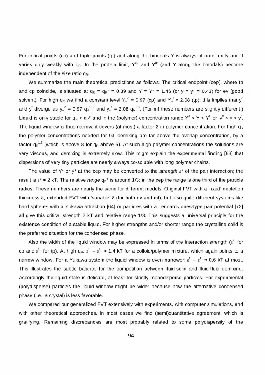
94
For critical points (cp) and triple points (tp) and along the binodals Y is always of order unity and it
varies only weakly with qR. In the protein limit, Ycp and Ytp (and Y along the binodals) become
independent of the size ratio qR.
We summarize the main theoretical predictions as follows. The critical endpoint (cep), where tp
and cp coincide, is situated at qR = qR* = 0.39 and Y = Y* = 1.46 (or y = y* = 0.43) for ev (good
solvent). For high qR we find a constant level Y c = 0.97 (cp) and Y t = 2.08 (tp); this implies that yc
and yt diverge as y c = 0.97 qR1.3 and y t = 2.08 qR
1.3. (For mf these numbers are slightly different.)
Liquid is only stable for qR > qR* and in the (polymer) concentration range Yc < Y < Yt or yc < y < yt.
The liquid window is thus narrow: it covers (at most) a factor 2 in polymer concentration. For high qR
the polymer concentrations needed for GL demixing are far above the overlap concentration, by a
factor qR1.3 (which is above 8 for qR above 5). At such high polymer concentrations the solutions are
very viscous, and demixing is extremely slow. This might explain the experimental finding [83] that
dispersions of very tiny particles are nearly always co-soluble with long polymer chains.
The value of Y* or y* at the cep may be converted to the strength * of the pair interaction; the
result is * 2 kT. The relative range qR* is around 1/3: in the cep the range is one third of the particle
radius. These numbers are nearly the same for different models. Original FVT with a ‘fixed’ depletion
thickness , extended FVT with ‘variable’ (for both ev and mf), but also quite different systems like
hard spheres with a Yukawa attraction [64] or particles with a Lennard-Jones-type pair potential [72]
all give this critical strength 2 kT and relative range 1/3. This suggests a universal principle for the
existence condition of a stable liquid. For higher strengths and/or shorter range the crystalline solid is
the preferred situation for the condensed phase.
Also the width of the liquid window may be expressed in terms of the interaction strength ( c for
cp and t for tp). At high qR, t t 1.4 kT for a colloid/polymer mixture, which again points to a
narrow window. For a Yukawa system the liquid window is even narrower: t t 0.6 kT at most.
This illustrates the subtle balance for the competition between fluid-solid and fluid-fluid demixing.
Accordingly the liquid state is delicate, at least for strictly monodisperse particles. For experimental
(polydisperse) particles the liquid window might be wider because now the alternative condensed
phase (i.e., a crystal) is less favorable.
We compared our generalized FVT extensively with experiments, with computer simulations, and
with other theoretical approaches. In most cases we find (semi)quantitative agreement, which is
gratifying. Remaining discrepancies are most probably related to some polydispersity of the

95
experimental dispersions or to (weak) adsorption [86]. Close to the critical point slight deviations might
be due to the fact that scaled-particle theory, which lies at the basis of (G)FVT, is mean-field like; this
leads to deviations near the critical point [56]. These deviations are not expected to be dramatic for
long-ranged attractions [94].
A particularly interesting aspect is our scaling result y ~ qR1/ along the protein-limit binodals. This
scaling is corroborated by simulations and other theoretical models (although this scaling was not
recognized in the literature published so far). Experimental data for the protein limit are too scarce to
check this scaling experimentally. We hope that our results will lead to more systematic studies in this
direction.
We have presented in this paper not only numerical phase diagrams, but also simple explicit
analytical expressions for critical points, triple points, and binodals. These expressions should enable
experimentalists to plan new experiments, as the parameter range for phase separation follows
directly from these simple equations. In this way it becomes possible to systematically vary the
polymer chain length, the particle radius, and the solvency. This latter aspect could be introduced by
using polymers (e.g., PNIPAM) for which the solvency depends strongly on the temperature.
We formulated theory for either a good solvent or theta conditions. This covers the relevant range
of solvencies almost entirely. Only for solvents on the edge between theta and good solvents (Flory-
Huggins parameter about 0.48-0.49) and for bad solvents ( > 0.5) do we not have a proper
description.
Our generalization of FVT, possible by including the correct dependencies for the depletion
thickness and the osmotic pressure on polymer concentration for interacting chains, shows that free-
volume theory can be modified to describe nonideality. Further extensions to more complex systems
seem possible, as demonstrated recently for charged colloids [95]. It would be challenging to also
include sticky spheres, polymers in a (slightly) bad solvent, and polydispersity effects.

96
Acknowledgements
First of all we are greatly indebted to Sasha Skvortsov for collaboration on analytical theory that
yielded ingredients such as polymer depletion thickness and osmotic pressure as a function of
polymer concentration. This work is published in other papers but constitutes an important basis of
our ‘var’ theory. We thank Henk Lekkerkerker, Dirk Aarts, Frans Leermakers, Christoph Gögelein,
Peter R. Lang, Wilson Poon, Klaas Besseling and Erich Eisenriegler for fruitful discussions and
comments on various aspects of this work. Andrea Fortini and Peter Bolhuis are thanked for providing
computer simulation data. Finally, Martien Cohen Stuart encouraged us to join forces on depletion in
2002, for which we owe him a salute.
References [01] Einstein A. Investigations on the Theory of the Brownian Motion, Dover Publications; 1956. [02] von Smoluchowski, M. Ann Phys 1906; 21:756. [03] Perrin J. Atoms, Constable & Company, London; 1916. [04] Yethiraj A, van Blaaderen A. Nature 2002; 421:513. [05] Levelt Sengers J. How fluids unmix, Edita KNAW, Amsterdam, The Netherlands; 2002. [06] Poon WCK, Pusey PN, Lekkerkerker HNWL. Colloids in suspense, Physics World, 27-32;April 1996. [07] Ilett SM, Orrock A, Poon WCK, Pusey PN. Phys Rev E 1995; 51:1344. [08] Leal-Calderon F, Bibette J, Biais, J. Europhys Lett 1993; 23:653. [09] Faers MA, Luckham PF. Langmuir 1997;15:2922. [10] Meijer EJ, Frenkel D. J Chem Phys 1994;100:6873. [11] Dijkstra M, Brader JM, Evans R. J Phys: Condens Matter 1999;11:10079. [12] Pelissetto A, Hansen J-P. Macromolecules 2006;39:9571 [13] Fuchs M, Schweizer KS. Europhys Lett 2000;51:621. [14] Louis AA, Bolhuis PG, Hansen J-P, Meijer EJ. Phys Rev Lett 2000;85:2522. [15] Sear RP. Phys Rev Lett. 2001;86:4696. [16] Odijk T. J Chem Phys 1997;106:3402. [17] Asakura S, Oosawa F. J Chem Phys 1954;22:1255. [18] Asakura S, Oosawa F. J Pol Sci 1958;33:183. [19] Sieglaff CL. J Pol Sci 1959;41:319. [20] Vrij A. Pure Appl Chem 1976;48:471. [21] de Hek H, Vrij A. J Colloid Interface Sci 1981;84:409. [22] Long JA, Osmond DWJ, Vincent B. J Colloid Interface Sci 1973;42:545. [23] Vincent B, Edwards J, Emmett S, Croot R. Colloids Surf 1988;31:267. [24] Gast AP, Hall CK, Russel WB, J Colloid Interface Sci 1983;96:251.

97
[25] Lekkerkerker HNWL. Colloids Surf 1990;51:419. [26] Lekkerkerker HNWL, Poon WCK, Pusey PN, Stroobants A, Warren PB. Europhys Lett 1992;20:559. [27] Poon WCK. J Phys: Condens Matter 2002;14:R859. [28] Moncho-Jorda A, Louis AA, Bolhuis PG, Roth R. J Phys: Condens Matter 2003;15:S3429. [29] Dijkstra M, van Roij R, Roth R, Fortini A, Phys Rev E 2006;73:041404. [30] Aarts DGAL, Tuinier R, Lekkerkerker HNWL, J Phys: Condens Matter 2002;14:7551. [31] Chatterjee AP, Schweizer KS. J Chem Phys 1998;109:10464; ibid 109:10477. [32] Fuchs M, Schweizer KS. Phys Rev E 2001;64:021514. [33] Fuchs M, Schweizer KS. J Phys: Condens Matter 2002;14:R239. [34] Ramakrishnan S, Fuchs M, Schweizer KS, Zukoski CF. Langmuir 2002;18:1082. [35] Rotenberg B, Dzubiella J, Hansen J-P, Louis AA, Mol. Phys. 2004;102:1. [36] Schmidt M., Fuchs M. J. Chem. Phys. 2002;117:6308. [37] Schmidt M., Denton AR., Brader JM. J. Chem. Phys. 2003;118:1541. [38] Louis AA., Bolhuis PG., Meijer EJ, Hansen J-P. J. Chem. Phys. 2002;116:10547. [39] Louis AA., Bolhuis PG., Meijer EJ, Hansen J-P. J. Chem. Phys. 2002;117:1893. [40] Bolhuis PG., Louis AA., Meijer EJ. Phys. Rev. Lett. 2003;90:068304. [41] Chou C-Y. Vo TTM. Panagiotopoulos AZ. Robert M. Physica A 2006;369:275. [42] Fleer GJ., Tuinier R. Phys. Rev. E 2007;76:041802. [43] Tuinier R., Smith PA., Poon WCK., Egelhaaf SU., Aarts DGAL., Lekkerkerker HNWL., Fleer GJ. Europhys Lett. 2008;82:68002. [44] Schäfer L. Excluded-volume effects in Polymer Solutions, Springer Verlag, Berlin; 1999. [45] Fleer GJ., Skvortsov AM., Tuinier R. Macromolecules 2003;36:7857. [46] Fleer GJ., Skvortsov AM., Tuinier R. Macromol. Theory & Simulations 2007;16:531. [47] Reiss H., Frisch HL., Lebowitz JL., J. Chem. Phys. 1959;31:369. Reiss, H. J. Phys. Chem. 1992;96:4736. [48] Widom B. Science 1967;157,375. [49] Carnahan NF., Starling KE. J. Chem. Phys. 1969;51,635. [50] Hall CK. J. Chem. Phys. 1972;52:2252 [51] Frenkel D., Ladd AJC., J. Chem. Phys. 1984;81:3188. [52] Wood WW, Jacobson JD, J. Chem. Phys. 1957;27:1207. [53] Alder BJ, Wainwright TE, J. Chem. Phys. 1957;27:1208. [54] Hoover WG, Ree FM, J. Chem. Phys. 1968;49,3609. [55] Rowlinson JS., Widom B. Molecular Theory of Capillarity, Clarendon Press, Oxford;1989. Stanley HE. Introduction to Phase Transitions and Critical Phenomena, Oxford University Press; 1988. [56] Vink RLC, Horbach J. J. Chem. Phys. 2004;121:3253. [57] Flory PJ., Principles of polymer chemistry, Cornell University Press, Ithaca, New York; 1953. [58] Eisenriegler E., J. Chem. Phys. 1983;42,1052. [59] Hanke A., Eisenriegler E., Dietrich S., Phys. Rev. E. 1999;59:6853

98
[60] de Gennes P-G. Scaling Concepts in Polymer Physics, Cornell University Press, Ithaca; 1979. [61] Le Guillou JC, Zinn-Justin J. Phys. Rev. Lett. 1977 ;39 :95. [62] Fleer GJ., Tuinier R. Physica A 2007;379:52. [63] M.H.J. Hagen, D. Frenkel, J. Chem. Phys. 101 (1994) 4093. [64] Tuinier R., Fleer GJ. J. Phys. Chem. B 2006;110:20540 [65] Lekkerkerker HNWL. Physica A 1997;244:227. [66] Tejero CF., Daanoun A., Lekkerkerker HNW. Baus M. Phys. Rev. Lett. 1994;73:752. [67] Tang Y., Lu BC-Y. J. Chem. Phys.1993;99:9828. [68] Tang Y., Lin Z-Y., Li Y-G. J. Chem. Phys. 2005;122:184505. [69] Dijkstra M. Phys. Rev. E 2002;66:0214402. [70] Tuinier R., Fleer GJ. Macromolecules 2004;37:8764. [71] Tuinier R., Aarts DGAL., Wensink HH., Lekkerkerker HNWL. Phys. Chem. Chem. Phys. 2003;5:3707. [72] Vliegenhart GJ, Lodge JF., Lekkerkerker HNWL. Physica A 1999;263:378. [73] Ramakrishnan S., Fuchs M., Schweizer KS., Zukoski CF. J. Chem. Phys. 2002;116:2201. [74] Tuinier R., de Kruif CG. J. Chem. Phys. 1999;110:9296. [75] Bolhuis PG., Kofke D. Phys. Rev. E 1996;54:634. [76] Fasolo M., Sollich P. J. Chem. Phys. 2005;122:074904 [77] Fasolo M., Sollich P. J. Phys.: Condens. Matt. 2005;17:797. [78] Lynch I., Cornen S., Piculell L. J. Phys. Chem. 2004;108:5443. [79] Bodnár I., Oosterbaan WD. J. Chem. Phys. 1997;106:7777. [80] Aarts DGAL. J. Phys. Chem. B 2005;109:7407. [81] Annunziata O., Ogun O., Benedek GB. Proc. Natl. Ac. Sci, USA 2003;100:970. [82] de Hoog EHA., Lekkerkerker HNWL. J. Phys. Chem. B 1999;103:5274. [83] Tuinier R., Dhont JKG., de Kruif CG. Langmuir 2000;16:1497. [84] Zhang ZX., van Duijneveldt JS. Langmuir 2006;22:63. [85] van Duijneveldt JS., Mutch K., Eastoe J. Soft Matter 2007;3:155. [86] Wijting WK., Knoben W., Besseling NAM., Leermakers FAM., Cohen Stuart MA. Phys. Chem. Chem. Phys. 2004;6:4432. [87] Bolhuis P.G., Louis AA., Hansen, J-P. Phys. Rev. Lett. 2002;89:128302. [88] Tuinier R. Eur. Phys. J. E 2001;10:123. [89] Paricaud P., Varga S., Jackson G. J. Chem. Phys. 2003;118:8525. [90] Sear RP., Phys Rev E 2002;66:051401. [91] Fortini A., Bolhuis PG., Dijkstra M. J. Chem. Phys. 2008;128:024904. [92] Moussaïd A., Poon WCK., Pusey PN., Soliva MF. Phys. Rev. Lett. 1999;82 :225. [93] Fleer GJ., Cohen Stuart MA, Scheutjens JMHM., Cosgrove T., Vincent B. ‘Polymers at Interfaces’, Chapman & Hall, London, 1993. [94] Fu D., Li, Y., Wu, J. Phys. Rev. E 2003;68:011403. [95] Fortini A., Dijkstra M., Tuinier R. J. Phys.: Condens. Matter 2005;17:7783.

99

Figures: Analytical phase diagrams for colloids and
nonadsorbing polymers
Gerard J Fleer and Remco Tuinier
date: July 9, 2008
1. Introduction
Figure 1.1. GL binodal (dashed), GS binodal (dotted) and FS binodal (solid) for
q=0.4 in a Πv(η) representation. The diamond is the GL critical point, the circles
connected through the horizontal dotted line give the triple point. The demixing
regions are indicated as G + S, G + L, and F + S. Also the one-phase regions for a
fluid (F) and a solid (S) are shown.

Figures: Analytical phase diagrams for colloids and nonadsorbing polymers 2
Figure 1.2. Variation of the critical point (cp) and of the triple point (tp) with the size
ratio q=δ/a. The arrows indicate the direction of decreasing q. The diamond and the
circles (connected by the dotted line) are the same (q = 0.4) as in fig 1.1. The asterisks
correspond to the critical endpoint (cep), where a critical fluid at concentration η∗ (left
asterisk) coexists with a solid at concentration η∗
s (right asterisk); this cep is reached
at q ≈ 1/3. The fluid part of the cep is the endpoint of (the stable part of) the critical
curve. The high-q limit of the triple point is Πv = 6.08, indicated as the dashed line;
the liquid and solid compositions in this limit are equal to the hard-sphere coexistence
concentrations 0.49 and 0.54, respectively.

Figures: Analytical phase diagrams for colloids and nonadsorbing polymers 3
2. Osmotic equilibrium theory
Figure 2.1. A dilute colloidal gas in equilibrium with a concentrated colloidal liquid
and with a reservoir containing only the polymer solution. The depletion layers are
indicated as the grey halo around the particles. In a dilute system only pair interactions
between the particles occur, in a concentrated system multiple overlap of depletion
layers takes place. Throughout this paper the external (reservoir) concentration of
polymer is denoted as ϕ, and the internal concentration in the colloid phases as φ.

Figures: Analytical phase diagrams for colloids and nonadsorbing polymers 4
Figure 2.2. The free volume fraction α as a function of the colloid concentration
η = f/(1 + f) according to eq 2.5, for five values of the size ratio q. The dashed lines
for q = 0.1, 0.2, and 0.4 are the dilute limit (eq 2.2) where the depletion layers do not
overlap.
Figure 2.3. The hard-sphere chemical potentials µ0
f (fluid) and µ0
s (solid) and the
corresponding (pv)0f and (pv)0s as a function of f . The rectangle indicates the FS
coexistence where µ = µ0
0= 15.463 and pv = (pv)0
0= 6.081, at concentrations f0
f =
0.970 and f0
s = 1.185 (or η0
f = 0.492, η0
s = 0.542).

Figures: Analytical phase diagrams for colloids and nonadsorbing polymers 5
Figure 2.4. The functions g (eq 2.21b, solid curves) and h (eq 2.22b, dashed) as a
function of f , for five values of q.
Figure 2.5. The colloid chemical potential µf (eq 2.30; left) and (pv)f (eq 2.31; right)
for a fluid with q = 0.6 as a function of f , for three values of Πv. At Π1v = 2 (lower
curves) there is no phase separation. At Π3v = 2.738 (top curves) a dilute gas (f =
0.052) and a concentrated liquid (f = 0.5) coexist at µ = 7.878 and pv = 2.779: the
coexisting phases are indicated by the small dots. At Πcv = 2.259 (middle) both µ
and p have an inflection point where µ′ = µ′′ = p′ = p′′ = 0: this is the critical point,
indicated by the large dot.

Figures: Analytical phase diagrams for colloids and nonadsorbing polymers 6
3. Phase diagrams for ’fixed q’ in terms of Πv
Figure 3.1. FS binodals for q = 0.2, 0.26, 0.3275 (q∗), 0.35, 0.4, and 0.6. The circles
indicate the triple points for the four highest q values; the triple point for q = q∗ is
the cep. The crosses indicate the high-q (exclusion) limit of the binodals.

Figures: Analytical phase diagrams for colloids and nonadsorbing polymers 7
Figure 3.2. GL binodals for q = 0.3275 (q∗, point binodal), 0.35, 0.4, and 0.6. The
circles for the triple points (and the cep) are the same as in fig 3.1, the diamonds are
the critical points. The plusses indicate the high-q exclusion limit of the GL binodal.
The squares are the two binodal points from fig 2.5.

Figures: Analytical phase diagrams for colloids and nonadsorbing polymers 8
Figure 3.3. Triple points (circles) and critical points (diamonds) for a wide range of
q: q = q∗ = 0.3275 (cep, top), 0.328, 0.33, 0.34, 0.35, 0.36, 0.37, 0.38, 0.4, 0.45, 0.5,
0.6, 0.7, 0.8, 0.9, 1, and 1.2 (this is the standard set from table 5.1). The curves are
analytical approximations: eq 3.18c for the critical curve, eq 3.23 for the gas branch
of the triple curve, and eq 3.21 for the liquid branch. The curve for the solid branch
of the triple point is a simple straight line from (Πv)∗, f∗
s to (pv)00, f0
s .
Figure 3.4. The relation between µ0 and (pv)0 for a hard-sphere liquid (index l) and
a hard-sphere solid (index s). Symbols are calculated from eqs 2.17,18. The curves are
drawn according to eq 3.13 (l) and 3.11 (s).

Figures: Analytical phase diagrams for colloids and nonadsorbing polymers 9
Figure 3.5. The gas branches of three GS binodals from fig 3.1 (q = q∗, 0.35, 0.4)
and of the GL binodal from fig 3.2 for q = 0.6 (solid curves) as compared with the
exclusion limit (dotted): eq 3.14 for GS, eq 3.15 for GL. The circles are triple-point
coordinates, and are the same as in figs 3.1 and 3.2.
Figure 3.6. Normalized colloid concentrations f tg, f t
l and f ts (triangles) for the triple
point and fc (diamonds) for the critical point, and the corresponding Πvt(circles) and
Πvc
(squares), as a function of the inverse (normalized) range 1/q ≡ q∗/q. Symbols
are the numerical data for the same q values as in fig 3.3 (and table 5.1). Curves are
analytical approximations as discussed in the text: eq 3.24 for f tg, eq 3.22 for f t
l , eq
3.20 for f ts, eq 3.19 for Πv
t, and eq 3.18 for fc and Πv
c.

Figures: Analytical phase diagrams for colloids and nonadsorbing polymers 10
Figure 3.7. The gas branch of the triple curve in the representation logf tg as a function
of ζ3. Symbols are the numerical data, the solid curve is eq 3.24, and the dashed line
is the limiting form eq 3.16b.
Figure 3.8. The fluid part of fig 3.3 with triple points (open circles), critical points
(open squares), and GL binodals (solid curves) and spinodals (dotted) for five q values.
Symbols (filled circles for the binodals) are numerical data, the curves are analytical.
The equations for the triple and critical curves (dashed) are given in section 3.2.2, the
binodals (solid) follow eq 3.25 (q = 0.35, 0.4) or eq 3.26 (higher q), and the spinodals
(dotted) are given by eq 3.28. The open diamonds for q = ∞ correspond to the
exclusion limit of eq 3.8, in combination with eq 2.18a.

Figures: Analytical phase diagrams for colloids and nonadsorbing polymers 11
4. Radius of gyration and overlap concentration
Figure 4.1. The linear expansion coefficient αe as a function of the square root of
the chain length for, from bottom to top, v = 0, 0.03, 0.1, 0.2, 0.6, and 1. Symbols
are the numerical solution of eq 4.2, solid curves are the approximation of eq 4.3. The
dotted curve is the high-vn limit αe = 1.10(vn)1/5 for v = 1.
Figure 4.2. The radius of gyration R as a function of the square root of the chain
length for, from bottom to top, v = 0, 0.03, 0.1, 0.2, 0.6, and 1. Symbols are the
numerical solution of eqs 4.1 and 4.2, solid curves follow eq 4.4. The dashed curves are
the scaling relations of eq 4.5.

Figures: Analytical phase diagrams for colloids and nonadsorbing polymers 12
Figure 4.3. The overlap concentration as a function of the solvency parameter v ,
for N = 100, 400, 900. Symbols are numerical data from eqs 4.1, 4.2, and 4.6. Solid
curves follow eq 4.7, dashed curves are the scaling relation eq 4.8b.
Figure 4.4. The overlap concentration as a function of the chain length, for four
values v as indicated. Symbols are numerical data from eqs 4.1, 4.2, and 4.6. The
solid curves are eq 4.7, the dashed curves (v > 0) are the scaling relation eq 4.8b.

Figures: Analytical phase diagrams for colloids and nonadsorbing polymers 13
5. Phase diagrams for ’fixed q’ in terms of the polymer concentration
Figure 5.1. The dependence q0(q) for a theta solvent (dashed curve) and a good
solvent (solid) according to eq 5.3. The symbols are the approximate power-law
behaviour of eq 5.5.
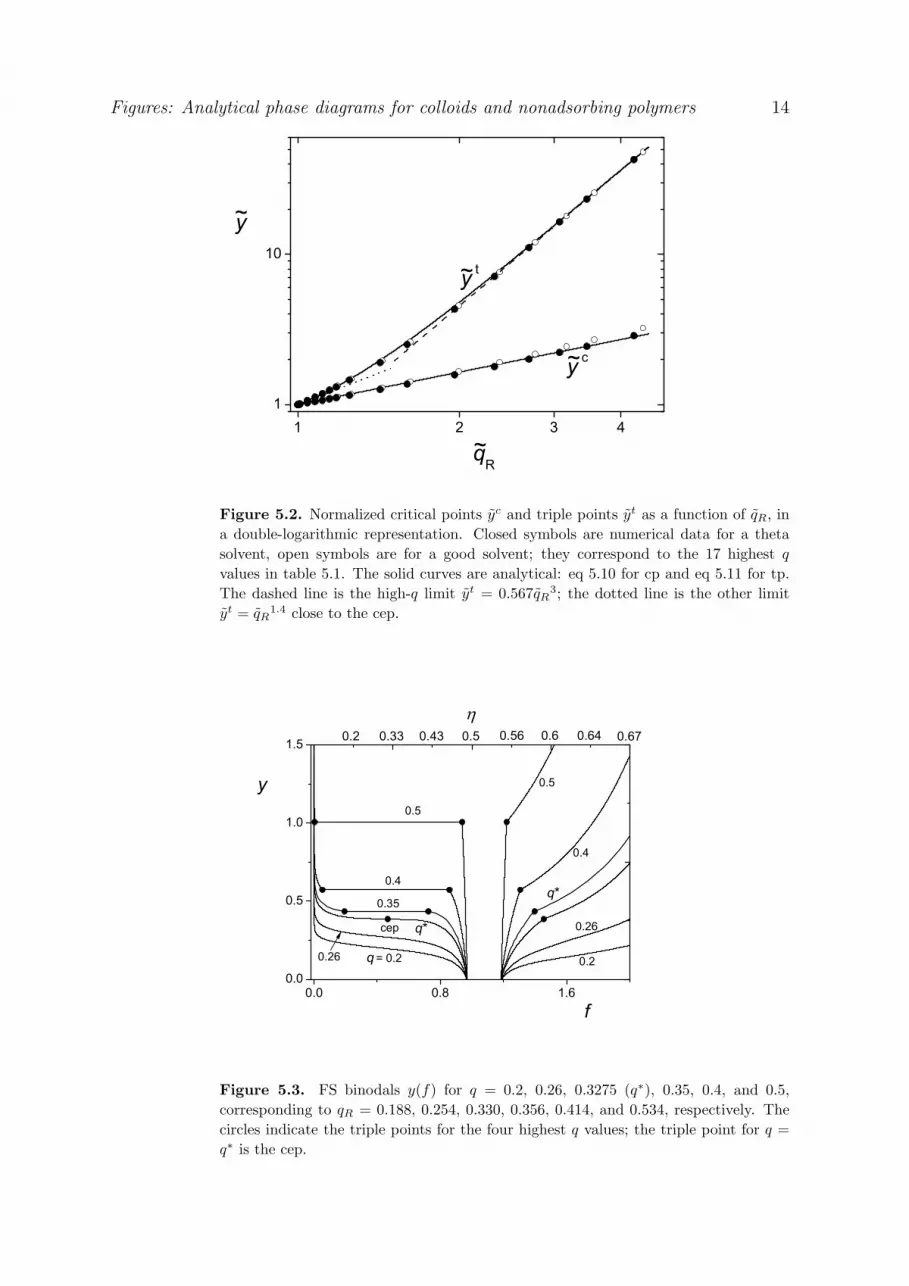
Figures: Analytical phase diagrams for colloids and nonadsorbing polymers 14
Figure 5.2. Normalized critical points yc and triple points yt as a function of qR, in
a double-logarithmic representation. Closed symbols are numerical data for a theta
solvent, open symbols are for a good solvent; they correspond to the 17 highest q
values in table 5.1. The solid curves are analytical: eq 5.10 for cp and eq 5.11 for tp.
The dashed line is the high-q limit yt = 0.567qR3; the dotted line is the other limit
yt = qR1.4 close to the cep.
Figure 5.3. FS binodals y(f) for q = 0.2, 0.26, 0.3275 (q∗), 0.35, 0.4, and 0.5,
corresponding to qR = 0.188, 0.254, 0.330, 0.356, 0.414, and 0.534, respectively. The
circles indicate the triple points for the four highest q values; the triple point for q =
q∗ is the cep.
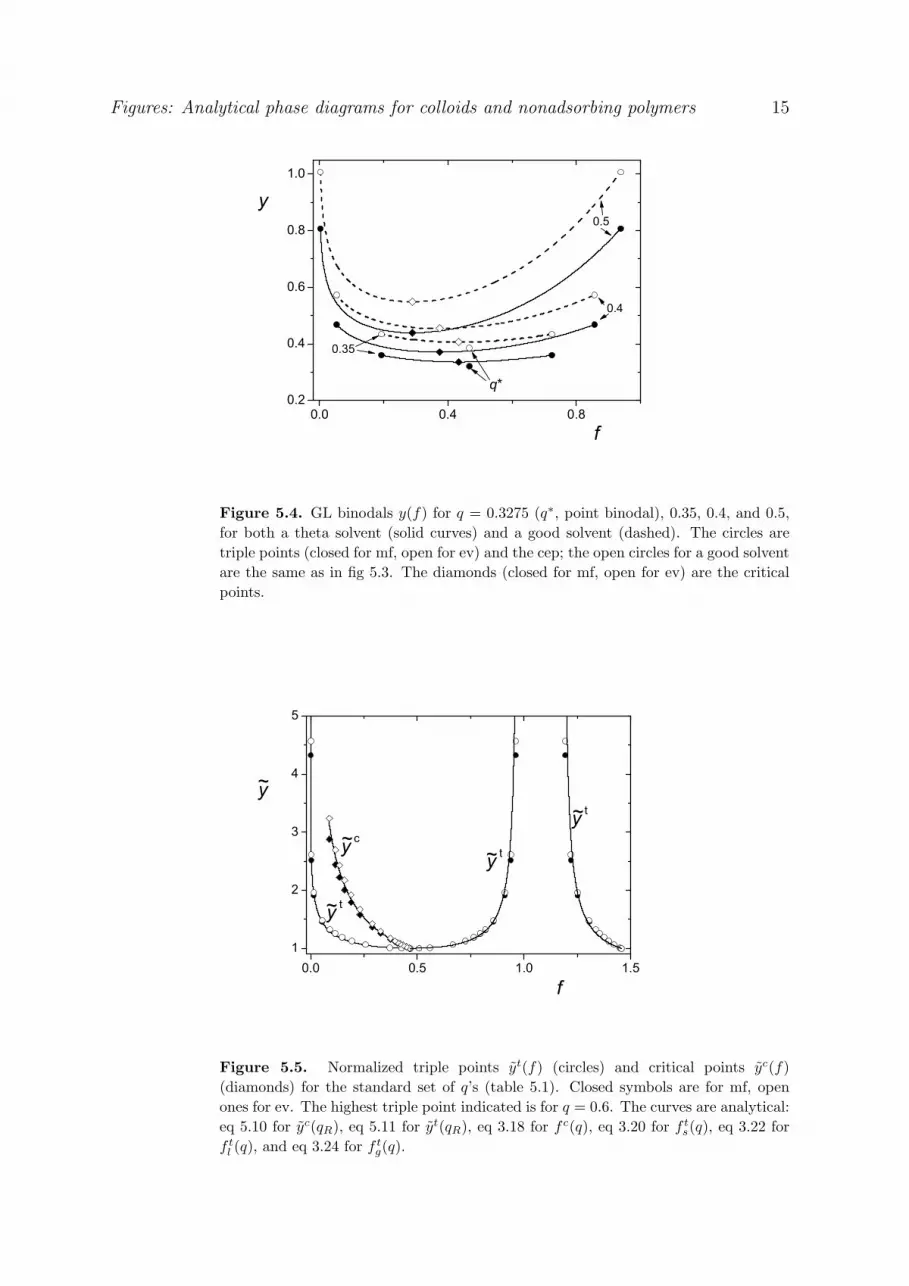
Figures: Analytical phase diagrams for colloids and nonadsorbing polymers 15
Figure 5.4. GL binodals y(f) for q = 0.3275 (q∗, point binodal), 0.35, 0.4, and 0.5,
for both a theta solvent (solid curves) and a good solvent (dashed). The circles are
triple points (closed for mf, open for ev) and the cep; the open circles for a good solvent
are the same as in fig 5.3. The diamonds (closed for mf, open for ev) are the critical
points.
Figure 5.5. Normalized triple points yt(f) (circles) and critical points yc(f)
(diamonds) for the standard set of q’s (table 5.1). Closed symbols are for mf, open
ones for ev. The highest triple point indicated is for q = 0.6. The curves are analytical:
eq 5.10 for yc(qR), eq 5.11 for yt(qR), eq 3.18 for fc(q), eq 3.20 for f ts(q), eq 3.22 for
f tl (q), and eq 3.24 for f t
g(q).

Figures: Analytical phase diagrams for colloids and nonadsorbing polymers 16
Figure 5.6. Normalized phase diagram ϕ(η) for a constant chain length N . Triple
points (circles) and critical points (diamonds) are for the standard set of q’s (table 5.1).
Closed symbols are for mf, open ones for ev. The two GL binodals (dashed curves)
are for q = 0.45 and q = 0.6, the two FS binodals (dotted) are for q = 0.2 and q =
q∗. The four binodals are for a good solvent, but those for a theta solvent would look
essentially the same.
Figure 5.7. Triple points (circles) and critical points (diamonds) for N = 400 and five
solvencies: from top to bottom v = 0, 0.05, 0.1, 0.3, 1, which with eq 4.4 corresponds
to R = 8.2, 10.5, 11.5, 13.7, and 16.9, respectively. The set of q’s is the standard set
(table 5.1). The ϕ∗ values (eq 5.13a) in the cep are 0.056, 0.032, 0.024, 0.014, and
0.0076, respectively. The a∗ values (eq 5.13b) are 26.3, 31.7, 34.9, 41.5, and 51.4.

Figures: Analytical phase diagrams for colloids and nonadsorbing polymers 17
Figure 5.8. Normalized phase diagram ϕ(η) for a constant particle radius a. Triple
points (circles) and critical points (diamonds) are for the standard set of q’s. Closed
symbols are for mf, open ones for ev. The highest triple point indicated is q = 0.6
for mf and q = 0.7 for ev. The GL binodal (dashed curve) is for q = 0.6, the two
FS binodals (dotted) are for q = 0.2 and q = q∗. The three binodals are for a good
solvent, but those for a theta solvent would look essentially the same.
Figure 5.9. Triple points (circles) and critical points (diamonds) for a = 30 and five
solvencies (the same set as in fig 5.7). The set of q’s is again the standard set. The ϕ∗
values in the cep (eq 5.15a) are 0.049 (v = 0), 0.037, 0.030, 0.022, and 0.016 (v = 1).
The R∗ values (eq 5.15b) are 9.3 for v = 0 and 9.9 for v > 0. The corresponding N∗
values (eq 5.15c) are 522 (v = 0), 389, 320, 235, and 168 (v = 1).

Figures: Analytical phase diagrams for colloids and nonadsorbing polymers 18
Figure 5.10. The free volume fraction αt for triple points (tp, open circles) and αc
for critical points (cp, diamonds) as a function of the corresponding colloid volume
fraction ηt and ηc. Symbols are the numerical data for the standard set of q’s (table
5.1). Curves are analytical according to eqs 5.18-21, using the numerical data for
the η’s. The closed symbols and corresponding lines give the normalized quantities
αtl = αt
l/α∗ and αts = αt
s/α∗
s .

Figures: Analytical phase diagrams for colloids and nonadsorbing polymers 19
Figure 5.11. Variation of αt for triple points (tp, three branches) and of αc for critical
points (cp) with 1/q ≡ q∗/q. The gas branch αtg of the triple curve is not normalized
(so it is α∗ in the cep), the other quantities are normalized on the cep. Symbols (circles
for tp, diamonds for cp) are the numerical data for the standard set of q’s (table 5.1).
Solid curves are analytical according to eqs 5.18-21, with the analytical results (eqs
3.18, 20, 22, 24) for the η’s. The dashed curve for αts is eq 5.20 with numerical η’s.
Figure 5.12. Normalized internal concentrations φc (cp, diamonds) and φt (tp,
circles) as a function of qR for a good solvent, on a double-logarithmic scale. Closed
symbols and solid curves are for constant N , open symbols with dashed curves are
for constant a; the symbols correspond to the standard set of q’s (table 5.1). The
normalized φ-values may be converted to real concentrations φ by multiplying with
φ∗ = α∗ϕ∗, where ϕ∗ is given by eq 5.13 (constant N) or eq 5.15 (constant a).

Figures: Analytical phase diagrams for colloids and nonadsorbing polymers 20
Figure 5.13. Normalized phase diagram φ(η) for a constant chain length N and a
good solvent. Three GL binodals (q = 0.35, 0.4, 0.45) are indicated as the dashed
curves. The corresponding triple points are the (nine) circles, the three critical points
are the diamonds. The asterisk is the cep at φ∗ = 1, η = η∗. The triple triangle
connects the three φt, ηt pairs for q = 0.45. The dotted curve is the FS binodal for q
= 0.2.

Figures: Analytical phase diagrams for colloids and nonadsorbing polymers 21
Figure 5.14. Normalized phase diagram φ(η) for a constant particle radius a and
a good solvent. Three GL binodals (q = 0.4, 0.45, 0.6) are indicated as the dashed
curves. Triple points (circles) and critical points (diamonds) are for the standard set
(table 5.1) for q; the highest triple point shown in the G branch is for q = 0.45. The
asterisk is the cep at φ∗ = 1, η = η∗. The triple triangle connecting the three (φt, ηt)
pairs is for q = 0.45. The dotted curves are the FS binodals for q = q∗ and 0.2. The
inset shows more detail for high η; here we omitted the FS binodals.

Figures: Analytical phase diagrams for colloids and nonadsorbing polymers 22
6. Phase diagrams for ’variable q’
Figure 6.1. The dependence q(y)/q(0) on the reduced polymer concentration y =
ϕ/ϕov. Solid curves follow eq 6.17, dashed curves are the semidilute limit q(y)/q(0) =
0.45y−0.9 (mf) or 0.55y−0.68 (ev); these limits are obtained by omitting the unity terms
in eq 6.17.

Figures: Analytical phase diagrams for colloids and nonadsorbing polymers 23
Figure 6.2. The parameters Y c (bottom) and Y t (top) as a function of qR = qR/q∗R.
Symbols (closed for mf, open for ev) are the numerical data, curves (solid for mf,
dashed for ev) are the analytical approximations of eqs 6.26, 27. The numerical data
for mf are qR = q∗R(=0.337), 0.35, 0.4, 0.5, 0.6, 0.7, 0.8, 0.9, 1, 1.2, 1.4, 1.6, 1.8, 2, 3,
4, and 5. Those for ev are the same except for the first three which are q∗R (=0.388),
0.4, and 0.45.
Figure 6.3. Triple points and critical points for ’variable q’ in a Πv(qR) representation.
Symbols and the qR range are the same as in fig 6.2. The curves (solid for mf, dashed
for ev) are analytical approximations, based on eq 6.18 (with Y c and Y t from eqs
6.26,27). The dotted curves are Πvc
and Πvt
for ’fixed q’ (eqs 3.18,19 in combination
with q ∼ q0.88R ).

Figures: Analytical phase diagrams for colloids and nonadsorbing polymers 24
Figure 6.4. Triple points and critical points for ’variable q’ (circles and diamonds)
and for ’fixed q’ (crosses and plusses) in a Πv(f) representation. Closed symbols are
for mf, open ones for ev, for the same qR set as in fig 6.2. The q range for ’fixed q’
is the same as in fig 3.3 and the corresponding qR’s can be read from table 5.1; the
highest q is 1.2, which corresponds to qR = 1.32 (mf) or 1.44 (ev). The curves (solid
for mf, dashed for ev) are analytical approximations, based on eq 6.18 (with Y c and Y t
from eqs 6.26,27) for Πv(qR), and eqs 6.35-38 for ηc(qR), ηtg(qR), ηt
l (qR), and ηts(qR),
whereby the η’s were converted to f using f = η/(1 − η).

Figures: Analytical phase diagrams for colloids and nonadsorbing polymers 25
Figure 6.5. The parameters qc (top) and qt (bottom) as a function of qR = qR/q∗R.
Symbols (closed for mf, open for ev) are the numerical data, curves (solid for mf,
dashed for ev) are eq 6.17 with the analytical approximations of eqs 6.26,27 for Y c and
Y t. The numerical data are for the same qR set as in fig 6.2. The dotted curve is the
’fix’ result q = q0.88R .
Figure 6.6. The parameters yt (circles) and yc (diamonds) as a function of qR, on
a double-logarithmic scale. Closed symbols are for mf, open ones for ev. The curves
(solid for mf, dashed for ev) are the analytical approximations of eqs 6.31,32. For the
top curve (yt for ev) the limiting initial and final asymptotes (yt = qλR and yt = Aqκ
R,
respectively) are indicated as the dash-dotted lines. The dotted curves are yt and yc
for ’fixed q’ according to eqs 5.10,11.

Figures: Analytical phase diagrams for colloids and nonadsorbing polymers 26
Figure 6.7. Numerical data for ηc (diamonds) and for ηtg, ηt
l , and ηts (circles) as a
function of 1/qR. Closed symbols are for mf, open ones for ev. The curves (solid for
mf, dashed for ev) are the analytical approximations of eqs 6.35-38.
Figure 6.8. The free volume fraction αt for triple points (three branches tpG, tpL, tpS,
circles) and αc for critical points (cp, diamonds) as a function of the corresponding
colloid volume fractions ηt and ηc. Symbols (closed for mf, open for ev) are the
numerical data for the standard set of qR’s (see fig 6.2). Curves are analytical according
to eqs 6.41,43 for tpG and tpL, eq 6.45 in combination with eq 6.28 for tpS, and eq
6.39 for cp. The inset shows more detail of the solid part of the triple point.
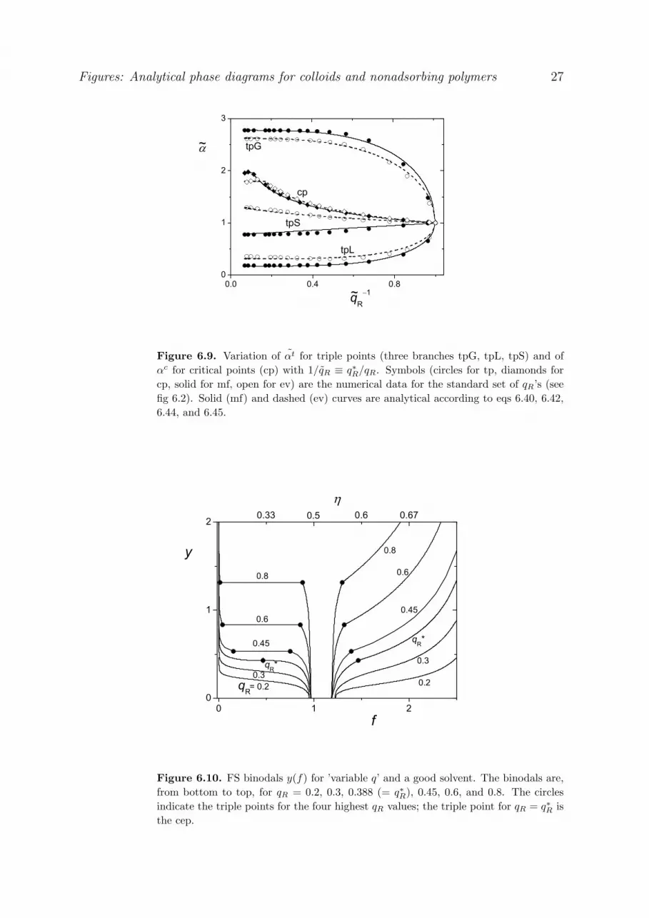
Figures: Analytical phase diagrams for colloids and nonadsorbing polymers 27
Figure 6.9. Variation of αt for triple points (three branches tpG, tpL, tpS) and of
αc for critical points (cp) with 1/qR ≡ q∗R/qR. Symbols (circles for tp, diamonds for
cp, solid for mf, open for ev) are the numerical data for the standard set of qR’s (see
fig 6.2). Solid (mf) and dashed (ev) curves are analytical according to eqs 6.40, 6.42,
6.44, and 6.45.
Figure 6.10. FS binodals y(f) for ’variable q’ and a good solvent. The binodals are,
from bottom to top, for qR = 0.2, 0.3, 0.388 (= q∗R), 0.45, 0.6, and 0.8. The circles
indicate the triple points for the four highest qR values; the triple point for qR = q∗R is
the cep.

Figures: Analytical phase diagrams for colloids and nonadsorbing polymers 28
Figure 6.11. GL binodals y(f) for ’variable q’, for both mf (solid curves, closed
symbols) and ev (dashed, open). The binodals are, from bottom to top, for qR = q∗R(point binodal), 0.45, 0.6, and 0.8. The circles are the (fluid parts of the) triple points,
diamonds are critical points.
Figure 6.12. Normalized triple points yt(f) (circles) and critical points yc(f)
(diamonds) for ’variable q’, for both mf (closed symbols) and ev (open). The range for
qR is the same as in fig 6.2, but the data points for the highest qR values fall outside
the range of the figure: the highest triple points shown are for qR = 1, the highest
critical points are for qR = 2 (mf) and 1.8 (ev). The curves (solid for mf, dashed for
ev) are analytical on the basis of eq 6.31 for yt(qR), eq 6.32 for yc(qR), eq 6.35 for
ηc(qR), and eqs 6.36-8 for the three ηt’s as a function of qR. The η’s in these equations
were converted to f using η/(1 − η).
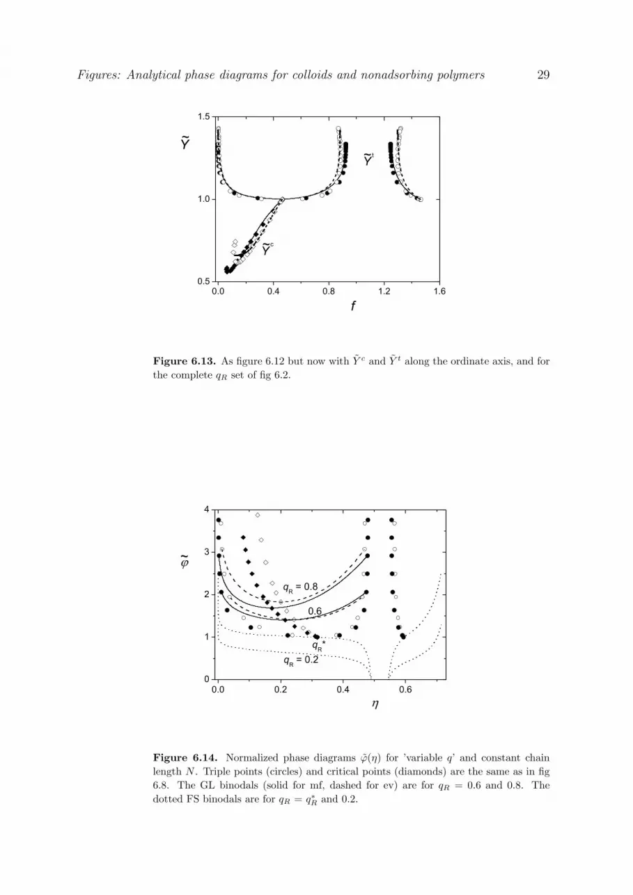
Figures: Analytical phase diagrams for colloids and nonadsorbing polymers 29
Figure 6.13. As figure 6.12 but now with Y c and Y t along the ordinate axis, and for
the complete qR set of fig 6.2.
Figure 6.14. Normalized phase diagrams ϕ(η) for ’variable q’ and constant chain
length N . Triple points (circles) and critical points (diamonds) are the same as in fig
6.8. The GL binodals (solid for mf, dashed for ev) are for qR = 0.6 and 0.8. The
dotted FS binodals are for qR = q∗R and 0.2.

Figures: Analytical phase diagrams for colloids and nonadsorbing polymers 30
Figure 6.15. Triple points (circles) and critical points (diamonds) for ’variable q’
in the representation ϕ(η), for five solvencies and R values (the same as in fig 5.7,
corresponding roughly to N = 400). The qR set is the same as in fig 6.2. The ϕ∗
values (eq 6.3) are 0.053, 0.041, 0.030, 0.017, and 0.0094 for v = 0, 0.05, 0.1, 0.3, and
1, respectively. The a∗ values, given by R/q∗R, are 24.9 (v = 0), 27.1, 29.8, 35.5, and
43.9 (v = 1).
Figure 6.16. Normalized phase diagram ϕ(η) for a constant particle radius a and
’variable q’. Triple points (circles) and critical points (diamonds) are for the same set
of qR’s as in fig 6.2. Closed symbols are for mf, open ones for ev. The two GL binodals
(dashed curves) are for a good solvent and qR = 0.45 and 0.8, the two FS binodals
(dotted) are for qR = 0.2 and qR = q∗R. The FS binodals are for a theta solvent, but
those for a good solvent would look essentially the same.

Figures: Analytical phase diagrams for colloids and nonadsorbing polymers 31
Figure 6.17. Triple points (circles) and critical points (diamonds) for a = 30 and five
solvencies (the same set as in fig 6.15), in the representation ϕ(f) and for ’variable q’.
The qR set is the same as in fig 6.2. The ϕ∗ values are 0.043 (v = 0), 0.035, 0.029,
0.021, and 0.015 (v = 1). The R∗ values are given by aq∗R: 10.1 (mf) and 11.6 (ev).
Figure 6.18. Normalized internal concentrations φc (cp, diamonds) and φt (tp,
circles) as a function of qR for ’variable q’ and a good solvent, on a double-logarithmic
scale. Closed symbols and solid curves are for constant N , open symbols with dashed
curves are for constant a; the symbols correspond to the standard set of qR’s (see fig
6.2). The normalized φ-values may be converted to real concentrations φ by multiplying
with φ∗=α∗ϕ∗, where ϕ∗=y∗ϕov, with ϕov given by 0.87 v−0.28R−1.3 (constant N) or
1.47 v−0.28a−1.3 (constant a).

Figures: Analytical phase diagrams for colloids and nonadsorbing polymers 32
Figure 6.19. Normalized phase diagram φ(η) for a constant chain length N and
’variable q’ in a good solvent. The critical points (diamonds) and triple points (circles)
are for the standard set for qR (see fig. 6.2), but not all these points are in the range
shown: the highest critical point is for qR = 1.2, the highest triple points are for qR
= 0.6 (G), qR = 2 (L), and qR = 5 (S). Three GL binodals (q = 0.45, 0.5, 0.6) are
indicated as the dashed curves. The asterisk is the cep at φ = 1, η = η∗. The triple
triangle connects the three φt, ηt pairs for qR = 0.6. The dotted curve is the FS binodal
for qR = 0.2.

Figures: Analytical phase diagrams for colloids and nonadsorbing polymers 33
Figure 6.20. Normalized phase diagram φ(η) for a constant particle radius a and a
good solvent. Four GL binodals (qR = 0.4, 0.45, 0.6, 0.8) are indicated as the dashed
curves. Triple points (circles) and critical points (diamonds) are for the standard set
(see fig 6.2) for qR. The asterisk is the cep at φ = 1, η = η∗. The triple triangle
connecting the three φt, ηt pairs is for qR = 0.6. The dotted curve is the FS binodal
for qR = 0.2.
Figure 6.21. GL binodals Y (η) for mf and qR = 0.35, 0.5, 1, 3 and 5. Symbols are
the numerical data, curves are the analytical approximations of eq 6.47 (L branch) and
eq 6.48 (G branch). The asterisk is the cep.

Figures: Analytical phase diagrams for colloids and nonadsorbing polymers 34
Figure 6.22. As in fig 6.21 but now for ev and qR = 0.4, 0.5, 1, 4, and 5.
Figure 6.23. The free volume fraction α along the binodals for a theta solvent and qR
= 0.4, 0.6, 0.8, and 5. Symbols are the numerical data, curves are eq 6.51 (G branch)
and eq 6.52 (L branch). The exponent x in eq 6.52 is 1.5 for qR = 0.4 and 0.6, and 2
for qR = 0.8 and 5.

Figures: Analytical phase diagrams for colloids and nonadsorbing polymers 35
Figure 6.24. As fig 6.23 but now for a good solvent and qR = 0.4, 0.5, 0.8, and 5,
with x = 1.5 (L branch).

Figures: Analytical phase diagrams for colloids and nonadsorbing polymers 36
7. The liquid window
Figure 7.1. The dependence of εc (cp) and εt (tp) on qR = qR/q∗R, for both ’fix’
(dashed curves) and ’var’ (solid curves), according to eqs 7.2,3 plus 12. For ’fix’ the
factor 3.77 in eq 7.12 is taken zero.
Figure 7.2. The dependence of εc (cp) and εt (tp) on q = q/q∗, for ’fix’ (dashed
curves), ’var’ (solid curves), and ’Yuk’ (dash-dotted). The latter data are taken from
[64]. The abbreviation Yuk stands for a Yukawa fluid, where 1/k = k∗/k plays the
same role as q.

Figures: Analytical phase diagrams for colloids and nonadsorbing polymers 37
Figure 7.3. The dependence of ϕc (cp) and ϕt (tp) on qR = qR/q∗R for the case of
constant R, for ’fix’ (dashed curves) and ’var’ (solid curves).
Figure 7.4. The dependence of ϕc (cp) and ϕt (tp) on qR = qR/q∗R for the case of
constant a, for ’fix’ (dashed curves) and ’var’ (solid curves).

Figures: Analytical phase diagrams for colloids and nonadsorbing polymers 38
Figure 7.5. The dependence of φc (cp), φtg (tpG), and φt
l (tpL) on qR = qR/q∗R for
the case of constant R, for ’fix’ (dashed curves) and ’var’ (solid curves).
Figure 7.6. The dependence of φc (cp), φtg (tpG), and φt
l (tpL) on qR = qR/q∗R for
the case of constant a, for ’fix’ (dashed curves) and ’var’ (solid curves).
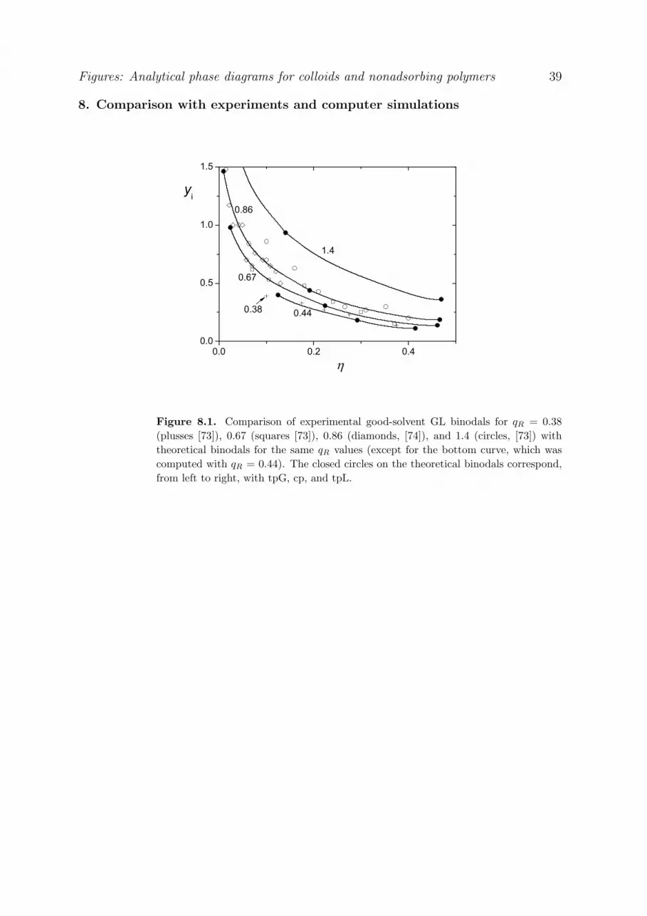
Figures: Analytical phase diagrams for colloids and nonadsorbing polymers 39
8. Comparison with experiments and computer simulations
Figure 8.1. Comparison of experimental good-solvent GL binodals for qR = 0.38
(plusses [73]), 0.67 (squares [73]), 0.86 (diamonds, [74]), and 1.4 (circles, [73]) with
theoretical binodals for the same qR values (except for the bottom curve, which was
computed with qR = 0.44). The closed circles on the theoretical binodals correspond,
from left to right, with tpG, cp, and tpL.

Figures: Analytical phase diagrams for colloids and nonadsorbing polymers 40
Figure 8.2. Comparison of experimental theta-solvent GL binodals for qR = 0.84
(circles, [73]), 1.4 (diamonds, [78]), and 2.2 (squares, [78]) with theoretical binodals for
the same qR values. The closed circles on the theoretical binodals correspond, from
left to right, with tpG, cp, and tpL.
Figure 8.3. Comparison of simulation binodals for qR = 0.67 (crosses, [87]) and 1.05
(plusses, [87]) for excluded-volume chains with theoretical binodals for the same qR
values. The closed circles on the theoretical binodals correspond, from left to right,
with tpG, cp, and tpL.

Figures: Analytical phase diagrams for colloids and nonadsorbing polymers 41
Figure 8.4. Comparison of simulation binodals in the protein limit [40] for qR =
3.86 (crosses), 5.58 (plusses), and 7.78 (diamonds) for excluded-volume chains with
theoretical binodals for the same qR values. Along the vertical axis we did not plot
yi = φ/ϕov (as in fig 8.3) but yiq−1.3R so that all binodals for different qR collapse onto
a single curve. The closed circles on the theoretical binodal correspond, from left to
right, with tpG, cp, and tpL.
Figure 8.5. Comparison of the free volume fraction α for qR = 1.05 from MC
simulations (circles, [91]) with ’variable q’ predictions (solid curve).

Figures: Analytical phase diagrams for colloids and nonadsorbing polymers 42
Figure 8.6. Experimental tie-lines for qR = 0.87 ([81], bottom part) with the
theoretical binodal plus tie-lines (top part) for the same qR. The filled square is the
estimated experimental cp, the open square is the theoretical cp.
Figure 8.7. Phase diagram of a colloid-polymer mixture with qR ≈ 1. Experimental
observations are indicated by open symbols and crosses as listed within the figure.
The theoretical triple triangle according to the ’fixed q’ model (dashed lines) and our
new ’variable q’ model (solid lines) are also shown; filled circles correspond to the
composition of coexisting GLC phases at the ’var’ triple point. The theoretical FC,
GL and GC binodals are indicated as the dashed (’fix’) and solid (’var’) curves, with
the theoretical predictions for the critical point represented by filled squares.
Recommended