
ASSESSMENT OF WELD RESIDUAL STRESS EFFECTS ON
FATIGUE CRACK PROPAGATION IN FERRITIC PRESSURE
VESSEL STEELS
A thesis submitted to The University of Manchester for the degree of
DOCTOR OF PHILOSOPHY
in the Faculty of Engineering and Physical Sciences
2016
CARLOS EFREN JIMENEZ ACOSTA
SCHOOL OF MATERIALS

2
Contents ABSTRACT .................................................................................................................................... 8
Chapter 1. INTRODUCTION ............................................................................................................... 12
1.1 BACKGROUND ........................................................................................................................ 12
1.2 AIM ............................................................................................................................................. 13
1.3 OBJECTIVES ............................................................................................................................. 13
1.4 MOTIVATION ........................................................................................................................... 14
Chapter 2. LITERATURE REVIEW .................................................................................................... 16
2.1 FATIGUE ................................................................................................................................... 16
2.2 RESIDUAL STRESSES GENERATED BY WELDING PROCESS ........................................ 17
2.3 FATIGUE CRACK PROPAGATION IN WELDS .................................................................... 20
2.4 RESIDUAL STRESS EFFECTS IN FATIGUE CRACK GROWTH ....................................... 23
2.4.1 SUPERPOSITION APPROACH ......................................................................................... 23
2.4.2 CRACK CLOSURE APPROACH ...................................................................................... 29
2.5 DIGITAL IMAGE CORRELATION IN FATIGUE CRACK GROWTH ................................. 35
Chapter 3. EXPERIMENTAL METHODS .......................................................................................... 40
3.1 RESIDUAL STRESS MEASUREMENTS ................................................................................ 40
3.2 FATIGUE TEST ......................................................................................................................... 43
3.3 DIGITAL IMAGE CORRELATION ANALYSIS .................................................................... 48
Chapter 4. RESULTS ............................................................................................................................ 52
4.1 RESIDUAL STRESSES ............................................................................................................. 52
4.1.1 RESIDUAL STRESSES RESULTS .................................................................................... 52
4.1.2 RESIDUAL STRESSES DISCUSSION ............................................................................. 60
4.1.3 RESIDUAL STRESS INTENSITY FACTOR, Kres. .......................................................... 65
4.2 DIGITAL IMAGE CORRELATION ANALYSIS .................................................................... 67
4.3 JMAN METHOD ........................................................................................................................ 72
4.3.1 JMAN RESULTS ................................................................................................................ 72
4.3.2 JMAN DISCUSSION .......................................................................................................... 76
4.4 CRACK OPENING DISPLACEMENT METHOD ................................................................... 80
4.4.1 COD RESULTS ................................................................................................................... 82
4.4.2 COD DISCUSSION ............................................................................................................. 97
Chapter 5. CONCLUSIONS ............................................................................................................... 101
5.1 CONCLUSIONS ....................................................................................................................... 101
5.2 FURTHER WORK ................................................................................................................... 103
REFERENCES ............................................................................................................................... 104

3
List of Figures
Figure 2.1: Fatigue failure in an aluminium crank arm (left) and in a turbine blade (right) ..... 16
Figure 2.2: A schematic showing the distribution of residual stresses in a welded plate[4]. .... 18
Figure 2.3: Region of striation growth during fatigue of fine-grained (28 μm) mild steel[15]. 22
Figure 2.4: Intergranular fracture of laser-welded 4130 steel tempered at 300°c for 1 hour .. 22
Figure 2.5: SEM fractograph showing extensive voiding at lath and grain boundaries in aged
9cr-1mo steel[17]. ............................................................................................................... 22
Figure 2.6: Initiation of cavities produced by the formation of cleavage microcracks in the
ferrite phase of cast duplex stainless steel[18].................................................................... 23
Figure 2.7: Off-centre crack[29]. ............................................................................................... 28
Figure 2.8: Possible different crack profiles[23]........................................................................ 30
Figure 2.9: Back face strain (BFS) vs applied load cycle for welded specimen[23]. ................ 32
Figure 2.10: Initial residual stress fields in the FE models by inputting either the measured
stresses or equivalent displacements and comparison with measured data[37][25]. ............ 33
Figure 2.11: CTOD vs load for two distances behind the crack tip[45]. ................................... 36
Figure 2.12: Acquired speckle images of 31x31 mm2 region at various points in time during
crack formation[43]. ........................................................................................................... 37
Figure 2.13: Typical image used in Digital Image Correlation, showing pairs of points in their
original and deformed position[50]. ................................................................................... 38
Figure 3.1: A photograph of the plate prior to removal of a macrograph slice at location
shown for an experiment carried out by Francis et al.[53]. ................................................ 41
Figure 3.2: Measurement points along weld seam and HAZ for both directions: longitudinal
and transverse. .................................................................................................................. 42
Figure 3.3: Measurement locations in plate cut by abrasive disk. ........................................... 42
Figure 3.4: Sample extracted from one weld plate, and electropolished showing the
measurement points. ......................................................................................................... 43
Figure 3.5 : Geometry of SENB4 fatigue specimen. ............................................................... 44
Figure 3.6 : Constant ∆Kappl during the crack propagation for each R-ratio. ........................... 47
Figure 3.7: Set up of the Q-400 System ISTRA 4D. ............................................................... 48
Figure 3.8: Assembly of SENB4 specimen in the Vibrophore machine. ................................ 49
Figure 4.1: Longitudinal residual stresses measured at surface along the weldline. ............... 53
Figure 4.2: Transversal residual stresses measured at surface along the weldline. ................. 53
Figure 4.3: Longitudinal residual stress distribution after cutting an end of the plates. The
measurement was made in transverse to the weld seam. .................................................. 54
Figure 4.4: Transverse residual stress distribution after cutting an end of the plates. The
measurement was made in transverse to the weld seam. .................................................. 54
Figure 4.5: Normal residual stress distribution after cutting an end of the plates. The
measurement was made through the thickness. ................................................................ 55
Figure 4.6: Transverse residual stress distribution after cutting an end of the plates. The
measurement was made through the thickness, in the transverse to weld direction. ....... 55
Figure 4.7: Longitudinal residual stress distribution measured transverse to the weld, for the
single pass weld sample before and after electropolishing. .............................................. 57
Figure 4.8: Transverse residual stress distribution measured transverse to the weld, in
transverse direction, for the sample before and after electropolishing. ............................ 57

4
Figure 4.9: Normal RS distribution measured through the thickness, in normal to the weld
direction, for the plate before cutting and the cut sample after electropolishing process. 58
Figure 4.10: Transverse RS distribution measured through the thickness, in transverse to the
weld direction, for the plate before cutting and the cut sample after electropolishing. .... 58
Figure 4.11 Residual stress intensity factor, Kres, obtained by the Weight Function method. 66
Figure 4.12: Raw images showing the crack behaviour under maximum load, at different
stress-ratios and under different residual stress conditions. ............................................. 67
Figure 4.13: Displacements and maximum normal strains for a=3.0 mm, σres=230 MPa and
R=0.1. ............................................................................................................................... 68
Figure 4.14: Displacements and maximum normal strains for a=3.0 mm, σres=230 MPa and
R=0.3. ............................................................................................................................... 69
Figure 4.15: Displacements and maximum normal strains for a=3.0 mm, σres=230 MPa and
R=0.5. ............................................................................................................................... 69
Figure 4.16: Displacements and maximum normal strains for a=6.0 mm, σres=-280 MPa and
R=0.1. ............................................................................................................................... 70
Figure 4.17: Displacements and maximum normal strains for a=6.0 mm, σres=-280 MPa and
R=0.3. ............................................................................................................................... 70
Figure 4.18: Displacements and maximum normal strains for a=6.0 mm, σres=-280 MPa and
R=0.5. ............................................................................................................................... 71
Figure 4.19: Variation of ∆Kappl and ∆KJMAN as a function of load for a=3.0 mm. ................. 72
Figure 4.20: Variation of ∆Kappl and ∆KJMAN as a function of load for a=3.5 mm. ................. 72
Figure 4.21: Variation of ∆Kappl and ∆KJMAN as a function of load for a=4.0 mm. ................. 73
Figure 4.22: Variation of ∆Kappl and ∆KJMAN as a function of load for a=4.5 mm. ................. 73
Figure 4.23: Variation of ∆Kappl and ∆KJMAN as a function of load for a=5.0 mm. ................. 74
Figure 4.24: Variation of ∆Kappl and ∆KJMAN as a function of load for a=5.5 mm. ................. 74
Figure 4.25: Variation of ∆Kappl and ∆KJMAN as a function of load for a=6.0 mm. ................. 75
Figure 4.26: SENB4 specimen and DIC observation window. ............................................... 80
Figure 4.27: Displacements map in x-direction (ux) showing the COD measurements points 81
Figure 4.28: COD measurement .............................................................................................. 81
Figure 4.29: COD measured in the peak tensile residual stress field. R=0.1, a=3.0 mm. ....... 82
Figure 4.30: COD measured in the tensile residual stress zone. R=0.1, a=3.5 mm. ............... 82
Figure 4.31: COD measured in the tensile residual stress zone. R=0.1, a=4.0 mm. ............... 83
Figure 4.32: COD measured in a residual stress free zone. R=0.1, a=4.5 mm. ....................... 84
Figure 4.33: COD measured in the compressive residual stress zone. R=0.1, a=5.0 mm. ...... 84
Figure 4.34: COD measured in the compressive residual stress zone. R=0.1, a=5.5 mm. ...... 85
Figure 4.35: COD measured in the peak compressive RS field. R=0.1, a=6.0 mm. ............... 85
Figure 4.36: COD measured in the peak tensile residual stress field. R=0.3, a=3.0 mm. ....... 87
Figure 4.37: COD measured in the peak tensile residual stress field. R=0.5, a=3.0 mm. ....... 87
Figure 4.38: COD measured in the tensile residual stress zone. R=0.3, a=4.0 mm. ............... 88
Figure 4.39: COD measured in the tensile residual stress zone. R=0.5, a=4.0 mm. ............... 88
Figure 4.40: COD measured in the compressive residual stress zone. R=0.3, a=5.0 mm. ...... 89
Figure 4.41: COD measured in the compressive residual stress zone. R=0.5, a=5.0 mm. ...... 89
Figure 4.42: COD measured in the peak compressive RS field. R=0.3, a=6.0 mm. ............... 90
Figure 4.43: COD measured in the peak compressive RS field. R=0.5, a=6.0 mm. ............... 90
Figure 4.44: COD measured 0.5 mm behind the crack tip, for R=0.1. .................................... 91
Figure 4.45: COD measured 1.0 mm behind the crack tip, for R=0.1. .................................... 92

5
Figure 4.46: COD measured 2.0 mm behind the crack tip, for R=0.1. .................................... 92
Figure 4.47: COD measured 0.5 mm behind the crack tip, for R=0.3. .................................... 93
Figure 4.48: COD measured 0.5 mm behind the crack tip, for R=0.5. .................................... 93
Figure 4.49: Closure loads extracted from the COD results. ................................................... 94
Figure 4.50: Kclos for R=0.1, R=0.3 and R=0.5. ....................................................................... 95
Figure 4.51: ∆Keff for R=0.1, R=0.3 and R=0.5. ....................................................................... 95
Figure 4.52: FCGR for R=0.1, R=0.3 and R=0.5. .................................................................... 96
List of Tables
Table 3.1 Mechanical properties of SA508 Grade 3 Class 1 (SA508 Class 3 –ASME-) at
room temperature[51]. ........................................................................................................ 40
Table 3.2: Range of loads to generate the required R-ratio and to keep constant ∆Kappl during
the crack extension a. ....................................................................................................... 46
Table 4.1: Presence of noise and plasticity beyond the crack tip. ........................................... 77

6
Nomenclature
a crack length, mm
B specimen thickness, mm
C, m material constants
c, n main fit parameters
E Young’s (elastic) modulus of the material, GPa
F Force, kN
f Newman’s crack opening function
G=Gappl applied strain energy release rate, J/m2
Gres residual strain energy release, J/m2
g(a/W) stress intensity factor function
K=Kappl nominal (or applied) stress intensity factor, MPa√m
Kapplmax máximum nominal (or applied) stress intensity factor, MPa√m
Kapplmin minimum nominal (or applied) stress intensity factor, MPa√m
Kclos closure stress intensity factor, MPa√m
Kcrit critical stress intensity factor, MPa√m
Keff effective stress intensity factor, MPa√m
Keffmax máximum effective stress intensity factor, MPa√m
Keffmin minimum effective stress intensity factor, MPa√m
KJMAN stress intensity factor obtained by JMAN method, MPa√m
Kmax máximum stress intensity factor, MPa√m
Kopen crack opening stress intensity factor, MPa√m
Kres residual stress intensity factor, MPa√m
∆K=∆Kappl nominal (or applied) stress intensity factor range, MPa√m
7
∆Keff effective stress intensity factor range, MPa√m
∆Kth threshold of stress intensity factor range for crack propagation, MPa√m
Loadmax máximum load, N
m Walker exponent associated with stress amplitude
N number of load cycles
p empirical constant describing the curvatures that occur near the threshold FCG
q empirical constant describing the curvatures that occur near the instability reg.
R stress ratio
Reff effective stress ratio
t thickness, mm
Ux Displacement in x-direction.
W specimen width, mm
σ0 maximum tensile residual stress at the center line of welding, MPa
(σamp)max maximum stress amplitude, MPa
(σamp)res residual stress amplitude, MPa
σe endurance limit, MPa
σmax máximum stress, MPa
σmean mean stress, MPa
σres residual stress, MPa
σu ultimate stress, MPa
σyp yielding stress, MPa
ν Poisson’s ratio
ζ normalised coordinate perpendicular to the welding line, mm

8
ABSTRACT
The University of Manchester
Carlos Efren Jimenez Acosta
Doctor of Philosophy
Assessment of weld residual stress effects on fatigue crack propagation in ferritic pressure vessel steels
2016
This project aims to characterize the fatigue behaviour of a crack propagating in a residual
stress (RS) field changing from tension to compression in the welded zone of a ferritic pressure
vessel steel. The fatigue tests were carried out keeping the applied stress intensity factor range
constant to determine the role of residual stresses on fatigue crack growth. The residual stresses
prior to crack growth were evaluated by X-ray diffraction. The weight function method was
used to infer the expected influence of the residual stress on the crack tip in terms of the residual
stress intensity factor.
Two metrics were used to quantify the crack driving force local to the fatigue crack. Firstly the
stress intensity amplitude expressed in terms of the change in the J-integral between maximum
and minimum load and secondly the change in the crack opening displacement COD to
estimate closure stress intensity factor. The displacement fields local to a fatigue crack were
obtained by Digital Image Correlation (DIC) and then analysed by JMAN, an in-house
developed algorithm to extract the J-integral based on finite element method and implemented
using MATLAB® code. The difference between the applied stress intensity factor range and
the effective crack driving force at the crack tip was determined in order to understand the
interaction between the prior residual stresses and crack closure phenomena. Three different
R-ratios were evaluated during the experiment (R=0.1, R=0.3 and R=0.5) in order to quantify
the effect of RS on crack tip stress intensity and crack opening displacement. R-ratio plays a
very important role on the fatigue crack growth rate (FCGR): as R increases, FCGR also
increases. The COD was assessed by means of the displacements obtained by DIC local to the
crack faces. The COD method turned out to be more insightful than the JMAN method for
characterizing the crack propagation, this is due to the presence of plasticity in the ligament
which breaks the non-linear elastic conditions, causing the path-dependence of the J-integral.
The fatigue crack growth rate (FCGR) is influenced to a greater degree by the R-ratio and to a
lesser degree by the residual stress effect. There is a direct relationship between R and FCGR:
as R increases, FCGR also increases, irrespective of the presence of tensile or compressive
residual stresses, with the crack closure showing more tendency to occur at low R (i.e. R=0.1)
than at high R (i.e. R=0.5). The relationship between R and the residual stress effect on FCGR
is inversely proportional: as R increases, the effect of RS decreases; this is, R=0.1 shows more
dependence with respect to the RS field, displaying a combination of crack closure during the
first half of the fatigue cycle with slight crack opening for the rest of it, this when the crack is
extending in the tensile residual stress field. When the crack reaches the compressive RS field,
the presence of crack closure through all the cycle is total, i.e. for a crack length a>5.5 mm.
The influence of compressive residual stresses on R=0.3 and R=0.5 is negligible: the closure
present at the start of the cycle is insignificant so the cracks can be considered as fully open
during the whole fatigue cycle regardless of the residual stress field (tensile or compressive)
in which the crack is growing. Although R=0.3 does not show crack closure, it exhibits a slight
reduction in FCGR as the crack goes into the compressive residual stress field.

9
DECLARATION
The author declares that no portion of the work referred to in the thesis has been submitted in
support of an application for another degree or qualification of this or any other university or
other institute of learning.
COPYRIGHT STATEMENT
i. The author of this thesis (including any appendices and/or schedules to this thesis)
owns certain copyright or related rights in it (the “Copyright”) and he has given The
University of Manchester certain rights to use such Copyright, including for
administrative purposes.
ii. Copies of this thesis, either in full or in extracts and whether in hard or electronic
copy, may be made only in accordance with the Copyright, Designs and Patents Act
1988 (as amended) and regulations issued under it or, where appropriate, in
accordance with licensing agreements which the University has from time to time.
This page must form part of any such copies made.
iii. The ownership of certain Copyright, patents, designs, trade marks and other
intellectual property (the “Intellectual Property”) and any reproductions of
copyright Works in the thesis, for example graphs and tables (“Reproductions”),
which may be described in this thesis, may not be owned by third parties. Such
Intellectual Property and Reproductions cannot and must not be made available for
use without the prior written permission of the owner(s) of the relevant Intellectual
Property and/or Reproductions.
iv. Further information on the conditions under which disclosure, publication and
commercialisation of this thesis, the Copyright and any Intellectual Property and/or
Reproductions described in it may take place is available in The University of
Manchester, in any relevant Thesis restriction declarations deposited in the
University Library, The University of Manchester Library’s regulations and in The
University’s policy on Presentation of Theses.

10
Acknowledgements
First of all, I wish to express my sincere thanks and appreciation to Professor Philip J. Withers
for his support, patience and guidance during the course of this project. Without his supervision
and constant help this thesis would not have been possible. I would like to extend my sincere
gratitude to Professor Andrew H. Sherry for his valuable help in the completion of this thesis.
I also gratefully acknowledge the financial support granted by the Programme for Improvement
of Higher Education Teachers (PROMEP), programme of the Mexican Ministry of Education
(SEP), as well as to the Puebla Institute of Technology (ITP) for its support. Thanks are also
due to Rolls-Royce Marine for the provision of the material for testing.
Last but not the least, I would like to thank my father and my late mother and, particularly, I
wish to express my deepest appreciation to my wife and my sons for their unconditional
support.
Finally, I thank GOD for allowing me to reach the objective of finishing my PhD thesis.

11
CHAPTER
I
INTRODUCTION

12
Chapter 1. INTRODUCTION
1.1 BACKGROUND
When a component can no longer appropriately fulfill the function for which it was designed,
it is said that the component has failed. If this situation happens in a structural component,
which can put human lives in risk, then the scenario can become really catastrophic.
The use of metallic materials in structures has always been associated with a risk of failure.
This can develop through fatigue, brittle fracture, creep or stress corrosion cracking (SCC).
When structures have critical safety applications, failure can result in huge losses, both
financial and human, as well as serious damage to the environment. Although in many cases
failure happens just once in the lifetime of a component, depending on the function of the
component this single failure can result in great catastrophe, for example aircraft crashes, the
burst of big pipelines, the failure of nuclear reactors, or the collapse of large bridges.
Structural integrity analysis has proved to be a powerful tool for analyzing the risk of failure
and assessing the remaining use life of structures. This has become more important in recent
years when financial considerations have led companies to extend the in-service life of
structures beyond their original design life, without increasing risk to human lives.
Structural integrity analysis involves a correct analysis of the stress and strain the component
is subjected to, an understanding of materials behavior under these conditions and knowledge
of failure mechanisms, as well as the interaction between these issues. The development of
advanced numerical and experimental techniques has improved the structural integrity
assessment methods and made it more reliable.
The main threat for the mechanical integrity of structures is fatigue. Extensive studies have
examined fatigue failures due to the fact that they can occur in normal service when cyclic
loading is present, i.e., without excessive overloads. Fatigue is a process of progressive
fracture, in which a component subject to cyclic loads develops a crack which grows until
reaching a critical size which causes the final fracture of the element.
The welding process used for joining metallic elements during manufacture and/or assembly,
introduces residual stresses in the vicinity of the weld. These stresses, depending on if they are

13
compressive or tensile, improve or diminish, respectively, the fatigue strength on the welded
joint.
Regardless of the cause, the appearance and propagation of fatigue cracks in a residual stress
field is an undesirable event. The role of the residual stresses on the fatigue crack growth is an
issue that must be analysed and understood in order to have more accurate and reliable
predictive models for structural integrity assessments. This understanding can help to avoid
these assessments becoming over-conservative, with tendency to use unnecessary safety
margins and/or early retirement of the element, or under-conservative, which can have tragic
consequences for society and for environment through the premature failure of the welded
component.
1.2 AIM
The aim of this thesis is to characterize the fatigue behaviour of a crack propagating in a
residual stress field changing from tension to compression in the welded zone of a ferritic
pressure vessel steel.
1.3 OBJECTIVES
1. To characterize the residual stress field of a SA508 Grade 3 Class 1 ferritic steel sample
via X-ray diffraction.
2. To examine a fatigue crack propagating within a residual stress field during a fatigue
test using Digital Image Correlation (DIC).
3. To assess the residual stress contribution to the stress intensity factor (Kres) along the
crack path using the weight function method.
4. To obtain the effective crack driving force (ΔKeff) at the crack-tip as it propagates
through the residual stress field using the J-integral method to analyse the displacement
field, obtained from DIC.
5. To quantify the extent of crack residual stress induced crack closure during crack
propagation by evaluating the crack opening displacement (COD) in the vicinity of the
crack tip as it propagates through a residual stress field.
14
1.4 MOTIVATION
The knowledge of fatigue crack growth behaviour in a residual stress field is of practical
interest for many applications, mainly in those that involve the risk of loss of human lives
and/or huge financial loses, examples of these include oil rigs, power plants, airplanes, bridges.
Nowadays, welding is the most commonly used method for joining metallic components but,
paradoxically, welding is the main cause of residual stresses in metallic structures. Residual
stresses are generally considered detrimental for the integrity of structures but there are cases
that indicate the contrary. Whatever the case, the real influence of residual stress on fatigue
crack growth should be accurately determined in order to avoid over-conservative or,
otherwise, under-conservative structural integrity assessments, either of which could have a
negative impact on the industrial sector. The results from this research should enable more
accurate and reliable predictive models for the structural analysis of nuclear pressure vessels
to be produced. By extending the safe operational lifetime of the vessel beyond its original
design life will save costs whilst maintaining safety in order to prevent loss of life and risks for
the environment.

15
CHAPTER
II
LITERATURE
REVIEW

16
Chapter 2. LITERATURE REVIEW
2.1 FATIGUE
Fatigue is a process of progressive fracture. A body subjected to cyclic loads develops a crack
which grows slowly until it reaches a critical size at this point the element undergoes sudden
failure and it fractures. Figure 2.1 shows two examples of progressive failure due to fatigue,
the two stages of this failure process can be clearly distinguished: slow crack growth (dark
area) and sudden fracture (bright area).
Figure 2.1: Fatigue failure in an aluminium crank arm (left) and in a turbine blade
(right). Images retrieved from:
http://upload.wikimedia.org/wikipedia/commons/thumb/9/96/Pedalarm_Bruch.jpg/220
http://www.engelmet.com/images/img_turbine.jpg
Despite extensive research and dissemination over many decades, fatigue remains the most
common mode of failure in structural and mechanical components. Joints in structural members
are particularly susceptible and have poor fatigue performance[1].
The same is true of welded structures: weld joints are more prone to fatigue failures than base
metal, even if the latter contains stress concentration elements. For this reason, fatigue analyses
are of high practical interest for all cyclic loaded welded structures.

17
2.2 RESIDUAL STRESSES GENERATED BY WELDING PROCESS
Welds are a major source of detrimental tensile residual stresses. They are therefore a frequent
source of fatigue failures. Formation of the residual stress in weldment can be attributed to
three sources: the non-uniform simultaneous heating and cooling of the part during welding,
variation in shrinkage due to variable cooling rates in different regions of the weldment (surface
cooling effects), and the volumetric changes during metallurgical phase transformations;
hence, they are unavoidable with the welding process[2]. The cause and effect of each of these
factors will be discussed in more depth:
Differential heating and cooling. As heat source comes close to the point of interest,
its temperature increases, creating a Heat Affected Zone (HAZ)1. The increase in
temperature decreases the yield strength of material and causes thermal expansion of
the heated weld metal. The expansion in the HAZ is limited by the lower temperature
of the base metal which causes a compressive strain to develop within the metal during
heating. When the heat source moves away from the point of interest the temperature
in the HAZ begins to decrease. This causing the HAZ to shrink but the weld metal
cannot freely contract so it remains in a strained condition. This generates tensile
residual stresses along the weld[3]. The differential heating and cooling during welding
generates tensile stress along with weld and compressive stresses in the adjacent HAZ
and base metal. The residual stress experienced caused by welding is a balance between
the tensile and compressive stresses as shown in Figure 2.2.
Differential cooling rate in different zone. Immediately after welding, the cooling
rate at the top and bottom surfaces of weld joint is higher than that experienced in the
core/middle portion of weld and in the HAZ. This causes differential expansion and
contraction through the thickness of the plate being welded, which leads to the
development of compressive residual stresses at the surface and tensile residual stresses
in the core[3].
1 The HAZ is the area of base material which is not melted and has had its microstructure and properties altered by welding. The heat from the welding process and subsequent re-cooling causes this change from the weld interface to the termination of the sensitizing temperature in the base metal.

18
Figure 2.2: A schematic showing the distribution of residual stresses in a welded plate[4].
Solid-state phase transformation. There have been many advances in the evaluation
of welding residual stresses in austenitic stainless steel. However, due to the
complexities associated with the solid-state phase transformations that occur during
welding there has been less progress in understanding the case of ferritic steels. The
deformations associated with solid-state deformations in ferritic steels can have a
significant effect on the weld residual stresses. The transformation can also affect the
misfit strain between weld and parent plate through transformation plasticity[5].
There are two main types of transformation[6]: displacive or reconstructive. The
displacive transformation is where the new structure is produced by a deformation of
the parent crystal, and the reconstructive transformation involves the uncoordinated
diffusion of all the atoms. Both mechanisms cause substantial strains within the
material. The reconstructive transformations cause a volume change which is, in
general, isotropic, whereas displacive transformations involve a combination of a shear
and a dilatational strains. These transformation strains can be very large, greatly
exceeding elastic strains.
The typical residual stress distribution for most of steels comprises of tensile stresses
at weld metal and compressive stresses in the base metal, with an unsteady

19
tensile/compressive residual stress over the HAZ. However, the stress distribution in
ferritic steels does not follow the abovementioned pattern due to the occurrence of
solid-state phase transformations in the weld metal and HAZ during cooling. The
transformational strain counteracts and eventually overwhelms the thermal contraction
strain, generating a noticeable decrement in tensile stress values. Even if the
transformation temperature decreases enough to prevent the accumulation of
contraction stresses once the phase transformation has finished, is very likely that the
tensile stresses characteristic of the HAZ will still turn into compressive stresses.
Residual stresses may be minimized by the choice of joint design, welding technique and post
weld heat treatment (PWHT), but they cannot be eliminated. Several experimental methods are
available for determining residual stresses. They include X-ray diffraction, neutron diffraction,
surface and deep hole drilling, boring, slicing and magnetic methods.
Residual stresses can have a significant influence on the fatigue lives of engineering
components[7][8]. Under fatigue loading conditions, residual stresses do not cycle as the applied
loads cycle, they are effectively “static”. This means that they do not directly influence the
amplitude of the in-service cyclic loading, but they do influence the mean or maximum value
of the load in each cycle. The fatigue nucleation life (the number of cycles required to form
fatigue microcracks) is a function of the alternating stress amplitude but not the mean stress,
while the growth rates of fatigue cracks are a function of both the stress amplitude and the
mean stress. This implies that residual stresses have relatively little influence on fatigue crack
nucleation, but potentially a significant influence on fatigue crack growth rate[9].
This is further complicated as that the initial residual stress field inherent in a metal or induced
by the manufacturing process (including welding) may not remain stable throughout the service
life. The residual stresses can relax and redistribute due to a variety of mechanisms. A single
applied load that causes yielding in a region of residual stress (due to the superposition of
residual and applied loads of the same sign) will result in changes in the residual stresses upon
removal of the applied load. Repeated cyclic loading can also cause gradual changes in the
residual stresses over time, even if no single fatigue cycle induces local yielding. Exposure to
elevated temperatures can also relax residual stresses by creep deformation. Finally, extension
of a fatigue crack through an initial residual stress field can cause significant changes in the

20
residual stress field under some conditions. The specific mechanisms are different for each of
these different effects, and the various effects often superimpose[9].
In the high stress range, the magnitude of residual stresses does not affect the fatigue strength
because residual stress is relaxed during the early fatigue cycles. At the low stress range, fatigue
strength depends on the initial residual stress because residual stress hardly changes by fatigue
loading. It is thought that the relaxation behaviour of residual stress is determined by the
presence of plastic deformation in the weld toe during fatigue cycling[10].
2.3 FATIGUE CRACK PROPAGATION IN WELDS
In order to analyze the fatigue process in a welded joint it is necessary to calculate the value of
the Stress Intensity Factor (SIF) of the fatigue crack.
Maddox[11], in 1975, collected together the various SIF solutions and adapted them to the
particular case of a semi-elliptical surface and through-thickness crack at the toe of a fillet
weld. The influence of the weld as a stress concentration feature was incorporated in the
solution using Finite Element Analysis (FEA). This approach provided results and estimates
based on the stress concentration factor of the uncracked joint.
Most investigations on Fatigue Crack Growth Rate (FCGR) have used specimens having crack
directions parallel to the weld seam. These studies have shown that the locus of the crack path,
material, welding process and heat input do not affect markedly the crack growth rate response.
Nicoletto[12] tested multi-pass butt-welded joints in the through-thickness direction of a mild
steel specimen, in order to obtain FCGR properties. He observed optically the crack length and
computed the FCGR by means of an incremental seven point method. The crack closure
phenomenon was investigated with the unloading elastic compliance technique. Nicoletto[12]
concluded that, for the base material, the observed insensitivity to positive R-ratios was
associated with the prevailing plane strain conditions and the bending specimen geometry,
which reduced the effect of plasticity-induced crack closure, whereas for the multi-pass butt-
welded joints the FCGR depended on R-ratio and propagation direction.
The size of the cracks is the key information used during in-service inspection to assess the
structural integrity of a component. Although the crack depth is the controlling variable for
fatigue analysis, both the depth and length of the surface breaking cracks are needed to assess

21
the remaining capacity of a component. Traditional fatigue design is based on S-N (stress-life)
analysis but this approach does not provide crack growth information for the joints. Fracture
mechanics methods are preferred for in-service integrity assessment.
By the beginning of 1970’s, several researchers had reached the conclusion that a fatigue crack
is diverted toward the softer material in specimens containing a hard HAZ induced by welding.
Richards and Lindley[13] made some observations which related fatigue crack propagation to
microstructure (including weld metals):
a) Low strength alloys propagate by a striation mechanism (Figure 2.3).
b) Tempered martensitic structures tend to exhibit intergranular separation at low ΔK
values (Figure 2.4) and void coalescence at high values of ΔK (Figure 2.5).
c) Materials with brittle second phase particles tend to be associated with microcleavage
(Figure 2.6).
Furthermore, the microstructure of the HAZ depends on the steel composition and the thermal
history of the weld. In multi-pass welding, the microstructures of the coarse-grained HAZ
(CGHAZ) formed in the initial thermal cycle will be refined by subsequent welding passes.
Tsay et al.[14] studied the role of microstructures on the fatigue crack growth of EH36 TMCP
(thermo-mechanical control process) steel weldments, measuring the FCGRs of the steel plate
as well as the HAZ. The FCGRs reduced as the crack propagated into the HAZ and then
eventually entered into the BM (base metal). The lower FCGRs of the HAZ than those of the
steel plate was attributed to the microstructure, i.e. the formation of low-carbon bainite with
high toughness. Transgranular fatigue fracture with fatigue striations at high ΔK values was
observed for all the (CT) Compact-Tension specimens. The tempered HAZ specimens, with
slightly tougher microstructures, possessed lower FCGRs at high ΔKs. In addition, the
existence of compressive residual stresses in the HAZ enhanced the crack closure, resulting in
reduced crack growth rates at low ΔKs.

22
Figure 2.3: Region of striation growth during fatigue of fine-grained (28 μm) mild steel.
ΔK = 30 MNm-3/2. (Arrow indicates general direction of crack propagation)[15].
Figure 2.4: Intergranular fracture of laser-welded 4130 steel tempered at 300°C for 1
hour[16].
Figure 2.5: SEM fractograph showing extensive voiding at lath and grain boundaries in
aged 9Cr-1Mo steel[17].

23
Figure 2.6: Initiation of cavities produced by the formation of cleavage microcracks in
the ferrite phase of cast duplex stainless steel.The bar indicates a scale of 15 μm[18].
2.4 RESIDUAL STRESS EFFECTS IN FATIGUE CRACK GROWTH
There are two methods for evaluating fatigue strength in materials containing residual stress
fields: fracture mechanics and fatigue strength curve. Fracture mechanics uses the principle of
elastic superposition, and this method analyzes the SIF due to the initial residual stress and the
effects of residual stress are evaluated as a change of stress ratio. Adams[19], in 1973, was
amongst the first to propose a simple superposition approach using weight function methods to
determine the net effect of residual stresses and applied loads on FCGR in welded joints[9].
There are two subsidiary methods that use fracture mechanics to evaluate fatigue strength: one
uses the redistribution of residual stress caused by crack propagation[20][21] and the other uses
the effective stress intensity factor range due to crack closure[22][23]. When a fatigue strength
curve is used, the residual stress is treated as a mean stress[10].
2.4.1 SUPERPOSITION APPROACH
The approach employed most frequently to account for the effect of residual stress on fatigue
crack growth involves superposition of the respective SIF for the initial residual stresses and
for the applied stresses. Given that the SIF is derived from a linear elastic analysis, the
superposition principle will apply. This states that the stress system due to two or more loads

24
acting together is equal to the sum of the stresses due to each load acting separately. An
“effective” SIF (Keff) is then taken as:
resappleff KKK (2.1)
where:
Keff = effective stress intensity factor, MPa√m
Kappl = nominal (or applied) stress intensity factor, MPa√m
Kres= residual stress intensity factor, MPa√m
Kres is usually obtained by using Weight Function solution by applying the residual stress field
to the uncracked component. However, this Weight Function technique gives only qualitative
results for structures that are not according with elementary cases. In order to achieve a more
accurate determination of Kres the residual stress distribution has to be known at each stage of
the crack growth[24].
The incorporation of residual stresses using the mean stress approach assumes that the range
of Keff does not change when the residual stresses are superimposed:
applapplapplresapplresappleff KKKKKKKK minmaxminmax (2.2)
where:
∆Keff = effective stress intensity factor range, MPa√m
Kapplmax = maximum nominal (or applied) stress intensity factor, MPa√m
Kapplmin = minimum nominal (or applied) stress intensity factor, MPa√m
∆Kappl = ∆K = nominal (or applied) stress intensity factor range, MPa√m
However, the local stress ratio Reff will continually change as the crack propagates through the
superimposed residual stress field for a constant R-ratio, and hence will cause a mean stress
alteration at the crack tip as:
,max
min
appl
appl
K
KR
resappl
resappl
eff
eff
effKK
KK
K
KR
max
min
max
min
, RReff (2.3)
where:

25
R = stress ratio
Reff = effective stress ratio
Keffmax = maximum effective stress intensity factor, MPa√m
Keffmin = minimum effective stress intensity factor, MPa√m
This indicates that the models for crack growth should include the effective stress ratio in
addition to the stress range, i.e. the Forman equation[24]:
eff
m
R
KC
dN
da
1 for R > 0 (2.4)
eff
m
eff
R
KC
dN
da
1 for R < 0 (2.5)
where:
a = crack length, mm
N = number of load cycles
C, m = material constants
Also, the stress intensity factor can be derived by:
GEK (plane stress) 21
GE
K (plane strain) (2.6)
The relation between K and G only holds for the linear elastic material behaviour.
Superposition has been widely used in the framework of linear elastic fracture mechanics
(LEFM), especially when the weight function method (WFM) is employed to estimate Kres,
Two separate analyses are necessary to find the Kappl and Kres and then the K[25]:
resappl KKK (2.7)
The calculations of G and K can be performed separately for both externally applied and
internal residual stress fields.
The strain energy release rate is commonly calculated by Finite Element Method (FEM) using
schemes based on node forces[26]. In this particular case, by applying the respective stress field

26
to the same FEM model, Gappl and Gres can be found by means of the modified virtual crack
closure technique (MVCCT) using the equation:
)(2
1 *
, jjiyyFat
G
(2.8)
where:
Fyy,i = nodal reaction force perpendicular to the crack growth path at the crack tip node i
(νj-νj*) = crack opening displacement at node j immediately behind the crack tip
∆a = crack extension length that equals to the crack tip element size
t = plate thickness
and then Kappl and Kres be calculated by Equation (2.6) for the respective stress fields[25],
assuming linear elastic conditions.
Under cyclic loads, only Reff changes due to the presence of residual stresses. It is worth noting
that Reff is not the same as the nominal applied stress ratio R. The Walker, Harter T-method,
and NASGRO equations were used in this analysis to calculate FCGR using Reff to replace the
nominal R-ratio in the original equations.
Considering the welding residual stress effect such equations are expressed as the Walker
equation, (2.9) or the NASGRO equation (2.10)[25]:
nm
resappl
appl
applKK
KKC
dN
da
)1(
max,
Walker (2.9)
q
crit
resapp
p
app
thn
app
eff
K
KK
K
K
KR
fC
dN
da
max,1
1
1
1 NASGRO (2.10)
FCGR of the welded sample was significantly higher than that of the base material due to the
presence of tensile residual stresses. Overall the NASGRO equation gives a better prediction
than the Walker equation.
27
The Walker equation does have an appealing advantage for predicting FCGR in residual stress
fields. All one needs to have is a set of measured da/dN data for two different R-ratios for the
base material. The limitation of the Walker equation is that it is too simplistic and it
underestimates the final part of the FCGR when the SIF approaches the material fracture
toughness. NASGRO provides better predictions because it considers the effect of plasticity
induced crack closure by an empirical constant f, and it also takes account of the final fast crack
growth stage when Kmax approaches Kcrit. For materials where the NASGRO equation
coefficients are unknown, the Harter T-method (which is a modified version of the Walker
equation) can be a good prediction tool.
The Walker equation predicts much slower FCGR compared to the other two methods.
Servetti and Zhang[25] concluded that tensile residual stresses (acting like a mean stress) reduce
crack closure effect and increase FCGR. This effect is most pronounced for lower nominal R-
ratios than for higher R-ratios as the influence of Kres on FCGR is small.
In a supplemental discussion to a previous paper by Terada[27] for essentially the same problem
(analysis of SIF for a crack perpendicular to a welding bead), Tada and Paris[28] showed that it
is valid to obtain values of crack-tip stress intensity, arising from a residual stress distribution,
by superposition of the residual stress field onto the crack geometry in a weld. They chose a
different function f(ξ) to represent the residual stress distribution, compare Equations (2.11)
Terada’s choice and (2.12) Tada and Paris’ choice:
)1()( 22
1
1
2
ef Terada choice (2.11)
4
2
21
1)(
f Tada and Paris choice (2.12)
The SIF remained always positive even when the crack extended well into the compressive
stress region. This suggests that the most convenient form for the final expression of K2 would
be:
c
aFaK 202 (2.13)

28
where c is the location of the point of stress reversal. The term a 0 in this expression
represents the SIF for a crack in an infinite plate under uniform tension σ0. F2(a/c) can be
evaluated as:
2/1
4
24
2
1
1
c
a
c
a
c
a
c
aF (2.14)
Later, Terada and Nakajima[29] carried out a similar analysis to the previous with the only
difference that the crack was off-centre. In the Figure 2.7, σ is the original residual stress
distribution without a crack, σ0 is the maximum tensile residual stress at the center line of
welding, ζ is the coordinate perpendicular to the welding line normalized by the characteristic
length where the stress distribution changes from tension to compression and 2a is the crack
size.
They found that, for a constant crack length, the maximum SIF does not occur when the crack
center coincides with the welding line, but does when the crack front approximately reaches
the welding line. It should be noted here that the original residual stress distribution form is no
longer preserved near the crack when the crack exists because of stress re-distribution due to
crack extension.
LaRue and Daniewicz[30] used elastic superposition to predict a fatigue crack growing in a
residual stress field. The implementation of the method is simple and the results are relatively
accurate. However it is possible to increase the accuracy by using a closure-based approach,
but this increases the complexity of the model.
Figure 2.7: Off-centre crack[29].
σ/σ0
ζ

29
2.4.2 CRACK CLOSURE APPROACH
A growing fatigue crack will also generate its own residual stress field, both in front of and in
the wake of its tip. The compressive residual stresses left in the wake influences the crack
closure phenomenon (an effect noticed by Elber[31][32]), which has provided an explanation for
such effects as crack growth retardation caused by periodic high tensile loads and the transient
acceleration caused by low-to-high load transitions.
Unlike the mean stress approach, the crack closure approach can take into account the
compressive residual stresses. The superimposed Kres can either decrease or increase Keff
depending on the sign of Kres and the crack can only propagate if the crack tip experiences
tensile mode-I opening condition, i.e. Keff > 0. Considering constant R-ratio, only part of the
crack will be open if Keff > 0 and closed if Keff < 0.
Numerous researchers have proposed that a crack closure approach is a superior means of
addressing residual stress effects on crack growth in weldments[21][33][34][35]. This approach
assumes that the residual stress field influences the crack opening stress (i.e. the stress at which
the fatigue crack tip first becomes fully open during the loading cycle), and that the resulting
changes in the effective stress intensity factor range correlate with changes in the FCGR. The
crack opening levels are determined using either experiment or analysis, Miyamoto et al.[33]
focused his pioneering work in FEA of fatigue crack closure on the welding problem, and
Fukuda and Sugino[34] employed a similar numerical approach to predict how welding residual
stresses influenced crack opening behaviour[9].
Nelson[21] compared both approaches: superposition and crack closure.
The superposition approach has been used to predict FCGR of cracks in existing residual stress
fields under constant amplitude loading. The closure model has been used to predict load
sequence and mean stress effects in specimens with crack-generated residual stress fields.
A simplified crack closure model that considers residual stress redistribution with crack
extension generates more realistic predictions of FCGR behaviour than the superposition
approach and provides somewhat better predictions of the same parameter than Glinka’s
method for cracks growing first through residual tension, and on into residual compression[21].

30
The crack closure approach provides the mechanics to account for the influence of pre-existing
residual stress fields on growth behaviour, including changes in stress fields due to service
loadings and crack growth, but has not been used significantly for that purpose.
The primary drawback of the crack closure approach is that it usually requires elastic-plastic
FEA, which must be repeated as a crack grows. Simplified closure models (for example, based
on the Dugdale model) are available to reduce that computational burden, but their applicability
is currently limited to simpler crack geometries, such as center-cracked sheets.
The superposition approach has the distinct advantage for use in design analysis, requiring the
calculation of stress intensities by using established methods of LEFM. However, since it is
based on elastic analysis, it lacks the ability to account for the influence of possible changes in
residual stress fields induced by service loadings, before a crack starts and as it grows.
Figure 2.8: Possible different crack profiles[23].
Three distinct crack profiles can usually be recognized (Figure 2.8):
a) the crack is completely open;
b) the crack tip is open while crack surfaces are partially closed; and
c) the crack is completely closed.
Whenever the crack is completely open (Figure 2.8a), the effective value of the SIF can be
easily obtained, in accordance with the superposition principle, as:
resappleff KKK (2.15)
According to Beghini and Bertini[23], if, under the action of external load and residual stresses,
the crack is not fully open and its surfaces close at some distance from the tip, then a non-linear
contact problem arises. The superposition principle no longer applies since the size of the

31
contact area and the crack geometry both depend on the applied load; meaning that iterative
techniques are usually required to evaluate the SIF. This situation is typical of a crack within a
stress field whose sign changes, with the tip located in a tensile zone (Figure 2.8b).
Finally, if the crack tip is closed, which can occur when the crack itself is fully located within
a compressive stress field (Figure 2.8c), the SIF can be assumed to be simply equal to zero.
Partially closed cracks can be detected by non-linear contact analysis.
During a fatigue cycle, all of the three types of crack profiles can occur as the applied load
varies between its extreme values. The effective SIF cycle applied to the crack must then be
evaluated taking account of the non-linear contact effects.
The effective SIF range and R-ratio during a fatigue cycle are given by the following
relationships:
minmax
effeffeff KKK (2.16)
max
min
eff
eff
effK
KR (2.17)
Generally, the crack is completely open when the maximum load is applied and then, max
effK
can be evaluated simply by adding Kappl and Kres. With the minimum applied load, each of the
above outlined conditions can apply as a function of the actual residual stress distribution.
Then, the expressions can be rewritten as:
a) For cracks fully open at minimum load:
appleff KK (2.18)
resappl
resappl
effKK
KKR
max
min
(2.19)
b) For cracks partially open at minimum load:
)( minmax
resapplappleff KKKK (2.20)
resappl
eff
effKK
KR
max
min
(2.21)

32
where 0min effK and resappleff KKK minmin.
c) For cracks fully closed at minimum load:
resappleff KKK max (2.22)
0effR (2.23)
In general, tensile residual stresses yield positive Kres values that increase the applied stress
ratio, while compressive residual stresses yield negative Kres values and decrease the applied
stress ratio[36].
Beghini and Bertini[23] applied the weight function method (WFM) and FEM to analyse “back
face strain” (i.e. the strain acting on the back surface of the specimen, in the middle position)
vs applied load cycles for C-Mn microalloyed steel welded specimens. The results showed the
presence of a significant “crack closure” effect. Such closure could be clearly identified by an
abrupt change in the slope of the strain-load curves (Figure 2.9).
Figure 2.9: Back face strain (BFS) vs applied load cycle for welded specimen[23].
Itoh et al.[35] proposed a method for obtaining FCGR in a carbon-manganese-silicon steel and
an austenitic stainless steel which takes crack closure into account based on the effective stress
intensity range. They found that as the crack grows, the internal stresses must change to meet
the requirement of equilibrium on the crack line. It is clear that the residual stress at crack tip
33
always remains positive even in the initial residual compression field. The decreasing trends of
crack tip stresses may be caused by re-distribution of the residual stresses as the crack grows.
There is a trend towards a decrease for the SIF with increasing crack length.
The FEM in conjunction with the MVCCT was used by Servetti and Zhang[25] for analyzing
FCGR in a residual stress field.
They adopted two approaches to input residual stresses into the FE model: inputting equivalent
initial displacements and inputting measured residual stresses. In the first method, initial
displacements were determined from measured residual strains in both the longitudinal and
transverse directions. These displacements were then inputted into the FE model as an initial
condition by a subroutine interfacing with the ABAQUS code. From these initially applied
displacements a distribution of residual stresses was imposed to the FE model. In the second
method, the measured residual stress distribution was inputted into the FE model using an
ABAQUS subroutine named SIGINI.
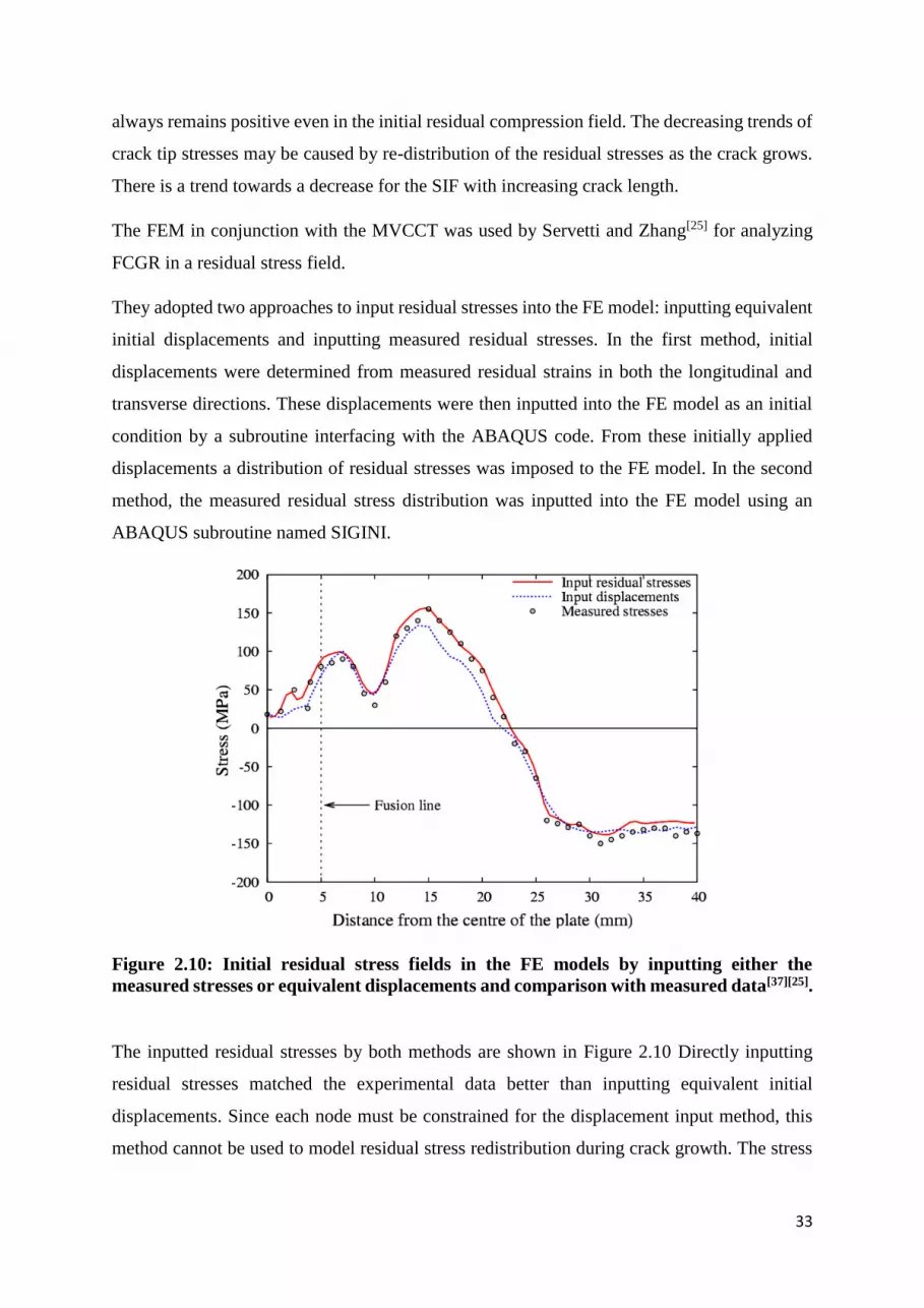
Figure 2.10: Initial residual stress fields in the FE models by inputting either the
measured stresses or equivalent displacements and comparison with measured data[37][25].
The inputted residual stresses by both methods are shown in Figure 2.10 Directly inputting
residual stresses matched the experimental data better than inputting equivalent initial
displacements. Since each node must be constrained for the displacement input method, this
method cannot be used to model residual stress redistribution during crack growth. The stress

34
input method is a better approach because the condition of the virtual work principle is satisfied
and the evolution of the residual stresses due to crack extension can be modelled.
The absolute value of Kres decreased monotonically with increasing crack length, as a
consequence of the progressive relaxation of the residual stress field due to the separation of
the body into two halves.
Recently, Liljedahl et al.[37] modelled the effect of the residual stresses on the fatigue crack
behaviour in middle tension M(T) and compact tension C(T) aluminium specimens. They used
two approaches: a crack closure approach where the effective stress intensity factor Keff was
computed, and a residual stress approach where the fatigue crack growth rate FCGR is
predicted by changes in R-ratio caused by the varying Kres. In particular, it was found that the
residual stresses accelerated the FCGR in the M(T) specimen, whereas they decelerated the
FCGR in the C(T) sample. This suggests that factors such as residual stress redistribution must
be accurately evaluated when designing damage tolerant structures based on laboratory
specimen data.
In high tensile residual stress fields, fatigue crack propagation properties are generally similar
for different applied stress ratio conditions under tensile load cycling. This similarity is due to
extremely high tensile stress ratio conditions at the crack tip which is always open during any
type of fatigue loading. Ohta et al. investigated how fatigue cracks behave differently under
highly compressive cyclic loading when they are in high tensile residual stress field[38]. They
found that fatigue crack propagation properties in tensile residual stress field under
compressive loading are similar to those under tensile loading. Only under highly compressive
cycling conditions (-100 MPa) did crack propagation rates decrease. In the experiment, fatigue
crack closure did not occur.
In summary, several researchers[21][22][23] have questioned the validity of the use of
superposition for predicting fatigue crack growth behaviour through residual stress fields.
Some criticize it because the original uncracked body residual stress is used rather than a
redistributed residual stress after crack initiation and growth. They argue that tensile residual
stress will be reduced or even eliminated by crack growth and compressive residual stress must
then also reduce to maintain equilibrium. Parker[22] disagrees, stating that the redistribution of
residual stress due to crack insertion does not invalidate the superposition principle. Other
researchers[23] have pointed out that superposition is invalid when the crack faces contact. This

35
is known to occur when a crack transitions from a compressive to a tensile residual stress
field[39].
Some researchers[40][41] accept that superposition is correct for linear elastic materials, but state
that the approach may lead to errors due to inelastic material behaviour. They argue that
residual stress can change due to plasticity at the crack tip, the insertion of a plastic wake behind
the crack tip, or due to cycle-dependent stress relaxation at the crack tip.
As summary regarding the two main methods (superposition and crack closure) for analyzing
FCGR in residual stress fields, it can be said that the first, proposed by Glinka[20] and Parker[22],
determines Reff to account for the residual stress effect, and it uses WFM or FEM for obtaining
Kres. The subsequent task is to calculate the FCGR by empirical laws. The most frequently used
are in the form of da/dN=f(ΔK,R). The Walker, Harter T-method, and NASGRO equation all
belong to this category. The second method, based on the crack closure concept originally
proposed by Elber[31][32], calculates the crack opening stress intensity factor Kopen and then the
effective stress intensity factor range ΔKeff in a combined stress field of the applied and residual
stress. For this second approach, some researchers calculate Kopen by empirical formulae[23][35],
others use FEM[42].
2.5 DIGITAL IMAGE CORRELATION IN FATIGUE CRACK
GROWTH
Photoelasticity and interferometric techniques (for example, Coherent Gradient Sensing
(CGS), Moire Interferometry, the Electronic Speckle Pattern Interferometry (ESPI), and the
Digital Speckle Photography) can measure surface deformations in real time, but they require
extensive surface preparation, for example, Moire Interferometry involves transferring of
gratings, CGS the preparation of a specularly reflective surface, and reflection photoelasticity
requires preparing birefringent coatings. In comparison the Digital Image Correlation (DIC)
method with white light illumination is a very useful tool due to the relative simplicity of the
approach[43].
In the DIC technique, random speckle patterns on a specimen surface are monitored during a
fracture event. These patterns, one before and one after deformation, are acquired, digitized,
and stored. Then, a sub-image within the undeformed image is chosen, and its location in the

36
deformed image is sought. Once the location of the sub-image in the deformed image is found,
the local displacements can be readily quantified.
One of the first applications of DIC technique to fatigue crack propagation was done by
Dawicke and Sutton[44]. They used it to analyse the critical crack tip opening angle (CTOA)
values during stable tearing of 2.3 mm thick sheets of 2024-T3 aluminum alloy.
By applying two-dimensional and three-dimensional image correlation methods, Sutton et
al.[45] carried out an investigation focused on obtaining experimental data for both the surface
strain fields and the critical CTOD in thin sheet 2024-T3 aluminum under predominantly
tensile loads. The work was then expanded to include CTOD measurements under mixed mode
loading and to the study of crack closure effects.
One method for determining when the effects of crack closure have been eliminated is to
measure the Crack Opening Displacement (COD) at positions behind the crack tip. When the
slope of the load-COD curve shows a large reduction during the loading portion of the load
cycle, the crack is assumed to be fully open and the crack tip region experiences the full effect
of the applied load. As indicated in Figure 2.11, the measured COD curves at two locations
behind the crack tip clearly show a sharp change in slope, corresponding to the elimination of
crack surface contact behind the crack tip.
Figure 2.11: CTOD vs Load for two distances behind the crack tip[45].

37
Later, Doquet and Pommier[46] used High-Resolution DIC to characterize crack propagation in
a ferritic-pearlitic steel used for railway applications and subjected to the steel to sequential
mixed-mode tests (tension-reversed torsion).
Kirugulige et al.[43] used DIC to study crack growth in edge cracked beams subjected to impact
loading. The COD was then analyzed to obtain the history of failure characterization parameter,
namely, the dynamic stress intensity factor. Figure 2.12 shows four examples of the speckle
pattern images selected from the deformed set.
Figure 2.12: Acquired speckle images of 31x31 mm2 region at various points in time
during crack formation; the current crack tip location is shown by an arrow[43].
Recently, Hamam et.al.[47] and Lopez-Crespo et.al.[48] applied the DIC technique for evaluating
the SIF in centre-cracked tension (CCT) specimens. Lopez-Crespo et.al.[49] also used DIC to
evaluate crack closure (in Al 7010 T7651 alloy) and the effect of crack-tip plasticity on stress
intensity field (in Al 2024 T351 alloy).
De Matos and Nowell[50] investigated the influence of specimen thickness on plasticity induced
closure behaviour and on fatigue crack propagation. Fatigue crack propagation in aluminium
alloy 6082 T6 was measured optically using a microscopy and a video camera with a translation
stage (Figure 2.13). Crack closure was assessed using traditional compliance techniques (clip
gauge and back face strain gauge) and DIC methods. It is thought that plasticity induced closure
has the most significant effect over the majority of the propagation life.

38
It was also found that fatigue cracks propagate faster in thick specimens rather than in thinner
specimens. This effect seems to be related to the development of different levels of crack
closure for each specimen thickness. The procedure described to measure closure using DIC is
efficient and seems to be a good alternative to conventional surface gauges, which measure
strain at a single location, often suffer damage as the crack propagates past them and are time
consuming to install.
Figure 2.13: Typical image used in Digital Image Correlation, showing pairs of points in
their original and deformed position[50].
Summarising, fatigue failure is a process of progressive fracture driven by the tensile residual
stress generated during welding. In order to analyse the fatigue strength in a welded joint is
necessary to calculate the value of K. Superposition and crack closure are the two main methods
for analyzing FCGR in residual stress fields. Superposition uses WFM or FEM for obtaining
Kres, whereas crack closure method calculates Kclos for subtracting it from ∆Kappl in order to
assess ∆Keff.
DIC is an advantageous method, in comparison to photoelasticity and/or interferometric
techniques, for measuring surface displacements in real time. The DIC technique has been
widely used for measuring the COD behind the crack tip in order to analyse the crack closure
effects.

39
CHAPTER
III
EXPERIMENTAL
METHODS

40
Chapter 3. EXPERIMENTAL METHODS
3.1 RESIDUAL STRESS MEASUREMENTS
The first stage of the project focused on the measurement of the residual stresses at surface of
the plate.
The material used was a SA508 Grade 3 Class 1 reactor pressure vessel steel, which is generally
supplied in a quenched and tempered condition. The typical mechanical properties for this kind
of steel are listed in Table 3.1.
0.2% yield strength: 448 MPa
Tensile strength: 593 MPa
Elongation: 29%
Reduction of area: 74%
Charpy energy: 138 J
Microhardness: 180-208 Hv
Table 3.1 Mechanical properties of SA508 Grade 3 Class 1 (SA508 Class 3 –ASME-) at
room temperature[51].
Before welding, the plates were stress relieved (so that any influence of machining stresses was
eliminated) by heating to 600°C for 2 h in a vacuum furnace (Francis et al.[52]). Two
180x120x20 mm3 plates were subjected to gas-tungsten arc welding (GTAW) process along
their center line. As no filler material was added during the manufacture of the plates, so the
weld was autogenous. The welding line corresponded to the long-axis centerline at the surface
of the plate (Figure 3.1).
A preheat temperature of 150°C was applied, the welding voltage was between 11.0-11.5 V
and the welding current was held constant at approximately 220 Amps. The travel speed was
75 mm/min, which resulted in the heat input being around 2 kJ/mm. The plates were not
restrained during welding.
In one of the autogenous plate samples, only a single weld pass was made. In the other, a second
identical weld pass was made in the exact same location.

41
Figure 3.1: A photograph of the plate prior to removal of a macrograph slice at location
shown for an experiment carried out by Francis et al.[53]. The welding direction was from
right to left.
The welded plates were provided in the conditions expressed above, and already cut to a
dimension of 143x120x20 mm3.
The measurement of the residual stresses was undertaken by X-Ray Diffraction in the PROTO
equipment, by using the sin2ψ method. In the experiment, the material was considered as having
a body-centered cubic (BCC) crystal structure and the measurement was oriented in the
crystallographic plane {hkl}{220}, the used X-Ray tube was Cr_Kα of wavelength 2.291 Ǻ.
In the first phase of the process the plates were analysed in the as received condition, residual
stresses were measured at the surface along the weld seam and along the adjacent HAZ in both
longitudinal and transversal directions. Later, the steel plates were ground and polished by hand
and the residual stresses were measured again at the same points, which are showed in the
Figure 3.2.
In a second phase of residual stress measurements, an end of both plates was cut by an abrasive
disk for eliminating possible effects related to redistribution/relaxation on residual stresses
and/or hardening caused by the initial cutting of the plates. The amount of material removed
during this process was 2.5 mm, then the plate thickness was subjected to a grinding and
polishing process in which another 0.5 mm of material were removed, therefore 3 mm of plate
thickness was removed in total. Unlike the first experiment, in this one the measurements were
carried out in the transversal direction to the weld seam and along thickness (Figure 3.3).

42
1 6 11 16 21mm
WELD CENTERLINE
HAZ7.5 or 8 mm
120 mm
143 mm
LONGITUDINAL (PHI=0)
TRANSVERSAL (PHI=90)
Figure 3.2: Measurement points along weld seam and HAZ for both directions:
longitudinal and transverse.
13
140
20
Dimension: mm
Measurements along
thickness every 3 mm
Measurements at surface
every 5 mm
Figure 3.3: Measurement locations in plate cut by abrasive disk. Were removed 3 mm of
material from the plate thickness: 2.5 mm by abrasive disk cutting and –afterwards- 0.5
mm by grinding and polishing processes.

43
0
0
3
6
9
12
15
18
0
-15
15
-10
10
-5
5
10
7.5
20
12.5
20
50
8
SEAM
WELD
SEAM WELD
DIMENSIONS: mm
Figure 3.4: Sample extracted from one weld plate, and electropolished showing the
measurement points (dimensions in mm).
Lastly, a 20x20x50 mm3 specimen was cut from the one run of weld plate, and a third series of
residual stress measurements was carried out on that sample (Figure 3.4). In this case, the
sample was subjected to an electropolishing process in which 85 μm of material was removed
from surface and thickness. Perchloric acid (8%) in glacial acetic acid at 50 V was used for
electropolishing.
3.2 FATIGUE TEST
Two essential requirements of the fatigue test had to be satisfied: to initiate the crack by fatigue
loading, avoiding the failure of the specimen by yielding, and to locate the crack initiation point
on the weld seam (tensile residual stress field). A standard four point Single Edge Notch Bend
(SENB4) was the specimen chosen for fulfilling these conditions (Figure 3.5).
An Excel worksheet was developed in order to design the SENB4 fatigue specimen. The main
variables to consider were the maximum load (Loadmax), beam thickness (t), stress ratio (R) and
the residual stress (σres). The specimen design was based on the Goodman diagram, and
followed the established rules by BS ISO 12108: 2002[54]. The effect of the residual stresses
was superimposed on the mean stress and the following expressions were applied in order to
relate the stress amplitude to the residual stress:

44
10
20
50
50100
SEAM WELD
AXIS OF
SYMMETRY
NOTCH
Dimensions in mmCutting of SENB4 specimen
in transversal to the weld
direction
100
50 50
50
10
20
0.5
1.0
0.5
1.0
TOP VIEW
FRONT VIEW
NOTCH
DETAILS
Figure 3.5 : Geometry of SENB4 fatigue specimen.
u
resmean
eresamp
1)( (3.1)
meanresypamp max)( (3.2)
meanamp maxmax)( (3.3)
where σe is the endurance limit, σu is the ultimate stress and σyp the yielding stress.
The values of σu and σyp were obtained from Lee and Kim[51] whereas the value of σe=360 MPa
was extracted from Fukuoka et al.[55].
In order to make sure that the element failed due to fatigue and not by yielding, it was necessary
to place the R=0.1 point in the fatigue zone (upper area between the fatigue limit and the yield
limit lines of the Goodman Diagram), however, since the fatigue limit (σe = 370 MPa) and the

45
yield limit (σyp = 450 MPa) are similar, this was not possible due to narrowness of the resulting
area; the inclusion of the residual stresses in the analysis was prevented because of the same
problem. As the design of the specimen was based on the flexure theory, the tensile zone was
superpositioned with the tensile residual stress zone generated by welding, which enhanced the
likelihood of crack initiation and propagation at the specimen surface.
The SENB4 specimens were cut by wire electrical discharge machining (EDM), and a notch
of 1 mm deep was made at the centre of the weld (zone of tensile residual stress) by the same
method in order to ensure fatigue crack initiation at this location. The EDM process was chosen
because of its little influence on the residual stress distribution of the final product since
introduces significantly lower residual stresses on the workpiece than that obtained by
conventional machining[56][57]. For the analysis of residual stress, it was important that no
redistribution or relaxation of residual stresses occurred.
Normally, in a standard fatigue test, fatigue crack growth rate (FCGR) changes due to the
variation of the applied stress intensity factor range (∆Kappl). In this case, varying residual
stresses as a consequence of crack growth means that a number of factors were changing
simultaneously. It is therefore difficult to determine the role of residual stresses on FCGR in
detail. Due to this, a non-standard tension-tension fatigue test was carried out at room
temperature on a high-cycle servo-magnetic fatigue machine (Amsler Vibrophore). During the
test, the load was decreased to keep ΔKappl constant as a function of crack length with the aim
of exactly determine the role of residual stresses on fatigue crack growth. At every 0.5 mm of
crack extension the high-frequency test was stopped for two reasons:
1) To apply a slow load cycle, allowing a series of digital images to be taken during a
complete single cycle, and
2) To decrease the applied loads in order to keep ΔKappl constant.
According to BS ISO 12108:2002[54], the applied stress intensity factor range ΔKappl for the
SENB4 specimen was calculated by means of:
∆𝐾 =𝐹
𝐵√𝑊𝑔 (
𝑎
𝑊) 101.5 (3.4)
where g(a/W) is defined as:
g(𝑎
𝑊) = 3√2𝑡𝑎𝑛𝜃 [
0.923+0.199(1−𝑠𝑖𝑛𝜃)4
𝑐𝑜𝑠𝜃] (3.5)
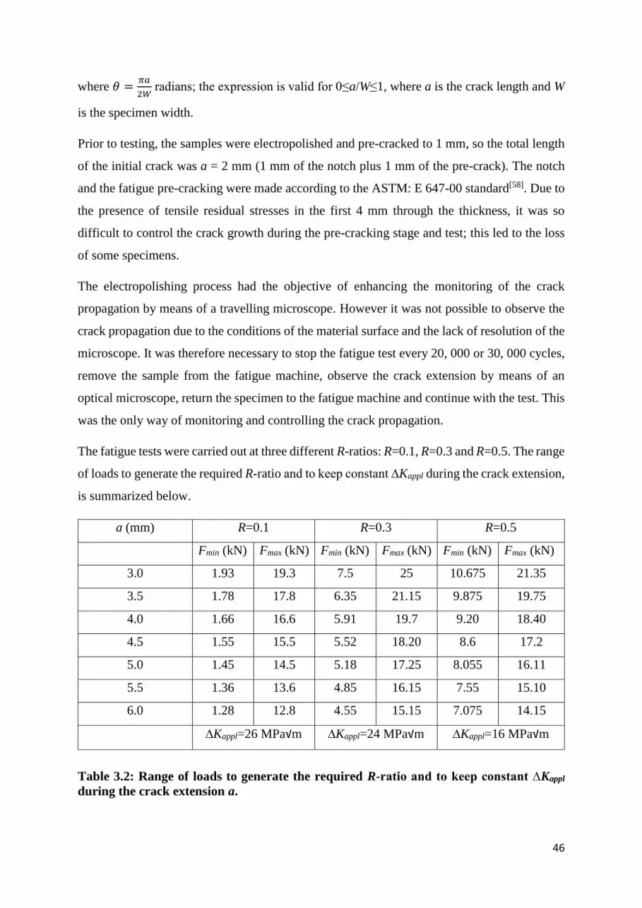
46
where 𝜃 =𝜋𝑎
2𝑊 radians; the expression is valid for 0≤a/W≤1, where a is the crack length and W
is the specimen width.
Prior to testing, the samples were electropolished and pre-cracked to 1 mm, so the total length
of the initial crack was a = 2 mm (1 mm of the notch plus 1 mm of the pre-crack). The notch
and the fatigue pre-cracking were made according to the ASTM: E 647-00 standard[58]. Due to
the presence of tensile residual stresses in the first 4 mm through the thickness, it was so
difficult to control the crack growth during the pre-cracking stage and test; this led to the loss
of some specimens.
The electropolishing process had the objective of enhancing the monitoring of the crack
propagation by means of a travelling microscope. However it was not possible to observe the
crack propagation due to the conditions of the material surface and the lack of resolution of the
microscope. It was therefore necessary to stop the fatigue test every 20, 000 or 30, 000 cycles,
remove the sample from the fatigue machine, observe the crack extension by means of an
optical microscope, return the specimen to the fatigue machine and continue with the test. This
was the only way of monitoring and controlling the crack propagation.
The fatigue tests were carried out at three different R-ratios: R=0.1, R=0.3 and R=0.5. The range
of loads to generate the required R-ratio and to keep constant ∆Kappl during the crack extension,
is summarized below.
a (mm) R=0.1 R=0.3 R=0.5
Fmin (kN) Fmax (kN) Fmin (kN) Fmax (kN) Fmin (kN) Fmax (kN)
3.0 1.93 19.3 7.5 25 10.675 21.35
3.5 1.78 17.8 6.35 21.15 9.875 19.75
4.0 1.66 16.6 5.91 19.7 9.20 18.40
4.5 1.55 15.5 5.52 18.20 8.6 17.2
5.0 1.45 14.5 5.18 17.25 8.055 16.11
5.5 1.36 13.6 4.85 16.15 7.55 15.10
6.0 1.28 12.8 4.55 15.15 7.075 14.15
∆Kappl=26 MPa√m ∆Kappl=24 MPa√m ∆Kappl=16 MPa√m
Table 3.2: Range of loads to generate the required R-ratio and to keep constant ∆Kappl
during the crack extension a.

47
The loading frequency was 100 Hz.
The relationship between the applied stress intensity factor range ∆Kappl and the crack extension
a is displayed in the Figure 3.6. The fatigue testing was carried out maintaining ∆Kappl constant
throughout all the crack propagation. The crack was propagated under the same R-ratio for a
pair of samples, the specimen with the more consistent results was taken as a basis to represent
such R-ratio in the subsequent DIC analysis. The ∆Kappl values linked to each R-ratio were:
26 MPa√m for R=0.1 (F in the Figure), 24 MPa√m for R=0.3 (B in the Figure) and 16 MPa√m
for R=0.5 (I in the Figure).
From the Figure 3.6 also it can be seen that was difficult controlling the load for keeping ∆Kappl
constant during the extension of the crack in the tensile RS zone, this generated by the
superposition of tensile loads present in the region. On the contrary, the control of the load for
the compressive zone was more straightforward.
Figure 3.6 : Constant ΔKappl during the crack propagation for each R-ratio.
∆Kappl (
MP
a√m
)
a (mm)

48
3.3 DIGITAL IMAGE CORRELATION ANALYSIS
During the fatigue test, at every 0.5 mm of crack extension the high-frequency test was stopped
and a slow load cycle was applied allowing a series of images to be taken during a single cycle.
The images were taken by means of a camera using the ISTRA 4D software by Dantec
Dynamics System, with a telephoto lens. It was necessary to use the telephoto lens because it
was not possible to set up the camera sufficiently close to the specimen, due to the position of
the Vibrophore test frame. As the analysis was in 2D, it was necessary to use a single camera.
The Q-400 system by Dantec Dynamics is an optical instrument for the full-field, non-contact
measurement of displacement and strain at a specimen surface. The system consists of two ½”
monochrome CCD cameras (1392x1040 pixels) with lenses made by Schneider Kreuznach
Germany, two high intensity LED illumination systems (HILIS) which provide a high intensity
light without heating the specimen surface and the software ISTRA 4D which controls the Q-
400 system[59][60]. The experimental setup is shown in Figure 3.7 with Figure 3.8 showing the
assembly of the SENB4 specimen in the Vibrophore machine.
Figure 3.7: Set up of the Q-400 System ISTRA 4D. The figure shows the camera with the
coupled telephoto lens (at the front), the data adquisition system, and the travelling
microscope (to the right).

49
Figure 3.8: Assembly of SENB4 specimen in the Vibrophore machine. The observation
area is the sprayed white zone at the centre of the specimen.
Several attempts to analyze the digital images obtained using the ISTRA 4D software were
made. However, due to the excessive rigid body motion, this was not possible. It was decided
to export the image files (in the HDF5 file format) to DaVis by LaVision software for analysis.
In the DaVis package, the digital images were correlated, and the displacement field in the
vicinity of the crack tip were obtained.
The observation window used for the image correlation was of 1392x1040 pixels. The cross-
correlation mode used was the integral approach, where correlation is relative to first image.
Multi-pass iteration was chosen, starting with a window size of 256x256 pixels, a weight of
1:1, and an overlap of 50% in 2 passes. The window size was decreased to 64x64 pixels, with
a weight of 1:1 and an overlap of 50% in 4 passes.
These conditions were a trade-off between the best resolution of the displacement vector field,
the minimization of the noise, and maximum allowable file size by the JMAN software.
Once had been obtained the set of displacements, these were exported as ASCII text (TXT)
files from DaVis software in to Excel. The Excel files are the only file format accepted by
JMAN software.

50
The JMAN software is a program developed at The University of Manchester based on the J-
integral method. It is based on the Finite Element theory, and written in MATLAB. The
software allows measurement of the J-integral for a crack under load from digital images taken
by the DIC technique[61][62].
Also, the set of displacements obtained by DIC were used for quantifying the Crack Tip
Opening Displacement (CTOD) by means of a code written in MATLAB. This analysis was
developed with the aim of verifying the presence of crack closure during crack extension and
for characterizing the behaviour of the crack within both tensile and compressive residual stress
fields, at different R-ratios.
Finally, the Weight Function method was implemented for deriving the residual stress intensity
factor Kres. The Weight Function for SENB4 specimen is a function that can be used to calculate
stress intensity factor arising from the residual stress field as a function of the crack tip
position[63][64]. The Weight Function was calculated by approximating the residual stress as a
constant within each of the crack growth intervals, each bounded by extensions of 0.5 mm and
varying the integral limits within the function as the crack was growing. This function was
coded in MATLAB and FORTRAN (Figure 4.11).

51
CHAPTER
IV
RESULTS
AND
DISCUSSION

52
Chapter 4. RESULTS
4.1 RESIDUAL STRESSES
The aim of this part of the study has been to characterize the residual stresses induced in a pair
of ferritic steel plates after welding, to that effect, the X-Ray Diffraction has been chosen as
the measurement technique.
4.1.1 RESIDUAL STRESSES RESULTS
The results obtained from the residual stress measurements performed to the “single weld pass”
and “2 pass weld” steel plates, at their surface along the weld seam and along the adjacent Heat
Affected Zone (HAZ), as shown in Figure 3.2, for the “as received” and “ground and polished”
conditions, are shown in Figures 4.1 (measurement in longitudinal direction) and 4.2
(measurement in transverse direction).
The charts show that in all cases the longitudinal and transverse stresses found are in
compression (except for the stresses measured along the weld seam on the plate with 2 pass
weld, in the “as received” condition in transverse direction), the stresses generated at HAZ
show higher compressive values (from -400 MPa to -500 MPa in longitudinal direction and
from -250 MPa to -500 MPa in transverse direction) than the residual stresses measured along
the weld seam.
Neither the number of runs of weld (one or two) nor the condition of the plate surface (as
received, or ground and polished) seem to have an influence on the residual stress distribution
obtained, with the exception of the aforementioned case, where the second run of weld induces
a tensile residual stress of approx. 350 MPa at the weld seam of the plate originally under
compressive residual stresses.

53
Figure 4.1: Longitudinal residual stresses measured at surface along the weldline.
Figure 4.2: Transversal residual stresses measured at surface along the weldline.
For having a more complete distribution of the residual stresses on the plates but, mainly, for
evaluating the magnitude of the transverse residual stresses present along the thickness, since
these will be the cause of the opening or the closure of the crack during the fatigue testing, a
second series of measurements was performed in the cut and ground/polished plates, in

54
transverse to the weld seam direction and along the thickness, as shown in Figure 3.3. The
results for this set of measurements are displayed in Figures 4.3 to 4.6.
Figure 4.3: Longitudinal residual stress distribution after cutting an end of the plates.
The measurement was made in transverse to the weld seam.
Figure 4.4: Transverse residual stress distribution after cutting an end of the plates. The
measurement was made in transverse to the weld seam.
1 PASS OF WELD
2 PASSES OF WELD
1 PASS OF WELD
2 PASSES OF WELD

55
Figure 4.5: Normal residual stress distribution after cutting an end of the plates. The
measurement was made through the thickness.
Figure 4.6: Transverse residual stress distribution after cutting an end of the plates. The
measurement was made through the thickness, in the transverse to weld direction.
1 PASS OF WELD
2 PASSES OF WELD
1 PASS OF WELD
2 PASSES OF WELD

56
According to Figures 4.3 to 4.6, the upper surface and the thickness of the plates are under
compression, the effect being greatest (-200 MPa to -400 MPa) at the surface and transverse
direction through the thickness. Although the measurement is made through the thickness, at
the normal direction, it also yields compression values (0 MPa to -140 MPa), these values are
low in comparison to those obtained at the surface and transverse direction through the
thickness.
The second run of weld has no influence on the residual stress distribution at the surface and
through the thickness of the plates, except for the normal direction through the thickness, in
which the second run of weld introduces tensile stresses (approx. 50 MPa), decreasing the
compression effect and approaching the stress distribution towards a residual stress free state.
The surface stress state is not a reliable indicator of the bulk stress state of an element, this
being why the electropolishing process is absolutely essential for ensuring an accurate residual
stress distribution of the sample. Bearing this in mind, a 20x20x50 mm3 specimen was
extracted from the ground and polished single weld pass plate (see Figure 3.4), and a new series
of measurements was made at the surface in the transverse to weld direction. Afterwards, the
sample was electropolished and the measurements were carried out again at the surface in the
same points and along the thickness. The results for both series of measurements are shown in
Figures 4.7 to 4.10.
From the charts (Figures 4.7 to 4.10), the high compressive effects at the surface and along the
thickness before electropolishing is observed, and the noticeable contrast with the values found
barely 85 µm below the surface and thickness after performing the electropolishing process.
Before electropolishing, and specifically at the plate surface on the weld seam, the measured
values were σres=-142 MPa for the longitudinal direction and σres=-148 MPa for the transverse
direction. After electropolishing, the measurements performed at the same points showed the
following values: σres=-6 MPa for the longitudinal direction and σres=-69 MPa for the transverse
direction.

57
Figure 4.7: Longitudinal residual stress distribution measured transverse to the weld, for
the single pass weld sample before and after electropolishing.
Figure 4.8: Transverse residual stress distribution measured transverse to the weld, in
transverse direction, for the sample before and after electropolishing.

58
Figure 4.9: Normal residual stress distribution measured through the thickness, in
normal to the weld direction, for the plate before cutting and the cut sample after
electropolishing process.
Figure 4.10: Transverse residual stress distribution measured through the thickness, in
transverse to the weld direction, for the plate before cutting and the cut sample after
electropolishing process.
When measuring the residual stresses in the longitudinal direction (Figure 4.7), the peak
compressive stresses for both conditions, before and after electropolishing, occur immediately
outside the HAZ (σres-right=-261 MPa and σres-left=-413 MPa for the sample before

59
electropolishing, and σres-right=-328 MPa and σres-left=-307 MPa for the sample after
electropolishing). For the transverse direction (Figure 4.8), the peak compressive stresses for
the sample before electropolishing are also located immediately outside the HAZ (σres-right=-
262 MPa and σres-left=-330 MPa); however, for the sample after electropolishing, this kind of
stresses arise within the HAZ (σres-right=-221 MPa and σres-left=-242 MPa).
There is no evidence of tensile stresses in the sample before electropolishing. In fact, the tensile
stresses emerge at the surface and along the thickness of the specimen after electropolishing,
showing a residual stress distribution closer to the one considered as typical for most of steels.
Regarding the measurements carried out along the thickness, the differences are also noticeable
between the residual stress distribution obtained for the specimen before and after
electropolishing.
Before electropolishing, the measured surface was under compressive stresses, these being
higher for the transverse direction with values of σres≈-270 MPa for the lower section and σres≈-
350 MPa for the upper section of the thickness (Figure 2.10). The upper section is the zone
closest to the weld seam (see Figure 3.4). The normal direction is also under compressive
residual stresses, but these stresses are lower than the abovementioned (σres≈-50 MPa for the
lower section of the thickness, reaching σres≈-140 MPa at the seam weld), as is shown in Figure
4.9. There is no evidence of tensile stresses before electropolishing.
After electropolishing, the outlook changes. Now is possible to observe the peak tensile stresses
for the normal (σres=102 MPa located at the limit of the HAZ[53]) and the transverse directions
(σres=232 MPa located on the fusion zone[53]), according to Figures 4.9 and 4.10, respectively.
The transverse direction also presents peak compressive stress (σres≈-280 MPa found at the
limit of the HAZ). Whereas for the normal direction, the peak compressive stress is rather low
(σres=-50 MPa) and occurs at the base metal far away from the weld. In general, the residual
stress values obtained for the transverse direction are higher than those obtained for the normal
direction.
Finally, it is worth mentioning that the residual stress distribution measured along the thickness,
in transverse direction (Figure 4.10), was taken as a basis for the development of the project
since this residual stress field is the one that actually originates the opening and the closing of
the crack during the tests.

60
4.1.2 RESIDUAL STRESSES DISCUSSION
For the generation and distribution of the residual stresses by welding at the plates, two
important and interrelated conditions were analysed: the number of weld passes (one or two)
and the plate surface conditions (as received, or ground and polished).
For the measurements performed along the weld, the number of passes of weld seems to have
influence only when the plate surface is in the “as received” condition. After the first pass of
weld, the plate surface undergoes high compressive stresses (σres≈-350 MPa for the
longitudinal and σres≈-300 MPa for the transverse directions, according to Figures 4.1 and 4.2);
it is tempting to try explaining this fact under the perspective of the solid-state phase
transformations that occur in ferritic steels during welding, however, such as it will be
demonstrated later, this behaviour is rather the consequence of machining and cutting effects
not completely removed during the stress relief of the plates.
The SA508 is a bainitic steel meeting two important conditions for generating compressive
residual stresses in the weld and the HAZ: a lower transformation temperature and a displacive
transformation involving both a dilatational and a shear component[53].
During the first run of weld, the thermal expansion is greater in the weld and HAZ than in the
parent metal. Generally, for most steels, when the weld cools, the parent metal withstands the
contraction in the weld and HAZ generating tensile stresses in the weld and HAZ, and
compressive stresses in the parent metal. However, the behaviour of the ferritic steels, such as
SA508 Grade 3 Class 1, do not fit in the above description. These kinds of steels undergo a
solid-state phase transformation in the weld metal and HAZ during cooling. The thermal
contraction strain is counteracted and eventually overwhelmed by the transformation strain,
leading to a pronounced reduction in tensile stresses. Even if the transformation temperature
lowers enough, there may be no scope for the accumulation of contraction stresses once the
phase transformation is completed, and the presence of compressive stresses in the weld and
HAZ is highly probable under these circumstances.
In addition, as reported by Murakawa et al.[65], preheating the plate prior to welding also has
influence on the transformation temperature, by reducing the scope for the accumulation of
thermal contraction strains after the phase transformation ceases. In this project, the plate was
preheated to a temperature of 150°C, so the phase transformation temperature during welding

61
could have been low enough to develop compressive stresses in the weld and HAZ after
cooling.
For some reason, during the second run of weld, the transformation temperature was not low
enough to counteract the contraction stresses, leading to the formation of tensile residual
stresses at the weld seam. Evidence of this is the high tensile residual stress present for the line
“as received, 2 passes of weld, measured at weld” in Figures 4.1 and 4.2, which is distinguished
due to its behaviour with respect to the rest of the lines. The transformation temperature is a
very important parameter that exerts influence on the formation of RS at weld, and in this
occasion the transformation temperature was higher than normal and could not counteract the
thermal contraction stress, leading to the mentioned result. Even the “polished, 2 passes of
weld, measured at weld” line for the same Figures also shows certain tendency towards the
tensile zone, even when the ground process induces higher compressive residual stresses at
surface.
This behaviour was also reported by Mark et al.[66] for the same kind of steel in a three-pass
weld using a low carbon steel filler wire (SD3), and they ascribed such fact to a lower level of
dilution between the filler and the base metal during the third weld pass. However, in our case,
the weld was autogenous (without the application of filler), suggesting that the presence of
tensile residual stresses along the weld after the second pass of weld, for the plate in the “as
received” condition, also could be a consequence of the annealing effect occurred during the
second run of weld. Annealing can relieve internal stresses by modifying the effective
accumulated plastic strain, as well as refine the microstructure of the weld metal[67], which
originates variations in the residual stress distribution between the different passes of weld.
The abovementioned is only applicable when the measurement is performed along the weld
and the plate is in the “as received” condition. The HAZ for this plate as well as the weld seam
and the HAZ for the “ground and polished” plate present a different behaviour in comparison
with the previously analysed weld seam at the “as received” plate, as discussed below.
In general, the residual stresses measured along the HAZ yielded higher values in compression
than those obtained for the measurement along the weld. This can easily be ascribed to the
annealing effect, which is stronger in the weld than in the HAZ. Proof of this is the decrease
(slight for the longitudinal direction and more noticeable for the transverse) of the compressive
stress values for the “as received, 2 runs of weld, at HAZ” line with respect to the “as received,
1 run of weld, at HAZ” line (see Figures 4.1 and 4.2). Although there is also the possibility that

62
the measurement points (see Figure 3.2) have not been exactly located on the intercritical HAZ
region, but rather in the boundary of the parent metal, the zone more conducive to the
development of compressive stresses due to the expansion (during welding) and the contraction
(when the weld cools) of the HAZ.
The study of both plates (single weld pass and 2 pass weld), after grinding and polishing,
showed a similar trend than that of the plates in the “as received” condition: compressive stress
values twice as high at the HAZ than at the weld. The reasons have been previously discussed.
As a general rule, the plastic deformation produced during grinding causes large compressive
stresses at the surface, whereas the generated heat leads to the formation of a slight tensile peak
just beneath it[68][69]. This is demonstrated by the results obtained from this experiment: higher
compressive values for each of the measured points at the “ground and polished” plate in
comparison with the same points measured at the plate in the “as received” condition. In other
words, the plastic deformation generated during grinding seems to be the source of the high
compressive residual stresses present at surface.
The only exceptions to the abovementioned are the measurements performed in longitudinal
direction at the weld and HAZ of the plate with single weld pass, whose values showed a stress
relaxation instead of the typical increase in compression. This may be due to the lack of control
of the grinding parameters since this process was made by hand, which might have caused
variations in the plastic deformation accumulated at surface, as well as different texture for
longitudinal and transversal directions, thereby yielding misleading results during the X-ray
diffraction measurements.
When measuring transversely to the weld seam, as shown in Fig. 3.3, the influence of grinding
effects is corroborated (see Figures 4.3 and 4.4). The second run of weld, again, seems to have
no effect on the residual stress distribution. The stress peaks located 5 mm away from the centre
of the fusion line rather suggest misleading values due to alterations on texture caused by
grinding.
From the analysis of the residual stress measurements along the thickness of the ground and
polished plates cut by abrasive disk, such cutting process and its role on the generation of
residual stresses should be addressed.
The analysis at the end (or analysis along the thickness) of the plates initially cut by abrasive
disk and later ground, showed a preferential direction for the formation of grinding residual

63
stresses (σres≈-250 MPa in the transverse direction whereas in the normal to the weld direction
the value barely was σres≈-50 MPa). It is not clear to what extent this behaviour was influenced
by the cutting process, because although 0.5 mm of material were removed by grinding after
cutting, the real scope of the stress redistribution/relaxation, the hardening and the possible
alteration of the microstructure of the material due to the heat generated in the cut-off
operation[70] was not assessed.
The phenomena of the solid-state phase transformation at the weld and HAZ continue being
debatable even when the residual stress values at such regions are in compression. The values
linked to the cutting/grinding process at the weld and HAZ regions, which spans from 0 to 6
mm (see figures 4.5 and 4.6) are σres≈-150 MPa for the normal to the weld and σres≈-350 MPa
for the transverse directions. It should be mentioned that the annealing effect, generated by the
second run of weld was rather limited, allowing the relaxation of just 50 MPa for each direction.
The large transverse stresses found in the top 6 mm of the abovementioned figures, length
which precisely matches the fusion zone, leads to think in the influence of the coarse grain and
the intergranular strains generated during the welding process. According to Fitzpatrick et
al.[71], larger grain sizes mean fewer grains contributing to the diffraction peak as well as less
accurate peak location, which in combination with the intergranular strains can yield
misleading results.
At first glance, the high compressive stresses measured by X-ray diffraction at the surface and
along the thickness before electropolishing seemed to be the consequence of the solid-state
phase transformation phenomena, however, this was misleading, as it was demonstrated by the
measurements carried out after electropolishing.
The results obtained from the analysis of the 20x20x50 mm3 sample extracted from the ground
and polished “single weld pass” plate (Figure 3.4), after electropolishing, clarified the exact
influence of the solid-state phase transformation at the weld and HAZ regions and, mainly,
revealed the strong effect of the cutting and grinding processes on the residual stress
distribution.
Although tensile residual stresses were found at subsurface in the electropolished weld and
HAZ regions, these tensile peaks do not go beyond 100 MPa in both directions and the
transverse direction shows a clear trend towards compression, which is the result of a lower
transformation temperature during welding. The presence of a tensile value out of context
(σres=300 MPa) in the longitudinal direction as well as the asymmetric and variable residual

64
stress distribution in the weld and the HAZ in both directions (Figures 4.7 and 4.8), leads to
think in misleading values due to the originated pitting during the electropolishing process.
The noticeable difference between the residual stress distribution before and after
electropolishing (Figures 4.7 to 4.10) highlights the strong influence of the grinding process on
the development of such stresses. Large compressive residual stresses at surface which
suddenly drop, approaching toward tension, just a few microns beneath the surface, is a typical
behaviour of the stresses generated during grinding[68][69].
In conclusion, the obtained residual stress distribution could be affected by:
The applied measurement technique. X-ray diffraction is not a well suited method to
the measurement of macro residual stresses because the surface stress is often an
unreliable indicator of the body as a whole[72].
The surface conditions. The surface condition represents a serious problem for the
evaluation of residual stresses by X-ray Diffraction:
if the surface is in the “as received” condition, the surface roughness essentially changes
the X-ray wave fields of the transmitted and diffracted beams inside the subsurface
regions of bulk samples, and thus influences the refractive properties of the investigated
sample area. On the other hand, the grinding process generates high compressive
residual stresses at surface which suddenly diminish barely a few microns underneath
it.
For all the abovementioned related to the unfavourable conditions of the surface, it was
highlighted the need of electropolishing the sample in order to obtain more reliable
results for the residual stress distribution in the specimen, however, the pitting
generated in the electropolished surface and the occurred residual stress relaxation
during the material removal by electropolish, can also be a source of error.
In addition, the surface may have been subjected to residual stresses not precisely
caused by welding, but rather generated by machining and grinding processes.
Although the plates were stress relieved before welding for eliminating any influence
of machining stresses, it might be possible that machining stresses were not completely
relieved.
The transformation temperature. The occurrence of solid-state phase transformation
is an undeniable fact for this kind of steel, however, the temperature at which occurs
such transformation is the key point for obtaining tensile or compressive residual stress
65
distribution. So, the transformation temperature was not low enough to completely
counteract and, even, overwhelm the thermal contraction for generating, in this way,
transverse compressive stresses in depth at the fusion zone. In reality, the reached value
by the transformation temperature just partially counteracted the thermal contraction
decreasing, to a certain extent, the magnitude of the tensile stresses occurred
transversely in depth at the fusion zone after cooling. This hypothesis is based on the
work developed by Kundu et al.[73] and on the FCGR curves generated for R=0.1, R=0.3
and R=0.5 (Figure 4.52). The FCGR curve for R=0.1 clearly exemplifies the transverse
RS distribution measured through the thickness, transverse to the weld direction (Figure
4.10): a higher crack growth rate (which coincides with the opening displayed by the
COD results) when the crack extends from a=3.0 mm to a=4.0 mm (tensile RS zone),
and a steeper decrement on FCGR (which is in agreement with the marked closure
shown by the COD results) when the crack propagates from a=5.0 mm to a=6.0 mm
(compressive RS region). Although to a lesser degree, R=0.3 and R=0.5 also agree with
the residual stress distribution aforementioned, exhibiting an increase on FCGR for the
tensile zone and a decrement on FCGR for the compressive region. This is not an
unexpected behaviour for the R-ratios since higher stress ratios (i.e. R=0.5) tend to
present limited or, even, not crack closure, while lower R-ratios (i.e. R=0.1) are more
prone to present higher levels of crack closure[74][75]. Finally, the behaviour of the R-
ratios confirmed, markedly for R=0.1 and moderately for R=0.3 and R=0.5, the presence
of tensile residual stresses for the “short” cracks (from a=3.0 mm to a=4.0 mm) and
compressive RS for the long cracks (from a=5.0 mm to a=6.0 mm).
4.1.3 RESIDUAL STRESS INTENSITY FACTOR, Kres.
In welded joint, the residual stress effect can be considered using the residual stress intensity
factor, Kres[76]. Kres is required in the prediction of FCGR[77].
In this project, the Kres values along the crack extensión was obtained by applying the Weight
Function method. The WF for SENB4 specimen is quite a simple function and it can easily be
used.

66
The Kres prediction linked to the residual stress distribution shown in Figure 4.102, is displayed
below:
Figure 4.11 Residual stress intensity factor, Kres, along the crack extension obtained by
the Weight Function method.
The results obtained by MATLAB software and FORTRAN code are very similar.
According to MATLAB software, the peak Kres value matches with the peak tensile residual
stress value (at a=3.5 mm) and the Kres curve steeply decreases as the compressive residual
stress field is reached, all this following the same trend shown by the X-ray diffraction
results.
On the other hand, the FORTRAN code predicts a peak tensile values 0.5 mm beyond than
the MATLAB does it. This is in agreement with the behaviour of the COD results which
show more opening for the same interval in where FORTRAN exhibits tensile peak values.
2 The significance of the RS distribution shown in Figure 4.10 consists in that this RS field is the one that actually originates the crack opening and crack closure during fatigue testing.
-5
0
5
10
15
20
25
0 1 2 3 4 5 6 7 8
Kre
s(M
Pa√
m)
Crack Extension "a" (mm)
VARIATION OF Kres
MATLAB
FORTRAN

67
4.2 DIGITAL IMAGE CORRELATION ANALYSIS
The obtained snapshots during the fatigue test were analysed and turned into displacement and
strain fields by means of the Digital Image Correlation software. Below (Figure 4.12) some
chosen raw images are displayed in order to show the crack behaviour under maximum load,
for the three stress-ratios R=0.1, R=0.3 and R=0.5, and for the crack growing in the three
possible scenarios: a tensile residual stress field (upper images), a residual stress free field
(middle images) and a compressive residual stress field (lower images).
At first glance, all the cracks seem to be closed, even when the tensile residual stress is
superposed to the applied load, except for the image related to the long crack when a=7.0 mm
and R=0.5 which, although –paradoxically- is growing in a compressive residual stress field
(σres=-290 MPa), evidently is totally open. So, this leads to a preliminary hypothesis which
should be corroborated by JMAN and Crack Opening Displacement (COD) methods, that the
stress-ratio R plays a preponderant role in the crack closure/opening phenomena.
Figure 4.12: Raw images showing the crack behaviour under maximum load, at different
stress-ratios and under different residual stress conditions.
10 mm
a=3.0 mm, R=0.1
TENSILE ZONE
10 mm 10 mm
10 mm 10 mm 10 mm
10 mm 10 mm 10 mm
a=3.0 mm, R=0.3
TENSILE ZONE
a=3.0 mm, R=0.5
TENSILE ZONE
a=4.5 mm, R=0.1
R.S. FREE ZONE
a=4.5 mm, R=0.3
R.S. FREE ZONE
a=4.5 mm, R=0.5
R.S. FREE ZONE
a=7.0 mm, R=0.1
COMPRESSIVE Z.
ZZONE
a=7.0 mm, R=0.3
COMPRESSIVE Z.
ZZONE
a=7.0 mm, R=0.5
COMPRESSIVE Z.
ZZONE

68
Next, from the Digital Image Correlation analysis, the maps of displacements and maximum
normal strains when the crack reaches the peak values of tension and compression of the
residual stress, for the stress ratios R=0.1, R=0.3 and R=0.5, were obtained.
First, the images corresponding to the tensile peak value σres=230 MPa (see Figure 4.10) when
the crack reaches an extension of a=3.0 mm, are displayed (Figures 4.13, 4.14 and 4.15):
Figure 4.13: Displacements and maximum normal strains for a=3.0 mm, σres=230 MPa
and R=0.1, from minimum load (upper maps) to maximum load (lower maps).

69
Figure 4.14: Displacements and maximum normal strains for a=3.0 mm, σres=230 MPa
and R=0.3, from minimum load (upper maps) to maximum load (lower maps).
Figure 4.15: Displacements and maximum normal strains for a=3.0 mm, σres=230 MPa
and R=0.5, from minimum load (upper maps) to maximum load (lower maps).

70
Figure 4.16: Displacements and maximum normal strains for a=6.0 mm, σres=-280 MPa
and R=0.1, from minimum load (upper maps) to maximum load (lower maps).
Figure 4.17: Displacements and maximum normal strains for a=6.0 mm, σres=-280 MPa
and R=0.3, from minimum load (upper maps) to maximum load (lower maps).

71
Figure 4.18: Displacements and maximum normal strains for a=6.0 mm, σres=-280 MPa
and R=0.5, from minimum load (upper maps) to maximum load (lower maps).
Above, in the Figures 4.16, 4.17 and 4.18, the images related to the compressive peak value
σres=-280 MPa when the crack extends up to a=6.0 mm are shown.
In general, the crack growth tendency is higher as R-ratio increases.
For the small crack (a=3.0 mm), the presence of a slight closure or, at least, a delay in the crack
growth for R=0.1, even when it extends in a residual stress field with a maximum tensile value
(σres=230 MPa). The crack seems to extend beyond a=3.0 mm for R=0.5 logically driven by
the high tensile residual stress field.
For the long crack (a=6.0 mm), the occurrence of closure for R=0.1 is undeniable due to the
presence of high compressive stresses (σres=-280 MPa). However, the high opening found for
R=0.3 and R=0.5 even when the crack extension is developing in a field with high compressive
stresses was unexpected.
So, in conclusion, the opening or closure of the crack is mainly controlled by the R-ratio and
not by the stress field (tensile or compressive) in which such crack is growing.

72
4.3 JMAN METHOD
Once the displacements field is obtained by means of Digital Image Correlation, the set of
values is re-arranged in EXCEL files in order to enter the data to the JMAN routine. The
obtained KJMAN are displayed in the next section.
4.3.1 JMAN RESULTS
A comparison between ∆Kappl and ∆KJMAN, for each R-ratio is shown below.
Figure 4.19: Variation of ∆Kappl and ∆KJMAN as a function of load for a=3.0 mm.
Figure 4.20: Variation of ∆Kappl and ∆KJMAN as a function of load for a=3.5 mm.
0
5
10
15
20
25
30
0 5 10 15 20 25
∆K
(M
Pa√
m)
LOAD (KN)
a=3.0, σres≈230 MPa
R=0.3, Kappl
R=0.5, Kappl
R=0.1, Kappl
0
5
10
15
20
25
30
0 5 10 15 20 25
∆K
(M
Pa√
m)
LOAD (KN)
a=3.5 mm, σres≈180 MPa
R-0.3, Kappl
R=0.5, Kappl
R=0.1, Kappl

73
Figure 4.21: Variation of ∆Kappl and ∆KJMAN as a function of load for a=4.0 mm.
Figure 4.22: Variation of ∆Kappl and ∆KJMAN as a function of load for a=4.5 mm.
0
5
10
15
20
25
30
0 5 10 15 20 25
∆K
(M
Pa√
m)
LOAD (KN)
a=4.0 mm, σres≈90 MPa
R=0.1, Kappl
R=0.3, Kappl
R=0.5, Kappl
0
5
10
15
20
25
30
0 2 4 6 8 10 12 14 16 18 20
∆K
(M
Pa√
m)
LOAD (KN)
a=4.5 mm, σres≈0 MPa
R=0.1, Kappl
R=0.3, Kappl
R=0.5, Kappl

74
Figure 4.23: Variation of ∆Kappl and ∆KJMAN as a function of load for a=5.0 mm.
Figure 4.24: Variation of ∆Kappl and ∆KJMAN as a function of load for a=5.5 mm.
0
5
10
15
20
25
30
0 2 4 6 8 10 12 14 16 18 20
∆K
(M
Pa√
m)
LOAD (KN)
a=5.0 mm, σres≈-100 MPa
R=0.1, Kappl
R=0.3, Kappl
R=0.5, Kappl
R=0.5, KJMAN
0
5
10
15
20
25
30
0 2 4 6 8 10 12 14 16 18
∆K
(M
Pa√
m)
LOAD (KN)
a=5.5 mm, σres≈-190 MPa
R=0.3, Kappl
R=0.5, Kappl
R=0.1, Kappl

75
Figure 4.25: Variation of ∆Kappl and ∆KJMAN as a function of load for a=6.0 mm.
The charts showed in Figures 4.19 to 4.25 were plotted based on the trends obtained from the
JMAN results. The JMAN results present considerable scatter, mainly at the starting and
finishing of the fatigue cycle. Due to the abovementioned, apart from the high noise level on
the results at the start of the fatigue cycle, was extremely difficult to obtain reliable information
about the crack closure by the JMAN method. It just was possible to obtain the trends which
show higher or lower values for KJMAN in relation to Kappl, depending on whether the crack
extends in the tensile or in the compressive residual stress field.
As the method is highly dependent on the chosen mask, during the analysis of the set of
displacements the plasticity zone showed by the software was avoided as far as possible. The
contour mask was changed for every load step and a pair of out of context values were
eliminated for every curve. The best trends obtained are precisely those shown in the above
figures.
From the Figures 4.19 to 4.25, it can be noticed that KJMAN curves are lined for the three R-
ratios, which indicates no occurrence of crack closure. The only clear result is the decreasing
trend of KJMAN for R=0.1 and the increasing tendency of KJMAN for R=0.3 and R=0.5 for each
one of the crack extensions analysed. This latter suggests that the crack under R=0.1 will
present less opening than that predicted for Kappl, whereas the cracks under R=0.3 and R=0.5
will display more opening than that calculated for Kappl, regardless of the residual stress field
in which the crack is propagating.
0
5
10
15
20
25
30
0 2 4 6 8 10 12 14 16
∆K
(M
Pa√
m)
LOAD (KN)
a=6.0 mm, σres≈-280 MPa
R=0.1, Kappl
R=0.3, Kappl

76
From the use of the JMAN method, two important points can be drawn:
The von Mises stress maps obtained for the first load steps present excessive noise,
which makes it impossible to establish the occurrence or not of crack closure at the start
of the fatigue cycle.
The von Mises stress results are affected by gross plasticity during the second half of
the fatigue cycle, which prevent reliable results being obtained for KJMAN.
4.3.2 JMAN DISCUSSION
The JMAN method can be divided in two stages: from the loading of the displacement sets
generated by DIC up to the generation of the von Mises stress maps, and from the analysis of
the Von Mises stress maps up to the derivation of KJMAN.
During the first phase, DIC plays an important role in the development of the JMAN method
since KJMAN depends on the correct determination of the displacement field. DIC is a non-
contact full-field method which have numerous advantages for the experimental stress/strain
analysis, however, like all methods, it also have some drawbacks such as:
1. The results of the analysis are closely related to the quality of the speckle pattern on the
specimen surface[78]. An unsuitable speckle pattern is likely to make the correlation
impossible at some facets, reducing the number of measurement points[79].
2. A calibration process should be employed to compensate for the errors associated with
the off-axis optical setup.
3. The CCD detector must remain parallel to the sample surface, since each out-of-plane
movement (translation or rotation) distorts the images[80]. If only rigid body translation
exists between the reference and deformed subsets, a single peak can be found in the
correlation coefficient distribution. In contrast, while a certain angle of relative rotation
occurs between the reference image and the deformed image, there will not be even a
single sharp peak in the correlation distribution map, and thus result in a failure in
integer pixel displacement searching[78]. To the aforementioned, we should add the out-
of-plane displacements of the specimen during loading[79].
4. Random errors affect the images acquired by the digital camera, such as excess noise
due to the CCD sensor and electromagnetic noise of the relative measurement chain[79].

77
The presence of noise and plasticity during the JMAN analysis for the three different R-ratios,
is summarised in the following table:
a R=0.1 R=0.3 R=0.5
3.0 mm Noise Low Plasticity Low Plasticity
3.5 mm Noise, Low Plasticity
4.0 mm Plasticity Plasticity
4.5 mm Noise
5.0 mm Noise Plasticity Excessive Plasticity
5.5 mm Noise Plasticity Excessive Plasticity
6.0 mm Noise, Low Plasticity Excessive Plasticity
Table 4.1: Presence of noise and plasticity beyond the crack tip.
From the table 4.1, which is based on the stresses maps observed during the JMAN analysis,
the presence of noise is evident during the fatigue cycle throughout the crack propagation for
R=0.1. Although R=0.3 and R=0.5 do not present noise, both stress ratios show plasticity, in
R=0.3 to a small degree and to a high extent for R=0.5, mainly when the crack becomes long
(it extends beyond 5 mm) and it goes into the tensile zone.
The lack of reliable KJMAN results can be explained by each of the four abovementioned DIC
points:
1. Although the speckle pattern were improved, they were not perfect and this affected the
quality of the images and, consequently, the accurate estimation of the displacements.
2. The Q-400 Istra by Dantec Dynamics was used as optical setup for taking the images,
and the calibration was carried out with this equipment, for afterwards exporting the
images to the DaVis by LaVision software in order to do the image correlation process
(because it was not possible to correct the rigid body rotation in the Q-400 Istra
software). Although there were attempts for re-calibrating the images in the DaVis
software, it was not possible to do it. This fact could also have had influence on the
KJMAN results.
3. Although attempts were made to eliminate the rigid body rotation via DaVis software,
the rotation was not eliminated totally; the out-of-plane motion is clearly visible in some
of the displacement maps generated by the software. The rigid body rotation was caused
by two facts:
The first is related to the constant placement and removal of the SENB4 specimen from
the fatigue testing machine, for verifying its crack growth in the electronic microscope.

78
A travelling microscope was used with the intention of monitoring the crack extension
but the finishing produced during electropolishing impeded such action. As a
consequence of the aforementioned, there was no certainty about the parallelism
between the CCD detector and the sample surface.
The second fact is related to the load application (ranged from 2 KN to 22 KN) which
produced flexure in the SENB4 sample and, very likely, also rotation.
4. Without a doubt, the noise effect is evident for R=0.1, due to its higher stress amplitude
in comparison with R=0.3 and/or R=0.5. The presence of noise, in combination with
the poor JMAN performance when analysing the starting of the fatigue cycle, it avoided
the detection of crack closure.
Although the noise could have come from the CCD sensor of the camera, it also could
be ascribed mainly to the vibration generated during the Vibrophore testing machine
operation.
The operating principle of the Vibrophore machine is based on the concept of a
mechanical resonator with electro-magnetic drive. The dynamic load is generated
through an oscillating system working in full resonance mode[81].
The second stage of the JMAN method (from the analysis of the stress maps up to the obtention
of KJMAN) is clearly marked by the presence of excessive plasticity remote from the crack tip,
mainly when R=0.5 and the crack becomes long (beyond 5.0 mm, see table 4.1). Since the
presence of plasticity can be attributed to the bending strains induced in the SENB4 specimen
as a result of the applied fatigue load[82], the expected behaviour was to have higher plasticity
during the first crack extensions (from a=3.0 mm to a=4.0 mm), during which the applied load
is higher, however, the behaviour was opposite: the excessive plasticity occurred at lower
loads, when the crack was beyond 5.0 mm (it should be taken into consideration that the load
was decreasing as the crack was growing, for keeping ∆K constant).
One explanation to this fact can be found by analysing the cross-section of the autogenous
weld, where the positions 5.5 mm and 6.0 mm are close to the boundary between the welded
metal and the parent metal interface, where plastic constraint may exist, such an effect may
have enhanced the presence of plasticity. Also, in this interface occurs a change in the grain
size (from coarse grain to a fine grain) and, beyond 5.0 mm, the crack extends in a compressive

79
residual stress field. The correlation between the grain size and the residual stress field with
respect to the plasticity is an issue which should be dealt with in future work.
The code JMAN is an algorithm, coded in MATLAB, used for extracting J-integral from the
displacement field obtained by DIC. A serious limitation of the method is that only elastic
conditions are considered and, hence, the area contour elements for the calculation of J must
be located in an elastically deformed region. However, materials often exhibit plastic
deformation close to the crack tip, breaking the elastic conditions. Since J is a measure of a
global strain energy release rate, a contour can be taken around the crack tip, sufficiently far
from the non-linear zone, and valid global J results are still obtained[83]. Nevertheless, in
presence of extensive plasticity, invariably the contour passes the plastic zone, generating a
path-dependent J-integral which will yield unreliable results[84]. In addition, when applying the
J-integral to the fatigue crack propagation analysis, caution should be taken when measuring
the minimum loads where the crack closure is important. Finally, with respect to the application
of the J-integral method to the analysis of stress intensity factors in residual stress fields, several
authors[85][86][87] coincide in that the approach is not convenient for such applications due to its
path-dependence in residual stress field.
The previous paragraph clearly explains the reasons of the unsatisfactory JMAN results:
presence of residual stresses and plasticity far from the crack tip, and poor performance of the
JMAN software for evaluating displacements at the starting of the fatigue cycle; unfortunately,
the latter impeded the detection of crack closure for R=0.1.
Finally, the trend of the three curves representative of R=0.1, R=0.3 and R=0.5 show
consistency with respect to the published results for similar experiments, since at high stress
ratio (R≥0.5) crack growth generally displays limited crack closure, while at low stress ratio
crack growth tends to exhibit higher levels of crack closure[74] (this was successfully
corroborated by the COD method), whereas an increase in R results in an increase in crack
propagation[88].

80
Figure 4.26: SENB4 specimen and DIC observation window where the residual stress
distribution along the crack is showed.
4.4 CRACK OPENING DISPLACEMENT METHOD
The same set of displacements obtained by the DIC technique, re-arranged in EXCEL files and
previously used by the JMAN method for obtaining KJMAN, were utilised by a MATLAB routine
for measuring the crack opening displacement (COD) at specified distances from the crack tip.
Once the displacements set was imported to the MATLAB routine, a contour map of the
horizontal displacements field (Ux) was obtained (Figure 4.27). Based on this map, a pair of
points in the wanted location were chosen. Care was taken to locate the measurement points

81
properly close to the crack path, if not (i.e. if the measurement points are placed far from the
crack path) there is the risk of analysing strains instead of displacements.
Figure 4.27: Displacements map in x-direction (Ux) showing the COD measurements
points (white rectangles) for a=4.5 mm and R=0.3. Dimensions in mm.
In this method, unlike the traditional technique that uses clip gages at the mouth of the
machined notch for inferring the COD, the opening can be directly measured at any point
behind the crack tip. For this project, all the reported COD values were measured 0.5 mm
behind the crack tip.
After inputting the value of the measurement points in the MATLAB routine, a set of COD
values for each load step during the loading fatigue cycle was plotted (Figure 4.28). The
maximum COD was extracted from the curves as is shown in Figure 4.28.
Figure 4.28: COD measurement. Each curve represents a load step. Dimensions in mm.
9
7
5
3
3 4 5 6 7 8 9 10 11 12
5 7 9 11
CR
AC
K O
PEN
ING
DIS
PLA
CEM
ENT
(mm
)
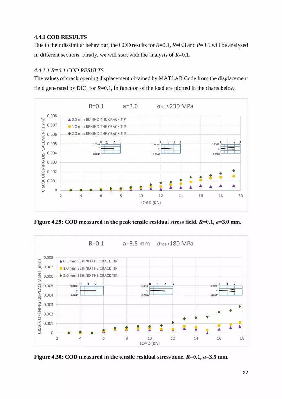
82
4.4.1 COD RESULTS
Due to their dissimilar behaviour, the COD results for R=0.1, R=0.3 and R=0.5 will be analysed
in different sections. Firstly, we will start with the analysis of R=0.1.
4.4.1.1 R=0.1 COD RESULTS
The values of crack opening displacement obtained by MATLAB Code from the displacement
field generated by DIC, for R=0.1, in function of the load are plotted in the charts below.
Figure 4.29: COD measured in the peak tensile residual stress field. R=0.1, a=3.0 mm.
Figure 4.30: COD measured in the tensile residual stress zone. R=0.1, a=3.5 mm.
0
0.001
0.002
0.003
0.004
0.005
0.006
0.007
0.008
2 4 6 8 10 12 14 16 18 20
CR
AC
K O
PEN
ING
DIS
PLA
CEM
ENT
(mm
)
LOAD (KN)
R=0.1 a=3.0 σres≈230 MPa
0.5 mm BEHIND THE CRACK TIP
1.0 mm BEHIND THE CRACK TIP
2.0 mm BEHIND THE CRACK TIP
2 1 20 3 0 3 1 2 3
0
0.0040
-0.0040
0
0.0040
-0.0040
0
0.0040
-0.0040
0
0.001
0.002
0.003
0.004
0.005
0.006
0.007
0.008
2 4 6 8 10 12 14 16 18
CR
AC
K O
PEN
ING
DIS
PLA
CEM
ENT
(mm
)
LOAD (KN)
R=0.1 a=3.5 mm σres≈180 MPa
0.5 mm BEHIND THE CRACK TIP
1.0 mm BEHIND THE CRACK TIP
2.0 mm BEHIND THE CRACK TIP
0 1 2 3 0 1 2 3 0 1 2 30.0040
0
-0.0040
0.0040
0
-0.0040
0.0040
0
-0.0040
1 0

83
Figure 4.31: COD measured in the tensile residual stress zone. R=0.1, a=4.0 mm.
In the Figures 4.29, 4.30 and 4.31 can be seen the COD values as the load increases during the
loading fatigue cycle, while the crack extends in a tensile residual stress field. In this analysis,
the cracks extending from a=3.0 mm to a=4.0 mm will be considered as “short cracks”. Also,
a sketch of the crack for minimum, medium and maximum load, as the crack is growing, is
included.
Even when the crack is growing in a tensile RS field, it can be noticed the presence of crack
closure, mainly for the shortest crack a=3.0 mm (Figure 4.29), it which remains totally closed
during the first half of the fatigue cycle, after this the crack gradually starts to open, but this
opening starts 1 mm beyond the crack tip since the rest of the crack (from the tip up to 0.5 mm
behind the tip) remains closed during the whole cycle, such as is shown in the crack sketches.
It should be noted that this crack extends in the peak tensile residual stress field (σres=230 MPa).
Although the tensile residual stress field decreases for the rest of the short cracks (a=3.5 mm
and a=4.0 mm) shown in the Figures 4.30 and 4.31, the crack closure does not increase but
rather it is maintained. Both cracks also remain closed during the first half of the fatigue cycle,
similar to the shortest crack a=3.0 mm but, unlike this, the crack mouth opens more for a=3.5
mm and, in general, a=4.0 mm exhibits more opening than the rest of the “short” cracks. The
crack continues being closed up to 0.5 mm behind the tip during the whole cycle.
0
0.001
0.002
0.003
0.004
0.005
0.006
0.007
0.008
2 4 6 8 10 12 14 16 18
CR
AC
K O
PEN
ING
DIS
PLA
CEM
ENT
(mm
)
LOAD (KN)
R=0.1 a=4.0 mm σres≈90 MPa
0.5 mm BEHIND THE CRACK TIP
1.0 mm BEHIND THE CRACK TIP
2.0 mm BEHIND THE CRACK TIP
3.0 mm BEHIND THE CRACK TIP
0 1 2 3 0 1 2 30.0040
0
-0.0040
0.0040
0
-0.0040
0.0040
0
-0.0040
0 1 2 3

84
Figure 4.32: COD measured in a residual stress free zone. R=0.1, a=4.5 mm.
a=4.5 mm (Figure 4.32) is considered as a crack extending in a residual stress free zone and,
similar to the previously mentioned “short” cracks, it presents closure during the first half of
the fatigue cycle but opening for the rest of it. However the crack is not fully open, it remains
closed from the tip up to 1.0 mm behind of it, but open for the rest of the crack path.
Figure 4.33: COD measured in the compressive residual stress zone. R=0.1, a=5.0 mm.
0
0.001
0.002
0.003
0.004
0.005
0.006
0.007
0.008
2 4 6 8 10 12 14 16
CR
AC
K O
PEN
ING
DIS
PLA
CEM
ENT
(mm
)
LOAD (KN)
R=0.1 a=4.5 mm σres≈0 MPa
0.5 mm BEHIND THE CRACK TIP
1.0 mm BEHIND THE CRACK TIP
2.0 mm BEHIND THE CRACK TIP
3.0 mm BEHIND THE CRACK TIP
0 1 2 3 0 1 2 3 0 1 2 30.0040
0
-0.0040
0.0040
0
-0.0040
0.0040
0
-0.0040
0
0.001
0.002
0.003
0.004
0.005
0.006
0.007
0.008
2 4 6 8 10 12 14 16
CR
AC
K O
PEN
ING
DIS
PLA
CEM
ENT
(mm
)
LOAD (KN)
R=0.1 a=5.0 mm σres≈-100 MPa
0.5 mm BEHIND THE CRACK TIP
1.0 mm BEHIND THE CRACK TIP
2.0 mm BEHIND THE CRACK TIP
3.0 mm BEHIND THE CRACK TIP
0 1 2 3 0 1 2 30.0040
0
-0.0040
0.0040
0
-0.0040
0.0040
0
-0.0040
0 1 2 3

85
Figure 4.34: COD measured in the compressive residual stress zone. R=0.1, a=5.5 mm.
Figure 4.35: COD measured in the peak compressive RS field. R=0.1, a=6.0 mm.
Regarding the long cracks (these being considered from a=5.0 mm to a=6.0 mm) shown in the
Figures 4.33, 4.34 and 4.35, which grow in a compressive residual stress field; the crack
behaviour can be related to the residual stress field in which they are developing.
Starting with the analysis of a=5.0 mm (Figure 4.33), which is propagating in a compressive
residual stress field σres=-100 MPa, it can be seen that the crack remains closed during two
0
0.001
0.002
0.003
0.004
0.005
0.006
0.007
0.008
2 4 6 8 10 12 14
CR
AC
K O
PEN
ING
DIS
PLA
CEM
ENT
(mm
)
LOAD (KN)
R=0.1 a=5.5 mm σres≈-190 MPa
0.5 mm BEHIND THE CRACK TIP
1.0 mm BEHIND THE CRACK TIP
2.0 mm BEHIND THE CRACK TIP
3.0 mm BEHIND THE CRACK TIP
0 1 2 3 0 1 2 30.0040
0
-0.0040
0.0040
0
-0.0040
0.0040
0
-0.0040
0
0.001
0.002
0.003
0.004
0.005
0.006
0.007
0.008
2 4 6 8 10 12 14
CR
AC
K O
PEN
ING
DIS
PLA
CEM
ENT
(mm
)
LOAD (KN)
R=0.1 a=6.0 mm σres≈-280 MPa
0.5 mm BEHIND THE CRACK TIP
1.0 mm BEHIND THE CRACK TIP
2.0 mm BEHIND THE CRACK TIP
3.0 mm BEHIND THE CRACK TIP
0 1 2 3 0 1 2 3 0 1 2 30.0040
0
-0.0040
0.0040
0
-0.0040
0.0040
0
-0.0040
0 1 2 3

86
thirds of the cycle and the opening, which happens in the remaining third, it begins 2.0 mm
behind the crack tip. The behaviour of a=5.5 mm and a=6.0 mm is according with the increment
of compressive residual stresses in the region exhibiting total crack closure during the whole
fatigue cycle. a=5.5 mm (Figure 4.34) gives a weak evidence of opening at the crack mouth at
maximum load, but this “opening” is so negligible that the crack can be considered as fully
closed during all the cycle. The crack closure is much more evident for a=6.0 mm (Figure 4.35)
since this crack is growing in a peak compressive residual stress field (σres=-280 MPa).
When comparing the opening levels of the set of short cracks growing in the tensile zone
against the long cracks developing in the compressive zone, it is reasonable to observe that
short cracks open much more than long cracks.
4.4.1.2 R=0.3 AND R=0.5 COD RESULTS
The results of COD versus applied load are plotted. Both R-ratios are analysed together due to
the similarity in their behaviour.
From the Figures 4.36 to 4.43, it can be observed that the influence of compressive residual
stresses is negligible on R=0.3 and R=0.5: the crack opens independently of the existence of
compressive residual stresses in the element.
According to Figures 4.36 and 4.37, at the start of the propagation (a=3.0 mm) the crack
behaviour for R=0.3 and R=0.5 is almost exactly the same, just a very slight closure in the first
load step occurs for R=0.3 (Figure 4.36); as the crack continues growing, there is greater
opening for R=0.5 in comparison with R=0.3 (see Figures 4.38 to 4.43). There is a noticeable
difference in the opening levels between both R-ratios when the crack reaches 6.0 mm of
extension (Figures 4.42 and 4.43). For the long cracks a=6.0 mm with R=0.3 and R=0.5,
extending in a high compressive residual stress field, there is no opening rise during the first
pair of load steps at the start of the fatigue cycle (Figure 4.43).

87
Figure 4.36 COD measured in the peak tensile residual stress field. R=0.3, a=3.0 mm.
Figure 4.37: COD measured in the peak tensile residual stress field. R=0.5, a=3.0 mm.
0
0.001
0.002
0.003
0.004
0.005
0.006
0.007
0.008
7 9 11 13 15 17 19 21 23
CR
AC
K O
PEN
ING
DIS
PLA
CEM
ENT
(mm
)
LOAD (KN)
R=0.3 a=3.0 mm σres≈230 MPa
0.5 mm BEHIND THE CRACK TIP
0 1 2 3 0 1 2 3 0 1 2 30.0040
0
-0.0040
0.0040
0
-0.0040
0.0040
0
-0.0040
0
0.001
0.002
0.003
0.004
0.005
0.006
0.007
0.008
10 12 14 16 18 20 22
CR
AC
K O
PEN
ING
DIS
PLA
CEM
ENT
(mm
)
LOAD (KN)
R=0.5 a=3.0 σres≈230 MPa
0.5 mm BEHIND THE CRACK TIP
0 1 2 3 0 1 2 3 0 1 2 30.0040
0
-0.0040
0.0040
0
-0.0040
0.0040
0
-0.0040

88
Figure 4.38: COD measured in the tensile residual stress zone. R=0.3, a=4.0 mm.
Figure 4.39: COD measured in the tensile residual stress zone. R=0.5, a=4.0 mm.
0
0.001
0.002
0.003
0.004
0.005
0.006
0.007
0.008
6 8 10 12 14 16 18 20
CR
AC
K O
PEN
ING
DIS
PLA
CEM
ENT
(mm
)
LOAD (KN)
R=0.3 a=4.0 mm σres≈90 MPa
0.5 mm BEHIND CRACK TIP
1.0 mm BEHIND CRACK TIP
0 1 2 3 0 1 2 3 0 1 2 30.0040
0
-0.0040
0.0040
0
-0.0040
0.0040
0
-0.0040
0
0.001
0.002
0.003
0.004
0.005
0.006
0.007
0.008
10 11 12 13 14 15 16 17 18 19
CR
AC
K O
PEN
ING
DIS
PLA
CEM
ENT
(mm
)
LOAD (KN)
R=0.5 a=4.0 mm σres≈90 MPa
0.5 mm BEHIND THE CRACK TIP
1.0 mm BEHIND THE CRACK TIP
0 1 2 3 0 1 2 3 0 1 2 30.0040
0
-0.0040
0.0040
0
-0.0040
0.0040
0
-0.0040

89
Figure 4.40: COD measured in the compressive residual stress zone. R=0.3, a=5.0 mm.
Figure 4.41: COD measured in the compressive residual stress zone. R=0.5, a=5.0 mm.
0
0.001
0.002
0.003
0.004
0.005
0.006
0.007
0.008
6 8 10 12 14 16 18
CR
AC
K O
PEN
ING
DIS
PLA
CEM
ENT
(mm
)
LOAD (KN)
R=0.3 a=5.0 mm σres≈-100 MPa
0.5 mm BEHIND THE CRACK TIP
1.0 mm BEHIND THE CRACK TIP
2.0 mm BEHIND THE CRACK TIP
0 1 2 3 0 1 2 3
0 1 2 3
0.0040
0
-0.0040
0.0040
0
-0.0040
0.0040
0
-0.0040
0
0.001
0.002
0.003
0.004
0.005
0.006
0.007
0.008
8 9 10 11 12 13 14 15 16 17
CR
AC
K O
PEN
ING
DIS
PLA
CEM
ENT
(mm
)
LOAD (KN)
R=0.5 a=5.0 mm σres≈-100 MPa
0.5 mm BEHIND THE CRACK TIP
1.0 mm BEHIND THE CRACK TIP
2.0 mm BEHIND THE CRACK TIP0 1 2 3
0 1 2 3 0 1 2 3
0.0040
0
-0.0040
0.0040
0
-0.0040
0.0040
0
-0.0040

90
Figure 4.42: COD measured in the peak compressive RS field. R=0.3, a=6.0 mm.
Figure 4.43: COD measured in the peak compressive RS field. R=0.5, a=6.0 mm.
0
0.001
0.002
0.003
0.004
0.005
0.006
0.007
0.008
4 6 8 10 12 14 16
CR
AC
K O
PEN
ING
DIS
PLA
CEM
ENT
(mm
)
LOAD (KN)
R=0.3 a=6.0 mm σres≈-280 MPa
0.5 mm BEHIND THE CRACK TIP
1.0 mm BEHIND THE CRACK TIP
2.0 mm BEHIND THE CRACK TIP
3.0 mm BEHIND THE CRACK TIP
0 1 2 3
0 1 2 3 0 1 2 3
0.0040
0
-0.0040
0.0040
0
-0.0040
0.0040
0
-0.0040
0
0.001
0.002
0.003
0.004
0.005
0.006
0.007
0.008
6 7 8 9 10 11 12 13 14 15
CR
AC
K O
PEN
ING
DIS
PLA
CEM
ENT
(mm
)
LOAD (KN)
R=0.5 a=6.0 mm σres≈-280 MPa
0.5 mm BEHIND THE CRACK TIP
1.0 mm BEHIND THE CRACK TIP
2.0 mm BEHIND THE CRACK TIP
3.0 mm BEHIND THE CRACK TIP
0 1 2 3
0 1 2 3 0 1 2 3
0.0040
0
-0.0040 0.0040
0
-0.0040
0.0040
0
-0.0040

91
4.4.1.3 COD FROM a=3.0 mm TO a=6.0 mm FOR R=0.1, R=0.3 AND R=0.5.
Next, the COD values obtained for each crack extension for R=0.1, R=0.3 and R=0.5, and
measured at selected positions behind the crack tip, along its wake, are displayed. Since the
crack propagation under the influence of R=0.1 is the most affected by the residual stress field
and its opening/closure presents more complexity, it will be analysed for three different
positions behind the crack tip and in a smaller range for COD.
Figure 4.44: COD measured 0.5 mm behind the crack tip, along the total crack
propagation, for R=0.1.
According to the Figures from 4.29 to 4.35, and considering as opened cracks only those with
COD>0.001 mm, it can be observed that the long cracks (a=5.0 mm to a=6.0 mm) remain fully
closed during their extension on the compressive residual stress field. The “short” cracks (a=3.0
mm to a=4.0 mm), which grow in the tensile residual stress field, invariably remain closed up
to 0.5 mm behind the crack tip during the whole fatigue cycle (see Figure 4.44). The opening
of these cracks is a slow process and occurs when the fatigue cycle is finishing, this when the
COD measurement is carried out 1.0 mm behind the crack tip (see Figure 4.45). For the
measurement carried out 2.0 mm behind the crack tip, it can be seen that the opening of the
crack is faster and it happens after having passed the half of the loading fatigue cycle (see
Figure 4.46).
0
0.0005
0.001
0.0015
0.002
0 2 4 6 8 10 12 14 16 18
CR
AC
K O
PEN
ING
DIS
PLA
CEM
ENT
(mm
)
LOAD (kN)
R=0.1, 0.5 mm BCT
a=3.0 mm
a=3.5 mm
a=4.0 mm
a=4.5 mm
a=5.0 mm
a=5.5 mm
a=6.0 mm

92
In general, R=0.1 shows just a very slight opening (Figure 4.46) in comparison with R=0.3
(Figure 4.47) or, even more, contrasting it vs R=0.5 (Figure 4.48). R=0.1 is the only stress ratio
which is affected by the residual stress field, generating total closure for the long cracks (a=5.0
mm to a=6.0 mm) growing in the compressive RS field during all the fatigue cycle. The
opening level present in the short cracks (a=3.0 mm to a=4.0 mm) which propagate in the
tensile RS field is very low too.
Figure 4.45: COD measured 1.0 mm behind the crack tip, along the total crack
propagation, for R=0.1.
Figure 4.46: COD measured 2.0 mm behind the crack tip, along the total crack
propagation, for R=0.1.
0
0.0005
0.001
0.0015
0.002
0 2 4 6 8 10 12 14 16 18
CR
AC
K O
PEN
ING
DIS
PLA
CEM
ENT
(mm
)
LOAD (kN)
R=0.1, 1.0 mm BCT
a=3.0 mm
a=3.5 mm
a=4.0 mm
a=4.5 mm
a=5.0 mm
a=5.5 mm
a=6.0 mm
0
0.0005
0.001
0.0015
0.002
0.0025
0 2 4 6 8 10 12 14 16 18
CR
AC
K O
PEN
ING
DIS
PLA
CEM
ENT
(mm
)
LOAD (kN)
R=0.1, 2.0 mm BCT
a=3.0 mm
a=3.5 mm
a=4.0 mm
a=4.5 mm
a=5.0 mm
a=5.5 mm
a=6.0 mm

93
Figure 4.47: COD measured 0.5 mm behind the crack tip, along the total crack
propagation, for R=0.3.
Figure 4.48: COD measured 0.5 mm behind the crack tip, along the total crack
propagation, for R=0.5.
The stress ratios R=0.3 (Figure 4.47) and R=0.5 (Figure 4.48) show similar behaviour:
significant opening with a weak evidence of crack closure.
0
0.001
0.002
0.003
0.004
0.005
0.006
4 6 8 10 12 14 16 18
CR
AC
K O
PEN
ING
DIS
PLA
CEM
ENT
(mm
)
LOAD (kN)
R=0.3
a=3.0 mm
a=3.5 mm
a=4.0 mm
a=4.5 mm
a=5.0 mm
a=5.5 mm
a=6.0 mm
0
0.001
0.002
0.003
0.004
0.005
0.006
6 8 10 12 14 16 18
CR
AC
K O
PEN
ING
DIS
PLA
CEM
ENT
(mm
)
LOAD (kN)
R=0.5
a=3.0 mm
a=3.5 mm
a=4.0 mm
a=4.5 mm
a=5.0 mm
a=5.5 mm
a=6.0 mm

94
The residual stress field does not seem to have influence on R=0.3 and R=0.5: the crack opens
independently of the existence of compressive residual stresses in the ligament.
In fact, as R increases, the crack driving force also increases and, thus, the crack opening
displacement rises as well. Also, at high R-ratios (i.e. R=0.5), the long cracks grow faster than
short cracks, even when long cracks are growing in a compressive RS field while short cracks
grow in a tensile RS field.
4.4.1.4 ∆Keff AND FCGR.
Taking data from the Figures 4.29 to 4.43 the load at which the crack starts to open, the
“CLOSURE LOADS” chart was plotted (Figure 4.49).
Figure 4.49: Closure loads extracted from the COD results.
With this Figure as a base, the closure loads were linked to their inherent K (calculated by the
BS ISO 12108:2002, equation 3.4) during the crack propagation. The stress intensity factor this
way obtained was denominated Kclos, and is displayed in the Figure 4.50.
The Figures 4.49 and 4.50 exhibit the same trend for the three R-ratios: Kclos increases as the
crack leaves the tensile RS region behind and goes into the compressive RS zone, this for
R=0.1, whereas for R=0.3 and R=0.5 Kclos takes the value of 0 MPa√m during almost all the
0
2
4
6
8
10
12
14
2.5 3 3.5 4 4.5 5 5.5 6 6.5
LOA
D (
KN
)
CRACK LENGTH (mm)
CLOSURE LOADS
R=0.1
R=0.3
R=0.5

95
crack extension and only slightly increases its value between 3.38 MPa√m and 5.5 MPa√m
when the crack reaches the peak compressive residual stress value.
Figure 4.50: Kclos for R=0.1, R=0.3 and R=0.5.
Figure 4.51: ∆Keff for R=0.1, R=0.3 and R=0.5.
0
5
10
15
20
25
30
2.5 3 3.5 4 4.5 5 5.5 6 6.5
Kcl
os
(MP
a√m
)
CRACK LENGTH (mm)
Kclosure
R=0.1
R=0.3
R=0.5
0
5
10
15
20
25
30
2.5 3 3.5 4 4.5 5 5.5 6 6.5
∆K
eff
(MP
a√m
)
CRACK LENGTH (mm)
∆Keff
R=0.1
R=0.3
R=0.5 ∆Kappl(R=0.
3)
∆Kappl(R=0.
5)

96
The effective stress intensity factor range ∆Keff for every crack extension was calculated by
subtracting the Kclos value from ∆Kappl values. The results are summarised in the Figure 4.51.
In this Figure it can be seen that, for R=0.1, ∆Keff decreases as the crack becomes longer and
grows into the compressive residual stress field, making evident the presence of crack closure
such as had previously been demonstrated by the COD results. The analysis for R=0.3 and
R=0.5 indicates the non-presence of crack closure since ∆Keff=∆Kappl, the only exception is
when the crack reaches the peak compressive RS value (a=6.0 mm) it which generates a slight
decrement in the ∆Keff value.
In the ∆Keff chart of the Figure 4.51, the ∆Kappl line for every R-ratio is included for a better
understanding of the closure/opening effects and their interrelation with the R-ratio and the
residual stress field.
Figure 4.52: FCGR for R=0.1, R=0.3 and R=0.5.
Finally, the fatigue crack growth rate (FCGR) was also assessed. The Figure 4.52 shows the
variation on FCGR as the crack was growing in a RS field changing from tension to
compression, for each one of the three R-ratios. In the chart can be observed as the low R (R=0.1
in this case) is more affected by the residual stress field than higher R (i.e. R=0.3 or R=0.5).
R=0.1 displays a higher FCGR for the tensile zone and a steeper decrement on the FCGR for
the compressive region in comparison with R=0.3 and R=0.5, it which shows the high closure
1.00E-07
1.00E-06
1.00E-05
1.00E-04
1.00E-03
2.5 3 3.5 4 4.5 5 5.5 6 6.5
da/
dN
(m
m/c
ycle
)
CRACK LENGTH (mm)
FATIGUE CRACK GROWTH RATE
R=0.1
R=0.3
R=0.5

97
levels for the compressive zone of R=0.1. By contrast, R=0.3 and R=0.5 are not greatly affected
by the change in RS field, just a slight decrement in FCGR when the long cracks go into the
compressive RS zone. It is worth mentioning that the behaviour of R=0.3 and R=0.5 is very
similar and almost linear since the fatigue testing was carried out under constant ∆Kappl.
4.4.2 COD DISCUSSION
The FCGR behaviour for R=0.1 markedly differs from R=0.3 and R=0.5: R=0.1 shows hardly
any opening when the crack grows in the tensile residual stress zone, and total closure when
the crack develops in the compressive RS zone, whereas R=0.3 and R=0.5 do not show
evidence of crack closure (except when the crack reaches a=6.0 mm), just an increasing
opening which is steeper for R=0.5.
The differences in FCGR behaviour for the abovementioned R-ratios can be the consequence
of the influence of the mean stresses, generated by the tensile fatigue loads, on the crack closure
phenomena inherent to the crack propagation. Grain size may also be an important factor which
will be addressed in this discussion.
4.4.2.1 R=0.1
Firstly, analysing R=0.1 for the crack extending from a=3.0 mm to a=4.0 mm (Figures 4.29 to
4.31), it can be observed the presence of crack closure even when the crack extends in a tensile
RS field. This finding is not surprisingly since the closure can have its origin in, at least, three
sources: a) during crack growth, material is plastically strained at the crack tip, and due to the
restraint of surrounding elastic material on this residual stretch, some closure at the crack
surfaces occurs at positive loads (plasticity-induced crack closure)[89], b) during cyclic crack
growth, contact shielding arises from the wedging action of fracture surface asperities
(roughness-induced fatigue crack closure)[90], and c) during welding, the transformation from
an austenitic to martensitic phase, which occurs locally in the region around the crack tip,
involves a positive volume change, the constraint of surrounding untransformed material will
place such regions under compression (phase-transformation-induced crack closure)[90].
The cracks a=3.0 mm, a=3.5 mm and a=4.0 mm are affected by the two kinds of closure:
plasticity-induced crack closure, due to the compressive residual stress developed in the plastic
wake during the crack propagation, and roughness-induced crack closure, since the contact
shielding is promoted by low load ratios (R=0.1, in this case) and by coarse-grained
materials[90], and the cracks are extending in the weld metal which presents as a characteristic
the coarsening of its microstructure.

98
In other ways, the crack extensions a=5.0 mm, a=5.5 mm and a=6.0 mm develop in a
compressive residual stress field generated as a consequence of the welding process. The
aforementioned cracks are also influenced by at least two kinds of closure: plasticity-induced
crack closure and roughness-induced crack closure due only to low ratio, since the crack no
longer develops in the coarse-grained zone, but rather in a grain-refined region.
By comparing the set of cracks developing in the tensile RS field (Figures 4.29 to 4.31) vs the
cracks growing in the compressive zone (Figures 4.33 to 4.35), one can observe that, in general,
the results are the expected: opening (at least in minimum extent) for the cracks growing in the
tensile RS field and total closure for those extending in the compressive region. The closure
takes the half of the loading fatigue cycle when the cracks extend in the tensile region, such as
is shown in the COD results.
Although more opening was expected for a=3.0 mm compared with a=3.5 mm and/or a=4.0
mm, since the X-ray diffraction analysis carried out to the uncracked sample demonstrated that
the tensile residual stress peak σres=230 MPa was located in a=3.0 mm, this did not happen; the
three measured positions (a=3.0 mm, a=3.5 mm and a=4.0 mm) presented the same closure
levels. This fact may be explained from the perspective of the stress redistribution: the growth
of the crack redistributed the original tensile residual stress spreading it near the tip
region[91][92].
Although the main “driving force” for generating crack propagation in the tensile region is the
tensile residual stress, the grain size effect on fatigue crack growth may be important. Grain
size affect the crack path and the FCGR locally, when the crack propagates from coarser to a
finer grain region, as the distribution generated at weld and at the HAZ, respectively, as a
consequence of the welding processes in ferritic steels, the interface between coarser and finer
grain (in our case located approximately at the HAZ, where the residual stress changes from
tension to compression) may behaves as a grain boundary barrier restricting the crack
propagation[93][94].
When a fatigue crack is propagating through a residual stress field in welded plate, the effective
stress intensity factor at the crack tip is the sum of the stress intensity factor due to residual
stress and the stress intensity factor due to external loading[95]. In the case of the cracks a=5.0
mm, a=5.5 mm and a=6.0 mm, as the fatigue test was tension-tension, the stress intensity factor
associated with the external loading is tensile too, whereas the local residual stress is highly
compressive. As the intensity factor related to external loading (tension) is not able to overcome

99
the intensity factor associated to the local residual stress (compression), the set of cracks
develops total closure (see Figures 4.33, 4.34 and 4.35).
4.4.2.2 R=0.3 AND R=0.5
The analysis for R=0.3 and R=0.5 almost exclusively shows crack opening (Figures from 4.36
to 4.43), even when the crack reaches and goes into the region of high compressive residual
stress. The only exception is when the crack reaches the peak compressive RS value (a=6.0
mm, σres=-280 MPa) and a slight closure is observed at the start of the fatigue cycle. One way
for understanding the behaviour of such stress ratios is to remember the theoretical bases of the
crack extension and its relationship regarding plasticity.
The crack advancement is governed by irreversible plastic flow. The slip irreversibilities
introduced during forward fatigue loading is not recovered fully during reverse loading, which
generates the crack propagation[96]. The great amount of plasticity occurring at and ahead the
crack tip promotes a large degree of slip irreversibilities, which increases with increasing crack
size[97]. So, according with the aforementioned, higher FCGR result from the excessive
plasticity ahead of the fatigue crack tip[98]. It is worth mentioning that, based on the results
yielded by JMAN method, the plasticity was excessive ahead the crack tip during the crack
driving force analysis for R=0.3 and R=0.5, it which can be an indicative of accelerated crack
growth.
However, the parameter that could have a stronger influence on the steeper FCGR is linked
with the mean stress. Although a mean stress itself cannot cause fatigue failure, it has a
considerable impact on the fatigue behaviour. The mean stress is often, especially in association
with crack propagation, characterised by R-ratio[99]. Superposition of a static compressive
residual stress and a cyclic tensile applied stress can have two outcomes, crack opening or crack
closure, depending on whether crack closure is overcome or not[100]. In the case of the set of
cracks extending in the compressive region for R=0.1, the stress ratio R was not able to
overcome the compressive residual stress effects, resulting in crack closure during the whole
fatigue cycle. On the other hand, when analysing the same set of cracks (a=5.0 mm to a=6.0
mm) but now for R=0.3 and R=0.5, the compressive residual stress effects (closure) are
immediately overcome by the tensile applied stresses, resulting in crack opening and higher
FCGR. It should be noted that an increase in R results in an increase in FCGR.
100
CHAPTER
V
CONCLUSIONS
101
Chapter 5. CONCLUSIONS
5.1 CONCLUSIONS
In this thesis a test-piece was developed having a residual stress field that varied from tension
to compression through a region of weld metal in a SA508 Grade 3 Class 1 ferritic steel. During
the fatigue test, ∆Kappl was kept constant to accurately determine the role of the residual stresses
on the fatigue crack growth for a range of R-ratios. The Digital Image Correlation technique
was used to obtain the surface displacements around the crack tip from the fatigue test, and
later these displacements were analysed by the JMAN method using a MATLAB code to obtain
KJMAN. DIC was an excellent technique for measuring both stress intensity factor and COD as
means of characterising the crack driving force.
From the project, the following conclusions can be drawn:
The obtained residual stress distribution was more affected by the sample surface
conditions than by the welding process. The solid-state phase transformation
temperature was not low enough to overwhelm the thermal contraction and just partially
counteracted it, generating a decrease in the magnitude of the tensile stresses existing
transversely in depth at the fusion zone after cooling.
In particular, the unsatisfactory JMAN results are ascribed to the presence of residual
stresses and gross plasticity in the zone of analysis, as well as the lack of detection of
crack closure is due to the poor performance of the JMAN software for evaluating
displacements at the starting of the fatigue cycle.
In general, the trend of the JMAN results agrees with the COD results and with
published results for similar experiments: as R increases, FCGR also increases.
The FCGR behaviour for R=0.1 markedly differs from R=0.3 and R=0.5: R=0.1 shows
hardly any opening when the crack grows in the tensile residual stress zone, and total
closure when the crack develops in the compressive RS zone, whereas R=0.3 and R=0.5
do not show evidence of crack closure (except when the crack reaches a=6.0 mm), just
an increasing opening which is steeper for R=0.5. The differences in FCGR behaviour
for the abovementioned R-ratios can be the consequence of the influence of the mean
stresses.

102
The accelerated FCGR for R=0.3 and R=0.5 is due to the great amount of plasticity at
and ahead the crack tip which promotes a large degree of slip irreversibilities, which
increases as the crack size increases too.
FCGR is influenced to a greater degree by the stress ratio R and in a lesser extent by
the residual stress field.
The residual stress field exerts a greater influence at lower R-ratios (i.e. R=0.1) than at
higher R-ratios (i.e. R=0.5).

103
5.2 FURTHER WORK
Although one of the advantages of the JMAN method is the non-dependency on the
accurate location of the crack tip, it would be helpful to add some analytical method for
the precise location of the crack tip.
Include an improved method to consider plasticity during the JMAN analysis, as well
as refine the FEM meshing for a better detection of displacements at the starting of the
fatigue cycle.
Verify the applicability of the JMAN method to the analysis of elements under residual
stress fields.
Use the virtual strain gage provided by the DIC software to obtain COD and compare
the results vs. those obtained by the MATLAB code.
Assess the real scope of the residual stress redistribution/relaxation on the stress
intensity parameters obtained.
Address the role of the microstructure at the welding fusion zone, as well as the
interrelation between grain size and the residual stress field with respect to crack
propagation.
Investigate crack initiation and propagation of short cracks in ferritic steel by means of
DIC and JMAN method, for starting cracks under two different conditions: tensile
residual stress and compressive residual stress, and for different R-ratios.
Analyse the behaviour for a fatigue crack extending from compressive to tensile
residual stress field generated by welding in ferritic steel, for different R-ratios.

104
REFERENCES
1 Milne, I., Ritchie, R.O., Karihaloo, B., Comprehensive Structural Integrity. Volume 1:
structural integrity assessment –examples and case studies. Elsevier Pergamon. 2003.
2 Tekriwal, P., Mazumder, J., Transient and residual thermal strain-stress analysis of
GMAW. Journal of Engineering Materials and Technology 1991; 113(3): 336-343.
3 www.idc-
online.com/technical_references/pdfs/mechanical_engineering/Residual_stresses_in_
weld_joints.pdf
4 Kesavan, K., Ravisankar, K., Parivallal, S., Sreeshylam, P., Non-destructive evaluation
of residual stresses in welded plates using the Barkhausen noise technique.
Experimental Techniques 2005; 29(5): 17-21.
5 Francis, J.A., Withers, P.J. Modelling the effects of phase transformations on welding
stress and distortion. In: minimization of welding distortion and buckling: modelling
and implementation. Woodhead Publishing. Cambridge. 2011: 78-98.
6 Physical properties of martensite and bainite. The Iron and Steel Institute 1965. London.
7 Suresh, S., Fatigue of materials. Second edition. Cambridge University Press. 2003.
8 Webster, G.A., Ezeilo, A.N., Residual stress distributions and their influence on fatigue
lifetimes. International Journal of Fatigue 2001; 23: 375-383.
9 McClung, R.C., A literature survey on the stability and significance of residual stresses
during fatigue. Fatigue Fract. Engng. Mater. Struct. 2007. 30: 173-205.
10 Mochizuki, M., Hattori, T., Nakakado, K., Residual stress reduction and fatigue
strength improvement by controlling welding pass sequences. Journal of Engineering
Materials and Technology 2000; 122(1): 108-112.
11 Maddox, S.J., An analysis of fatigue cracks in fillet welded joints. International Journal
of Fracture 1975; 11(2): 221-243.
12 Nicoletto, G., Fatigue crack growth in multi-pass butt-welded joints of mild steel. Int.
J. Pres. Ves. & Piping 1990; 42: 363-378.
13 Richards, C.E., Lindley, T.C., The influence of stress intensity and microstructure on
fatigue crack propagation in ferritic materials. Engineering Fracture Mechanics 1972;
4: 951-978.
14 Tsay, L.W., Chern, T.S., Gau, C.Y., Yang, J.R., Microstructures and fatigue crack
growth of EH36 TMCP steel weldments. International Journal of Fatigue 1999; 21:
857-864.
15 Ritchie, R.O., Knott, J.F., Micro cleavage cracking during fatigue crack propagation in
low strength steel. Materials Science and Engineering 1974; 14: 7-14.
16 Tsay, L.W., Li, Y.M., Chen, C., Cheng, S.W., Mechanical properties and fatigue crack
growth rate of laser-welded 4130 steel. International Journal of Fatigue 1992; 14(4):
239-247.

105
17 Chaswal, V., Sasikala, G., Ray, S.K., Mannan, S.L., Raj, B., Fatigue crack growth
mechanism in aged 9Cr-1Mo steel: threshold and Paris regimes. Materials Science and
Engineering 2005; A 395: 251-264.
18 Pineau, A., Pardoen, T., Failure of metals. Comprehensive Structural Integrity 2007; 2:
684-797.
19 In: McClung, R.C., A bibliography and abstracts on the stability of residual stresses and
their influence on fatigue, Version 2.0. Southwest Research Institute 2005.
20 Glinka, G., Effect of residual stresses on fatigue crack growth in steel weldments under
constant and variable amplitude loads. Fracture Mechanics 1979, ASTM STP 677
(Edited by C.W. Smith), American Society for Testing and Materials, pp. 198-214.
21 Nelson, D.V.,Effects of residual stress on fatigue crack propagation. In: Residual Stress
Effects in Fatigue, ASTM STP 776, American Society for Testing and Materials 1982;
pp. 172-194.
22 Parker, A.P., Stress intensity factors, crack profiles, and fatigue crack growth rates in
residual stress fields. In: Residual stress effects in fatigue. ASTM STP 776, American
Society for Testing and Materials 1982; pp.13-31.
23 Beghini, M., Bertini, L., Fatigue crack propagation through residual stress fields with
closure phenomena. Engineering Fracture Mechanics 1990; 36(3): 379-387.
24 Barsoum, Z., Barsoum, I., Residual stress effects on fatigue life of welded structures
using LEFM. Engineering Failure Analysis 2009; 16: 449-467.
25 Servetti, G., Zhang, X., Predicting fatigue crack growth rate in a welded butt joint: the
role of effective R ratio in accounting for residual stress effect. Engineering Fracture
Mechanics 2009; 76: 1589-1602.
26 Williams, J.G., On the calculation of energy release rates for cracked laminates.
International Journal of Fracture 1988; 36: 101-119.
27 Terada, H., An analysis of the stress intensity factor of a crack perpendicular to the
welding bead. Engineering Fracture Mechanics 1976; 8: 441-444.
28 Tada, H., Paris, P.C., The stress intensity factor for a crack perpendicular to the welding
bead. International Journal of Fracture 1983; 21: 279-284.
29 Terada, H., Nakajima, T., Analysis of stress intensity factor of a crack approaching
welding bead. International Journal of Fracture 1985; 27: 83-90.
30 LaRue, J.E., Daniewicz, S.R., Predicting the effect of residual stress on fatigue crack
growth, International Journal of Fatigue 2007; 29 (3): 508-515.
31 Elber, W., Fatigue crack closure under cyclic tension. Engineering Fracture Mechanics
1970; 2(1): 37-45.
32 Elber, W., The significance of fatigue crack closure. Damage tolerance in aircraft
structures 1971. ASTM STP 486: 230-242.
33 Miyamoto, H., Miyoshi, T., Fukuda, S., An analysis of crack propagation in welded
structures. In: Significance of defects in welded structures. Proceedings of the Japan-
U.S. Seminar, Tokyo 1973: 189-202.

106
34 Fukuda, S., Sugino, M., A numerical study of the effect of welding residual stress upon
fatigue crack propagation with attention paid to the phenomenon of crack opening and
closure. Numerical Methods in Fracture Mechanics 1980: 615-629.
35 Itoh, Y.Z., Suruga, S., Kashiwaya, H., Prediction of fatigue crack growth rate in welding
residual stress field. Engineering Fracture Mechanics 1989; 33(3): 397-407.
36 Lammi, C.J., The effects of processing residual stresses on the fatigue crack growth
behaviour of structural materials, MsC Thesis, Worcester Polytechnic Institute 2009:
23
37 Liljedahl, C.D.M., Brouard, J., Zanellato, O., Lin, J., Tan, M.L., Ganguly, S., Irving,
P.E., Fitzpatrick, M.E., Zhang, X., Edwards, L., Weld residual stress effects on fatigue
crack growth behaviour of aluminium alloy 2024-T351, International Journal of Fatigue
31 (2009): 1081-1088.
38 Ohta, A., Kosuge, M., Mawari, T., Nishijima, S., Fatigue crack propagation in tensile
residual stress fields of welded joints under fully compressive cycling. International
Journal of Fatigue 1988; 10(4): 237-242.
39 Jones, K.W., Dunn, M.L., Fatigue crack growth through a residual stress field
introduced by a plastic beam bending. Fatigue Fract. Engng. Mater. Struct. 2008; 31:
863-875.
40 Stefanescu, D., Measurement and prediction of fatigue crack growth from cold
expanded holes Part 2: prediction of fatigue crack growth from cold expanded holes. J.
Strain Analysis 2004; 39(1): 41-53.
41 Fitzpatrick, M.E., Edwards, L., Fatigue crack/residual stress field interactions and their
implications for damage-tolerant design. Journal of Materials Engineering and
Performance 1998; 7(2): 190-198.
42 Liljedahl, C.D.M., Tan, M.L., Zanellato, O., Ganguly, S., Fitzpatrick, M.E., Edwards,
L., Evolution of residual stresses with fatigue loading and subsequent crack growth in
a welded aluminium alloy middle tension specimen. Engineering Fracture Mechanics
2008; 75: 3881-3894.
43 Kirugulige, M.S., Tippur, H.V., Denney, T.S., Measurement of transient deformations
using digital image correlation method and high-speed photography: application to
dynamic fracture. Applied Optics 2007; 46(22): 5083-5096.
44 Dawicke, D.S., Sutton, M.A., CTOA and crack-tunneling measurements in thin sheet
2024-T3 aluminum alloy. Experimental Mechanics 1994; 34(4): 357-368.
45 Sutton, M.A., McNeill, S.R., Helm, J.D., Boone, M.L., Measurement of crack tip
opening displacement and full-field deformations during fracture of aerospace materials
using 2D and 3D image correlation methods. IUTAM Symposium on Advanced Optical
Methods and Applications in Solid Mechanics 2000; pp 571-580.
46 Doquet, V., Pommier, S., Fatigue crack growth under non-proportional mixed-mode
loading in ferritic-pearlitic steel. Fatigue Fract. Engng Mater. Struct. 2004; 27: 1051-
1060.
47 Hamam, R., Hild, F., Roux, S., Stress intensity factor gauging by digital image
correlation: application in cyclic fatigue. Strain 2007; 43: 181-192.

107
48 Lopez-Crespo, P., Shterenlikht, A., Patterson, E.A., Yates, J.R., Withers, P.J., The stress
intensity of mixed mode cracks determined by digital image correlation. J. Strain
Analysis 2008; 43: 769-780.
49 Lopez-Crespo, P., Shterenlikht, A., Yates, J.R., Patterson, E.A., Withers, P.J., Some
experimental observations on crack closure and crack-tip plasticity. Fatigue Fract.
Engng Mater. Struct. 2009; 32: 418-429.
50 De Matos, P.F.P., Nowell, D., Experimental and numerical investigation of thickness
effects in plasticity-induced fatigue crack closure. International Journal of Fatigue
2009; 31(11-12): 1795-1804.
51 Lee, S.G., Kim, I.S., Fatigue fracture features of pressure vessel steel in simulated light
water reactor environment. Journal of Nuclear Science and Technology 2001; 38(2):
120-126.
52 Francis, J.A., Turski, M., Withers, P.J., Measured residual stress distributions for low
and high heat input single weld beads deposited on to SA508 steel. Materials Science
and Technology 2009; 25(3): 325-334.
53 Francis, J.A., Turski, M., Withers, P.J., Residual stress measurements in autogenous
SA508 steel welds. Proceedings of 2008 ASME Pressure Vessels and Piping Division
Conference; PVP2008-61469.
54 British Standard BS ISO 12108:2002, Metallic materials – Fatigue testing – Fatigue
crack growth method.
55 Fukuoka, C., Nakagawa, Y.G., Lance, J.J., Pangborn, R.N., Conditioning monitoring
by microstructural evaluation of cumulative fatigue damage. Metallurgical and
Materials Transactions. A. Physical Metallurgy and Materials Science 1996; 27(12):
3841-3852.
56 Weng, C.C., Pekoz, T., Residual stresses in cold-formed steel members. Ninth
International Specialty Conference on Cold-Formed Steel Structures. St. Louis,
Missouri, U.S.A. (1988).
57 Ahadlin, M.D.M., Zaidi, O.M., Syarif, J., Sajuri, Z., Effect of wire-EDM cutting on
fatigue strength of AZ61 magnesium alloy. Jurnal Mekanikal No. 30 (2010): 68-76.
58 ASTM: E 647-00 Standard Test Method for Measurement of Fatigue Crack Growth
Rates.
59 ISTRA 4D Software Manual Q-400 System, Dantec Dynamics GmbH (2008).
60 Lu, Y., Full-field modelling of crack tip shielding phenomena, PhD Thesis, The
University of Plymouth (2011): 153-155.
61 Mostafavi, M., Calculation of the Energy Release Rate around a crack tip using the
Digital Image Correlation. Report, The University of Manchester (2010).
62 Barhli, S., Becker, T.H., Mostafavi, M., Marrow, T.J., JMAN user Manual, J-integral
MANchester – English version.
63 Fett, T., Munz, D., Influence of crack-surface interactions on stress intensity factor in
ceramics. Journal of Materials Science Letters 9 (1990): 1403-1406.

108
64 Fett, T., Determination of residual stresses in components using the fracture mechanics
weight function. Engineering Fracture Mechanics, Vol. 55, No. 4, (1996): 571-576.
65 Murakawa, H., Beres, M., Davies, C.M., Rashed, S., Vega, A., Tsunori, M., Nikbin,
K.M., Dye, D. Effect of low transformation temperature weld filler metal on welding
residual stress. Science and Technology of Welding and Joining, Vol. 15, No. 5 (2010):
393-399.
66 Mark, A.F., Francis, J.A., Dai, H., Turski, M., Hurrell, P.R., Bate, S.K., Kornmeier,
J.R., Withers, P.J. On the evolution of local material properties and residual stress in a
three-pass SA508 steel weld. Acta Materialia Vol. 60 (2012): 3268-3278.
67 Francis, J.A., Bhadeshia, H.K.D.H., Withers, P.J. Welding residual stresses in ferritic
power plant steels. Materials Science and Technology, Vol. 23, No. 9 (2007): 1009-
1020.
68 Garcia Navas, V., Ferreres, I., Marañon, J.A., Garcia-Rosales, C., Gil Sevillano, J.
Electro-discharge machining (EDM) versus hard turning and grinding – Comparison of
residual stresses and surface integrity generated in AISI 01 tool steel. Journal of
Materials Processing Technology. Vol. 195 (2008): 186-194.
69 Moorthy, V., Shaw, B.A., Mountford, P., Hopkins, P. Magnetic Barkhausen emission
technique for evaluation of residual stress alteration by grinding in case-carburised
En36 steel. Acta Materialia. Vol. 53 (2005): 4997-5006.
70 Hou, Z.B., Komanduri, R. On the mechanics of the grinding process, part III – thermal
analysis of the abrasive cut-off operation. International Journal of Machine Tools &
Manufacture. Vol. 44 (2004): 271-289.
71 Fitzpatrick, M.E., Fry, A.T., Holdway, P., Kandil, F.A., Shackleton, J., Souminen, L.
Determination of residual stresses by X-ray Diffraction – Issue 2. National Physical
Laboratory, (2005).
72 Withers, P.J., Bhadeshia, H.K.D.H. Residual Stress Part 2 –Nature and origins. Material
Science and Technology. Vol. 17 (2001).
73 Kundu, A., Bouchard, P.J., Kumar, S., Kumar, G. Characterisation of residual stresses
in electron beam welded P91 plates by neutron diffraction. International Journal of
Metallurgical Engineering. 2(1) (2013):79-84.
74 Stephens, Ra., Fatemi, A., Stephens, Ro., Fuchs, H. Metal fatigue in engineering.
Second Edition. John Wiley & Sons, Inc.
75 Shih, T.T., Wei, R.P. A study of crack closure in fatigue. Report No. NASA CR-2319.
(1973).
76 Al-Mukhtar, A.M., Residual stresses and stress intensity factor calculations in T-welded
joints. Journal of Failure Analysis and Prevention 13. (2013):619-623.
77 Bao, R., Zhang, X., Yahaya, N.A. Evaluating stress intensity factors due to weld
residual stresses by the Weight Function and Finite Element methods. Engineering
Fracture Mechanics 77. (2010):2550-2566.

109
78 Pan, B., Quian, Q., Xie, H., Asundi, A. Two-dimensional digital image correlation for
in-plane displacement and strain measurement: a review. Measurement Science and
Technology, Vol. 20 No. 6 (2009).
79 Palanca, M., Tozzi, G., Cristofolini, L. The use of digital image correlation in the
biomechanical area: a review. International Biomechanics. Vol. 3 Issue 1 (2016).
80 Wattrisse, B., Chrysochoos, A., Muracciole, J-M., Nemoz-Gaillard, M. Analysis of
strain localization during tensile tests by digital image correlation. Experimental
Mechanics, Vol. 41, Issue 1 (2001).
81 Zwick/Roell. Dynamic and Fatigue Testing systems.
82 Tipton, S.M., Newburn, D.A. Plasticity and fatigue damage modelling of severely
loaded tubing. Advances in Fatigue Lifetime Predictive Techniques. STP 1122, ASTM
(1992).
83 Becker, T.H., Mostafavi, M., Tait, R.B., Marrow, T.J. An approach to calculate the J-
integral by digital image correlation displacement field measurement. Fatigue and
Fracture of Engineering Materials and Structures. Vol. 35, Issue 10 (2012).
84 Brocks, W., Cornec, A., Scheider, I. Computational aspects of non-linear fracture
mechanics. Characteristic parameters of elastoplastic fracture mechanics. GKSS
research centre Geesthacht. Technical Note GKSS/WMS/02/05 (2002).
85 Brust, F.W., Dong, P., Zhang, J. A constitutive model for welding process simulation
using Finite Element methods. Advances in Computational Engineering Science.
(1997):51-56.
86 Brust, F.W., Dong, P., Zhang, J. Influence of residual stresses and weld repairs on pipe
fracture. ASME PVP Vol. 347 (1997):173-191.
87 Dong, P., Zhang, J. Residual stresses in strength-mismatched welds and implications
on fracture behaviour. Engineering Fracture Mechanics 64 (1999):485-505.
88 Boyce, B.L., Ritchie, R.O. Effect of load ratio and maximum stress intensity on the
fatigue threshold in Ti-6Al-4V. Engineering Fracture Mechanics 68 (2001).
89 Ritchie, R.O., Suresh, S. Some considerations on fatigue crack closure at near-threshold
stress intensities due to fracture surface morphology. Metallurgical Transactions A,
Vol. 13A (1982):937-940.
90 Ritchie, R.O. Mechanism of fatigue crack propagation in metals, ceramics and
composites: role of crack tip shielding. Materials Science and Engineering, A103
(1988):15-28.
91 Reid, C.N., Moffat, J., Hermann, R. Fatigue under compressive loading and residual
stress. Scripta Metallurgica Vol. 22 (1988):1743-1748.
92 Pardo, R.E. Crack growth under tensile residual stress produced by high compressive
strain controlled cyclic loading. MEng Thesis, Rensselaer Polytechnic Institute (2014).

110
93 Carrol, J.D., Abuzaid, W.Z., Lambros, J., Sehitoglu, H. On the interactions between
strain accumulation, microstructure, and fatigue crack behaviour. International Journal
of Fracture 180 (2013):223-241.
94 Mahalingam, S., Flewitt, P.E.J. The effect of grain size on crack propagation in a ferritic
steel. University of Bristol, U.K.
95 Smith, S.D., Pisaraski, H.G., Leggast, R.H. Influences of residual stresses on crack
driving force for weld metal with under and over matching yield strength. In: Mis-
matching of welds. Mechanical Engineering Publications, London (1994):573-587.
96 Sadananda, K., Glinka, G. Dislocation processes that affect kinetics of fatigue crack
growth. Philosophical Mag. (2005):85-189.
97 Sangid, M.D., Pataky, G.J., Sehitoglu, H., Hamilton, R.F., Maier, H.J. High resolution
analysis of opening and sliding in fatigue crack growth. International Journal of Fatigue
37 (2012):134-145.
98 Antunes, F.V., Chegini, A.G., Correia, L.M., Ramalho, A.L. Effect of crack
propagation on crack tip fields. Frattura ed Integrita Strutturale 25 (2013):54-60.
99 Mann, T. The influence of mean stress on fatigue crack propagation in alluminium
alloys. International Journal of Fatigue Vol. 29, Issue 8 (2007):1393-1401.
100 Kusko, C.S., Dupont, J.N., Marder, A.R. Influence of stress ratio on fatigue crack
propagation behaviour of stainless steel welds. Welding Journal. February 2004.
Recommended


