Download pdf - Asymptotic-numerical methods and Pade approximants for non-linear elastic structures

INTERNATIONAL JOURNAL FOR NUMERICAL METHODS IN ENGINEERING, VOL. 37, 1187- 1213 (1994)

ASYMPTOTIC-NUMERICAL METHODS AND PADE APPROXIMANTS FOR NON-LINEAR ELASTIC

STRUCTURES

B. CXHELIN, N. DAMIL. AND M. POTIER-FERRY

Laboratoire de Physique er Mecanique des MatPriaux, URA CNRS 1215, Institur Superieur de Genie Micanique et Productque, Uniwrsiti de Metz, I l e du Saulcy, 57045 Metz Cedex OI, France

SUMMARY In this paper, we apply asymptotic-numerical methods for computing non-linear equilibrium paths of elastic beam, plate and shell structures. The non-linear branches are sought in the form of asymptotic expansions, and they are determined by solving numerically (FEM) several linear problems with a single stiffness matrix. A large number of terms of the series can be easily computed by using recurrence formulas. In comparison with a more classical step-by-step procedure, the method is rapid and automatic. We show, with some examples, that the choice of the expansion’s parameter and the use of Pade approximants play an important role in the determination of the size of the domain of convergence.

1. INTRODUCTION

The most popular way of solving a non-linear structural problem is to use a predictor<orrector algorithm, such as the very standard Newton-Raphson scheme. The non-linear solution is obtained in a step-by-step manner, with a load control, a displacement control or an arc length control.’ -3 In general, such methods are successful for determining non-linear solution branches but they have two disadvantages: first, the computing time is usually large as compared to a linear problem solution; second, the automatization of the continuation process is a difficult problem.

In this paper, non-linear problems concerning elastic beam, plate and shell structures is solved by an alternative method, which is called ‘asymptotic-numerical method’. Such methods have been proposed by Damil and Potier-Ferry4 for computing perturbed bifurcations, and they are applied by Azrar et al.’ for computing the postbuckling behaviour of elastic plates and shells. In contrast to predictorxorrector algorithms, the non-linear equilibrium paths of the equation R(u,A) = 0 are determined by means of asymptotic expansions. The unknown u and the parameter 1 are represented by power series with respect to a parameter a as follows:

u(a) = uo + uu1 + aZuz + .

By introducing such expansions into the equilibrium equation, the non-linear problem is transformed into a sequence of linear problems for uis and Ais. The principle of the asymptotic -numerical method is to build up these linear problems in a recurrent manner and to solve

Laboratoire de Calcul Scientifique en Mknique, Universite Hassan 11, Faculte des Scienm 11, Ben MSik, Casablanca, Morocco

CCC 0029-5981/94/071187-27$09.00 0 1994 by John Wiley & Sons, Ltd.

Received 24 August 1992 Revised 4 October 1993

1188 B. COCHELIN, N. DAMIL AND M. POTIER-FERRY

them by a very classical finite element method. Hence, a large number of terms of the series can be numerically computed. Because all the problems have the same stiffness matrix, the method requires only one matrix decomposition. This gives a continuous analytic representation of the branch which differs from the ‘point-by-point’ representation of predictorsorrector algorithms. However, these power series have generally a finite radius of convergence, which limits the validity of this polynomial representation to a neighbourhood of the starting point (uo, io).

Hereafter, we show, with some examples, that the choice of the parameter a plays an important role in determining the size of the radius of convergence. For example, on the bifurcating branch, a good choice for a is the projection of the solution on the bifurcation mode. We also show that the transformation of the polynomial approximations into asymptotically equivalent rational fractions, called Pade approximants, can significantly improve the domain of convergence. The representation of a function by rational fractions is in fact an old purpose that has been widely studied by Pade6 in his thesis. An updated presentation of this subject can be found, for instance, in the book of Baker and Graves-Morris entitled ‘Pade approximants’.’ A lot of references about the applications of Pad6 approximants to fluid mechanics are given by Van Dyke.8 Another way of improving the domain of validity of these polynomial representations would be to apply the reduced basis technique presented and tested by Noor and Peters.’ The principle is to apply a Rayleigh-Ritz reduction technique to the original non-linear problem, using the first vectors ui of the series as a Ritz basis. Such a technique will be the subject of a forthcoming paper. Yet, we would like to mention that the present asymptotic-numerical methods, because they are cheap and completely automatic, would be efficient for generating the reduced basis.

The asymptotic-numerical methods fall into the category of perturbation techniques that have been already addressed in the literature.’ l 4 . Here, the interesting point is that a large number of terms of the series can be determined with cheap computations, and by using very standard finite elements. This efficiency is due to the choice of a quadratic framework for the expansion p r o ~ e s s . ~ Indeed, there are two main parts in an asymptotic-numerical method. The first one is the perturbation technique, or the expansion process, which consists in generating the sequence of linear problems satisfied by the ui and L i . The second one is the numerical solution of these linear problems by FEM. Concerning the first part, it is more advantageous to use a mixed formulation, i.e. using both the displacements and the stresses as unknowns, because the governing equations are only quadratic in that case. A pure displacement formulation would involve a cubic non-linearity and the expansion process would be more intricate. Concerning the second part, it is preferable to have a displacement formulation, on which most existing FE softwares are based. Hence, we shall start with a mixed formulation when generating the linear problems. Next, each linear mixed problem will be transformed into a displacement problem and a constitutive law, so that it can be solved using the very standard FEM. The efficiency of the present methods is partially due to the use of a mixed formulation in generating the linear problems and the use of displacement formulation in their solutions.

The paper is organized as follows: in Section 2, we present a review of the asymptotic- numerical method for computing bifurcation branches. The bifurcating solution branch is sought by means of power series with respect to the projection of the solution on the bifurcation mode. The application to the postbuckling of a Von Karman plate has shown that the radius of convergence is about 1.5 times the buckling load A=.

The use of Pad6 approximants (Section 3) enables us to improve considerably this solution branch, up to 4 or 5 times ic.

In Section 4, we are concerned with a generic non-linear solution branch without any bifurcation point. We assume that the solution satisfies the quadratic equation (27). Two choices for the control parameter a (Signorini expansion and bifurcation-type expansion) are described.

ASYMPTOI IC-NUMERICAL METHODS 1189

The series are improved by using Pade approximants as in Section 3. Several numerical examples are given at the end of this section.

A complex non-linear branch (local and global buckling of a delaminated plate) is solved by means of asymptotic-numerical methods in Section 5 . Several expansions are successively used (continuation process) to get the whole branch. For this problem, the finite element model considered has a large number of degrees of freedom.

2. REVIEW OF THE ASYMPTOTIC-NUMERICAL METHOD FOR BIFURCATING BRANCHES

2.1. Governing equations

We assume that a critical point has been detected along an equilibrium path, and that we aim to compute the bifurcation branch (Figure 1). In order to get a simple algebra in our asymptotic --numerical method, we assume that the equilibrium states are the solutions of a functional equation with quadratic non-linearities, which is of the following form:

R(u ,~ ) = LU + (i - QL’u + Q(u,u) = 0 (1)

where u is the unknown, L and L’ are linear operators, Q is a bilinear symmetric operator, 1 is a load parameter and 1, is the bifurcating load. In a previous paper,’ we have shown that within the framework of small strains and moderate rotations, and neglecting the prebuckling displacements, the governing equations of a large class of elastic beam, plate and shell models are quadratic, and can be written in the form (l), using the following mixed unknown:

Here, U is the displacement and N,, is the generalized membrane stress tensor (u, are the in-plane displacements, and w is the transversal displacement). Equation (1) can be established from

Linear fundamental solution

Figure 1 . Load-displacement curve with a linear fundamental solution and a bifurcation branch at i = i.,


the Hellinger-Reissner functional with a splitting of the linear and the quadratic terms (see Appendix).

2.2. Asymptotic expansions

Let us recall that the bifurcating mode is characterized by the linear problem LU = 0 and it is assumed to be simple. We assume that the operator L is self-adjoint with respect to a given scalar product (. , ). The principle of the asymptotic-numerical method is to get a large part of the bifurcating branch (u, 1) (Figurc 1) in the form of a power series

( 3 4

(3b)

of a parameter a that is a measure of the unknown. This representation of the bifurcating branch (3) is classical within bifurcation theory.' 5-17 For the consistency of the expansions (3), one has to require additional orthogonality conditions:

u = aV(1) + a W ( 2 ) + a3V(3) + . . . a - ac = C(1)a + C(2)aZ + C(3)a3 + . . .

( V ( p ) , U ) = 0 for p 2 2 (4)

Here, the unknown u is not expressed as a function of the load parameter I, but it is the pair unknown-parameter (u,).) that is exprcssed as a function of the parameter a, which is the projection of u on the bifurcation mode U:*

2.3. The linear problems to be solved

satisfied by the vectors V(p), After insertion of the series (3) into the governing equation (I ) , we get lincar problems to be

LV(1) = 0 ( 6 4

LV(p) = F(p) for p 2 2 P - 1

r - 1 = - 1 (C(r)L'V(p - r ) + Q(V(r) ,V(p - 4)) (6b)

As the kernel of the linear operator L is of dimension one, the solutions of the first equation (6a) are proportional to the bifurcation mode: V ( 1 ) = cU. Because of the representation given by equations 3(a), (4) and (5 ) , the multiplier c is equal to one. The operator L is self-adjoint and its kernel is generated by U . Hence, the non-homogeneous equations (6b) have a solution if and only if each right-hand side of (6b) satisfies a solvability condition, that is

(F(P),U> = 0

This way we compute the coefficients C(p):

ASYMPTOTIC-NUMERICAL METHODS 1 I 9 1

The principle of the numerical method is to compute the vectors V ( p ) that are solutions of the linear problems (6), the constant C(p) being obtained by the formula (7). Note that the linear operator I , is the same for all these problems. The operator L has no inverse, but one can solve these equations (6) by a method of relaxation. The linear problem (6) at order p is a mixed problem within the unknowns o ( p ) and N a p ( p ) . In order to use the classical FEM, we transform it into a displacement problem in o ( p ) and a constitutive relation. This relation gives the membrane stress N, , (p ) at order p as a function of v(p) and of the already computed terms V ( r ) = { V(r) , iVaB(r)} with r c p. The details of this transformation are given in Reference 5.

2.4. Numerical computation of V ( p ) and C(p)

lems (6b) and the orthogonality condition (4) lead to the displacement problems After the transformation into displacement problems and the discretization, the linear prob-

c K T 1 {v(p)} = (F(p)); {v*}'{V(p)} = (8)

where {V(p)} is the nodal displacement vector of V(p) , and [KT] = [Kc] - 1,[K,] is the tangent stiffness matrix at the bifurcation point and it is singular ( [Kc] is the usual elastic stiffness matrix, [K,] is the geometric stiffness matrix). Relaxing the condition (8b) by means of a Lagrange multiplier k, we get the invertible problem

The additional column {V*} = [Ke] {V( l )} has no effect on the required storage dimension, and on the time decomposition if a compact column storage (sky-line) is used. Let us recall that the stiffness matrix in (9) is the same for all the linear problems. Hence, we perform a Crout decomposition once for all. The right-hand side vector {&)} depends only on the previously computed vectors V and coefficients C.

2.5. Application: postbuckling of a Von Karmun plate

Hereafter, we apply this asymptotic-numerical method for computing the postbuckling behaviour of an elastic square plate (thickness: h), loaded by a uniform uniaxial compression. The buckling mode V ( 1) has the form

and the bifurcating branch is sought in the form (3). For reasons of symmetry, the expansions can be simplified to

u = a 1 w ( 1 ) 1 1 + a z 1 ; Y ; ) ] + a 3 ! w ; 3 ) ) + . . * (1 la)

( 1 Ib)

The transversal displacement w ( p ) for the odd problems and the in-plane displacement u,(p) for the even problems are shown in Figure 2. We have plotted the ratio w/h versus the ratio l / A c for

1 - I , = C(2)a2 + C(4)a4 + C(6)a6 + . .

1192 B. COCHELIN. N. DAMII. AND M. POTIER-FERRY

W = a . + a3 .

t a5 t a7

+ a9 +

Figure 2. Visualization of the vectors o(p) fo_r the postbuckling of a plate. For p odd, the vector V ( p ) = {0, W(p))' is a pure transversal displacement. For p even, V(p) = { U,(p),O}' is a pure in-plane displacement (seen from above). Scale

factors have been used for these figures

different truncations of the series (1 1) in Figure 3, and compared them with the 'exact' solution (here, w is the deflection at the centre of the plate). On these load-displacement curves, we can see that with one matrix decomposition, we are able to compute a large part of the solution branch and give an insight into the non-linear behaviour in a cheap and simple way. The truncations of the series (11) at orders 4, 6 and 8 significantly improve the solution at order 2, which is the classical initial postbuckling approximation.

For small values of the parameter a, the asymptotic-numerical solution (1 1) coincides quite perfectly with the exact solution. Beyond a critical value of a, the truncated polynomial series diverge. Obviously, this critical value is the radius of convergence of the series (11). With the representation ( l l ) , computing much more than ten terms does not seem to be worthwhile. In what follows, we shall show that the use of Pade approximants can significantly extend the domain of convergence.

ASYMPTOTIC-NUMERICAL METHODS 1193

1 6

1 4

: 2

1

I

1 I 2

Wlh

Figurc 3. Load-displacement curves for postbuckling of a plate: W/h at the centre versus ;./Ac. Comparison between the 'exact' solution and diliercnt truncations of the asymptotic-numerical solution ( 1 1)

3. IMPROVEMENT BY USING PADE APPROXIMANTS

The typical pattern of the curves observed in Figure 3 is due to the polynomial representation obtained by truncation of the series (3):

( 124

(1 2b)

u = aV(1) + aZV(2) + . . . + a"V(n)

1 - 1, = C(1)a + C(2)a2 + . . + a"C(n)

because the functions a" (n large) are almost zero if a -= 1 and grow very rapidly for a > 1. A possible explanation of this pattern could be that the first n vectors Vform a very poor basis to represent the solution branch. However, it is not the case here: by analysing the exact solution of Section 2.4, we found that the first ten vectors are actually a good basis to represent accurately the solution up to 41, or 51,. In summary, the series (12) can represent the branch only up to 1.51.,, whereas we know that the basis of vectors is able to represent a much larger part of the branch.

To extend our domain of convergence, we shall use a representation by rational fractions called Pade approximants. Let us consider a simple function (from Reference 7):

One can approximate this function f by its truncated Maclaurin series:

(14)

The radius of convergence of this power series is equal to 1/2. This means that if a < 112, this polynomial approximation (14) converges and, if a > 1/2, it does not. However, if one uses

39 2 j (a) = 1 - + + o(a3)

1194 R. COCHELIN, N. DAMII, AND M. POTIER-FERRY

1 . 1

1

9

8

7

6

5 1 I I I I I 1 0 5 1 1 5 2 2 5 3

Figure 4. Maclaurin representation and rational representation PI 1 / 1 1 of the functionj(o) = &+ fa)/(I + 2a)

a rational fraction approximation (Pade approximant [ 1/13) which is asymptotically equivalent to ( 141,

one can extend the domain of convergence, see Figure 4. This example shows the remarkable accuracy of a rational fraction representation.

In what follows we shall discuss how to use Pade approximants in our asymptotic-numerical method, and we shall show how the computed series can be a a posteriori transformed into a much more accurate approximation of the exact solution. For simplicity, let us consider only the series of the transversal displacement w at order 5 in the case of the postbuckling of a plate.

w = aw(1 ) + a3w(3) + aSw(5) (1 5 )

The orthogonality condition (4) implies that V(3) and V(5) are both orthogonal to V(1). However, V(5) is a priori not orthogonal to V(3), and this can be seen by examining the correlation between the terms V(P) = {ua(P)T w(P) . Nap(p)>:

For the plate we have computed

cor(5,3) = - 0.9053

ASYMPTOTIC-NIJMEKICAL METHODS 1195

So, the vectors V(3) and V(5) are approximately collinear, as it can be seen clearly from the visuali7ation of the vectors V(p) (Figure 2). Thus, at this order, the vectors V(l) and V(3) are sufficient to get a good approximate basis for the solution branch u(u). So, we have to reconsider the approximate solution (15). Let us introduce a vector V’(5) orthogonal to V(3),

(16) V(5) = 2: V(3) + V’(5), (V’(5), V(3)) = 0

and rewrite the polynomial (1 5) as follows:

w = uw(1) + (a3 + a:a5)w(3) + a5w‘(5) (17)

The basic idea for the improvement of the solution is to replace the polynom (a’ + r i a 5 ) by the rational fraction a3/ ( 1 - %:a2). These two representations are asymptotically equivalent for small a, but for large values of a, the fraction grows as a instead of a5, and then looks more like the exact solution. Let us consider the new representation with a rational fraction:

a3 1 - a ; a w = aw(1) + 1 2w(3)

It is asymptotically equivalent to (17) at order 3, but it fits the exact solution much better than (17).

The generalization of the simple example (1 5)-( 18) for the complete series (3a) is obvious. First, we build up an orthogonal basis V’(p) from the vectors V(p) by a classical Schmidt orthogonalization procedure:

a;= 1 and a: = 0

and we rewrite (3a) with the new orthogonal basis: m

u = c a’f,(a)V’(j) j - I

(204

Second, we replace the scalar seriesfi(a) by their PadC approximant [LIIKJ, i.e. the rational fraction

which has the same Maclaurin expansion as (20b) until the order Mj + Li. The Mj + Lj + 1 coefficients b! and c! for each j can be computed from the following Pade equations.’

. .

. .

. .

. .

. .


which yields the coefficients c:. Next, the coefficients b: follow from

b' - 0 - 2'0 bJ 1 - - z; J + c{zi

hJ - J 2 ciai LJ - Q L , + k LJ-k

k = I

Thus, we have defined a rational fraction representation of the bifurcation solution u of the problem (1):

m

u(a) = C a'Pj[Lj/Mj](a)V'(j) j = 1

= U P 1 rL l /Ml l (a)V(l) + a 2 P 2 r ~ 2 / ~ 2 1 (aIV'(2) + . . . + a"P,[L,/M,] (a)V'(n) + . . . (24)

It remains to redefine the representation of the load as a function of a. We also tried to use a rational representation for (3b) but it yields little improvement (see also Section 5): So we have chosen to come back to the starting equation (1) and to project it on the buckling mode taking into account (4):

(Lu + (i - A,)L'u + Q(u,U),V(l)) = 0 Thus

Finally, the bifurcating branch of the problem (1) is given by the rational representation (24) and (25). Let us recall that the computation of the vectors V'(p) and of the Pade approximants P j [ L j / M j ] requires small computation time and that it can be fully automatic. Only the orders Lj and Mi of each Padl approximant (21) have to be chosen. The optimal choice of these orders is not obvious. Let us present our choice of Pa& approximants for the plate problem. For a truncation of (24 at the order n (n even), we have chosen the following strategy:

j = 1 aPl[O/O](a) = a (264


Polynomial representation ( 1 I ) at order 16 I I I 1

0 1 2 3 4 5

A 0

Wlh

Figure 5. Improvement of the asymptotic solution by using Pade approximants. Comparison between the 'exact' solution and the rational representation (24) and (25) at orders 5, 7 and 9

so that the fraction (26(a), 26(c), 26(e), . . . ,26(g)) which concerns w grows as a for large values of a, and the fraction (26(b), 26(d), 26(f), . . . ,26(h)) which concerns the membrane stresses grows as a'. In Figure 5, we can see that by this way we are able to compute the bifurcating branch of the plate problem up to 4i., using 9 terms of (24). With the strategy chosen, this requires that we compute the series (1 1) up to order 17. Additional examples will be presented in Section 5.

4. A VARIANT FOR COMPUTING GENERIC SOLUTION BRANCHES O F NON-LINEAR PROBLEMS

4. I . Gmerning equations

In previous sections, two ways of computing bifurcating branches have been discussed. We are concerned now with generic solution branches of non-linear problems, i.e. with branches without bifurcation points. Limit points will be accounted for. We limit ourselves to polynomial non- linearities that can be transformed into quadratic non-linearities by introducing additional variables. More precisely, we seek solutions branches u(i) of the following functional equation:

(27) where u is the unknown, L is a linear operator, Q is a quadratic symmetric operator and i f is a vector which represents the external forces that have been assumed to be proportional to a single load parameter 1. Our aim is to solve the non-linear problem (27) by the asymptotic-numerical method. Using a mixed Hellinger-Reissner functional and a definition of the unknown u similar to that in Section 2, one can establish that the governing equations of a large class of plate and shell problems can be written in the form (27). In the Appendix we establish that in some cases, the framework (1) of Section 2 can be deduced from (27).

R(u, jb) = Lu + Q(u, u) - i f = 0

1198 9. COCHELIN, N. DAMlL AND M. POTIER-FERRY

4.2. An example: bending of a beam on a non-linear foundation

In ordcr to illustrate the claims of this paper, wc choose the standard example of an elastic beam of bending stiffness E l . It is subjected to a compressive axial force i fi and a bending force 1. f 2 ( x ) . The lateral displacement u(x) is restrained by an elastic foundation that provides a restor- ing force equal to k l u ( x ) - k 2 u 2 ( x ) . Thc ends of the beam are simply supported (Figure 6). The deflection u(x) and the normal force N(x) arc solutions of

N = - 2,j-I

By introducing the variables

u = {L} and f = { ff,{ one can see that the governing equation (28) can be written in thc form (27):

4.3 Asymptotic expansions

In this section, we no longer assume the existence of a fundamental equilibrium path but only the existence of a starting solution point uo at a load Ao:

As presented in Section 2, we expand the pair unknown-parameter (u,A) with respect to a parameter a from the starting solution point (uo, lo):

u = uo + aV( 1) + a 2 v ( 2 ) + . . 1. = 1.0 + aC(1) + a2C(2) + . '

Thc first terms (V(1), C(1)) correspond to a tangent step at the starting point (uo,Ao). The parameter a is a control parameter. For a proper definition of this parameter and of the

Figure 6. An example: a beam on a non-linear foundation

ASYMPTOTIC-NUMERICAL MIXHODS 1199

expansion procedure, additional conditions should be added to (31). Let us present two possibil- ities.

For example, if we choose C(1) = 1 and C(p) = 0 for p 2 2, the parameter a will represent the load increment

a = A - &

Such an expansion is known as Signorini expansion (expansion of the unknown u with respect to the incremental load parameter):"

.(A) = po + ( A - AO)V(l) + ( A - d.o)2V(2) + . . . (32) After insertion of the Signorini series (32) into the governing equation (27), we get the following linear problems to be satisfied by the vectors V(p):

where the tangent operator L, is given by

Lt( . )= U . ) + 2Q(uo,*) (34) From equation (33a), one can see that the vector V(l ) is, in this case, the linear elastic solution of the problem. The tangent operator L, is the same for all the linear problems (33b). Using a finite element method, we solve these linear problems by inverting only one stiffness matrix.

An alternative natural choice for the parameter a is the projection of the solution u on the linear elastic solution V(1). This implies that each vector V(p) in (31a) is orthogonal to V(l) as it was done in Section 2 for a bifurcating solution. This type of expansion will be called 'bifurcation-type expansion'.

W P ) , V ( 1 ) > = 0 for P 2 2 (35) By introducing the expansions (31) into the governing equations (27), we get linear problems to be satisfied by the vectors V(p),

L,V(I) = C(l)f

LtV(P) = F(P)

As the vector V(l) is the linear elastic solution, one can choose C(1) = 1. The additional orthogonality condition (35) permits us to compute the coefficients C(p). To simplify the computation, the projection (35) has been chosen as

(37) (4 v> = <LA v>

With this assumption, the coefficients C(p) are given by the formula

1200 B. COCHELIN, N. DAMlL AND M. POTIER-FERRY

In this method, the solution of the problem (27) is given by the series (31), where the coefficients C ( p ) are given by the formula (38) and the vectors V(p) have to be computed by inverting the linear problems (36).

4.4 Numerical solution

For the two procedures (Signorini expansion and bifurcation-type expansion) we get a set of linear mixed problems to solve:

L,V(P) = U P ) Each problem is transformed into a pure displacement problem as described by Azrar et al.’ After discretization, this leads to the invertible problems:

c K T 1 iV(P)) = {F(p)) (39) where [KT] is the classical tangent stiffness matrix at the starting point (uo,Ao). Because the coefficients C(p) are computed by (38), the solutions of (39) satisfy automatically the additional orthogonality condition (35).

4.5. Improvemenl of the representation by using Pade approximants

In order to improve the representation, we use Pad6 approximants as in Section 3 for the two types of expansions. First, we build up an orthogonal basis V‘(p) from the vectors V(p) of the series (32) or (31a) via formulas (19), next we rewrite the new expansions as in (20). Second, we replace the scalar seriesh(a) by their Pad6 approximants (21H23). Thus, in the case of Signorini expansion, we get a rational fraction representation of the solution u of the problem (27) as:

In the case of a bifurcation-type expansion, we define the following rational representation of the solution of (27):

r.

u(u) = uo + C ajPj[L,/Mj] (a)V’(j) j = 1

= uo + av(1) + a2Pz[L2/M2](a)V’(2) + . . . (41)

As in Section 3, we do not use a rational representation of the load parameter 1. (31b), but we project equation (27) on the linear elastic solution V( 1).

Note that

ASYMPTOTIC- NUMERICAL METHODS 1201

4.6. Examples and discussion

Non-linear bending of a plate. In this section, we shall test the two expansion procedures described in Section 4.3 (Signorini procedure and bifurcation-type procedure). Let us consider the non-linear bending of a square plate of thickness h, loaded by a single force at its centre, the four edges being clamped. The asymptotic-numerical results are presented in Figure 7, and compared with the ‘exact’ solution that is obtained by a classical Newton Raphson scheme. The curves represent the load parameter i. versus the normalized displacement w/h at the centre of the plate. The Figures 7(a)-7(c) correspond to the Signorini procedure, i.e. the parameter a is taken as the load parameter 1. The Figures 7(a’)-7(c’) correspond to the bifurcation-typc procedure, i.e. the parameter a is taken as the projection of u on the tangent step V(1).

The curves 7(a) and 7(a’) are obtained by truncation of the polynomial representation (32) and (31) at orders 17 and 19, respectively. The improvement of the solution by using Pad2 approximants for u and 1 are presented in Figures 7(b) and 7(b’). The rational representations (40) and (41) have been truncated at order 7, and the Pade approximants have been chosen according to the strategy described in Section 3. For the bifurcation-type procedure, we get the load-parameter function i.(a) by replacing the polynomial (31b) by its [6/6] Pade approximant. For the Signorini one, we have simply 1 = a. The last Figures 7(c) and 7(c’) show the improvement obtained by using Pade approximants for u and by recomputing A by means of formula (42). A zoom of Figures 7(a‘)-7(c’) is given in Figure 8.

First, in any case the bifurcation-type procedure has a larger range of validity than the Signorini one. Hence, the efficiency of the numerical procedure is very sensitive to the choice of the expansion parameter a. For the present problem, and for many others, the projection on the tangent step is a better expansion parameter than the load 2. Second, significant improvements have been obtained by the introduction of Pade approximants. Third, we have got further improvement by computing u posteriori the load parameter function. The idea is to compute i. by considering a projection of the equilibrium equation (27) on the tangent step. Clearly, this is better than the introduction of independent rational approximations for u and A. Last, huge differences have been observed by introducing slight changes in the expansion procedures. So the simple Signorini expansion has a very small radius of convergence while a very large part of the branch can be obtained by the best procedure (see Figures 7(a) and 8).

Limit points: bending of a beam on a non-linear foundation. The following tests have been designed so that the branches have a maximal load point. Three tests with increasing difficulty are presented in order to show the ability of the asymptotic-numerical method to get over limit points. In this section, we shall use bifurcation-type expansions. Let us consider the beam problem presented in Section 4.2.

First test: The beam is loaded in bending by a centred force as shown in Figure 9. Because of the decrease of the foundation’s stiffness with respect to u , the branch experiences a limit point. The curves of Figure 9 correspond to truncations of the series (31) at orders I , 2 and 3. The non-linear branch and the limit point are obtained with only three terms of (31), without any use of Pade approximants or recomputation of i ( a ) . The success of the representation (31) can be explained by the fact that the form of u is very close to u( 1 ) (the tangent step) all along the branch.

Second tesr: The beam is loaded not only by a compressive force f,, but also by a small transversal force f 2 which plays the role of an imperfection (Figure 10). The load-displacement curve has a limit point in load which corresponds to the buckling of the beam. This limit point is the degeneration of a bifurcation point that would exist in absence of the forcef, The situation here is more complex than in the first test. Indeed, the beginning of the non-linear branch is

1202 B. COCHELIN. N. DAMIL AND M. POTIER-FERRY

A

50-

-

40 - 35-

30-

15-

2 0 -

15 - 10 - 5 -

A

76) Siporhi explnsioa

pol .ymmi. l~cpe&n~32)

5 0 -

‘I-

40 - 5 5 -

30-

2 5 -

2 0 -

IS - 10 -

wm

7(a3 Bihnation-type uplnsioa

Pdymnnial rqneaalt&ial(31)

,/-- 0 - / ,

0 5 I I 5 2 2 5 3 wn1

A

7(b) Siporini upladon 5 0 -

45 -

a-

% -

30-

R.tioarl lqncaalt.tim (40)

25-

15 - 7 0 .

10 -

0 S 1 I5 ? 2 5 3 W h

4 L 50-

45-

40 - 35-

30-

25-

W -

I5 - I0 -

5 -

0

* A

7(C? BifmaeloptyPe Rpandoa 5 0 -

3s-

y1-

2 5 -

W -

I5 - 10 -

I / -/ - 0 5 1 IS 7 2 5 3 0 5 1 I S 7 2 6 1

W h W h

ASY MITOTIC NUMERICAL METHODS 1203

1500

1400

1300

1200

1100

1000

900

800

700

600

500

300

300

200

100

0 0 1 2 3 4 5 6 7 8 9 10 11 12

Wih

Figure 8. A zoom of Figures 7(a')-7(c')

0 1 2 3 Displacement W

Figure 9. Bending of a beam on a non-linear foundation: asymptoticnumerical solution (31) at orders 1 3. No Pade approximants or recomputation of 1 is used hem


3 4

I I I I

I -polynomial representation (31) at order 17

Exact

The vector v(1) The buckling Mode

2 - F- Rational representation (41) (42) at order 9

1 -

AT.

0 I I I I

Figure 10. Bending and compression of a beam on a non-linear foundation: asymptotic- numerical solution (31) is for orders 17 and 18, and asymptotic-numerical solution (41) and (42) is for order 9. The use of Pade approximants

considerably improves the polynomial solution

-

governed by the initial stiffness of the structure and the forcef,. Near the limit point, the branch is mostly governed by buckling phenomenon, i.e. there is almost zero stiffness with respect to the buckling mode which becomes preponderant in the solution. The truncation of (3 1) at order I7 and 18 is reported in Figure 10. We can clearly see that the radius of convergence is before the limit point. The use of Pade approximants and of the formula (42) considerably extend the range of validity of the asymptotic solution, and it enables us to get the whole branch including the limit point. This time, the ability of the asymptotic-numerical method to get the whole non-linear branch should be associated to the following fact: the tangent step o(1) and the buckling mode are rather similar as can be seen in Figure 10. Hence, once more the form of the deflection t' does not significantly deviate from the first term I:( 1). all along the branch. Third test: We keep to the same problem as above but we change the transversal forcej2, so

that, the tangent step u(1) will not look like the buckling mode (Figurc 11). Now, the shape of the

ASYMPTOTIC-NUMERICAL METHODS

A 3 I I I I

Rational representation (41) (42) at order 9

Exact 2 -

1 -

I / I Exact

- 1 I 1 I I 0 2 .4 .6 a

W/h

1205

x x

The vector v(1) The buckling Mode

Figure I I . The same test as in Figure 10 but the transversal force is not centred so that c(1) differs strongly from the buckling mode. Asymptotic-numerical solution (41) and (42) at order 9. Most Padc approximants have a pole near the

limit point

displacement L' changes rather roughly near the limit point. In that case, the asymptotic solution (41) and (42) improve the polynomial representation (31), but it fails to represent the non-linear branch near the limit point. We found that most of the Pade approximants exhibit a pole very near the limit point.

So, with a proper choice of the expansion parameter a, the asymptotic-numerical method can represent a non-linear branch with a limit point. We have seen in these three tests that the success or failure to get over a limit point in one step is rather due to the intrinsic difficulty of the problem than to a theoretical locking of the method.

Location of a bifurcation point. The asymptotic-numerical method can be used to detect a bifurcation point on a linear or a non-linear branch. Indeed, we have noted that the presence of a bifurcation on a branch is connected to the presence of singularities (poles) in the Pade


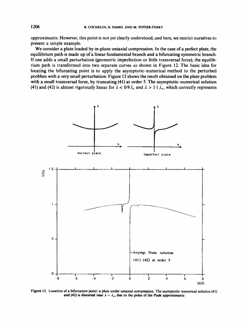
approximants. However, this point is not yet clearly understood, and here, we restrict ourselves to present a simple example.

We consider a plate loaded by in-plane uniaxial compression. In the case of a perfect plate, the equilibrium path is made up of a linear fundamental branch and a bifurcating symmetric branch. If one adds a small perturbation (geometric imperfection or little transversal force), the equilibrium path is transformed into two separate curves as shown in Figure 12. The basic idea for locating the bifurcating point is to apply the asymptotic-numerical method to the perturbed problem with a very small perturbation. Figure 12 shows the result obtained on the plate problem with a small transversal force, by truncating (41) at order 5. The asymptotic-numerical solution (41) and (42) is almost rigorously linear for 1 < 091, and L > 1-1 A,, which correctly represents

I Perfect plate

I Imperfect plate

Asymp. Num. solution

(41) (42) at order 5

- a 6 - 4 - 2 0 2 4 6 will

Figure 12. Location of a bifurcation point: a plate under u n k d compression. The asymptotic-numend solution (41) and (42) is distortad near A = a,. due to the poles of the Padc approximants


the fundamental solution path before and after the bifurcation point. Almost all the Pade approximants that we have tested have a pole around = 1,. So, the presence of persistent poles in the Pad6 approximants seems to be a good indicator for detecting a bifurcation point. Nevertheless, better asymptotic-numerical algorithms are now developed” to locate bifurcation points precisely. We have presented this example only to show the ability of the rational approximations to represent a singularity in the solution.

Remark. The existence of a pole in one Padk approximant does not necessarily indicate a bifurcation point. Particularly, nothing can be concluded when the pole is non-persistent, i.e. it moves or even disappears when the order L and M of the approximant is changed. By this example, we would only point out that all the Pad6 approximants in (41) have a persistent pole where there is a bifurcation.

5. APPLICATION TO COMPLEX NON-LINEAR BRANCHES: CONTINUATION PROCEDURES

In this section we first present the application of asymptotic-numerical methods to a non- academic problem, with a more complex geometry, a composite material and with thousands of d.0.f. in the finite element models. Second, we show that the asymptotic-numerical methods can be the basis of an efficient continuation process, which permits us to compute complex solution branches.

We consider the compressive behaviour of a delaminated composite plate which is modelled as an assembly of three Von Karman’s plates: one over delamination, one under, and the third one for the non-delaminated part.” The three plates are discretized by using 630 triangular elements and 2064 degrees of freedom. We use the classical constitutive equations of laminates with a coupling between membrane and flexion. A typical equilibrium path under compressive load is shown in Figure 13. At first, there is a linear fundamental solution without any deflection. For I = Ib , there is local buckling of the delaminated zone. Next, the global buckling of the whole laminate occurs. Let us compute such non-linear branch with asymptotic- numerical methods.

After having computed the linear fundamental solution and the first buckling mode (local buckling), we apply the method of Section 2 for computing the bifurcating branch. The result is shown in Figure 14 where we have reported the truncation of (3) at orders 15 and 16 and the improvement using Pade approximants. The whole local buckling range is obtained in one step which is satisfactory. The asymptotic numerical solution deviates from the exact one when the global buckling occurs. Once more, we have an example which shows that the asymptotic solution cannot represent a too large change of the solution’s form.

To get the remaining part of the branch, we apply a continuation procedure on the basis of the asymptotic-numerical method. The principle is very simple: we define a new starting point on the already computed part of the branch and apply the method described in Section 4. The result of this new step is shown in Figure 15 where we have again reported the truncation of(31) at orders 15 and 16 also, and the truncation of (41) and (42) at order 9. Note that a limit point in displacement has been got over. Another step is shown in Figure 16 and a summary of the continuation in Figure 17. By this way, we are able to compute a complex non-linear branch in a stepby-step manner.

A complete analytic representation of the branch has been obtained in four steps. For the same problem, we use to make about 20 steps with a classical Newton-Raphson procedure. The choice of 20 steps was not only governed by convergence requirements but also by the necessity of having a rather continuous representation of the non-linear branch.

1208 B. COCHELIN, N. DAMlL AND hi. POTIER-FERRY

36 mm 4 c

N ;; El-135 OOO Mpa E2- 8 500 Mpa v12= 0.317 G12= 5 1 5 0 Mpa F= 30 N / ~ ~ I I Stacking sequence : Lo/o~4s/o/o/-45/o/90]s

delamination Ply thickness: 0.12 mm Four edges hinged

30 -

20 - ' t /

i I 1-

/

k 1

I T - 4 4 3 2 I ,I I ? 3 L 5

N

Figure 13. A typical equilibrium path of a delaminated composite plate under compressive load

The computing time for one step of the present asymptotic-numerical method is small. Indeed, there is only one stiffness matrix decomposition, and several constructions of r.h.s. and for- ward-backward substitutions. For comparisons, the computing time for one step at order p is about the same as for one step of a modified Newton--Raphson process with p iterations. When the number of d.0.f. is very large, most of the computing time is spent by the matrix decomposition and the method requires just a little, additional time as compared to a linear calculation.

ASY MITOTIC-NUMERICAI. METHODS 1209

P=! 60

5G

40

33

20

10

0

Exact ------ Rationd repremmtion (41) (42) at order 9

\ 1- -

Polynomidl represrntntion ( 3 1 ) J I order IS -

Bifurcation point f

- 4 - 3 - 2 . ! 0 1 2 3 4 W

Figure 14. The method of Section 2 is applied for computing the bifurcating branch. The curves correspond to the truncation of the series (3) at orders 15 and 16, and of the series (24) at order 9 (Pade approximants). The whole local

buckling range is obtained in one step

60

50

40

30

20

', 0

3

1 - -.-. Exact (41) (42) at order 9 ------ - . - -1

----- __

(31) at order I5

I I I 1 1 I 1 1 I

.4 w -.4 - .3 -2 .. 1 0 1 2 .3

Figure 15. Having defined a starting point (uo, j.,,), the method of Section 4 is applied for computing a further part of the branch. The curves correspond to the truncation of the serin (31) at orders IS and 16, and of the series (41) at order 9

1210

5 0 -

40 -

30 -

20 -

10 -

0

B. COCHELIN, N. DAMIL AND hi. POTIRR-FERRY

- ----. - . . -- __ (41) (42) at order 9 \ ----------

/ I I I

60 , I I I I I

W

Figure 16. Another step of the continuation process. The curves always correspond to the truncation of the series (31) at orders I 5 and 16, and of the series (41) at order 9

60

50

40

30

20

10

0

-- %-..- TI

I I I I I I I

I I I 4 - 3 - 2 - 1 0 1 2 3 4 5

W

Figure 17. In summary, the complex non-linear branch has been obtained within four steps

ASYMPTOTIC-NUMERICAL METHODS 121 1

A very important advantage of the asymptotic-numerical method is in making the automatization of the continuation process easier. Let us detail this last point. In a classical predictorsorrector method, one must first choose a step length and then compute a new point of solution. The step length should not be too large, to avoid the divergence of the iterative process, but also not too small, to avoid inefficiency. The choice of a proper step length is crucial and, however, still difficult to automatize. In the asymptotic-numerical approach, the user must first compute the terms of the asymptotic expansions, and then analyse the range of validity of the asymptotic solution and define a new starting point. No choice of a step length has to be made a priori. The step length is analysed a posteriori either with classical criterion for determining radius of convergence* or simply by computing residual vector R(u,L) for given values of a. If the problem is poorly non-linear, the step length is naturally large. If it is strongly non-linear. it is shorter. Because the step length is not a priori chosen, but a posteriori determined, the challenge of having a robust automatic continuation method is easier with the asymptotic-numerical concept than with the prcdictorxorrector one.”

6. CONCLUSIONS

In this paper, we have applied asymptotic-numerical methods for computing the non-linear behaviour of elastic structures. The principle of the method is to compute numerically two polynomial series that give the displacement and the load as a function of a parameter a. By using a mixed approach, the governing equations have been written with a quadratic non-linearity. Hence, the expansion procedures are simple, and the method can be easily implemented in an existing FE software. A key point is that a very large number of terms of the series can be computed.

The computed series have generally a finite radius of convergence which limits the validity of the representation to a neighbourhood of the starting point (uo, Lo). However, performing an orthogonalization of the vectors ui and replacing the power series by rational fractions (Pad6 approximants), we have been able to build up a continuation of the solution branch outside the radius of convergence. Spectacular improvements of the solution have been obtained with cheap additional computations. So, we are able to get a large part of the solution branches by inverting only one matrix.

In summary, the first results are very promising. The asymptotic-numerical approach has the following advantages:

0 The computing time is small. 0 The range of validity of the expansion is often large. 0 The solution branch is known analytically and not only on some points. 0 The computation of the series is fully automatic.

Furthermore, the asymptotic-numerical methods can be applied iteratively in a step-by-step manner, in order to determine complex solution branches. The important point is that the step length is not chosen a priori by the user, but it is determined a posteriori by analysing the series. This could be the most important advantage from the view of automating non-linear computations.

Additional tests on industrial plate and shell problems are scheduled now. We are also trying to extend the asymptotic-numerical method for large rotations, for non-linear dynamics and physical non-linearities.

1212 B. COCHELIN. N. DAMlL AND M. POTIER-FERRY

APPENDIX

In Section 2, we have presented an asymptotic- numerical method to compute bifurcating branches solution of a quadratic functional equation written in the form (1). In Section 4, we have proposed a variant to compute the generic solution branches of a general quadratic functional equation (27) in the following form:

LU + Q(u,u) = If Our aim is to establish that in some cases, the framework (1) of Section 2 can be deduced from (27). For this purpose, let us assume the existence of a fundamental branch ur(I) of (27):

L W ) + Q ( U ( ( 4 , U d A ) ) = if (43) If we introduce in (27), the classical change of variable of bifurcation theory,

u = uf(j.) + Q

the new unknown Q is a solution of

Lil + 2Q(uf(i.), Q ) + Q ( Q , il) = 0 (44)

Let us remark that, if the quadratic term Q(uf().),uf(l.)) in (43) is small, i.e. if the prebuckling behaviour is linear, we get

u&) = i L - 'f = IuF (45)

This is rigorously exact for plates under in-plane compression and a common approximation for cylindrical shells under pressure.22 Using the linear approximation for the fundamental branch (49, equation (44) can be written within the framework (1):

LQ + 21 Q(UF, c) + ~ ( a , n) = o (46)

01

where the linear operators L t and L', are given by

tl(.) = L ( . ) + 2i,Q(uF;)

L; ( . ) = 2Q(uF;)

REFERENCES

I . E. Riks, 'An incremental approach to the solution of snapping and buckling problems', fn t . J. Solids Struct., 15, 529-551 (1979).

2. E. Ramm, 'Strategies for tracing the nonlinear response near limit points', in Nonlinear Finite Element Analysis in Structural Mechunics, in W. Wunderlich. E. Stein, and K. J. Bathe (eds.), Springer-Verlag Berlin, 63 89 (1981)

3 M . A. Criesfield, 'An arc-length method including line search and acceleration', f n t . j . numer. methads eng., 19.

4. N. Damil and M. Potier-Ferry, 'A new method to compute perturbed bifurcations: Application to the buckling of

5. L. Azrar, B. Cochelin, N. Damil and M. Potier-Ferry, 'An asymptotic-numerical method to compute the postbuckling

6. H. Pade, 'Sur la reprkntation approchic d'une fonction par des fractions rationnelles,' Ann. de PEcole N o m l e Sup,

7. G . A. Baker and P. Graves-Morns, Pade Approximants. Part I : Basic Theory; Encyclopedia of Mathematics and its

8. M. Van Dyke. 'Computer-extended series', Ann. Rev. Fluid Mech.. 16, 287-309 (1984).

1269-1289 (1983).

imperfect elastic structures', Int. J. E M . Sci., 28, 943-957 (1990).

behaviour of elastic plates and shells,' fnt. j. numer. methods eng., 36, 1251-1277 (1993).

3 sh ie , 9(Supp), 3-93 (1892).

applications, Vol. 13. Addison- Wesley, 1981.

ASY M PTOTIC-NUMERICAL METHODS 121 3

9. A. K. Noor and J. M. Peters, 'Reduced basis technique for nonlinear analysis of structures', A I A A J., 18, 455-462

10. E. F. Masur and H. L. Schreyer, 'A second order approximation to the problem of elastic instability', Proc. Symp.

I I . J. M. T. Thompson and A. C. Walker, 'The nonlinear perturbation analysis of discrete structural systems', Int. J.

I?. J. J. Connor and N. Morin, 'Perturbation techniques in the analysis ofgeometrically nonlinear shells', Proc. Symp. on

13. R. H. Gallagher, 'Perturbation procedures in nonlinear finite element structural analysis', C o m p u m h d M e c h -

14. 1. W. Glaum, T. Belytschko and E. F. Masur, 'Buckling of structures with finite prebuckling deformations-a

15. W. T. Koiter, 'On the stability ofelastic equilibrium', Thesis, Delft 1945, English translation NASA Tech. Trans., F. 10,

16. B. Budiansky, 'Theory of buckling and post-buckling behaviour of elastic structures', Adu. Appl. Mech., 14, 1-65

17. M. Potier-Ferry, 'Foundations of elastic post-buckling theory', in Buckling and Post-buckling, Lecture Notes in

18. Signorini, 'Sulle deformazioni termoelastiche finite', in Proc 3rd Int. Cong. Appl. Mech. No 2, 1930, pp. 80-89. 19. E. H. Boutyour, B. Cochelin and M. Potier-Ferry, 'Calcul des points de bifurcation par une methode asymptotique-

20. B. Cochelin and M. Potier-Ferry. 'A numerical model for buckling and growth of delaminations in composite

21. B. Cochelin, 'A path following technique via an asymptotic-numerical method', (1994) (to be published). 22. N. Yamaki, Elastic Stability of Circular Cylindrical Shells, North-Holland, Amsterdam, 1984. 23. A. C. Walker, 'A non-linear FEA of shallow circular arches', Int. J. Solids Srruct., 5, 97-102 (1969).

(1980).

Theory oJShells, Donne11 Anniv. Vol., Univ. of Texas, Houston, 1967. pp. 231-249.

Solids Srruct., 4, 757-768 (1968).

High Speed Comp. of Elastic Structures, Liege, 1970.

ics- Iacture Notes in Mathematics. 4 6 1 , 7S89, Springer Verlag, Berlin (1975).

perturbation FEN, In?. J. Solids Struct., 11, 1023- 1033 (1975).

883, 1967.

(1974).

Physics, Vol. 288, 1-82, Springer, Berlin, 1987, pp. 1-82.

numcrique', Proc. I" Congrb National de Micaniyue au Maroc, 371-378, ENIM, Rabat, 1993.

laminates', Comput. Methods Appl. Mech. Eng., 89, 361-380 (1991).