Download pdf - Effects of Land Use on Threatened Species

Contributed Paper

Effects of Land Use on Threatened SpeciesMANFRED LENZEN,∗ AMANDA LANE,† ASAPH WIDMER-COOPER,‡ AND MOIRA WILLIAMS†∗Centre for Integrated Sustainability Analysis, School of Physics A28, The University of Sydney, Sydney, NSW 2006, Australia,email [email protected]

†School of Biological Sciences, A08, The University of Sydney, Sydney, NSW 2006, Australia‡School of Chemistry, F11, The University of Sydney, Sydney, NSW 2006, Australia

Abstract: There is widespread agreement that biodiversity loss must be reduced, yet to alleviate threats to

plant and animal species, the forces driving these losses need to be better understood. We searched for ex-

planatory variables for threatened-species data at the country level through land-use information instead

of previously used socioeconomic and demographic variables. To explain the number of threatened species

in one country, we used information on land-use patterns in all neighboring countries and on the extent

of the country’s sea border. We carried out multiple regressions of the numbers of threatened species as a

function of land-use patterns, and we tested various specifications of this function, including spatial auto-

correlation. Most cross-border land-use patterns had a significant influence on the number of threatened

species, and land-use patterns explained the number of threatened species better than less proximate socioe-

conomic variables. More specifically, our overall results showed a highly adverse influence of plantations

and permanent cropland, a weaker negative influence of permanent pasture, and, for the most part, a

beneficial influence of nonarable lands and natural forest. Surprisingly, built-up land also showed a con-

serving influence on threatened species. The adverse influences extended to distances between about 250 km

(plants) and 2000 km (birds and mammals) away from where the species threat was recorded, depend-

ing on the species. Our results highlight that legislation affecting biodiversity should look beyond national

boundaries.

Keywords: autocorrelation, biodiversity, cross-border land use, international legislation, multiple regression,threatened species

Efectos del Uso de Suelo sobre Especies Amenazadas

Resumen: Existe el acuerdo generalizado de que se debe reducir la perdida de la biodiversidad, pero para

aligerar las amenazas a las especies de plantas y animales, las fuerzas que dirigen a estas perdidas deben ser

mejor entendidas. Buscamos variables explicativas para datos de especies amenazadas a nivel del paıs por

medio de informacion del uso de suelo en lugar de las variables socioeconomicas y demograficas utilizadas

previamente. Para explicar el numero de especies amenazadas en un paıs, usamos informacion sobre patrones

de uso de suelo en todos los paıses circunvecinos y sobre la extension de la frontera marina del paıs. Realizamos

regresiones multiples de los numeros de especies amenazadas como una funcion de los patrones de uso de

suelo, y probamos varias especificaciones de esta funcion, incluyendo autocorrelacion espacial. La mayorıa

de los patrones de uso de suelo transfronterizo tuvieron una influencia significativa sobre el numero de

especies amenazadas, y los patrones de uso de suelo explicaron el numero de especies amenazadas que

las variables socioeconomicas. Mas especıficamente, nuestros resultados generales mostraron una influencia

sumamente adversa de plantaciones y tierras agrıcolas permanentes, una menor influencia de los pastizales

permanentes y una influencia insignificante de tierras arables y no arables y bosque natural sobre las especies

amenazadas. Las influencias adversas se extendieron a distancias entre 250 km (plantas) y 2000 km (aves y

mamıferos) de donde se registro la amenaza, dependiendo de la especie. Nuestros resultados hacen evidente

que la legislacion concerniente a la biodiversidad debe ver mas alla de las fronteras nacionales.

Palabras Clave: autocorrelacion, biodiversidad, especies amenazadas, legislacion internacional, regresionmultiple, uso de suelo transfronterizo

Paper submitted September 4, 2007; revised manuscript accepted August 27, 2008.

294Conservation Biology, Volume 23, No. 2, 294–306C©2008 Society for Conservation BiologyDOI: 10.1111/j.1523-1739.2008.01126.x

Lenzen et al. 295

Introduction

Decision makers crafting policies aimed at alleviatingthreats to plant and animal species need to know aboutthe causes of these threats (reviewed by Spangenberg2002). A number of researchers have sought to identifythese threats from a global perspective by examining dataon threatened species at the country level and searchingfor the statistical determinants of species decline. Onereason for global, rather than country-level, assessmentsis to find drivers of species threats beyond the plethoraof locally specific circumstances to inform policy makingat the national and international level.

Socioeconomic and demographic variables, such aspopulation density (McKinney 2001; Burgess et al. 2007),population growth (Forester & Machlis 1996; McKeeet al. 2003), and gross national product (GNP) (Kerr &Currie 1995; Naidoo & Adamowicz 2001) are the mostfrequently tested determinants of species loss. Many au-thors search for an inverted-U relationship, or environ-mental Kuznets curve (e.g., Stern 2003). This approachhas yielded valuable yet inconsistent results, with differ-ent explanatory variables tending to be invoked for thedecline of different taxa.

For example, McPherson and Nieswaidomy (2005)found species endemism and per capita income highlysignificant predictors of threatened birds and populationdensity a predictor of threatened mammals. Naidoo andAdamowicz (2001) demonstrated that a high degree ofendemism tends to exacerbate species imperilment, butthey found the effect of per capita GNP ambiguous inthe sense that the coefficient sign varies between thetaxonomic groups. On a global scale, Kerr and Currie(1995) found human population density is the anthro-pogenic factor most closely related to the proportion ofthreatened bird species per nation, although the num-ber of threatened mammal species is more closely tiedto per capita GNP. Pandit and Laband (2007a) foundthat the only explanatory variable that has a consistentsign in analyses of all taxonomic groups is species en-demism, and the authors acknowledge these results are“a bit unsatisfying.” Unfortunately, none of the abovestudies resembles another in their choice of functionalspecification, set of countries, or selection of explana-tory variables, so direct comparisons are not possible.

Work by Pandit and Laband (2007a, 2007b) andMcPherson and Nieswaidomy (2005) is particularly in-teresting in that it shows factors influencing speciesimperilment in one country may also influence speciesimperilment in neighboring countries. Both teams usedspatial autocorrelation to incorporate cross-border ef-fects into their regression models. Investigating suchcross-border effects is important for 2 reasons. First, al-though threatened-species data are gathered at the coun-try level, species move across national boundaries, anincongruity that country-by-country analyses cannot deal

with but that is partly overcome by incorporating cross-border effects. Second, cross-border habitat reserves sit-uated in proximity to threatened habitat may play animportant role in conservation efforts.

Given that land use has been identified as a strongand proximate cause of species threats (Naeem et al.1999; Sala et al. 2000), can species threats be explainedwell by land-use patterns? Furthermore, because country-level data on species threats are somewhat incongruentwith the cross-border ranges of species, can land-use andspecies-threat regressions be improved by incorporatingcross-border regions in the land-use variable? Followingfrom this, is it possible to establish a spatial influence, or“reach” for land-use effects on species threats?

In approaching the above questions, we sought to ad-vance previous work in the following ways. Instead ofpreviously used socioeconomic and demographic vari-ables, we used land-use information as a potential deter-minant of species threat status. We believe land use is acloser proxy for causes of biodiversity loss than, for exam-ple, population density or GNP. In Australia, even thoughhuman population density is extremely low, especially inrural areas, these areas are used intensively for croppingand grazing for export, which leads to significant biodi-versity loss (Glanznig 1995). To explain the number ofthreatened species in one country, we explicitly usedinformation on land-use patterns in all neighboring coun-tries and on the extent of the country’s sea border. Seaborders are potentially important determinants of speciesthreats because of the barrier they impose on the migra-tion of many species. A high proportion of sea bordercombined with a small country size may explain highpercentages of threatened species through the lack ofaccessible cross-border habitat.

Methods

We undertook regressions between land-use and threat-ened species at the country level. At the outset, weenumerated regression models of percentages of threat-ened species. This is nothing new (as in McPherson &Nieswaidomy 2005), except that we explored land-usepatterns as explanatory variables, instead of previouslyused socioeconomic variables. Then, to examine cross-border “spill over” threats, we explicitly incorporateddata from neighboring countries. This is not straightfor-ward. Capturing aspects of neighboring countries “mightentail adding so many explanatory variables that youjeopardize your statistical degrees of freedom” (Pandit& Laband 2007a). Furthermore, not all countries haveneighbors, and not all countries with neighbors havethe same number of neighbors. Rather than simply com-paring species number with land-use breakdowns on acountry-by-country basis, we added surrounding areas to

Conservation Biology

Volume 23, No. 2, 2009

296 Land Use and Threatened Species

a country’s area when determining the so-called effectiveland-use pattern.

As with previous authors (e.g., Kerr & Burkey 2002;McPherson & Nieswiadomy 2005; Pandit & Laband2007b), we used country-level data of the percentageof threatened species and of the percentage breakdownof total area into several land-use types. This is becausecountries differ vastly with respect to the number ofspecies recorded and with regard to their land area. Thenumber of threatened species can be expected to be highwhere many species are recorded and should generallybe higher in large countries than in small countries. Theuse of percentages controls for both effects.

Data Sources

Data on land-use by country were sourced from on-linedatabases of the FAO Statistics Division (FAOSTAT 2004),the Global Forest Assessment database (FAOSTAT 2001),and the Global Land Cover Facility (GLCF 2002). Land-use patterns were derived from these data by convertingall areas into percentages of total area. These variousdata sources were used to construct a complete break-down of total area into 8 land-use types: built-up land, per-manent crops, permanent pasture, nonpermanent arableland, timber plantations, natural forest, nonarable land,and water surface. Nonarable land was calculated as theremainder of total land area and land types. Similarly, wa-ter surface was calculated as the difference between totalarea and total land area.

The adjacency matrix b (Cliff & Ord 1981) used inregressions 12 and 13 was constructed by placing theborder length in kilometers of each country i with allits neighbors j in cells bij. Information on the lengthof international borders and coast lines was taken fromthe CIA’s World Factbook (Central Intelligence Agency2006).

Data on the number of threatened plants, mammals,birds, reptiles, amphibians, and fishes were taken fromthe IUCN Red List of Threatened Species (2006). Threat-ened species are those listed as critically endangered(CR), endangered (EN), or vulnerable (VU). To convertall species numbers into percentages, we used the num-ber of total species recorded in each of the taxonomicgroups, as reported in World Resources Institute (2005).

Our analysis was carried out on the set of those coun-tries that were completely covered by all data sources.This “largest common” set comprised 153 countries.Countries that needed to be excluded, because they didnot appear in all data sets, were mostly small island na-tions. See Supporting Information for more detail on datasources used.

Cross-Border Land Use: the “Effective” Pattern

Consider a country C of total area AC surrounded by othercountries and water (Fig. 1). This country will have a cer-

tain composition AC,i of land use of i = 1,. . .,L types(including water bodies) AC = ∑L

i=1 λi AC = ∑Li=1 AC,i ,

where λi is the percentage of each surface type i in thetotal area AC. Let �rC(l) be a radial vector originating fromthe country’s geometrical center of gravity and l be an arcvariable measuring the progression on the dashed circles.Extend the inner circle by a distance dr = |d�r| toward theouter circle, thus including some of the areas surround-ing the country. In general these surrounding areas willhave a different composition λ = {λi} compared with C.Ideally, the λi are continuous functions λi(l,R), and �R =�rC(l) + d�r is the extended radial variable (dr = |d�r| is thelength of the vector d�r). The total area Ai of type i in aring of width dr is a line integral along the perimeters ofthe circles

Ai(R) =∫

l

∫ rc(l)+dr

R=rc(l)λi(l, R)dRdl, (1)

where the integrand λi(l,R) dR dl is an infinitesimal areaas indicated by the hatched polygon in Fig. 1.

The “effective” area composition of country C is a vec-tor λ∗

C with elements

λ∗C ,i(R) = AC ,i + Ai(R)

AC +∑L

i=1Ai(R)

. (2)

This new composition includes all areas within a circleof radius R from C’s geometrical center of gravity. Onewould expect λ∗ to change with increasing R as newareas of generally different composition are included. Weuse the term effective area because we tested whetherareas surrounding a country are effective in determining

Figure 1. A country (C) of total area AC surrounded

by other countries and water (l, line integral variable;

d l, infinitesimal progression on line l; rC(l), radial

variable from country center to line l; dr, infinitesimal

progression on radius).


Volume 23, No. 2, 2009

Lenzen et al. 297

the percentage of threatened species in that country.In ecological terms, the area AC + ∑L

i=1 Ai(R) may beregarded as the area that species in C draw on for theirsurvival, and R is the spatial “reach” of that species.

A shortcoming of the formulation in Eq. 1 is that itcannot be evaluated because for the majority of countries,data suitable for constructing λi(l,R) are not available ona subcountry level of spatial detail. Therefore, we setλi(l,R) = λn ,i if coordinates (l,R) fell within country n.

Some examples may help demonstrate the concept ofthe effective land-use pattern. Consider Namibia with anarea of 8.2 million km2 and a perimeter of 5500 km.About 43% of Namibia is nonarable arid land, and about46% is permanent pasture, with the remaining land-usetypes playing minor roles (Table 1, top row, R = 0).Nevertheless, most of Namibia’s neighbors, such as An-gola, Zambia, and Botswana, feature significant naturalforests. When expanding a circle beyond Namibia’s bor-ders, these forests are increasingly included in the effec-tive land-use pattern at the expense of nonarable land(Table 1, second and third row, R = 750 km and R =1500 km).

The effective land-use pattern can be interpreted in thecontext of cross-border effects on species threats. For ex-ample, any threat to species in Namibia’s 10% of naturalforest could likely be absorbed by habitat across the bor-der in Angola, Botswana, and Zambia, so the natural forestaffecting forest species is effectively larger at around 15%.Conversely, any habitat destruction in forests in Angola,Botswana, and Zambia could lead to threatened speciesbeing recorded in Namibia.

The change in the effective land-use pattern is more ex-treme for small countries. For Bhutan surrounding arableland has overtaken forest in the effective land-use pattern

Table 1. Effective land-use pattern λC,i∗(R) for 5 countries, 8 land-use types, and 3 radii R.

Built-upa Permanent Permanent Nonpermanent Timber Natural Nonarable Water

Country R (km) (%) crops (%) pasture (%) arable landb (%) plantations (%) forest (%) landc (%) surface (%)

Namibia 0 0.1 0.0 46.1 1.0 0.0 9.8 42.9 0.1Namibia 750 0.2 0.0 34.7 1.0 0.0 15.2 24.8 24.1Namibia 1500 0.3 0.2 29.6 3.0 0.2 16.0 10.2 40.6Bhutan 0 1.6 0.4 8.8 2.3 0.4 63.7 22.7 0.0Bhutan 200 2.7 1.0 29.2 12.2 3.5 29.1 20.1 2.2Bhutan 500 4.9 1.8 23.6 28.1 5.8 14.3 16.2 5.3Singapore 0 33.1 1.5 0.0 1.5 0.6 2.2 59.7 1.5Singapore 50 11.6 6.3 0.3 2.3 2.0 18.5 25.0 33.9Singapore 100 4.3 4.3 0.2 1.5 1.3 12.8 10.7 65.0Fiji 0 1.9 4.7 9.6 10.9 5.3 39.3 28.3 0.0Fiji 150 0.4 1.1 2.2 2.5 1.2 8.9 6.4 77.4Fiji 300 0.2 0.5 1.0 1.2 0.6 4.3 3.1 89.1Australia 0 0.1 0.0 51.5 6.2 0.1 19.8 21.5 0.8Australia 1500 0.1 0.0 41.6 5.0 0.1 16.0 17.3 19.9Australia 3500 0.1 0.2 11.6 1.7 0.2 6.8 5.5 73.9

aLand used for settlements and infrastructure.bRotations of grazing, cropping, and fallow.cDesert, ice, etc.

at 500-km reach. Similarly, a 100-km wide circle aroundthe center of Singapore contains a far smaller proportionof built-up (urban) land than Singapore itself, but mostlywater to the south, and natural forest to the north inMalaysia. In the case of small and remote islands such asFiji, all terrestrial surface categories decrease at the ex-pense of water surface with increasing corridor depth.For an island continent such as Australia, however, thiseffect is nowhere near as pronounced and only starts atR >1000 km reach. This size dependence of the effec-tive land-use pattern is a meaningful feature that makeslarge countries far less influenced by smaller surroundingcountries than vice versa.

Effective areas were calculated by scanning country-centered circles of varying radii R on a digitized map ofthe world (Fig. 2). In constructing these circles, we firstapplied the projection equation to translate pixel posi-tions on the map into latitude and longitude. Second, weapplied the cosine rule of spherical geometry to translateangular coordinates into distances between 2 points.

Of course, the approach outlined earlier has weak-nesses. First, it assumes land-type percentages are a ho-mogeneous characteristic of a country’s entire area, eventhough in reality, the near-border region of a neighbormay have only one land type present. In addition, it doesnot recognize terrestrial barriers for species migration.For example, those regions of Chile closest to the Argen-tinean border are almost entirely made up of nonarablemountain ranges. Similarly, the threatened species areassumed to be homogeneously dense across the coun-try, whereas in reality there may be so-called hotspotsconcentrated in some subnational areas (Dobson et al.1997), and these hotspots might or might not be close toa border.


Volume 23, No. 2, 2009


Figure 2. Digitization of (a) world map demarcating an area to show effective land-use pattern by country. Each

grid cell holds a number representative of a country and (b) shows a detail of gray circle in (a). Circle is centered

in The Netherlands (no. 137) and includes areas of Belgium (19), Germany (73), Luxembourg (114), France (67),

and ocean (0).

Analyses

We tested a variety of specifications for multiple regres-sions of percentages of threatened species against land-use patterns:

S =7∑

i=1

βiλ∗i + εi . (3)

The coefficients βi in Eq. 3 can be interpreted as char-acterization factors for land-use types. If land-use type 2were permanent cropland, then β2 = 0.3 would meanthat in a hypothetical large area completely covered withpermanent cropland, 30% would be threatened. Undis-turbed landforms are characterized by β = 0. Such char-acterization factors are often used in life-cycle assessment(LCA) to represent the impact category land use (e.g.,Lindeijer 2000). In Eq. 3 and all following regressions,the ε i are uncorrelated errors, normally distributed withmean 0.

S = β0 +7∑

i=1

βiλ∗i + εi . (4)

Equation 4 (used by McPherson & Nieswiadomy 2005;Pandit & Laband 2007a, 2007b) is similar but less intu-itive because it assumes a “background” threat β0, whichexists independent of any land use, that is in a completelyundisturbed world.

S =7∑

i=1

βiλ∗i + β8λ

∗8 + εi . (5)

Equation 5 is similar to Eqs. 3 and 4, but includes watersurfaces (type 8) in addition to land types (types 1–7).

log(S) = β0 +7∑

i=1

βi log(λ∗

i

) + εi . (6)

Equation 6 is used, for example, by Naidoo andAdamowicz (2001); the coefficients βi are elasticitiesβi = ∂Sλ∗

i /S∂λ∗i that describe the relative change in S

as a consequence of relative changes in the λ∗i . Such

elasticities are used, for example, in response functionsof temporal analyses (Eppink et al. 2004; Zebisch et al.2004).

log(S) =7∑

i=1

βi log(λ∗

i

) + εi (7)

and

log(S) =7∑

i=1

βi log(λ∗

i

) + β8log(λ∗

8

) + εi . (8)

Equations 7 and 8 are similar, but exclude the constantand include water surfaces, respectively.

√S =

7∑i=1

βi log(λ∗

i

) + εi , (9)

√S = β0 +

7∑i=1

βi log(λ∗

i

) + εi , (10)


Volume 23, No. 2, 2009

Lenzen et al. 299

and

√S =

7∑i=1

βi log(λ∗

i

) + β8log(λ∗

8

) + εi . (11)

Equations 9, 10, and 11 incorporate the square-rootspecification used by Kerr and Burkey (2002). Both log-and square-root forms are used in the literature to stabilizevariances of species numbers, if these happened to behigher than those of explanatory variables. In Eqs. 3–11,λ∗

i= λ∗

i(R) vary with reach R.

S = β0 + ρbnS +7∑

i=1

βiλi + εi (12)

and

log(S) = β0 + ρlog(bnS) +7∑

i=1

βi log(λi) + εi . (13)

Finally, Eq. 12 is the spatial lag model as specified byMcPherson and Nieswaidomy (2005), and Eq. 13 is itslogarithmic version. In agreement with these authors, weused a normalized adjacency matrix bn to model spillovereffects in this regression (instead of the effective land-use pattern). As a consequence this analysis is only “onelayer of neighbors deep.” Initially, all equations except 12and 13 were evaluated with both ordinary and weightedleast squares (OLS/WLS), with the weights modeled as thesquare roots of absolute numbers of threatened species toaccount for the heteroscedasticity of country-level data.The WLS regressions were subsequently discarded be-cause weights were correlated with the explained vari-ables (see Supporting Information). Equations 12 and 13were only evaluated with maximum likelihood (ML) es-timation because of the bias in least-squares estimators(Anselin 1988:58). The ML estimator was enumerated ac-cording to solution procedure for the mixed-regressivespatial-autoregressive model (Anselin 1988:180–182).

A number of authors (e.g., McPherson & Nieswiadomy2005) argue that the threats posed to species by deforesta-tion have been around much longer than species records,so there may be countries with a currently low rate ofdeforestation and threatened species because most de-forestation and extinction happened in the past and littleforest and few species remain to be wiped out. We con-sidered this circumstance by excluding countries with ahigh per capita income that typically populate the de-clining inverted-U branch of a Kuznets curve for environ-mental pressure. Turning points of inverted-U curves varydepending on what environmental pressure type is ex-amined. For deforestation, turning points vary betweenGDP/capita of $1500 and $9000, depending on the statis-tical specification (Koop & Tole 1999). In one regressionexperiment we therefore excluded all countries with aper capita GDP above $9000.

None of the socioeconomic or other explanatory fac-tors found by other authors—such as endemism and rar-ity, population density, or per capita GNP—were takeninto account. This was a deliberate omission because wesought to characterize land use as an exhaustive explana-tory variable set for species threats.

Results

Spatial Autocorrelation

The results of the spatial autocorrelation tests (see Sup-porting Information) were unanimous in that Geary’s c

(Geary 1954) and Moran’s I (Moran 1948) confirmed pos-itive spatial autocorrelation and the autocorrelation coef-ficients of the spatial lag models were all positive. Never-theless, the sign of the remaining land-use coefficients ofthe regressions were rather inconsistent. We believe thisshortcoming is due to the fact that all spatial effects werecontained within the autocorrelated term in Eqs. 12 and13. In the following, we examine whether moving thespatial autocorrelation effect into the land-use variablesby using the effective (cross-border) land-use pattern willyield more intuitive results.

Regression

Before carrying out regression analyses, we confirmedthat none of the variables showed prohibitive multi-collinearity. In fact, none of the correlation coefficients(absolutes) among the land-use percentages or the threat-ened species percentages exceeded 0.5, and most ofthem were around 0.15.

We performed ordinary least-squares (OLS) regres-sion analyses with Eqs. 3–13 against the land-use pat-tern λi

∗(R) included inside reach R. We were inter-ested in whether regressions against the effective land-use patterns λi

∗(R) would perform better than regres-sions against the country-specific land-use patterns λi =λi

∗(R = 0), and if so, at what R. Figure 3 shows detailedresults of such an analysis for Eq. 10 (the square-rootspecification used in Kerr and Burkey [2002]).

The effective land-use pattern was a better predictorfor countries’ threatened species than the countries’ ownland-use pattern (Fig. 3) because for most of the species,we observed a peak in the R2 values around 300 km ≤Rmax ≤ 3000 km. In other words, there was a distanceat which the cross-border effects were most effectivein terms of species threats. This indicates that includinga certain area of neighboring countries into the effectiveland-use patterns better explained threatened species andat some distance, land-use patterns ceased to affect threat-ened species.


Volume 23, No. 2, 2009


Figure 3. The efficacy of the effective land-use pattern to explain the number of threatened species in a country as

a function of distance from its center. Plotted are the normalized determination coefficients R2/ R2max from

ordinary least-squares regression analysis of the relationship specified in Eq. 10 for all taxa.

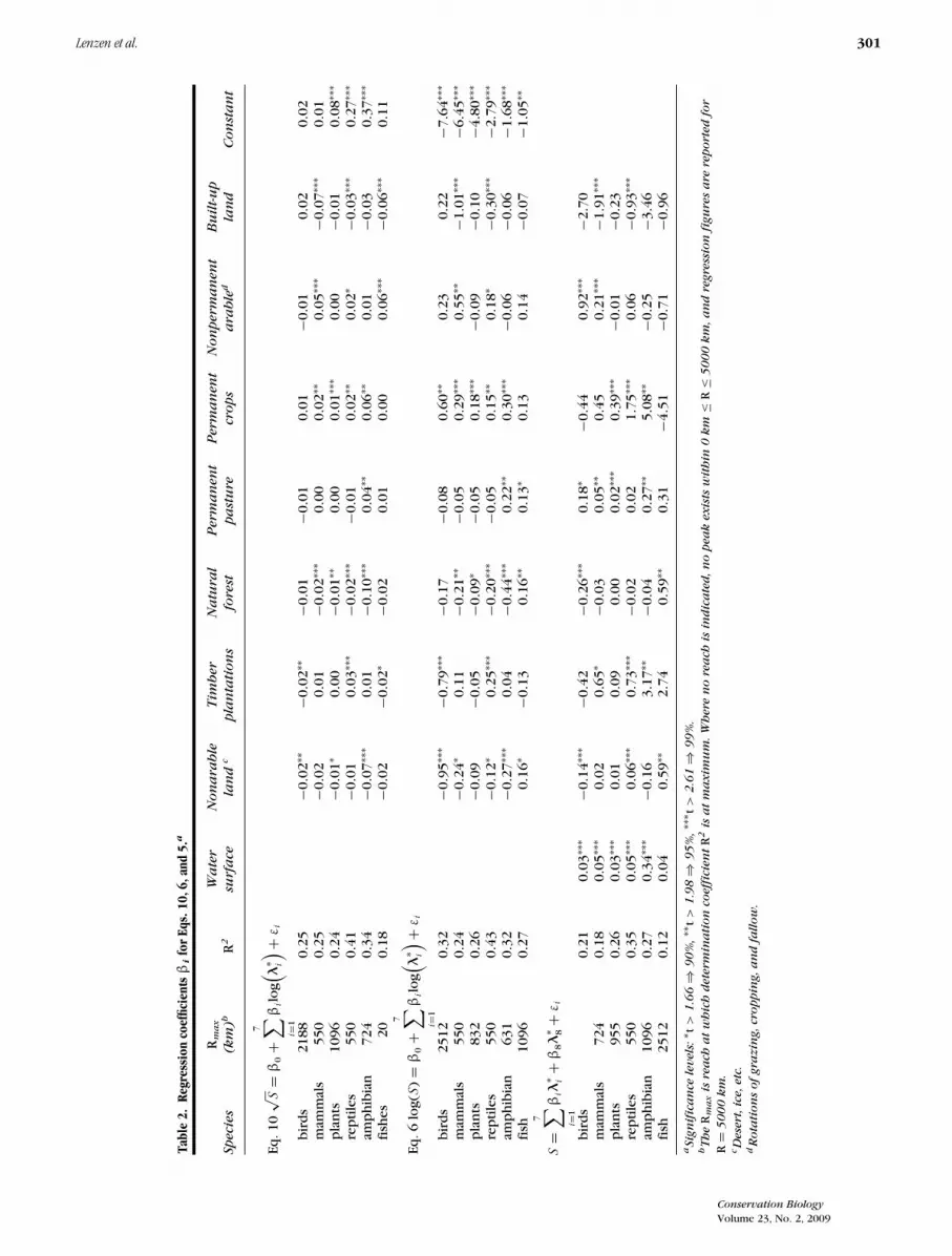
In the regression coefficients, we called positive coeffi-cients threatening and negative coefficients conserving

to avoid the normative connotations of the terms pos-

itive and negative. Equations 10 (square-root specifica-tion of Kerr and Burkey [2002]), 6 (logarithmic speci-fication of Naidoo and Adamowicz [2001]), and 5 (lin-ear specification of McPherson and Nieswaidomy [2005]and Pandit and Laband [2007a, 2007b], but includingocean surfaces) yielded highly significant threatening in-fluences of permanent cropland on all species exceptfishes (Table 2). Nonpermanent arable land, permanentpasture, and timber plantations were also significantlythreatening in some cases. The linear specification clearlyshowed the influence of the water barrier for vulnerablespecies on isolated islands. The influence of natural for-est and nonarable land on threatened species was consis-tently conserving, except for 2 coefficients for fishes andsome small positive coefficients in Eq. 5. Surprisingly,built-up land also resulted in conserving influences.

The category plants (all threats) was dominated by thestatus rare, which is not necessarily a consequence ofland-use patterns. In addition, the category all species

combined species with quite different reaches and land-use vulnerabilities. We therefore omitted these categoriesin Table 2 and in all following results. With regard tofishes, the reaches resulting from the 2 regressions inTable 2 did not match, and the regression coefficientsdid not align well with those of other species. This isnot surprising because land-use does not affect fishes asmuch as terrestrial species. We therefore also excludedfishes from all following results.

Table 3 provides the absolute R2 values and regres-sion coefficients and levels of significance for all Eqs.3–11 for the 3 taxa covered by a large number of recordswith small variations in the percentage of threats: birds,mammals, and plants. Characterization factors |βi| >1

occurred in Eqs. 3–5 for birds and mammals, but onlyfor the land type built-up land. With the exception ofsmall countries, such as Singapore, built-up land usuallycomprised around 1% of country areas in our data set(Supporting Information). Hence, these characterizationfactors must be seen as applicable for marginal changesand not applicable for a scenario that, for example, hasall land built up at once.

Regressions yielded a mixed bag. For birds (Table 3,top), permanent cropland, nonpermanent arable land,and permanent pasture were associated with significantcoefficients and threatening influences, whereas naturalforest and nonarable land were associated with oftensignificant conserving influences. Counter to intuition,built-up land and to a lesser extent timber plantationsyielded significant conserving influences. Water surfaceresulted in significant threatening influence whenever itwas part of the specification, which—for peak R2 valuesat between Rmax = 2200 km and 5000 km—highlightsthe vulnerability of birds on isolated islands.

For mammals the picture was much more consistent.Regressions yielded almost only threatening coefficients,many of them significant, for permanent crops, nonper-manent arable land, permanent pasture, and timber plan-tations and almost only conserving coefficients, many ofthem significant, for natural forest and non-arable land.Once again, built-up land produced a surprising con-serving influence on species. Mammalian peak reaches,at around 600 km, were much lower than avian peakreaches.

For plants (Table 3, bottom), the peak reach Rmax

was also low at around 800 km, which reflects the re-stricted mobility of plants (compare with Devictor &Jiguet [2007] and references therein). The coefficientsfor permanent cropland remained threatening and sig-nificant and those for natural forest and nonarable land


Volume 23, No. 2, 2009

Lenzen et al. 301

Tabl

e2.

Regr

essi

onco

effic

ient

sβ

ifo

rEq

s.10

,6,a

nd5.

a

Rm

ax

Wa

ter

Non

ara

ble

Tim

ber

Na

tura

lP

erm

an

en

tP

erm

an

en

tN

on

perm

an

en

tB

uil

t-u

p

Speci

es

(km

)bR

2su

rfa

cela

nd

cpla

nta

tion

sfo

rest

pa

stu

recr

ops

ara

ble

dla

nd

Con

sta

nt

Eq.1

0√

S=

β0+

7 ∑ i=1

βil

og( λ

∗ i

) +ε

i

bir

ds

2188

0.25

−0.0

2∗∗−0

.02∗∗

−0.0

1−0

.01

0.01

−0.0

10.

020.

02m

amm

als

550

0.25

−0.0

20.

01−0

.02∗∗

∗0.

000.

02∗∗

0.05

∗∗∗

−0.0

7∗∗∗

0.01

pla

nts

1096

0.24

−0.0

1∗0.

00−0

.01∗∗

0.00

0.01

∗∗∗

0.00

−0.0

10.

08∗∗

∗

rep

tile

s55

00.

41−0

.01

0.03

∗∗∗

−0.0

2∗∗∗

−0.0

10.

02∗∗

0.02

∗−0

.03∗∗

∗0.

27∗∗

∗

amp

hib

ian

724

0.34

−0.0

7∗∗∗

0.01

−0.1

0∗∗∗

0.04

∗∗0.

06∗∗

0.01

−0.0

30.

37∗∗

∗

fish

es20

0.18

−0.0

2−0

.02∗

−0.0

20.

010.

000.

06∗∗

∗−0

.06∗∗

∗0.

11

Eq.6

log(

S)=

β0+

7 ∑ i=1

βil

og( λ

∗ i

) +ε

i

bir

ds

2512

0.32

−0.9

5∗∗∗

−0.7

9∗∗∗

−0.1

7−0

.08

0.60

∗∗0.

230.

22−7

.64∗∗

∗

mam

mal

s55

00.

24−0

.24∗

0.11

−0.2

1∗∗−0

.05

0.29

∗∗∗

0.55

∗∗−1

.01∗∗

∗−6

.45∗∗

∗

pla

nts

832

0.26

−0.0

9−0

.05

−0.0

9∗−0

.05

0.18

∗∗∗

−0.0

9−0

.10

−4.8

0∗∗∗

rep

tile

s55

00.

43−0

.12∗

0.25

∗∗∗

−0.2

0∗∗∗

−0.0

50.

15∗∗

0.18

∗−0

.30∗∗

∗−2

.79∗∗

∗

amp

hib

ian

631

0.32

−0.2

7∗∗∗

0.04

−0.4

4∗∗∗

0.22

∗∗0.

30∗∗

∗−0

.06

−0.0

6−1

.68∗∗

∗

fish

1096

0.27

0.16

∗−0

.13

0.16

∗∗0.

13∗

0.13

0.14

−0.0

7−1

.05∗∗

S=

7 ∑ i=1

βiλ

∗ i+

β8λ

∗ 8+

εi

bir

ds

0.21

0.03

∗∗∗

−0.1

4∗∗∗

−0.4

2−0

.26∗∗

∗0.

18∗

−0.4

40.

92∗∗

∗−2

.70

mam

mal

s72

40.

180.

05∗∗

∗0.

020.

65∗

−0.0

30.

05∗∗

0.45

0.21

∗∗∗

−1.9

1∗∗∗

pla

nts

955

0.26

0.03

∗∗∗

0.01

0.09

0.00

0.02

∗∗∗

0.39

∗∗∗

−0.0

1−0

.23

rep

tile

s55

00.

350.

05∗∗

∗0.

06∗∗

∗0.

73∗∗

∗−0

.02

0.02

1.75

∗∗∗

0.06

−0.9

3∗∗∗

amp

hib

ian

1096

0.27

0.34

∗∗∗

−0.1

63.

17∗∗

−0.0

40.

27∗∗

5.08

∗∗−0

.25

−3.4

6fi

sh25

120.

120.

040.

59∗∗

2.74

0.59

∗∗0.

31−4

.51

−0.7

1−0

.96

aSig

nif

ica

nce

levels

:∗ t

>1

.66

⇒9

0%

,∗∗

t>

1.9

8⇒

95

%,

∗∗∗ t

>2

.61

⇒9

9%

.bTh

eR

ma

xis

rea

cha

tw

hic

hdete

rmin

ati

on

coeff

icie

nt

R2

isa

tm

axim

um

.W

here

no

rea

chis

indic

ate

d,n

opea

kexis

tsw

ith

in0

km

≤R

≤5

00

0km

,a

nd

regre

ssio

nfi

gu

res

are

report

ed

for

R=

50

00

km

.cD

ese

rt,ic

e,etc

.dR

ota

tion

sof

gra

zin

g,cr

oppin

g,a

nd

fallow

.


Volume 23, No. 2, 2009


Tabl

e3.

Regr

essi

onco

effic

ient

sβ

ifo

rEq

s.3–

11fo

rbi

rds,

mam

mal

san

dpl

ants

.a

Model

Rm

ax

Wa

ter

Non

ara

ble

Tim

ber

Na

tura

lP

erm

an

en

tP

erm

an

en

tN

on

perm

an

en

tB

uil

t-u

p

equ

ati

on

(km

)bR

2su

rfa

cela

nd

cpla

nta

tion

sfo

rest

pa

stu

recr

ops

ara

ble

dla

nd

Con

sta

nt

Bir

ds 3

200.

170.

01∗

0.00

0.01

∗∗0.

000.

14∗∗

∗−0

.02∗∗

0.03

450

120.

21−0

.17∗∗

∗−0

.43

−0.2

9∗∗∗

0.16

−0.4

80.

90∗∗

∗−2

.74

0.03

∗∗∗

550

120.

210.

03∗∗

∗−0

.14∗∗

∗−0

.42

−0.2

6∗∗∗

0.18

∗−0

.44

0.92

∗∗∗

−2.7

06

2512

0.32

−0.9

5∗∗∗

−0.7

9∗∗∗

−0.1

7−0

.08

0.60

∗∗0.

230.

22−7

.64∗∗

∗

738

020.

17−0

.42

−0.3

20.

40−1

.37∗∗

∗2.

36∗∗

∗−2

.31∗∗

0.99

∗

850

120.

372.

83∗∗

∗−1

.19∗∗

−0.3

1−0

.93∗∗

2.75

∗∗∗

2.23

∗∗∗

3.12

∗∗−3

.38∗∗

∗

921

880.

25−0

.02∗∗

−0.0

2∗∗∗

−0.0

1−0

.01

0.01

0.00

0.02

1021

880.

25−0

.02∗∗

−0.0

2∗∗−0

.01

−0.0

10.

01−0

.01

0.02

0.02

1150

120.

280.

06∗∗

∗−0

.07∗∗

∗−0

.02

−0.0

9∗∗∗

0.12

∗∗∗

0.01

0.19

∗∗∗

−0.1

1∗∗∗

Mam

mal

s3

170.

100.

03∗

0.25

∗∗0.

010.

03∗

0.29

∗∗∗

0.03

−0.1

14

724

0.18

−0.0

30.

60∗

−0.0

8∗∗∗

0.00

0.40

0.16

∗∗−1

.96∗∗

∗0.

05∗∗

∗

572

40.

180.

05∗∗

∗0.

020.

65∗

−0.0

30.

05∗∗

0.45

0.21

∗∗∗

−1.9

1∗∗∗

655

00.

24−0

.24∗

0.11

−0.2

1∗∗−0

.05

0.29

∗∗∗

0.55

∗∗−1

.01∗∗

∗−6

.45∗∗

∗

7n

op

eak

0.11

0.43

∗∗∗

0.34

∗∗∗

0.40

∗∗∗

0.43

∗∗∗

0.31

∗∗∗

−0.0

9−0

.25

8n

op

eak

0.28

0.12

0.31

∗∗0.

31∗∗

∗0.

57∗∗

∗0.

37∗∗

∗0.

34∗∗

∗0.

02−0

.42∗∗

955

00.

25−0

.02∗

0.01

∗−0

.02∗∗

∗0.

000.

02∗∗

0.05

∗∗∗

−0.0

8∗∗∗

1055

00.

25−0

.02

0.01

−0.0

2∗∗∗

0.00

0.02

∗∗0.

05∗∗

∗−0

.07∗∗

∗0.

0111

550

0.24

0.00

−0.0

2∗0.

01−0

.02∗∗

∗0.

000.

02∗∗

0.05

∗∗∗

−0.0

8∗∗∗

Pla

nts 3

200.

210.

02∗∗

∗0.

040.

02∗∗

∗0.

01∗∗

∗0.

17∗∗

∗−0

.01

0.03

495

50.

26−0

.02∗∗

∗0.

06−0

.03∗∗

∗−0

.01

0.37

∗∗∗

−0.0

4∗−0

.26∗

0.03

∗∗∗

595

50.

260.

03∗∗

∗0.

010.

090.

000.

02∗∗

∗0.

39∗∗

∗−0

.01

−0.2

36

832

0.26

−0.0

9−0

.05

−0.0

9∗−0

.05

0.18

∗∗∗

−0.0

9−0

.10

−4.8

0∗∗∗

70.

03−0

.41

−0.2

90.

04−1

.40∗∗

∗1.

71∗∗

∗0.

130.

028

0.23

1.17

∗∗∗

−0.0

90.

18−0

.19

0.77

∗1.

25∗∗

∗0.

49−1

.30∗∗

∗

90.

22−0

.05∗∗

∗−0

.01

−0.0

7∗∗∗

0.04

∗∗0.

010.

11∗∗

∗−0

.05∗∗

∗

1010

960.

24−0

.01∗

0.00

−0.0

1∗∗0.

000.

01∗∗

∗0.

00−0

.01

0.08

∗∗∗

110.

220.

00−0

.05∗∗

∗−0

.01

−0.0

7∗∗∗

0.04

0.00

0.11

∗∗∗

−0.0

5∗∗

aSig

nif

ica

nce

levels

:∗ t

>1

.66

⇒9

0%

,∗∗

t>

1.9

8⇒

95

%,

∗∗∗ t

>2

.61

⇒9

9%

.bR

ea

cha

tw

hic

hdete

rmin

ati

on

coeff

icie

nt

R2

isa

tm

axim

um

.N

oen

try

or

“no

pea

k”

un

der

Rm

ax

indic

ate

sn

opea

kexis

tsw

ith

in0

km

≤R

≤5

00

0km

.In

the

case

of

no

en

try,R

2im

pro

ves

wit

hin

crea

sin

gre

ach

,a

nd

regre

ssio

nfi

gu

res

are

report

ed

for

R=

50

00

km

.“N

opea

k”

indic

ate

sre

gre

ssio

ns

dete

riora

tew

ith

incr

ea

sin

gre

ach

.cD

ese

rt,ic

e,etc

.dR

ota

tion

sof

gra

zin

g,cr

oppin

g,a

nd

fallow

.


Volume 23, No. 2, 2009

Lenzen et al. 303

conserving and significant. Nonpermanent arable land,permanent pasture, and timber plantations showed am-biguous coefficient patterns. Most of the coefficients forwater surfaces were once again threatening and signifi-cant, and most of those for built-up land once again indi-cated conserving influences.

With respect to their magnitude, the coefficients ofregressions 3–5, 6–8, and 9–10 could not be comparedamong each other because of the influence of the squareroots and logarithms. Nevertheless, the significance andsigns of OLS regression coefficients were relatively con-sistent across species when averaged over all equations(Table 4). The significant threatening influence of perma-nent crops stood out most of all, followed by the clearconserving role of natural forest and the threatening ef-fect of ocean borders. Less significant but still consistentwere the threatening influences of nonpermanent arableland, permanent pasture, and timber plantations and theconserving influence of nonarable land. Both persistentand surprising was the clear negative sign of coefficientsfor built-up land. Amphibians appeared to be the onlyspecies that were significantly threatened by processesindependent of land-use patterns, reflected in the highlysignificant constant term (compare Beebee & Griffiths2005; Cushman 2006). The peak reaches for the vari-ous species broadly reflected their mobility, with plants,mammals, and amphibians at the lower end and birds atthe upper end of the range.

The coefficient signs in Table 4 were as expected forall land-use types except built-up land. We investigatedwhether spurious effects could have caused the negativesign for this land type. First, we excluded outlier coun-tries such as Singapore with a high percentage of built-up land from the analysis. Second, we tested a Kuznets-type hypothesis by excluding countries above various percapita GDP thresholds from the analysis, hoping to iso-late the increasing inverted-U branch with a threateningcoefficient (see the Analyses section for details). Third,we examined whether positive coefficients for built-upland exist for effective land-use patterns with radii otherthan the documented optimum reach (see SupportingInformation). Fourth, we excluded ocean surfaces fromthe land-use pattern and ran specifications 3, 7, and 9with the remaining 7 explanatory variables. None of thesechecks yielded any evidence of a positive-sign coefficientfor built-up land. Hence, the negative-sign coefficientsin Table 4 must be seen as genuine and not caused byregression-technical circumstances.

Discussion

The majority of our results show that cross-border land-use patterns have a significant influence on speciesthreats and that land-use patterns are a more proximatecause for threats than previously used socioeconomic Ta

ble

4.Re

gres

sion

resu

ltsav

erag

edov

erEq

s.3–

11.a

Rm

ax

Wa

ter

Non

ara

ble

Tim

ber

Na

tura

lP

erm

an

en

tP

erm

an

en

tN

on

perm

an

en

tB

uil

t-u

p

Speci

es

(km

)bsu

rfa

cela

nd

cpla

nta

tion

sfo

rest

pa

stu

recr

ops

ara

ble

dla

nd

Con

sta

nt

Bir

ds

2201

4.79

∗∗∗

−2.6

8∗∗∗

−1.5

8−2

.08∗∗

0.38

2.27

∗∗1.

23−0

.76

−0.3

0M

amm

als

440

2.15

∗∗−0

.21.

99∗∗

−0.7

11.

202.

25∗∗

2.14

∗∗−4

.02∗∗

∗−1

.03

Pla

nts

796

5.41

∗∗∗

−1.6

3−0

.19

−2.3

5∗∗0.

183.

80∗∗

∗0.

45−2

.00∗∗

−0.3

4R

epti

les

1439

1.40

−0.0

12.

96∗∗

∗−2

.42∗∗

−0.6

13.

16∗∗

∗1.

14−2

.83∗∗

∗1.

19A

mp

hib

ian

564

2.32

∗∗−2

.22∗∗

0.63

−2.9

2∗∗∗

2.12

∗∗2.

43∗∗

−0.0

8−0

.99

2.62

∗∗∗

aTh

eta

ble

show

sva

lues

for

ta

lon

gw

ith

the

sign

of

the

coeff

icie

nt

an

dth

ele

velof

sign

ific

an

ce.

bTh

eR

ma

xis

rea

cha

tw

hic

hdete

rmin

ati

on

coeff

icie

nt

R2

isa

tm

axim

um

(com

pa

reA

ppen

dix

S2

).La

nd

types

an

dsi

gn

ific

an

cele

vels

as

inTa

ble

2.

cD

ese

rt,ic

e,etc

.dR

ota

tion

sof

gra

zin

g,cr

oppin

g,a

nd

fallow

.


Volume 23, No. 2, 2009


variables (e.g., Thompson & Jones 1999; Burgess et al.2007). This is important because land use is dynamic(White et al. 1997) and thus may more easily be integratedinto conservation decisions. Managing land-use patternsand intensity can in principle be done more directly, im-mediately, and practically and has more immediate effectsin terms of habitat conservation and regeneration than,for example, influencing GNP and population density.There may also be scope for reducing the pressure onbiodiversity through land-use changes without adverselyaffecting GNP and settlements. Such decoupling wouldprofoundly change the results of regression specificationsin earlier work, but not the land-use specifications as wehave defined them.

More specifically, our results illustrate a generally highand adverse influence of permanent cropland, planta-tions, and nonpermanent arable land, a weaker influ-ence of permanent pasture, and a beneficial influence ofnonarable lands and natural forest on threatened species.These findings concur with patterns observed on both lo-cal and regional scales, which demonstrates the negativeimpacts on biodiversity of deforestation (e.g., Allan et al.1997) and conversion to croplands (Zapfack et al. 2002).

The negative relationship between threatened speciesand built-up land is surprising given the acknowledgedthreat of urbanization to biodiversity (Czech et al. 2000;McKinney 2006). This overall result could be a combina-tion of a positive relationship for low-income countries,followed by a negative relationship for wealthy countries(an inverted-U or Kuznets form). By excluding wealthycountries from the regression, we tested 2 hypotheses:wealthy countries expend more funds on the protectionof habitat and threatened species, thus leading to lowernumbers of threatened species, and wealthy countrieshave less species to threaten to begin with because themost vulnerable species have already become extinct. Wedid not find any evidence for a positive-sign coefficientfor built-up land to support either of our hypotheses. Thisissue requires further investigation.

A conserving influence of built-up land on threatenedspecies numbers is consistent with previous work con-ducted on a regional scale in Belgium (Honnay et al.2003), which demonstrated a positive influence of per-centage built-up area on both total species number andthe number of threatened species. The authors partly at-tributed the result to a high diversity of niches availablein urban areas due to varying disturbance and nutrientregimes. Lower-intensity management of agricultural landremaining in suburban areas was also thought to providespecialized habitat for rare and threatened plants. Intrica-cies associated with managing native remnants withinurban areas will heavily influence the potential valueof these environments as habitat for threatened species;hence, speculating on the reason for our finding is likelyto be more fruitful when analyses are conducted at thelandscape level.

Our results provide clear and direct evidence that us-ing land-use data from surrounding countries allows fora better prediction of threats to biodiversity. This is in-tuitive because species, and the ecosystem processes onwhich they depend, are not bounded by national bor-ders. The level of threat to biodiversity is likely to be afunction of the surrounding land use in an ecologicallyrelevant geographical area (e.g., as defined by dispersaldistances within plants or migratory patterns in birds).The finding that the relevant geographic areas that shouldbe considered differs across taxa is also intuitive; mobilespecies such as birds and mammals depend on a largergeographic area than sessile plants, and there is muchempirical evidence to support this (e.g., Thiollay 1989;Agetsuma 2007).

That said, the relevant geographical areas we proposeshould not be interpreted as the dispersal distances ofindividual taxa. Although dispersal capabilities are im-portant, our findings also incorporate factors that affectthe entire ecosystem on which species depend. By way ofexample, the conversion of forest to cropland is likely tohave many indirect impacts in addition to the direct dis-placement of animals. Cropping can influence water qual-ity (Konstantinou et al. 2005), which will have effects forspecies that reside in a broader geographic area. The rea-son the adverse influences of land-use extend such largedistances in our study (600 km for plants and 2000 km forbirds) is likely due to a combination of species dispersalabilities and the influence of the ecosystem functions onwhich species depend.

Taxa were grouped together into broad categories forour analysis (e.g., mammals, birds, plants); therefore, wewere unable to account for the large amount of variationin the physical extent of land on which particular speciesdepend, even within relatively closely related taxonomicgroups. There is great variability in the behavior of in-dividual species, and habitat generalists are expected tobe more affected by land use across a broader regioncompared with habitat specialists (Clobert et al. 2001).

Despite these limitations, our results provide a generalrule of thumb that can be applied in a conservation man-agement and planning context. The influence of land-usechange will not only depend on the amount of land beingconverted but also on the nature of the land-use matrixthat is produced as a result. The importance of fragmenta-tion and the nature of the juxtaposition of habitats haveimportant consequences for species persistence (Hans-son & Angelstram 1991).

A significant influence of cross-border patterns on bio-diversity also highlights the need for extending conser-vation legislation across national boundaries (comparewith Spangenberg 2002). Our findings support the ef-forts of existing international treaties (e.g., Conventionon International Trade in Endangered Species of WildFauna and Flora [CITES]) and may be able to furtherinform them. Encouraging cross-border approaches to


Volume 23, No. 2, 2009

Lenzen et al. 305

conservation biology is more relevant than ever as globalwarming necessitates the development of wildlife cor-ridors to allow migration into more climate-appropriateareas (e.g., the corridor joining the Selous game reservein Tanzania with the Niassa game reserve in Mozambique[Ngwature & Hahn 2006]). Our estimates of relevant ge-ographic area might appear to be on the large side, butgiven changes in species range expected with climatechange, this is likely to be prudent.

Supporting Information

A list of countries (Appendix S1) and further details of theautocorrelation and regression calculations (AppendixS2) are available as part of the on-line article. The authoris responsible for the content and functionality of thesematerials. Queries (other than absence of the material)should be directed to the corresponding author.

Literature Cited

Agetsuma, N. 2007. Minimum area required for local populations ofJapanese Macaques estimated from the relationship between habi-tat area and population extinction. Journal of Primatology 28:97–106.

Allan, D. G., J. A. Harrison, R. A. Navarro, B. W. Van Wilgen, and M. W.Thompson. 1997. The impact of commercial afforestation on birdpopulations in Mpumalanga province, South Africa—insights frombird-atlas data. Biological Conservation 79:173–185.

Anselin, L. 1988. Spatial econometrics: methods and models. Kluwer,Dordrecht, The Netherlands.

Beebee, T. J. C., and R. A. Griffiths. 2005. The amphibian decline cri-sis: A watershed for conservation biology? Biological Conservation125:271–285.

Burgess, N. D., A. Balmford, N. J. Cordeiro, J. Fjeldsa, W. Kuper, C.Rahbek, E. W. Sanderson, J. W. Scharlemann, J. H. Sommer, andP. H. Williams. 2007. Correlations among species distributions, hu-man density and human infrastructure across the high biodiversitytropical mountains of Africa. Biological Conservation 134:164–177.

Central Intelligence Agency (CIA). 2006. The world factbook. CIA,Washington, D.C.

Cliff, A., and J. Ord. 1981. Spatial processes, models and applications.Pion, London.

Clobert, J., E. Danchin, A. A. Dhondt, and J. D. Nichols. 2001. Dispersal.Oxford University Press, Oxford, United Kingdom.

Cushman, S. A. 2006. Effects of habitat loss and fragmentation onamphibians: a review and prospectus. Biological Conservation128:231–240.

Czech, B., P. R. Krausman, and P. K. Devers. 2000. Economic associa-tions among causes of species endangerment in the United States.BioScience 50:593–601.

Devictor, V., and F. Jiguet. 2007. Community richness and stabilityin agricultural landscapes: the importance of surrounding habitats.Agriculture, Ecosystems and Environment 120:179–184.

Dobson, A. P., J. P. Rodriguez, W. M. Roberts, and D. S. Wilcove. 1997.Geographic distribution of endangered species in the United States.Science 275:550–553.

Eppink, F. V., J. C. J. M. Van Den Bergh, and P. Rietveld. 2004. Modellingbiodiversity and land use: urban growth, agriculture and nature in awetland area. Ecological Economics 51:201–216.

FAOSTAT (FAO Statistics Division). 2001. Forested area. Food and Agri-culture Organisation of the United Nations (FAO), Rome.

FAOSTAT (FAO Statistics Division). 2004. Land use—2002. Food andAgriculture Organisation of the United Nations (FAO), Rome.

Forester, D. J., and J. E. Machlis. 1996. Modelling human factors thataffect the loss of biodiversity. Conservation Biology 10:1253–1263.

Geary, R. 1954. The contiguity ratio and statistical mapping. The Incor-porated Statistician 5:115–145.

Glanznig, A. 1995. Native vegetation clearance, habitat loss and biodi-versity decline. Department of the Environment, Sport and Territo-ries Biodiversity Unit, Canberra, Australia.

Global Land Cover Facility (GLCF). 2002. Modis satellite imagery:forested area. University of Maryland, College Park.

Hansson, L., and P. Angelstram. 1991. Landscape ecology as a theoreticalbasis for nature conservation. Landscape Ecology 5:191–201.

Honnay, O., K. Piessens, W. Van Landuyt, M. Hermy, and H. Gulinck.2003. Satellite based land use and landscape complexity indices aspredictors for regional plant species diversity. Landscape and UrbanPlanning 63:241–250.

Kerr, J. T., and T. V. Burkey. 2002. Endemism, diversity, and the threatof tropical moist forest extinctions. Biodiversity and Conservation11:695–704.

Kerr, J. T., and D. J. Currie. 1995. Effects of human activity on globalextinction risk. Conservation Biology 9:1528–1538.

Konstantinou, I. K., D. G. Hela, and T. A. Albanis. 2005. The status ofpesticide pollution in surface waters of Greece. Part I. Review onoccurrence and levels. Environmental Pollution 141:555–570.

Koop, G., and L. Tole. 1999. Is there an environmental Kuznets curvefor deforestation? Journal of Development Economics 58:231–244.

Lindeijer, E. 2000. Biodiversity and life support impacts of land use inLCA. Journal of Cleaner Production 8:313–319.

McKee, J. K., P. W. Sciulli, C. D. Fooce, and T. A. Waite. 2003. Forecast-ing global biodiversity threats associated with human populationgrowth. Biological Conservation 115:161–164.

McKinney, M. L. 2001. Role of human population size in raising birdand mammal threat among nations. Animal Conservation 4:54–57.

McKinney, M. L. 2006. Urbanization as a major cause of biotic homog-enization. Biological Conservation 127:247–260.

McPherson, M. A., and M. L. Nieswiadomy. 2005. EnvironmentalKuznets curve: threatened species and spatial effects. EcologicalEconomics 55:395–407.

Moran, P. 1948. The interpretation of statistical maps. Journal of theRoyal Statistical Society B 10:243–251.

Naeem, S., et al. 1999. Biodiversity and ecosystem functioning: main-taining natural life support processes. Issues in Ecology 4:1–11.

Naidoo, R., and W. L. Adamowicz. 2001. Effects of economic prosperityon numbers of threatened species. Conservation Biology 15:1021–1029.

Ngwature, I. N., and H. R. Hahn. 2006. Selous–Niassa wildlife cor-ridor: Ruvuma investment forum October 2006. Selous–NiassaWildlife Corridor/UNDP-GEF/GTZ-IS, Namtumbo, Tanzania.Available from http://www.selous-niassa-corridor.org/fileadmin/publications/SNWC_Ruvuma_Investment_Forum_2006.pdf (ac-cessed September 2008).

Pandit, R., and D. N. Laband. 2007a. General and specific spatial auto-correlation: insights from country-level analysis of species imperil-ment. Ecological Economics 61:75–80.

Pandit, R., and D. N. Laband. 2007b. Spatial autocorrelation in country-level models of species imperilment. Ecological Economics 60:526–532.

Sala, O. E., et al. 2000. Global biodiversity scenarios for the year 2100.Science 287:1770–1774.

Spangenberg, J. H. 2002. Environmental space and the prism of sus-tainability: frameworks for indicators measuring sustainable devel-opment. Ecological Indicators 2:295–309.

Stern, D. I. 2003. The rise and fall of the Environmental Kuznets Curve.Rensselaer Polytechnic Institute, Troy, New York.


Volume 23, No. 2, 2009


IUCN (International Union for Conservation of Nature). The IUCN redlist of threatened species. 2006. Summary statistics for globallythreatened species. Table 5: threatened species in each country(totals by taxonomic group). IUCN, Cambridge, United Kingdom.

Thiollay, J. M. 1989. Area requirements for the conservation of rainforestraptors and game birds in French Guiana. Conservation Biology3:128–137.

Thompson, K., and A. Jones. 1999. Human population density andprediction of local plant extinctions in Britain. Conservation Biology13:185–190.

White, D., P. G. Minotti, M. J. Barczak, J. C. Sifneos, K. E. Freemark,M. V. Santelmann, C. F. Steinitz, A. R. Kiester, and E. M. Preston.

1997. Assessing risk to biodiversity from future landscape change.Conservation Biology 11:349–360.

World Resources Institute (WRI). 2005. WRI biodiversity overview.WRI, Washington, D.C.

Zapfack, L., S. Engwald, B. Sonke, G. Achoundong, and B. Madong.2002. The impact of land conservation on plant biodiversity in theforest zone of Cameroon. Biodiversity and Conservation 11:2047–2061.

Zebisch, M., F. Wechsung, and H. Kenneweg. 2004. Landscape re-sponse functions for biodiversity—assessing the impact of land-usechanges at the county level. Landscape and Urban Planning 67:157–172.


Volume 23, No. 2, 2009