
arX
iv:1
410.
5474
v1 [
nlin
.CD
] 2
Jun
201
4
Ermakov Systems with Multiplicative Noise
E. Cervantes-Lopez a, P.B. Espinoza a, A. Gallegos a,H.C. Rosu b
aDepartamento de Ciencias Exactas y Tecnologıa, Centro Universitario de los
Lagos, Universidad de Guadalajara, Enrique Dıaz de Leon 1144, Col. Paseos de la
Montana, Lagos de Moreno, Jalisco, Mexico
bDivision of Advanced Materials, IPICyT, 78231 San Luis Potosı, S.L.P., Mexico
Physica A 401 (2014) 141-147
• Multiplicative noise is introduced in the Ermakov systems of equations.
• The noise is added in the Euler-Maruyama numerical scheme.
• No effect found in the Ermakov invariant only when noise is put in both equations.
• Lewis-Riesenfeld phases show a small shift effect for reasonable noise amplitudes.
Abstract
Using the Euler-Maruyama numerical method, we present calculations of theErmakov-Lewis invariant and the dynamic, geometric, and total phases for severalcases of stochastic parametric oscillators, including the simplest case of the stochas-tic harmonic oscillator. The results are compared with the corresponding numericalnoiseless cases to evaluate the effect of the noise. Besides, the noiseless cases areanalytic and their analytic solutions are briefly presented. The Ermakov-Lewis in-variant is not affected by the multiplicative noise in the three particular examplespresented in this work, whereas there is a shift effect in the case of the phases.
Key words: Ermakov-Lewis invariant; Euler-Maruyama method; multiplicativenoise; total phase; geometric phase; dynamic phase
Email addresses: [email protected] (E. Cervantes-Lopez),[email protected] (P.B. Espinoza), [email protected] (A.Gallegos), [email protected] (H.C. Rosu).
Preprint submitted to Elsevier 22 October 2014

1 Introduction
Noisy harmonic oscillators are widely used simple models with many appli-cations in physics, chemistry, biology, medicine, economics and sociology andhave been recently reviewed in the book of Gitterman [1]. On the other hand,it is well established that integrals of motion and dynamical invariants arerelated to the symmetries of the conservative dynamical systems and many ofthem have well-established phenomenological meaning. In particular, an in-variant quantity introduced by Ermakov [2] a long time ago and reobtained byLewis [3] by another method and in a different context has become a standardconcept in the dynamical analysis of the important class of parametric oscil-lator systems. These systems are widespread in many areas of physics such assemiclassical theory of radiation, mechanical oscillations with time-dependentparameters, motion of charged particles in certain types of magnetic fields,cosmological models, and so on (see [4] and references therein). In general,such kinds of systems are described by the following Newton type equation ofmotion
x+ Ω2(t)x = 0 , (1)
where Ω(t) is the time-dependent frequency. One can write the solution of (1)in the Milne form [5]
x(t) = Cρ(t) sin (ΘT (t) + φ) . (2)
C and φ are arbitrary constants and the phase ΘT (t) is given by
ΘT (t) =
t∫ 1
ρ2(t′)dt′ (3)
and ρ(t) is a solution of the Milne-Pinney equation
ρ+ Ω2(t)ρ =k
ρ3, (4)
where k is an arbitrary real constant. It is also known how to express thefunction ρ in terms of two linearly independent solutions of the x oscillator[4].
For parametric oscillators governed by Eqs. (1) and (4) forming a so-calledErmakov system, one can introduce the Ermakov-Lewis invariant [2,3] given
2

by the following formula [6] (henceforth we use k = 1)
I =1
2(ρx− ρx)2 +
1
2
(
x
ρ
)2
. (5)
Moreover, the total phase ΘT is the sum of a pure dynamical phase and ageometric phase. The latter is a rather common concept for time-dependentsystems ever since it has been introduced by Berry in 1984 in a quantum-mechanical context [7]. In the case of classical mechanical systems these geo-metric phases are also called Hannay angles [8]. The dynamical phase is relatedto the dynamical nature of the evolution of the system, while the geometricphase depends on the geometry and topology of the phase space trajectory asa function of the variation of the parameters of the system. The dynamic andgeometric phases [4,9,10] are given by the following equations (henceforth weuse k = 1)
∆Θd(t) =
t∫
[
1
ρ2−
1
2
d
dt′(ρρ) + ρ2
]
dt′ (6)
and
∆Θg(t) =
t∫
[
1
2
d
dt′(ρρ)− ρ2
]
dt′ . (7)
By examining the last two formulas, one can notice that their sum is indeed thetotal phase. Notice also that for a constant ρ the geometric phase is naught.
2 Stochastic calculus
Although there is a huge literature on the Ermakov systems there are onlya couple of papers on the Ermakov approach for stochastic oscillators. Inthe 1980’s, Nassar introduced an Ermakov-Nelson stochastic process in thehydrodynamic interpretation of the Schroedinger equation [11], while in 2005Haas [12] used the Haba-Kleinert averaging method [13] for the stochasticquantization of time-dependent systems.
Motivated by this scarcity and also by the natural question of how robust arethe Ermakov quantities of the parametric oscillator (1) to stochastic noises,we present here a study of the effects of the multiplicative noise on the Er-makov quantities. The noise will be taken as a Brownian random walk noise in
3
the framework of the theory of stochastic processes [14]. This theory has beenvery supportive in modeling phenomena that do not exactly follow a continu-ous path and have small disturbances when they evolve in noise-perturbativeconditions.
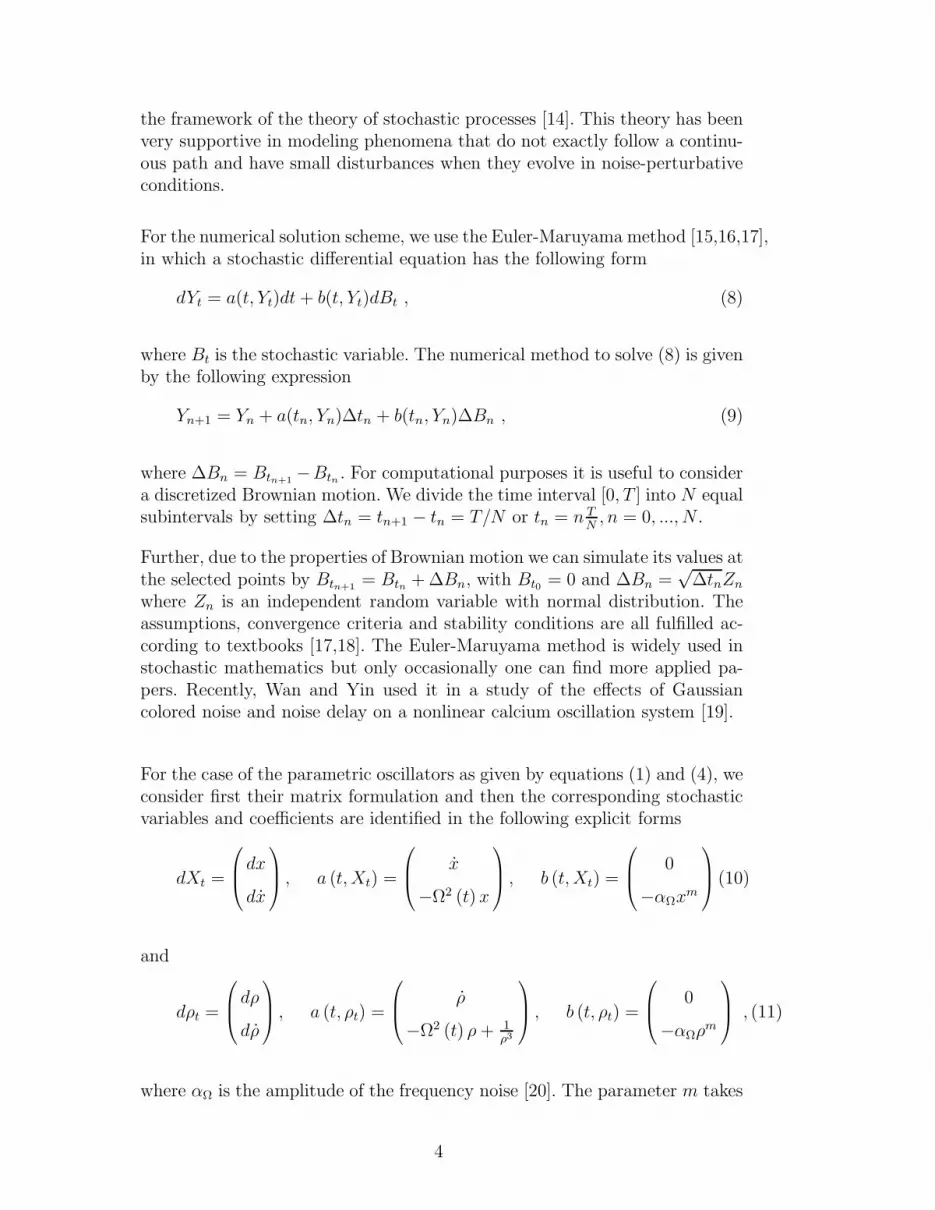
For the numerical solution scheme, we use the Euler-Maruyama method [15,16,17],in which a stochastic differential equation has the following form
dYt = a(t, Yt)dt+ b(t, Yt)dBt , (8)
where Bt is the stochastic variable. The numerical method to solve (8) is givenby the following expression
Yn+1 = Yn + a(tn, Yn)∆tn + b(tn, Yn)∆Bn , (9)
where ∆Bn = Btn+1−Btn . For computational purposes it is useful to consider
a discretized Brownian motion. We divide the time interval [0, T ] into N equalsubintervals by setting ∆tn = tn+1 − tn = T/N or tn = n T
N, n = 0, ..., N .
Further, due to the properties of Brownian motion we can simulate its values atthe selected points by Btn+1
= Btn +∆Bn, with Bt0 = 0 and ∆Bn =√∆tnZn
where Zn is an independent random variable with normal distribution. Theassumptions, convergence criteria and stability conditions are all fulfilled ac-cording to textbooks [17,18]. The Euler-Maruyama method is widely used instochastic mathematics but only occasionally one can find more applied pa-pers. Recently, Wan and Yin used it in a study of the effects of Gaussiancolored noise and noise delay on a nonlinear calcium oscillation system [19].
For the case of the parametric oscillators as given by equations (1) and (4), weconsider first their matrix formulation and then the corresponding stochasticvariables and coefficients are identified in the following explicit forms
dXt =
dx
dx
, a (t, Xt) =
x
−Ω2 (t) x
, b (t, Xt) =
0
−αΩxm
(10)
and
dρt =
dρ
dρ
, a (t, ρt) =
ρ
−Ω2 (t) ρ+ 1
ρ3
, b (t, ρt) =
0
−αΩρm
, (11)
where αΩ is the amplitude of the frequency noise [20]. The parameter m takes
4

the value 0 for the additive noise and can be any positive integer number biggerthan the unity for the multiplicative cases. Of course, one can use any functiong(x) and g(ρ) instead of xm and ρm to study more general couplings of thenoise [21]. Unfortunately, it is easy to see that the additive noise case leads toparametric equations of the form x + Ω2(t)x = ξ and ρ+ Ω2(t)ρ = k
ρ3+ ξ for
which the expression of the Ermakov-Lewis invariant is more complicated [22].This is due to the fact that the noise term occurs as a true forcing term and notas a contribution to the time-dependent frequency parameter. Moreover, thecalculations for the formulas of the dynamic and geometric phases involve aux-iliary equations related to the forcing term. Thus this case is left for a futureinvestigation. Besides, for m > 1 the oscillators have amplitude-dependent fre-quencies and therefore although they could be still called parametric they arenonlinear in the frequency too and the Ermakov-Lewis approach in this caseis still under development. Therefore only the m = 1 multiplicative case willbe considered in the applications to follow because for this case the standardErmakov-Lewis analysis holds. For this case, the noise appears as a randomeffect in time on the time-dependent frequency.
In addition, as one can see from (10) and (11), we use the same noise term inthe two oscillators of the Ermakov system. In our numerical calculations, wealso studied cases containing the noise either only in the linear oscillator (10)or the nonlinear one (11). For these cases, independently of the used seed, wehave seen a stronger effect of the noise on the Ermakov-Lewis invariant. Forillustration purposes, this feature is presented in the first application belowbut similar plots have been obtained in the other two applications. Besides,we have seen the same shifting effect on the phases in the presence of noise inthe ρ oscillator and no effect at all when the noise was in the linear oscillator,as expected because the phases depend only on the ρ function. On the otherhand, we noticed an interesting compensating effect of the noise terms in theErmakov-Lewis invariant when the same noise is added in both oscillators.
3 Applications
We move now to three explicit applications for which we follow Eliezer andGray [6] and use the initial conditions x(0) = 1, x(0) = 0 for the solutionof (1), which imply similar initial conditions for the Milne-Pinney solution:ρ(0) = 1 and ρ(0) = 0.
5

3.1 Harmonic oscillator
We choose first the particular case of the pure harmonic oscillator with Ω0 = 2and present the effect of the multiplicative noise on the EL invariant andthe three phases in Fig. (1). One can see that the general effect is a smallshift proportional with the amplitude of the noise. For ρ we use the followingformula obtained by Eliezer and Gray using an auxiliary plane motion [6]
ρ =
√
x2(t) +h2
α2x22(t) , (12)
where h is an arbitrary constant playing the role of the constant angularmomentum and
x(t) = αx1(t) + βx2(t) (13)
is the general harmonic solution which satisfy the initial conditions x(0) = αand x(0) = β. In this paper, we choose α = 1 and β = 0 as initial conditionsand fix the constant h to unity, which means that we use a quadrature formulafor ρ
ρ(t) =√
x21(t) + x2
2(t) . (14)
The corresponding harmonic solutions are x1 = cos Ω0t and x2 = 1
Ω0sin Ω0t
and it can be easily shown that the Milne-Pinney function of the pure harmonicoscillator which fulfills the initial conditions ρ(0) = 1 and ρ(0) = 0 is
ρ(t) =
√
(Ω20 − 1) cos2Ω0t + 1
Ω0
, (15)
which for Ω0 = 2 reduces to ρ(t) = 1
2
√3 cos2 2t+ 1.
For completeness, in Fig. (2) we present the Ermakov-Lewis invariant for theharmonic Ermakov system with the noise included in only one of the oscilla-tors. For these asymmetric cases, we have always obtained a more visible effectof the noise on the Ermakov-Lewis invariant which for us serves as evidencethat the correct procedure is to include the noise on equal footing in bothequations of the Ermakov systems.
6

3.2 Parametric oscillator with Ω(t) = 2 sin t
The plots of the Ermakov quantities for this case are displayed in Fig. (3).The effect of the noise is similar to the previous case.
For completeness, we also present the analytic solution of this parametricoscillator. The corresponding parametric equation can be easily shown to beof the following Mathieu type
x+ (2− 2 cos 2t)x = 0 . (16)
The solutions satisfying the initial conditions as given by Eliezer and Gray are
x1(t) =C(2, 1; t)
C(2, 1; 0), x2(t) =
S(2, 1; t)
S(2, 1; 0), (17)
where C(2, 1; 0) ≈ 1.182 and S(2, 1; 0) ≈ 0.5336 and the C and S functions arethe known Mathieu cosine and Mathieu sine functions and their Wronskian isW = 1. Therefore, the analytic Milne-Pinney solution fulfilling the same initial
conditions as x1 has implicitly the quadrature format ρ(t) =√
x21(t) + x2
2(t).
3.3 Parametric oscillator with Ω(t) = 2t2
This case can be found in the list of analytic cases given by Eliezer and Grayin their paper. We provide here the two linearly independent solutions of theparametric equation which satisfy the Eliezer-Gray initial conditions:
x1(t) =Γ(
5
6
)
31
6
√tJ
−1
6
(
2t3
3
)
, x2(t) =Γ(
1
6
)
2 · 35
6
√tJ 1
6
(
2t3
3
)
. (18)
Their Wronskian is W = 1 and therefore one can obtain the Milne-Pinneyfunction from an equation of the same form as (14). The plots of the Ermakovquantities for this case are presented in Fig. (4). The slight shift effect of thenoise is again noticeable.
4 Concluding remarks
We have studied the effects of the simplest type of multiplicative noise on theErmakov systems for three particular cases. The Euler-Maruyama numerical
7

scheme has been used to include the stochastic noise in the Ermakov system. Ithas been found that the usage of the same noise term in the two oscillators ofthe Ermakov system leads to a cancelation of the noise effects on the Ermakov-Lewis invariant, which can be due to the structure of the invariant itself. Onthe other hand, the effect of the noise in the nonlinear oscillator leads to ashift effect on the three phases of the system. This can be understood as aconsequence of the averaging effect produced by the integrals in the expressionsof the phases.
Acknowledgements
The authors wish to thank one of the referees whose comments led to a sub-stantial improvement of this work.
References
[1] M. Gitterman, The Noisy Oscillator: The First Hundred Years, From EinsteinUntil Now, World Scientific, Singapore, 2005.
[2] V.P. Ermakov, Univ. Izv. Kiev Series III 9 (1880) 1-25; Translation by A.O.Harin, Second order differential equations: Conditions of complete integrability,Appl. Anal. Discr. Math. 2 (2008) 123-145.
[3] H.R. Lewis Jr., C lass of exact invariants for classical and quantum time-dependent harmonic oscillators, J. Math. Phys. 9 (1968) 1976-1986.
[4] P.B. Espinoza, E rmakov-Lewis dynamic invariants with some applications,(2000), 51 pages, math-ph/0002005.
[5] W.E. Milne, The numerical determination of characteristic numbers, Phys. Rev.35 (1930) 863-867.
[6] C.J. Eliezer, A. Gray, A note on the time-dependent harmonic oscillator, SIAM(Soc. Ind. Appl. Math.) J. Appl. Math. 30 (1976) 463-468.
[7] M.V. Berry, Quantal phase factors accompanying adiabatic changes, Proc. R.Soc. A 392 (1984) 45-57.
[8] J. H. Hannay, Angle variable holonomy in adiabatic excursion of an integrableHamiltonian, J. Phys. A: Math. Gen. 18 (1985) 221-230.
[9] M. Maamache, E rmakov systems, exact solution, and geometrical angles andphases, Phys. Rev. A 52 (1995) 936-940.
8

[10] H. C. Rosu, P. B. Espinoza, E rmakov-Lewis angles for one-parameter susyfamilies of Newtonian free damping modes, Phys. Rev. E 63 (2001) 037603.
[11] A.B. Nassar, T ime-dependent harmonic oscillator: An Ermakov-Nelson process,Phys. Rev. A 32 (1985) 1862-1863.
[12] F. Haas, S tochastic quantization of time-dependent systems by the Haba andKleinert method, Int. J. Theor. Phys. 44 (2005) 1-9.
[13] Z. Haba, H. Kleinert, Schrodinger wave functions from classical trajectories,Phys. Lett. A 294 (2002) 139-142.
[14] J.L. Doob, S tochastic Processes, Wiley, New York, 1953.
[15] B.K. Oksendal, S tochastic Differential Equations: An Introduction withApplications, Springer-Verlag, Berlin, 2003.
[16] G.N. Milstein, M.V. Tretyakov, S tochastic Numerics for Mathematical Physics.Scientific Computation, Springer-Verlag, Berlin, 2004.
[17] P.E. Kloeden, E. Platen, N umerical Solution of Stochastic DifferentialEquations, in Applications of Mathematics 23, Springer-Verlag, 1992.
[18] P. Protter, S tochastic Integration and Differential Equations, second edition.Stochastic Modelling and Applied Probability 21, Springer-Verlag, Berlin, 2005.
[19] B. Wang, Z. Yin, Effects of colored noise and noise delay on a calcium oscillationsystem, Physica A 392 (2013) 4203-4209.
[20] B.K. Oksendal, S tochastic Differential Equations: An Introduction withApplications, Springer-Verlag, Berlin, 2003, p. 64.
[21] M. Gitterman, The Noisy Oscillator: The First Hundred Years, From EinsteinUntil Now, World Scientific, Singapore, 2005, pp. 15 and 45.
[22] K. Takayama, Dynamical invariant for forced time-dependent harmonicoscillator, Phys. Lett. A 88 (1982) 57-59.
9

Fig. 1. (Color online) The EL invariants in the range t ∈ [0, π] for the harmonicoscillator with Ω0 = 2 (top left) the dynamic phase (top right), geometric phase(bottom left), and total phase (bottom right). In blue, the corresponding graphics fora noiseless oscillator. The magenta colour corresponds to the m = 1 multiplicativenoise of amplitude αΩ = 0.1 and the green colour corresponds to the amplitudeαΩ = 0.2.
Fig. 2. (Color online) The EL invariants in the range t ∈ [0, π] for the harmonicoscillator with Ω0 = 2. The noise is included only in the x-oscillator (left) andonly in the ρ-oscillator (right). The magenta colour corresponds to the m = 1multiplicative noise of amplitude αΩ = 0.1 and the green colour corresponds to theamplitude αΩ = 0.2.
10
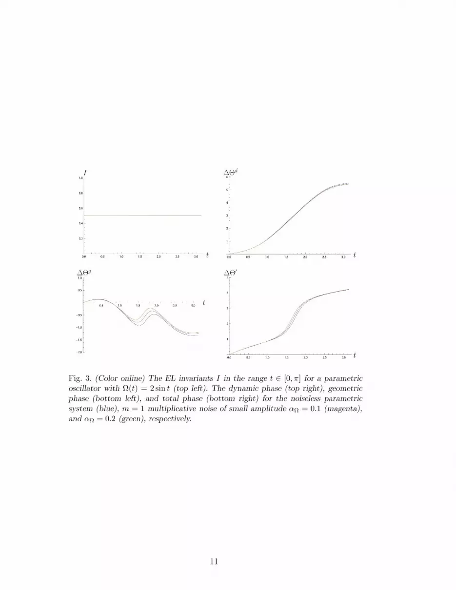
Fig. 3. (Color online) The EL invariants I in the range t ∈ [0, π] for a parametricoscillator with Ω(t) = 2 sin t (top left). The dynamic phase (top right), geometricphase (bottom left), and total phase (bottom right) for the noiseless parametricsystem (blue), m = 1 multiplicative noise of small amplitude αΩ = 0.1 (magenta),and αΩ = 0.2 (green), respectively.
11

Fig. 4. (Color online) The EL invariant I in the range t ∈ [0, π] for the parametricoscillator with Ω(t) = 2t2 (top left). The dynamic phase (top right), geometric phase(bottom left), and total phase (bottom right) for the noiseless case (blue), m = 1noise of amplitudes αΩ = 0.1 (magenta) and αΩ = 0.2 (green), respectively.
12
Recommended


