Preprint - ESSD

1

Generalized models to estimate carbon and nitrogen stocks

of organic soil layers in Interior Alaska

Kristen Manies, Mark Waldrop, Jennifer Harden

U.S. Geological Survey

345 Middlefield Rd.

Menlo Park, CA 94025 USA

Correspondence to: Kristen Manies ([email protected])

https://doi.org/10.5194/essd-2019-114

Ope

n A

cces

s Earth System

Science

DataD

iscussio

ns

Preprint. Discussion started: 6 August 2019c© Author(s) 2019. CC BY 4.0 License.

2

Abstract 1

Boreal ecosystems comprise about one tenth of the world’s land surface and contain over 20 % of 2

the global soil carbon (C) stocks. Boreal soils are unique in that the mineral soil is covered by what can be 3

quite thick layers of organic soil. These organic soil layers, or horizons, can differ in their state of 4

decomposition, source vegetation, and disturbance history. These differences result in varying soil 5

properties (bulk density, C content, and nitrogen (N) content) among soil horizons. Here we summarize 6

these soil properties, as represented by over 3000 samples from Interior Alaska, and examine how soil 7

drainage and stand age affect these attributes. The summary values presented here can be used to gap-fill 8

large datasets when important soil properties were not measured, provide data to initialize process-based 9

models, and validate model results. These data are available at https://doi.org/10.5066/P960N1F9 10

(Manies, 2019). 11

12

1 Introduction 13

Boreal soils play an important role in the global carbon (C) budget and are estimated to store 14

between 375 - 690 Pg of C (Hugelius et al., 2014; Bradshaw and Warkentin, 2015; Khvorostyanov et al., 15

2008), which is over 20 % of the global soil C stock (Jackson et al., 2017). These soils are unique in that 16

for many boreal ecosystems a large portion of this C can be found within the organic soil layer (Jorgenson 17

et al., 2013). This organic soil layer results from the relatively high input rates, through plant matter, that 18

result from the high summer solar radiation this region receives. In addition, C losses from the soil are 19

low, as cool and/or freezing soil temperatures result in low rates of decomposition. The imbalance 20

between C inputs and losses results in thick organic soils that store large amounts of C (Jorgenson et al., 21

2013). There is also considerable C found in the mineral soil of these systems, especially where protected 22

by permafrost (O'Donnell et al., 2011; Jorgenson et al., 2013). 23

Nitrogen (N) also plays an important role in boreal ecosystems due to N limitations on plant 24

growth. One of the main determinants of N availability is decomposition rates. Disturbances that increase 25


Ope

n A

cces

s Earth System

Science

DataD

iscussio

ns


3

decomposition can also increase N availability which, in turn, increases plant growth, offsetting some of 26

the C losses due to increased decomposition (Finger et al., 2016). 27

Boreal organic soils are unique when compared to soils from other regions. First, these organic 28

soils are thick, ranging from several centimeters to several meters (Ping et al., 2006). They are also 29

comprised of layers which vary in their degree of decomposition. These layers can also be formed from 30

different types of vegetation. Both factors result in soil layers of varying density. The density and 31

thickness of these organic soil layers also vary depending on the amount of time since the last disturbance 32

(Deluca and Boisvenue, 2012). In addition, C and N concentrations vary between layers, again depending 33

on the degree of decomposition, source vegetation, and disturbance history. 34

The main disturbances of the boreal region that affect both C/N dynamics and physical soil 35

properties are fire and permafrost thaw. Fire affects boreal soils in several ways (Harden et al., 2000). 36

First, some portion of the organic soil is combusted during the fire, the amount of which varies depending 37

on fire severity (Turetsky et al., 2011). Loss of insulating organic soil and the resulting darkened soil 38

surface warms these soils post-fire, increasing decomposition rates (Genet et al., 2013). Fire severity also 39

influences post-fire vegetation, which in turn affects the amount and chemistry of C and N inputs to the 40

soil (Johnstone et al., 2010; Johnstone et al., 2008). Permafrost thaw, including thermokarst as well as 41

gradual active-layer deepening, influences temperature and moisture regimes. With landscape subsidence 42

and inundation, thermokarst wetlands occur (Schuur et al., 2015). These wetlands differ from the forested 43

permafrost plateaus in both C and N inputs, due to differences in vegetation, and loss, due to differences 44

in soil temperatures (Osterkamp et al., 2009), which in turn affects rates of decomposition (Mu et al., 45

2016; Schadel et al., 2016). Gradual active layer deepening also results in enhanced soil temperatures and 46

rates of decomposition. 47

Boreal organic soils have not been adequately characterized. Instead, much of the work regarding 48

these soils has focused on predicting C and N stocks for combined organic and mineral soil horizons to a 49

predetermined depth (Johnson et al., 2011; Bauer et al., 2006). There is currently no source of 50

summarized data of these important soil properties by organic soil layer. To fill this gap, we summarized 51


Ope

n A

cces

s Earth System

Science

DataD

iscussio

ns


4

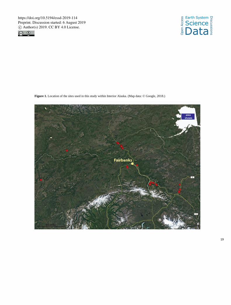
different soil properties from a large database (>3000 observations) of observations from Interior Alaska 52

(Figure 1). These properties were examined by degree of decomposition (via classification into distinct 53

organic soil horizons), soil drainage, and stand age. Our results can be used to: 1) gap fill when an 54

important soil property was not measured, 2) serve as baseline values to initialize boreal soil models, and 55

3) validate model results. 56

57

2 Methods 58

2.1 Field methodology 59

Soil cores were taken using one or more of four different methods. The first method, most often 60

used with surface layers, involved cutting soil blocks to a known volume. Another method often used to 61

sample these soils uses a coring device inserted into a hand drill (4.8 cm diameter; Nalder and Wein, 62

1998). Wetter sites were sometimes sampled while frozen using a Snow, Ice, and Permafrost Research 63

Establishment (SIPRE) corer (7.6-cm diameter; Rand and Mellor, 1985). Alternatively, if wetter sites 64

were sampled unfrozen we used a ‘frozen finger’. This coring method uses a thin-walled, hollow tube 65

(~6.5 cm diameter), sealed at one end, which is inserted into the ground until it hits mineral soil. A slurry 66

of dry ice and alcohol is then poured into the corer, freezing the unfrozen material surrounding the corer 67

to the outside. The corer is removed and the exterior of the core is scraped to remove any large roots or 68

material that stuck to the sample during removal. For some cores, two coring methods were combined to 69

create continuous samples from the surface to the mineral soil. 70

Cores were subdivided into subsections representing soil horizons based on visual factors such as 71

level of decomposition, color, and root abundance. These horizon samples provided the basis for our 72

analyses and are based on Canadian (Soil Classification Working Group, 1998) and U.S. Department of 73

Agriculture’s Natural Resource Conservation Service (Staff, 1998) soil survey techniques. A description 74

of the horizons and the codes we used to represent them are: 75

76


Ope

n A

cces

s Earth System

Science

DataD

iscussio

ns


5

77

Live moss

(L)

Live moss, which is usually green. This layer generally also contains a small amount of

plant litter.

Dead moss

(D)

Moss that is dead and either undecomposed or slightly decomposed. This horizon would

be considered an Oi horizon in the U.S. soil system.

Fibric

(F)

Fibrous plant material that varies in the degree of decomposition (somewhat intact to very

small plant pieces), but there is no amorphous organic material present. Very fine roots

often make up a large fraction of this horizon. This horizon would be considered an Oi

horizon in the U.S. soil system.

Mesic

(M)

This horizon is comprised of moderately decomposed material, with few, if any,

recognizable plant parts other than roots. There is amorphous present within this layer

to varying degrees, but it is not smeary. This horizon is generally considered an Oe

horizon (U.S. soil system).

Humic

(H)

This organic horizon is highly decomposed. The soil in this horizon smears when rubbed

and contains little to no recognizable plant parts. The H horizon is generally considered

an Oa horizon (U.S. soil system).

Mineral

(Min)

Classified as an A, B, or C mineral soil (U.S. soil system), it contains less than 20-volume-

percent organic matter, as judged in the field.

78

Because modeling so many different organic layers is difficult, we also combined layers as done in Yi 79

et al. (2009). The fibrous horizon combined the dead moss (D) and fibric (F) horizon, while the amorphous 80

horizon combined the mesic (M) and humic (H) horizon. These combinations were based on similarities in 81

decomposition state and depth. We also present data for several types of horizons that are only found at a 82

subset of sites: ash and burned organics are only found on the surface of recently burned sites, while lichen 83

and litter layers are only found on the surface of ~16 % of profiles. Our field studies also found several 84

horizon types (buried wood, grass, etc.) for which we did not have enough observations (5 or less). 85

We examined the effect of disturbance on soil properties by categorizing each of the soil profiles in 86

relation to time since the last disturbance, which we divided into three age classes: new (<5 yrs old), young 87

(5 – 50 yrs old), and mature (> 50 yrs old). All ‘new’ sites had recently burned and lost some portion of 88

their surface organic layers (Harden et al., 2000), which in turn effects soil moisture and temperature 89

(O'Donnell et al., 2010). Young sites had recently experienced fire or permafrost thaw. Both fire and thaw 90

change the dominant vegetation, thus influencing C inputs into the soil. They also influence soil temperature 91

and moisture, which in turn affects soil C stocks. 92


Ope

n A

cces

s Earth System

Science

DataD

iscussio

ns


6

Although classifications of soil drainage have been established for many soil types (Staff, 1993), the 93

presence of permafrost necessitates modifications of this system (Survey, 1982). Although generally 94

described (Harden et al., 2003; Johnstone et al., 2008), a soil drainage classification for permafrost 95

landscapes is lacking. Here we present such a classification, developed over the past two decades, for areas 96

of discontinuous permafrost (Figure 2). Well drained sites are similar to traditional drainage classifications, 97

in that water moves through the soil rapidly. However, moderately well drained drainage sites have 98

permafrost between 75 – 150 cm, which increases soil moisture of surface organics. Somewhat poorly, 99

poorly, and very poorly drained sites have some factor (permafrost, soil texture, or landscape position) that 100

inhibits drainage and causes redoximorephic features such as blue-grey colors in the mineral soil to appear. 101

Somewhat poorly drained sites have a shallow active layer (often around 50 cm), which affects soil moisture 102

and surface vegetation. Poorly drained sites experience saturated surface conditions only while seasonal ice 103

is present (usually May through early July). In contrast, very poorly drained sites have saturated surface 104

soils during the entire growing season. When sites are located on a slope >5 %, which helps promote 105

drainage (Woo, 1986; Carey and Woo, 1999), drainage class is increased by one step; we call this the 106

hillslope modifier. In addition, because burning increases active layer thickness, recently burned sites may 107

have deeper or no permafrost; therefore, we ascribed their soil drainage using nearby unburned sites. 108

109

2.2 Laboratory methodology 110

We air-dried soils at room temperature (20 °C to 30 °C) to constant mass, then oven-dried the 111

samples for 24-48 hours in a forced-draft oven. Organic soils were oven-dried at 65 °C to avoid the 112

alteration of organic matter chemistry. Mineral soils were oven-dried at 105 °C. Samples were then 113

processed in one of two ways, depending on the horizon code. Mineral soil samples were gently crushed 114

using a mortar and pestle, with care to break only aggregates, and then sieved through a 2-mm screen. Soil 115

particles that did not pass through the screen were removed, weighed, and saved separately; soil that passed 116

through the screen was then ground by using a mortar and pestle to pass through a 60-mesh (0.246-mm) 117

screen. The ground material was mixed and placed in a labeled glass sample bottle for subsequent analyses. 118


Ope

n A

cces

s Earth System

Science

DataD

iscussio

ns


7

Organic samples were weighed, and roots wider than 1 cm in diameter were removed, weighed, and saved 119

separately. The remaining sample material was then milled in an Udy Corp. Cyclone Sample Mill to pass 120

through a 0.25-mm screen and placed in a labeled glass vial. 121

We analyzed soil samples for total C and N using a Carlo Erba NA1500 elemental analyzer 122

(Fisons Instruments). In summary, samples were combusted in the presence of excess oxygen. The 123

resulting sample gases were carried by a continuous flow of helium through an oxidation furnace, 124

followed by a reduction furnace, to yield CO2, N2, and water vapor. Water was removed by a chemical 125

trap and CO2 and N2 were chromatographically separated before the quantification of C and N (Pella, 126

1990a,b). For organic horizon samples, where inorganic carbon (IC) is largely absent, total C represents 127

total organic C. For mineral-soil horizons were IC was present, we removed carbonates using the acid 128

fumigation technique (Komada et al., 2008) prior to running samples. Briefly, we preweighed samples in 129

silver capsules and transferred them to a small desiccator. Samples were wetted with 50 μL of deionized 130

water and then exposed to vaporous hydrochloric acid (1 N) for 6 hours, during which carbonates 131

degassed from samples as carbon dioxide. 132

133

2.3 Data quality and statistical methodology 134

Often the soil descriptions at the interface of the organic and mineral soil included notations 135

indicating that these horizons consisted of mixed organics and mineral soil. In the field the best call was 136

made to if it was mineral (<20 % C) or organic (≥20 % C). However, chemistry data often shows these 137

horizons were mislabeled (for example, a mineral soil with 22 % C). We used C chemistry to remove 138

organic soils with < 20 % C from our analyses. 139

All statistical analyses were run using the R program (Team, 2017). We first checked the data for 140

normality. Much of the data needed transformation (Table S1). The effects of drainage and age class, for 141

all soil horizons with the exception of the fibrous and amorphous horizons, was tested using the mixed-142

effects model command lmer (lme4; Bates et al., 2015), using profile (or soil core) as the random effect. 143

When significant, differences among drainage types or age class were determined using the difflsmeans 144


Ope

n A

cces

s Earth System

Science

DataD

iscussio

ns


8

command (lmerTest; Kuznetsova et al., 2017), which produces a Differences of Least Squares Means 145

table with p-values. For the evaluation of drainage and age class on thickness for the fibrous and 146

amorphous horizons, because all applicable samples within a soil profile were combined, we used an 147

analysis of variance model (aov) with the TukeyHSD function. 148

149

3. Dataset Review 150

3.1 Bulk density 151

Bulk density varied by depth and was significantly different (p < 0.05) among all horizon types 152

(live moss, dead moss, fibric, mesic, humic, and mineral soil; Table 1), including the two combined 153

horizon codes (fibrous and amorphous). Surprisingly, as they are comprised of very similar material, even 154

the live and dead moss layers had significantly different bulk densities. Bulk density increases ~10-fold 155

from one layer to the next as one progress down the soil profile (from 0.021 g/cm3 for live moss to 0.215 156

g/cm3 for humics). These differences are likely related to the length of time each soil layer has had to 157

decompose. As soil layers become older, plant fibers break down physically and biologically, becoming 158

smaller and more compressible. 159

Bulk density also varied by drainage class: well drained sites tended to have higher bulk densities 160

than other soil drainage classes (Table S1). While this pattern was not always significant it was consistent 161

for all horizons except for the dead moss horizon, where it was the 2nd highest. The higher bulk densities 162

of well-drained sites are likely related to two factors: 1) the influence of lichens and litters, which are 163

more often found within well drained sites and have higher bulk densities than moss (Table 3), and 2) the 164

influence of mineral soil, which, due to shallower organic soils, is more likely to be incorporated into 165

fibric (F) and mesic (M) horizons. This last reason is supported by the lower %C values also found within 166

well-drained F and M horizons (Table S2). New (< 5 yr old) sites tended to have slightly higher bulk 167

densities than the young and mature age classes (all horizons except for the humic horizon; Table S1). 168

However, the differences weren’t usually significant. 169

170


Ope

n A

cces

s Earth System

Science

DataD

iscussio

ns


9

3.2 Carbon 171

Upper soil layers (live moss, dead moss, and fibric horizons) are consistently higher in % C than 172

lower layers (mesic, humic, and mineral horizons; Table 1). Bulk density values also increase with depth 173

for these horizons, so that C storage values increase dramatically with depth (Figure 3). 174

C content varied by drainage class for the fibric and mesic layers (Table S3), which had lower % 175

C values in well drained as compared to more poorly drained sites. Lower C values for the fibric and 176

mesic well-drained sites are likely due to the inclusion of mineral soil material into these horizons, likely 177

due in large part to natural process such as cryoturbation or aeolian contributions. Somewhat poorly 178

drained sites also have lower C values for all organic soil horizons as compared to other non-well drained 179

classes. 180

C content increased with age class for the fibric and mesic horizons (Table S2). Since all sites 181

classified as ‘new’ were recently disturbed by fire, this increase could be due to both the inclusion of 182

more live roots and the loss of ash, which has a lower C content and is a component of recently burned 183

soil’s surface layers, within these two horizons as stands recover. 184

185

3.3 Nitrogen 186

All horizons had significantly different N concentrations from each other (Table 1). The amount 187

of N within the organic layers increased with depth. N was 2-3 times higher in the organic horizons as 188

compared to mineral soil. There was significant variability in N by drainage class for each horizon type 189

(Table S3). The poorly and very poorly drained sites had greater concentrations of N than then other 190

drainage classes for the fibric (F), mesic (M), and humic (H) horizons. These higher concentrations may 191

be due to the number of these observations (~40 %) from bogs and fens, which have been shown to have 192

higher litterfall N concentrations (Finger et al., 2016). There was also a trend of higher N in the new and 193

younger stands for the live and dead moss horizons (Table S3), which may be related to N quality of early 194

succession litterfall. 195

196


Ope

n A

cces

s Earth System

Science

DataD

iscussio

ns


10

3.4 C:N ratio 197

All horizon types had significantly different C:N ratio from one another (Table 4), with these 198

ratios tending to decrease as the horizons deepen and become more decomposed. There were no trends in 199

C:N ratio by drainage class. Age class played a role in C:N ratios for the less decomposed horizons, 200

where C:N ratio increase as stands aged. These trends are more influenced by changes in N by age class, 201

than changes in C. 202

203

3.5 Thickness 204

The factor that varied the most by horizon was the thickness of each horizon type (Table 1). 205

There was a very strong effect of drainage on thickness, with the well-drained sites having much thinner 206

soil horizons (and no humic horizon) than the other drainage classes and the very poorly drained sites 207

having much thicker soil horizons that the other drainage classes (Table 2). Age class also plays a role in 208

horizon thickness: new sites (<5 yrs old) had much thinner organic soil horizons than young or mature 209

sites (Table 3). Since new sites recently burned, these thin soil horizons are the result of the loss of 210

organics due to combustion. Both fire return interval and fire severity impact the amount of legacy soil 211

remaining (Harden et al., 2012), therefore fire history likely plays a large role in horizon thickness. 212

Vegetation could also influence horizon thickness. An examination of these data that included 213

current surface vegetation found greater thicknesses for sites with Sphagnum sp. and sedges, although this 214

factor usually wasn’t statistically significant. Historical vegetation could also influence horizon thickness. 215

For instance, if a site was Sphagnum dominated in the past, even if it’s not the current surface vegetation, 216

the soil profile is more likely to have thicker soil layers due to the slow decomposition rate of Sphagnum 217

(Turetsky et al., 2008). Because such historical factors are difficult to measure and predict, we 218

recommend that users of these data include the natural variability in thickness estimates in their analyses. 219

220

221


Ope

n A

cces

s Earth System

Science

DataD

iscussio

ns


11

3.6 How well do these values represent the data? 222

To test how well the values in Table 1 – 3 estimate C and N stocks we compared predicted versus 223

measured stocks for two locations. Our first test was for 142 samples taken from two chronosequences 224

(time since fire) located near Thompson, Manitoba (Manies et al., 2006). Each chronosequence represents 225

a different drainage class: moderately well drained versus somewhat poorly drained. These data were 226

taken using the same methods of sampling and describing soil horizons. We used the bulk density, C, and 227

N values based on horizon only (Table 1) and thickness based on horizon and drainage (Table 2). For 228

those profiles with high C or N stocks (> 5 gC/m2 and > 0.01 gN/m2, respectively) our predicted stocks 229

were consistently higher than measured stocks. This result is mostly due to greater predicted than 230

observed thicknesses, most dramatically for the mesic (M) horizons. In addition, our predicted bulk 231

density values tended to be slightly higher than measured values especially for the fibric (F) and humic 232

(H) horizons. We found that most the observations with large differences in predicted versus observed 233

stocks had anomalously low measured bulk densities. For example, there were some thick fibric horizons 234

with a bulk density of 0.01 g/cm2 (versus the predicted value of 0.06 g/cm2) and mesic horizons with a 235

bulk density of 0.05 g/cm2 (versus the predicted value of 0.15 g/cm2). These results could be because a) 236

our data, from Interior Alaska, does not well represent other black spruce, boreal regions, or b) our 237

average values, especially thickness, tend to overestimate stocks. 238

To determine if our previous results were due to regional differences, we also compared predicted 239

versus measured C stocks for a second study, this one located within Alaska (Kane and Ping, 2004). They 240

measured horizon thickness (all samples), C (all samples), and bulk density (one sample per site) for soil 241

profiles along a continuum of tree productivity. This work used the US Soil System to describe their soils, 242

dividing the organic horizons into Oi and Oe/Oa horizons. We chose to represent their Oi data, which they 243

described as slightly decomposed moss, with our dead moss (D) horizon and their Oe/Oa data, which they 244

described as intermediately decomposed moss with rare saprics, as our fibric (F) horizon. For this dataset 245

our predicted stocks were much less than measured stocks. This result is due to underestimating 246

thicknesses (both the Oi and Oe/Oa horizons) and bulk density (Oe/Oa horizon). The discrepancy in bulk 247


Ope

n A

cces

s Earth System

Science

DataD

iscussio

ns


12

density values may be because the bulk density samples taken by Kane and Ping (2004) were 5.08 cm in 248

diameter, while the actual thickness of these horizons they were measuring ranged between 1 and 25 cm. 249

Therefore, their measurements likely did not accurately characterize their soil horizons. These results also 250

point out potential issues that could arise with data described in a different manner (here the US Soil 251

System). While we made our best guess as to which of our horizons best fit their data, the measured Oe/Oa 252

bulk density ranged between 0.06 and 0.12 g/cm2, implying that their samples were likely a combination 253

of fibric (F) and mesic (M) horizons (which have average bulk densities of 0.07 and 0.15 g/cm2, 254

respectively, Table 1). 255

256

3.7 Caveats 257

It is important to include mineral soil in soil C stock evaluations, as the mineral soil of this region 258

contains large amounts of C, especially within Yedoma deposits (Hugelius et al., 2014; O'Donnell et al., 259

2011). However, the mineral soil data presented here do not represent full mineral soil profiles, since our 260

sampling often stopped 5-10 cm into mineral soil. Additional examinations into bulk density and C 261

concentrations of Alaskan mineral soil can be found in Ping et al. (2010), Michaelson et al. (2013), and 262

Ebel et al. (2019). 263

Our analysis includes Alaska data from >3,000 soil samples and >290 soil profiles, with samples 264

dominated by soil profiles from somewhat poorly, poorly, and very poorly drainages. Age classes were 265

also not equally distributed, as almost 50 % of our soil profiles were from mature stands. This unbalanced 266

design means that our results may not adequately represent all drainages and age classes, particularly 267

well-drained sites. Deciduous stands are not well represented. In addition, we have few sites from shrub 268

dominated ecosystems. Our data best represents black spruce dominated forests and thermokarst wetlands 269

in Alaska. 270

271

272


Ope

n A

cces

s Earth System

Science

DataD

iscussio

ns


13

4 Data Access 273

addition, many additional soil attributes, such as volumetric water content, von Post decomposition index, 275

and additional chemistry, can be found for the majority of these data through various USGS Open-File 276

Reports (Manies et al., 2017; Manies et al., 2016; Manies et al., 2014; O'Donnell et al., 2013; O'Donnell 277

et al., 2012; Manies et al., 2004). 278

279

5 Conclusions 280

Boreal ecosystems are especially sensitive and vulnerable due to climate change. Unfortunately, 281

most models do not do a good job recreating high latitude biogeochemical processes (Flato et al., 2013). 282

One reason for the discrepancies between model results and data is that many large scale models do a 283

poor job at recreating soil thermal dynamics, which is necessary for recreating permafrost dynamics 284

(Koven et al., 2013; Khvorostyanov et al., 2008). While these processes are starting to be incorporated 285

into land surface and regional models (see, for example, Genet et al., 2013; Koven et al., 2011), currently 286

few models include the “distinct properties of organic soils” that are found in the boreal region (Flato et 287

al., 2013). The data presented in this paper provide a needed dataset for initializing and validating models 288

related to boreal organic soils. In addition, these data can be used by scientists to gap-fill in instances 289

when an important soil property was not measured. 290

291

Acknowledgements 292

We would like to acknowledge the Bonanza Creek LTER and the USGS Fairbanks office for their support 293

of our work over the years. We would also like to thank the many people who assisted in collecting these 294

samples. This work, over the years, has been supported by the USGS (Land Resources, Climate and Land 295

Use Change, and Global Change programs), the National Science Foundation (DEB-0425328, EAR-296

0630249), and the NASA Terrestrial Ecology (NNX09AQ36G). 297

298

274 All data used in this manuscript is available from https://doi.org/10.5066/P960N1F9 (Manies, 2019). In


Ope

n A

cces

s Earth System

Science

DataD

iscussio

ns


14

Author contribution 299

KM prepared the manuscript with the help of MW and JH. All authors were involved in supporting the 300

collection of these data. 301

302

303


Ope

n A

cces

s Earth System

Science

DataD

iscussio

ns


15

References 304

Bates, D., Maechler, M., Bolker, B., and Walker, S.: Fitting Linear Mixed-Effects Models Using lme4, 305 Journal of Statistical Software, 67, 1-48, doi:10.18637/jss.v067.i01, 2015. 306

Bauer, I. E., Bhatti, J. S., Cash, K. J., Tarnocai, C., and Robinson, S. D.: Developing Statistical Models to 307 Estimate the Carbon Density of Organic Soils, Canadian Journal of Soil Science, 86, 295–304, 308 2006. 309

Bradshaw, C. J. A., and Warkentin, I. G.: Global estimates of boreal forest carbon stocks and flux, Global 310 and Planetary Change, 128, 24-30, https://doi.org/10.1016/j.gloplacha.2015.02.004, 2015. 311

Carey, S. K., and Woo, M. K.: Hydrology of two slopes in subarctic Yukon, Canada, Hydrological 312 Processes, 13, 2549-2562, 10.1002/(SICI)1099-1085(199911)13:16<2549::AID-313 HYP938>3.0.CO;2-H, 1999. 314

Deluca, T. H., and Boisvenue, C.: Boreal forest soil carbon: distribution, function and modelling, 315 Forestry: An International Journal of Forest Research, 85, 161-184, 10.1093/forestry/cps003, 316 2012. 317

Ebel, B. A., Koch, J. C., and Walvoord, M. A.: Soil Physical, Hydraulic, and Thermal Properties in 318 Interior Alaska, USA: Implications for Hydrologic Response to Thawing Permafrost Conditions, 319 Water Resources Research, 55, 4427-4447, 10.1029/2018wr023673, 2019. 320

Finger, R. A., Turetsky, M. R., Kielland, K., Ruess, R. W., Mack, M. C., and Euskirchen, E. S.: Effects of 321 permafrost thaw on nitrogen availability and plant–soil interactions in a boreal Alaskan lowland, 322 Journal of Ecology, 104, 1542-1554, 10.1111/1365-2745.12639, 2016. 323

Flato, G., Marotzke, J., Abiodun, B., Braconnot, P., Chou, S. C., Collins, W., Cox, P., Driouech, F., 324 Emori, S., Eyring, V., Forest, C., Gleckler, P., Guilyardi, E., Jakob, C., Kattsov, V., Reason, C., 325 and Rummukainen, M.: Evaluation of Climate Models, in: Climate Change 2013: The Physical 326 Science Basis. Contribution of Working Group I to the Fifth Assessment Report of the 327 Intergovernmental Panel on Climate Change, edited by: Stocker, T. F., Qin, D., Plattner, G.-K., 328 Tignor, M., Allen, S. K., Boschung, J., Nauels, A., Xia, Y., Bex, V., and Midgley, P. M., 329 Cambridge University Press, Cambridge, United Kingdom and New York, NY, USA, 741–866, 330 2013. 331

Genet, H., Mcguire, A. D., Barrett, K., Breen, A., Euskirchen, E. S., Johnstone, J. F., Kasischke, E. S., 332 Melvin, A. M., Bennett, A., Mack, M. C., Rupp, T. S., Schuur, A. E. G., Turetsky, M. R., and 333 Yuan, F.: Modeling the effects of fire severity and climate warming on active layer thickness and 334 soil carbon storage of black spruce forests across the landscape in interior Alaska, Environmental 335 Research Letters, 8, 45016-45016, 2013. 336

Harden, J. W., Trumbore, S. E., Stocks, B. J., Hirsch, A., Gower, S. T., O'neill, K. P., and Kaisischke, E. 337 S.: The role of fire in the boreal carbon budget, Global Change Biology, 6, S174–S184, 2000. 338

Harden, J. W., Meier, R., Silapaswan, C., Swanson, D. K., and Mcguire, A. D.: Soil drainage and its 339 potential for influencing wildfires in Alaska, in: Studies by the U.S. Geological Survey in Alaska, 340 2001, edited by: Galloway, J., U.S. Geological Survey Professional Paper 1678, 139–144, 2003. 341

Harden, J. W., Manies, K. L., O'donnell, J., Johnson, K., Frolking, S., and Fan, Z.: Spatiotemporal 342 analysis of black spruce forest soils and implications for the fate of C, Journal of Geophysical 343 Research, 117, G01012, 10.1029/2011JG001826, 2012. 344

Hugelius, G., Strauss, J., Zubrzycki, S., Harden, J. W., Schuur, E. a. G., Ping, C. L., Schirrmeister, L., 345 Grosse, G., Michaelson, G. J., Koven, C. D., O'donnell, J. A., Elberling, B., Mishra, U., Camill, 346 P., Yu, Z., Palmtag, J., and Kuhry, P.: Estimated stocks of circumpolar permafrost carbon with 347 quantified uncertainty ranges and identified data gaps, Biogeosciences, 11, 6573-6593, 348 10.5194/bg-11-6573-2014, 2014. 349

Jackson, R. B., Lajtha, K., Crow, S. E., Hugelius, G., Kramer, M. G., and Piñeiro, G.: The Ecology of 350 Soil Carbon: Pools, Vulnerabilities, and Biotic and Abiotic Controls, Annual Review of Ecology, 351 Evolution, and Systematics, 48, 419-445, 10.1146/annurev-ecolsys-112414-054234, 2017. 352


Ope

n A

cces

s Earth System

Science

DataD

iscussio

ns


16

353 Johnson, K. D., Harden, J. W., Mcguire, A. D., Bliss, N. B., Bockheim, J. G., Clark, M., Nettleton-

354 Hollingsworth, T., Jorgenson, M. T., Kane, E. S., Mack, M., O'donnell, J., Ping, C. L., Schuur, E.

355 a. G., Turetsky, M. R., and Valentine, D. W.: Soil carbon distribution in Alaska in relation to soil-

356 forming factors, Geoderma, 167-168, 10.1016/j.goederma.2011.10.006, 2011.

357 Johnstone, J. F., Hollingsworth, T. N., and Chapin, F. S., Iii: A key for predicting postfire successional

358 trajectories in black spruce stands of interior Alaska, USDA Forest Service, 37, 2008.

359 Johnstone, J. F., Hollingsworth, T. N., Chapin, F. S., Iii, and Mack, M. C.: Changes in fire regime break

360 the legacy lock on successional trajectories in Alaskan boreal forest, Global Change Biology, 16,

361 1281–1295, doi: 10.1111/j.1365-2486.2009.02051.x, 2010.

362 Jorgenson, M. T., Harden, J. W., Kanevskiy, M., O'donnell, J. A., Wickland, K. P., Ewing, S. A., Manies,

363 K. L., Zhuang, Q., Shur, Y., Striegl, R. G., and Koch, J. C.: Reorganization of vegetation,

364 hydrology, and soil carbon after permafrost degradation across heterogeneous boreal landscapes,

365 Environmental Research Letters, 8, 035017, 10.1088/1748-9326/8/3/035017, 2013.

366 Kane, E. S., and Ping, C.-L. L.: Soil carbon stabilization along productivity gradients in interior Alaska:

367 Summer 2003, Fairbanks, B. C. L.-U. o. A., http://www.lter.uaf.edu/data/data-detail/id/132,

368 BNZ:132, 2004, 10.6073/pasta/d09433eee2cb6587eca672864cf7e90f,

369 Khvorostyanov, D. V., Krinner, G., Ciais, P., Heimann, M., and Zimov, S. A.: Vulnerability of permafrost

370 carbon to global warming. Part I: model description and role of heat generated by organic matter

371 decomposition, Tellus B, 60, 250-264, 10.1111/j.1600-0889.2007.00333.x, 2008.

372 Komada, T., Anderson, M. R., and Dorfmeier, C. L.: Carbonate removal from coastal sediments for the

373 determination of organic carbon and its isotopic signatures, δ13C and Δ14C: comparison of

374 fumigation and direct acidification by hydrochloric acid, Limnology & Oceanography: Methods,

375 6, 254-262, 2008.

376 Koven, C. D., Ringeval, B., Friedlingstein, P., Ciais, P., Cadule, P., Khvorostyanov, D., Krinner, G., and

377 Tarnocai, C.: Permafrost carbon-climate feedbacks accelerate global warming, Proceedings of the

378 National Academy of Sciences, 108, 14769-14774, 10.1073/pnas.1103910108, 2011.

379 Koven, C. D., Riley, W. J., and Stern, A.: Analysis of permafrost thermal dynamics and response to

380 climate change in the CMIP5 Earth System Models, Journal of Climate, 26, 1877-1900, 2013.

381 Kuznetsova, A., Brockhoff, P. B., and Christensen, R. H. B.: lmerTest Package: Tests in Linear Mixed

382 Effects Models, Journal of Statistical Software, 82, 1-26, 10.18637/jss.v082.i13, 2017.

383 Manies, K.: Data Supporting Generalized models to estimate carbon and nitrogen stocks of organic layers

384 in Interior Alaska, 2019, US Geological Survey, https://doi.org/10.5066/P960N1F9, 2019. 385 Manies, K. L., Harden, J. W., Silva, S. R., Briggs, P. H., and Schmid, B. M.: Soil data from Picea

386 mariana stands near Delta Junction, Alaska of different ages and soil drainage types, U.S.

387 Geological Survey, Menlo Park, CA, Open File Report 2004-1271, 19, 2004.

388 Manies, K. L., Harden, J. W., and Veldhuis, H.: Soil data from a moderately well and somewhat poorly

389 drained fire chronosequence near Thompson, Manitoba, Canada, U.S. Geological Survey, Menlo

390 Park, CA, Open File Report 2006-1291, 17, 2006.

391 Manies, K. L., Harden, J. W., and Hollingsworth, T. N.: Soils, Vegetation, and Woody Debris Data from

392 the 2001 Survey Line Fire and a Comparable Unburned Site, US Geological Survey, 36, 2014.

393 Manies, K. L., Harden, J. W., Fuller, C. C., Xu, X., and Mcgeehin, J. P.: Soil Data for a Vegetation

394 Gradient Located at Bonanza Creek Long Term Ecological Research Site, Interior Alaska, US

395 Geological Survey, 20, 2016.

396 Manies, K. L., Fuller, C. C., Jones, M. C., Waldrop, M. P., and Mcgeehin, J. P.: Soil data for a

397 thermokarst bog and the surrounding permafrost plateau forest, located at Bonanza Creek Long

398 Term Ecological Research Site, Interior Alaska, Reston, VA, Report 2016-1173, 1-11, 2017.

399 Michaelson, G. J., Ping, C.-L., and Clark, M.: Soil Pedon Carbon and Nitrogen Data for Alaska: An

400 Analysis and Update, Open Journal of Soil Science, Vol.03No.02, 11, 10.4236/ojss.2013.32015,

401 2013.


Ope

n A

cces

s Earth System

Science

DataD

iscussio

ns


17

Mu, C., Zhang, T., Zhang, X., Li, L., Guo, H., Zhao, Q., Cao, L., Wu, Q., and Cheng, G.: Carbon loss and 402 chemical changes from permafrost collapse in the northern Tibetan Plateau, Journal of 403 Geophysical Research: Biogeosciences, 121, 1781-1791, 10.1002/2015JG003235, 2016. 404

Nalder, I. A., and Wein, R. W.: A new forest floor corer for rapid sampling, minimal disturbance and 405 adequate precision, Silva Fennica, 32, 373–381, 1998. 406

O'Donnell, J. A., Harden, J. W., Mcguire, A. D., and Romanovsky, V. E.: Exploring the sensitivity of soil 407 carbon dynamics to climate change, fire disturbance, and permafrost thaw in a black spruce 408 ecosystem, Biogeosciences, 7, 8853–8893, 10.5194/bgd-7-8853-2010, 2010. 409

O'Donnell, J. A., Harden, J. W., Mcguire, A. D., Kanevskiy, M. Z., and Jorgenson, M. T.: The effect of 410 fire and permafrost interactions on soil carbon accumulation in an upland black spruce ecosystem 411 of interior Alaska: Implications for post-thaw carbon loss, Global Change Biology, 1461–1474, 412 10.1111/j.1365-2486.2010.02358.x, 2011. 413

O'Donnell, J. A., Harden, J. W., Manies, K. L., and Jorgenson, M. T.: Soil data for a collapse-scar bog 414 chronosequence in Koyukuk Flats National Wildlife Refuge, Alaska, 2008., U.S. Geological 415 Survey, Open-File Report, 14, 2012. 416

O'Donnell, J. A., Harden, J. W., Manies, K. L., Jorgenson, M. T., Kanevskiy, M., and Xu, X.: Soil data 417 from fire and permafrost-thaw chronosequences in upland black spruce (Picea mariana) stands 418 near Hess Creek and Tok, Alaska, U.S. Geological Survey 16 p, 2013. 419

Osterkamp, T. E., Jorgenson, M. T., Schuur, E. a. G., Shur, Y. L., Kanevskiy, M. Z., Vogel, J. G., and 420 Tumskoy, V. E.: Physical and ecological changes associated with warming permafrost and 421 thermokarst in Interior Alaska, Permafrost and Periglacial Processes, 20, 235–256, 2009. 422

Ping, C., Boone, R. D., Clark, M. H., Packee, E. C., and Swanson, D. K.: State factor control of soil 423 formation in Interior Alaska, in: Alaska's changing boreal forest, edited by: Chapin Iii, F. S., 424 Oswood, M. W., Van Cleve, K., Viereck, L. A., and Verbyla, D. L., Oxford University Press, 425 Oxford, 21-38, 2006. 426

Ping, C. L., Michaelson, G. J., Kane, E. S., Packee, E. C., Stiles, C. A., Swanson, D. K., and Zaman, N. 427 D.: Carbon Stores and Biogeochemical Properties of Soils under Black Spruce Forest, Alaska, 428 Soil Science Society of America Journal, 74, 969–978, 2010. 429

Rand, J., and Mellor, M.: Ice-coring augers for shallow depth sampling, U.S. Army Cold Regions 430 Research and Engineering Laboratory, Hanover, New HampshireCRREL Report 85-21, 27, 1985. 431

Schadel, C., Bader, M. K. F., Schuur, E. a. G., Biasi, C., Bracho, R., Capek, P., De Baets, S., Diakova, K., 432 Ernakovich, J., Estop-Aragones, C., Graham, D. E., Hartley, I. P., Iversen, C. M., Kane, E., 433 Knoblauch, C., Lupascu, M., Martikainen, P. J., Natali, S. M., Norby, R. J., O/'Donnell, J. A., 434 Chowdhury, T. R., Santruckova, H., Shaver, G., Sloan, V. L., Treat, C. C., Turetsky, M. R., 435 Waldrop, M. P., and Wickland, K. P.: Potential carbon emissions dominated by carbon dioxide 436 from thawed permafrost soils, Nat. Clim. Chang., 6, 950-953, 10.1038/nclimate3054, 2016. 437

Schuur, E. A., Mcguire, A. D., Schädel, C., Grosse, G., Harden, J. W., Hayes, D. J., Hugelius, G., Koven, 438 C. D., Kuhry, P., Lawrence, D. M., Natali, S. M., Olefeldt, D., Romanovsky, V. E., Schaefer, K., 439 Turetsky, M. R., Treat, C. C., and Vonk, J. E.: Climate change and the permafrost carbon 440 feedback, Nature, 520, 171-179, 10.1038/nature14338, 2015. 441

Soil Classification Working Group: Canadian System of Soil Classification, 3rd ed., National Research 442 Council Canada Research Press, Ontario, 188 pp., 1998. 443

Staff, S. S.: Keys to soil taxonomy, 8th ed., Pocahontas Press, Blacksburg, Virginia, 599 pp., 1998. 444 Staff, S. S. D.: Examination and Description of Soil Profiles, in: Soil survey manual, edited by: Ditzler, 445

C., Scheffe, K., and Monger, H. C., USDA, Government Printing Office, Washington, D.C., 446 1993. 447

Survey, E. C. O. S.: The Canada Soil Information System (CanSIS): Manual for describing soils in the 448 field, LRRI Contribution No. 82-52, 175, 1982. 449

Turetsky, M. R., Crow, S. E., Evans, R. J., Vitt, D. H., and Wieder, R. K.: Trade-offs in resource 450 allocation among moss species control decomposition in boreal peatlands, Journal of Ecology, 96, 451 1297-1305, 10.1111/j.1365-2745.2008.01438.x, 2008. 452


Ope

n A

cces

s Earth System

Science

DataD

iscussio

ns


18

Turetsky, M. R., Kane, E. S., Harden, J. W., Ottmar, R. D., Manies, K. L., Hoy, E., and Kasichke, E. S.: 453 Recent acceleration of biomass burning and carbon losses in Alaskan forests and peatlands, 454 Nature Geosciences, 4, 27–31, 10.1038/NGEO1027, 2011. 455

Woo, M. K.: Permafrost hydrology in North America, Atmosphere-Ocean, 24, 201-234, 456 10.1080/07055900.1986.9649248, 1986. 457

Yi, S., Manies, K., Harden, J., and Mcguire, A. D.: Characteristics of organic soil in black spruce forests: 458 Implications for the application of land surface and ecosystem models in cold regions, 459 Geophysical Research Letters, 36, L05501, 10.1029/2008GL037014, 2009. 460

461

462


Ope

n A

cces

s Earth System

Science

DataD

iscussio

ns


19

Figure 1. Location of the sites used in this study within Interior Alaska. (Map data: © Google, 2018.)


Ope

n A

cces

s Earth System

Science

DataD

iscussio

ns


20

Figure 2. Soil drainage class decision tree.


Ope

n A

cces

s Earth System

Science

DataD

iscussio

ns


21

Figure 3. Trends in carbon and nitrogen storage (g/cm2) by horizon type using average values for bulk density, carbon, and nitrogen (see Table 1).

Horizon designations: L = live moss, D = dead moss, F = fibric, M = mesic, H = humic, Min = mineral.

0.0000

0.0005

0.0010

0.0015

0.0020

0.0025

0.0030

0.0035

0.0040

0.00

0.01

0.02

0.03

0.04

0.05

0.06

0.07

0.08

L D F M H Min

Nit

roge

n (

g/cm

2)

Car

bo

n (

g/cm

2)

Horizon type

SOC

SON


Ope

n A

cces

s Earth System

Science

DataD

iscussio

ns


22

Table 1. Bulk density (g/cm2), C (%), N (%), C:N ratio, and thickness (cm) for the main horizon codes.

Values in parenthesis are standard deviations. Significant differences (p < 0.05) among the main horizon

codes are indicated with different letters. There are no thickness values for mineral soil because these

results would reflect the thickness sampled, not the actual thickness of this horizon.

Horizon

Code

Bulk Density

(g/cm2)

Carbon

(%)

Nitrogen

(%)

C:N Thickness

(cm)

live moss

(L)

0.022a (0.018)

n=138

41.7a (3.8)

n=145

0.84a (0.25)

n=145

54a (16)

n=141

2.5a (1.6)

n=138

dead moss

(D)

0.039b (0.026)

n=540

42.6a (3.8)

n=538

0.77b (0.27)

n=537

62b (23)

n=541

14.3b (26.0)

n=161

fibrics

(F)

0.065c (0.041)

n=552

41.0a (5.6)

n=566

0.98c (0.42)

n=564

48c (17)

n=552

12.8c* (17.8)

n=225

mesics

(M)

0.149d (0.077)

n=634

38.2b (6.8)

n=650

1.42d (0.54)

n=651

31d (13)

n=634

20.4d* (40.3)

n=208

humics

(H)

0.215e (0.096)

n=160

32.1c (6.6)

n=164

1.53e (0.44)

n=164

22e (6)

n=160

10.0bc (11.5)

n=77

mineral

(Min)

0.731f (0.380)

n=584

6.5d (6.2)

n=674

0.34f (0.32)

n=673

18f (7)

n=603

n/a

fibrous

(D&F)

0.052 (0.037)

n=1092

41.8 (4.8)

n=1104

0.88 (0.37)

n=1101

29 (12)

n=794

22.8 (41.1)

n=220

amorphous

(M&H)

0.162 (0.085)

n=794

36.9 (7.2)

n=814

1.44 (0.52)

n=815

55 (21)

n=1093

19.7 (27.7)

n=263

*p-value very close to 0.05 (thickness F vs M = 0.044). These values are so close to our threshold of 0.05

we would like to recognize that there is a chance that the bulk density values are not significantly

different from each other.


Ope

n A

cces

s Earth System

Science

DataD

iscussio

ns


23

Table 2. Thickness (cm) of the main horizon codes by soil drainage and age class. The mineral soil horizon was not included in this table because

the way in which we sampled the mineral soil led to arbitrary thicknesses. Data presented are means, standard deviations (in parentheses), and

number of observations. Significant differences (p < 0.05) for horizon codes, among either drainage or age class, are indicated with different

letters.

Horizon Drainage Age class

Well-

drained

Moderately

well-drained

Somewhat

poorly

drained

Poorly

drained

Very poorly New Young Mature

live moss

(L)

2.2 (1.0)

n=6

2.5 (1.1)

n=13

2.1 (1.1)

n=75

1.5 (0.7)

n=18

4.3 (2.1)

n=26

1.0 (-) n=2

2.6 (2.1)

n=43

2.4 (1.2)

n=93

dead moss

(D)

3.3a (1.6)

n=20

8.1a (7.2)

n=20

7.5a (10.7)

n=78

6.5a (6.5)

n=21

38.8b (44.5)

n=36

6.3a (4.5)

n=17

16.4b (19.7)

n=45

14.7b (30.2)

n=99

fibrics

(F)

3.1a (3.0)

n=11

10.0abd (5.2)

n=18

8.0b (5.2)

n=123

13.6cd (11.0)

n=46

39.1bd (38.5)

n=27

6.6a (5.9)

n=65

19.1b (31.2)

n=41

14.0c (14.6)

n=119

mesics

(M)

2.8a (1.3)

n=5

12.4abc (16.7)

n=17

13.2b (37.9)

n=113

15.2c (23.0)

n=39

57.0d (53.8)

n=34

6.5ab (4.1)

n=54

20.9a (32.6)

n=53

27.6b (51.4)

n=101

humics

(H)

none 10.0ab (14.0)

n=9

6.2a (8.3)

n=38

7.4b (3.4)

n=13

20.7b (14.3)

n=17

4.3a (3.2)

n=24

13.4ab

(12.7) n=19

12.3b (13.2)

n=34

fibrous

(D&F)

4.5a (4.4)

n=12

15.5b (8.9)

n=22

11.6b (10.0)

n=136

14.6b (11.3)

n=52

59.8c (50.0)

n=41

7.3a (6.4)

n=73

26.7 (36.1)

n=47

23.5 (28.8)

n=133

amorphous

(M&H)

2.8a (1.3)

n=5

15.8a (24.5)

n=19

14.5a (38.3)

n=119

16.8a (22.3)

n=41

63.6b (51.5)

n=36

8.0 (5.3)a

n=57

23.5a (33.2)

n=58

30.5b (52.5)

n=105


Ope

n A

cces

s Earth System

Science

DataD

iscussio

ns


24

Table 3. Number of observations, bulk density (g/cm2), C (%), N (%), C:N ratio, and thickness (cm) of non-main horizon codes. Values in

parenthesis are standard deviations.

Horizon N Bulk density (g/cm2) Carbon (%) Nitrogen (%) C:N Thickness (cm)

ash 14 0.183 (0.155) 38.0 (14.4) 0.84 (0.34) 49 (20) 0.1 (-)

burned organics 99 0.122 (0.142) 38.6 (8.9) 1.07 (0.32) 99 (38) 1.6 (0.9)

lichen 31 0.034 (0.019) 40.3 (5.9) 0.76 (0.41) 69 (37) 3.6 (2.2)

litter 16 0.044 (0.018) 41.2 (3.1) 1.55 (0.52) 29 (10) 1.6 (0.9)


Ope

n A

cces

s Earth System

Science

DataD

iscussio

ns


Documents

Preprint - ESSD