Download pdf - Functions for Estimating Stem Diameter and Tree Age Using Tree Height, Crown Width and Existing Stand Database Information

227

Silva Fennica 39(2) research articles

Functions for Estimating Stem Diameter and Tree Age Using Tree Height, Crown Width and Existing Stand Database Information

Jouni Kalliovirta and Timo Tokola

Kalliovirta, J. & Tokola, T. 2005. Functions for estimating stem diameter and tree age using tree height, crown width and existing stand database information. Silva Fennica 39(2): 227–248.

The aim was to investigate the relations between diameter at breast height and maximum crown diameter, tree height and other possible independent variables available in stand databases. Altogether 76 models for estimating stem diameter at breast height and 60 models for tree age were formulated using height and maximum crown diameter as independent variables. These types of models can be utilized in modern remote sensing applications where tree crown dimensions and tree height are measured automatically. Data from Finnish national forest inventory sample plots located throughout the country were used to develop the models, and a separate test site was used to evaluate them. The RMSEs of the diameter models for the entire country varied between 7.3% and 14.9% from the mean diameter depending on the combination of independent variables and spe-cies. The RMSEs of the age models for entire country ranged from 9.2% to 12.8% from the mean age. The regional models were formulated from a data set in which the country was divided into four geographical areas. These regional models reduced local error and gave better results than the general models.

The standard deviation of the dbh estimate for the separate test site was almost 5 cm when maximum crown width alone was the independent variable. The deviation was smallest for birch. When tree height was the only independent variable, the standard devia-tion was about 3 cm, and when both height and maximum crown width were included it was under 3 cm. In the latter case, the deviation was equally small (11%) for birch and Norway spruce and greatest (13%) for Scots pine.

Keywords forest inventory, crown diameter, stem diameter, modelingAuthors´ address University of Helsinki, Dept. of Forest Resource Management, P.O.Box 27, FI-00014 University of Helsinki, FinlandE-mail [email protected] 27 September 2004 Revised 17 February 2005 Accepted 18 May 2005

228


1 Introduction

The development of modern remote sensing sen-sors has increased the need to create new forest models (Maltamo et al. 2003). One of the most promising methods is to use high resolution digi-tal aerial photographs (Pollock 1996, Gong et al. 2002, Korpela 2004, Wang et al. 2004) or laser scanning (Hyyppä et al. 2001, Holmgren 2003, Næsset 2004) to measure individual trees. As early as the 1970s, Jakobsons (1970) and Talts (1977) described the possibility of measuring the height of a tree, the crown diameter or even the diameter at breast height on aerial photographs by photogrammetry. However, these measure-ments usually only represent the dimensions of the crown as visible on the aerial photographs, the resolution and visibility of small branches and irregular crown parameters being dependent on the scale of the photograph. In theory, however, a close correlation exists in principle between crown diameter and stem characteristics, such as diameter at breast height, and the latter is also highly correlated with the photogrammetrically measured crown diameter, a relation for which Petlewitz (1976) observed a correlation coef-ficient of 0.9 in Pinus silvestris and a standard deviation of the regression of 2.5 cm. Klier (1970) emphasized the influence of scale, image quality, species and species mixture, while the close rela-tionship between these variables motivated many researchers (e.g. Sayn-Wittenstein et al. 1967) to construct aerial tree and stand volume tables based on crown diameter. Such tables, based on stand height, crown closure and crown diameter as independent variables or in a modified form (Eid and Næsset 1998, Gingrich et al. 1955, Avery and Meyer 1959), are today in common use in North America and Norway.

Krajicek et al. (1961) studied relations of crown and diameter at breast height in open-grown trees not confounded by competition, measuring 340 such trees in eastern Iowa. The crown width of a tree in an open stand is closely related to its diameter at breast height, the correlation coeffi-cient for every species being over 0.98. This rela-tion was found to be independent of age and site quality, but differed slightly between tree species. Open-grown trees were shorter than forest-grown

ones of the same diameter on similar soils and under similar conditions. This is attributed to competition between adjacent trees under forest conditions, a factor which also tends to reduce the size of the live crown, and especially the crown width.

Ilvessalo (1950) and Jakobsons (1970) studied the correlation between tree crown diameter and diameter at breast height under boreal managed forest conditions. Ilvessalo (1950) found that as branches are cloaked by adjacent trees, measure-ments of maximum crown diameter on photo-graphs are generally smaller than those made on the ground. Also, crown diameter varies with tree species, tree height, site and stand density. The correlation between crown diameter and diameter at breast height was best for Scots pine and much weaker for Norway spruce. Jakobsons (1970) studied this correlation for pine, spruce and birch separately and reached the following conclusions for trees belonging to the same diameter (at breast height) class. Conifers have smaller crown diam-eters than deciduous trees, but the location of the tree is also important, such that trees in southern Sweden have greater crown diameters than those in the north. Meanwhile, trees on poor sites or in open stands have greater crown diameters than those on nutrient-rich sites or in denser stands. Jakobsons (1970) also found that an almost linear relation exists between crown diameter and diameter at breast height, although this differed between tree species and between geographically distant trees. The crown diameter of young trees was wider than that of older trees. The relation was also confounded by competition between trees, the availability of light and site factors. Jakobsons (1970) nevertheless maintained that it was possible to estimate diameter at breast height as a function of crown diameter. Talts (1977), by contrast, concluded that also other independent variables in addition to crown diameter were necessary.

Nash (1949) and Nyyssönen (1955) found a standard error of 0.6 m in crown diameter esti-mates on photographs, and Worley et al. (1955) obtained a standard error between 0.9 m and 1.2 m on 1:12 000 photographs. More recently, Hilde-brandt (1996) reconstructed the dbh distribution of beech stands from the observed distribution of crown widths. Stand age can also be estimated

229

Kalliovirta and Tokola Functions for Estimating Stem Diameter and Tree Age Using Tree Height, Crown Width and …

from a regression equation with photogrammetri-cally determined stand height and crown size as the predictor variables, although because of the inherent uncertainties, a given stand is usually assigned to one of 20 year classes. Studies in Germany (see Van Laar and Akca 1997) have indicated that the age class of a stand can be esti-mated from photographic measurements.

New measuring methods, such as laserscanning (Hyyppä et al. 2001, Holmgren 2003, Næsset 2004) or digital photogrammetry (Korpela 2000, 2004); have specific characteristics and measure-ment techniques. Because imaging condition and applicability of tree measurements differ accord-ing to the distance to objects, the relative position of the tree and other similar factors, traditional photography-based crown diameter measure-ments are not a good basis for modelling. When allometric tree models are created using field measurement, separate calibration models can be used to relate photography-based measurements and ground measurements with improved accu-racy. When models are applied directly without calibration using automatic segmentation, small trees are easily overestimated and large trees are underestimated (Ikonen 2004). This type of error can be reduced using calibration techniques which utilize imaging parameters and few field observations (Mäkinen 2004). The models can be directly applied, when laser scanning is used as a remote sensing technique. Tree volume can then be derived from these variables using a chain of models in which diameter at breast height is estimated first. The aim of this study was to inves-tigate the relations between diameter at breast height and maximum crown diameter, tree height and other possible independent variables and to formulate models for estimating the diameter at breast height using different independent vari-ables and chains of models. Models for tree age were also formulated, with height and maximum crown diameter as independent variables.

2 Material

The main material used in the present work was based on the 1889 permanent sample plots estab-lished throughout Finland for the purposes of the

Finnish National Forest Inventory (NFI). Plot size varied according to diameter at breast height of a tree. Plot size was 100 m2, when diameter was under 10.5 cm and otherwise 300 m2. An addi-tional data set (Korpela 2004), comprising 346 Scots pines, 245 Norway spruces and 120 birches on a site near the Hyytiälä Research Station, was used to validate the models.

The NFI sample plot network is based on clus-ter sampling, where each cluster in southern Fin-land includes four sample plots and each cluster in northern Finland three. The distance between two clusters is also greater in the north than in the south, as is the sample plot interval. The mate-rial contains data from the 1st and 3rd rounds of measurements made on the permanent sample plots (in 1985–86 and 1995).

The material includes only trees for which crown diameter measurements are available, and only the data for 1995 were used to formulate the models. The crown diameters in the NFI material were measured according to field instructions, i.e. by taking the widest dimension of the crown. Any obvious mistakes in measuring and recording the data were removed, leaving a total set of 11 246 trees. Trees have been classified according to their position in the stand into the following categories: dominant (63%), intermediate (33%), and suppressed (4%), which refer to determined relative height of tree, over 80 %, 50–80% and less than 50%, respectively. The locations of the clusters are presented in Fig. 1.

The material also includes damaged and dis-eased trees, which can exhibit a highly abnormal relation between diameter at breast height and either height or crown diameter, causing bias in the models. It is assumed that living trees can be identified by remote sensing material. This may not be the case if the top of the tree is broken or the tree is dying (barely any living canopy left). After removing these abnormal trees, the data used for the diameter at breast height and the age models comprised 5303 Scots pines, 3661 Norway spruces and 2282 birches. The average values for the sample tree and stand variables are presented in Table 1. A caliper was used to measure the diameter at breast height, a Suunto hypsometer to measure tree height, an increment borer to measure tree age and a Kajanus tube to measure crown width.

230


Fig. 1. Models were constructed for all of Finland (right side) and for four separate regions (left side). Geographical regions are defined by the forest flora and climatic conditions (1 = Hemiboreal, 2 = South boreal, 3 = Middle boreal, 4 = North boreal). The entire area is covered by clusters. The locations of the clusters are shown on the right side of the figure.

As the relations between tree variables may vary depending on the location (see Jakobsons 1970), the material for the entire country was divided into four geographical areas defined according to the forest flora and climatic condi-tions (Fig. 1). The resulting distribution is pre-sented in Table 2.

3 Methods

Due to the hierarchical nature of the data, a mixed effect method with iterative general-ized least squares (IGLS) was used for linear-ized regression. The independent variables were selected according to the requirements defined for the new forest inventory procedure, i.e. that all independent variables should be accessible from high resolution aerial photographs or existing databases. The photogrammetric variables were height, maximum crown diameter, stem number of dominant trees per hectare and relative tree

height class. The photogrammetric variables and variables from the stand database were treated as independent variables in the regression model. The intercept was the only fixed effect of the basic model. Clusters and plots were treated as random effects. The form of model is

y = Xb + Zc + e ⇔ ykji = xkji´b + ck +dkj+ ekji,

where y is an n × 1 vector of observed values of the dependent variable, b is a p × 1 vector of fixed parameters, X is an n × p matrix of independent variables associated with fixed parameters, c is a q × 1 vector of random parameters with expecta-tion zero, Z is an n × q matrix of explanatory variables associated with random parameters and e is an n × 1 vector of error terms, e ~ N(0,σ2). Furthermore, in this case, k is the cluster to which the tree i in the plot j belongs, ck is the random parameters of cluster k and dkj is the random parameters of plot j.

The variables (α) from existing stand databases

231


that were tested were similar to variables which can be found in the forest planning databases provided by private forest owners in Finland, together with a few generally accepted variables: x co-ordinate, y co-ordinate, height above sea level, temperature sum, mean diameter, mean age, tree class, basal area, land-use class, site class and

soil type. Stand variables, which could be derived from an aerial photograph, such as stem number of dominant trees per hectare and relative tree height, were also tested. In general, dominant height is defined as the mean height of the 100 thickest trees at breast height in one hectare. In the context of this study only tree heights can be used to define dominant height because diameters are not known. Dominant tree is defined as a tree which height is more than 80 % from dominant height. Relative tree height could be estimated by comparing the height of the recognized tree to the dominant height of the recognized trees of the remote sensing material on a site. Relative tree height class is used as a dummy variable (D9). It indicates that a tree is suppressed or dominated defined as a tree which height is under 80 percent

Table 1. Mean statistics of field material (NFI) by species.

N Mean Sd Min Max

D1,3, mm Pine 5303 145 69 4 574 Spruce 3661 148 78 4 515 Birch 2282 115 56 6 532

H, dm Pine 5303 113 47 14 286 Spruce 3661 123 59 14 318 Birch 2282 113 44 16 310

Dcrm, dm* Pine 5303 31 12 4 101 Spruce 3661 33 12 6 95 Birch 2282 33 12 7 104

Age, years Pine 5303 59 34 11 297 Spruce 3661 66 31 12 278 Birch 2282 48 20 3 148

x, km 11246 3452 122 3117 3725y, km 11246 7015 208 6650 7725Altitude (alt), m 11246 127 65 0 410Temperature sum (ts), ° 11246 1100 164 531 1425Basal area (ba), m2/ha 11246 20.9 7.9 1 48Mean diameter (d1,3m), cm 11246 17.4 6.5 6 46Mean age (agem), years 11246 71.9 40.3 12 334Number of trees/ha (n) 11246 1554 934 33 7067Relative tree height class (dummy) 11246 0 1Site class (dummy) 11246 0 1Soil type (dummy) 11246 0 1Land-use class (dummy) 11246 0 1

* Dcrm refers to maximum crown diameter

Table 2. Number of trees of NFI field plots in different geographical areas.

Pine Spruce Birch Total

Area 1 129 104 39 272Area 2 1840 2180 871 4891Area 3 2641 1200 1190 5031Area 4 693 177 182 1052

232


from dominant height, therefore differing from a dominant or emergent tree. A model with three variables (h, dcrm, α) was chosen for each tree spe-cies and area based on a log likelihood ratio test (Goldstein 1995) achieving the best coefficient of determination.

To meet the normality and homoscedaticity assumptions, square root and logarithm trans-formations were used for the independent and dependent variables.

The models for diameter at breast height were of the forms:

d f h1 3, = ( ) + ε (1)

d f dcrm1 3, = ( ) + ε (2)

d f h dcrm1 3, ,= ( ) + ε (3)

d f h dcrm1 3, , ,= ( ) +α ε (4)

and the age models of the forms:

ln( ) ln( )age f h= ( ) + ε (5)

ln( ) ln( )age f dcrm= ( ) + ε (6)

ln( ) ln( ),ln( )age f h dcrm= ( ) + ε (7)

whered1,3 = diameter at breast height (mm),h = height (dm),dcrm = crown diameter, maximum (dm)α = stand variable from database or aerial

photograph

The models were used to estimate the value of the variable in its original unit of measurement. As non-linear transformations were used for the dependent variables, such an estimate will be biased (Lappi 1993), an effect that can be reduced by bias correction. Taking this into account, the model for diameter at breast height assumes the form

d f1 32

, var( )= ( ) + ε

and the age model the form

age f= ( ) ∗ +

exp var( )11

2ε

R2 was calculated separately to cluster, plot and tree effects, e.g. R2 for plot indicates the propor-tion of variance between plots, that is explained by a model. Proportion of total variance between clusters and between plots are also presented. R2 was calculated using a method described in Lappi (1997), where relation of estimated full mixed model variance and initial variance of random effect model of clusters and plots (the fixed part includes only a constant) were utilized as follows:

R(estimated variance of full model)

(ini2 1= −

ttial variance of model)

The non-linear extra sum of squares method (Bates and Watts 1988) was used to evaluate the differences between the geographical areas. The method requires the fitting of full and reduced models. The full model corresponds to different sets of parameters for each of the geographical areas involved. The reduced model corresponds to the same set of parameters for all regions. The suitability of the division and the need for any division at all were assessed on the basis of the test results. The appropriate test statistic is described in Bates and Watts (1988).

4 Results

4.1 Data Analysis for Modelling

The normality and homoscedasticity of models were tested. As an example of a model that meets these assumptions well, the diameter of Scots pines at breast height in area 3 is presented in Fig. 2. There were about 2640 pines in the area.

Altogether 136 models were constructed. These were numbered using a system in which the first digit for a model defines the geographic area (Fig. 1) in question (number of the area or 9 as an indication of the entire country), the second digit the form of the model and the last the tree species. For example, model 2.2.3 applies to diameter

233


model for birch in area 2 (tree species = 3), with the maximum diameter of the crown as the only independent variable (form of the model = 2). It should be noted that tree height and maximum crown diameter are expressed in decimetres in all the models, yielding the diameter at breast height in millimetres.

4.2 Models for Diameter at Breast Height

The data for all sample plots in the country were used to formulate the first set of models for

diameter at breast height. General information on these models is given by tree species in Table 3. As it can be seen, even the best third independ-ent variable, y co-ordinate for Scots pine and temperature sum for Norway spruce and birch, was of minor significance. The models for the diameter at breast height for the entire country are presented in Table 4.

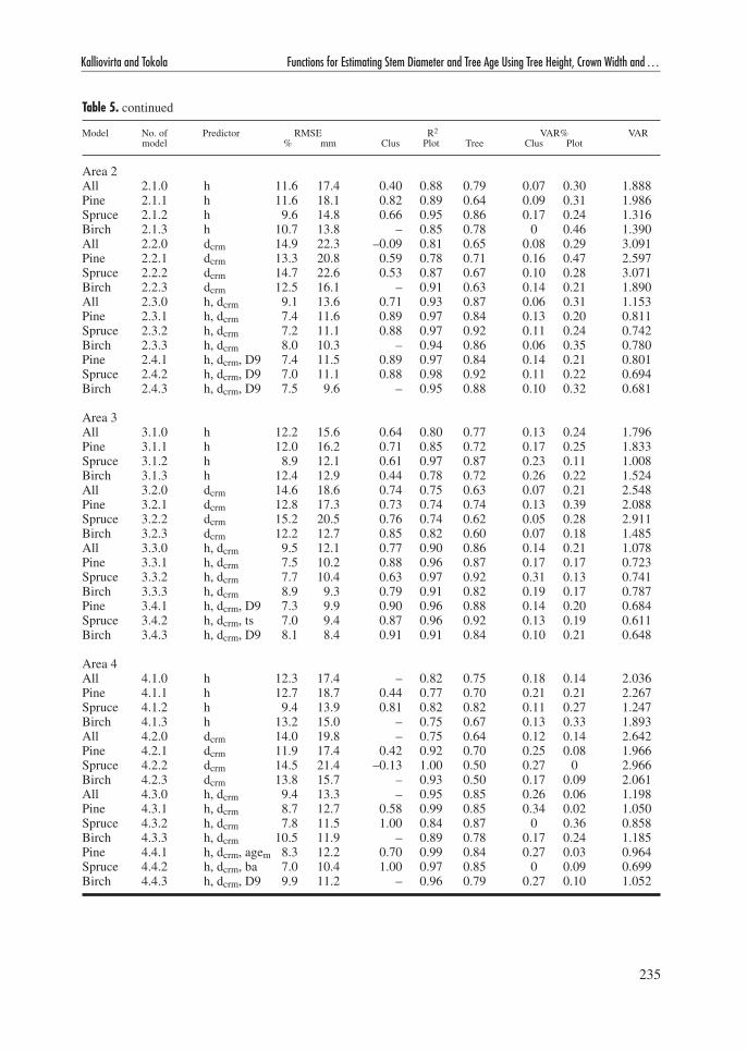
Further models for diameter at breast height were formulated after dividing the data into four geographical areas. General information on these regional models is presented in Table 5. The RMSEs of the models for the ecoregions varied

��

��

��

��

�

�

�

�

�

� ��

��

�

��

��

��

��

��

��

��

Fig. 2. Diagnostic testing of the model d1,3 = f(h, dcrm) for Scots pine in area 3. Residual plot in the left side and normality plot of residuals in the right side.

Table 3. Statistical properties of the models for the entire country. R2 is divided into cluster (Clus), plot (Plot) and tree (Tree) effects. Proportion of total variance (VAR%) is calculated for clusters and plots. The first digit in number of model refers to the geographic area (Fig. 1) in question (number of the area or 9 as an indication of the entire country), the second digit the form of the model and the last digit the tree species.

Model No. of Predictor RMSE R2 VAR% VAR model % mm Clus Plot Tree Clus Plot

All 9.1.0 h 12.5 17.5 0.53 0.85 0.77 0.18 0.23 2.058Pine 9.1.1 h 12.3 17.8 0.76 0.85 0.68 0.18 0.26 2.057Spruce 9.1.2 h 10.1 15.0 0.24 0.94 0.86 0.26 0.23 1.408Birch 9.1.3 h 13.1 15.0 0.31 0.83 0.73 0.30 0.26 1.854All 9.2.0 dcrm 14.8 20.7 0.70 0.78 0.64 0.08 0.25 2.862Pine 9.2.1 dcrm 13.0 18.8 0.75 0.75 0.72 0.16 0.39 2.309Spruce 9.2.2 dcrm 14.9 22.1 0.39 0.84 0.63 0.10 0.28 3.056Birch 9.2.3 dcrm 12.8 14.7 0.72 0.88 0.60 0.13 0.19 1.770All 9.3.0 h, dcrm 9.8 13.8 0.67 0.91 0.86 0.21 0.22 1.269Pine 9.3.1 h, dcrm 8.0 11.6 0.87 0.96 0.85 0.23 0.16 0.869Spruce 9.3.2 h, dcrm 8.3 12.3 0.38 0.96 0.91 0.32 0.21 0.948Birch 9.3.3 h, dcrm 9.6 11.0 0.65 0.93 0.82 0.28 0.19 1.000All 9.4.0 h, dcrm, D9 9.3 13.0 0.73 0.92 0.87 0.19 0.21 1.141Pine 9.4.1 h, dcrm, y 7.7 11.1 0.91 0.96 0.86 0.17 0.17 0.806Spruce 9.4.2 h, dcrm, ts 7.3 10.8 0.80 0.96 0.91 0.13 0.26 0.738Birch 9.4.3 h, dcrm, ts 8.8 10.1 0.84 0.92 0.84 0.16 0.25 0.838

234


Table 4. Parameter estimates and t-test statistics (t) of models for diameter at breast height for the entire country. The first digit in number of model refers to the geographic area (Fig. 1) in question (number of the area or 9 as an indication of the entire country), the second digit the form of the model and the last digit the tree species.

No. of Constant H Dcrm D9,ts or ymodel Estimate t Estimate t Estimate t Estimate t

9.1.0 –0.905 –13.92 1.176 196.00 – – – –9.1.1 –0.801 –7.63 1.204 120.40 – – – –9.1.2 –0.524 –6.39 1.145 163.57 – – – –9.1.3 –1.591 –9.94 1.153 76.87 – – – –9.2.0 –1.525 –17.33 – – 2.334 155.60 – –9.2.1 –0.238 –2.27 – – 2.183 121.28 – –9.2.2 –3.600 –21.30 – – 2.719 93.76 – –9.2.3 –0.982 –6.25 – – 2.019 74.78 – –9.3.0 –3.424 –58.03 0.806 134.33 1.148 82.00 – –9.3.1 –3.155 –42.64 0.730 91.25 1.323 82.69 – –9.3.2 –3.214 –35.71 0.861 95.67 1.016 44.17 – –9.3.3 –3.341 –26.31 0.700 46.67 1.143 42.33 – –9.4.0 –1.907 –26.49 0.733 122.17 1.066 82.00 –0.771 –33.529.4.1 –11.934 –22.20 0.752 91.48 1.311 84.62 0.00122 17.439.4.2 0,088 0.58 0.876 107.07 1.033 47.74 –0.00312 –26.009.4.3 –0.656 –3.59 0.805 52.08 1.056 40.64 –0.00302 –18.88

Table 5. Statistical properties of regional models. R2 is divided into cluster (Clus), plot (Plot) and tree (Tree) effects. Proportion of total variance (VAR%) is calculated for clusters and plots. The first digit in number of model refers to the geographic area (Fig. 1) in question (number of the area or 9 as an indication of the entire country), the second digit the form of the model and the last digit the tree species.


Area 1All 1.1.0 h 12.0 20.6 0.63 0.84 0.70 0.12 0.31 2.336Pine 1.1.1 h 10.3 18.7 – 0.86 0.56 0 0.40 1.839Spruce 1.1.2 h 11.2 18.5 – 0.93 0.77 0.29 0.20 1.940Birch 1.1.3 h 12.5 18.8 – 0.86 0.76 0 0.82 2.140All 1.2.0 dcrm 13.7 23.4 0.79 0.70 0.67 0.05 0.45 3.018Pine 1.2.1 dcrm 12.8 23.2 – 0.68 0.56 0 0.61 2.844Spruce 1.2.2 dcrm 12.5 20.6 – 0.82 0.66 0 0.40 2.418Birch 1.2.3 dcrm 15.1 22.7 – 0.79 0.61 – 0.80 3.144All 1.3.0 h, dcrm 8.7 15.0 0.81 0.90 0.86 0.11 0.37 1.237Pine 1.3.1 h, dcrm 7.6 13.8 – 0.93 0.75 0 0.39 1.011Spruce 1.3.2 h, dcrm 7.2 11.9 – 0.96 0.90 0.19 0.25 0.801Birch 1.3.3 h, dcrm 8.6 12.9 – 0.96 0.67 0 0.48 1.019Pine 1.4.1 h, dcrm, agem 7.1 12.9 – 0.95 0.75 0 0.29 0.875Spruce 1.4.2 h, dcrm, ba 6.7 11.1 – 0.97 0.90 0.14 0.22 0.702Birch 1.4.3 h, dcrm, d1,3m 8.5 12.7 – 0.95 0.76 0 0.61 0.986

235


Table 5. continued


Area 2All 2.1.0 h 11.6 17.4 0.40 0.88 0.79 0.07 0.30 1.888Pine 2.1.1 h 11.6 18.1 0.82 0.89 0.64 0.09 0.31 1.986Spruce 2.1.2 h 9.6 14.8 0.66 0.95 0.86 0.17 0.24 1.316Birch 2.1.3 h 10.7 13.8 – 0.85 0.78 0 0.46 1.390All 2.2.0 dcrm 14.9 22.3 –0.09 0.81 0.65 0.08 0.29 3.091Pine 2.2.1 dcrm 13.3 20.8 0.59 0.78 0.71 0.16 0.47 2.597Spruce 2.2.2 dcrm 14.7 22.6 0.53 0.87 0.67 0.10 0.28 3.071Birch 2.2.3 dcrm 12.5 16.1 – 0.91 0.63 0.14 0.21 1.890All 2.3.0 h, dcrm 9.1 13.6 0.71 0.93 0.87 0.06 0.31 1.153Pine 2.3.1 h, dcrm 7.4 11.6 0.89 0.97 0.84 0.13 0.20 0.811Spruce 2.3.2 h, dcrm 7.2 11.1 0.88 0.97 0.92 0.11 0.24 0.742Birch 2.3.3 h, dcrm 8.0 10.3 – 0.94 0.86 0.06 0.35 0.780Pine 2.4.1 h, dcrm, D9 7.4 11.5 0.89 0.97 0.84 0.14 0.21 0.801Spruce 2.4.2 h, dcrm, D9 7.0 11.1 0.88 0.98 0.92 0.11 0.22 0.694Birch 2.4.3 h, dcrm, D9 7.5 9.6 – 0.95 0.88 0.10 0.32 0.681

Area 3All 3.1.0 h 12.2 15.6 0.64 0.80 0.77 0.13 0.24 1.796Pine 3.1.1 h 12.0 16.2 0.71 0.85 0.72 0.17 0.25 1.833Spruce 3.1.2 h 8.9 12.1 0.61 0.97 0.87 0.23 0.11 1.008Birch 3.1.3 h 12.4 12.9 0.44 0.78 0.72 0.26 0.22 1.524All 3.2.0 dcrm 14.6 18.6 0.74 0.75 0.63 0.07 0.21 2.548Pine 3.2.1 dcrm 12.8 17.3 0.73 0.74 0.74 0.13 0.39 2.088Spruce 3.2.2 dcrm 15.2 20.5 0.76 0.74 0.62 0.05 0.28 2.911Birch 3.2.3 dcrm 12.2 12.7 0.85 0.82 0.60 0.07 0.18 1.485All 3.3.0 h, dcrm 9.5 12.1 0.77 0.90 0.86 0.14 0.21 1.078Pine 3.3.1 h, dcrm 7.5 10.2 0.88 0.96 0.87 0.17 0.17 0.723Spruce 3.3.2 h, dcrm 7.7 10.4 0.63 0.97 0.92 0.31 0.13 0.741Birch 3.3.3 h, dcrm 8.9 9.3 0.79 0.91 0.82 0.19 0.17 0.787Pine 3.4.1 h, dcrm, D9 7.3 9.9 0.90 0.96 0.88 0.14 0.20 0.684Spruce 3.4.2 h, dcrm, ts 7.0 9.4 0.87 0.96 0.92 0.13 0.19 0.611Birch 3.4.3 h, dcrm, D9 8.1 8.4 0.91 0.91 0.84 0.10 0.21 0.648

Area 4All 4.1.0 h 12.3 17.4 – 0.82 0.75 0.18 0.14 2.036Pine 4.1.1 h 12.7 18.7 0.44 0.77 0.70 0.21 0.21 2.267Spruce 4.1.2 h 9.4 13.9 0.81 0.82 0.82 0.11 0.27 1.247Birch 4.1.3 h 13.2 15.0 – 0.75 0.67 0.13 0.33 1.893All 4.2.0 dcrm 14.0 19.8 – 0.75 0.64 0.12 0.14 2.642Pine 4.2.1 dcrm 11.9 17.4 0.42 0.92 0.70 0.25 0.08 1.966Spruce 4.2.2 dcrm 14.5 21.4 –0.13 1.00 0.50 0.27 0 2.966Birch 4.2.3 dcrm 13.8 15.7 – 0.93 0.50 0.17 0.09 2.061All 4.3.0 h, dcrm 9.4 13.3 – 0.95 0.85 0.26 0.06 1.198Pine 4.3.1 h, dcrm 8.7 12.7 0.58 0.99 0.85 0.34 0.02 1.050Spruce 4.3.2 h, dcrm 7.8 11.5 1.00 0.84 0.87 0 0.36 0.858Birch 4.3.3 h, dcrm 10.5 11.9 – 0.89 0.78 0.17 0.24 1.185Pine 4.4.1 h, dcrm, agem 8.3 12.2 0.70 0.99 0.84 0.27 0.03 0.964Spruce 4.4.2 h, dcrm, ba 7.0 10.4 1.00 0.97 0.85 0 0.09 0.699Birch 4.4.3 h, dcrm, D9 9.9 11.2 – 0.96 0.79 0.27 0.10 1.052

236


Table 6. Parameter estimates and t-test statistics (t) of regional models for diameter at breast height. The first digit in number of model refers to the geographic area (Fig. 1) in question (number of the area or 9 as an indication of the entire country), the second digit the form of the model and the last digit the tree species.

No. of Constant H Dcrm Age, ba, d1,3m, D9 or tsmodel Estimate t Estimate t Estimate t Estimate t

1.1.0 –2.145 –3.85 1.291 28.07 – – – –1.1.1 –1.775 –2.10 1.314 18.25 – – – –1.1.2 –1.740 –2.36 1.228 20.13 – – – –1.1.3 –5.533 –4.03 1.475 13.53 – – – –1.2.0 –0.805 –1.36 – 2.327 24.24 – –1.2.1 2.628 3.34 – 1.796 14.37 – –1.2.2 –3.444 –3.52 – 2.774 16.81 – –1.2.3 –1.867 –1.30 – 2.549 11.18 – –1.3.0 –4.765 –11.03 0.846 19.67 1.321 16.31 – –1.3.1 –3.324 –5.15 0.910 13.79 1.029 10.19 – –1.3.2 –5.512 –9.57 0.800 14.81 1.512 11.91 – –1.3.3 –6.978 –6.87 0.972 7.65 1.271 5.23 – –2.1.0 –1.049 –11.16 1.159 144.86 – – – –2.1.1 –0.785 –4.49 1.177 78.47 – – – –2.1.2 –0.960 –8.65 1.168 129.78 – – – –2.1.3 –2.938 –12.50 1.226 61.30 – – – –2.2.0 –2.387 –16.81 – 2.474 103.08 – –2.2.1 –0.444 –2.36 – 2.226 69.56 – –2.2.2 –4.088 –17.93 – 2.769 74.84 – –2.2.3 –1.492 –5.72 – 2.106 48.98 – –2.3.0 –3.733 –42.42 0.807 89.67 1.144 54.48 – –2.3.1 –3.524 –28.42 0.729 56.08 1.345 49.81 – –2.3.2 –3.835 –33.94 0.860 78.18 1.079 38.54 – –2.3.3 –4.250 –23.10 0.804 36.55 1.028 25.70 – –3.1.0 –1.187 –12.24 1.212 134.67 – – – –3.1.1 –0.948 –6.72 1.218 87.00 – – – –3.1.2 –0.457 –3.63 1.161 96.75 – – – –3.1.3 –1.984 –8.74 1.206 52.43 – – – –3.2.0 –1.193 –9.32 – 2.260 98.26 – –3.2.1 –0.547 –3.80 – 2.221 85.42 – –3.2.2 –2.841 –9.63 – 2.594 48.94 – –3.2.3 –0.363 1.76 – 1.896 51.24 – –3.3.0 –3.501 –40.71 0.838 83.80 1.125 56.25 – –3.3.1 –3.306 –34.08 0.743 67.55 1.334 60.64 – –3.3.2 –2.739 –19.02 0.920 61.33 0.868 22.84 – –3.3.3 –3.420 –19.66 0.741 33.68 1.107 31.63 – –4.1.0 –1.717 –6.66 1.378 53.00 – – – –4.1.1 –1.854 –5.21 1.389 39.69 – – – –4.1.2 –0.343 –0.77 1.275 28.33 – – – –4.1.3 –1.480 –2.31 1.327 18.96 – – – –4.2.0 0.690 2.60 – 1.999 42.53 – –4.2.1 1.177 4.51 – 1.957 42.54 – –4.2.2 –1.005 –1.17 – 2.422 15.23 – –4.2.3 –0.721 –1.08 – 1.982 17.09 – –4.3.0 –3.432 16.74 0.941 37.64 1.087 27.87 – –4.3.1 –2.734 –11.34 0.797 25.71 1.230 28.60 – –4.3.2 –2.948 –6.25 1.013 21.55 0.962 8.83 – –4.3.3 –3.770 –6.77 0.886 12.48 1.108 10.17 – –1.4.1 –3.913 –6.30 0.890 14.59 0.985 10.26 0.016 4.001.4.2 –4.201 –6.28 0.802 15.73 1.490 12.31 –0.047 –3.131.4.3 –6.863 –6.88 0.965 7.72 1.051 4.29 0.058 2.152.4.1 –2.978 –19.72 0.721 55.46 1.279 45.68 –0.379 –6.322.4.2 –2.836 –19.97 0.803 73.00 1.059 39.22 –0.493 –10.962.4.3 –2.859 –13.55 0.731 33.23 0.981 25.82 –0.738 –11.353.4.1 –2.311 –18.79 0.712 64.73 1.233 56.05 –0.538 –12.813.4.2 1.469 4.33 0.934 66.71 0.888 24.67 –0.00430 –13.443.4.3 –1.688 –8.75 0.666 33.33 0.996 30.18 –0.789 –14.894.4.1 –2.728 –11.56 0.751 23.47 1.234 28.70 0.005 5.004.4.2 –2.287 –5.02 1.042 23.16 0.949 9.40 –0.053 –5.304.4.3 –2.141 –3.37 0.745 10.21 1.134 11.01 –0.806 –4.63

237


between 8.4 and 23.4 mm depending on the com-bination of independent variables and species. Negative R2-values in the table indicate that esti-mated variances may not change logically, e.g. because of correlated regressors.

The third variable for Scots pine in area 1 was the mean age of the growing stock (in years), for Norway spruce the basal area (m2/ha) and for birch the mean diameter (cm). In area 2, the third variable for all tree species was relative tree height class (D9). The third variable for Norway spruce in area 3 was the temperature sum (°) and for Scots pine and birch the relative tree height class (D9), while in area 4 it was for Scots pine the relative tree height class (D9), for Norway spruce the basal area (m2/ha) and for birch the mean age of the growing stock (in years). The regional models for diameter at breast height are presented in Table 6.

4.3 Validation of the Models for Diameter at Breast Height

The functionality of the models was tested with data collected from a site near the Hyytiälä Research Station (in area 2). One aim was to evaluate the convenience of the division into regions, i.e. to determine whether the predicted values differed between the models for the areas and between the models for area 2 and those for the entire country. This implies that the models for area 2 were compared in terms of functionality with those for the other areas, taking into account the differences between tree species.

The test results by tree species are presented in Table 7. When evaluating these results, it should be noted that the test data for all models are the same.

The average diameter at breast height for all three tree species is overestimated when the height of the tree is the only independent variable, whereas the models with maximum crown diam-eter as the independent variable always underes-timate the diameter at breast height. When both variables (h, dcrm) are included, the prediction is virtually unbiased.

The average standard deviation when maximum crown width alone was the independent variable was 4.9 cm (about 22% from mean dbh), being

smallest for birch. When tree height was the only independent variable, the standard deviation was 3.2 cm, which is about 14% from the mean dbh (smallest for Norway spruce), and when both vari-ables (h, dcrm) were included, it was 2.7 cm (about 12% from mean dbh). The standard deviation for the latter model was equally small for birch and Norway spruce if evaluated in a relative unit of measure, and largest for Scots pine. The third variable models were also tested. In all cases, the effect of the third variable was minor.

The models for the entire country based on the test data predict the diameter at breast height equally well. Only a slight difference existed between the predictions given by the models for the entire country and for area 2, but it is note-worthy that 85% of the trees in the data set for the entire country were located in areas 2 and 3. Had the test data been taken from area 1 or area 4, the differences would undoubtedly have been more marked.

The influence of tree species was studied by comparing models formulated for all tree spe-cies with species-specific models. This was done again with the test data from area 2. As might be expected, the latter models predicted the diameter at breast height better than the former, the differ-ences being small for the conifers but consider-able for birch (Fig. 3).

The need for ecoregions was tested using the combined model in which the observations from all regions were included. Because the results of F-tests revealed that differences existed among

Fig. 3. Averages and standard deviations for predicted values of d1,3 = f(h, dcrm) in models for area 2 with and without information on tree species.

��

��

��

��

��

��

��

��

�

��

��

��

��

��

��

238


Table 7. Test statistics of the models for dbh using external data from the Hyytiälä Research Station. Bias refers to the mean of differences between observed and predicted diameters in absolute terms (mm) and proportional terms (%) per cent from mean diameter. S.E. refers to the standard deviation for the differences.

f(h) f(dcrm) f(h, dcrm) n Bias S.E. Bias S.E. Bias S.E. mm (%) mm (%) mm (%) mm (%) mm (%) mm (%)

Scots pineEntire coutry 346 –26(11) 36(15) 66(28) 51(22) 9(4) 31(13)Area 1 346 –45(19) 37(16) 52(22) 51(22) –10(4) 27(12)Area 2 346 –15(6) 34(15) 65(28) 52(22) 16(7) 31(13)Area 3 346 –28(12) 36(15) 70(30) 51(22) 6(3) 30(13)Area 4 346 –79(34) 35(15) 65(28) 51(22) –16(7) 29(12)

Norway spruceEntire coutry 245 –17(8) 30(13) 48(22) 48(22) –4(2) 24(11)Area 1 245 –16(7) 30(13) 35(16) 48(22) –1(0) 24(11)Area 2 245 –14(6) 30(13) 52(23) 48(22) 3(1) 24(11)Area 3 245 –26(12) 30(13) 48(22) 49(22) –16(7) 24(11)Area 4 245 –83(37) 32(14) 28(13) 49(22) –70(31) 25(11)

BirchEntire coutry 120 –29(15) 32(17) 55(29) 32(17) 4(2) 21(11)Area 1 120 –48(25) 33(18) 14(7) 42(22) –24(13) 24(13)Area 2 120 –19(10) 32(17) 54(29) 33(18) 8(4) 20(11)Area 3 120 –39(21) 32(17) 59(31) 31(16) –4(2) 21(11)Area 4 120 –111(59) 34(18) 54(29) 32(17) –54(29) 23(12)

All tree speciesEntire coutry 711 –22(10) 32(14) 59(27) 49(22) 1(0) 27(12)Area 1 711 –34(15) 32(14) 41(18) 50(22) –7(3) 26(12)Area 2 711 –10(4) 33(15) 60(27) 49(22) 11(5) 27(12)Area 3 711 –29(13) 32(14) 62(28) 49(22) –5(2) 26(12)Area 4 711 –89(40) 35(16) 55(25) 49(22) –45(20) 25(11)

the models from different geographical areas, the differences between pairs of ecoregions were tested. Results of these tests for model d1,3 = f(h, dcrm) by tree species are presented in Table 8. The differences between the areas were mostly statistically significant for the models d1,3 = f(h), d1,3 = f(dcrm) and d1,3 = f(h, dcrm). Only a few combinations of model form and tree species formed exceptions on some pairs of areas. Only minor differences were present between the trees species. The main features of the phenomenon are easily perceived by examining the means of the prediction errors in Table 7. The tests indicate that the division into areas is helpful and can be recommended for use in the context of the models formulated here for diameter at breast height.

The need for regional models can also be seen in Fig. 4, where the residuals (+/–) of the diam-

eter models are presented as interpolated sur-faces, using the inverse distance weighted (IDW) method. The residuals of the model for the entire country were quite large and unevenly distributed for all tree species. For example, for Scots pine, the model underestimated the diameter on aver-age in northern Finland but overestimated it in southern Finland. With the regional models, the residuals were lower and distributed more evenly over the whole country. It should be noted that the residual surfaces in the most northern part of country could be misleading because of interpola-tion problems arising from the small number of observations.

239


4.4 Models for Tree Age

The models for the age of the tree were formu-lated with the same procedure as diameter models, using height of the tree or maximum crown width or both as independent variables. General infor-mation on the age models for entire country is presented in Table 9, and the models are listed in Table 10.

Further age models were formulated for four ecoregions. General information on these regional models are presented in Table 11. The RMSEs of the models for the ecoregions varied between 2.8 and 9.7 years depending on the combination of independent variables and species. Negative R2-values in the table indicate that estimated variances may not change logically, e.g. because of correlated regressors. The regional age models are presented in Table 12.

For the all species, the age of the tree was dependent most on its height, and inclusion of

the maximum crown diameter increased the coef-ficient of determination only slightly. For birch, however, the maximum crown diameter was more important independent variable, than for conifers. In some combinations of regions and tree species maximum crown diameter was not statistically significant as independent variable in f(h, dcrm) models. However, the coefficient of determination was quite low in all cases.

4.5 Validation of the Models for Tree Age

A validation data set from a site near the Hyytiälä Research Station was also used to evaluate the models and ensure reliability in the prediction for tree age. The growing stock of the site was quite homogenous and only some age measurements were done. So, mean age of the stratifications were used as tree age. This should be noted when evaluating the test results.

Table 8. F-tests of the regional differences of diameter models: d=f(h, dcrm) by tree species.

Ecoregion pair Full model Reduced model n F-value dfF SSEF MSEF dfR SSER MSER

PineCombined 5291 4253.44 0.803901 5300 4599.43 0.867817 5303 47.821*Area1–Area2 1963 1629.158 0.829933 1966 1647.284 0.837886 1969 7.280*Area1–Area3 2764 2050.791 0.741965 2767 2054.066 0.742344 2770 1.471Area1–Area4 816 853.907 1.046455 819 885.990 1.081795 822 10.220*Area2–Area3 4475 3395.12 0.758686 4478 3478.022 0.776691 4481 36.424*Area2–Area4 2527 2203.445 0.871961 2530 2534.028 1.001592 2533 126.375*Area3–Area4 3328 2628.285 0.789749 3331 2794.609 0.83897 3334 70.201*

SpruceCombined 3649 2766.84 0.758246 3658 3456.967 0.945043 3661 101.129*Area1–Area2 2278 1674.423 0.735041 2281 1681.149 0.737023 2284 3.050*Area1–Area3 1298 990.151 0.762828 1301 1009.256 0.775754 1304 8.348*Area1–Area4 275 240.846 0.875803 278 411.107 1.478802 281 64.802*Area2–Area3 3374 2508.124 0.743368 3377 2773.908 0.821412 3380 119.180*Area2–Area4 2351 1751.189 0.74487 2354 2306.113 0.979657 2357 248.331*Area3–Area4 1371 1048.793 0.764984 1374 1264.257 0.920129 1377 93.886*

BirchCombined 2270 1896.433 0.835433 2279 2275.035 0.99826 2282 50.353*Area1–Area2 904 738.016 0.816389 907 760.215 0.838164 910 9.064*Area1–Area3 1223 996.492 0.814793 1226 1000.365 0.815958 1229 1.584Area1–Area4 215 252.360 1.173769 218 287.676 1.319613 221 10.029*Area2–Area3 2055 1614.348 0.785571 2058 1763.908 0.857098 2061 63.461*Area2–Area4 1047 893.412 0.853307 1050 1205.01 1.147629 1053 121.722*Area3–Area4 1366 1155.881 0.846179 1369 1286.066 0.93942 1372 51.284*

* Significant F-value.

240


Fig. 4. Interpolated residual surfaces obtained from the dbh models for Scots pine, Norway spruce and birch formulated over the entire country (left side) and for the four geographical areas (right side).

241


Table 9. Statistical properties of the age models for the entire country. R2 is divided into cluster (Clus), plot (Plot) and tree (Tree) effects. Proportion of total variance (VAR%) is calculated for clusters and plots. The first digit in number of model refers to the geographic area (Fig. 1) in question (number of the area or 9 as an indication of the entire country), the second digit the form of the model and the last digit the tree species.

Model No. of Predictor RMSE R2 VAR% VAR model % Years Clus Plot Tree Clus Plot

All 9.5.0 h 10.8 6.4 –0.29 0.42 0.42 0.32 0.51 0.181Pine 9.5.1 h 11.0 6.5 0.11 0.45 0.41 0.39 0.52 0.189Spruce 9.5.2 h 9.2 6.1 – 0.55 0.55 0.41 0.47 0.142Birch 9.5.3 h 10.4 5.0 –0.19 0.42 0.41 0.55 0.32 0.155All 9.6.0 dcrm 11.8 7.0 –0.13 0.20 0.25 0.24 0.58 0.217Pine 9.6.1 dcrm 12.8 7.5 0.04 0.15 0.31 0.31 0.61 0.252Spruce 9.6.2 dcrm 10.2 6.7 –0.83 0.31 0.32 0.25 0.60 0.173Birch 9.6.3 dcrm 10.1 4.8 0.06 0.36 0.29 0.47 0.37 0.146All 9.7.0 h, dcrm 10.8 6.4 –0.29 0.41 0.42 0.32 0.51 0.182Pine 9.7.1 h, dcrm 11.1 6.6 0.10 0.44 0.41 0.39 0.53 0.192Spruce 9.7.2 h, dcrm 9.3 6.1 – 0.54 0.55 0.41 0.48 0.143Birch 9.7.3 h, dcrm 10.0 4.8 –0.08 0.44 0.44 0.54 0.33 0.144

Table 10. Parameter estimates and t-test statistics (t) of the age models for the entire country. The first digit in number of model refers to the geographic area (Fig. 1) in question (number of the area or 9 as an indication of the entire country), the second digit the form of the model and the last digit the tree species.

No. of Constant H Dcrmmodel Esimate t Estimate t Estimate t

9.5.0 1.684 58.07 0.490 81.67 – –9.5.1 1.376 30.58 0.556 61.78 – –9.5.2 2.085 56.35 0.429 53.63 – –9.5.3 1.252 15.46 0.544 32.00 – –9.6.0 2.540 94.07 – – 0.420 52.509.6.1 2.840 94.67 – – 0.332 36.899.6.2 2.459 52.32 – – 0.474 36.469.6.3 2.225 39.73 – – 0.454 28.389.7.0 1.639 56.52 0.436 54.50 0.087 9.679.7.1 1.407 31.27 0.520 40.00 0.040 3.649.7.2 2.019 49.24 0.398 36.18 0.061 3.819.7.3 1.264 16.00 0.371 16.86 0.232 12.21

The functionality of the models was different depending on the combination of independent variables and species. For conifers, the prediction of tree age was almost equal when using models, f(h) or f(h, dcrm). Maximum crown diameter as the independent variable seems not to be suitable independent variable of its own. However, maxi-mum crown diameter as the independent variable was the best age model for birch. For Scots pine, it seems that the models for ecoregion 3 were the best although the test site is in area 2. It seems that only height or both height and maximum crown diameter as independent variables for conifers

can be used. Maximum crown diameter as the only independent variable worked well for birch. The test results by tree species are presented in Table 13. When evaluating these results, it should be noted that the test data for all models are the same.

The average standard deviation of age when maximum crown width alone was the independ-ent variable was about 30 years (41% from mean age). When tree height was the only independent variable or both variables (h, dcrm) were included, the standard deviation was about 27 years (37% from mean age). For all models, the standard

242


Table 11. Statistical properties of regional age models. R2 is divided into cluster (Clus), plot (Plot) and tree (Tree) effects. Proportion of total variance (VAR%) is calculated for clusters and plots. The first digit in number of model refers to the geographic area (Fig. 1) in question (number of the area or 9 as an indication of the entire country), the second digit the form of the model and the last digit the tree species.

Model No. of Predictor RMSE R2 VAR% VAR model % Years Clus Plot Tree Clus Plot

Area 1All 1.5.0 h 8.0 4.6 – 0.32 0.38 0 0.82 0.100Pine 1.5.1 h 7.8 4.8 – 0.21 0.41 0 0.94 0.100Spruce 1.5.2 h 7.9 4.5 – 0.36 0.46 0 0.88 0.098Birch 1.5.3 h 6.2 2.8 – 0.66 0.49 0 0.94 0.053All 1.6.0 dcrm 8.6 4.9 – 0.22 0.24 0 0.81 0.116Pine 1.6.1 dcrm 8.3 5.1 – 0.10 0.26 0 0.94 0.114Spruce 1.6.2 dcrm 8.3 4.7 – 0.32 0.26 0 0.85 0.108Birch 1.6.3 dcrm 8.1 3.6 – 0.40 0.50 0 0.96 0.091All 1.7.0 h, dcrm 7.9 4.5 – 0.33 0.41 0 0.83 0.098Pine 1.7.1 h, dcrm 7.8 4.8 – 0.21 0.45 0 0.95 0.099Spruce 1.7.2 h, dcrm 7.7 4.4 – 0.40 0.47 0 0.87 0.093Birch 1.7.3 h, dcrm 6.1 2.8 – 0.67 0.48 0 0.93 0.052

Area 2All 2.5.0 h 9.7 5.1 – 0.49 0.42 0.12 0.71 0.139Pine 2.5.1 h 10.7 5.4 0.34 0.51 0.30 0.15 0.78 0.163Spruce 2.5.2 h 7.3 4.3 – 0.54 0.53 0 0.82 0.085Birch 2.5.3 h 9.4 4.2 – 0.57 0.39 0.29 0.59 0.121All 2.6.0 dcrm 11.1 5.9 –0.63 0.28 0.26 0.07 0.76 0.184Pine 2.6.1 dcrm 13.6 6.9 0.10 0.15 0.25 0.13 0.83 0.264Spruce 2.6.2 dcrm 8.6 5.0 – 0.35 0.36 0 0.82 0.118Birch 2.6.3 dcrm 10.0 4.5 – 0.48 0.26 0.24 0.63 0.138All 2.7.0 h, dcrm 9.7 5.1 –0.88 0.49 0.42 0.11 0.71 0.139Pine 2.7.1 h, dcrm 10.7 5.4 0.35 0.51 0.30 0.15 0.78 0.162Spruce 2.7.2 h, dcrm 7.3 4.3 – 0.53 0.55 0 0.82 0.085Birch 2.7.3 h, dcrm 9.2 4.1 – 0.60 0.42 0.31 0.57 0.117

Area 3All 3.5.0 h 10.3 6.2 0.20 0.33 0.41 0.24 0.55 0.167Pine 3.5.1 h 9.8 5.9 0.41 0.40 0.44 0.28 0.60 0.152Spruce 3.5.2 h 8.7 6.5 –0.73 0.51 0.58 0.36 0.48 0.133Birch 3.5.3 h 9.2 4.4 0.18 0.24 0.42 0.50 0.31 0.121All 3.6.0 dcrm 11.5 7.0 0.04 0.14 0.25 0.23 0.56 0.211Pine 3.6.1 dcrm 11.8 7.1 0.09 0.14 0.32 0.30 0.60 0.220Spruce 3.6.2 dcrm 10.0 7.4 –0.47 0.20 0.38 0.24 0.59 0.175Birch 3.6.3 dcrm 9.4 4.5 0.20 0.19 0.29 0.47 0.32 0.127All 3.7.0 h, dcrm 10.3 6.2 0.20 0.33 0.42 0.24 0.56 0.167Pine 3.7.1 h, dcrm 9.9 5.9 0.41 0.40 0.44 0.28 0.60 0.153Spruce 3.7.2 h, dcrm 8.7 6.5 –0.74 0.50 0.59 0.36 0.49 0.135Birch 3.7.3 h, dcrm 9.0 4.3 0.24 0.25 0.45 0.49 0.32 0.116

Area 4All 4.5.0 h 9.5 7.8 0.05 0.44 0.50 0.55 0.21 0.165Pine 4.5.1 h 9.1 7.2 0.29 0.49 0.51 0.61 0.24 0.150Spruce 4.5.2 h 8.1 8.8 0.03 0.01 0.64 0.55 0.30 0.138Birch 4.5.3 h 8.3 5.6 0.05 0.31 0.53 0.50 0.31 0.118All 4.6.0 dcrm 10.4 8.5 0.02 0.21 0.29 0.47 0.24 0.199Pine 4.6.1 dcrm 10.3 8.2 0.11 0.32 0.36 0.59 0.25 0.192Spruce 4.6.2 dcrm 8.9 9.7 0.09 –0.31 0.27 0.42 0.32 0.168Birch 4.6.3 dcrm 8.2 5.5 0.02 0.65 0.27 0.52 0.16 0.115All 4.7.0 h, dcrm 9.4 7.7 0.05 0.44 0.51 0.55 0.21 0.164Pine 4.7.1 h, dcrm 9.1 7.2 0.27 0.51 0.54 0.62 0.24 0.150Spruce 4.7.2 h, dcrm 8.1 8.8 0.05 –0.04 0.64 0.54 0.31 0.139Birch 4.7.3 h, dcrm 8.0 5.3 0.07 0.47 0.55 0.53 0.26 0.108

243


Table 12. Parameter estimates and t-test statistics (t) of regional age models. The first digit in number of model refers to the geographic area (Fig. 1) in question (number of the area or 9 as an indication of the entire coun-try), the second digit the form of the model and the last digit the tree species.

No. of Constant H Dcrmmodel Estimate t Estimate t Estimate t

1.5.0 1.616 8.16 0.490 12.25 – –1.5.1 2.075 7.83 0.416 7.70 – –1.5.2 1.884 7.54 0.430 8.43 – –1.5.3 0.752 1.91 0.615 7.88 – –1.6.0 2.693 18.83 – – 0.374 9.351.6.1 3.393 24.41 – – 0.200 5.411.6.2 2.326 9.12 – – 0.475 6.601.6.3 2.655 12.01 – – 0.329 11.101.7.0 1.599 8.24 0.385 7.70 0.151 3.281.7.1 2.150 8.24 0.346 5.41 0.075 1.891.7.2 1.705 6.61 0.338 5.12 0.180 2.171.7.3 0.788 1.78 0.590 4.28 0.025 0.252.5.0 1.644 43.26 0.466 58.25 – –2.5.1 1.306 18.45 0.525 36.01 – –2.5.2 2.113 54.18 0.394 49.94 – –2.5.3 0.858 7.27 0.592 24.67 – –2.6.0 2.365 62.24 – – 0.432 39.272.6.1 2.902 63.09 – – 0.263 21.212.6.2 2.380 49.58 – – 0.457 35.152.6.3 2.064 24.10 – – 0.468 19.672.7.0 1.599 41.00 0.424 38.55 0.070 5.382.7.1 1.282 17.81 0.544 27.20 –0.020 –1.252.7.2 1.994 47.48 0.335 29.72 0.115 7.242.7.3 0.896 7.74 0.452 13.70 0.180 6.063.5.0 1.557 33.85 0.534 53.40 – –3.5.1 1.306 21.06 0.586 44.09 – –3.5.2 2.072 31.39 0.467 32.79 – –3.5.3 0.991 8.47 0.613 23.98 – –3.6.0 2.592 63.22 – – 0.421 35.083.6.1 2.806 64.14 – – 0.356 28.713.6.2 2.476 29.13 – – 0.513 20.553.6.3 2.284 29.71 – – 0.446 19.803.7.0 1.531 33.28 0.491 37.77 0.066 4.713.7.1 1.319 21.13 0.569 30.06 0.019 1.193.7.2 2.015 27.26 0.441 21.73 0.053 1.773.7.3 1.016 8.90 0.455 14.22 0.207 7.894.5.0 1.157 10.15 0.697 27.88 – –4.5.1 1.206 9.52 0.671 24.49 – –4.5.2 2.154 10.58 0.546 12.26 – –4.5.3 1.166 4.32 0.678 11.07 – –4.6.0 2.707 30.08 – – 0.474 18.234.6.1 2.870 34.22 – – 0.415 17.444.6.2 3.064 10.80 – – 0.463 5.494.6.3 2.165 9.76 – – 0.572 8.974.7.0 1.140 10.18 0.606 18.94 0.127 4.544.7.1 1.303 10.42 0.554 15.39 0.130 4.814.7.2 2.095 8.83 0.530 9.71 0.038 0.484.7.3 1.014 3.82 0.508 6.81 0.260 3.77

244


��

��

��

��

�

��

��

��

��

�

��

��

��

��

��

��

Fig. 5. Averages and standard deviations for predicted values of age = f(h) for area 2 with and without information on trees species.

Table 13. Testing of the models for tree age using external data from the Hyytiälä Research Station. Bias refers to the mean of differences between observed and predicted ages in absolute terms (years) and proportional terms (%) per cent from mean age. S.E. refers to the standard deviation for the differences.

f(h) f(dcrm) f(h, dcrm) n Bias S.E. Bias S.E. Bias S.E. years (%) years (%) years (%) years (%) years (%) years (%)

Scots pineEntire coutry 346 3(4) 29(34) 21(25) 35(41) 4(5) 29(34)Area 1 346 11(13) 31(37) 20(24) 35(41) 11(13) 32(38)Area 2 346 21(25) 31(37) 32(38) 35(41) 20(24) 30(36)Area 3 346 –3(4) 28(33) 19(23) 35(41) –2(2) 28(33)Area 4 346 –40(47) 24(28) –1(1) 35(41) –33(39) 26(31)

Norway spruceEntire coutry 245 –9(12) 25(34) 3(4) 26(36) –5(7) 25(34)Area 1 245 7(10) 25(34) 13(18) 27(37) 8(11) 25(34)Area 2 245 5(7) 26(36) 14(19) 27(37) 6(8) 25(34)Area 3 245 –25(34) 24(33) –10(14) 26(36) –25(34) 23(31)Area 4 245 –89(122) 23(31) –51(70) 26(36) –89(122) 23(31

BirchEntire coutry 120 –27(67) 20(49) –11(27) 20(49) –22(54) 19(47)Area 1 120 –16(39) 20(49) –8(20) 20(49) –15(37) 20(49)Area 2 120 –17(42) 20(49) –5(12) 20(49) –14(34) 20(49)Area 3 120 –33(81) 20(49) –12(30) 20(49) –28(69) 19(47)Area 4 120 –82(202) 21(52) –33(81) 21(52) –69(170) 20(49)

All tree speciesEntire coutry 711 –5(7) 26(36) 9(12) 30(41) –3(4) 27(37)Area 1 711 3(4) 27(37) 13(18) 30(41) 5(7) 27(37)Area 2 711 9(12) 27(37) 18(25) 30(41) 10(14) 27(37)Area 3 711 –13(18) 26(36) 6(8) 30(41) –11(15) 26(36)Area 4 711 –63(86) 23(31) –18(25) 30(41) –57(78) 24(33)

deviation was smallest for Norway spruce and largest for birch when evaluated in a relative unit of measure (Table 13).

The influence of tree species was studied by comparing models formulated for all tree species with species-specific models using the test data from area 2. The predictions of the latter models differed only slightly from the former for Scots pine, whereas the differences were considerable for Norway spruce and birch (Fig. 5). The need for ecoregions was tested using the combined model in which the observations from all regions were included as with diameter models. Test results for model age = f(h) by tree species are presented in Table 14. The differences between the areas were mostly statistically significant for the models age = f(h), age = f(dcrm) and age = f(h, dcrm). Only a few combinations of model

245


form and tree species formed exceptions on some pairs of areas. There were only minor differences between the trees species.

5 Discussion

The primary aim of the modelling was to develop a part of the chain of models required for a new inventory method based on measurements of tree height and maximum crown diameter obtained from high-resolution aerial photographs by digital photogrammetry (Korpela 2000, 2004) combined with information available from existing stand databases and forest plans. The models could also be utilized when airborne laser scanning data is available. The idea is to predict the diameter at breast height for a single tree by using information derived from aerial photographs and forest plans, which will in turn enable its volume to be calcu-

lated. This will mean that the volume of growing stock for a sample plot can be derived from an aerial photograph. Number of independent vari-ables were tested during the study. For example, the number of dominant trees per hectare could be derived from remote sensing data, but it didn’t improve the estimation results. According to the tests, the best third variable in the models was basal area. The coefficients of the determination for models with three variables were only slightly better than for those with two variables; thus the benefit achieved with a third variable is negligible. The effect of the third variable was minor also in validation phase of study.

Models for predicting the diameter at breast height for a single tree were formulated here based on field data only. Traditionally, aerial photography based volume models are constructed using photogrammetric height and crown width measurements for specific image material. How-ever, the imaging condition and visibility of tree

Table 14. F-tests of the regional differences of age models: Age=f(h) by tree species.

Ecoregion pair Full model Reduced model n F-value dfF SSEF MSEF dfR SSER MSER

PineCombined 5291 803.1368 0.151793 5300 1008.076 0.190203 5303 150.014*Area1–Area2 1963 312.6647 0.159279 1966 319.9468 0.16274 1969 15.240*Area1–Area3 2764 414.8875 0.150104 2767 416.0185 0.15035 2770 2.512Area1–Area4 816 117.2568 0.143697 819 134.5371 0.16427 822 40.085*Area2–Area3 4475 689.9734 0.154184 4478 789.9237 0.176401 4481 216.084*Area2–Area4 2527 387.7959 0.153461 2530 569.5738 0.225128 2533 394.841*Area3–Area4 3328 505.7562 0.15197 3331 552.7361 0.165937 3334 103.047*

SpruceCombined 3649 372.1469 0.101986 3658 522.388 0.142807 3661 163.684*Area1–Area2 2278 184.5613 0.081019 2281 185.2537 0.081216 2284 2.849*Area1–Area3 1298 170.6416 0.131465 1301 183.8495 0.141314 1304 33.489*Area1–Area4 275 33.6570 0.122389 278 75.4370 0.271356 281 113.790*Area2–Area3 3374 338.3279 0.100275 3377 411.4739 0.121846 3380 243.152*Area2–Area4 2351 199.0333 0.084659 2354 299.6171 0.12728 2357 396.035*Area3–Area4 1371 184.9698 0.134916 1374 215.3127 0.156705 1377 74.967*

BirchCombined 2270 270.6566 0.119232 2279 351.08 0.15405 2282 74.946*Area1–Area2 904 106.2435 0.117526 907 106.6052 0.117536 910 1.026Area1–Area3 1223 146.1228 0.119479 1226 148.8303 0.121395 1229 7.553*Area1–Area4 215 22.8635 0.106342 218 37.6083 0.172515 221 46.218*Area2–Area3 2055 248.281 0.120818 2058 276.6014 0.134403 2061 78.135*Area2–Area4 1047 125.0935 0.119478 1050 195.2979 0.185998 1053 195.864*Area3–Area4 1366 166.066 0.121571 1369 200.2231 0.146255 1372 93.655*

* Significant F-value.

246


dimensions differ according to the scale of pho-tograph and the relative position of the tree in the aerial photograph. When multiple photographs are utilized, crown dimensions can be measured from several sources, improving the process (Korpela 2004). Laser scanning is one of the most promis-ing technologies in remote sensing-based forest inventories. Stand mean tree height and crown dimensions can be measured relatively accurately from airborne laser scanning data (Hyyppä et al. 2001, Næsset 2004), but further estimation of tree parameters is still required. Mainly these models are planned to be utilised with tree specific pro-cedures, although stand specific procedures could utilise models to estimate mean size of trees. When allometric tree models are created using field measurements, like in this study, separate calibration models can be used to relate remote sensing-based measurements and ground meas-urements with improved accuracy.

Because the data set used for modelling con-tains random measurement errors, the estimated coefficients are biased (Kangas 1998). The statis-tical tests of the coefficients may also be invalid. However, the coefficients, that are clearly signifi-cant remain significant even when measurement errors are taken into account. If the significance is less clear, changes in significance may occur. The effect of random measurement errors on the models can be evaluated by using, for example, the simulation extrapolation method (Carroll et al. 1995). Because no measurement error informa-tion is available in the data set, the error effect here is evaluated based on existing studies. The standard error of height using a Suunto hypsom-eter is, for instance, according to Päivinen (1992) 7.1 dm (3.4%) and Hyppönen and Roiko-Jokela (1978) 8.0 dm (5.7%). No crown diameter meas-urement error information is available for using the Kajanus tube. If the error of height measure-ment is assumed to be 5% and the error of crown diameter measurement to 10%, both of which are reasonable, it would be possible to estimate the effect of the maximum error of diameter at breast height.

The models for Norway spruce being the best in terms of RMSE was somewhat unexpected, as according to Ilvessalo (1950), the diameter at breast height can be determined most accurately for Scots pine, the predictions for Norway spruce

and birch being much weaker. Scots pines and birches also grow on poor sites, especially on the coast and in northern Finland, where Norway spruce is not found, and seem to produce rather abnormal stem forms there. This could explain the superiority of the Norway spruce models.

The small, young trees (height < 3 m) are a weak point in the models formulated here, and prediction of their diameter at breast height is not necessarily always reliable. On the other hand, these small trees will not be a problem when using the models in an inventory chain if only because they tend to be obscured by the older growing stock in aerial images. An inventory of sapling stand is, of course another matter. The difference in the case of small trees is obviously due to their not having had to compete with adjacent trees for growing space and light, so that the relations between tree variables are slightly different from those for a tree at a later stage of development (Jakobsons 1970). Young trees should therefore have models of their own. Damaged and diseased trees were not included in the modelling. The allometric characteristics do not work well with broken or damaged trees, which mean that these objects should be identified somehow from the remote sensing material. The identification could be based on exceptional allometric features or spectral features in aerial photography.

The applicability and validity of the models was tested with small data set collected from subarea. The conclusion with regard to the modelling of diameter at breast height was the same as that reached by Talts (1977): that crown width is not very reliable as the only independent variable. For example, the heights of the Norway spruces defined the diameter very well, although the crown diameter was not such a particularly good independent variable, at least partly on account of the shaded character of spruces. Tree height was better for this purpose, but it was only when both were used that a reasonable prediction was obtained. This also increased the flexibility of the models, allowing them to take into account the state of competition in the growing stock and its density. Use of models that have at least tree height and maximum crown diameter as inde-pendent variables is therefore recommended. To ensure reliability, a division of the country into areas, i.e. regional models, should also be used.

247


The test results of the models indicated the same. The prediction of tree age proved to be challeng-ing task. For all tree species, the standard devia-tion of age prediction was large.

The age models were constructed because tree age is an important criteria in defining need for silvicultural treatment. It is important that age estimated are also available in addition to tree size and stand density estimation, when forest infor-mation system is used for silvicultural planning. For conifers, the age of the tree was dependent most on its height, and for birch, the maximum crown diameter was the most important inde-pendent variable. Relative RMSE of age models for entire country was about 10%. Precision of models was improved significantly when ecore-gion specific models were applied. Age prediction for birch was especially difficult. According to the tests, only maximum crown diameter should be used as an independent variable.

Although it is technically possible to measure crown width, crown projection area and crown length on aerial photographs, only the proportion of the crown which is visible can be measured, and the actual maximum crown width can not always be seen because of neighbouring trees. The resolution and visibility of small branches and irregular crown parameters are also dependent on the scale of photograph. One important issue is thus to examine the difficulties encountered in measuring crowns in different stand structures and under varying imaging conditions, involving at least changes in sun-target angle, wind, film and scanning quality. The final estimates can also be affected by local topographical variation. Thus, numerous factors can potentially cause error in photogrammetric forest inventories. The models might behave wrongly when those are applied with unexpected combination of inde-pendent variables. Still, the modelling data set is covering entire area of Finland and measurement of permanent sample plots of NFI are carefully collected, which should ensure that most of exist-ing variation of target area is modelled properly. However, the models constructed here serve the need to estimate tree characteristics from crown dimensions from different remote sensing materi-als and will reduce the need for fieldwork in single tree-based forest inventory procedures.

References

Avery, G. & Meyer, M.P. 1959. Volume tables for aerial timber estimating in Northern Minnesota. USDA Lakes States Forest Experimental Station. Station Paper 78. p 21.

Bates, D.M. & Watts, D.G. 1988. Nonlinear regression analysis and its applications. John Wiley and Sons, New York. 384 p.

Carroll, R.J., Ruppert, D. & Stefanski, L.A. 1995. Measurement errors in nonlinear models. Mono-graphs on statistics and applied probability 63. Chapman & Hall, London. 305 p.

Eid, T. & Næsset, E. 1998. Determination of stand volume in practical forest inventories based on field measurements and photo-interpretation: The Norwegian experience. Scandinavian Journal of Forest Research 13: 246–254.

Gingrich, S.F. & Meyer, H.A. 1955. Construction of an aerial stand volume table for upland oak. Forest Science 1: 140–147.

Goldstein, H. 1995. Multilevel statistical models. Kendall’s Library of Statistics 3. Second edition. London. 178 p.

Gong, P., Sheng, Y. & Biging, G.S. 2002. 3D Model-based tree measurement from high-resolution aerial imagery. Photogrammetric Engineering and Remote Sensing 68(11): 1203–1212.

Hildebrandt, G. 1996. Fernerkundung und Luftbild-messung. Wichmann, Heidelberg. 676 p.

Holmgren, J. Estimation of forest variables using air-borne laser scanning. Doctoral dissertation. Silves-tria 278. ISBN 91-576-6512-5.

Hyppönen, M. & Roiko-Jokela, P. 1978. Koepuiden mittauksen tarkkuus ja tehokkuus. Summary: On the accuracy and effectivity of measuring sample trees. Folia Forestalia 356.

Hyyppä, J, Kelle, O., Lehikoinen, M. & Inkinen, M., 2001. A segmentation-based method to retrieve stem volume estimates from 3-dimensional tree height models produced by laser scanner, IEEE Transactions of Geoscience and Remote Sensing 39: 969–975.

Ikonen, K. 2004. Yksittäisten puiden tunnistaminen ja niiden latvusten segmentointi digitaalisilta ilma-kuvilta. Master of Science thesis. University of Joensuu, Finland, 86 p. (In Finnish).

Ilvessalo, Y. 1950. On the correlation between crown diameter and the stem of trees. Communicationes

248


Instituti Forestalis Fenniae 38(2). 32 p.Jakobsons, A. 1970. Sambandet mellan trädkronans

diameter och andra trädfaktorer, främst brösthöjds-diametern: analyser grundade på riksskogstaxering-ens provträdsmaterial. Stockholms skoghögsskolan, institutionen för skogstaxering. Rapporter och upp-satser 14. 75 p. (In Swedish).

Kangas, A. 1998. Effect of error-in-variables on coef-ficients of a growth model and on prediction of growth. Forest Ecology and Management 102: 203–212.

Klier, G. (1970). Aerophotogrammitriche Messungen an Eizelbäumen bei der Holzart Fichte. Archiv für Forstwesen 19: 543–553.

Korpela, I. 2000. 3-d matching of tree tops using digi-tized panchoromatic aerial photos. University of Helsinki, Department of Forest Resource Manage-ment. Licentiate thesis. 109 p.

— 2004. Individual tree measurements by means of digital aerial photogrammetry. Silva Fennica mono-graphs 3. 93 p.

Krajicek, J. E., Brinkman, K. A. & Gingrich, S. F. 1961. Crown competition – A measure of density. Forest Science 7(1): 35–42.

Lappi, J. 1993. Metsäbiometrian menetelmiä. Silva Carelica 24. Joensuun yliopisto. 190 p. (In Finn-ish).

— 1997. A longitudinal analysis of height/diameter curves. Forest Science 43(4): 555–570.

Mäkinen, A. 2004. Virhelähteet yksittäisen puun lat-vuksen läpimitan mittauksessa korkean resoluution ilmakuvilta. Master of Science thesis. University of Helsinki, Finland, 72 p. (In Finnish).

Maltamo, M., Tokola, T. & Lehikoinen, M. 2001. Esti-mating stand characteristics by combining single tree pattern recognition of digital video imagery and a theoretical diameter distribution model. Forest Science 49(1): 98–109.

Nash, A.J. 1949. Some tests on the determination of tree heights from air photographs. Forest Chronicle 25: 243–249.

Næsset, E. 2004. Practical large-scale forest stand inventory using small-footprint airborne scanning laser. Scandinavian Journal of Forest Research 19(2): 164–179.

Nyyssönen A. 1955. On the estimation of the growing stock from aerial photographs. Communicationes Instituti Forestalis Fenniae 46(1). 57 p.

Päivinen, R., Nousiainen, M. & Korhonen, K. T. 1992. Puutunnusten mittaamisen luotettavuus. Accuracy of certain tree measurements. Folia Forestalia 787. (In Finnish with English summary)

Petlewitz, W. & Frommhold, H. 1976. Bestimmung der forstlichen Bestandeshöhe aus Luftbildern. Jenaer Rundschau, 21(2, 5): 71–73.

Pollock, R.J. 1996. The automatic recognition of indi-vidual trees in aerial images of forests based on a synthetic tree crown model. PhD-thesis in com-puter science. The University of British Columbia. 158 p.

Sayn-Wittenstein L. & Aldred, A.H. (1967). Tree vol-umes from large scale photos. Photogrammetric Engineering 1967: 69–73.

Talts, J. 1977. Mätning i storskaliga flygbilder för beståndsdatainsamling. Summary: Photogrammet-ric measurements for stand cruising. Royal College of Forestry. Department of Forest mensuration and management. Research notes 6 – 1977. 102 p. (In Swedish).

Van Laar A. & Akca, A. 1997. Forest mensuration. Cuvillier Verlag, Göttingen. 418 p.

Wang, L., Gong, P. & Biging, G.S. 2004. Individual tree-crown delineation and treetop detection in high-spatial-resolution imagery. Photogram-metric Engineering and Remote Sensing 70(3): 351–358.

Worley, D.P. & Meyer, H.A. (1955). Measurements of crown diameter and crown cover and their accura-cies for 1:12000 photographs. Photogrammetric Engineering 1955: 372–375.

Total of 34 references