
Goal-Directed, Dynamic Animation of Bipedal Locomotion
by
Armin W. Bruderlin
Diplom (FH) Allgemeine Informatik, Fachhochschule Furtwangen (W-Germany), 1984
A THESIS SUBMITTED IN PARTIAL FULFILLMENT OF
THE REQUIREMENTS FOR THE DEGREE OF
MASTER OF SCIENCE
in the School
of
Computing Science
O Armin W. Bmderlin 1988
SIMON FRASER UNIVERSITY
December 1988
~ l l rights reserved. This. thesis may not be reproduced in whole or in part, by photocopy
or other means, without the permission of the author.

Approval
Name: Armin W. Bruderlin
Degree: Master of Science
Title of Thesis: Goal-Directed, Dynamic Animation of Bipedal Locomotion
Examining Cornmitee:
Dr. Brian V. Funt, Chairman
Dr. Thomas W. Calvert Senior Supervisor '
Dr. Binay K. I)hattach@
Dr. Arthur E. Chapnm~ School of Kinesiology Simon Fraser University External Examiner
Date Approved

PARTIAL COPYRIGHT L I C E N S E
I hereby grant t o Simon Fraser U n i v e r s i t y the r i g h t t o lend
my t h e s i s , p r o j e c t o r extended essay ( t h e t i t l e o f which i s shown below)
t o users o f the Simon Fraser U n i v e r s i t y L i b r a r y , and t o make p a r t i a l o r
s i n g l e copies on ly f o r such users o r i n response t o a request from the
l i b r a r y o f any o ther u n i v e r s i t y , o r o the r educat ional i n s t i t u t i o n , on
i t s own beha l f o r f o r one o f i t s users. I f u r t h e r agree t h a t permission
f o r m u l t i p l e copying o f t h i s work f o r s c h o l a r l y purposes may be granted
by me o r the Dean o f Graduate Studies. I t i s understood t h a t copying
o r p u b l i c a t i o n o f t h i s work f o r f i n a n c i a l ga in s h a l l no t be al lowed
w i t h o u t my w r i t t e n permission.
T i t l e o f Thesis/Project/Extended Essay
Goal-Directed, Dynamic Animation o f B ipeda l Locomot ion.
Author: --- -
Armin B ruder l i n
(name)
(date)

Abstract
Since the advent of three dimensional computer animation, motion control for articulated bodies
such as humans has been a central problem. Two recent trends are most promising. One goes toward
high-level, goal-directed control, reducing the amount of detail necessary to define a motion; the second
trend is to apply dynamic analysis to the motion control process, leading to more realism in movements.
In this thesis, a hybrid approach between goal-directed and dynamic control to animate bipedal
locomotion is presented. Internal knowledge about the locomotion cycle determines the forces and torques
that drive the dynamic model of the legs to produce a natural animation. The KLAW Keyframe-Less
Animation of Walking) system can generate a variety of human walks with very little effort, depending on a - few specifications, such as desired velocity or step length.
JSLAW should be a useful tool for computer animators. Also, since the motion of the legs is based
on dynamic simulation, results from KLAW could be helpful in the design and control of walking robots, or
in the analysis of human movements in biomechanics and sports.
iii

To an amazing person
"But the creative principle resides in mathematics. In a certain sense, therefore, I hold it true that pure thought can grasp reality, as the
ancients dreamed." Albert Einstein
Acknowledgements
Due to the nature of the problem, this research required a considerable amount of experimentation.
Progress was characterized by much trial and error; innumerable times I went through the simulation - evaluation - modifhion - cycle before reasonable results were obtained. I am grateful to all my friends, who
were willing to endure me during this period.
In particular, I would like to thank my supervisor, Dr. Thomas W. Calvert, for his guidance, support
and patience throughout the work on this thesis. I am also indebted to Scott Selbie, who spent many hours
introducing me to the theory of analytical dynamics and was helpful in resolving dynamic obstacles
thereafter. I sincerely thank Sanjeev Mahajan for his many quick suggestions to geometrical and numerical
problems. Finally, I am grateful to Severin Gaudet, whose invaluable advice particularly during the
inplementation phase of KLAW is very much appreciated.

Table of Contents
Approval Abstract
Acknowledgements Table of Contents 1. Introduction
1.1. History of Motion Control 1.2. Proposed Work 1.3. Motivation
2. Overview 2.1. Motion Control in Animation Systems 2.2. The Control of Legged Locomotion
3. Theory 3.1. The Problem 3.2. The Basic Approach 3.3. The Refmed Appmch
4. Low Level Control Principles 4.1. Multilink Structure 4.2. Lagrange's Equations 4.3. Integrating the Equations of Motion 4.4. External Constraints 4.5. Interpolation of the Generalized Forces
5. High Level Control Concepts 5.1. Locomotion Cycle Characteristics 5.2. Symmetry of Steps 5.3. Determinants of Gait 5.4. virtual Leg 5.5. Upper Body Angles
6. Low Level Control Details 6.1. S tame Phase 6.2. Swing Phase
6.2.1. SWING1 6.2.2. SWING2 6.2.3. SWING3 6.2.4. Starting and Stopping
7. Results 8. Conclusions
ii iii iv v
vi 1
1 2 3
5 5
13 19
19 20 24
28 28 30 33 35 37
39 39 43 46 51 57
59 6 1 64 64 69 70 7 1
72 83

Appendix A. Terminology Appendix B. Body Data
B. 1. Anthropometric Data B.2. Human Walking Figure Data
Appendix C. Derivation of Equations of Motion C. 1. Stance Phase C.2. Swing Phase C.3. Collisions
C.3.1. Heel Strike C.3.2. Locking of the Knee
C.4. Spring and Damping Constants Appendix D. Locomotion Parameters Appendix E. Locomotion Attributes Appendix F. Photographic Images References
vii

List of Tables
Table B-1: Anthrapometric values of lower body segments.
viii

List of Figures
Figure 3-1: Layers of coordination in articulated motion. F i r e 3-2: Model of articulated motion control. Figure 3-3: Schematic diagram of the control system for legged locomotion. Figure 4-1: Examples of multilink structures. Figure 5-1: Locomotion cycles for bipedal walking and running. Figure 5-2: Symmetry of compass gait for different step lengths. Figure 5-3: Dynamic model at heel strike: the swing leg is extended, a foot has been added
kinematically; O3 is assumed to be negative, all other angles are positive. Figure 54: Exaggerated movements of the center of mass during one stride; different line
spacing indicates a change in velocity (lines closer together mean deceleration, larger line spacing acceleration).
Figure 5-5: Approximations of kinetic, potential and total energy of the HAT for one walking step at average walking speed (adapted from Dnman 811). The total energy is computed with the minimum potential energy level assumed at zero. The ordinate values in parentheses are for the potential energy.
Figure 5-6. Exchange of kinetic and potential energy of a pendulum (neglecting friction). The total energy is constant, thus the system is conservative.
Figure 5-7: Superposition of a leg over the dynamic stance leg model. The size of the mid-foot (112 ) and toe (Il3 ) are exaggerated', the location of the hip (H ) comes from the dynamic simulation, for which anklel is assumed to be fixed at (xu, yo). The tip of the toe (T) maintains ground contact during the whole stance phase at position - - (xu + l5 + Is, 0); I,, and 113 are simply defined as respectively (see appendix B .I).
Figure 5-8: Virtual leg concept for stance leg; the proportions of the foot (Il2 and lI3 ) are exaggerated.
Figure 6-1: Illustration of swing phase (upper body is ignored); the proportions of the kinematic foot are exaggerated. The same legend applies to the leg angles and segments as in figure 5-7. The SWING1 phase goes from to (time of toe-off) to tl , SWING2 from tl to t, and SWING3 from t2 to t3 (time of heel strike).
F i r e 7-1: Display of a walking figure. Figure 7-2: Comparison of hip angles during a locomotion cycle. Left: angles as calculated by
KLAW; right angles obtained from a walking human subject [Winter 791. Figure 7-3: Comparison of knee angles during a locomotion cycle. Left: angles as calculated by
K W , right angles obtained from a walking human subject [Winter 791. Figure 7-4: Comparison of ankle angles during a locomotion cycle. Left: angles as calculated by
K W , right angles obtained from a walking human subject [Winter 791. Figure 7-5 Dynamic hip angle 0, for walking cycle W. Figure 7 4 Upper body angle $2 (sagittal plane) for walking cycle W; a positive value
corresponds to a forward tipping of the body. Figure 7-7: Leg force F, and torque Fo, during stance for walking cycle W.
Figure 7-8: Hip torque F and knee toiue F during swing for walking cycle W. 93 '34
Figure 7-9: Motion of leg for two complete walking sequences at different speeds (only one leg is

displayed). Both walks cover about the same distance from the start to the end. Top: 2 kmlh ,204 frames, 4 walking cycles (2nd and 3rd cycles are rhythmic). Bottom: 5 kmlh ,108 frames, 3 walking cycles (2nd cycle is rhythmic).
Figure 7-10: Hip, knee, ankle and meta angles for a complete walking sequence (including starting and stopping) of 108 frames, which corresponds to the walk of figure 7-9, bottom.
Figure 7-11: Hip and knee angles for 3 walks with the same speed, v = 5 kmlh, but different step lengths (s15-1 = 0.5 m , slW = 0.77 m and ~ l ~ - ~ = 1.05 m) and different step frequencies = 166.7 stepslmin , sfs4 = 107.5 stepslmin and sf5-2 = 79.4 stepslmin). The number of frames for each walking cycle w are: w5-, = 23, wH = 34 and ~ 5 - 2 = 46. Walk 5-0 is a "natural" walk.
Figure 7-12: Hip and knee angles of 2 walks with the same locomotion parameters (v = 3 kmlh, s l= 0.6 m and sf= 83.3 stepslmin), but a different value for the pelvic-list-factor locomotion attribute: pelvic-list-factor = 1, pelvic-list-f actor 3_3 = 3. A
rhythmic walking cycle is assumed. Figure B-1: Indices for anthropometric values of lower body segments. Figure C-1: Dynamic models for simulating different phases in legged locomotion; 9, is
-I
assumed to be negative in the given configuration, all other angles are positive. Figure F-1: Legs shown at heel-strike of a walking sequence (frame 120). The data for this walk
are based on real human subjects and were collected by Winter [Winter 791 utilizing film recording techniques. The foot goes slightly through the ground due to the fact that the exact anatomical data of the subjects were not specified and had to be approximated, the walking speed is v = 5 kmlh, the step length sf= 0.79 m and the step frequency of sf = 107 stepslmin; no data was supplied for the upper body angles.
Figure F-2: Illustration of a walking sequence at heel-strike (frame 103), generated by the ' walking algorithm. Once the rhythmic phase is entered (after one step), the leg
patterns come very close to a real walk (compare to figure F-1). The locomotion parameters are v = 5 kmlh , sl = 0.77 m and sf= 107.5 stepslmin ; only v was specified, sl and sf were chosen by the system (see algorithm in appendix D).
Figure F-3: Illustration of a walking sequence at heel-strike (frame 121), generated by the walking algorithm. The locomotion parameters are v = 5 kmlh , sl = 1.05 m and sf= 79.4 stepslmin ; v and sl were specified, sf was chosen by the system. Although the walking speed is the same as for the walk in figure F-2, the leg patterns show significant differences; sl approaches a maximum value (sl- = 1.08 m ).
Figure F-4: Illustration of a walking sequence at heel-strike (frame 108), generated by the walking algorithm. The locomotion parameters are v = 5 kmlh , sl = 0.50 m and sf= 166.7 stepslmin ; v and sl were specified, sf was chosen by the system. Although the walking speed is the same as for the walk in figure F-2 and F-3, the leg patterns show significant differences. sf approaches a maximum value (sf,, = 182 stepslmin ).
Figure F-5: Illustration of pelvic rotation in the transverse plane (a top view is assumed) for the walk shown in figure F-2. Top: heel-strike of left leg at frame 86. Middle: mid- stance of left leg at frame 93. Bottom: heel-strike of right leg at frame 103.
Figure F-6: Illustration of lateral displacement of the body for the walk shown in figure F-2. The body is shifted over the right leg (see arrow) at mid-stance for the right leg (frame 113). - next page - Top: at heel-strike (frame 120). the body is centered between the legs. Bottom: at mid-stance for the left leg (frame 130), the body is shifted over the left leg.
Figure F-7: Illustration of pelvic list in the coronal plane. Top: natural pelvic list at toe-off (frame 106) for the walk shown in figure F-2. Bottom: accentuated pelvic list at toe-off (frame 126) for the walk shown in figure F-3.

Introduction
Chapter 1
Introduction
Three-dimensional computer animationlb can be described as the specification and display of
moving objects. Generally, this process is decomposed into object modeling, motion specification and image
rendering. Although all three phases contribute to making a computer animated film sequence, the second
one deserves to be considered the essence of animation, for without it, the problem reduces to just generating
still images. Whereas the animator specifies his idea of a motion, the computer has to translate it into the
actual positions and orientations for each time step. This aspect of an animation is termed motion control.
1.1. History of Motion Control n
In the early days, when the objects to be moved were just indepsndent, rigid bodiesA like boxes or
abstract symbols, motion control was straightforward and the paths of "flying logos" could be fairly readily
expressed by simple concatenations of matrix transformations. Quite often, though, special rendering effects
were more spectacular than the movements of these objects in a scene.
As the complexity of the objects and their potential movements has increased, motion control has
grown to become a principal issue. The animation of articulated bodiesA such as humans and animals has
been especially challenging. A body is represented by a hierarchical structure of rotational joints where each
joint has up to three degrees of freedomA [Calvert 88, Zeltzer 82aI. The human body, for example, possesses
over 200 degrees of freedom @OF) and is capable of such complex movements, that ongoing research is still
trying to measure, analyze and represent it. In computer animation, this is often referred to as the DOF
problem [Zeltzer 851, which indicates the non-trivial task of coordinating and controlling the limbs of an
articulated body to achieve a desired motion out of the vast range of possibilities.
In practice, a motion control system should offer some easy, natural means of specifying a motion
and then should generate a realistic animation. Most current animation systems show some kind of a
'Throughout this paper, superscripts of capitalized letters are indices to the corresponding Appendix.

Introduction
trade-off between these two demands for example, in Wtional keyframing [Sturman 86a], the quality of a
motion is usually directly proportional to the number of key positions that are specified. Although the
computer calculates the in-between frames, the animator is still left to work out a lot of noncreative, tedious
detail (i.e. all the joint rotations) at each key frame. In particular if the desired movements are complicated,
the animator, rather than the system, does motion control.
In an effort to alleviate the excessive amount of specification for character animation, a tendency
towards higher level motion control [Csuri 81, Drewery 86, Zeltzer 83, Zeltzer 851 has emerged. By
incorporating knowledge, standard actions or tasks like grasping or jumping are automated and visible to the
user only as parameterized modules. The global coordination of a motion is now done by the computer. To
achieve a realistic execution of a primitive movement (swinging of an arm, jumping of the body as a whole),
dynamicsA can be applied to the motion control process [Armstrong 85, Calvert 82, Girard 85, Isaacs
87, Wilhelms 851. By simulating the real world, objects move as they should move, according to the laws of
physics. The major drawback with dynamic analysis for computer animation has been that one has to specify
a motion in terms of forces and torques which is neither intuitive nor easy.
The compromise which must be resolved is between the need to use dynamics for realistic ifR movements, whereas for a convenient, userfriendly specification, a high-level, task-oriented approach is 1 I 1 necessary. The fundamental goal of this research is to merge ideas from both techniques in order to come to 111 terms with one of the mechanically most intricate actions that an articulated body is capable of performing,
legged locomotion.
1.2. Proposed Work
This thesis introduces a control method for locomotion of legged figures, with particular emphasis
on humans. The title Goal-Directed, Dynamic Animation of Bipedal Locomotion really indicates the
interdisciplinary character of the problem: the application is computer animation, thus the main goal is to
calculate a body reference position, orientation and all the joint angles over time.
The term goal-directed is borrowed from Artificial Intelligence or Robotics. In this context, it stands
for a high-level control, where the system, rather than the user is an expert on each of the various gaitsA of
locomotion. The system is told what to do and not how to do it. Goal-directed, as used here, does not address
issues like changing directions, path planning or collision detection [lozano 791. Algorithms for these
problems could be implemented on top of our control.

Introduction 3
Dynamics of legged systems originated in Biomechanics and Robotics, and, as mentioned above,
recently found applications in computer animation. Although in all three cases dynamics denotes the
simulationA of the real world, where forces and torques govern the motion of masses, there are subtle
differences in the rationale behind their usage. In Biomechanics Winter 791, dynamic models of the legs are
studied to obtain information about the exact muscular forces that are applied during the various phases of a
locomotion cycle. In Robotics [Raibert 86a1, dynamics is inherent in actual machines that walk or hop. To
solve problems such as balance and the control of external forces, the mechanics of bipedal robots and their
underlying dynamic models have to be kept simple with the effect that resulting locomotions look rather stiff
and not human at all. But natural, realistic movements are exactly the salient ambition in computer animation
of articulated bodies.
The approach taken here is to think of dynamics as a sort of low-level control to produce the generic
locomotion pattern, which is visually upgraded by some kinematic "cosmetics". The dynamics are regulated
by higher levels of control, in that the proper forces and torques to generate a desired locomotion are
calculated as a result of a stepwise decomposition of a task (e.g. walk at speed v ~ ) .
The system, which is named KLAW &eyframe-ms Animation of MJdking), has been implemented
according to these principles. KLAW generates human walks that meet certain walking parameters like
desired forward velocity, step length or stride width, which are conveniently specified by the user. A walking
sequence includes starting from a resting position, acceleration, rhythmic phase, deceleration and coming to a
full stop.
It should be understood, that although the system in its current state of development is only able to
produce bipedal walks, this approach can easily be applied to other gaitsA as well as to figures with more
than two legs.
1.3. Motivation
Before the era of computer animation, Disney animators had already recognized the importance of
realistic reproduction of motion and their great success was based on the long hours they devoted to studying
and observing the movements of humans and animals [Zeltzer 851. The human eye seems to be very sensitive
to "errors" and gets disturbed by irregularities in standard actions that it perceives every day.
The natural animation of legged locomotion has always been a problem because in mechanical

Introduction
terms, it is extremely difficult to capture [Miller 751 even though it appears to be an easy skill of regular and
periodic nature. Quite frequently, the issue is avoided by just showing the upper body of a figure during
walking or running. Existing attempts to really animate gaits look rather crude and angular, and the animator
is overtaxed by the burden of necessary specification. Often, the motion of the foot lacks detail, and the
timing for the different phases like stance or swing is incorrect; in fact, in most cases, the whole figure
appears to be weightless or tends to move like a puppet pulled by strings.
The best results for the animation of human locomotion are currently obtained through recording or
rotoscoping techniques such as television, multiple exposure or optoelectric methods [Winter 791. To remove
the inherent noise from the raw data, smoothing and filtering have to be applied, which makes these
approaches expensive and time consuming. Also, they are quite inflexible, since to obtain desirable variations
of a locomotion sequence, the whole procedure has to be repeated each time.
The above difficulties became the major incentive for developing a control system that effortlessly
and fairly naturally animates the locomotion of legged figures. In addition, a completely different aspect
influenced the design and structure of KLAW. Motivated by research on how real living beings control
walking [Peatson 763, our approach tries to incorporate results from Neurophysiology: walking appears to be
an automated activity governed by the subconsciousness. The only mindful action we take is to have an idea
on how fast we want to walk at any time or, what type of wallc (or gait) we prefer. This is exactly the input to
KLAW. The muscular torques required to move the legs in order to produce a desired wallc are generated
completely internally (one never thinks in terms of forces or torques). The actual motions of the legs are
executed by the autonomous motor programs [Csuri 81, Zeltzer 82b1, each of which controls a certain group
of muscles and joints (synergies). In KLAW, rules or internal knowledge about locomotion shape the motor
programs, which will in turn determine the proper forces and torques; the synergies are essentially the
low-level systems of differential equations which take those forces and torques to produce a motion. Section
3.2 describes this analogy in more detail.
In the first part of the next chapter, a discussion of how current animation systems tackle the general
problem of motion control is given. This is followed by a summary of the most significant results on legged
locomotion from the areas of Robotics and Biomechanics. The basic approach taken here is outlined in
chapter 3 and the main concepts are illustrated. In chapter 4,s and 6, the control algorithms are described
step by step and implementation issues of KLAW are addressed. Chapter 7 continues with the presentation
and evaluation of results gathered from various test runs with IUAW. A comparison with walking data
obtained from film is carried out. Finally, chapter 8 concludes with a final evaluation of our approach and
suggestions for future work
Overview
Chapter 2
Overview
2.1. Motion Control in Animation Systems
An animation system has to supply the user with tools to generate sequences of motion. Motion
control is the specification of the frame to frame changes in an animation that create the illusion of an
action [Sturman 86bl. A computer animation system must be able to generate and record the changes in
motion of an object which the user requires. We agree with Wilhelms [Wilhelms 861, that this process is still
in its infancy and that it is difficult to design for 3-D motion because there is a wide range of possible
movements plus an immense amount of information that has to be specified.
In designing an animation system there is a trade-off between avoiding constraints on the
imagination of the animator (i.e. giving him complete control over the motion) and avoiding the need for him
or her to define all the details of motion. None of the control techniques below should be considered as 1 optimal, for they depend largely on the application and users for whom they are intended. In entertainment,
communication comes before realism: traditional animation skills become important [vanBaerle 861; the
characters should often look funny, elastic motion is exaggerated, major actions are preceded by anticipating
movements and scene composition is a central issue, etc. For animation in science, the major goal is the
simulation of what really happens; movements should look the same as they do in real life.
As vanBaerle [vanBaerle 861 pointed out, from the viewpoint of the animator, all current animation
systems have drawbacks that limit the animation process in one way or another. To get the desired motion is
also timeconsurning; for instance, it took 14 months to produce the 13 minute film Dream Flight [Magnenat
831.
An extensive bibliography on current systems is given in a paper by Magnenat-Thalmann [Magnenat
851. Attempts have also been made to classify the different approaches to motion control [Wilhelms
86, Zeltzer 85, Forest 861. Depending on the amount of specification needed to define motions or,
conversely, the amount of knowledge the system has about generic types of movements, they can be placed

Overview 6
on a scale from low-level to high-level control. Alternatively, one could partition the techniques according to
whether they are purely kinematicA or use dynamic analysis (dynamicsA).
In the following, two classes of control mechanisms are distinguished: interactive (visually-driven)
and scripted (language-driven or algorithmic). Interactive motion conml means that the description of a
movement causes immediate realtime feedback on the screen. Thus the animator is able to obtain a quick idea
of a motion, possibly modify it and proceed with the specification process.
Keyframing is the oldest such method and is still used by most of today's commercially available
systems. In the original 2-D animation systems [Catmull 781, key-positions for a motion sequence (usually 5
frames apart depending on the complexity of the movements) were defined by the user and the computer
interpolated the in-between frames using, for example, linear, quadratic or cubic splines. With the advent of
3-D, this method was adopted into systems like Body [Ridsdale 861 or BBOB [Sturman 864. Now the model,
motion spe~~cat ion and interpolation are expressed in 3-D. In order to move a character or parts of it,
control devices like joysticks are used, which permit the interactive change of the transfornation matrices at
the joints. Since a higher control is not present in these systems, unrealistic and impossible movements can
result.
Another interactive technique, parameterized-keyframed animation, minimizes the above problems
through a slightly higher level of control. Objects, as well as movements are parameterized. The
representation of an object contains information on how it may move, thus its DOF and limits of the motion
are defied implicitly. In EM [Hanrahan 851, parameters determine and possibly constrain rotations by
imposing bounds on them. The animator has an interactive control over the parameters; by changing their
values (i.e. joint angles), he can specify a motion, or better, a new key frame. The in-between frames are
generated by interpolating the transformation parameten.
Keyframe animation generally has the disadvantage of providing only a very low-level of control.
For instance, to make a figure bend, the torso is rotated forward, but at the same time, both legs may rotate
back off the floor and have to be adjusted manually. There is also no implicit knowledge of balance, other
objects in the environment, and the like. But on the other hand, the animator possesses total control which is
invaluable for expressing complicated movements.
A third interactive motion control technique is applied in Virya [Wilhelms 863. Control functions
specify the motion for each DOF (when operated in pure kinematics mode). Since one control function is

Overview 7
stored for each DOF, changes in motion can be easily made by manipulating individual functions. The major
drawback with control functions is the difficulty imagining or visualizing the resulting motion in the
animated world.
In scripted animation, the motion is described as a formal script by the user and interpreted by the
computer in a batch-type manner to produce the animation. Systems like ASAS Reynolds 821 or
MZRA [Magnenat 831 offer high-level languages to express motion. These allow coordination and
interactions of objects. ASAS is based on LISP and includes graphical objects and operators. MZRA, which is
an extension of PASCAL, supports 3-D vector arithmetic, graphic statements, standard functions and
procedures as well as viewing and image transformations. MZRA further permits the definition of
parameterized, 3-D graphical abstract data types for static objects (figures) or animated figures (animated
basic type, actor type). Graphical variables of animated data types can be animated by specifying start and
end values, a lifetime and a function that defmes how values vary with time. The idea of data types which
incorporate animation is fundamental also to ASAS, where a graphical entity represents an actor with a given
role to play. The ideal characteristics of a language to specify human movement have been discussed by
Calvert [Calvert 881.
Zeltzer [Zeltzer 851 has described this method of using scripts as animator-level animdtion, meaning
that the animator programs the motion. For human-like characters, the algorithmic formulation of complex
movements tends to be fraught with problems.
If motion control is achieved at a very high level [Zeltzer 83, Drewery 86, Csuri 811, animation
commands are expressed in more general terms much like natural language (e.g. "walk to the door"). This is,
what Zeltzer [Zeltzer 851 denotes as task-level (or goal-directed) animation to emphasize that the animator
only states general tasks like "walking" or "grasping", which the system then transforms internally using an
intelligent hierarchical procedure to generate the low-level primitives needed to draw the frames. The system
is told what to do and not how to do it. If the motion to be expressed is very regular or periodic like walking,
this method can be readily applied and relieves the animator by filling in the details using default values.
Zeltzer designed SA(Ske1eton Animation System), where the internal hierarchical procedure to
obtain the movement instructions from the task specification is implemented in 3 layers [Zeltzer 82bl: at the
top-level, a task manager isolates the motion verbs , like "walkn, from the task and assigns it to a
corresponding skill s, which is internally represented as an intelligent data structure, a frameA. Attached to it
are slots that point to other skills which, under certain conditions, might have to be executed first before s can

Overview 8
be satisfied. This inherits the idea of potentiation and depotentiation [Zeltzer 831, whereupon one skill may
enable or disable other behavioral units and the extent to which this is done reflects the richness and
flexibility of behavior. As an example, the skill for walking might have a slot for "stand up", which is
potentiated each time a walk is requested. If the figure is already standing, it starts to walk, if it is sitting on
the &round, then the stand-up skill becomes active first, and in turn might activate, or at least potentiate other
skills. At the middle level, the skills now get executed by corresponding motor programs, which invoke a set
of local motor programs (LMPs) on the lowest level. For walking, the LMPs could be left swing, right
swing, left stance, right stance. All motor programs are implemented as finite state machines with the input
alphabet consisting of feedback signals (events) from the movement process. For example, the FSM for the
left swing phase in walking would go into its final state if the event "heel-strike" is signaled. The control is
then returned to the FSM of the walkcontroller. This approach supports adaptive motion Geltzer 851
yielding an intelligent system incorporating information about the environment, collision detection and
obstacle avoidance &ozano 791.
There are other motion control techniques that do not quite fit into the proposed classification
scheme. Badler's [Badler 791 research initially focused on notation systems like Labanotation, whose prime
goal is the recording of movement. He proposed a computerized version of Labanotation and designed an
architecture [Badler 801 consisting of one processor for each joint of the body. These joint-processors execute
parallel programs which contain descriptions of motion expressed in Labanotation-primitives (directions,
rotations, facing, shape and contact). A progression-processor is responsible for the center of gravity and is a
monitor for scheduling. The monitor further maintains the body data base, supervises possible contact events
and passes the joint positions to the graphics output. Although the architecture is quite notable, this approach
is most useful to experts in Labanotation who can describe a dance sequence in this complicated notation.
In recent years, Badler et al. have been developing TEMPUS, a system to animate human figures. In
order to obtain different key positions of a figure, the user is no longer required to define all the joint angles.
Instead, positioning is done by specifying multiple constraints, or goals, and the system calculates the joint
angles by applying an inverse kinematicsA method to meet these constraints [Badler 871. A goal has two
parts: the desired location of a limb, and a weight which indicates the relative importance of the constraint or
the degree to which the constraint should be enforced. For example, the user may define the locations for the
left (GI) and right (G2) hand as two constraints, the former with a weight of 40, the latter with a weight of
10. If both goals are attainable, i.e. both hands can reach their desired locations, the system calculates the
angles for the joints between the two hands, ignoring the weights. If the specified locations are too far apart
to be reached by the hands, the goals are approximated the following way: since the weight of the left hand is

Overview 9
4 times bigger than the one of the right hand, the distance between the left hand and GI will be 4 times
shorter than the distance between the right hand and G2. Besides this kinematic algorithm, which supports
keyframing, it has been an ongoing process to embed ideas from other techniques like dynamics (see below)
or task-oriented control into TEMPUS. As Badler notes [Badler 881, no single technique is generally superior
for articulated motion conml.
There are other approaches that use combinations of motion control methods. Forest Forest 861
applies a parameterized-keyframed concept which relies on ideas from algorithmic animation. A keyframe-
based subactor, which is a variable of type subactor and defined similarly to an actor in MIRA, is dependent
on some parameters, whose values change from keyframe to keyframe. Usually, interpolation is applied to
get parameter-values for in-between frames, but if a law (algorithm) is specified for the behavior of a
parameter, interpolation is ignored and the values yielded by the law are used. This is particularly useful
because, for instance, the laws of dynamics (see below) could be implemented to calculate the values of
certain joint-angles when needed, thus resulting in a more realistic motion.
Another animation system, Twixt [Gomez 851, is also logically situated somewhere between a
keyframe and a scripted system. It is based on event-driven animation, which is more of a concept than a
particular technique for motion control, because it considers all the different aspects of making animation:
control values (of possibly different types) for position, rotation, scaling, color, transparency etc., together
with the time when they are used, define events. Control values are the input to associated display functions,
which output new values contributing to the picture. A track is a time-sorted list of events describing the
activity of a particular display function F. Events are stored only if an input value for F changes, then
interpolation is applied between different values. Tracks are treated as abstract objects which can be linked
together and transformed. For example, one could transform the track for the position of object A into object
B's position track (this is possible since both are of the same type) and multiply it by -1. The resulting
animation would show B exactly mirroring A. Due to this manipulation on the track-level, Twixt is not only a
keyframe system, but inherits some higher algorithmic control. In terms of user-friendliness, the definition of
display functions seems rather abstract. Much of this approach is incorporated into commercially available
systems, such as those of Vertigo and Wavefront.
All of the above mentioned motion control techniques are built on a kinematic model of the objects.
Motion is generated solely by the determination of positions over time neglecting the forces and torques that
actually cause the motion. Thus movements often produce a somewhat unrealistic appearance [Girard 83. A
dynamic analysis describes a system with the underlying physical laws of motion. Dynamics has appeal as an

Overview 10
alternative method for motion control, since the behavior (movement) of an object is totally defined by its
equations of motionA. The main advantage over kinematic systems is that the motion is bound to look natural
since bodies move under the influence of forces and torques (such as muscle torques) or gravity in a way that
depends on the actual physical characteristics such as mass, friction etc. An object responds naturally to
collisions like heel-strike in wallring. Also, a motion which is caused in one part of an articulated body will
automatically affect other body parts.
Wilhelms [Wilhelms 851 and Armstrong [Armstrong 851 used this approach for the simulation of the
human body. The former developed Deva, where the equations of motion are formulated (using the Gibbs
formula) for a 15 segment human model. Armstrong derives the equations of motion by Newtonian
formulation, and specifies 6 equations (actually three pairs) for torques and forces at each link and for the
relation between accelerations at the parent and son nodes.
A major problem with dynamics of this complexity is that there are no analytical solutions and as a
result of the many DOF, the system of nonlinear differential equations becomes rather large. Although some
effective recursive numerical methods [Armstrong 851 exist, the cost of computation is high and numerical . instabilities can occur. f
Probably the biggest disadvantage is that the forces and torques must be specified as input to initiate 1. and guide a motion. Whereas with kinematics, movements are defined by positions in space and the
animator has to make adjustments until the motion between these positions looks right, with dynamics,
motions look perfectly real, but the animator has to experiment until he gets the one he desires.
This somewhat limits the usability and practicality of pure dynamics for the purpose of animation.
Attempts have been made to get around the force-torque specification problem, or in general, to simplify a
full-blown dynamic simulation in one way or another, by applying some mixture of dynamics kinematics
concurrently.
In Virya [Wilhelms 861, as already mentioned above, control functions define the movements of
either translational or rotational joints over time, when operated in kinematic mode. Virya also supports a
dynamic mode where these control functions represent forces for sliding DOF or torques for revolute DOF. In
this mode, one is faced with exactly the above difficulty of having to non-intuitively specify motion in terms
of forces and torques. Virya therefore offers a hybrid k-d mode, in which the control functions describe
translations or rotations of a joint as in kinematic mode. These descriptions are then taken to estimate the

Overview 11
forces or torques for the corresponding DOF that will reproduce the specified motion when input to the
underlying equations of motion for that joint. However, the application of the hybrid k-d mode is rather
restricted: since the calculated forces and torques are only an approximation obtained by a stripped-down
inverse dynamicsA procedm, the dynamically generated motion will not be exactly the same as its kinematic
description in the control functions. In addition, the motion for a joint has to be defined at each time step first
(as a control function), which is basically all that is needed in computer animation, so the subsequent
dynamic simulation is of little immediate contribution. Nevertheless, it is fair to say that acquiring knowledge
about forces and torques is helpful in shaping the control functions in dynamic mode. Also, applying
dynamics might still be useful if the motion of certain joints is known and the remaining DOF obey the laws
of physics.
Another approach, based on dynamics enriched with some kinematic aspects, is shown in
DYNAMO Faacs 871. At each time step during a dynamic simulation, behavior functions describing the
desired forces or motion of an object are executed first. Their output is then used to solve the dynamic
equations. For example, the behavior function for damping of a joint accepts as input the angular velocities at
each time step and calculates the decelerating torque. Kinematic constraints can be specified in terms of
accelerations for some DOF for every time step, and this reduces the number of equations much like the
control functions in Virya during hybrid k-d mode. DYNAMO also supports inverse dynamics in case the
motion for a DOF is known, but not the forces. Through the use of behavior functions the system is able to
give elementary movements like a swing or a kick a realistic appearance.
i A step in the opposite direction has been undertaken by Girard and Maciejewski [Girard 851. They
designed PODA, a system to animate legged figures, which is implemented using kinematic techniques
extended by a few very basic dynamic ideas. The dynamics became necessary to ameliorate the typical visual
kinematic side-effects when animating locomotion, such as bodies looking as if they were suspended from
strings dragging their feet behind them. The dynamics in PODA define the motion of a body as a whole. The
vertical and horizontal control are treated separately. In the vertical case, the animator has to supply the
system with an upward force for each leg, which will cause an acceleration depending on which current
phase the leg is in. The trajectory followed by the body is just the sum of all the individual leg accelerations.
The horizontal path of the figure is specified by the animator as a cubic spline. The summation of all the
horizontal leg forces that are input to the system will yield an acceleration, which determines the position of
the body on the spline. The legs are moved kinematically. The animator is able to design different gaits for
figures with variable number of legs by assigning values to parameters like duty factorA, relative phaseA, the
duration that the leg is on the ground and in the air during each cycle, etc. A step is specified by the trajectory

Ovewie w 12
of the feet through key positions. The coordination of the legs is done by the system. To make sure that a foot
stays on the ground during a support phase, the inverse kinematics problem has to be solved, which is done
by generating the Jacobian and calculating its pseudoinverse.
Although results h m PODA are quite impressive, we believe that a system for animating legged
locomotion should not only coordinate the legs but also execute the quite intricate movements of the legs
autonomously without the user having to specify positional data over time. The simulation of the legs is an
appealing thought, since the control is shifted to the underlying physics. But this brings along another
problem as mentioned above. Since we want the system to behave in a certain way, it becomes
non-conservativeA and knowledge about external forces and torques is required to produce a desired motion.
As long as one can not conveniently determine the inputs to a dynamic system, dynamics remains just a toy
in computer animation. The fundamental difficulty k not to derive the equations of motion, it is to control
them. One way in which dynamics can succeed is to make it more application-oriented, i.e. to have different
dynamic models for different, specific motions rather than smving for a universal model of a whole figure
with its many DOF. At the same time, knowledge about these specific movements could "guide" the
dynamics.
In this thesis, the control of legged locomotion is investigated. A higher level control is suggested,
where informkion and rules about the locomotion cycle lead to the determination of the forces and torques
required to move the legs. The dynamic model is tailored for simulating a gait Studies on legged locomotion,
which are presented in the next section, have inspired this approach.
In summarizing the motion control techniques described above it should be noted that none can be
called best or worst per se, although there is a tendency away from keyframing towards higher levels of
control. It is questionable, however, whether there will be a system that provides a high level, task-
oriented control for all of the types of movements which complex articulated figures such as humans are
capable of performing. That is why keyframing will almost certainly survive as a means to specify
complicated, individual and detailed motions that can only be "hand-coded".

Overview 13
2.2. The Control of Legged Locomotion
The scientific analysis of legged locomotion began in 1872 with Eadweard Muybridge. By
electronically triggering a series of cameras along a horsetrack in California, he was able to prove that there
are phases during the trotting of a horse, where all 4 feet are off the ground. Subsequently, Muybridge
extended his studies of gaits and postures to other mammals including humans. His extensive photographic
documents are published in several volumes Wuybridge 701.
Since then, research on different areas of science has contributed to a better understanding of legged
systems. A lot of investigation has been done on human walking Dagg 77, Inman 811, and at least
conceptually and kinematically, it is well understood. Most research is of an analytical nature and little has
been done to actually assemble or synthesize a whole waking sequence. In the following, some results from
Neuro-Science, Zoology, Biomechanics and Robotics are briefly discussed keeping in mind our main goal,
the animation of bipedal locomotion.
In Neuro-Science, the control of walking, running, etc. are investigated. Early in this century, C.S.
Sherrington and T.G. Brown defined 2 concepts that describe animal locomotion pearson 761. They
observed - independently from each other - a basic rhythm (pattern), which is generated entirely within the
spinal cord, thus somewhat subconsciously, and reflex actions, that reinforce this rhythm. The reflexes,
caused by sensory signals during one step, elicit the next part of the cycle. Although most of the research was
done on cats and cockroaches, it is widely accepted that these concepts are applicable to humans as well. A
mathematical model of a possible structure and operation of the spinal pattern generators was developed at
SFU by Patla Patla 851.
Locomotion in Zoology involves studies of the gaits of animals. Alexander [Alexander 841 classifies
gaits and identifies some of their important features. The 2 major gaits for bipeds are walk, where at least
one foot is on the ground at all times, and run, which contains phases during a strideA when both feet are in
the air. Alexander also examines the effects of body-size on motion and he shows that mammals (including u2 humans) of different height move dynamically similarly, if their Froud numbers - are equal (here u is the 8h
speed of travel, g is the acceleration of free fall, h is the leg-length). Two systems behave dynamically
similarly, if the motion of one can be made identical to the motion of the other by multiplying all forces, time
intervals and linear dimensions by a constant (e.g. 2 pendulums of different length move dynamically
similarly). A practical result from this hypothesis is that animals of different sizes use the same gait when
traveling with equal Froud numbers.

Overview 14
The conservation of energy in mammalian walking is another important principle. Mammals
naturally choose a cadence as to more or less minimize energy cost at any walking speed (see below).
Alexander derives formulas for the horizontal and vertical forces exerted in human walking and running on
the basis of this principle. Research on humans Fman 811 has indicated that any variation in the individual,
natural walking patterns resulting from alterations of step length and step frequency at a given speed,
increase the required energy per unit distance traversed. The total energy expenditure for a person during
walking is shown to be directly proportional to the square of the forward velocity. Energy per unit distance
walked per unit body weight is also investigated [Inman 811; an adult human seems to be walking most
"efficiently" at a speed close to 80 mlmin in the sense that energy cost per meter traveled per kilogram of
body weight is minimal at this speed. In this context, it should be mentioned that in terms of total energy
expenditure, running is comparable to a bouncing ball, whereas walking resembles more a rolling egg. In
fact, energy in walking is almost at a constant level, since kinetic and potential energy rise and fall in
opposite phases.
The Biomechanics of locomotion can be defined Winter 791 as the measurement, description,
analysis and assessment of locomotion. The measurements involve recording the movements (by filming or
other means), recording of the electrical signals of muscular activities (electromyography), and the use of
force plates to get ground reaction forces. The description and analysis of locomotion require a dynamic
model of the body-system, defined as a set of equations of motion for each DOF. The equations can be
solved in 2 ways: the forces of the system may be given and the resulting motion is determined (t5nvard
dynamics problem), or the motion may be specified with the objective of finding the forces to produce this
motion (inverse dynamics problem). Since measuring forces is usually hught with inaccuracy, the inverse
problem is solved fmt, The calculated forces can be used to test the model by solving the direct problem
yielding kinematic data, which can be compared to the original motion.
Under certain circumstances, when the body forms one or more closed loops with itself or an
external system, the initial inverse dynamics problem becomes difficult to solve. This is known as the closed
loop problem [Vaughan 8211. The most common example of this problem is the double support phase of the
walk cycle: in a simplified model in 2-D, where we assume 2 stiff legs jointed at the hip, they form a triangle
(closed loop) with the ground; only one angle is needed to totally specify the system, thus only one equation
of motion results, which permits calculation of the magnitude of one force. However, individual ground
reaction forces and a hip-torque may arise that make the system underdetermined. Vaughan [Vaughan 82a]
classified common closed loop problems for the human body according to the degree of
over-(under)determinism and the number of extremities which cause closed loops. He [Vaughan 82b] also

Overview 15
derived a general solution for this problem Waughan 82b], formulated as an optimization problem.
Horizontal and vertical reaction forces were predicted reasonably well, although their points of application
could not be determined exactly. (A similar type of problem occurs in inverse kinematics, when redundant
DOF are present there is usually an idimite number of solutions for the angles of the proximal joints given
the position of the distal ends.)
Solving the equations of motion for human systems is not the only difficulty. It is also difficult to
choose a reliable model, which inherits all the characteristic factors of locomotion. It seems, even though
bipedal walking and running are well observed and documented processes, that the abstraction and the
formulation of proper equations of motion is troublesome. McMahon WcMahon 841 defmed a ballistic
walking model. He observed that human locomotion has quite a lot in common with the motion of a
pendulum. Electromyographic measurements show muscular forces (torques) during the double support
phase but very little muscle-activity in the swing phase. Therefore, the swing leg behaves much like a
conservative jointed pendulum. By trial and error, McMahon determined the initial angular velocities of
thigh and shank for various step-lengths. In the simple case, the model only simulates a compass gait (see
section 5.3), but according to the author it can be extended to include additional gait-determinants. Since the
model ignores the stance leg, which implies that the simulation is just done for about half a stride, a general
statement about the validity of the approach for a total walking sequence must await further investigation.
Beckett and Chung Peckett 681 also investigated the behavior of the swing leg of a walking stepA.
The motion of the hip follows a sine curve and is assumed to have constant velocity. Restraints are imposed
on the movements of the swing leg according to 3 phases: in phase I, the toe is fixed to the ground and the
foot rotates around it (this happens before the actual toe-off). In phase 11 (after toe-off), the ankle joint is
locked and the toe moves along a predefined curve (which seems to be a very heavy restriction). Phase 111 is
entered when the thigh reaches maximum flexion; then only the knee-joint is active until the leg is straight. A
positive hip torque of constant magnitude is applied during the first 10% of a step, i.e. during phase I, to
accelerate the leg and a negative hip torque is applied for the last 12% of the step to decelerate the motion of
the thigh. The authors note that the torque at the knee plays a minor role during the swing phase in level
walking. The knee is extended mainly through the negative hip torque at the end of the swing. Also,
. difficulties of obtaining smooth transitions between phase changes are reported, especially from phase I1 to
III.
At this point, our main objective should be recalled: we are trying to find ideas from the above areas
to implement bipedal locomotion for the purpose of computer animation. The last 2 examples, although

Overview 16
giving concrete formulations, address, as indicated, only part of a total locomotion cycle with only one leg
involved and no upper body present. Hence the control problem of coordinating the different phases like
stance and swing is avoided. Moreover, all simulation was done in 2-D. When extending the problem to 3-D,
besides having to cope with more DOF, there is one particular issue that becomes non-trivial: balance.
In Robotics, where actual legged machines have been built, the problem of preventing the robot from
falling over has been solved in different ways. Raibert presents an overview of legged robots and their
justification m b e r t 86b]. Early walking machines all relied on four ar more legs. The problem of
maintaining balance becomes a static one; if at all times during locomotion the center of gravity (cg) falls
within the convex hull spanned by the supporting legs, the figure can not fall over. For instance, in the
quadrupedal case, if 3 feet are always on the ground, and the cg lies inside the "triangle", the figure is
statically balanced (this is actually how 4-legged animals keep balance at normal walking speed). Bipedal
(or even one-legged) machines have to be balanced dynamically or actively by "controlled tipping" (this is
how most higher animals balance). Tipping is permitted for short periods of time but eventually it is
compensated by a tipping in the opposite direction. Only a few machines have been constructed that are able
to solve this task.
Miura and Shimoyama Wiura 841 developed a series of dynamically balanced, bipedal robots
(BIPER-1,2,3,4,5). All are statically unstable, i.e. they have to move in order to not fall over. BIPER-3 has
stiff legs and treats the stance leg as an inverted pendulum. A walking sequence is expressed as a series of
inverted pendulum motions. The placement of the swing leg on the ground to compensate the tipping is
determined by the tipping direction of the inverted pendulum. The movements of the legs are controlled by
three motors, which allow each leg to swing sideways (pitch axis) or forward (roll axis). To lift a stiff leg off
the ground, it is first moved along the pitch axis, and then the roll axis to compensate the tipping. The stiff
leg movements look quite unnatural, but dynamic balance is guaranteed.
At SFU, Dr. Tad McGeer WcGeer 881 has taken a conceptually different approach in the design of a
walking machine. He studied passive walking, where the natural dynamic characteristics of the model
generate the walking cycle without requiring active controlling forces. Whereas in most other approaches the
.control is the major issue, McGeer's goal is to develop a basic unpowered machine that walks. Initially, this
research was inspired by a bipedal toy which walks down shallow inclines by rocking from side to side to
prevent the swing leg from stubbing its toe. No external control is necessary since the energy lost on impact
(heel-strike) is compensated by the slope of the surface. In McGeer's robot, lateral rocking is precluded by
the purely planar motion of two paired outer legs and one center leg. In order to clear the ground during

Overview
swing, the leg(s) must be shortened and subsequendy lengthened during the stance phase. Thus, small
retraction and extension forces are introduced which make the system not totally passive. However, these
minor forces along the leg axis enable the robot to achieve a stable locomotion cycle on level terrain. The
author claims that once passive walking is fully understood, it should be straightforward to add power to the
machine.
Raibert Wbert Ma, Raibert Mb] has concentrated his research on running rather than walking, and
developed a one-legged hopping machine. (Hopping represents a special kind of running where all feet leave
the ground at the same time. For systems with one leg, hopping is identical to running.)
This approach possesses 2 significant advantages over the previous bipedal walking method. First of
all, the coordination of different legs becomes redundant since there is only one leg. Secondly, as Raibert
argues, the control of the system turns out to be much easier, mainly because during the flight-phase (which
does not occur in walking), the angular momentum is conserved. As a result, for instance, the foot can be
positioned at a certain angle in the air, which influences the adjustment of body attitude and forward velocity
during the stance interval. On the other hand, in the two-legged walking case, since at least one foot is always
on the ground, generating a torque on the swing leg directly affects the stance leg and balance, which makes
control difficult. Raibert decomposes the task into a vertical control to regulate hopping height and
frequency, and a horizontal control for adjusting body attitude (balance) and forward velocity. The latter two
variables in need of control are closely coupled and regulated by the following two control actions: foot
placement and hip control. Foot placement, which is adjusted during flight, directly influences balance in that
placing the foot forward of its neutral position (which is the center of the distance that the body travels during
the support phase) will cause a backward tipping of the body, whereas placing it behind its neutral position
will cause a forward tipping. Hip motion during stance phase, generated by a torque at the hip, influences the
angular momentum and therefore is used to control forward velocity. For example, if no forward acceleration
should occur, the angular momentum has to be kept constant (the horizontal components of all forces are
zero), which means that the foot sweeps back at the same rate as the ground. The control actions have
multiple effects on the system. That is why an alternative control algorithm works equally well: foot
placement can be assigned to control forward velocity. Placing the foot forward (behind) its neutral position
.will decelerate (accelerate) the machine. If the foot is positioned directly on the neutral point, constant
velocity is maintained. The hip torque applied during the support phase now controls the body attitude.
These ideas are readily extensible to 3-D [Raibert Mb].
Although Raibert's control system is as ingenious as it is simple and has solved many problems in

Overview 18
the robotics world, its application to computer animation is limited, mainly because the objectives of the two
applications are so different. Animators are not satisfied with "just" being able to control velocity -they want
variations of waks and runs even for the same velocity with different step length and step frequency
combinations, or a diversity in pelvic movement patterns. Moreover, the motion of Raibert's hopping
machine does not look human or animal-like at all, since it is simplified to a minimal number of DOF. But
this is exactly why Raibert succeeded in controlling it, and why he was able to make the machine move in
any desired way.
The underlying dynamic model of the hopping machine is just a two-segmented pendulum, one
segment for the upper body and a telescope segment for the leg. We adopted this model to simulate the stance
phase. The results from the dynamic simulation provide the motion patterns, which are then visually
improved at each time step by kinematic algorithms (e.g. a human foot is attached and the changing length of
the telescope leg simulates knee flexion), which in turn affect the dynamics. The model of the swing leg is a
double pendulum similar to Beckea's and Chung's [Beckea 681. The exact realization is explained in chapter
6. Before discussing this, in the next chapter, the control algorithm is presented as a whole and the main
concepts and formalisms are clarified.

Theory
Chapter 3
Theory
19
3.1. The Problem
The coordination and control of articulated motion is a complex procedure. Movements are entirely
expressed by rotations around the joints of a body. However, each joint is an integral part of a multilink
structure, or kinematic chain [Korein 821, which leads to a potentially large number of degrees of freedom
and makes almost any kind of motion of an articulated figure difficult to capture. A particular challenge has
been to animate legged locomotion, since rotational movements in the lower extremities must be coordinated
in such a way as to achieve the desired overall translation of the body.
In a one-level control system, like keyframing [Sturman %a], it is left to the animator to explicitly
specify the proper joint rotations over the duration of a movement That is, the animator has to determine
which degrees of freedom are involved and how much they contribute to producing a desired motion. Thus,
the specification process can become rather lengthy and intractable. Furthermore, the resulting animation of
an articulated body is, quite often, only an approximation of the motion that the animator had in mind These
drawbacks arise because articulated motion is subject to anatomical, physical and environmental constraints
that make a structural control necessary. If the system only supports one level, the animator has to estimate
the impact of the constraints while constructing basic movement patterns.
A better way is to adapt the control system to the structured nature of articulated motion, that is, to
subdivide it into several hierarchical layers as illustrated in figure 3-1. At the top level, the interaction of a
figure with its environment is coordinated. This aspect of motion control, termed motion planning, involves
. algorithms for finding paths and avoiding obstacles. Since motion planning on its own is a major research
area in animation, vision, and robotics, it is not included in this work The interested reader is referred to
papers by LomePerez Lozano 791 and to Ridsdale's PhD thesis [Ridsdale 871. The remaining three levels
affect movements internal to a figure and are generically known as joint-coordination or motor
control [Zeltzer 82bl. They address the coordination between the segments of a body, the coordination within
a single segment, and at the bottom level, the actual rotations at each joint. If all of these issues are

Theory
Figure 3-1: Layers of coordination in articulated motion.
incorporated into an animation system, one arrives at a high-level, goal-directed control. Zeltzer [Zeltzer
82b], as discussed in section 2.1, has been working on such an approach. The key idea is that the system
"knows" about certain classes of motion and provides the animator with a set of movement commands or
parameters which completely control the figure. For instance, the parameters for an action like walking could
be forward velocity, step length, and direction of the walk. The animator no longer has to specify joint angles
over time because the system, once initiated, is able to autonomously execute a desired motion. This type of
control, as well as the way that knowledge about figure motion is integrated into the control process, parallels
results from Neurophysiology on how living organisms manage to control complex articulated movements.
We therefore take a closer look at a simple biological control system from which we derive a scheme for
animating legged locomotion.
3.2. The Basic Approach
Biological movement systems are inherently goal-directed [Zelaer 831. They are able to constantly
master complex sequences of articulated movements, seemingly effortless and partially governed by the
subconscious. It appears that information about the situation or stage which an organism is in, and
knowledge of the impending action reduce the number of degrees of freedom to only allow a specific motion
to take place. For instance, if a cat sees a mouse, the angle of tilting and the turning of the head and neck tune

Theory
the spinal motor centers so that the brain only has to fire the command "jump" to make the cat jump in the
right direction to catch the mouse [Greene 721. The key notion is that higher vertebrates maintain a
distributed set of hierarchical motor programs, with the effect that the whole system with many degrees of
freedom gets decomposed into many subsystems, each with only a few degrees of fkdom [Csuri 811. An
alternative view suggested by Greene [Greene 721 assumes that subsystems with many degrees of freedom
are guided by higher level control systems which possess only a few degrees of freedom.
A simple motor control system is presented in figure 3-2 (a). The brain takes on a central role.
During the learning period of a motion, it defines synergies, which are groups of cooperatively acting
muscles (and joints) capable of performing a particular class of movements. At the same time, the brain also
trains or determines the motor programs that control the synergies to execute a specific action. It is possible
that different motor programs act upon the same synergy. For example, the synergy of the hip, knee and
ankle joint, comprised mainly of the hamstrings, quadriceps and aiceps muscle groups, is used by the motor
program for kicking a ball as well as for walking. The motor control programs are organized hierarchically
(and actually implemented as layers of local motor programs to indicate their increasingly local effect) by
stepwise refinement of the control and reduction of the number of degrees of freedom for an action. Because
of their interconnection, the (local) motor programs can be combined in various ways to suit the respective
circumstances. This accounts for the immense flexibility in behavior and makes it unnecessary to store
explicit movement descriptions.
Once a skill is acquired it becomes part of the "muscle memory". The lower level nervous system is
able to autonomously carry out the motion issuing the proper motor programs. Movements now proceed
without the total attention of the brain, which is only active to initialize and assign global motion parameters.
The brain, therefore, behaves much like the pilot of an airplane, with the motor programs representing the
autopilot. As a pilot, it supervises what happens by receiving constant feedback from all parties. If required,
the brain may also intermpt the current process, modify synergies, reshuffle motor programs or just switch to
another preprogrammed motion (this is indicated by the dashed line in figure 3-2 (a) ). Because of the
interrupt capability all biological systems are extremely adaptive to their environment. In figure 3-1, which
explains the different layers of coordination, adaptive motion would be handled at the top level along with
. motion planning. The levels of internal joint coordination are absorbed by the motor programs.
This natural control concept is adapted to animate bipedal, legged locomotion using the approach in
figure 3-2 (b). The animator assumes the position of the brain. His task is to initialize the desired motion.
Since no information is kept on other objects in the scene, feedback at this level, and therefore adaptive
Theory
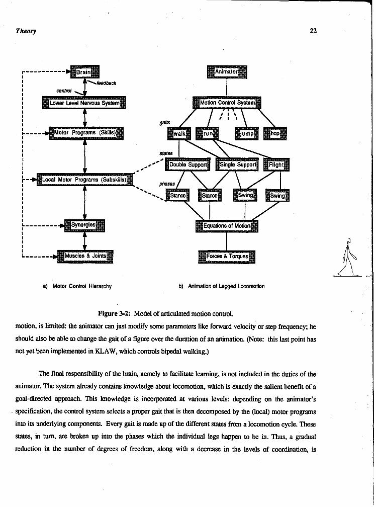
a) Motor Control Hierarchy b) Animation of Legged Locomotion
Figure 3-2: Model of articulated motion control.
motion, is limited: the animator can just modify some parameters like forward velocity or step frequency; he
should also be able to change the gait of a figure over the duration of an animation. (Note: this last point has
not yet been implemented in KLAW, which controls bipedal walking.)
The final responsibility of the brain, namely to facilitate learning, is not included in the duties of the
animator. The system already contains knowledge about locomotion, which is exactly the salient benefit of a
- goal-directed approach. This knowledge is incorporated at various levels: depending on the animator's
- specification, the control system selects a proper gait that is then decomposed by the (local) motor programs
into its underlying components. Every gait is made up of the different states from a locomotion cycle. These
states, in turn, are broken up into the phases which the individual legs happen to be in. Thus, a gradual
reduction in the number of degrees of freedom, along with a decrease in the levels of coordination, is

Theory
achieved by the control system which parallels that of its natural, biological counterpart. In KLAW, the
phases get further subdivided (STANCE1 to STANCE4 and SWING1 to SWING3) to restrict the range of
possible movements for the dynamics and to adapt the motor system to special cases in locomotion (see
chapter 6). At the bottom level, knowledge is represented by the dynamic equations of motion. Like the
synergies, these equations are tailored to perform a specific application, and therefore, in a sense, are kept at
a minimal number which proves to be advantageous when solving them (see section 4.5).
It is worthwhile to notice that the hierarchical illustration of figure 3-2 explains the decomposition of
a task or skiU quite well, but does not reveal all aspects of the control mechanism for locomotion. All gaits,
once a constant forward progression has developed, are characterized by cyclic or rhythmic activities of the
legs. Studies in Neurophysiology have led to the hypothesis of spinal pattern generators in vertebrates that
are responsible for stimulating the proper muscles to drive the legs through their cycles [Pearson 76, Path
851. There also seems to be some means of peripheral feedback, whereby sensory signals can influence the
output of the pattern generator such that, for example, an obstacle on the ground could trigger the swinging
leg to be lifted higher than usual in order to clear the obstacle.
For computer animation, it has been suggested [Zeltzer 82bl that the pattern generators, which are
represented by the local motor programs for the various phases of the legs, like left stance or right swing,
could be modeled by finite state machines. A similar approach was taken here. In KLAW, the successive
execution of the states for double support and single support maintains the cyclic locomotion pattern. A
transition between states occurs when the time for the current state has been exceeded. Within a state, the
different phases are executed concurrently: during double support, both legs are in their stance phases; in
single support, one leg is on the ground while the other one swings forward. The bookkeeping of what leg is
in which phase is done at the state level, and therefore, in a sense, by the finite state machine: one just
imagines that there really are two states for double support, one where the right leg is fmt (leading), and one
in which the right leg is the trailing leg. The single support state is split up as well, with the left leg in the
swing phase and the right one in its stance, and vice versa (see also figure 5-1). This method appears to be
flexible, and it is believed that it can be easily extended to control figures with more than two legs. Each
additional leg could be accounted for at the phase level and the program for the correct sequencing would be
. provided by the finite state machine. The dynamic equations would stay the same, since all legs go through
the same phases, just shifted in time. Also, by the same token, different gaits are merely a timing problem, as
indicated in figure 3-2 (b) for walking and running. In both gaits, the left and right legs occupy stance and
swing phases represented by the same sets of equations of motion. It is the relative timing, and the degree to
which the phases of the two legs overlap, that determines a gait. As the time for double support (stance

Theory
phases overlap) decreases in walking and eventually vanishes due to an increase in step frequency, the gait
changes to running. If the stance phases of the two legs move further apart, the time when both legs are in the
air becomes larger (the swing phases overlap). Thus, although in walking there is a double support state,
whereas running has a flight state, the individual legs still follow the stance-swing-stance cycle (see also
section 5.1).
The principle of sensory feedback, as introduced above, has been applied to the control structure in
two places: at the state level and the phase level. A locomotion step is defmed as one double support plus one
single support state. Before each step, the deviations between the current and the desired status of the system
determine the new configuration for the impending step. This might require a change in step length, step
frequency, or the rate of acceleration or deceleration of the figure. Of course, this type of feedback becomes
effective only when a change from the rhythmic pattern is expected, in particular at the beginning, during
start from rest, and the end of a locomotion sequence, when coming to a halt. Feedback at the phase level is
provided during the swing phase. If the figure was about to stub its toe or heel while trying to meet a desired
specification, the leg is raised just enough to clear the ground. This is explained in more detail in chapter 6.
3.3. The Refined Approach
In the previous section, a rough outline of the hierarchically organized algorithm to animate the
locomotion of legged figures was presented. The underlying idea is unique in that an attempt has been made
to tie together a high-level, goal-directed control and dynamic analysis. The approach is different in principle
from a pure dynamic method [Armstrong 85, Wilhelms 851, where the user is forced to specify movements
nonintuitively in terms of forces and torques. It also goes beyond a straight goal-directed system like
SA [Zeltzer 82b], in which, indeed, a task like walking gets decomposed step by step, but at the lowest level,
the output, that is the actual joint angles over time, are obtained from clinical data and interpolation
techniques. This is a bottleneck that makes it impossible to easily produce variations of a walk. The
interpolations, in a sense, have here been replaced by the dynamic equations. The dynamics create some sort
of an implicit control by autonomously performing elementary movements. The rationale behind the
approach as indicated in figure 3-2 is really twofold. There has been an effort to imitate, to some extent, how
. living vertebrates control locomotion (hierarchical structure), and to simulate how the motion actually gets
executed (dynamics).
Figure 3-3 gives a more detailed picture of the control algorithm. It should be regarded as a further
iteration of figure 3-2, now showing the information that has to be given or that has to be calculated at each

Theory
level. At the top, the animator specifies certain parameters. Besides simulation time, body height, and body
mass, there are three fundamental locomotion parameters that largely determine the patterns of motion and
gait the desired forward velocity (vk), step length (slks), and step frequency (gds). Their relationship is
expressed by the following simple equation:
V& = slk ' g* (3.1)
A major concern in constructing a goal -k ted system has been the degree to which a task should
be parameterized. The animator should have access to a simple, yet flexible set of movement commands that
can generate a variety of instances of a task. In KLAW, therefore, in addition to the locomotion parameters,
the user may specify up to 28 locomotion atm'butes which individualize the basic locomotion pattern. Among
these attributes are a stride width factor (lateral distance between the feet), the amount of toe clearance during
swing and the maximum rotation of the pelvis. A complete list and explanation is given in appendix E.
After the specification of the parameters, the system does all the necessary computations and outputs
the body angles as a function of time; these can then be taken to drive an animation of a legged figure. The
essence of the algorithm lies in its two levels of abstractions. Bearing the hierarchical structure in mind, these
two abstraction processes could also be viewed as a topdown, stepwise application of high-level concepts
and a bottom-up, physical construction of the necessary elements for legged locomotion; they are joined in
the middle by the gait-state-phase reduction mechanism already discussed above.
The conceptual level contains a few gait-specific rules or laws. They are utilized to transform the
locomotion parameters into some gait-phase constraints which are fed to the low-level control to "guide" the
dynamic simulation. In more concrete terms, the high-level control box performs the following tasks: first,
since at least one of vh, $IdcS and sfk have to be specified by the animator, the system completes (if not
all three parameters are input) and checks the locomotion parameters by the principle of the normalization
formula and equation (3.1). At the same time, depending on slks and .rfds, the gait (walking or running) is
determined. Subsequently, the application of the symmetry of steps concept and the evaluation of state-phase
timing functions yield the times and final angles for the stance and swing phases (see chapter 5). This
infoytion is passed to the low-level control, where it forms the consaaints for a special kind of boundary
value problem [Burden 851, which is evaluated with an approach somewhat like a shooting method. That is,
the equations of motion for the lower body are solved by interpolating the forces and torques until the
constraints are satisfied. For example, the simulation of the swing leg is repeated by varying the joint-torques
until it swings forward in the exact time required and heel-strike occurs with the desired hip and knee angles
(see chapter 4).

Theory
I I I
I I Conceptual Abstraction I
I !
I States
I
Gait h s e Constraints
I low-level Control
I I
I I
I I I I I
I
Physical Abstraction \ \ 1 \ \
LOG Body
Figure 3-3: Schematic diagram of the control system for legged locomotion.
Although the implementation is quite complex, using eEcient interpolation techniques, a solution is
usually found in a few iterations. A principal objective is to keep the dynamics simple, otherwise this internal
calculation of the forces and torques becomes infeasible. Since in legged locomotion, the activities in the legs
play the dominant role and most of the motion is directed forward in the sagittal plane, a basic two-
. dimensional, dynamic model of the lower body (the upper body is represented by just a single segment) has
been proven to be quite sufficient. Consequently, as long as there is at least one foot on the ground, the
number of degrees of freedom amounts to five, and during the flight phase in running, the model is
characterized by seven degrees of fieedom (see appendix C. 1).

Theory 27
The dynamic simulation produces the generic locomotion pattern which is visually upgraded by
kinematic measures. The rotation of the foot is added to the dynamic legs, a thigh and shank are
superimposed onto the telescope stance leg, and gait determinants like pelvic rotation or list get injected into
the one-hip dynamic model. It is important to notice that, even though a considerable amount of kinematic
"cosmeticsn are applied, the dynamics are the very heart of the control for they guarantee the natural looking
rotational movements of the legs plus smooth transitions between the phases and states. In a way, the
equations of motion guide the lower body kinematics, but because both are executed simultaneously, the
kinematic computations might, in turn, affect the dynamics. For instance, the simulation of the swing leg,
where the foot is assumed to be locked, has to take into account the updated position of the heel resulting
from the kinematic foot rotation in order to detect heel-strike properly at each time step. Similarly, the
kinematic pelvic rotation can actually lower the hip during the swing phase, which might "force" the dynamic
leg to increase its hip torque to avoid stubbing its toe.
Once the angles are calculated for the joints of the lower body, the motion of the upper body is
determined. This is done with the assumption that the upper body follows or depends on the lower body
movements. The arms, for example, swing forward with the opposite legs. Thus, the angles of the arms, as
well as the rotations in the shoulder and spine which compensate for the motion of the pelvis, are expressed
as simple (at the moment linear) hctions of the corresponding angles in the lower body. With this approach,
a total of 56 angles for 37 joints of the body plus a position vector in space are computed for each time step
(24 of these joints model the vertebrae in the spine; a complete list is given in appendix B.2).
One crucial aspect of the algorithm illustrated in figure 3-3 has not been mentioned in the above
discussion: the whole top-bottom control StnmKe is applied relative to a locomotion step. The constraints on
the motion calculated by the high-level control are updated before each step. In this way, the system achieves
autonomy in that it is able to adapt to changes in the locomotion parameters on a step to step basis. In other
words, the granularity of the system is one step. (At the end of the previous section, this mechanism was
indicated when discussing feedback at the state level).
In the.following chapters, the elements in figure 3-3 are addressed in more detail. The next chapter
introduces techniques related to dynamic analysis, in particular how the equations of motion are derived and
solved. The concepts of legged locomotion like symmetry of steps, and the mechanics such as the
determinants of gait are explained in chapter 5. Chapter 6, then, brings all these aspects together again while
discussing implementational issues.

Low Level Control Principles
Chapter 4
Low Level Control Principles
4.1. Multilink Structure
For the analysis and composition of human movements, the body sections that generate a motion are
usually modeled as a series of interconnected, rigid segments of constant length. Rotational joints represent
the points of articulation between the segments.
homogeneous transformation matrix in 2-D as
I cos Oi sin Oi
Ai = -sin Bi cos Oi O O 1 The orientation of each segment i is described by a
The joint variables Oi can be expressed in two ways: as absolute limb segment angles or as relative lI joint angles (figure 4-1). The former define the orientation of a segment independent from the other
segments. This approach is used for the simulation of the stance phase (see appendix C.l) in order to specify
the upper body angle with respect to the hip (which is the center of the whole body) rather than relative to the
origin of the dynamic model, which is set to be the stance foot.
More commonly, however, the orientation of a segment within a multilink structure is specified
relative to its parent in terms of joint angles. Each segment has its own local coordinate system
(transformation matrix) with the property that changing any joint angle does not require a change in all the
successive joint angles further down the chain. The absolute orientation of a segment i is calculated by
n;* A,.
To simulate articulated motion (as opposed to just animating it), the mass, center of mass, and the
distribution of mass around the center of mass for each segment also have to be known. The masses are
assumed to be constant and the segments to be symmetrical. The latter implies that the principal axes of

Low Level Control Principles 29
inertia are identical to the anatomical axes of rotation, and therefore the products of inertia are zero. Thus, the
distribution of mass is solely defmed by the moments of inertiaA which are calculated as described in
appendix B.1. It is submitted, that this simplification (i.e. to assume symmetry in segments) is justified for
dynamic analysis in computer animation, since it has no significant effect on the motion.
a) joint angles b) limb segment angles
Figure 4-1: Examples of multilink structures.
Assume Oi to be joint angles. The position vector pi to the center of mass of segment i, as illustrated
in figure 4-1 (a) is defined by
pi = UCl -
and pi = li = P = Ucl =
i i-1 j (gAj) I o , , o ~ ~ , where 'i-1 = P - ' [nAk) [O,$,O]T)
the proximal distance to the center of mass of segment i length of segment i the position vector connecting the body to the inertial (world) coordinate system the position vector to the distal end of segment i-1 .
If the system is expressed by limb segment angles, pi is calculated as follows:
Pi = - A 0 , r , 1 and viql = P - [z The pi, including their derivatives, make up the translational motion of the centers of mass and are
used in the process of deriving the equations by the variational principle.

Low Level Control Principles 30
4.2. Lagrange's Equations
The dynamic behavior of a physical system (in this case, of an articulated body) is defined by its
equations of motion. In classical mechanics there are two fundamentally different approaches to derive these
equations: vectorial mechanics and analytical, sometimes also referred to as variational mechanics. The
former is a direct application of Newton's laws, which requires the individual components of a system to be
analyzed in terms of vector quantities like force and momentum. The forces of constraint, such as joint
forces, have to be explicitly calculated. I
The analytical approach, on the other hand, provides a more general study of motion which is of
higher mathematical abstraction. A system is considered as a whole by means of two scalar quantities: the
kinetic energy and the work function. Constraints due to the structure of the system are determined
implicitly, i.e. they are automatically included in the equations. The entire set of equations of motion is
developed h m a unified principle, where the calculus of variations is employed to fmd the stationary value
of a certain action integral. Equation (4.3) below basically represents the solution or necessary condition for
this integral to have a stationary value. Details about the theory of analytical mechanics are provided in
[Wells 671 or Weirwitch 701. This mathematical approach is entirely independent of any particular
reference system, and therefore it is possible to adapt the coordinates to the specific structure of a model.
The analytical principle has been formulated in various ways, most importantly by D'Alembert,
Hamilton and Lagrange. Although they are all equivalent, in that they were derived from Newton's laws and
the concept of virtual work [Wells 671, it was decided to use Lagrange's formulation because it seems to be
most sophisticated, convenient and simplest to apply as a system gets more complex.
The Lagrange equations for a system with n degrees of freedom can be written as
, where r = 1 , 2 ,..., n and
L = Lagrangian = T-V T = Kinetic Energy V = Potential Energy q, = Generalized Coordinate F = GeneralizedForce . 4,
By determining the kinetic and potential energies for a particular mechanical system and
differentiating the Lagrangian according to equation (4.3), an ordinary, second order, nonlinear set of
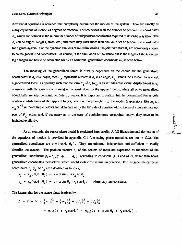
Low Level Control Principles
differential equations is obtained that completely determines the motion of the system. There are exactly as
many equations of motion as degrees of freedom. This coincides with the number of generalized coordinates
q,. , which are defined as the minimum number of independent coordinates required to describe a system. The
q, can be angles, lengths, areas, etc., and there may exist more than one valid set of generalized coordinates
for a given system. For the dynamic analysis of multilink chains, the joint variables ei are commonly chosen
to be the generalized coordinates. Of course, in the simulation of the stance phase the length of the telescope
leg changes and has to be accounted for by an additional generalized coordinate a , as seen below.
The meaning of the generalized forces is directly dependent on the choice for the generalized
coordinates. If q, is a length, then F represents a force; if q, is an angle, F stands for a torque. In general, qr qr
a generalized force is a quantity such that the term F - 64, (64, is an infinitesimal virtual displacement in q, qr
consistent with the system constraints) is the work done by the applied forces, while all other generalized
coordinates are kept constant, i.e. only q, varies. It is important to realize that the generalized forces only
contain contributions of the applied forces, whereas forces implicit to the model (expressions like m2 h, m2 a 8: in the example below) are taken care of by the left side of equation (4.3); forces of constraint are not
part of F either and, if necessary as in the case of nonholonomic constraints below, they have to be qr
included explicitly.
As an example, the stance phase model is explained here briefly. A full illustration and derivation of
the equations of motion is provided in appendix C.l (the swing phase model is set out in C.2). The
generalized coordinates are q,. = ( 0 , el, O2 ) . They are minimal, independent and sufficient to totally
describe the system. The position vectors pi of the centers of mass are expressed as functions of the
generalized coordinates pi = pi ( ql, q2, . . . , q, ) according to equations (4.1) and (4.2), rather than being
generalized coordinates themselves, which would violate the minimum criterion. For instance, the cartesian
coordinates x2, y2 of pZ are calculated as follows,
5 = 3 ( 0 , 0 ~ , 0 ~ ) = ~ + o s i n 0 ~ + r ~ s i n 0 ~
y2 = ~ ~ ( 0 , 0 ~ , 0 ~ ) = y + ~ c o s 0 ~ + r ~ c o s 0 ~ , wherex,yareconstants.
The Lagrangian for the stance phase is given by

Low Level Control Principles 32
With this, differentiation of equation (4.3) yields a system of three equations of motion, where the
generalized force F, is a force along the leg axis, F and F represent torques about the foot and the hip 9 92 for the upper body, respectively:
It should be noted that the Lagrangian approach, as stated above, is only applicable to holonomic
systems. This requires that the coordinates qr are independent, which is assumed by the definition of
generalized coordinates. If constraints are present, they must be expressible in a simple algebraic form
Xi =xi (ql, q2,. . ., q,) , so that superfluous coordinates can be eliminated directly (see also degrees of
constrain@). Holonomic constraints reduce the degrees of freedom and consequently the number and
complexity of the equations of motion as well. For completeness, although there is no relevance to this
application, it is mentioned that the problem of nonholonomic constraints (as long as they are of the type
r=l ar.6qr = 0, where ar are fmctions of the coordinates qr), which can not be integrated, may be solved
by the method of Lagrange multipliers IJvleirovitch 701. The forces of constraint are now explicitly specified
in equation (4.3) by adding the term hc.acr to the right side for each constraint c .
It should be understood that the Lagrange equations or any of the other approaches, including the
direct application of Newton's laws, are merely a means to construct an eventually equivalent set of
equations of motion for a given system. The problem of solving the equations is addressed in the following
section.

Low Level Control Princ@les
4.3. Integrating the Equations of Motion
The equations of motion can be solved in two ways. The method of Inverse dynamics calculates the
forces given that the motion of a system is specified If qr, 4 and are known over the duration of the
motion, this amounts to the algebraic evaluation of a discrete set of equations for each time step, where the
solution at time t has no effect on the equations at time t + At.
Forward dynamic analysis is the determination of the motion of a system given the forces; they
involve integrating a coupled system of second order, nonlinear differential equations. The solution process
is continuous, in that the output from one time is the input to the equations at the next time step. In this thesis,
forward dynamics were applied to calculate the joint angles over time. Interpolation techniques were
employed, as discussed in a subsequent section, to approximate the force and torque profiles, that produce a
desired locomotion cycle, but are unknown a priori. This approach should not be confused with inverse
dynamics. It resembles more a boundary value problem since only the initial and final values for certain
variables, as well as some timing constraints, are provided rather than predefming the complete motion (see
section 4.5).
Because there are no analytical solutions, the equations of motion are integrated numerically. For
this purpose, the equations are written in matrix form
~ i i = ~ ( q , q ) ,
where A = inertia matrix (n x n matrix for n degrees of freedom) q = solutionvector B = vector of transient terms (including the generalized forces) .
For example, the three equations of the stance phase as formulated in the previous section have the
following matrix form:

Low Level Control Principles
Note that due to the structure of the system, A is symmetric. Initially, the following simple
combination of an explicit and implicit Euler method was used to integrate the equations:
q ( t + A t ) = q ( t ) + A t q ( t )
q ( t + ~ t ) = q ( t ) + ~ t q ( t + ~ t ) .
I
After careful analysis of the resulting motion, it became obvious that the method was only I
reasonably stable if the initial conditions ( q, q, q ) were kept close to zero and no external forces were
applied, i.e. the system was conservative. This was not acceptable since a major aspect of the locomotion
algorithm requires the presence of controlling forces to achieve a variety of movements. The instability of
Euler's method was somewhat expected because of the several springs and dampers in the system which
cause the problem to be stiff Purden 83. No formal analysis of the eigenvalues was done to check whether
they lie within the stability region of the numerical method, which is to verifj. that the errors were introduced
by the integration process and not due to an inaccurate dynamic model. Since the system is nonlinear, the
eigenvalues are not constant and would have to be numerically calculated.
For simulating the motion of a multilink system, an A-stable method [Burden 851 such as
LIMEX [Zugck 841 or LSODI lHindmarsh 801 is preferred, that has a large stability region covering the
entire left half of the complex plane. The LSODI integration package was eventually chosen, which produced
reliable results for this thesis. LSODI solves the initial value problem for an ordinary system of first order
differential equations. It was therefore necessary to transform the second order equations A q = B ( q, )
into a first order representation A' u = B'( u ) , where the solution vector u is of the form [Burden 8 3 -
'2i-1 - 4i - u~~ - u S l = q for i = 1 , 2 ,..., n .
This transformation essentially doubles the number of equations (see appendix C for stance and
swing phase). Frequently, standard integration techniques require the specification of the Jacobian matrix J a bti
(with jik = - ; i, k = 1,2, . . . ,2n ) of the transient terns. LSODI has to be supplied with the full Jacobian 8%
matrix defined by

Low Level Control Principles
and the vectors is an internally generated approximation to u .
4.4. External Constraints
The motion of an articulated body (in general, any physical body) is a result of its interaction with
the environment and therefore subject to external constraints. For legged locomotion, the principal constraint
is imposed by the ground. It enables the body to transform its rotational movements around the joints of the
lower extremities into an overall manslation in space. There have been different approaches in human motion
simulation as to how the constraints should be mathematically formulated and included into the model.
Wilhelms [Wilhelms 851 makes use of springs and dampers to confine the motion of body segments.
Consequently, an stiff system is induced that might lead to integration e m . This is especially
the case for simulating ground contact, where large spring and damping constants are required to keep the
foot, which wries the whole body weight, on the ground Although this method is not employed here to ? express external constraints, springs and dampers are introduced at two places to maintain internally desired h states: they control the torque values F to balance the upper body, and F at the end of the swing phase to
'32 O3
keep the desired hip angle fixed until heel strike( see chapter 6).
A more appealing approach to the application of external constraints is to analytically constrain the
motion of the model by reducing it to a subspace of smaller dimension. The ground constraint during the
stance phase was represented this way. Since the foot of the dynamic stance model does not move (the added
kinematic foot does as explained in section 5.4), only three degrees of freedom ( a , el, e2 ) are necessary to
describe the system. If, on the other hand, the constraint was relaxed, as during the flight phase in running,
the changing position of the foot would have to be accounted for by two additional degrees of freedom (in
total, x,y, a , el, O2 ).' In general, this approach involves the derivation of two sets of equations for the
system, one for which the constraint is active and one for which it is inactive. Unlike the spring and damper
method, constraints here do not complicate the actual integration process because the extra amount of work is
done beforehand when deriving the equations.
Legged locomotion can be characterized as a cyclic activity where each leg follows a strict
alternation of stance and swing phases ( see section 5.1). In terms of ground constraints, this means that they

Low Level Control Principles 36
have to be "turned" on or off with every phase change; using the above technique, this is identical to
switching between equations of motion. In order to produce smooth transitions, i.e. a continuity in
movements across phases, the equations of a new phase have to be initialized properly. In particular at heel
strike, which occurs between the swing and the stance phase, some extra measures have to be taken to
correctly capture the abrupt change in the motion of the leg. The problem can be expressed as a mechanical
collision between the leg and the ground. For this purpose, the simplifying assumption is ma& that the
support is transferred instantaneously at impact from the hind to the front leg, even though in bipedal walking
the body weight is really shifted between the legs over the duration of the double support phase (in running,
this assumption would not be necessary since the body is airborne before heel strike). It is also assumed that
the spring in the leg of the stance model (see figure C-1) is massless, so that for an instant after ground
contact, there is no reaction force (or velocity) along the leg axis and therefore the linear momentum P, is
conserved during the collision. Since the angular momenta of the foot L and the hip L of the stance leg At h*
are conserved as well, we can write
where - means before, + after impact. From these equations (for details see appendix C.3) the thaw -dl.- ,. .: velocities after impact c?, 8;. 8; can be calculated and input initial conditions (together with o, el, O2 )
into the subsequent stance phase.
The formulations of the linear and angular momenta above imply that the physical models before
and after heel strike are described by the same coordinates; but this is not the case, since the swing leg was
defined earlier as a double pendulum in terms of O3 and 04, and not by o and O1 (see appendix C).
However, as will be discussed in detail in chapter 6, the knee of the swing leg is extended and "locked"
shortly before heel strike. Therefore, the model of the swing leg is transformed into a single pendulum of
fmed length I and hip angle 034 (which can be substituted into the above linear and angular momenta
equations for o and el , respectively). The extension of the knee between the double and single pendulum
. subphases is a collision that, analogous to above, determines the value of $4 (only one equation is needed,
see appendix C.3) based on the conservation of angular momentum at the hip of the swing leg

Low Level Control Principles
The simulation of constrained motion and the application of the laws of collision, as approached in
this section, are good examples of areas in computer animation where dynamics are clearly better than pure
kinematic techniques.
4.5. Interpolation of the Generalized Forces
So far, the equations of motion have been presented as an initial value problem of the fcnm
A' u = B'( u ) for every phase, given the initial condition u ( to ) = a. However, this method can not be used
to produce a realistic locomotion cycle, not to mention a variety of locomotion sequences. Although it is
possible to apply different initial conditions as well as force and torque values, no mechanism is provided to
enforce a desired motion. The problem is therefore redefined for each stance and swing phase:
A'U = Bf(u,F ), subjectto u ( to )=a , u($)=P and t O < t l t e . 4,
(4.4)
Two new constraints are introduced specifying the values of the generalized coordinates at the end of
a phase (final conditions) and the duration of a phase. These constraints are determined for each instance of a
phase by the higher level control principles as explained in subsequent sections. The generalized forces F qr
are now expressed as independent variables of equation (4.4). If the general solution to the problem is written
as
u = f( t ,F , C ) , qr
which is a classical root-finding problem where the roots F are approximated by interpolation techniques. 4.
In practical &ms, the objective is to find the proper forces or torques such that, given the initial
conditions u( to ) , the system reaches the final conditions u( te ) in exactly time re . A s an example, the stance
phase is considered here: the initial conditions come from the preceding swing phase and the collision laws
'(as already discussed). The final conditions are the hip angle ds and the length of the leg a,, at time - tsee. The equations of motion are now integrated over the duration tslonce in a loop by modifying the hip
torque Fg and the leg axis force Fw until the final conditions are met. 1

Low Level Control Principles 38
The interpolation of F is performed in two stages. First, the Bisection method computes a qr
reasonable approximation which is then refined by the Secant method. This technique was employed because
the Secant method converges fast, but needs a good first approximation (see Burden 851). The upper and
lower bounds for F to start the Bisection method are determined by the following simple algorithm, which qr
ensures that there is a root between the bounds and that they are no more than i n c apart; it is shown for the
stance phase, where F represents the hip torque:
F = F ini t ; - upper = lower = false; while ( !upper l l !lower )
integrate equations from t = to t o t = tatma;
if ( 8, (tstma ) < 8,-dJtattuur 1 ) lower = true; F-lower = F; F = F + inc;
else upper = true; F-upper = F; F = F - inc;
endif endwhile
A solution to F using the above interpolation technique is usually obtained within a few iterations qr
(between 6 and 10). Once the rhythmic phase of a locomotion sequence is reached, i.e. the forward velocity
of the body as a whole is fairly constant, the algorithm converges even faster since the F profiles from one qr
step (stance + swing) are carried over to initialize the next (F - init above). It should be noted, though, that
some of the F are actually represented by functions of time and other parameters, that is, they are not qr
applied uniformly over the duration of a phase. This aspect is dealt with in chapter 6. (Aside: from a
neurophysiological viewpoint, the process of forwarding the leg torques F from one step to the next could qr
be considered to represent the muscle memory of the lower level nervous motor program for walking as
described in section 3.2. )

High Level Control Concepts
Chapter 5
High Level Control Concepts
In the last few sections, the study of legged locomotion focused on a simple dynamic model, whose
internal structure was specifically designed to naturally support bipedal walking. The equations of motion,
therefore, can be regarded as the functional synergies of the motion control hierarchy in figure 3-2, that are
capable of executing a definite range of locomotion patterns under the control of specialized motor programs.
Each motor program "knows" about a particular action. To this extent, the discussion of the locomotion cycle
in the subsequent sections and the conclusions drawn essentially symbolize the motor program for bipedal
locomotion.
Another analogy might be opportune: if one were to view walking as a programming language,
virtually compiled by the control algorithm devised in this thesis, the dynamics in the preceding sections
could represent the syntux of the motion, whereas the walking semantics would be inherent to the conceptual
understanding or knowledge of the locomotion cycle. In the following, then, a "meaning" is given to the
dynamics by bringing the two aspects together. In particular, it is shown how the conditions for each phase
can be derived to solve the problem as formulated in equation (4.4), i.e. how to guide the dynamic model.
Also, knowledge of the leg kinematics is utilized to visually upgrade the basic locomotion pattern which is
generated by the dynamics.
5.1. Locomotion Cycle Characteristics
Generally, a sequence of animal locomotion can be subdivided into three stages: a short developing
period characterized by an increase in speed, followed by a dominant rhythmic period where the forward
velocity is kept fairly constant, and a brief &cay period to decelerate the body. Almost all research on
locomotion concentrates on the rhythmic phase of a gait on level surface; very little is known about how the
basic pattern of each individual subject changes under the influence of acceleration, deceleration, or by going
up and down inclines. Since rhythmic locomotion is just a series of recurring movements with the natural
period of one stride (locomotion cycle) for every gait and any number of legs, it is sufficient to just direct
investigations, as well as present kinetic and kinematic results, relative to one cycle.

High Level Control Concepts 40
The human walking cycle has been thoroughly studied. A good reference is a book by Inman [Inman
811, which includes a lot of experimental data from various authors. For bipedal walking or running, a
locomotion cycle consists of two steps. As long as a symmetric gait (see gaitA) is assumed, where the left and
right leg perform the same movements, just out of phase, the principal unit of locomotion can be reduced to
one step. There are two independent parameters (expressed in terms of the step unit) to define a specific
instance of a gait step length (sl ) and step frequency (sf). Together with their product sl - sf which is the
speed of the locomotion (v), they form the three locomotion parameters as introduced in section 3.3.
Walking is possible at a wide variety of combinations of sl and sf. However, a person, when asked to walk at
a particular velocity, is most likely to naturally "choose" the parameters which minimize energy expenditure.
This observation is expressed in the experimentally derived equation Fman 811, called nomlizing fonnula,
which shows a linear relationship between sl and 4 , where sl and body-height are measured in m, sf in
steps1 min :
sl = 0.004 e sf2 = v V
sf- body-height , because of sl = - . (5.1)
0.004 - body-height sf
The body-height normalizes the equation. It indirectly represents the length of the legs, which, of course,
have an effect on the preferable step length. As stated in [Inman 811, equation (5.1) is based on data almost
exclusively obtained from male subjects; women tend to walk with a shorter step length and greater step
frequency at a given speed. Also, the normalizing formula applies only up to a certain step frequency sfwm of about 132stepslmin (which corresponds to sl-=0.528.body-height), if the speed is increased after
that, the step length is kept constant. Another obvious condition to maintain a walking cycle is that neither of
the locomotion parameters is allowed to exceed a maximum value (sl-=0.6-body-height,
sfIMX = 182 stepslmin , vmar = slnorm- @- ), otherwise running would result. Although the limits on the
locomotion parameters as specified are quite constant for different subjects, they can be changed by the user
for experimental purposes as part of the locomotion attributesE.
Given equation (5.1) and the above constraints, an algorithm (for details see appendix D) is now
designed to supplement the remaining locomotion parameters, if at least one is specified. For instance, if a
velocity is defined, a "natural" step length and step frequency are calculated; in the case where a step length
and step frequency are specified (assuming these as well asithe resulting velocity are within the anatomical
limits), a more angular motion might result.
Once the locomotion parameters are complete, the step frequency is used, as shown below, to derive
the state-phase-timings, whereas the step length is applied to the symmetry of steps concept (section 5.2) in

High Level Control Concepts 41
order to compute the final conditions for each phase of the current step. Hence, the two, up to now still
undetermined ingredients to the central problem stated in equation (4.4) are deduced.
HSR T a HSL
I d% 1 step 5 0 %
a) walking cycle HSL = heel strike left TCR = toe off right HSR = heel strike right TOL = toe off left
HSL TOL HSR m HSL
I I . d% 1 step 5 0 % 1 0 0 %
b) running cycle
states
phases
Figure 5-1: Locomotion cycles for bipedal walking and running.
single support (left)
I
left stance < **
right swing ------
single support (right)
left swing
right stance b*
flight D-I
flight b-
* D*

High Level Control Concepts 42
As already mentioned, a walking cycle consists of two steps. From figure 5-1 (a), it can be seen that
each step contains one double support state (ds ) where both feet are on the ground, and one single support
state (ss ) where one foot is off the ground. Formally, assuming t to denote a duration, this can be written as
In terms of the individual legs, which go through the same stance-swing-stance cycle, just shifted in time, the
following holds:
- %eP - tstance - tds (5.2)
- tstep - + tds '
Experimental data gathered by different authors (see [Inman 811) suggest a linear relationship in
walking between the step frequency (sf) and the double support state as a percentage of a cycle. After
interpolating the results from the different experiments, the time for the double support (t, ) amounts to
t, = (-0.16-sf + 29.08) tcyCIe 1100 . (5.3)
Since sf is known as one of the locomotion parameters, and because of
- 2 'cycle = 2. 'step - - sf '
tds can be determined, and consequently the values for tsa, and twhg are obtained from equation (5.2).
The above calculations form the basis of the state-phasetiming concept. Although not directly
relevant, a few remarks on walking vs. running (see figure 5-1) pertain to reveal similarities between the two
gaits: equation (5.3) expresses the fact that with increasing step frequency, or speed in general, the time for
double support decreases in walking. At the phase level, this means that with bigger sf the amount of overlap
between the stance phases of the legs is diminishing. When sf reaches about 182stepslmin (sf-mux), the
double support state disappears. At this point, walking is equal to running. If the step frequency increases
further, tds in equation (5.3) becomes negative, which signifies the flight state, where both legs are off the
ground; in other words, the swing phases start to overlap. Abstractly speaking, the two diagrams of figure
5-1 are quite similar. In going from walking to running, the right vertical bar indicating the end of double
support is just "slid" to the left, and as soon as TOL comes before HSR (i.e. the left leg enters the swing
phase before the right leg terminates its swing phase), the gait changes to running. Thus, if there exists a
relationship between the step frequency and $,igh, running could be implemented by the same technique. Of
course, running is not just possible when the sf exceeds sf-mux, but generally, can also take place for the

High Level Control Concepts 43
same locomotion parameters as walking. In figure 5-1, both diagrams are based on the same time for a step,
that is the same step frequency, and reasonably so, equal step length. To cover all of these possibilities for
"artificial" running, additional information would be required such as the relationship between the maximum
vertical distance between the foot and the ground during flight and $ig,,, .
5.2. Symmetry of Steps
If one were to have stiff legs (no knee joints) and no feet, the only way to move forward would be by
means of a compass gait as shown in figure 5-2. For planar motion, the leg would drop below the ground
during its swing phase. An interesting fact about this simplest form of bipedal locomotion is step symmetry.
At heel strike, provided that both legs are of the same length, the angles of the legs measured from the
vertical are identical, that is el = 8.3 at times tl , t2 and t., , and only depend on the step length sl. Most
importantly, this still holds m e when the body is accelerating or decelerating, which is indicated in figure
5-2 by the increased step length at time t3 (i.e. the body accelerated from t2 to t3 ).
LL = left leg RL = right leg
Figure 5-2: Symmetry of compass gait for different step lengths.
It should be noted that the concept of step symmetry introduced here is different from elsewhere in
the literature Daibert 86a], where symmetry is defined for the stance phase relative to the center of mass
(which is located at the hip in the model). In this case, symmetry is only maintained if the step length does
High Level Control Concepts
not change, which means there is constant speed. Thus, as shown in figure 5-2, the angle e3 of the left leg at
the beginning of the stance phase at time t2 is not equal to the angle el at the end of the stance phase at time
t3; whereas $ at time tl would be the same as at time t2 for the stance phase of the right leg.
The symmetry of step principle is now adapted to the model in figure 5-3 to determine o , and e3 at the end of a step (heel strike). Although the actual step configuration at heel strike is is not symmetric any
more because of the introduction of a kinematic foot for the swing leg, the basic idea can still be applied. We
just imagine the symmetric step situation when the foot is flat on the ground some time after impact
(illustrated by the dashed line) and calculate "back in time". For this purpose, the step length sl is measured
between anklel and ankle2. The effect of the foot at heel strike is really that the absolute value of O3 is
smaller than it would be in the absence of a foot (it also holds that O3 < el ). In addition, the foot raises the
position of the hip at impact, which has to be compensated by lengthening the telescope stance leg beyond its
initial length, i.e. o > ll . Details about controlling the changing length of the stance leg are given in chapter
4. The origin for the simulation of the stance leg stays fured at anklel, which is at a distance lg above the
ground. It is important to realize that the kinematic foot of the stance leg can be ignored at this point. Since it
is superimposed on the motion of the dynamic leg after the simulation of the stance phase, it does not affect
the calculations here, unlike the foot of the swing leg. The stance foot is explained as part of the separate
concept of virtual leg in a subsequent section.
/ c.:: For the following calculations, it is assumed that the ground is at zero height and O5 at impact is
specified as one of the locomotion attributesE. In the actual implementation, a value for e4 (knee angle of
the swing leg) at heel strike may also be selected to prevent the knee from fully extending. This aspect is - 2 2 disregarded below for simplification (i.e. O4 = 0 and l 3 = 1 ) Given 1 , 1 and lg , ll = dl8 + lg and
'8 cos (a8) = are determined. The application of the cosine law yields
11
Since
addel = (xu, y,) = (x*, + IS, lg ) , where xnh, is xnh from previous step, and
it follows that

High Level Control Concepts
FiHre 5-3: Dynamic model at heel strike: the swing leg is extended, a foot has been added kinematically; is assumed to be negative, all other angles are positive.
One great advantage of step symmetry, as well as of the state-phase-timing concept from the
previous section, is that all computations are done relative to one step which is the impending step in a /
locomotion sequence. Changes in. the locomotion parameters sf and sf can therefore be accounted for with
the "granularity" of one step. This allows for acceleration and deceleration of the motion, and even the
extreme cases of starting from rest and coming to a full stop are possible (with minor adaptations of the
underlying dynamics as shown in chapter 6). On the last step, for instance, sf is set zero (no "ground is

High Level Control Concepts
gained" since the hind leg only pulls even with the front leg), which, in the above calculations, results in the
desired final conditions el = e3 = 0 and o = ll .
However, one danger exists in treating each step separately: extreme changes in the locomotion
parameters could cause large variations in the times and final conditions for successive steps, which, in turn,
would produce torque and force profiles in the dynamic model that exceed the natural, anatomical limits of a
human body. To avoid the problem, three locomotion attributes have been defined, vacc , vdcc and sfaccdec, to
restrict the amount of (constant) acceleration, deceleration or change in step frequency from one step to the
next (the latter became necessary, since even for fairly constant velocity, an increase in sf can result in
skyrocketing torque values). Further experimentation with the system is required to determine boundary
values for these attributes that are "reasonable" for bipedal walking.
So far, all the necessary information to control the dynamic simulation of the leg phases has been
derived. The next step is to concentrate on the details of the motion by adding kinematic, human-like features
to it. Although the dynamics of the walking model are self-sufficient, including lower body kinematics can,
in certain cases, have a direct effect on the dynamics. This was m e above, where the addition of a foot to the
dynamic swing leg changed the calculations of the final conditions for a step. Kinematics can also affect the
dynamics during the actual simulation. A good example is the animation of the pelvis, which basically
"splits" the dynamic hip into two, with the o r i g d hip remaining "on" the stance leg, while the motion of the
hip for the swing leg is expressed as a function of the former. Due to pelvic list (to be discussed in the
following section), the knee during the dynamic simulation of the swing phase now has to be flexed more to
avoid ground contact. Therefore, the dynamics and lower body kinematics must be executed concurrently.
A last note is directed to running. Extending the step symmetry concept to this gait would involve
the distance traveled during flight being subtracted from the step length sl before calculating the final
conditions for a step.
5.3. Determinants of Gait
The net result of a locomotion seqyence may be considered as a translational displacement in space. - However, the motion, when analyzed in more detail, exhibits subtle deviations from the line of progression
due to the rotational movements of the pelvis and the legs. During a locomotion cycle, the body rises and
falls slightly, weaves from side to side, as well as speeding up and slowing down a bit, even if the overall
forward velocity is constant. The displacement of the center of mass of the body, which represents the motion

High Level Control Concepts
of the body as a whole, is illustrated in figure 5 4 for one stride. The vertical displacement (A) prescribes a
sinusoidal curve with a maximum at mid stance and a minimum at heel strike. This component of the motion
is generated directly by the simulation of the telescope stance leg (see chapter 7 and appendix F). The curve
(B) caused by the lateral motion of the center of mass is also sinusoidal at half the frequency of the vertical
displacement. The lateral movements arise because the upper body is shifted over the respective weight-
bearing stance leg.
Figure 5-4: Exaggerated movements of the center of mass during one stride; different line spacing indicates a change in velocity (lines closer
together mean deceleration, larger line spacing acceleration).
There is a direct correlation between the motion of the center of mass and energy expenditure in
walking. Figure 5-5 shows the kinetic (translational and rotational), potential and total energy for half a
stride. Employing the concept that the weight of the upper body is a passive element, which is carried on the
active lower limbs [Inman 811, the enerp levels of the HAT (head, arms and trunk) are displayed, rather than
the energy profrles for the whole body. The potential energy curve is essentially identical with the vertical
displacement of the center of mass (see figure 54). whereas the kinetic energy changes with the forward
velocity of the center of mass. A maximum in potential energy, which coincides with a minimum in kinetic
energy, occurs at about the middle of the single support period, while the potential energy reaches a
minimum at the middle of the double support period, i.e. just after heel strike. At the same time, the kinetic

High Level Control Concepts
energy has a maximum value. The shapes of the two energy curves resen
48
rite well those of a
conservative physical pendulum (see figure 5-6). However, unlike in the case of a swinging pendulum, the
energy exchange is not complete. Even if the difference in magnitude between the kinetic and potential
energies is neglected, the total energy shows substantial fluctuations. Walking therefore is a nonconsemative
activity, where the losses in energy have to be "topped off" with the work produced by the muscles.
. walking cycle (%)
total energy
kinetic energy
potential energy
Figure 5-5: Approximations of kinetic, potential and total energy of the HAT for one walking step at average walking speed (adapted from [Inman 8 11). The total
energy is computed with the minimum potential energy level assumed at zero. The ordinate values in parentheses are for the potential energy.
time
Figure 5-6: Exchange of kinetic and potential energy of a pendulum (neglecting friction). The total energy is constant, thus the system is conservative.

High Level Control Concepts
From the above, it is concluded that smaller deviations of the center of mass from the line of
progression generate smaller fluctuations in the energy levels and consequently, the less energy is expended.
During human walking, the absolute location of the center of mass stays within the region of the pelvis
Fman 811. This is mainly achieved through the combined efforts of the &terminunts of gait.
Inman IJmnan 811 distinguishes between six determinants:
+ pelvic rotation (transverse plane)
+ pelvic list (coronal plane)
+ pelvic tilt (sagittal plane)
+ lateral displacement of body
+ knee flexion of stance leg
+ plantar flexion of stance leg ankle
Compared with the compass gait (already introduced in figure 5-2 as the simplest form of bipedal
locomotion), where the pathway of the center of mass is through a series of arcs, one for each step, each of
the above determinants smooths this path in one way or another to produce the sinusoidal curve of figure 54.
Whereas the movements of the pelvis just flatten the arcs, the combination of knee and ankle motion
alleviates the sudden changes in vertical displacement at heel seike, i.e. they remove the "tips" of the arcs by
transforming them into a smooth curve. From this point of view, the determinants of gait contribute directly'
to minimize energy expenditure. For the purpose of animating human walking, the determinants greatly
improve the realistic looks of the motion.
In the following, the determinants of gait are described in more detail. All determinants have been
incorporated into the walking algorithm except pelvic tilt, which was neglected because it did not appear to
have a perceptible visual effect in walking. Furthermore, the forward and backward tipping of the pelvis
mainly affects the upper body, which is balanced independently anyway (see section 5.5). For the
implementation, a kinematic pelvis and foot had to be added to the dynamic stance model. It is submitted that
all the determinants can be expressed as linear functions, although experimental results [Inman 811 suggest a
better approximation by higher order polynomials. This step is justified since the displacements generated by
each determinant are relatively'small (a few centimeters for the maximum values), so that the simplicity of a
linear approximation outweighs the little qualitative improvement of a more complicated function. Various
effects of the determinants on the motion are illustrated in appendix F.

High Level Control Concepts
Pelvic rotation about the vertical axis is a minimum at mid-stance and a maximum at heel strike. The
rotation causes a larger step length and consequently, a greater radius for the vertical arcs of the center of
mass. Since the step length, as defmed by the locomotion parameter sl , includes the maximal displacement
(from pelvic rotation) at heel strike, the actual step length used in the calculations of the step symmetry,
denoted sl-act for now, needs to be adjusted for each step:
sl sl-act = sl - sin (pelvicrOt ) . lo , where pelvic, = p e l ~ i c ~ ~ - ~ .- sl-rmUL
and lo denotes the width of the pelvis (see appendix B.l); p e l v i ~ ~ , - ~ is specified as one of the
locomotion attributesE. For each step, the rotation of the pelvis is now linearly incremented until pelvicrot is
reached at heel strike. This causes the hip of the hind leg (h, ) which is at a maximum behind the hip of the
front leg ($ ) at heel strike, to move forward faster than $ (by the increments) during the double support
and swing periods to eventually reach a maximum position in front of at the end of a step (see figure F-5).
Pelvic list is the rotation about the x-axis in figure 5-4 which makes the hip of the swing leg drop
lower than the hip of the stance leg. As an effect, the center of mass does not need to be elevated so much
and therefore the change in potential energy is reduced A maximum angle occurs, i.e. the swing hip is
lowest, just after toe-off, and thereafter the hip of the swing leg rises until it arrives at the same level as the
hip of the stance leg at heel strike. This last characteristic of pelvic list, that is to equal the height of the hips
at impact, is essential for the validity of step symmetry (which is based on a one hip model as shown in
figure 5-3). A natural pelvic list is implemented as follows: after the simulation of the stance phase, the
minimum height of the hip is computed, which comes shortly after heel strike (i.e. at the very beginning of
the stance phase), and taken as the value for the swing hip at the end of the double support period (toe-off).
The difference between this minimum hip value and the vertical position of the stance hip at toe-off yields
the maximum angle for pelvic list for that step. As above, linear interpolation is employed to fill in all the
remaining angles. A pelvic list factorE may be selected by the user to exaggerate or reduce pelvic list (see
figure F-7).
The lateral displacement along the z-axis in figure 5-4 represents a shift of the weight of the body
from stance leg to stance leg during a locomotion period (see also figure F-6). Moving the center of mass
closer to the weight-bearing leg results in less effort being required to balance the upper body. The lateral
displacement from the line of progression is a maximum at mid-stance and zero at the time of heel-strike
(again, a necessary condition for step symmetry). There are two variables which influence the magnitude of
lateral displacement, a stride width (sw ) measuring the lateral distance between the feet (in m ), and the step

High Level Control Concepts 51
frequency (sf). A bigger stride width causes the body to rock more from side to side, and with increasing
step frequency (usually synonymous with a greater speed), the lateral displacement decreases. The following
relationship has been established for the maximum lateral displacement (It-ma) for a step •’?om various
experimental results [Inman 811:
It-ma = -0.00017241-sf + i . s w + 0.0013448 .
A stride width factor is specified as a percentage of the pelvic width (lo) in the list of locomotion
attributesE, from which sw is then determined.
The knee flexion of the stance leg together with the plantar an&le flexion of the stance foot, fulfill
several functions. They serve as a major shock absorber at impact and smooth the transition of the stance leg
from the double support period to the swing phase. In particular, the foot also retains the center of mass in a
more elevated position at heel strike compared with a basic compass gait as was shown in figure 5-3. The
implementation of these determinants is more ambitious and treated separately in the next section, since they
involve the concept of a virtual leg.
5.4. Virtual Leg
The simulation of the stance phase based on the dynamic model of figure C-1 (a) generates the
motion of an inverted, length-changing pendulum for one "step" under the given constraints for time and
fmal conditions (it should be noted that the upper body is ignored in this discussion). What is desired, though,
is the realistic motion of a human leg during the stance phase, which inherits the leg determinants described
in the previous section. For this reason, a human leg may be superimposed onto the dynamic pendulum at
each time increment as shown in figure 5-7. Unfortunately, the number of possible configurations is infinite,
i.e. a unique solution does not exist for the orientation of the segments from the hip (H) to the tip of the toe
(T). This is a typical inverse kinematics problem, where the proximal (H) and distal endpoints are given
and the task is to find the angles of the kinematic chain spanned between these endpoints. At least two of the
four angles (e3, . . . , e6 ) must be known to fully specify a particular configuration. In order to predetermine
some of the angles so that the remaining ones can be determined unequivocally, additional information is /
required. In the present case, the information is supplied according to some general rules about the stance
phase, which is therefore subdivided into a normal, heel-off and meta-off period. These periods are strictly
successive in time and all three occur for any stance phase.
The normal period is illustrated in figure 5-8 (a). It characterizes the early state during stance,

High Level Control Concepts
Figure 5-7: Superposition of a leg over the dynamic stance leg model. The size of the rnid-foot (Il2 ) and toe (Il3 ) are exaggerated; the location of the hip (H )
comes from the dynamic simulation, for which anklel is assumed to be fixed at (xu, y,) . The tip of the toe (T ) maintains ground contact during the whole
stance phase at position (xu + l5 + 16, 0) ; 112 and 113 are simply defined
as 41; + 1: and 41; + (19 - G ) ~ , respectively (see appendix B. 1).
where, after heel strike at time to the foot is rotated about the heel to come down onto the ground, and
subsequently stays flat on the ground (e.g. at tl ) until some time after the leg passes through the vertical (that
is, the center of mass moves in front of the body). To determine the leg angles, the algorithm makes use of
the fact that the position of the ankle is always known, since the foot is assumed to rotate with constant
increments on the circular arc A' -+A with radius ll (see also figure 5-3), and the ankle remains fixed at A
once the foot is fm on the ground. Furthermore, this kinematic ankle is always located at the bottom end of
the dynamic leg model (i.e. anklel = A ; this is not self-evident, as it is not the case in the meta-off period
below). The knowledge of the location of the ankle splits the kinematic chain into two halves. In the upper
half, O3 and 04, as shown at time t2, are readily obtained by trigonometric calculations, given that is
known from the dynamic simulation. Because 86 stays zero during the whole period, e5 can then be
determined. The ending condition for the normal period, which marks the beginning of the heel coming off
the ground, is twofold: most fkquently, the period is terminated as soon as condition (el ) : coo 5 3 becomes

High Level Control Concepts
m e ( cl gets obvious below in the discussion of the heel-off period). This is the case at t2 and is identical to
saying that the ankle slightly dorsiflexes, if O5 =I is assumed neutral, due to the supexposition of the shank.
There is an anatomical limit for the ankle dorsiflexion in walking (around 15 O ), individual deviations may be
accounted for by adjusting the stifmess of the dynamic leg spring (which is a quite delicate task).
The normal period is also brought to an end if (c2) : w 2 (5 + 14) is satisfied, in which case it
becomes impossible to superimpose a thigh and shank with the foot flat on the ground. Condition c2 can
come true in the presence of a stiff spring in the dynamic leg or for short step lengths. The latter is explained
by the fact that the smaller the step length, the higher the hip at heel strike and consequently the more the
dynamic leg must be lengthened (see also figure 5-3). In human walking, the leg actually never fully extends,
i.e. O4 is not quite zem at time t2. A locomotion amibuteE has therefore been introduced to specify a
minimum desired value for O4 at the end of the normal period; of course, the right side of c2 above is
modified correspondingly.
During the heel-off period, the kinematic ankle travels on an arc with radius 112 around the
metatarsophangeal joints (M , from here on denoted as the meta joint) while the toe remains on the ground,
as shown in figure 5-8 (b). The position of the ankle on the arc is computed by intersecting the arc with the
current dynamic leg, illustrated at time t3 and t4 where the intersections are B and C, respectively. Since 0,
increases steadily with time, i.e. the dynamic leg is turning clockwise around A, the angle wl is strictly
decreasing (indicated by the arrows) and thus the distance between the heel and the ground is getting bigger
and bigger, as desired. Unlike the situation in the normal period, the kinematic ankle is not fixed any more,
but "travels up" the dynamic leg; with the position of the ankle known, the leg angles can be determined in
the same way (of course, the meta angle O6 is now not zero any more).
Usually, the heel-off period is activated in the configuration shown at t2 , where condition cl holds.
This ensures that the dynamic leg intersects with the arc at subsequent time increments. However, if the
normal period is terminated by c2, there might not exist such intersections. Moreover, during the heel-off
period, the distance between the intersection point on the arc and the hip (for example B + H at time t3 ) can
exceed (I3 + 14) due'to a rapidly lengthening dynamic leg (problem pl ). In both cases, the portion of the
. dynamic leg assigned to superimpose a thigh and a shank must be shortened, which means that the heel must
come further off the ground. To find the new position of the ankle, the arc is intersected with a virtual circle
centered at the hip H with radius (4 + 14) (actually a slightly shorter length to satisfy the locomotion
attribute above for a minimum value of 04). The effect is that the angle does not lie on the dynamic leg any

High Level Control Concepts
a) normal period; foot is flat on ground
b) heel-off period; mid-foot c) meta-off period; rotates around M with radius foot rotates around T with radius 114
Figure 5-8: Virtual leg concept for stance leg; the proportions of the foot (lI2 and 113 ) are exaggerated.

High LeW Control Concepts 55
longer. Another problem (p2 ) might arise, if one of the just described exceptions applies, but eventually the
regular algorithm can be employed again, that is the intersection of the arc with the dynamic leg yields a
valid position for the ankle: there is a possibility for a sudden increase in ol (decrease in the meta angle O6 ),
which should constantly be decreasing. For this purpose, another locomotion attributeE was defmed to
guarantee a continuous minimum decrease in ol and therefore a smooth motion.
The end of the heel-off period is reached at time t4 when ol approaches a certain limit (around
65" ). This signals the beginning of the meta-of period, during which ol stays constant until the end of the
stance phase (toe-off). Consequently, the foot rotates around the tip of the toe (T) with radius Z l 4 (where 2 2 1 = 112 + 1 - 21 12 113 cos o1 , with o1 taken at time t4 ) as shown in figure 5-8 (c). The new arc R traced
by the ankle is bigger and extends higher off the ground than the previous arc R'. The leg angles are
calculated as in the previous heel-off phase (note 86 is fad) , by intersecting the dynamic leg with R ;
unfortunately, the same problems as in the heel-off period (pl and p2 above) might occur. In addition, after
the implementation it was realized that the meta-off period was only activated for fairly large step lengths
(2 80cm for 1.8m body); for walks at slow speed with a shorter step length the meta joint (M ) never came
off the ground even though in real human walking it does. The algorithm was therefore abandoned in favor of
a different approach. From studies of human walking [Inman 811, two helpful observations were made. First,
it was discovered that the meta-off period closely correlates with the double support period. This makes sense
since during double support the weight of the body is shifted from the hind over to the front leg, which A 'k allows the relieved hind leg to rotate about the tip of the toe to "prepare" itself for the subsequent swing
phase. Therefore, the event of the double support phase (whose time is known as discussed in section 5.1) is I I
taken rather than an explicit bound on ol to initiate the meta-off period, in fact, ol now changes during
meta-off and reaches a limit shortly before toe-off.
The second observation was that from the beginning of the double support phase, the knee of the
hind leg flexes increasingly up to about 10 % of the cycle time into the swing phase. This flexion is quite
indewndent of the walking speed and amounts to about 63" [Inman 811. The increase in the knee and meta
joint angles coincides with a rapid plantar flexion of the ankle. Using this information, the new meta-off
algorithm linearly increments the knee and ankle angles to their values at the end of the double support
. phase; the former is known from above (by assuming a linear increase in the knee angle, the amount that the
knee flexes during the first 10 % of the swing phase is subtracted from 63 O ) and the latter is specified as a
locomotion attributeE (in the actual implementation, the above percentage as well as the maximal knee
flexion may also be modified by locomotion attributesE). Hence, the leg determinants of the knee and ankle
High Level Control Concepts
are directly enforced. With these two angles known, the hip and meta angles are determined by simple
trigonometric calculations.
It is important to notice that the meta-off period only applies to the hind leg during double support.
At the same time, the front leg is in its normal period. The heel-off period of the stance leg takes place while
the other leg is in an advanced stage of the swing phase. Another significant aspect concerns the
implementation of the meta-off period: the motion of the inverted, springy pendulum is simulated for one
walking step at a time, which does not comprise a whole stance phase but only the duration of one double
support and one swing state (see figure 5-1). As soon as the swing leg signals heel strike, a new step is
simulated for that leg. As a consequence, only the stance phase of the front leg is really modeled by the
dynamics during double support, whereas the motion of the hind leg is totally expressed by the kinematic
computations of the meta-off algorithm. This implies, that the position of the hip (H ) for the hind leg during
meta-off actually comes from the front leg, which takes on the "leading" role. In a sense, therefore, figure
5-8 (c) is drawn inaccurately; the dynamic leg at time t4 and tS should rather be a virtual line to the hip of the
other leg, whose current orientation would be somewhere between to and tl as shown in part (a) of the
figure.
The virtual leg concept introduced above animates knee flexion and plantar ankle flexion for the
stance leg to complete the list of determinants of gait (section 5.3) that occur during a human walking cycle.
Coincidentally, the term "virtual leg" is used elsewhere with a different meaning. Sutherland [Sutherland
841 studied the locomotion of machines with more than two legs. In order to simplify the control and
coordination of the legs, he defined the idea of virtual legs as follows: when two (or more) legs act in unison,
they can be functionally expressed as one virtual leg which is located halfway in between them. The virtual
leg exerts the same forces and torques on the body as the original pair of legs. For instance, in a Clegged
pacing gait, the two left legs act in unison as do the two right legs. It follows that the pace is functionally
identical to walking on two virtual legs, each of which located halfway between the hind and the front leg on
either side; 2-legged hopping, where the left and right leg perform the same motion in parallel, reduces to a
one-legged hop. Sutherland's virtual leg principle somewhat supports the claim made in an earlier section
(3.2), that the algorithm for bipedal walking devised in this thesis is extensible to control other gaits as well
. as an increased number of legs. This is to say that once the motion of one leg is totally known in terms of
stance and swing, additional legs can be readily added and coordinated to generate different gaits.
High Level Control Concepts
5-5. Upper Body Angles
The major focus of this research is directed towards the motion of the lower limbs during walking.
The upper body can be thought of as a passive part, which is carried along by the lower body. However,
certain movements of the upper body, like the swinging of the arms or the more subtle forward and backward
tipping of the trunk, play an important part in contributing to an overall human appeal of the locomotion.
In the dynamic model, the upper body is represented by a single segment (see figure C-1), which has
to be actively balanced -as discussed in section 2.2- in order to maintain an erect posture over the duration of
a walking sequence. Similar to Raibert's approach [Raibert 8W, this is done by application of a hip torque of
the form
where 4 and v2 are spring and damping constants, respectively (their default values are listed in
appendix C.4). The torque is computed at each time increment with the current values for e2 and e2 . The
desired upper body angle with respect to the vertical, O2 d, , is usually zero, but can be modified as one of - the locomotion attributesE; for instance, to produce the effect of a person leaning more forward during
walking. Of course, 4 and v2 may also be varied if larger or smaller deviations from the upright position are
desired.
As was the case for the legs, the dynamics generate a natural pattern over the duration of the
locomotion (as far as the timing goes), but it is only generic (as far as the quality of the motion goes); namely
the forward and backward tipping of the upper body in the sagittal plane. Kinematic calculations are
therefore added based on the experimental data from Inman's book [Inman 811. Since the upper body
"follows" the motion of the lower body, each kinematic component can be directly formulated as a function
of some determinant of gait. For this purpose, two types of upper body movements are distinguished:
compensatory actions of the head and trunk to account for the pelvic motion, and the arm swing which is
synchronized with the movements of the legs.
The rotational motion of the pelvis in the transverse plane is compensated by a shoulder rotation.
These rotations are out of phase with each other, e.g. while the pelvis rotates forward on the side of the
swinging leg, the shoulder rotates back. The magnitude of the shoulder rotation amounts to about 60 % of
that of the pelvis, but can be altered by a locomotion attributeE. The total shoulder rotation is achieved by a
stepwise rotation along the vertebral column, which is distributed over the five lumbar and twelve thoracic
vertebrae in such a way that the seventh vertebra from the top (T7 ) exhibits a minimum rotation. Below T7

High Level Control Concepts
the joints rotate towards the orientation of the pelvis, whereas those above T, rotate towards the shoulder.
The head is largely unaffected by these rotations and usually faces in the walking direction. The seven
cervical joints are adjusted to account for this (i.e. each cervical vertebra is rotated with 117 th of the
current shoulder rotation). Pelvic list is compensated by the vertebrae of the lumbar region to maintain an
upright position of the upper body in the coronal plane.
The rotations of the arms are derived from the motion of the legs. Each arm swings forward with the
opposite leg and moves back during the stance phase for that leg. Hence, there is a direct relationship
between the angle for the arm swing at each time step and the hip angle of the opposite leg. The magnitude
for the arm movements might diverge from the maximum hip angle by quite a perceivable amount, since it is
not strictly dependent on the step length only, but to a certain degree, rather a matter of individual style. A
locomotion attributg is provided to express the arm swing as a percentage of the hip angle. In practice, a
smoother motion of the arms was obtained by making the arm angle dependent on the dynamic hip angle el on the back swing and not the kinematic hip angle O3 , because the former is continuously decreasing, while
on the contrary, e3 increases during stance due to the flexion of the knee (i.e. the thigh might not move back
continually). It has also been observed that the elbow flexes a small amount near the end of the forward
swinging period of the arm. More exactly, the flexion of the elbow sets in as soon as the arm angle, and
likewise the hip angle of the opposite leg, has reached a maximum (which actually happens some time before
heel strike, at the end of the SWING1 phase, as shown in the next chapter) and continues until heel strike. An A,>. -
upper and lower bound for the elbow flexion are specified by locomotion attributesE.
A final remark on the upper body kinematics is that they do not complicate the control algorithm for
the legs and, unlike the kinematics of the lower body, they can be applied to each step after the dynamic
simulation of the legs.

Low Level Control Details
Chapter 6
Low Level Control Details
The simulations of the stance and swing leg for a step are subject to constraints for timing and final
orientation as expressed in equation (5.2) and (5.4); also the models themselves are constrained by the way
the equations of motions are formulated (e.g. the stance leg turns around a fur4 point on the ground). More
than that, however, the dynamics need to be guided to produce desired motions during a phase by applying
rules about walking directly at this low level. For instance, regardless of the stiffness of the leg spring, the
hip of the stance leg model must never be allowed to drop below its value at heel strike if some kind of a
sinusoidal motion pattern is to be maintained (illustrated in figure 5-4); similarly, the swinging leg does not
just swing forward to reach the final hip angle at impact, but the motion has to be timed appropriately
throughout the swing to make it look real. For this ptlrpose, additional restrictions are imposed in two ways:
each phase is divided into a number of subphases, where the equations of motion are "fine-tuned" to further
suit bipedal walking, and the trajectories of the applied forces and torques are expressed as specific functions
of time. Both aspects are explained in section 6.1 and 6.2 for the stance and the swing phases, respectively.
Bearing in mind that the walking algorithm exhibits a step oriented structure (i.e. the basic units of
simulation are a double support state and a single support state), the following order of execution now
becomes transparent (the figures in brackets denote section numbers):
for step i do (6.0)
initialize step; P normalization formula [5.1]; state-phase timings [5.1]; symmetry of step [5.2] */
stance phase dynamics ; P integration 14.31; interpolation [4.5]; STANCE1,2,3,4 16.11 */
lower body kinematics; P determinants of gait [5.3]; virtual leg [5.4] */
swing pha9e dynamics; /* [4.3]; [4.5]; SWING1,2,3 [6.2] */
upper body kinematics; P arm swing, pelvic movement compensation [5.5] * / increment i ;

Low Level Control Details 60
?he separation of the leg dynamics for the stance and swing phases in the above sequence greatly
simpUies the control as well as the numerical integration process. The rationale is that the stance leg model
constitutes the major propulsive element in bipedal locomotion. It supports the body and influences the swing
leg by its hip motion. As shown in appendix C.2, the degrees of freedom for the swing leg are therefore
reduced to just O3 and 04. On the other hand, the swing leg has no effect on the stance leg and the upper
body. Of course, this is not completely true in real human walking, but it can be justified by the fact that the
mass of the leg is small compared to the total mass of the body (approx. 16 % [Winter 791). Hence, the swing
leg does not change the inertia of the body significantly unless the motion during swing happens very
suddenly, which is hardly the case for a moderate walk
It should be noted that because the stance phase of a leg is only simulated for one step at a time
(although the duration of a complete stance phase is tStCP + td, , as seen in figure 5-I), the dominating role of
the stance leg is taken up by the other leg at heel strike, i.e. as soon as the stance phase for that leg
commences. One last important observation about algorithm (6.0) concerns the leg kinematics: the
determinants of gait, which are applied after the simulation of the stance phase, only express the movements
of the pelvis and the stance leg. For the dynamic swing leg, which is modeled as a double pendulum, the
motion of the foot is added kinematically (for the dynamics, the foot is represented as a point mass at the end
of the shank). This must take place during the dynamic simulation of the swing since the thigh and shank
have to be moved in such a way as to avoid ground contact by the foot.
In order to maintain a locomotion cycle, the muscles of the lower limbs must develop flexion and
extension moments at the hip, knee and ankle (neglecting minor moments around the metatarsophangeal
joints). In terms of the energy level in walking (recall figure 5-5) these torques make up for the dissipation in
energy, particularly at heel strike and around mid-stance, where a decrease in velocity causes a drop in
kinetic energy that is not fully compensated for by an increase in potential energy. The two peaks in energy
losses over the period of one step indicate that muscle activity is not distributed uniformly with time; in fact,
some joint moments produced by the leg muscles become infinitely small for certain phases during a
locomotion cycle. This has, for instance, led to the theory of ballistic walking WcMahon 841 (refer to section
2.1), which is based on the assumption of zero torques acting during the swing. Whereas a completely
. conservative swing phase seems an appropriate simplification for the rhythmic period of a locomotion
sequence, it was not considered for the walking algorithm here because it would have been difficult to meet
the step symmetry constraints by only adjusting the initial conditions (i.e. the angular velocities). Besides, in
the case of a non-optimal walk, e.g. a walk with an unnaturally small or large step length at a given velocity,
as well as for acceleration or deceleration in locomotion, the muscles of the swing leg are quite active.

Low Level Control Details
Therefore, controlled moments at the hip and the knee are applied for the entire swing phase, as described in
section 6.2. Nevertheless, the idea of partial application of joint moments has been employed during the
stance phase, this is discussed in more detail in the following.
6.1. Stance Phase
Experiments on human subjects utilizing electmmyography and force plates [Inman 81, Winter
791 have shown that a significant torque at the hip of the stance leg occurs only just after heel strike and lasts
for about 20 % of the cycle time. Also, the torque during this time interval is such that it rapidly reaches a
maximum value and decays quickly towards the end. The two observations have been adapted to the dynamic
stance model (for the equations of motion, see appendix C.l) to determine the duration of the leg torque F 01 '
as well as its shape, which is assumed to be constant over the whole duration. The magnitude of F to move '4 the stance leg from its initial position to the final leg angle at the end of a step (el is supplied by the
symmetry of step concept [5.2]) is calculated by the interpolation procedure explained in section 4.5. Since
F is turned off at 0.4 . (i.e. after 20 % of a cycle) the motion appears to be conservative thereafter until '4 the end of a step; of course, the system is not truly conservative because a torque F to balance the upper
92 body of the model (see section 5.5) and an active force along the leg axis F, are applied throughout the
simulation of the stance phase.
Whereas Fe represents the hip torque, F, basically models the moments produced at the knee and 1
ankle during the stance phase of a real human locomotion cycle; for the early period of the stance, F,
simulates the flexion of the knee while in the latter part it essentially symbolizes the push-off effect generated
by the plantar flexion of the ankle. Therefore, the values for F, directly influence the leg determinants
(virtual leg). As a matter of fact, the leg axis force F, plays a key role in the proper and realistic functioning
of tRe stance phase by controlling the length o of the of the dynamic leg. Generally, F, must be chosen such
that the hip of the stance model, which roughly corresponds to the center of mass, prescribes a vertical
sinusoidal curve typical in walking (see figure 5-4). In practical terms, this means that the hip may never drop
too low nor raise too high, i.e. the length of the leg can only vary within certain boundary values.
Furthermore, the leg length o has to reach the desired value at the end of a step to satisfy the constraint
imposed by step symmetry.
In order to implement all of these demands, the stance phase is divided into four subphases
(STANCEl, STANCE2, STANCE3, STANCE4) according to the calculations of F, and modifications of
the dynamic equations. STANCE1, STANCE3 and STANCE4 are compulsory, in that they have to occur in

Low Level Control Details 62
every stance phase, while STANCE2 may or may not be executed. All subphases are activated by certain
events signaling violations in the above constraints. Once a constraint violation is detected at a time step, the
exact time for a phase change is computed by interpolating back between the current time and the previous
time step; for instance, a phase change between STANCE1 and STANCE2 (as explained below) takes place
when o 2 lI is detected. The exact time to start STANCE2 is the time between the current and previous time
step, where o = ll .
The STANCE1 phase is initiated at heel strike and represents the normal mode of the stance phase
simulation. The magnitude of the leg axis force F, at each time step is calculated from a linear spring and
damper model:
Fa = k,(ll + pal - 0 ) - v,& . (6.1)
where k, and v, are spring and damping constants, respectively (their default values, as well as the values
for all the subsequent constants, are listed n appendix C.4); ll is the original, unloaded length of the leg, o is
the c m t leg length and h the velocity along the leg axis. The purpose of the position actuator pal
(initially zero) is to ensure that the stance hip maintains a minimum height, which is the desired height (yh )
at the end of the step (yh is defined in the calculations for step symmetry, see page 44). If the hip falls below
yh during the stance phase, possibly because the spring constant k, is chosen too small, pal is incremented
and the simulation is restarted for that wallring step. This procedure might have to be repeated several times 1- ,,..
- until yh is satisfied. The increase in pal corresponds to an artificial, short-term stiffening of the leg spring.
A growing pal might, however, lead to another problem, which may also be caused by a large value
for k, or a small damping constant: the actual length of the dynamic leg w could exceed l l before the leg
passes through the vertical; eventually, of course, o has to extend to the desired length at the end of the step
(i.e. o > ll ), but if this happens too quickly, in particular before the leg angle el becomes positive, a quite
unnatural motion results. The reason is that according to the kinematic virtual leg concept (see section 5.4)
the heel-off period begins as soon as o > ll ; in real human walking, however, the heel never comes off the
ground before the leg has passed through the vertical, i.e. el 2 0 (this last statement is based on our own
observations, but supported by experimental data IJnman 811). Therefore, the event o > ll while el < 0
terminates the SWING1 phase and marks the beginning of STANCE2, during which the leg spring is locked
. to freeze the length of the dynamic leg at lI until el 2 0 . Consequently, the leg just moves like an inverted
pendulum, which requires a modification in the equations of motion. For the matrix representation in
appendix C. 1,
bfl = bn2 = 0 , a i 2 = 1 and = a'6,2 = 0 .

Low Level Control Details 63
Once the leg has passed through the vertical. (el 2 0 ), the STANCEl phase is resumed. A smooth
transition from STANCE2 to STANCEl is achieved by initializing the STANCEl phase with the value w from the time before the spring was locked. In practice, the SWING2 phase occurs mostly for short step
lengths (note it is not compulsory), because due to a smaller impulse at heel strike the springy leg does not
contract much, but rather extends quite quickly.
The leg axis force F, in STANCEl might not be strong enough to lengthen the dynamic leg to the
desired value at the end of the step (subsequently denoted by ad,). For this purpose, another subphase
(STANCE3) is introduced in which F, is continuously increased. The magnitude of F, at each time step
amounts to
F, = k,(odu + pa3 - a ) - v,o , (6.2)
where k, , v,, w and w have the same meaning as in equation (6.1). To maintain a continuous motion when
changing from STANCEl to STANCE3, the new position actuatorpa3 is initialized as follows:
Pa3 = ll + pal - a&,$ '
pa3 is then incremented by fipQ3& at each time step throughout the STANCE3 phase. The event to activate
STANCE3 has been chosen to coincide with the end of the SWINGl phase (see below); this is a somewhat
arbitrary choice, but it represents a good compromise between extending the leg too early, and increasing o
too late and in a rapid fashion. Furthermore, the lengthening of the dynamic leg beyond ll basically simulates
the heel coming off the ground in walking, which begins usually at about the end of SWINGl for the other
leg.
Once the dynamic leg arrives at its desired length, i.e. o 2 odes , the leg spring is locked again and
in a new phase, STANCE4, the motion of the leg is simulated by a simple inverted pendulum until the end of
the current step. In a sense, therefore, STANCE3 and STANCE4 are similar to STANCEl and STANCE2,
respectively. Unlike in the case of STANCE2, however, the STANCE4 phase is compulsory for a successful
completion of the stance, that is, the stance leg model always has to be in the STANCE4 phase at the end of a
step to satisfy the symmetry of step concept (i.e. ohs). If STANCE4 is not reached, the simulation of the
stance phase is repeated by increasing p+-i, to raise the magnitude of F, during STANCE3.
The dynamics of the stance phase combined with the leg kinematics produce a natural looking
animation of a human stance leg during walking. This justifies the simplicity of the dynamic model, where a
linear spring and damping construct simulate the shock-absorbing and push-off characteristics of the knee
and ankle.

Low Level Control Details
6.2. Swing Phase
As with the stance phase, the original swing phase is broken up into subphases in order to obtain a
natural movement of the leg. Three subphases are distinguished (SWING1, SWING2, SWING3) -they are
illustrated in figure 6-1. It should be noted that a similar method of subdividing the swing phase of a human
locomotion cycle is described in a paper by Beckett and Chang [Beckett 681 (see also section 2.2). Whereas
Beckett and Chung studied an "ideal" swing phase isolated from a walking cycle, the objective in this thesis
is to assemble a complete locomotion sequence. This made a significantly different approach necessary for
the subdivision as well as the calculation of the joint moment profiles. However, the principal idea of the
SWINGl subphase as discussed below could be adapted from Beckett and Chang's second phase (phase 11).
During SWINGl (from to to tl ) the ankle is restrained to move along the polynomial curve P until
the toe is exactly under the knee. At the same time, the hip angle reaches a maximum (subsequently denoted
as €I3-&), which is the desired value for heel strike as calculated by the symmetry of step concept. The
SWING2 subphase lasts from tl to t2 and is characterized by a rapid extension of the knee joint while the hip
angle stays fairly constant. After the knee is fully extended at time t2 , a small moment at the hip forces the
heel onto the ground during SWING3. Whereas in the stance phase the subphases are triggered by events, the
duration of each swing subphase is known a priori. Based on experimental data [Inman 81, Winter 791, the
end for SWINGl occurs at about 50 % of the time for the swing, which means that after half the swing time,
the thigh of the swing leg has reached its desired orientation for heel strike. The end of SWING2, marked by W'
- the straightening of the leg, takes place about 85 % into the swing, and the end of SWING3 coincides with
the end for the swing phase. Because the time for the swing twkg for the current step is known from the
state-phase timing concept, the durations for the subphases can be readily determined. The parameters for
the end of SWINGl and SWING2 are both specified as locomotion attributesE to provide a means to slightly
adjust the timings for different walking styles. In the following, the implementation of the subphases is
covered in more detail. It is important to realize that in distinction from the stance phase, for which the whole
phase is formulated as a root finding problem (section 4.5), each of the swing subphases is solved separately.
62.1. SWINGl
In the SWINGl phase, the hip torque F is interpolated such that the hip angle 83 reaches the '33
desired value 83 d, at time tl . The magnitude of F at each time step t is &fmed by an exponential - function which closely models the rapid decrease in the hip moment during the beginning of the swing phase
(this is based on experimental measurements by Inman Fman 811):
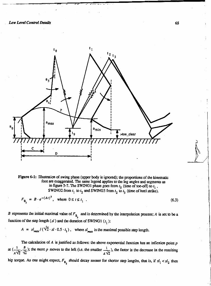
Low Level Control Details
Figure 6-1: Illustration of swing phase (upper body is ignored); the proportions of the kinematic foot are exaggerated. The same legend applies to the leg angles and segments as
in figure 5-7. The SWINGl phase goes fiom to (time of toe-off) to tl , SWING2 from tl to t2 and SWING3 fiom t2 to t3 (time of heel strike).
B represents the initiaI maximal value of F and is determined by the interpolation process; A is set to be a (33
fmction of the step length (sl ) and the duration of SWINGl (tl ):
A = sl- /(& - sl -0.5 . t1 ) , where sl- is the maximal possible step length.
The calculation of A is justified as follows: the h e exponential function has an inflexion point p 1 B 1 at (-+, ;E ); the more p moves to the left (i.e. the smaller ), the faster is the decrease in the resulting
A 2 A 3
hip torque. As one might enpen, F should decay sooner for shorter step lengths, that is, if sll < s12 then O3

Low Level Control Derails 66
. On the other hand, the inflexion point should never occur too late to maintain a rapid decmse
in F relative to the time tl for SWING1. After experimentation with the system, it was found that the most 83
natural motion resulted if the limit put on p was half the time for the SWINGl phase (i.e.
During a human locomotion cycle, the extension moment at the hip of the swing leg starts in the
double support phase and produces a continuous motion at toe-off. Equation (6.3) implies, however, that the
hip torque sets in suddenly with a maximum value at the beginning of the SWINGl phase., there is no hip
torque during the double support for the impending swing leg since its motion is completely expressed by the
kinematics of the virtual leg concept To assume a smooth msition at toe-off, the equations of motion for
the SWING1 phase have to be initialized properly with the leg angles and angular velocities at the hip from
the end of the meta-off period. The velocities are calculated simply from
e'j(t0)-e3(t0-At) e3 = , where At is the time increment.
At
While the hip torque drives the thigh to its desired orientation at the end of the SWING1 phase, the
ankle moves along the 4th order polynomial curve
where x and y are the coordinates of the ankle; the evaluation of the coefficients Ai is delayed for a moment,
in order to fiiish the discussion of the joint torques for SWING1. One method to constrain the ankle to the
curve P during SWING1 involves the application of a knee torque F . Since a moment produced at the 94
knee affects the hip angle as well, this approach could be difficult to implement. Instead, a simpler method is
employed, which totally eliminates the need for controlling a knee torque: the knee joint is locked for the
dynamics. At each time step in the simulation, the knee angle is updated kinematically such that the
constraint on the ankle motion is satisfied (i.e. the ankle lies on P). This updated position of the ankle, that is
the new value for e4 is used for the dynamic simulation at the next time step. To account for the locking of
the knee, the equations of motion (see appendix C.2) are modified as follows, assuming the matrix
representation:
b; = ,!$ = 0 , d4,4 = 1 and a'2,4 = = 0 .

Low Level Control Details 67
The knee angle e4 at each time step is calculated from the three equations shown below; the hip
angle €I3 comes from the dynamics of the swing leg and the position of the hip (xh,yh ) is known from the
stance phase simulation. The three unknowns are e4, x and y ; the latter two define the ankle position:
f , ( ~ , y , 9 ~ ) = xh - l,sin9, - 14sin(93+94) - x = 0
f2(x,yse4) = yh - I3cosg3 - I4co~(g3+e4) - y = 0
f3(sy,9,) = A0x4 + A,X? + + A3x + A4 - y = 0 .
The values of x and y from f, and f2, respectively, are now substituted into f3, which is solved for 04.
Unfortunately, there is no analytical solution. Therefore, numerical interpolation techniques are applied. The
Bisection method is used to compute a good first approximation, which is subsequently refhed by the
Newton Raphson method [Burden 851. Initial lower and upper bounds on O4 (which correspond to an ankle
position ( x g ) above and below the polynomial P) are obtained by an algorithm similar to (4.5). The
Newton-Raphson method converges fast, usually within 3 or 4 iterations; it can be used in this case because
the first derivative of f3 with respect to O4 exists:
f; = (4A0X? + 3 ~ ~ 2 + A2x + ~ ) - ( - ~ ) ~ o s ( 9 ~ + 9 ~ ) - 14~in(83+94) .
So far, the calculation of the hip and knee angle has been discussed. The two remaining leg angles of
the ankle and meta joint am determined by linear interpolation between the values at lopoff (time to ) and
the end of SWINGl (tl ). Whereas the former are known from the end of the kinematic meta-off phase, the
latter are specified as locomotion attributesE (swingl-ankle , swingl-me t a). However, the toe might
stub the ground in the event of a flat shape of the polynomial P (if a- is small, see figure 6-1). This is
prevented by a constant checking for ground contact during SWING1 and if need be, the ankle is dorsiflexed
temporarily just enough for toe-clearance.

Low Level Control Details
The derivation of the P as defined in equation (6.5) is now described. In order to compute the
coefficients A. - A4 -which is done by a Gaussian elimination algorithm- five conditions for the motion of
the ankle are required. The following conditions, which are illustrated in figure 61 , establish a desirable
shape for P :
1. y(0) = a o
2. y(C) = a-
3. y'(C) = 0
The horizontal position of the ankle at toe-off is assumed to be zero; a. is computed at the end of the
previous meta-off period. At a distance C, the ankle reaches a maximum height a- during swing. Based
on observations by Beckett and Chang [Beckett 681 and Inman [Inman 811, C amounts to about 30 % of the
value for D (see below). A locomotion attributeE was defined to allow for adjustments. An upper bound on
is set to be l5 + 16, which is the length of the toe plus the mid-foot. The actual maximum height for the
current step in a locomotion sequence is expressed as a function of the minimum length omi, of the dynamic
stance leg for that step (this corresponds to a maximum knee flexion). This is justified by the fact that the
faster a person walks, the bigger the knee flexion during stance, which causes a lower ankle path of the swing
leg. Therefore,
- @min a- - - (I5 + 16) , where ll is the length of the extended leg. '1
At the end of the SWING1 phase (at tl ) the ankle arrives at a distance D and assumes the minimal vertical
value a- . By Ohis time, the hip angle has reached e3 d, for heel strike and the toe is exactly under the - knee. Since the position of the hip is determined by the stance leg and the ankle and meta angles are known
as well (swingl-ankle, swingl-meta), the values for amin and D can be readily obtained by
trigonometric calculations (note that both are functions of the step length, because they depend on e3 des ). - Nevertheless, particularly at short step lengths, there is a possibility that the computed value for ah turns
out to be too small so that the toe would go through the ground at tl or at least the toe-clear constraint
(specified by a locomotion attribute) might be violated. In either case, the hip angle is increased just enough
(€I3 clear) to satisfy the toe-clear constraint. This is the reason why the extension of the hip can get - bigger at tl than at heel strike, which can also be observed in real human walking at short step lengths. Of
course, for the calculation of D , e3 - rather than $ dcs is used. Conditions (3) and (5) above ensure the -

Low Level Control Detaikr 69
maximum and minimum criteria of P by setting the fust derivatives to zero at C and D . The resulting curve
will take on different shapes depending on the characteristics of the current walking step.
There is one more significant aspect about the SWING1 phase. If the initial estimate of the hip
torque B in equation (6.3) is very large, it might happen that the hip extends so much during SWINGl that
the ankle can not be "placedn on the polynomial P, no matter what knee angle O4 is chosen; in this case, a
recovery mechanism aborts the simulation of the current SWING1 phase, lowers the vdue of B and restarts
the interpolation ptocess.
During the SWING2 phase from tl to t2 (see figure 6-1) the thigh remains at a fairly constant
position, whereas the shank swings rapidly forward The dynamic simulation is based on the equations of
motion as formulated in appendix C.2 (which implies that the knee is not locked any longer). To move the
shank forward, a torque at the knee, FB , is calculated by interpolation (as introduced in section 4.5) in such a 4
way that the knee extends exactly at time t2 (a final knee angle bigger than zero may actually be selected by
a locomotion attribute, which was discussed in section 5.2); F thereby assumes the same exponential '34
profile as Fe during SWINGl defined in equation (6.3). This produces a quick decay for the knee torque, 3
and results in an acceleration of the shank at the beginning of SWING2 and a gentle extension of the knee at
the end In order to sustain a continuity in the motion of the shank across the phase change at t l , the
SWING2 phase is initialized with the value of the angular velocity F. at the end of SWINGl, which is @4
calculated from an equation similar to equation (6.4) (note that it is not determined by the dynamics since the
knee was locked during S WINGI).
Simultaneous with the knee moment, a hip torque F is applied throughout SWING2 to hold the '4 thigh in its desired position. The magnitude of this torque at each time step is defined as
F = 5 ( 9321ear - '3 - '3 '3 3
'33
where 4 represents a spring, v3 a damping constant; O3 and 83 are the current hip angle and angular velocity
at the hip of the swing leg. 03'3_clem is initially set to 83 & . . However, the foot might intersect with the - ground while the knee is extending. This could result from k3 and v3 being chosen too small, or by an
accentuated pelvic list (see section 5.3) and a short step length. To recover from this situation, a new
increased hip angle is defined such that the foot is lifted just above the ground at the time step where the
undesired impact occurred and the simulation of the SWING2 phase is then repeated with O3 ,!,,, - set to the

Low Level Control Details 70
new hip angle. Even with the new value for 03-CIcor which produces a larger F and therefore a greater 63
extension of the hip, it is possible for the foot to strike the ground again at a later time in the same SWING2
phase. Thus, the recovery measure might be applied several times. As the shank swings forward the foot
reaches its lowest point in the rotation around the knee when the ankle passes through the vertical.
Consequently, if O3 > e3 dcs , the algorithm attempts to reduce the hip angle to its desired value. The - - recovery and reduction measures are necessary to successfully generate SWING2 phases for different
locomotion parameten and attributes. They also guarantee a low position of the foot during the latter part of
the swing, which naturally occurs in a real human walk. Because of the feedback mechanism (i.e. the check
for impact), this approach might very well be modified to account for clearance of small obstacles along the
locomotion path.
As in the SWING1 phase, the angles for the ankle and meta joint during the SWING2 and
subsequently the SWING3 phase are determined by linear interpolation between the initial angles
(swingl-ankle, swingl-meta) at time tl and the fmal angles at heel strike at t3 . Whereas the meta
angle at t3 is assumed to be zero, the ankle angle is specified by a locomotion attribute as described in section
The SWING3 phase takes up the short period (by default 15 % of twiw ) at the end of the swing 4 .-
which is characterized by very little rotational movement at the joints of the swing leg (see figure 6-1, t2 to
t3) . Since the leg is extended and the knee is locked, the equations of motion are modified as in the
SWING1 phase; the dynamic model of the swing leg is now defmed as a single pendulum. To account for the
impulse as a result of the knee extension at the end of SWING2, the equations are initialized according to the
calculations in appendix C.3.2.
A constant torque is applied to the hip during SWING3 to bring about heel strike at exactly the time
for the end of the swing. This is achieved by the interpolation process described in section 4.5. Usually, the
hip torque takes on values to solely hold the leg in its position (and therefore its magnitude is similar to F 03
near the end of the SWING2, neglecting the rather minor compensation for the hee extension impulse),
while forward motion of the hip directed by the stance leg is mainly responsible for bringing the heel down
onto the ground. At heel strike, the orientation of the swing leg plus the impact conditions (see appendix C
3.1) are used to initialize the stance leg model for the subsequent stance phase.

Low Level Control Details 71
62.4. starting and Stopping
The subphases for the stance and swing described above apply not only during the rhythmic period
of a locomotion sequence, but also during accelerated and decelerated motion. If the locomotion parameters
change at any time during a walk, the different timing constraints and final conditions for the subphases
become active as soon as the current step is completed. However, for the first and last step the swing
subphases need to be adjusted to account for a different motion pattern of the leg.
M e n starting a walk from rest with both feet parallel on the ground, the SWING1 phase can not be
executed as discussed in section 6.2.1. Instead, the following algorithm is employed, which is based on the
same principle as the original SWING1 phase (i.e. the knee is locked for the dynamic simulation and the knee
angle is updated kinematically while a hip torque produces a forward swing of the thigh to its desired
orientation e3 d, ): rather than prescribing the motion of the ankle by a polynomial, the tip of the toe is lifted - up vertically. If the hip angle has not reached e3 d, by the time when the knee is directly over the toe (this - happens automatically by increasing the hip angle and moving the toe straight up), the toe holds its position
directly under the knee until the end of SWING1. The SWING2 phase can then proceed as usual.
On the last step, the SWINGl phase is applied normally except that the desired angle for the hip
03-dLp is not zero as one might expect, but calculated such that the knee of the swing leg at the end of
SWINGl is exactly at the same horizontal position as the toe of the stance leg (of course, the toe of the swing
leg is directly under the knee at this moment). In place of the SWING2 and SWING3 phases, the foot is now
just lowered straight down until it is flat on the ground parallel to the stance foot at the end of the swing. This
is implemented as sort of a SWING 1 phase by locking the knee for the dynamics and applying a hip torque to
arrive at a 7ao hip angle at twin* . Because the lowering of the foot takes place much more quickly than the
usual STANCE2 and STANCE3 phases, the duration is reduced to half the normal time; at the same time the
duration for the SWINGl phase is increased to satisfy tming .
It is noted that the algorithms for the fmt and last step of a locomotion sequence have been chosen
somewhat arbitrarily. Since no experimental kinematic data could be found in the literature on how human
beings start and stop a walk, the steps taken above are solely justified by our own observations. Also, a
compromise was made between generating a realistic appearance and controlling the dynamics.

Results
Chapter 7
Results
' . I . ,
- I . -
Figure 7-1: Display of a walking figure.
The KLAW &eyfrarne&ess Animation of walking) system has been implement& to animate
bipedal walking. It consists of two C-program modules, walk and walkdsp. Thc former does all the
calculations discussed in the previous sections, whereas the latter was written for displaying the results (i.e. a
walking figure such as that shown in figure 7-1) on an IRIS 2400 workstation. Appendix B.2 shows the
. interface between the two programs. The computation of all the body angles is time-consuming: for instance,
it took 31 see of CPU time on a SUN3-50 computer with floating point processor (Motorola MC68881) to
comptite the animated walk illustrated in figure 7-1 (5.57 see = 168 frames ). In practice, the SWING2
phase has been most expensive because of its recovery and reduction measures (see section 6.2.2); although
the duration of SWING2 is only about 35 % of the time for the swing, the simulation usually takes more time
than for the SWING1 and SWING3 phases combined.
72

Results 73
Some of the results of the walking algorithm are now discussed in more detail. The convention is
used that positive angles mean a flexion and negative angles denote an extension of a joint; for the ankle and
meta joint, a positive angle is a plantarflexion, whereas a negative value is a dorsiflexion. Except for figure
7-10, the ordinate values for all diagrams start at heel-strike (i.e. the motion of the left leg in figure 5-1 is
presented). All the joint rotations are assumed to be in the sagittal plane, that is, along the line of progression.
walking cyde (%) walking cycle (%)
Figure 7-2: Comparison of hip angles during a locomotion cycle. Left angles as calculated by KLAW, right angles obtained from a walking human subject Winter 793.
Figures 7-2,7-3 and 7-4 show the hip, knee and ankle angles as calculated by the walking algorithm
compared to real walking data collected by Winter [winter 791 for one rhythmic walking cycle (denoted as
W for further reference). The locomotion parameters for the "film" walk are approximately v = 5 h l h ,
sl= 0.79 m and sf= 107 stepslmin based on a body height of 1.8 m. Specifying a desired velocity of
v = 5 kmlh , the walking algorithm calculated (see appendix D) a "natural" step length sl = 0.77 m and a step
frequency sf= 107.5 stepslmin , which are very close to the real walk. Illustrations of both walks are given
in appendix F (figure F- 1 and F-2).
Since filtering and smoothing techniques were applied to the real walking data [Winter 791, these
angles produce more continuous curves. A peak occurs in the calculated KLAW hip angle (maximum
flexion) at around 40 9% into the cycle. At the same time the knee angle is a minimum, which means that the

Results
Figure 7-3: Comparison of knee angles during a locomotion cycle. LA: angles as calculated by KLAW; right angles obtained from a walking human subject [Winm 791.
walking cyde (%) walking cyde (%)
Figure 7-4: Comparison of ankle angles during a locomotion cycle. Left: angles as calculated by KLAW, right angles obtained from a walking human subject [Winter 791.

Results 75
leg is fully lengthened. The peaks signal that the leg extends too fast, which is caused by a quickly increasing
leg axis force Fa, that reaches a maximum at 40 % of the cycle time (see figure 7-7). Possibly an earlier
activation of the STANCE3 phase (set to start at the end of the SWING1 phase as defmed in section 6.1, in
this case about 35 % of the cycle), or a smaller value for e-i, could alleviate the problem. The relatively
flat shape of the KLAW knee angle curve during stance from about 10-30 % of the cycle is produced by a
stiff dynamic leg spring. A lower spring constant k, can help to more closely match the knee angle of the
real walk The magnitude of the KLAW ankle plantarflexion at the end of the double support phase, i.e. at
tocoff (60 % of the cycle), is significantly larger than for the "film" ankle. This is not unnatural, as
experimental data Fman 811 show similarly large values (between 20 and 30 ) at comparable walking
speeds. It should be noted that the deviations of the KLAW angles from the "film" angles are quite minor
and hardly visible in an animation of a human figure. Furthermore, the measurements of articulated motion
are not free of noise, and it is difficult to obtain simultaneous data of motion in all three reference planes
(sagittal, coronal and transverse). The walking algorithm, on the other hand, includes motions such as pelvis
rotation, pelvic list and lateral displacement of the body, which are only indirectly represented in figure 7-2,
7-3 and 7-4 (see also figure 7-12).
walking cyde (%)
Figure 7-5: Dynamic hip angle for walking cycle W.
Figure 7-5 shows the very regular behavior of the dynamic hip angle el over the duration of two
rhythmic walking steps: the angle increases from -25 " at heel strike to 25 " at the heel strike of the other leg.

Results 76
Towards the end of a step (40-50 % of the cycle), the curve bends upwards slightly, which represents an
increase in the angular velocity. This corresponds to an acceleration of the center of mass as discussed in
section 5.3.
- . - I . , . , - , - ,
0 20 4 0 60 8 0 100
walking cyde (%)
Figure 7-6: Upper body angle O2 (sagittal plane) for walking cycle W; a positive value corresponds to a forward tipping of the body.
In figure 7-6, the upper body angle €I2 is displayed as calculated by the dynamics. Shortly after heel
strike (at 0 % and 50 %) of the walking cycle, the upper body tilts forward as a result of the impulse.
However, the net change in the upper body angle is very small.
Figure 7-7 shows the leg axis force Fa and the leg torque F, during stance. The dynamic stance 1
phase for a leg ends with each step, since the other leg takes over at heel strike. Therefore the force and
torque pattern repeat with each step (this holds also for the swing phase torques illustrated in figure 7-8). F, 1
follows a regular pattern; as described in section 6.1, it acts as a step input torque for about 20 % of the cycle
time during a walking step. The value for Fa never drops down to zero, which means that the SWING2
phase was not activated (i.e. the leg was never locked) and STANCE4 had to occur just at heel saike of the
other leg. Shortly after heel strike, Fa increases to account for the impulse, which is achieved by an internal
increment in the position actuator pal . The end of the SWING1 phase is reached at about 35 % of the cycle,
which causes another temporary increase in Fa when STANCE3 sets in to lengthen the dynamic leg to its
desired value a,, at heel strike.

walking cyde (%)
Figure 7-7: Leg force F, and torque F during stance for walking cycle W. 01
Figure 7-8 illustrates the torques at the swing leg. A knee torque F develops only during SWING2 / \- 04
from 35 % until about 48 % of the cycle for the first step; it sets in with a maximum (negative extension)
magnitude and decreases according to the exponential function in equation (6.3). F follows the same 03
pattern during SWlNG1, from about 12 % (after double support with the beginning of the swing phase) until
35 % of the cycle time. In the SWING2 phase, the magnitude of F is determined by a spring and damping 4 construct, which causes irregularities in the profile particularly at the phase change from SWING1 to
SWING2 (see at about 80 % of the cycle time, where F actually becomes positive, which indicates a 03
flexion moment). The irregular behavior of F is caused by the sudden extension torque at the knee, which O3
has to be compensated in order to keep the hip angle constant.
Figure 7-9 displays the motion of one leg for a complete walk (including starting and stopping). The
. sinusoidal path of the hip (i.e. the vertical displacement of the center of mass) is more pronounced for the
faster walk during the rhythmic period, which is in accord with observations by Inman m a n 811 on real
human walks. The diagrams of figure 7-10 show the leg angles at each frame for the same walking sequence
(for the same leg). It can be seen that the maximum flexions of the hip, ankle and meta joints (ankle and meta
joint plantarflex) at toe-off are bigger during the second cycle, where the full velocity of 5 kmlh is reached,

Results
walking cyde (%)
Figure 7-8: Hip torque F and knee torque F during swing for walking cycle W. O3 '4
than in the first and third cycle, which are characterized by acceleration and deceleration, respectively. Only
the maximum knee angle stays fairly constant in all three cycles. This is in conformity with studies on real
human walking nnman 811 (see also the discussion of the meta-off phase, section 5.4). (It is noted, that the
walking sequence of figure 7-9, bottom, and 7-10 is also printed on the right margin of this write-up in
reverse order.)
A comparison of hip and knee angles for 3 walks with different step length and step frequencies, but
the same speed, is given in figure 7-11 over the duration of one rhythmic walking cycle. Photographic
Images of the same walks are presented in appendix F (see figure F-2, F-3 and F-4). An analysis is left to the
reader.
Figure 7-12 illustrates the effect of pelvic list in the coronal plane on the leg angles in the sagittal
. plane. Between 40 % and 70 % of the walking cycle, the hip joint of the walk with an accentuated pelvic list
(3-3) does not flex as much as the hip joint during a normal walk (3-1). In other words, the bigger the pelvic
list, the more the thigh of the hind leg extends forward towards the end of the double support phase. Of
course, at heel strike, both the hip and the knee angles must be the same because the walks are based on the
same locomotion parameters. The knee flexion of (3-3) is increased from about 55 % to 75 % of the cycle
compared to (3-1) to account for the lower hip position.

Results
Figure 7-9: Motion of leg for two complete walking sequences at different speeds (only one leg is displayed). Both walks cover about the same distance from the start to the end. Top: 2 kmlh ,204 frames, 4 walking cycles (2nd and 3rd cycles are rhythmic).
Bottom: 5 kmlh , 108 frames, 3 walking cycles (2nd cycle is rhythmic).

0 2 0 4 0 6 0 80 100 120
frame #
frame # frame#
Figure 7-10: Hip, knee, ankle and meta angles for a complete waking sequence (including starting and stopping) of 108 frames, which corresponds to the walk of figure 7-9, bottom.

Results
frame #
f rame #
Figure 7-11: Hip and knee angles for 3 walks with the same speed, v = 5 kmlh, but different step lengths ( ~ 1 ~ - ~ = 0.5 m , slw = 0.77 m and s15-, = 1.05 m ) and different step frequencies
(g5-l = 166.7 stepslmin , .fw. = 107.5 stepslmin and sfs2 = 79.4 stepslmin). The number of frames for each wallung cycle w are: wS1 = 23, wg4 = 34 and = 46.
Walk 5-0 is a "natural" walk.

Results 82
walking cycle (%)
walking cyde (%)
Figure 7-12: Hip and knee angles of 2 walks with the same locomotion parameters ( v = 3 kmlh , sf = 0.6 m and@=83.3steps/min),butadifferentvalueforthepelvic-list factorlocom~tion
attribute: pe lv ic- l i s t - factor = 1 , pe lv ic- l i s t - factor = 3 . A rhythmic wallung cycle is assumed.

Conclusions 83
Chapter 8
Conclusions
The principal objective of this thesis was to design a control algorithm for the animation of bipedal
locomotion. The KLAW sy&m which has been implemented can generate a large variety of walking
sequences and the two sub-goals of developing a high-level control scheme and producing realistic motions
have been successfully translated into action. A natural animation of a walking human figure is obtained by a
hierarchical decomposition of a task specified by a few waking parameters. The decomposition is achieved
by combining several motion control techniques in an elegant way, eliminating a lot of the disadvantages that
occur in the separate application of,any one of these techniques (as described in chapter 2).
It has been shown that a simple dynamic model is sufficient to simulate a generic locomotion
pattern. The effects of gravity, ground collisions and active muscle moments during a human walking cycle
are adequately accounted for by the sys.tem. The simplicity of the dynamic model makes it possible to
determine the governing forces and torques based on internal knowledge and rules about locomotion. This 1: eliminates a major problem attached to applying traditional forward dynamics to computer animation: rather
than having to specify the cause of a motion in terms of forces and torques, the user can select a number of
more obvious motion parameters such as velocity and step length. From a hierarchical viewpoint, the
equations of motion provide the low-level, natural execution of the leg movements. They symbolize the
functional synergies that are controlled by the motor program for wallring as discussed in section 3.2. The
motor programs embody the rules about a locbmotion cycle, which are incorporated at several levels in the
motion control hierarchy. High-level concepts such as step-symmetry and state-phase timings define the
boundary conditions for a specific walking configuration. Rules at the middle level govern the coordination
of the legs; this involves the proper sequencing of the leg-phases. At the bottom level, knowledge about
walking leads to a subdivision of the original phases and the calculation of the force and torque profiles.
Kinematic rules about the motion of the foot, leg, pelvis and upper body are integrated into the dynamic
simulation.
Goal-directed and dynamic approaches to motion control have been tied together in this thesis.
Although the implementation was done specifically for bipedal walking, we believe that the basic ideas can

be extended and applied to other forms of articulated motion as well. In practical terms, the dynamics could
be regarded as an interpolation method berween the key frames defined by some high level concepts (in this
case, step symmetry and state-phase timings). Therefore, the ultimate goal is to built an entire animation
system for articulated figures, where different classes of motions (locomotion, grasping, standing up, turning,
etc.) are implemented as tasks which the animator can activate by a few motion parameters (see also figure
3-2 (b)). The usefulness of such a system would greatly depend on the choice of parameters assigned to each
task.
The KLAW system developed in this thesis can be integrated into current animation systems to
produce sequences of walking. For instance, in a keyframing system such as the V-2000 system of Vertigo,
an initial and final key position of a figure could be specified and the KLAW system would then generate a
walk in-between. Some of the extensions mentioned below (e.g. the possibility of changing directions)
would be necessary to make this symbiosis more practical.
&
A direct extension of the algorithm would be the inclusion of other bipedal gaits and locomotion
with more than two legs. Suggestions are given in sections 3.2,5.1 and 5.2. Whereas running, for example,
would require a modification of the dynamic model to account for the flight phase during which both legs are
off the ground, additional legs are merely a coordination problem at the "state" level. The algorithm was
designed for legged locomotion on level ground. However, we think that walking up and down inclines and ! stairs could be implemented in a straightforward manner based on the same principles. For instance, walking
up stairs would involve the definition of a new local motor program (see figure 3-2) for the swing phase,
whereby the feedback mechanism for foot clearance (discussed in section 6.2.2) could be adapted to move
the leg from step to step; for walking downhill, a greater knee flexion during stance would have to be
accounted for in the local motor program for the stance leg by reducing the stiffness of the dynamic leg
The usability of the algorithm could be improved by a better user interface, where the locomotion
parameters (i.e. velocity, step lengthand step frequency) and possibly the locomotion attributesE would be
specified and modified interactively as functions of time. In the current version of KLAW, it is only possible
to generate walks with an acceleration period at the beginning and a deceleration at the end of the locomotion
sequence. By adding functions for the direction of locomotion, KLAW could be interfaced with path-
planning algorithms. A change in direction could be implemented by adding "kinematic" degrees of freedom
(as in the case of the legdeterminants) to enable the legs to swing slightly sideways.

Is is also desirable to make the algorithm more efficient in order to come close to real-time
A significant speed-up could be expected if a faster integration method was used (the
LSODI [Hindmarsh 801 FORTRAN routine does a lot of extra, time consuming checking). Also, it would be
worthwhile to examine the numerous trigonometric expressions used in calculating the kinematic gait-
&terminants for a more efficient fonnulation.

Terminology
Appendix A
Terminology
The following is an alphabetically ordered list of frequently used terms from Computer Animation,
Physics and Artificial Intelligence. They are explained or defined in the way in which they are used in the
context of this thesis.
Animtion This literally means 'to bring to life'; it is the process of representing changes of movements over
time. Generally, the motion is generated through the rapid display of successive images, fast enough (24
frames/sec for film, 30 frames/sec for video), that the human eye interprets them as continuous motion.
Originally, animation was restricted to 2-D (Walt Disney, Warner Brothers) or 2%D (pictures are drawn on
parallel planes, that can be moved against each other).
When computer technology was ready to be applied to animation, it first served mainly as an
assisting tool. The computer supported color drawings, the calculation of in-betweens and film-recording.
Today, 3-D computer animation is common practice and is an entirely different medium. Often
termed modeled animation, it supplies the animator with a whole new set of tools for the modeling-
animating-rendering procesS. 3-D models, color, shading, movement of camera (viewpoint) and other
techniques greatly enhance realism.
. Articulated Body The body is made up of segments or links (usually rigid) connected by joints. The motion of the
segments relative to each other is somewhat restricted. The human body is expressed as such an articulated
body. It can be represented as a aee structure (transformation tree) where the segments (joints) are taken as
nodes connected by joints (segments). Each node has its own coordinate system (transformation matrix).

Nodes located more deeply in the tree will be transformed by matrices from ancestor nodes, when the tree is
mversed, e.g. a wrist-node gets transformed by the elbow-node above it, if the lower arm is moved.
Each joint has one to three rotational DOF (up to two degrees of constraints). Joints with 1 DOF are
called hinges (e.g. elbow), with 2 DOF they are called universal joints (e.g. finger) and with 3 DOF, joints
are referred to as ball joints (e.g. shoulder). The total number of DOF of the body is the sum of the DOF at
each joint plus the 6 DOF of an initial joint (position and orientation of the body as a whole) which
"connects" the body to the world.
Center of Mass Traditionally, the center of mass of a system is defined as the sum of the products of all its particle
masses and the distance from the origin divided by the total mass of the system. With articulated bodies, the &
calculation of the center of mass is simplified, since the mass of each segment can be expressed as a function
fi. of the total mass M (e.g. thighbody= 0.1, total arrn/body= 0.05). The center of mass x therefore is:
In locomotion of articulated bodies the center of mass constantly changes, so it has to be recalculated
for each time-step. It plays an important role in balancing the body.
Conservative System In this context, a physical system (e.g. a double pendulum) is conservative, if no external forces and
torques are acting on it except gravity. An exact definition is given below.
If the work done by a force in moving an object from one position to another only depends on these
two positions but not on the path followed, the force is said to be conservative and the system is referred to as
. a conservative system. For example, if a block is raised from the ground to a height h, the work done on the
block by the gravitational force is mgh. Since there is no work by gravity in the horizontal direction, the
work done on the block to lift it to height h remains the same, whether it is moved up vertically in a straight
line, zig-zag or along any arbitrary path. Hence, gravity is a conservative force and, if air resistance is
the system is conservative. But if the block is pushed horizontally on a table from A to B, the work
on the block is done against a fictional force, which is always directed opposite to the motion. Now the
amount of work depends on the path taken between A and 8 , in that the longer the path is, the more work has
to be done. In this case, the system is non-conservative and friction represents a non-conservative force.
Degrees of Constraint A single particle in space has 3 DOF. If its motion is restricted to a line 01 = ax + b , z = O), one
coordinate is sufficient. The particle is said to have 2 degrees of constraint and therefore only 1 DOF.
Degrees of Freedom (DOF) 'DOF are the number of independent parameters (not including time) required to completely specify
the position of every part of the system. For example, a single particle has 3 DOF in space, a segment or
rigid body has 6 DOF (3 translational coordinates for position and 3 rotational ones for orientation), a double
pendulum with moving reference point free to move in space has 9 DOF (3 translational coordinates for
position and 6 rotational ones for orientation).
Differential Equations of Motion Dynamic analysis of a system involves expressing its behavior over time. For example, if we have a
particle of mass m fastened to a spring with force constant k, and the displacement of the particle is x , then
the behavior of this system is formulated as
m x + k % = O ,
which is derived from Newton's 2nd law of motion, F= ma by letting F= -kx (Hooke's law) and a = x, the
2nd derivative of the displacement over time.
The above equation is called the differential equation of motion for the system, which can be set up
in various ways (Lagrange, Newton, D'Alembert, Hamilton ) [Wells 671. Except in the Hamiltonian fom,
they are all of 2nd order.
In this simple case, only one coordinate (displacement in x-direction) is considered. Usually, in

Tennino~ogy 89
particular when dealing with articulated bodies, the number of DOF is large, thus resulting in many equations
of motion, since there is one equation for each DOF. Because the equations are non-linear, complex and
coupled most of the time, a solution (to the direct dynamics problemA) can only be found by numerical
methods.
Duty Factor The duty factor of a foot is the fraction of the duration of the stride for which this foot is on the
ground.
Dynamics This is the study of changes in motion due to forces and torques. In Biomechanics Winter 791, this
discipline is often called kinetics. Considering the human body, internal forces (caused by muscular activity,
ligaments, frictions in musdes and joints) as well as external forces (ground reaction forces, collisions with
active and passive bodies) have an influence on movement. Classical dynamics is based on Newton's 3 laws
of motion. Equations of motion can be solved in 2 directions:
direct (forward) dynamics problem given the forces and torques, solve for the accelerations, i.e. determine the resulting motion of the system. In Computer Animation, dynamics is usually applied in this form.
inverse dynamics problem given the motion of a system (i.e. the accelerations), solve for the forces and torques that produce these accelerations. In Biomechanics, one often has to resort to this approach, since the measurements of forces and torques (which have to be known for direct dynamics to be applied) are mostly inaccurate and difficult, if not impossible, to measure. On the other hand, positional data (i.e. accelerations) can be readily gathered. Thus, via inv- dynamics, the forces and torques can be calculated.
\
Frames A frame-based representation scheme specifies a knowledge bas&, which is a collection of frames
logically connected and organized in some (mostly) hierarchical manner. A frame winsky 751 is a data
structure for representing stereotypical situations, such as being in a certain kind of living room or going to a
child's birthday party. The salient idea behind this is to group pieces of knowledge into microworlds, which
may be useful for understanding a particular concept. Each frame has terminals or slots for attaching pointers

to substructures. Different frames can share slots, e.g. the frames for a table and a chair might share the slot
for a leg, if both have legs of the same geometrical nature. Terminals of a frame are usually stored with
"weakly" bound default assignments, which can be updated or replaced for a particular instance.
Gait Different styles of locomotion depend on speed and on the structure of the animal. Gaits can be
classified as walks and r m . Walks have duty factorsA 2 0.5 (for a certain time during a stride all feet are on
the ground), whereas runs have duty factors < 0.5 (there is a time during a stride when all feet are off the
ground). A gait is called symmetric, if the left and right feet of each pair have equal duty factors and relative
phasesA differing by 0.5 . Thus human walking is a symmetric gait. Also amble, trot and pace are symmetric;
gallop, hopping or canter are asymmetric [Alexander 841.
Kinematics This is the analysis or description of movements of bodies or parts of bodies in time and space
independent of the forces, that cause these movements [Wilhelms 85, Dagg 771. It involves the calculation of
linear and angular displacements, velocities and accelerations. The kinematics of articulated bodiesA results LL in the following two related problems:
direct Cfonvard) kinematics problem find the position of a distal segment of the body given the joint angles of the proximal segments, e.g. find the position of the foot given the angles of the hip, knee and ankle.
inverse kinematics problem find all the joint-angles of the proximal segments required to produce a particular absolute position of a distal segment, e.g. given the position of the foot, find the joint- angles at the ankle, knee, hip, which will place the foot at that position. Inverse kinematics finds applications in robotics, where, for instance, the robot hand has to be placed at a certain known position in order to grasp something; or in locomotion to place and hold a foot at a position on the ground, while the body is passing over it. With articulated bodies the inverse kinematics problem can be very difficult to solve [Girard 851.

Knowledge Base The central issue in knowledge representation is to fmd proper internal representations for expert
knowledge along with associated knowledge handling facilities to create intelligent systems.
The different notations for representing knowledge are referred to as representation schemes. By
making use of such a representation scheme, a knowledge base can be specified, which is basically a model
of the world containing various facts. There are different classes of representation schemes: logical, network,
procedural, frame-based, etc. Flylopoulos 831. A procedural representation scheme, for instance, can
specify a production system. The knowledge base would consist of a number of production rules and a
database. The production rules are of a "if pattern then action" type. If the pattern matches some fact in the
database, the action is executed.
~ o m e n t of Inertia See Radius of Gyration.
Particle An imaginary bit of matter (visually a dot), so small, that it is totally determined in space by 3
coordinates.
Radius of Gyration (y) L
The distance from any given axis of rotation, at which the mass of a rigid body could be
concentrated without changing the moment of inertia, I , about that axis of rotation. For the application here,
the moment of inertia about the center of mass, Io, is important. In this case, y is such that 2 equal point
masses (located at a distance y at either side of the center of mass) have the same moment of inertia as the
original distributed mass: 2 - m 2 m 2 Io=my --y +Ty
2
It should be noted that the moment of inertia about any other axis of rotation (usually the proximal or
distal end of a segment), which is parallel to the axis of Io, can be determined by applying the Parallel Axis
Theorem Winter 791:

where x is the distance between the center of rotation and the center of mass.
Relative Phase The setting down of a foot with respect to the setting down of an arbitrary chosen reference foot,
expressed as a firaction of the duration of the stride. The reference foot is assigned relative phase 0 and the
others have relative phases in the range 0- 1. Alexander [Alexander 841 presents various examples.
Rigid Body Defined by a number of points, that must move together as a whole; they may not move relative to
each other.
Simulation Ib In this context, simulation is defined as the process of studying the behavior of a physical system 4
under various conditions using a computer model. A model is an internal representation of a system where
mathematical equations define its components and their interactions IJAiller 751. The graphics is completely
decoupled from the model. In simulation as opposed to animation, a system is described by governing
dynamical equations, whereas animation is fkquently associated with kinematics. Here, simulation is treated
as a particular animation technique, where motion control is determined by dynamic equations of motion.
Step During each stride for bipedals, there are 2 steps, one left and one right. A step is the movement of a
single leg from the time it is lifted off the ground until its next lift-off. A step is divided into stance and swing
phases.
Terminology
Stride Complete cycle of leg movements, e.g. from the setting down of a particular foot to the next setting
down of the same foot.

r
Body Data
Appendix B
Body Data
B.1. Anthropometric Data
The anhpometric data shown below are used for dynamic analysis and lower body kinematics,
respectively. It is claimed in this context that in determining the dynamics of the stance leg and the shank of
the swing leg, the segment weights, centers of mass and radii of gyrationA (moments of inertia) include the
physical properties of the foot. Data for the lengths of segments were drawn fiom various anatomy books, all
other measurements are bornwed fiom a book by Winter [Winter 793.
for segment i , 1 i = segment length I body height mi = segment weight I body mass r i = center of mass 1 segment length y i = radius of gyration A I segment length
upper body 1 m r y 2 2 2 2
pelvis thigh l3 m3
I b shank li
foot 1 5 1 6 171*19
Figure B-1: Indices for anthropometric values of lower body segments.

I i' i Body Data
Table B-1 lists the relative anthropometric data for each of the segments illustrated in figure B-1. It
should be noted, that except for rl , which is measured from the distal end, the centers of mass are given from
the proximal end of a segment. The radii of gyration are specified with respect to the center of mass:
I upper body 1 2 1 0.47 1 0.678 1 0.5 1 0.496 1
pelvis
leg 1 thiz 13 10.23669 1 o:L 10.:3 10.:3 1 4 0.24556 0.061 0.606 0.416
mid foot 5 0.0858
I toe 1610.04734( - I - I - I
0
1
Table B-1: Anthropometric values of lower body segments (the * indicates a vertical distance rather than a segment length).
The absolute anthropometric data, including the moments of inertia Zi, are calculated once the values
for body height and body mass are specified. As an example, if the total body height is to be 1.8m and the
body mass 75 kg, the following values result for the thigh:
0.10059
1 + 1
- 9 + m, 0.553 0.326

Body Data
B.2. Human Walking Figure Data
The following data structure is updated by the KLAW system for each frame (&c ) m animate a
human walking figure using a left-handed coordinate system. Rotations about the x, y, z axes are denoted by
the suffix -a, -ry, -rz , respectively.
type&f atruct {
float int int int int float float float float float f loat float float f loat float float float float
float float float float float
float float float f loat float float f lort float float
f loat float float float float float float float float f loat float f loat
walk-data
time; state; cyal.; rightghaae; leftghamo; body-tx; body-ty; body-t z; pelvia-ry; polvia-rx; right-hip-rz; right-knee-rz; right-ankle-rz; right-mrta-rz; le ft-hip-rz; left-knee-rz; loft-ankle-rz; loft-mota-rz;
/* currant ti- */ /* atde (ainglo or double support) */ /* cycle (&velop, rhythmic, decay) */ /* 1.g phaso (STANCE1,2,3,4; SWINC1,2,3 */
/* roferoncm poaition of the body */ /* (loortad halfway botween hipa) */
/* pdvic rotation /* pelvic list /* 8, /* o4 /* es /* 8,
/* diatribution of uppor body angle 8, */ " lumbarl-rz ; lumbar2-rz ; lumbar3-rz ; lumbar4-rz ; lumbar5-rz ;
/* distribution of compensation for */ /* pelvisrx */
right-hip-rx; right-ankle-rx; loft-hip-=; left-ankle-rx; lumbarl-rx; lumb8r2-rx; lhar3-rx; lumbar4-rx; lumbar5 -rx;
/* diatribution of comp.n~ation for */ /* pelvia-ry */
right-hip-ry ; left-hip--; lumbarl-ry ; lumbar2-ry; lumbar3-ry ; lumbar4-ry; lumbar5-ry; thoraxl-ry ; thorax2-ry; thorax3-ry; thorax4-ry; thorax5-ry;

Body Data
float float float f loat float f loat float float float float f loat float float float f loat f loat
f loat float float f loat
) WALKDATA;
thor-6-ry; thorax7-ry; thoru8-ry; thoru9-ry; thorul0-ry; thorurll-ry; thor.xl2-q; cmrviaall-ry ; cervical2-sy; crrvical3-ry; crrvical4-ry; cervicals-ry; cervical 6-ry ; cervical7-sy; righttahoulder-sy; lmft-ahoulderight-ry;
/* arm right-shoulder-rz; left-ahoulderight-r~; right-elbow-rz; left-elbow-rz;
97
awing
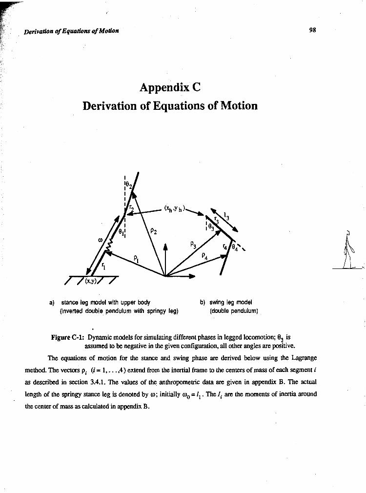
Appendix C
Derivation of Equations of Motion
a) stance leg model with upper body b) swing leg model (inverted double pendulum with springy leg) (double pendulum)
. Figure C-1: Dynamic models for simulating different phases in legged locomotion; O3 is
assumed to be negative in the given configuration, all other angles are positive.
The equations of motion for the stance and swing phase are derived below using the Lagrange
method. The vectors pi (i = 1, . . . ,4) extend from the inertial frame to the centers of mass of each segment i
. as described in section 3.4.1. The values of the anthropometric data are given in appendix B. The actual
length of the springy stance leg is denoted by o; initially oo = I * . The Ii are the moments of inertia around
the center of mass as calculated in appendix B.

p r >
Derivation of Equations of Motion
C.1. Stance Phase
The Lagrange equation for the stance phase can be written (see section 3.4.2) as
The kinetic energy of the system (see figure C-1 (a)) is expressed by
1 . 2 1 . 2 1 2 1 . 2 = - m pl + Tm2p2 + -I 6 + T1202 . Tst 2 1 2 1 1
where the squares of the translational velocities of the centers of mass 6: and b: are calculated as follows:
Since the foot remains fixed on the ground during stance, i.e. x = j; = ; = = 0, this reduces to
Similarly,
p2 = [ X + msinB1 + r2sine2, y + 0 c o s 8 ~ + r2cose21T
Therefore, the kinetic energy becomes
1 1 2 2 '2 1 2 .2 Tst = - m d, + 1(11 + mlrl + %o )e l + -(I + m2r2)$ 2 2 2 2
+ m2r292(081'ms(e2-01) - hsin(e2-e l ) ) .
The potential energy of the system amounts to .
Ust = mlg(y + r lcosel) + %g(y + ocosel + r2cose2) .
Substitution of Tst and Ust into equation (C.l) and differentiation with respect to o , and O2 leads to 3
equations of motion, which totally describe the system. Step by step,

Derivation of Equations of Motion

Derivation of Equations of Motion
After rewriting the equations in matrix form A & = B ( qst , qS>, they are transformed to a set of first
order equations (see section 3.4.3) of the form
A'ust = B' ( u s t ) , where

Derivation of Equaticrns of Motion
C.2. Swing Phase
The Lagrange equation for the swing phase can be written as
From figure C-1 (b) we derive (note that e3 is defmed to be negative for consistency)
p3 = [x, - r3sine3, yh - r 3 ~ s e 3 l T and
p4 = [xh - 13sine3 - r4sin(03+04)7 yh - l 3 w s q - r4~os (03+04) ]T .
Substituting
-2 -2 2 -2 i: = xh + yh + r3e3 - 2r303(4cos03 - jhsine3) and
6: = 4 + $ + r:e: + r:(e3+e4)2 - 2i34(i, ,cose3 - jhsine3)
- 2 r 4 ( e 3 + 8 4 ) ( ~ h ~ ~ ~ ( ~ 3 + 8 4 ) - &sin(e3+e4))
+ 2 l3 r4 e3 ( e3 + e4 ) COS e4
into
1 1 1 T, = i m 3 $ + ? m 4 i ; + -I 2 3 e2 3 + i~4(e3+e4)2
yields
1 -2 -2 1 2 2 -2 T, = T(m3 + m 4 ) ( ~ h + yh) + Z(13 + m3r3 + m413)e3
1 2 + -i(14 + m4r4)(63+04)2 - (m3r3 + m413)93(&~os03 - jhsinB3)
- m 4 r 4 ( e 3 + e 4 ) ( ~ h ~ ~ ~ ( e 3 + e 4 ) - jhsin(e3+e4))
+ m4 l3 r4 e3 ( e3 + e4 ) cos e4
for the kinetic energy. The potential energy for the swing phase is
Usw = m 3 g ( ~ h - r 3 c ~ ~ e 3 ) + m4g(yh - 4cose3 - r4c0s(e3+e4))
The two equations of motion can now be derived by differentiating the Lagrangian analogous to the stance
phase. This results in

Derivation of Equations of Motion 103
It should be noted that the translational motion of the hip of the swing leg does not impose additional
degrees of freedom to the system, since this motion is determined by the stance phase model as follows:
xh = x + Cosinel yh = y + WcoseI
Xh = Osin O1 + o 8, cos yh = OCOS el - o el sin el ih = tisin0, + 2 6 4 C O S B ~ yh = ti cos 0, - 2 i 6, sin el
+ 0(Zj~cos0~ - 9;sine1) - 0(Zj,sin0~ + 8 ~ c o s e 1 )
.. .. . . wherex=y=x=y=O .

Derivation of Equathns of Motion
After transformation to a set of k t order equations, the matrix formulation
A'L = B'(uw)
is expressed by
= r 03943,04;441T
-m3gr3 sin 03-m4g (I3 sin O3 +r4 sin (€I3 + €I4))
94
- 2 -m413 r4e3 sin 04-m4gr4sin($ +04)

Derivation of Equations of Motion
C.3. Collisions
C.3.1. Heel Strike
At impact (heel strike), the following calculations are done based on the conservation of linear and
angular momenta ( - means before, + after impact). For the angular momentum at the hip of the stance leg
With
r',= [r2sine2, r2cose21T and
p2 = [ i + &sine1 + a81cos81 + r2qcose2 ,
y + b ~ s e , - ~ 0 8 ~ s i n e ~ - r2$sine21T
and using the fact, that b = 0 before heel strike, i.e. there is no velocity along the leg axis in the air, and . . x = y = 0 after heel strike, since the (dynamic) foot does not move on the ground, we have
The angular momentum at the foot before and after impact is expressed by
+ L; = L; where Lf = 1~8, - r l x m l ~ l + 1~8, - p x m 2 p 2 .
For simplification, this can be written as
With p2 as defined above and \
T PI = [ r l sine1, rl cos 0, 1 ,
pl = [ i + r181cos01, y - r181sinel]T ,
3 = [as ine l + r2sine2, acosel + r2cose,] T
and again, w- = 0, x+ = = 0, this yields

Derivation of Equations of Motion
A third condition comes from the conservation of linear momentum along the leg axis,
For this purpose, the reaction force R is considered
. - RAt = m2(p; - h) , ~ith~~asdefinedabove.
Since for the instant at impact, there is no contribution of the force in the direction of the leg, it follows that
(RXAt)sin9, + (RYAt)cosel = 0 .
With cj'- = 0 and x+ = j;f = 0, this yields
J --...
It should be noted that i- and y- of the foot before impact as used above are determined as follows
from the swing leg:
where is the length of the swing leg after extension. The three equations (C.3), (C.4) and (C.5) can now
be solved for cj", 0:, 8; . \
C.3.2. Locking of the Knee
The value for the hip angle, 634, after the extension of the swing leg is calculated from the
conservation of angular momentum at the hip:
which can be expressed as

Derivation of Equations of Motion 107
1~8, + P 3 x m 3 p 3 + ~ ~ ( i ) ) + e ~ ) + d x m 4 p 4 = ~~~e~~ + 9 3 4 ~ m 3 4 p 3 4 , (C-6)
where
m3 '3 + (5 +',I "1,
'34 = * '"3+rn4
m3,= 9 + m 4 = ml and 134=11 .
Assuming e3 and 6, to be defined as in appendix C.2 and
t = [-13she3 - r 4 s i n ( e 3 + e 4 ) , -13cose3 - r 4 a w ( e 3 + e 4 ) l T ,
T p3, = [$ - r3, B,, cos e3, yh + r3, e3, sin e3 ] ,
equation (C.6) becomes
2 = ( 13, + m3, r3, ) $, + m3, r3, (x: cos e3 - j i sin e3 ) ,
from which e3, can readily be determined.
Derivation of Equations of Motion 108
C.4. Spring and Damping Constants
The following are the default values assigned to the various sping and damping consrants (ki, vi )
and position actuators described in chapter 6 (a body weight of 75 kg and the anthropornetdc &ta'in
appendix B are assumed).

Locomotion PamrneCers
Appendix D
Locomotion Parameters
The algorithm below calculates the non-specified walking parameters and/or verifies the specified
ones. The three walking parameters are velocity (v), step length (sl) and step frequency (sf). If a walking
parameter is zero below, it means that it is not specified.
if ( v >= v-Inax ! ! s1 >r 61-Inax ! ! sf >= sf-Inax ) /* reject, since walking is not poasible return;
if ( v != 0 ) /* velocity is specified */ {
if ( 81 != 0 LL sf != 0 ) /* velocity, step length and step frequency are specified */ {
if ( sf * 61 != v )
{ /* reject, since walking is not possible return;
1 1 else (
if ( s1 != 0 LL sf - 0 ) /* velocity and step length are specified
sf = V / s1; 1 else {
if ( 81 - 0 LL sf != 0 ) /* velocity and step frequency are specified {
s1 = v / sf; 1 else {
if ( s l = = = O L L s f = = O ) /* only velocity is specified * / {
sf = sqrt( v / ( body-height * 0.004 ) 1; if ( sf > sf-norm ) l
sf = v / 61-norm; 61 = 81-norm;
1 else (
s1 = v / sf; ) ) l l ) l
... continued on next page

Locometion Parameters
e l se /* volocity is not 8pecifi.d I
i f ( 61 != 0 LL s f != 0 ) /* stop longth m d s tep f r~quuray aro both given
/* roject, sin- walking is not possible return;
1 1 e l se f
i f ( s f - 0 LL s1 != 0 ) /* only s tep length is given f
i f ( 61 <= 81-norm ) f
sf = 61 / 1 olse f
i f ( s1 >
s f = sf *= s f +=
1 1 1 . e l se f
sl-norm LL 61 < el-max )
f 81
1 1 1 else f
' /* nothing return;
1 1 v = sl * s f ;
1 1
i f ( s f != 0 LL 61 0 ) /* only step frequency is f
i f ( s f <= sf-norm )
f 61 = 0.004 s f *
1 e l se f
i f ( sf > sf-norm
given
body-height ;
LC sf < sf-Inax )
is specified, thus ...

Appendix E Locomotion Attributes
The following is a brief explanation of the 28 locomotion attributes that can be modZed to endow
the motion with an individual style, i.e. to produce different instances of a walk for the same locomotion
parameters (step length and step frequency). The numbem in parentheses denote the default value settings,
the numbers in square brackets are page indices to where the attribute was first used in the text. Most of the
attributes should be altered with care, since they directly influence the dynamic simulation. For instance, if
pelvis - list - factor is increased from 1 (normal pelvic list) to 10 (10 times exaggerated pelvic list),
the dynamics are likely to collapse since the hip on one side drops so low that toe clearance can not be
achieved any more during the swing phase; however, a value of 3 would be fine, generating a quite accented
pelvic list. On the other hand, some attributes, like arm-rot-f actor, can be chosen more freely since
their impact is purely kinematic. Some experimentation with the system is required to get a feel as to how a
particular change influences the outcome of the locomotion. All attributes are specif~ed as real numbers;
angles are shown in degrees.
a-rot-factor (0.8) [58]
scaling factor for the arm swing relative to the hip angle of the opposite leg.
duration-kneeflex (0.1) [55]
percentage of cycle time, for which the knee flexion of the swing leg still increases after double support. This variable is used together with max-knee below to calculate the value of the knee angle for the hind leg at the end of double support.
elbow-rot-max (35) [58]
maximum elbow flexion; this angle for the elbow is reached at heel strike of the opposite leg.
elbow-rot-min (0) [58]
minimum elbow flexion in degrees; this angle for the elbow is maintained throughout most of the forward arm swing until the end of the SWING1 subphase. Then the elbow flexes up to the final value elbow-rot-max. When the arm swings back, elbow - rot - min is reached at the same time that the arm back swing is completed.

Locomotion Attributes
percent of cycle time for SWING1 subphase.
end-swing2 (0.85) [64]
percent of cycle time for SWING2 subphase.
max-knee (65) [55]
maximum knee flexion during swing, which occurs at duration-kneef lex-tnrl. afkr the beginning of the swing.
meta-incSS (2) [55]
minimum increment in meta angle for each time step during the stance heel-off period.
pelvic-list-factor (1) [50]
scaling factor for pelvic list in the coronal plane relative to the naturally chosen pelvic list; a value of 0 means no pelvic list, a value of 1 produces a natural motion, values greater than 1 exaggerate pelvic list.
pelvic-rot-max (13) [50]
maximum rotation of the pelvis in the transverse plane; reached at heel strike.
p e r c e n t (0.3) [68]
percentage of the distance rraveled by the ankle during SWING1, at which the y-value of the ankle reaches a maximum (0.3 means 30 %).
sf-accdec (40) 1461
maximum change in step frequency firom one step to the next (stepslmin ).
s f-max (180) [40]
maximum step frequency for walking (stepslmin ).
sf-norm (132) [40]
maximum value of step frequency, for which normalization formula still holds (stepslmin ).
shoulder-rot-factor (0.6) [57]
scaling factor for shoulder rotation relative to pelvic rotation; of course, the rotation of the shoulder is exactly out of phase with the pelvic rotation.
maximum step length for walking (relative to body height).

Locomotion A W u t e s
maximum value of step length (expressed relative to body height), for which the normalization formula still holds.
st ancel234-knee (0) [53]
minimum knee angle during stance phase.
stance 6-ankle (-65) [55]
desired ankle angle O5 at toe-off, which marks the end of the meta-off period.
stride-width-factor (0.9) [51]
scaling factor for stride width relative to the length of the pelvis lo ; a value of 1 means that the feet are positioned directly under the hips.
swingl-ankle (-105) [67]
desired angle of ankle e5 at the end of the SWING1 subphase.
swingl-meta (0) [671
desired angle of metatarsophangeal joints O6 at the end of the SWING1 subphase.
theta2-des (0) [57]
desired upper body angle O2 . theta4-des (0) [44]
desired knee angle e4 at the end of the swing phase.
t het a5-des (-90) [#I
desired ankle angle e5 at the end of the swing phase; a value of -90 means no plantar- or dorsiflexion.
toe-clear (0.009) [68]
mimimum vertical distance between the toe and the ground at the end of the SWING1 subphase (in m ).
v-acc (2) 1461
maximum change in velocity-increase from one step to the next (km l h ).
v-dec (4) [461
maximum change in velocity-decrease from one step' to the next (kmlh ).
It is submitted that in KLAW, global parameters like body-height, body-mass, simulation
time, and dynamic parameters such as spring and damping constants can be set or modified as well, but are
not strictly considered as locomotion attributes.

Photographic Images
Appendix F Photographic Images
1 & I'
'I ' - +t, :. I .
:-P / . - j C B ' . .&;,
In the following, v&&aspects of the walking algorithm are illustra~,,-Be pictures were tatre4 . I _ , , id : '
from the screen of an IRIS 2400 workstation. All Ihc walks wcrc produced a ~ s u m i n ' ~ ' " a ~ height of 1.8 m.) '
andabody mass of 75 kg a+?"- , :C
Figure F-1: Legs shok is walk are based on real human subjects and were collected by Winter [Winter 791 utilizing film recording
techniques. The foot goes slightly through the ground due to the fact that the exact anatomical data of the subjects were not specified and had to be approximated; the walking speed is v = 5 kmlh, the step length sl = 0.79 m and the step frequency
of sf= 107 stepslmin; no data was supplied for the upper body angles. k! ,;, .

Figure F-2: Illustration of a walking sequence at heel-strike (frame 103), generated by the walking algorithm. Once the rhythmic phase is entered (after one step), the leg patterns come
very close to a real walk (compare to figure F-1). The locomotion parameters are v = 5 kmlh , sl = 0.77 m and sf= 107.5 stepslmin ; only v was specified,
sl and sf were chosen by the system (see algorithm in appendix D).

Photographic Images
IRI '
-
Figure F-3: Illustration of a waking sequence at heel-strike (frame 121), generated by the walking algorithm. The locomotion parameters are v = 5 krnlh , sl = 1.05 m and sf= 79.4 stepslmin ;
v and sl were specified, sf was chosen by the systcm. Although the walking speed is the same as for the walk in figure F-2, the leg patterns show significant
differences; sl approaches a maximum value (dm = 1.08 m ).
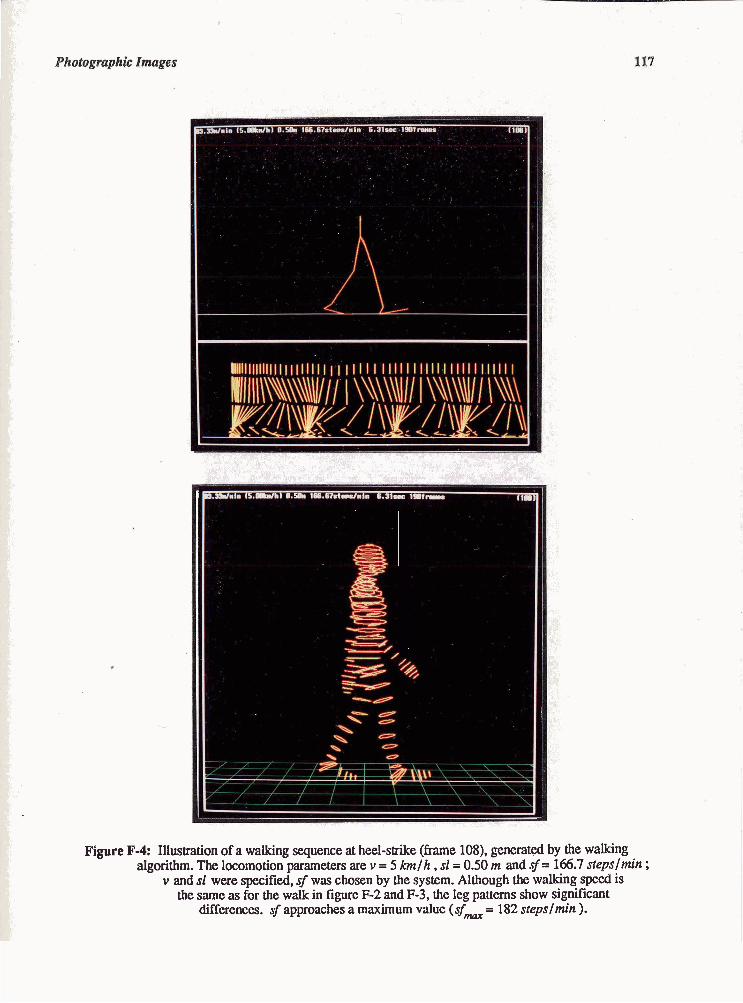
Figure F-4: Illustration of a walking sequence at heel-strike (frame 108), generated by the walking algorithm. The locomotion parameters are v = 5 kmlh , sl = 0.50 m and sf= 166.7 stepslmin ;
v and sl were specified, s f was chosen by the system. Although the walking speed is the same as for thc walk in figure F-2 and F-3, the leg patterns show significant
differences. sf approaches a maximum valuc (sf- = 182 stepslmin ).

Photographic Images
2 .. f,
Y"' .$
Figure F-5: Illustration of pelvic rotation in the transverse plane (a top view is assumed) for the walk shown in figure F-2. Top: heel-strike of left leg at frame 86. Middle:
mid-stance of left leg at frame 93. Bottom: heel-strike of right leg at frame 103.

Photographic Images
Figure F-6: Illustration of lateral displacement of the body for the walk shown in figure F-2. The body is shifted over the right leg (see arrow) at mid-stance for the right leg (frame 113).
- ncxt pagc - Top: at hml-strikc (framc 120), the body is ccntcrcd bclwccn Lhe Icgs.
Bottom: at mid-stance for the left leg (frame 130), the body is shifted over the left leg.


photographic Images I L
Figure P-7: Illustration of pelvic list in the coronal plane. Top: natural pelvic list at toe-off ( m e 106) for the walk shown in figure F-2. Bottom: accentuated
pelvic list at toe-off (frame 126) for the walk shown in figure F-3.

References
References
[Alexander 841
[Annsaong 851
[Badler 791
[Badler 801
[Badler 871
[Badler 881
[Beckett 681
[Burden 851
[Calvert $21
[Calvert 883
[Catmull 781
[Csuri 811
R.McN. Alexander. The Gaits of Bipedal and Quadrupedal Animals. The International Journal of Robotics Research 3(2):49-59,1984.
W.W. Annsmng, M. Green. The Dynamics of Articulated Rigid Bodies for Purposes of Animation. In Graphics Interjiie '85, Proceedings, pages 407-415. 1985.
N.I. Badler, S.W. Smoliar. Digital Representation of Human Movement. Computing Surveys 11(1):19-38, March, 1979.
N.I. Badler, J. O'Rourke, B. Kaufman. Special Problems in Human Movement Simulation. In ACM SIGGRAPH '80, Proceedings, pages 189-197. July, 1980.
N.I. Badler, K.H. Manoochehri, G. Walters. Articulated Figure Positioning by Multiple Constraints. IEEE Computer Graphics and Applications 7(6):28-38, June, 1987.
N.I. Badler. Human Figure Modeling and Animation. In Computer Graphics Symposium.'88. Hewbtt Packard, 1988.
R. Beckett, K. Chang. An Evaluation of the Kinematics of Gait by Minimum Energy. J. Biomechanics 1: 147- 159,1968.
R.L. Burden. Numerical Analysis. Prindle, Weber & Schmidt, 1985.
T.W. Calvert, J. Chapman, A. Palta. Aspects of the Kinematic Simulation of Human Movement. IEEE Computer Graphics and Applications 2(9):4 1-50, November, 1982.
T.W. Calvert. The Challenge of Human Figure Animation. In Graphics Interface '88, Proceedings, pages 203-210. 1988.
E. Catmull. A Hidden-Surface Algorithm with Anti-Aliasing. In SIGGRAPH '78, Proceedings, pages 6-11. July, 1978. .
C. Csuri. Goal-Directed Movement Simulation. In CMCCS '81 I ACCHO '81, pages 271-280. 198 1.

References
Pagg 771
[Drewery 861
[Forest 861
[Girard 851
[Gomez 851
[Greene 721
[Isaacs 871
A.I. Dagg. Running, Walking, Jumping. Wykeham Publications, London, 1977.
K. Drewery, J. Tsotsos. Goal-Directed Animation Using English Motion Commands. In Graphics Interface '86, Proceedings, pages 131-135. 1986.
L. Forest, N. Magnenat-Thalmann, D. Thalrnann. Keyframe based Subacmrs. In Graphics Interface '86, Proceedings, pages 213-216. 1986.
M. Girard, A.A. Maciejweski. Computational Modeling for the Computer Animation of Legged Figures. In ACM SZGGRAPH '85, Proceedings, pages 263-270. July, 1985.
JE. Gomez. TWMT: A 3-D Animation System. Computer & Graphics 9(3):291-298,1985.
P. H. Greene. Problems of Organization of Motor Systems. Progress in Theroretical Biology. Academic Press, New Yo*, 1972, pages 303-338.
P. Hanrahan, D. Sturman. Interactive Animation of Parametric Models. The Visual Computer 1:260-266,1985.
Alan C. Hindmarsh. LSODE and LSODI, Two New Initial Value Ordinary Differential Equation Solvers. ACM-SIGNUM Newsletter l5(4): 10- 11,1980.
V.T. Inman, WJ. Ralston, F. Todd. Human Walking. Williams & Wilkins, Baltimore, 198 1.
P.M. Isaacs, MI. Cohen. Controlling Dynamic Simulation with Kinematic Constraints, Behavior Functions and
Inverse Dynamics. Computer Graphics 21(4):215-224, July, 1987.
J.U. Korein, N.I. Badler. Techniques for Generating Goal-Directed Motion for Articulated Structures. IEEE Computer Graphics and Applications 2(9):91-81, November, 1982.
T. Lozano-Perez, M.A. Wesley. An Algorithm for Planning Collision-Free Paths among Polyhedral Obstacles. Communications of the ACM 22(10), October, 1979.
N. Magnenat-Thalmann, D. Thalmann. The Use of High-Level 3-D Graphical Types in the MIRA Animation System. IEEE Computer Graphics and Applications 3(9):9-16, December, 1983.
N. Magnenat-Thalmann, D. Thalmann. An Indexed Bibliography on Computer Animation. IEEE Computer Graphics and Applications 5(7):76-85, July, 1985.
References
WcGeer 881 B.T. McGeer. Passive Dynamic Walking. January, 1988. submitted for publication.
WMahon 841 T.A. McMahon. Mechanics of Locomotion. The International Journal of Robotics Research 3(2):4-28,1984.
Weirovitch 701 L. Meirovitch. Methods of Analytical Mechanics. McGraw-Hill, New York, 1970.
W l e r 753 D.I. Miller. Computer simulation of Human Motion. Techniques For The Analysis of Human Movement. Lepus Books, London, 1975, pages 69-105, Chapter 3.
Winsky 751 M. Minsky. A Framework for Representing Knowledge. The Psychology of Computer Vision. McGraw-Hill, New York, 1975.
Miura 841 H. Miura, I. Shimoyarna. Dynamic Walk of a Biped. The International Journal of Robotics Research 3(2):60-74,1984.
Nuybridge 701 E. Muybndge. Human & Animal Locomotion. Dover Publications, New York, 1970.
Wylopoulos 831 J. Mylopoulos, H. Levesque. An Overview of Knowledge Representation. On Computational Modelling: Perspectives from AI. Databases, and Programming
Languages. Springer-Verlag, New York, 1983.
Patla 851 AX. Patla, T. W. Calvert, R. B. Stein. Model of a Pattern Generator for Locomotion in Mammals.
, American Journal of Physiology 17(4):R484-R494,1985. Section R: Regulatory, Integrative and Comparative Physiology.
[pearson 761 K. Pearson. The Control of Walking. Scientific American 235(6):72-86,1976.
[Raibert 84a] M.H. Raibert. Hopping in Legged Systems - Modeling and Simulation for the 2D Case. IEEE Transactions Syst. Man Cybern. 14(3):451-463,1984.
[Raibert 84b] M.H. Raibert, H.B. Brown, Jr., M.Chepponis. Experiments in Balance with a 3D One-Legged Hopping Machine. The International Journal of Robotics Research 3(2):75-92,1984.
[Raibert 86a] M.H. Raibert. Legged Robots that Balance. MIT Press, Cambridge Massachusetts, 1986.

References
[Raibert 86bl
[Reynolds 821
[Ridsdale 861
[Ridsdale 871
[Sturrnan 86al
[S turrnan 86bl
[Sutherland 841
[vanBaerle 861
[Vaughan 82aI
[Vaughan 82bl
Wells 671
Wilhelms 851
Wilhelms 861
winter 793
[Zeltzer 82al
M.H. Raibert. Legged Robots. Communications of the ACM 29(6):499-514,1986.
C.W. Reynolds. Computer Animation with Scripts and Actors. In SIGGRAPH '82, Proceedings, pages 289-296. July, 1982.
G. Ridsdale, S. Hewitt, T.W. Calvert. The Interactive Specification of Human Animmation. In Graphics Interface '86, Proceedings, pages 121-130. 1986.
G J. Ridsdale. The Director's Apprentice: Animating Figures in a Constraint Environment. PhD thesis, Simon Fraser Unversity, 1987.
D. Sturman. Interactive Keyframe Animation of 3-D Articulated Models. In Graphics Interface '86, Tutorial on Computer Animation. 1986.
D. Sturman. A Discussion on the Development of Motion Control Systems. In Graphics Interface '86, Tutorial on Computer Animation. 1986.
I.E. Sutherland, M.K. Ullner. Footprints in the Asphalt. The International Journal of Robotics Research 3(2):29-36,1984.
S. van Baerle. Character Animation: Combining Computer Graphics with Traditional Animation. In Graphics Interface '86, Tutorial on Computer Animation. 1986.
C.L. Vaughan, J.G. Hay, J.G. Andrews. Closed h p Problems in Biomechanics. Part I - A Classification System. J. Biomechanics 15(3): 197-200,1982.
C.L. Vaughan, J.G. Hay, J.G. Andrews. Closed Loop Problems in Biomechanics. Part II - A Optimization Approach. J. Biomechanics 15(3):201-210,1982.
D.A. Wells. Theory and Problems of Lagrangian Dynamics. McGraw-Hill, New York, 1967.
J. Wilhelms. Using Dynamic Analysis to Animate Articulated Bodies such as Humans and Robots. In Graphics InterJace '85, Proceedings, pages 97-104. 1985.
J. Wilhelms. Virya- A Motion Control Editor for Kinematic and Dynamic Aniamtion. In Graphics Interface '86, Proceedings, pages 141-146. 1986.
D.A. Winter. Biomechanics of Human Movement. John Wiley & Sons, 1979.
D. Zelaer. Representation of Complex Animated Figures. In Graphics InterJaGe '82, Proceedings, pages 205-211. 1982.

References
[Zeltzer 82bl
[Zeltzer 851
[Zugck 841
D. Zeltzer. Motor Conml Techniques for Figure Animation. IEEE Computer Graphics and Applications 2(9):53-59,1982.
D. Zelber. Knowledge-Based Animation. In ACM SIGGRAPHISIGART, Workshop on Motion, pages 187-192. 1983.
D. Zeltzer. Towards an Integrated View of 3-D Computer Character Animation. In Graphics Interface '85, Proceedings, pages 105-1 15. 1985.
J. Zugck. Numerische Behandlung Linear-impliziter Differentialgleichungen mit Hilfe von
Extrapolationsmethoden. Master's thesis, University of Heidelberg, 1984.
Recommended


