Growing out of Poverty under Risk:

Evidence from Rural Ethiopia

Chris Elbers, Jan Willem Gunning and Lei Pan1

March 2, 2009

1At the time of this research all three authors were at the Department of Economics, VU University,Amsterdam and the Tinbergen Institute. Lei Pan is now at the Department of Economics, WageningenUniversity.

Abstract

The effect of risk on economic growth is a key issue in development but there is virtually no

evidence on it and little clarity on what determines the effect. In this paper we use panel

data for rural households in Ethiopia to estimate a structural model of household investment

decisions under risk. The sample households are heterogeneous in terms of initial capital

(livestock) and total factor productivity. The paper makes three contributions. First, we find

that risk substantially reduces growth in aggregate: for a household with median productivity

the capital stock converges (in expectation) to a mean which is only about one third lower

than what it would be in the absence of risk. This enormous impact largely reflects the ex

ante effect of risk. Secondly, the effect of risk on savings depends, not only quantitatively but

qualitatively on how productive households are. Thirdly, the welfare cost of risk is enormous:

the median household would be willing to pay two thirds of its initial wealth for actuarially

fair insurance.

JEL Codes: D10, D91, C51, O12

1 Introduction

What, if anything, keeps rural households in developing countries from growing out of poverty

on their own? In many cases, notably in areas with poor soils or inadequate rainfall, the answer

is simply that there are no profitable investment opportunities. In such areas poverty will persist

or people will escape from it through migration. Alternatively, profitable opportunities do exist

but households cannot exploit them: they are stuck in a poverty trap, typically because they

cannot overcome indivisibilities in investment through borrowing (Galor and Zeira, 1993). So

far, it has proved very difficult to find convincing empirical evidence of povety traps (e.g., Jalan

and Ravallion, 2005). A possible reason is the absence of risk in the multiple equilibria models

in the theory of poverty gaps. Clearly, if a sufficient amount of risk is introduced those models

behave very differently: a positive shock may enable a household to escape temporarily from

the trap and conversely a negative shock may push a rich household into a period of poverty. A

third type of answer is that poverty persists precisely because households face risk: exposure to

uninsured risk reduces the level of savings and biases its allocation in favor of low-return, low-

risk activities. There is much anecdotal evidence (particularly in the anthropological literature)

suggesting that rural households in Africa indeed adopt responses to risk which, while effective

as risk-coping strategies, have a high price in terms of foregone growth (Collier and Gunning,

1999). If this is true then policies which reduce risk exposure or that offer insurance would be

effective, not just in helping households to smooth consumption (the traditional rationale) but

also in promoting growth. Resolving which of these three explanations is correct is of crucial

importance but there is as yet very little empirical evidence (Lybbert et al., 2004, for Ethiopia

and Elbers et al., 2007, for Zimbabwe are among the few exceptions).

It is far from self-evident that the effect of risk on growth should be negative. In the

theoretical literature the effect of risk (in the sense of a mean preserving spread) on savings

1

has usually been studied in the standard additive model, typically under the assumption that

only labor income is risky. In that case the effect of risk on savings is positive, provided the

utility function exhibits prudence (e.g. Leland, 1968). Since most authors assume constant

relative risk aversion (which implies prudence, i.e. u′′′ > 0) a positive effect of risk on savings

(precautionary savings) is a standard result in this literature. The best-known model of risk

and savings for developing countries (Deaton, 1991) introduces a capital market imperfection

in the form of a borrowing constraint but in this model the effect of risk on savings can only

be positive.

Hahn (1970) showed that risk could reduce savings if it affects assets rather than labor

income. The sign of the effect therefore depends not only on preferences but also on the nature

of risk, notably on whether or not the agent has access to a safe asset (Gunning, 2008). Asset

risk is plausible in developing countries where households typically use assets such as livestock

or food stores which are affected by various risks (e.g. theft, illnesses, drought). The effect of

risk may therefore well be negative in such countries. In this paper we allow for both types

of risk, labor income risk and asset risk. Hence the sign of the effect of risk on savings is not

implied by our model; we rather leave it as an empirical matter, to be settled by the estimation

results.

We address these issues for one of the poorest countries in the world, Ethiopia. We use panel

data to estimate a structural model of savings and consumption decisions under risk. In this

model agents face risk but have no access to credit or insurance: using livestock for consumption

smoothing is the only way they can cope with risk. Livestock is also used as a productive asset.

Zimmerman and Carter (2003), Carter and Barrett (2006) and Carter et al. (2007) have argued

that in such a situation households will prefer asset smoothing over consumption smoothing:

rather than use assets to maintain consumption in the wake of a negative shock, consumption

will be adjusted so that future production possibilities are maintained. See also Fafchamps et

2

al. (1998). The literature on asset smoothing typically needs particular assumptions to produce

such an effect, for example by introducing a subsistence constraint. In this paper we are agnostic

on this issue: households choose their consumption and asset changes optimally and in principle

this can produce either asset or consumption smoothing. As it happens we find no evidence

of asset smoothing. Which account is more realistic is of considerable importance. Ethiopia

has instituted a large rural safety net program, covering some 800,000 households (Gilligan

and Hoddinott, 2007). In the asset smoothing world such downside protection should allow

households to grow rapidly. Conversely, under consumption smoothing the partial insurance

offered by the safety net will have a very limited effect: at higher asset levels risk can still have

a negative effect on growth.

The structure of the paper is as follows. We present the model, a stochastic version of the

Ramsey model, in section 2 and discuss the Ethiopia dataset in section 3. Section 4 discusses

how the model is estimated by simulation and presents the estimation results. In section 5 the

estimated model is used in simulation experiments. In particular we investigate how households

would behave in the absence of risk (or, equivalently, under actuarially fair insurance) and

compare this with the outcomes under risk. This comparison is used to estimate the effect

of risk on investment and on welfare. The willingness to pay for actuarially fair insurance is

calculated for various types of households as the compensating variation. We find that risk

has a very strong negative effect on accumulation. This is entirely the result of the ex ante

effect, the change in investment behaviour induced by exposure to risk: the ex post effect is

small and positive. We also find that household heterogeneity matters: for the least productive

households the two effects are both positive, for the most productive households they are both

negative. The effect of risk on savings therefore depends crucially on the agent’s productivity.

This is a novel result: the literature has focused on preferences and on the nature of risk, but

not on household productivity. Section 6 concludes.

3

2 The Model

We assume that there is a single good, used for consumption, as a store of value and also as a

productive asset. Agents maximise expected utility over an infinite horizon. Each household

solves for the optimal investment function ϕ(·):

maxϕ(·)

E0

∞∑t=0

βtu(ct) (1)

subject to

wt = syt af(kt) + sk

t (1− δ)kt

wt = ct + kt+1

kt+1 = ϕ(wt)

for t = 0, 1, 2, .. and w0 given

where w denotes wealth on hand, c consumption, k the capital stock corrected for land and

labour endowments (see Section 4), a total factor productivity, u the instantaneous utility

function, f the production function, β a discount factor, δ the depreciation rate, and t time.1

We assume strict concavity of u and f and 0 < β < 1. The investment decision is taken when

the shock realizations (syt , s

kt ) are known so that wt is given.

The household faces two types of risk: capital income risk (shocks sy) and asset risk (shocks

sk). We assume rational expectations: the household knows the distributions of these shocks.

The shocks are independently distributed across households and time and are lognormal with1See Stokey and Lucas (1989) for a detailed discussion of recursive optimisation models.

Total factor productivity is time invariant from the household’s point of view. In fact it changes, e.g. withhousehold size or land holdings. Such changes are modelled as part of the shocks to which the household isexposed.

4

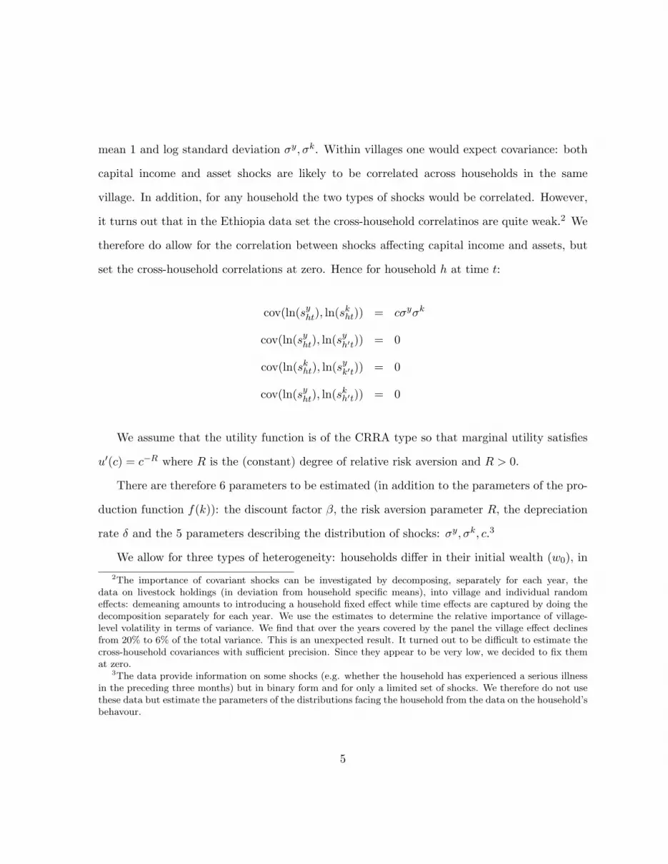
mean 1 and log standard deviation σy, σk. Within villages one would expect covariance: both

capital income and asset shocks are likely to be correlated across households in the same

village. In addition, for any household the two types of shocks would be correlated. However,

it turns out that in the Ethiopia data set the cross-household correlatinos are quite weak.2 We

therefore do allow for the correlation between shocks affecting capital income and assets, but

set the cross-household correlations at zero. Hence for household h at time t:

cov(ln(syht), ln(sk

ht)) = cσyσk

cov(ln(syht), ln(sy

h′t)) = 0

cov(ln(skht), ln(sy

k′t)) = 0

cov(ln(syht), ln(sk

h′t)) = 0

We assume that the utility function is of the CRRA type so that marginal utility satisfies

u′(c) = c−R where R is the (constant) degree of relative risk aversion and R > 0.

There are therefore 6 parameters to be estimated (in addition to the parameters of the pro-

duction function f(k)): the discount factor β, the risk aversion parameter R, the depreciation

rate δ and the 5 parameters describing the distribution of shocks: σy, σk, c.3

We allow for three types of heterogeneity: households differ in their initial wealth (w0), in2The importance of covariant shocks can be investigated by decomposing, separately for each year, the

data on livestock holdings (in deviation from household specific means), into village and individual randomeffects: demeaning amounts to introducing a household fixed effect while time effects are captured by doing thedecomposition separately for each year. We use the estimates to determine the relative importance of village-level volatility in terms of variance. We find that over the years covered by the panel the village effect declinesfrom 20% to 6% of the total variance. This is an unexpected result. It turned out to be difficult to estimate thecross-household covariances with sufficient precision. Since they appear to be very low, we decided to fix themat zero.

3The data provide information on some shocks (e.g. whether the household has experienced a serious illnessin the preceding three months) but in binary form and for only a limited set of shocks. We therefore do not usethese data but estimate the parameters of the distributions facing the household from the data on the household’sbehavour.

5

the shocks they experience and in productivity (a). In the absence of risk (syht = sk

ht = 1 for

all h and t) and if productivity is constant (aht = ah) then the model is simply the Ramsey

model and growth (in the sense of transitional dynamics) will exhibit conditional convergence:

the capital stock of household h will converge to the steady state value k∗h which satisfies

β[ahf′(k∗h) + (1 − δ)] = 1 (where f ′ denotes the marginal productivity of capital (livestock)

in agricultural production) and therefore depends on the household’s productivity ah. In our

sample most households’ initial asset holdings are far below this steady state value so that

there is substantial scope for growth: in the absence of risk households will increase their

capital stock by saving, approaching k∗h in the limit.

The central question in this paper is how risk affects this accumulation path. We measure

the effect of risk on accumulation as the difference between the expected value of the capital

stock at time T (E0khT ) when the household faces risk and the riskfree steady state value k∗h.4

The theoretical literature has focused on the question how preferences (risk aversion) determine

the sign of the effect of risk on savings. As is well known, under CRRA the effect is positive

if part of wealth is exogenous with respect to k and risk affects only this component (which

is usually called labor income).5 Labor income risk therefore induces an increase in saving:

precautionary saving. Conversely, if risk affects all wealth on hand (rather than only the part

that does not depend on k) then the effect has the sign of R−1 where R is the degree of relative

risk aversion (Hahn, 1970). Our specification differs from these familiar special cases: there

is exogenous labor income in the model but it represents only a minor component of wealth

w and we do not impose that risk affects the two components of wealth (income af(kht) and

assets (1 − δ)kht) equally. This implies that, even controlling for R, the sign of the effect of

risk on savings is not known a priori. Indeed we find that the effect, while positive for some4In simulation experiments we use a 90-year period: T = 90.5This is because CRRA implies u′′′ > 0 hence prudence; see Leland, 1968 and Kimball, 1990.

6

households, is negative for other households with the same preferences.6

Four implications of the stochastic Ramsey specification (1) should be noted. First, there is

a single asset. This rules out diversification as a risk coping strategy. In fact in the Ethiopian

sample livestock dominates asset ownership so this is not overly restrictive. Secondly, there are

no indivisibilities: k is a continuous variable. This is restrictive: while the Ethiopian small-

holders hold much of their livestock as goats, sheep and chickens (which can be reasonably

be modelled as continuous) they also invest in oxen. This is a major investment which intro-

duces indivisibilities.7 Thirdly, the model does not allow for credit, insurance or informal risk

pooling. There is in fact very little credit and insurance in rural Ethiopia despite the finding

in footnote 8 that shocks are overwhelmingly idiosyncratic. See e.g. Rosenzweig and Stark

(1989); Grimard (1997); Dercon and Krishnan (2003); De Weerdt (2002); Hoddinott et al.,

(2005). Pan (2008) has used the data on transfers in the Ethiopian dataset to investigate local

risk pooling. She finds that transfers between households do not reflect risk pooling: observed

shocks experienced by the households have no significant effects on the transfers they receive

or send. She also finds that transfers received from government agencies (often donor sup-

ported) and NGOs mitigate covariant shocks somewhat but that these transfers are so poorly

targeted that this form of insurance is trivial: only a very small part of the covariant shocks is

compensated by such transfers.8 She therefore models the transfers received by households as6Gunning (2008, Table 3) shows in a two-period model that the effect is positive for capital income risk if

R ≥ 1 (and ambiguous otherwise) and negative for asset risk if R ≤ 1 (and ambiguous otherwise). Our estimatefor R is in fact extremely close to 1 (log utility). Hence (at least in the 2-period model) asset risk has a negativeeffect but capital income risk a positive one. Which effect dominates is an empirical question.

7Rosenzweig and Wolpin (1993) model allow for indivisibilities, modelling bullocks holdings as a discretevariable. Usually parameter estimates of such models are highly correlated and parameters are therefore difficultto estimate precisely (Elbers et al., 2008). Rosenzweig and Wolpin overcome this problem by fixing one of theparameters. Vigh (2008) used the same Ethiopian data and extended the present model by distinguishingbetween ‘goats’, a continuous variable, and ‘oxen’, a discrete variable. She demonstrates the feasibility of thisextension but since it imposes considerable computational burdens we here use the simpler specification.

8Dercon and Krishnan (2003) find that aid received by the village has a significant effect on a household’sconsumption. While they interpret this as risk sharing it probably reflects income redistribution (Pan, 2008a):transfers received from NGOs or government agencies (‘aid’) are very weakly correlated with shocks but richer

7

independent of shocks.9 Finally, we assume that shocks are independent across time. Allowing

for autocorrelation would impose substantial computational burdens since the policy function

would then no longer be recursive.

3 Data

We use the panel data of the Ethiopia Rural Household Survey (ERHS), collected by the Eco-

nomics Department of Addis Ababa University, the Center for the Study of African Economies

at the University of Oxford and the International Food Policy Research Institute (IFPRI).

The EHRS is one of the few long running panel data sets available at the household level in

Africa. In 1989, some 450 households in six locations were surveyed for a famine study. In the

beginning of 1994 this sample was extended to 1,477 households in 15 villages. The sample was

stratified so as to ensure an adequate coverage of the main farming systems and of households

which might be very vulnerable, female headed and landless households. The households of

this larger sample were re-interviewed in the second half of 1994 and again in 1995, 1997, 1999

and 2004. (Later rounds are not yet publicly available.) Since the 1989 survey used a very

different questionnaire from the later rounds and also covered a smaller sample we only use the

1994 (second round), 1995, 1997, 1999 and 2004 data. We therefore have five observations per

household.

The survey provides detailed information on household income, assets and consumption.

Household income consists of income from crops and livestock, wage income and transfers.

Transfers include support from the government and NGOs (notably food aid), gifts and remit-

recipients of such aid transfer part of it to poorer households.9Pan (2008a) regressed transfers on various household characteristics. We include transfers as predicted by

these regressions in the constant of the function f(k); deviations from the regression line are included in theshock sk.

8

tances. They account for about 15% of total income (Pan, 2008, Table 2.2).

Land is allocated by Peasant Associations10 and cannot be sold. It can therefore not be used

as a consumption smoothing asset. Table 1 gives descriptive statistics for aggregate income,

Table 1: Descriptive Statistics: Income, Livestock and ConsumptionYear Obs. Mean sd Min Median Max

Income 1994 1,477 2,478 5,519 0 (43)a 1,332 143,9731995 1,468 2,433 3,923 0 (13) 1,448 63,2341997 1,415 4,119 22,361 0 (21) 1,986 748,4341999 1,385 3,239 4,093 0 (8) 2,282 55,9002004 1,340 2,954 5,062 0 (1) 2,018 142,549

Livestock 1994 1,477 1,799 3,021 0 889 70,0171995 1,477 1,557 2,620 0 788 62,4841997 1,415 2,302 3,210 0 1,346 36,7621999 1,385 1,841 2,118 0 1,191 24,8862004 1,325 2,276 3,279 0 1,285 53,575

Consumption 1994 1,472 4,481 4,162 85 3,238 43,8891995 1,422 3,855 3,546 146 2,859 36,9381997 1,409 5,569 4,295 154 4,389 40,2171999 1,382 5,387 4,355 85 4,011 38,3672004 1,299 5,600 5,216 143 4,051 48,154

Note.—The values are in Birr in 1994 prices. 1 Birr ≈ 0.1 USD.a The number of the observations with zero income.

livestock ownership and consumption by year. Households with zero income were excluded

from the analysis.11

Income, livestock holdings and consumption all increased in the period 1994-97. However,

Table 1 shows a fall in income and livestock holdings between and 2004; this reflects the food

crises of 1999-2000 and 2002-2003.10In Ethiopia, a peasant association is not a farmers’ self-help group as the name might suggest, but the lowest

tier of civil administration, covering one or more villages.11These probably reflects missing values for the prices used in constructing household income.

9

The table shows a large discrepancy between income and consumption levels. In the surveys

households were asked to recall their income in the previous year or since the previous round

of the survey. This long recall period may have led to substantial underreporting of income.

Consumption data are based on recall over the preceding month. The data were then multi-

plied by 12 to get an annual amount.The income and the consumption data are only weakly

correlated: the correlation coefficient is around 0.1.

The ERHS also collected information on household characteristics such as household size,

composition and educational attainment. Some information on shocks was also collected in the

survey, for example whether the rain came on time in the previous farming season, whether

there was enough rainfall, whether diseases affected people, crops or livestock, and births and

deaths of livestock. However, these shocks data are in binary form and are therefore not suitable

for estimating the distributions of sy and sk.

4 Estimating the Model

The estimation proceeds in three steps. In the first step we estimate the income function

af(k).12 In the second step we derive the policy function which solves the stochastic Ramsey

model. The policy function gives the optimal value of kht as a function of wealth on hand wht

for a given set of parameters (β,R, δ, σy, σk, c). 13 An important and convenient implication

of our specification is that the policy function takes a recursive form kht = ϕ(wht, aht−1): this

function is the same for all h and t. The third step involves using Simulated Pseudo Maximum12In principle the income function should be estimated simultaneously with the rest of the model. However,

since the function involves a large number of parameters this would impose an excessive computational burden.We estimate the income function directly without regard for the first order conditions for factor use since thelarge shocks imply that these conditions will be violated. The estimation procedure is discussed in detail in Pan(2008, ch. 2, appendix A).

13Note that the optimal consumption level follows immediately from cht = wht − f(wht).

10

Likelihood Estimation: using the policy function we calculate the likelihood by simulation.14

to estimate the 6 parameters (β,R, δ, σy, σk, c). We now consider these three steps in turn.

The Income Function

We use the income function estimated by Pan (2008, ch. 2), based on Cockburn (2002): income

y (including transfers) is a CES function of livestock (k), labor (lab) and land (lan):15

yt = a(α1k−ρt−1 + α2lab

−ρt−1 + α3lan

−ρt−1)

− τρ ×

exp(∑

i

ηixit−1+∑

p

λpwspt+∑

q

χqosqt+∑

j

φjvj +∑

o

ψodo + et), (2)

labt−1 = labmt−1 + κ1labft−1 + κ2lab

ct−1, (3)

eht = gvt + bh + nht, (4)

cov(eht, eht′) = cgtt′σ2g + σ2

b + cntt′σ2n = σ2

tt′ . (5)

In equations (2) and (3) we have suppressed the household index h for readability. Returns to

scale are captured by τ and the scope for substitution between production factors by ρ. The

labour force lab is defined in equation (3) in terms of adult male equivalents on the basis of

the number of males, females and children in the household. The specification implies that

labour use is fully determined by labour availability.16 Income depends not only on the three

production factors but also on a series of shocks (weather shocks ws and other shocks os), village

(vj) and time (do) effects in (2). Here xit denotes household characteristics (e.g. whether the

14See e.g. Gourieroux and Montfort (1996), Section 3.2.15To simplify the notation we suppress the subscript h in the first two equations (where it applies to all

variables except the year dummies).16This is clearly restrictive since there is evidence that households vary labour use in response to shocks (e.g.

Kochar, 1999 and. Jacoby and Skoufias, 1997, for the ICRISAT villages in India and Giles, 2006, for China.The Ethiopia surveys did not collect data on labour use. To the extent households varied labour use in responseto shocks our estimate of the shock sy captures the shock after such adjustment.

11

household is female headed or whether it grows a particular crop). The parameters αi, ρ, τ ,

κi, ηi, φj , ψo, λp and χq must be estimated.

The error term includes unobserved village specific shocks (gvt), household effects (bh) and

the unobserved idiosyncratic shock nht. These shocks are assumed to be distributed normally:

gvt ∼ N(0, σ2g), bh ∼ N(0, σ2

b) and nht ∼ N(0, σ2n). cgtt′ is the correlation of the village specific

shocks at year t and at year t′ and cntt′ is the correlation of the unobserved idiosyncratic shocks

at year t and at year t′.

The income function is estimated with Generalized Least Squares. The results are shown

in Table 2.

The estimated value of ρ implies a substitution elasticity of 3.5. We find decreasing re-

turns to scale (τ < 1). The estimates for the labour force conversion factors (0.784 for adult

females) and 0.454 for children) are quite reasonable. In order to reduce the dimensions of the

intertemporal optimization problem equation (2) can be written in ‘intensive’ form, scaling by

the combined land and labour factors Aht = (α2lab−ρht−1 + α3lan

−ρht−1)

−1/ρ:

yht = aht−1(α1k−ρht−1 + 1)−

τρ exp(eht +

∑p

λpwspht +∑

q

χqosqht +∑

o

ψodot), (6)

where

yht =yht

Aht(7)

kht =kht

Aht(8)

aht−1 =a exp(

∑i ηixiht−1 +

∑j φjvjh)

A1−τht

. (9)

12

Table 2: Estimation Results: Income Function (Generalised Least Squares)Dependent variable: IncomeIndependent variables Coef. t-statistic

returnd to scale (τ) 0.628∗∗∗ 24.83substitution (ρ) −0.716∗∗∗ −9.60livestock (α1) 0.281∗∗∗ 11.77labor (α2) 0.280∗∗∗ 8.07land (α3) 0.439∗∗∗ 14.62female adults (κ1) 0.784∗∗∗ 5.92children (κ2) 0.454∗∗∗ 5.40landless 0.373∗∗∗ 6.43land quality 0.121∗∗∗ 4.71coffee grown 0.251∗∗∗ 5.41qat grown 0.224∗∗∗ 4.57false banana grown −0.124∗∗ −2.45eucalyptus grown 0.114∗∗∗ 4.06female headed −0.130∗∗∗ −4.50head age −0.003∗∗∗ −3.73head education 0.025∗∗∗ 7.45village dummies

Haresaw −0.341∗∗ −2.03Geblen −0.857∗∗∗ −5.03Dinki −0.523∗∗∗ −3.12Yetmen 0.103 0.61Shumsha 0.040 0.24Sirbana 0.402∗∗ 2.42Adele 0.115 0.67Korod 0.020 0.12Turfe 0.466∗∗∗ 2.77Imdibir 0.012 0.07Azedeboa −0.174 −0.97Addado 0.470∗∗∗ 2.61Garagodo −0.445∗∗ −2.54Doma −0.598∗∗∗ −3.52

year dummies1995 −0.011 −0.111997 0.227∗∗ 2.381999 0.443∗∗∗ 4.552004 0.276∗∗∗ 2.88

constant 6.921∗∗∗ 48.92observed shocks not reportedobservations 6, 749R-squared 0.39

Note—The parameter α3 is calculated as 1− α1 − α2.∗ Significant at the 10% level.∗∗ Significant at the 5% level.∗∗∗ Significant at the 1% level.

13

The model can now be written as:

maxϕh(·)

E0

∞∑t=0

βtu(cht) (10)

subject to

wht = syhtaht−1(α1k

−ρht−1 + 1)−

τρ + sk

ht(1− δ)kht−1 (11)

wht = cht + kht (12)

kht = ϕh(wht) (13)

for t = 0, 1, .. and wh0 given,

where wht and cht are again scaled by Aht:17

wht = wht/Aht,

cht = cht/Aht.

The policy function

In the second step we derive the policy function kht = ϕh(wht) = ϕ(wht, aht−1) for the model (1).

This function gives the optimal level of investment kht as a function of the household’s wealth

on hand wht and productivity aht−1 for a given set of parameters (β,R, δ, σy, σk, c). Suppressing17Scaling consumption will affect the expression that is to be maximized. However, with CRRA utility

functions the policy function, and consequently the accumulation process, is not affected by scaling consumptionif the scaling factor is constant or if changes in the scaling factor are treated as completely unanticipated shocksand farmers expect the current value of the scaling factor to persist forever. The reason is that marginal utilityenters the Euler equation (equation 14) as a factor on both sides, so that a constant scaling factor drops out ofthe equation—from marginal utility, not from the production function.

14

the household index h optimal investment satisfies the Euler equation:

u′(wt − kt) = βEu

′(wt+1 − kt+1)

∂wt+1

∂kt

. (14)

We use the iterative procedure described in Elbers (2009) to derive the policy function.

This procedure requires maximizations with respect to k of expressions of the form

u(w − k) + βEu(w(k, sy, sk)− ϕ(w(k′, sy, sk))), (15)

where w(k, sy, sk) follows from equation (11) and ϕ(·) is an approximation of the policy function.

The solution defines a new approximation of the policy function and the procedure is iterated

until convergence. We calculate the expectations in (15) as the average over (the same) 100

draws from the joint distribution of (sy, sk), defined by parameters (σy, σk, c).18 Note the policy

functions are household-specific and depend on the parameters to be estimated.

Estimation

There are six parameters which need to be estimated in this model: β, γ, δ, σy, σk, and c.

These parameters are estimated using Simulated Pseudo Maximum Likelihood. There are 5

observations for each household and we calculate the likelihood of the observed transitions of

kh as:

LL = L(kh95|kh94)L(kh97|kh95)L(kh99|kh97)L(kh04|kh99).

Consider L(kh97|kh95) as an example. Given the observed value kh95 and randomly generated

shocks (syh96, s

kh96, s

yh97, s

kh97) the values wh97 and kh97 can be simulated using the policy function

for the current set of parameter values. This is done for 200 shock values and the mean µh97 and18This is also the procedure used in Pan (2008, Chapter 4).

15

variance σ2h97 of the simulated values of log(kh97) are then calculated. Given these moments

the pseudo likelihood of log(kh97) is calculated, using the normal probability density function.

Proceeding in the same way for each of the four intervals the loglikelihood LL follows. We use

simulated annealing19 to maximize the likelihood with respect to the parameters.

Parameter estimates

Table 3 shows the estimates of the parameters. The estimate of δ is equal to 0.002 indicating

that the depreciation rate on livestock is quite low. Our estimate of γ is extremely close

to zero, suggesting a log utility function.20 The estimate of β implies a discount rate of

approximately 9%. The shock parameters σy and σk indicate that the Ethiopian households

face huge shocks. For example, the estimate of σk implies that a positive shock of one standard

deviation, increases livestock holding 51%. The correlation of the (log) income and asset shocks

is found to be surprisingly low. One would expect strong positive correlation between the two

types of shocks (as was found for Zimbabwan farmers by Elbers et al. 2007), but this is not

what the Ethiopia data indicate.

5 Results

We first consider the aggregate effect of risk on accumulation. For this we calculate the expected

value of livestock at the end of a 90-year period (Ek90) for a household with the median value

of productivity (a = 0.9). The expectation is calculated as the mean over 100,000 simulation

paths. For a household with this level of productivity the capital stock would converge to a

value of 4.67 if there were no risk. Under risk we find an expected value Ek90 = 2.97. Hence19See e.g. Ross (2006), Section 10.4.20Elbers et al. (2007) also find evidence of log utility.

16

Table 3: Estimation Results for the Ramsey ModelParameter Estimate Standard Error

δ 0.002 0.002γ 0.000 0.004β 0.913 0.007σy 0.776 0.072σk 0.412 0.035c 0.045 0.005

Number of households 919−2× log(LL) 8566.89

Note.—Households with less than four observations or with missing values for live-stock are excluded. Standard errors are based on bootstrapping using 48 replications.

the effect of risk is to reduce the capital stock in expectation by 36%.21 We can decompose

this into the ex ante and ex post effects by simulating the model under the assumption that

the agent correctly perceives the distribution of shocks but never actually experiences a shock

(sy = sk = 1). In this case we find Ek90 = 2.73. Hence the ex ante effect reduces the capital

stock in expectation by 42%22. It follows that the ex post effect is positive, but relatively small,

increasing the capital stock by 5%.

We now consider how the effect of risk may differ between households, depending on their

productivity (a). Table 4 shows the simulation results for five values of a, including the median

case (a = 0.9) which we have already considered. The results are striking: the results for these

five productivity levels are very different, not only quantitatively, but also qualitatively. In

the first two cases both effects are positive; in the third case the ex ante effect is negative but

the ex post effect is positive (and larger in absolute magnitude); in the fourth case the ex ante

effect is negative and the ex post effect is again positive but now smaller in absolute magnitude;

and in the last case both effects are negative. This has important implications. For example,21As it happens, this is similar to the 46% reduction reported by Elbers et al. (2007) Zimbabwe (for a shorter

similation period: t = 50). However, in that case the ex ante and ex post effects are both negative.222.73/4.67-1=-0.415.

17

it has been suggested that the introduction of insurance (or, more generally, measures to help

rural households in risk coping) will have the effect of inducing more saving (e.g. Dercon, 2005,

Elbers et al., 2007, ILO, 2008). In effect such measures would give households the incentive to

grow out of poverty through increased saving. If our results generalize this is true for households

above a certain level of productivity, but not if the intervention is targeted at the very poorest

households, those with very low productivity.

In the sample we find households of all five types. Table 5 shows the distribution of the

sample over the four types, the boundary values for productivity and the signs of the ex ante

and the ex post effects.23 Note that type 1 accounts for only 0.4% of the sample and type 2

for 3.6%. Of the Ethiopian households 59% belong to type 3 and 37% to type 4. Hence for the

vast majority of the households in our sample the effect of risk on accumulation is negative and

dominated by the ex ante effect.24 This is important since in much of the empirical literature

(e.g. Ravallion, 1988, Dercon and Krishnan 2000, Dercon 2004) it is implicitly assumed that

the effect of actual shocks adequately measures the effect of risk. Clearly, this only picks up the

ex post effect which, at least for the vast majority of the households in the Ethiopia sample,

accounts for a only a very small part of the total effect.

Table 4: Effect of Risk on Expected Livestock Holdings after 90 years (Ek90)no risk: risk: risk:

ex ante ex ante and % changeeffect only ex post effects from risk free case

a k∗ Ek90 Ek90 total ex ante ex post0.274 0.102 0.267 0.375 267.6 162.0 105.60.332 0.244 0.382 0.520 113.4 56.9 56.50.544 0.993 0.870 1.116 12.4 -12.4 24.80.900 4.670 2.730 2.970 -36.4 -41.5 5.11.255 11.788 6.645 6.054 -48.6 -43.6 -5.0

23Here the larger effect (in absolute value) is denoted ++ or −−.24This conforms the findings of the Zimbabwe study, Elbers et al. (2007).

18

Table 5: Productivity and the Effect of Risk on Savingsproductivity (a) effect of risk

on savingsmin max % of sample ex ante ex post0 0.449 5 + ++0.449 0.586 8 − ++0.586 1.069 50 −− +1.069 ∞ 37 −− −

Figure 1 shows the evolution of the expected capital stock over time, for the four chosen

values of a. The Figure shows that the four types do not only differ in the signs and magnitude

of the long-run effects of risk. There are also remarkable differences in transitional dynamics.

For the very poor households (types 1 and 2) there is very rapid accumulation in the early

years and little change in k or Ek after 20 years. More productive households continue to

accumulate significantly (in expectation) even after 50 years. We also find that in some cases

the accumulation paths cross. For type 2, the ex ante effect is initially positive, later negative.

Similarly, for type 4 the ex post effect is first positive and then negative. These results indicate

that the effect of risk on growth (in the sense of transitional dynamics) is more subtle than

previously appreciated. The sign and magnitude depends not just on preferences (notably the

degree of risk aversion) and on the type of risk agents face (Gunning, 2008) but also on the

household’s productivity and on the length of the period considered.

It is instructive to compare the policy functions for type 1 (very poor) and type 3 (median)

households. Figure 2 shows the policy functions with and without risk for a = 0.274 and

a = 0.900 respectively. For a = 0.274 the two policy functions cross at a wealth level of

approximately w = 0.5. For lower values of wealth (and those are the relevant values for such

a household) the no risk policy function is lower than the one when shocks are expected. This

confirms that the ex ante effect is positive for this household. Now consider the ex post effect.

19

In the Figure this amounts to a mean preserving spread of w: the policy function is not affected

but shocks change the value of w. Note that for a = 0.274 the policy functions are strictly

convex before they cross and are thereafter almost linear. This explains that for type 1 the ex

post effect is large and positive.25 For a = 0.900 the policy functions are strictly convex but

virtually linear in the relevant range. This is why we find a positive but relatively small effect.

We now consider welfare effects. Measuring welfare as expected discounted utility over

the simulation period (E0∑90

t=1 βtu(ct)) Table 6 reports welfare for 16 types of households

(for each of the 4 productivity levels considered before we report welfare for 4 values for the

initial capital stock k0).26 Columns (4) and (5) show the welfare cost of risk, in the sense of

compensating variation (CV), calculated as the transfer received at t = 1 under risk which

would increase the level of expected utility to the level of welfare in the risk free case. We show

the CV, separately for the ex ante effect alone and the ex post effect.27 These costs can be

compared to the (pre-transfer) level of wealth on hand w1 in the risk free case, shown in the last

column. Clearly, the welfare costs are enormous. For example, for a household with median

productivity (a = 0.900) the two compensating variations amount to 99% of initial wealth

on hand (k0 = 0), 66% (k0 = 0.921), 57% (k0 = 1.803) and 51% (k0 = 4.005), respectively,

depending on the initial value of livestock.28 Such a household would therefore be willing to

pay more than half of its wealth on hand (possibly much more than that) for actuarially fair

insurance. In terms of income these percentages would be considerably higher. This suggests

that these poor households would be willing to pay a substantial part of their total income as

a premium if they would have access to insurance. Note that the percentage is highest for the25By Jensen’s inequality strict convexity implies that an increase in risk (in the sense of a mean preserving

value of w) induces (in expectation) more accumulation. Hence the effect of risk on investment is positive.26The results are very similar for the case c2 = c3 = 0.3.27Recall from Table 4 that the ex ante effect often dominates the effect of risk on savings. This is not the case

for its effect on welfare: the CV for the ex post effect is invaraiably far larger than the CV for the ex ante effect.28In the first case: (0.050+0.845) as a percentage of 0.900.

20

poorest households.

Table 6: Welfare costs of riskwelfare levels welfare changes:

no risk ex ante both compensating variations initial wealtheffect only effects ex ante ex post w1

(1) (2) (3) (4) (5) (6)a k = 0 (min)

0.274 -15.165 -15.288 -16.794 0.029 0.343 0.2740.332 -12.837 -12.93 -14.43 0.026 0.406 0.3320.544 -6.653 -6.673 -8.222 0.009 0.665 0.5440.9 0.089 0.061 -1.661 0.018 1.174 0.91.255 4.912 4.862 2.892 0.042 1.827 1.255

k = 0.921 (30th percentile)0.274 -12.39 -12.42 -13.664 0.013 0.608 1.2560.332 -10.359 -10.375 -11.626 0.008 0.682 1.3270.544 -4.78 -4.781 -6.113 0.002 0.979 1.5880.9 1.547 1.513 -0.056 0.031 1.604 2.0261.255 6.172 6.112 4.254 0.067 2.408 2.462

k = 1.803 (60th percentile)0.274 -10.593 -10.621 -11.98 0.016 0.897 2.1740.332 -8.72 -8.735 -10.079 0.009 0.973 2.2530.544 -3.485 -3.496 -4.875 0.009 1.291 2.5430.9 2.578 2.531 0.936 0.05 1.998 3.031.255 7.064 6.994 5.117 0.091 2.913 3.515

k = 4.005 (90th percentile)0.274 -7.384 -7.439 -9.163 0.047 1.784 4.4470.332 -5.751 -5.79 -7.455 0.036 1.854 4.5430.544 -1.06 -1.103 -2.701 0.049 2.187 4.890.9 4.552 4.479 2.731 0.106 3.053 5.4751.255 8.79 8.7 6.703 0.154 4.191 6.057

21

6 Conclusion

Can poor households grow out of poverty by their own actions? Put differently, what keeps

them from doing so? The literature has given two types of answers. One strand argues in effect

that most poor households have no access to attractive investment opportunities: their only

hope to escape from poverty is therefore to migrate to a location where their labour commands

a higher return. Another strand argues that profitable investment opportunities do exist but

that poor people cannot exploit them, typically because a combination of indivisibilities in

investment and capital market imperfections (as in Galor and Zeira, 1993) traps them in a

low-level equilibrium or because a combination of high risk exposure and poor risk pooling

institutions makes saving unattractive. This last possibility has often been raised as a constraint

on investment in Africa: exposure to uninsured risk is then seen as a disincentive to investment

(e.g. Collier and Gunning, 1999, Dercon, 2005). While in much of the literature on risk and

savings (particularly for developed countries) there is a presumption of a positive effect (risk

inducing precautionary savings) the effect may well be negative, notably if risk affects asset

returns rather than labour income.

Investigating this possibility of a negative effect of risk on growth empirically faces serious

problems of specification, estimation techniques and data availability. Randomised trials (where

households in the treatment group would be given insurance) could be used to estimate the

effect of risk on investment and would have the advantage of not requiring a model. This

approach is being implemented, notably to assess the impact of health insurance in Africa.

It would seem impractical, however, to extend this approach from testing a specific form of

insurance to a comprehensive insurance package. The answer to the question how risk affects

growth can then at best be answered for a subset of the risks faced by households. Alternatively,

regression analysis can be used if shocks can be measured. However, unless quite long time

22

series are available this will give biased estimates, identifying the ex post effect of risk but

underestimating the ex ante effect. Also, the method fails if at least some of the risk is the

same for all households. In this paper we have used the methodology of Elbers et al. (2007)

where the effect is identified by estimating a model of investment decisions under risk in its

structural form. Identification is then obtained from the Euler equation. This method does

not require observations on shocks but it does require panel data. Regarding specification,

the best known model for developing countries of household saving under risk (Deaton, 1991)

implies that risk, far from being a constraint on accumulation, actually stimulates saving if

the underlying utility function is of the CRRA type. The stochastic Ramsey model we have

used does not imply the sign of the effect of risk on growth. Whether the effect is positive or

negative is therefore an empirical matter.

The paper makes three contributions. First, we find that in one of the poorest areas of

Africa, rural Ethiopia, uninsured risk has a very substantial effect on capital accumulation.

For the median household in our sample the expected long-run capital stock is in our base case

36% lower than in the absence of risk. We have decomposed this into an ex ante effect (-41.5%)

and an ex post effect (+5.1%).29 It is possible for these households to grow out of poverty for

our estimates imply strong transitional dynamics: in the absence of risk the consumption level

of the median household would grow on average by 3.5% per year over the first 20 years and

would continue to grow rapidly thereafter. Risk reduces the average growth rate in the first 20

year (to 1.9%) and there is very little growth thereafter. In that sense risk presents a formidable

impediment to poverty reduction.30

Secondly, we have shown that the effect of risk on growth does not only depend on prefer-29Note that in the case of Ethiopia methods which focus on the ex post effect would get both the sign and the

size of the total effect wrong.30Elbers et al. (2007) found similar results for Zimbabwe. The present paper suggests that this was not due to

some Zimbabwe-specific aspect of the data. In addition we feel more confident about the present results becausein this paper we approximate the solution of the Euler equation much more accurately.

23

ences and the nature of the risk faced, the two determinants on which the literature focuses.

Households with the same preferences can respond very differently to the same risks if they

differ in productivity. Such heterogeneity leads to results which differ not only quantitatively,

but also qualitatively. For the least productive households the ex ante and ex post effects

are both positive, for the most productive households they are both negative. This is a novel

result: to the best of our knowledge the literature has not recognised that the effect of risk

on savings behaviour depends crucially on the agent’s productivity. Our finding suggests that

the effect that the introduction of insurance would have on growth31 depends critically on the

characteristics of the targeted group.

Thirdly, the Ethiopian households are exposed to enormous risk. We established this de-

scriptively (considering the distribution of livestock holdings), econometrically (by estimating

the parameters of the distributions of shocks facing the households) and, perhaps most re-

vealingly, in terms of welfare. We calculated the compensating variations a household would

require to accept the actual situation rather than a risk-free counterfactual. At the median

level of productivity we found that households would require a compensation equivalent to at

least 65% of their initial wealth on hand. Put differently, these households would be willing to

use a substantial part of their resources to acquire actuarially fair insurance. Disturbingly, risk

affects the welfare of the poorest households most (as measured by the compensating variation

relative to initial wealth).31The effect of insurance on welfare (as opposed to growth) is of course unambiguously positive.

24

25

Figure 1: Simulation results

Type 1: Productivity ah=0.274

Type 2: Productivity ah=0.544

Type 3: Productivity ah=0.9

Type 4: Productivity ah=1.255

26

Figure 2: The ex ante effect of risk:

Policy functions with and without risk

References

Abramowitz, Milton and Irene A. Stegun (eds., 1972), Handbook of Mathematical Functions, New

York, Dover, 9th printing.

Ayalew, D. (2003), ‘Risk-Sharing Networks among Households in Rural Ethiopia’, Working Paper

186, Centre for the Study of African Economies, University of Oxford.

Browning, M. and A. Lusardi, 1996, Household Saving: Micro Theories and Micro Facts, Journal

of Economic Literature, vol. 34, pp. 1797-1855.

Carter, Michael and Christopher B. Barrett (2006), ‘The Economics of Poverty Traps and Persis-

tent Poverty: an Asset-Based Approach, Journal of Development Studies, vol. pp.

Carter, Michael R., Peter D. Little, Tewodaj Mogues and Workneh Negatu (2007), ‘Poverty Traps

and Natural Disasters in Ethiopia and Honduras, World Development, vol. 35, pp. 835-856.

Cockburn, J. (2002), ‘Income Contributions of Child Work in Rural Ethiopia’, Working Paper No.

2002-12, Center for the Study of African Economies, University of Oxford.

Collier, Paul and Jan Willem Gunning (1999), ‘Explaining African Economic Performance’, Journal

of Economic Literature, vol. 36, pp. 64-111.

Deaton, Angus (1991), ‘Saving and Liquidity Constraints’, Econometrica, vol. 59, pp. 1221-1248.

Dercon, Stefan (2004), ‘Growth and Shocks: Evidence from Rural Ethiopia’, Journal of Develop-

ment Economics, vol. 74, pp. 309-329.

Dercon, Stefan (2005), ‘Risk, Insurance and Poverty: a Review’, in: Stefan Dercon (ed.), Insurance

against Poverty, Oxford: Oxford University Press, pp. 9-37.

Dercon, Stefan and Pramila Krishnan (2000), ‘Vulnerability, Seasonality and Poverty in Ethiopia’,

Journal of Development Studies, vol. pp. 25-53.

Dercon, Stefan and Pramila Krishnan (2003), ‘Food Aid and Informal Insurance’, Discussion Paper

No. 2003/09, World Institute for Development Economics Research, Helsinki, Finland.

27

Elbers (2009), ‘Solving the Discrete-Time Stochastic Ramsey Model’. Tinbergen Institute discus-

sion paper TI 09-018/2. Tinbergen Institute, Amsterdam.¡

Elbers, Chris, Jan Willem Gunning and Bill Kinsey (2007), ‘Growth and Risk: Methodology and

Micro Evidence’, World Bank Economic Review, vol. 21, pp. 1-20.

Elbers, Chris, Jan Willem Gunning and Lei Pan (2008), ‘Insurance and Rural Welfare: What Can

Panel Data Tell Us?’, Applied Economics, January.

Epstein, Larry G. and Stanley E. Zin (1991), ‘Substitution, Risk Aversion, and the Temporal

Behavior of Consumption and Asset Returns: an Empirical Analysis’, Journal of Political

Economy, vol. 99, pp. 263-286.

Fafchamps, M., Udry, C., Czukas, K. (1998), ‘Drought and saving in West Africa: are livestock a

buffer stock?’, Journal of Development Economics, vol. 55, pp. 273-305.

Galor, O. and J. Zeira (1993), ‘Income Distribution and Macroeconomics’, Review of Economic

Studies, vol. 60, pp. 35-52.

Giles, J. (2006), ‘Is Life More Risky in the Open? Household Risk-Coping and the Opening of

China’s Labor Markets’, Journal of Development Economics, vol. 81, pp. 25-60.

Gilligan, Daniel O. and John Hoddinott (2007), ‘Is There Persistence in the Impact of Emergency

Food Aid? Evidence on Consumption, Food Security, and Assets in Rural Ethiopia, American

Journal of Agricultural Economics, vol. pp.

Gourieroux, Christian and Alain Monfort (1996), Simulation-based Econometric Methods, New

York: Oxford University Press.

Grimard, F. (1997), ‘Household Consumption Smoothing through Ethnic Ties: Evidence from

Cote d’Ivoire’, Journal of Development Economics, vol. 53, pp. 391-422.

Gunning, Jan Willem (2008), ‘Risk and Savings’, Tinbergen Institute Discussion Paper 2008-071/2.

Hahn, Frank (1970), ‘Savings and Uncertainty’, Review of Economic Studies, vol. 37, pp. 21-24.

Hoddinott, John, Stefan Dercon and Pramila Krishnan, ‘Networks and Informal Mutual Support in

28

15 Ethiopian Villages’, Working Paper, Centre for the Study of African Economies, University

of Oxford.

ILO (2008), Research Strategy 2008-2012, Microinsurance Innovation Facility, International Labour

Office, Geneva.

Jacoby, H. G. and E. Skoufias (1997), ‘Risk, Financial Markets, and Human Capital in a Developing

Country’, Review of Economic Studies, vol. 64, pp. 311-335.

Jalan, Jyotsna and Martin Ravallion (2005), ‘Household Income Dynamics in Rural China’, in

Stefan Dercon (ed.), Insurance against Poverty, Oxford: Oxford University Press.

Kochar, A. (1999), ‘Smoothing Consumption by Smoothing Income: Hours-of-Work Responses to

Idiosyncratic Agricultural Shocks in Rural India’, Review of Economics and Statistics, vol. 81,

pp. 50-61.

Kimball, M.S., 1990, ‘Precautionary Saving in the Small and in the Large’, Econometrica, vol. 58,

pp. 53-73.

Leland, H.E. (1968), ‘Saving and Uncertainty: the Precautionary Demand for Saving’, Quarterly

Journal of Economics, vol. 82, 465-473.

Lybbert, T.J., C.B. Barrett, S. Desta and D.L. Coppock (2004), ‘Stochastic wealth dynamics and

risk management among a poor population’, Economic Journal, vol. 114, pp. 750-777.

Pan, Lei (2008), Poverty, Risk and Insurance: Evidence from Ethiopia and Yemen, PhD thesis,

VU University Amsterdam and Tinbergen Institute.

Pan, Lei (2008a), ‘Risk Pooling through Transfers in Rural Ethiopia’, Economic Development and

Cultural Change, forthcoming.

Ravallion, Martin (1988), ‘Expected Poverty under Risk-Induced Welfare Variability’, Economic

Journal, vol. 98, pp. 1171-1182.

Rosenzweig, Mark R. and Oded Stark (1989), ‘Consumption Smoothing, Migration, and Marriage:

Evidence from Rural India’, Journal of Political Economy, vol. 97, pp. 905-926.

29

Rosenzweig, Mark R. and Kenneth Wolpin (1993), ‘Credit Market Constraints, Consumption

Smoothing, and the Accumulation of Durable Production Assets in Low-Income Countries:

Investment in Bullocks in India’, Journal of Political Economy, vol. 101, pp. 223-244.

Ross, S.M. (2006), Simulation, 4th edition, Burlington, San Diego and London: Elsevier Academic

Press.

Stokey, Nancy L. and Robert E. Lucas Jr. (1989), Recursive Methods in Economic Dynamics,

Cambridge, Mass.: Harvard University Press.

Vigh, Melinda (2008), Risk Coping in Rural Ethiopia: the Liquidity and Productivity of Livestock,

MPhil thesis, Tinbergen Institute.

Weerdt, Joachim de (2002), ‘Risk-sharing and Endogenous Network Formation,

WIDER Discussion Paper 2002/57, Helsinki.

Zimmerman, Frederick J. and Michael R. Carter (2003), ‘Asset Smoothing, Consumption Smooth-

ing and the Reproduction of Inequality under Risk and Subsistence Constraints, Journal of

Development Economics, vol. 71, pp.

30