Download pdf - Hierarchical constraint logic programming

J. LOGIC PROGRAMMING 1993:16:277-318 277

HIERARCHICAL CONSTRAINT LOGIC PROGRAMMING

MOLLY WILSON AND ALAN BORNING

D Constraint logic programming (CLP) is a general scheme for extending logic programming to include constraints. It is parametrized by z%, the domain of the constraints. However, CLP(9) languages, as well as most other constraint systems, only allow the programmer to specify constraints that must hold. In many applications, such as interactive graphics, planning, document formatting, and decision support, one needs to express preferences as well as strict requirements. If we wish to make full use of the constraint paradigm, we need ways to represent these defaults and preferences declaratively, as constraints, rather than encoding them in the procedural parts of the language. We describe a scheme for extending CLP(9) to include both required and preferential constraints. An arbitrary number of strengths of preference are allowed. We present a theory of such constraint hierarchies, and an extension, hierarchical constraint logic programming (HCLP), of the CLP scheme to include constraint hierarchies. We give an operational, model theoretic, and hxed-point semantics for the HCLP scheme. Finally, we describe two interpreters we have written for instances of the HCLP scheme, give example programs, and discuss related work. a

1. INTRODUCTION

Constraint logic programming (CLP) is an extension of logic programming that significantly increases the expressiveness of such languages. Jaffar and Lassez ‘[34] describe a general scheme for such extensions, which is parametrized by 9, the domain of the constraints. The language that arises from a fixed vocabulary of constraints over 59 can be denoted by CLP(g). In place of unification (which can be viewed as testing the satisfiability of equations over the Herbrand universe),

Address correspondence to AIan Boming, Department of Computer Science and Engineering, FR-3.5, University of Washington, Seattle, Washington 98195. Email: [email protected].

Received December 1991; accepted March 1993.

THE JOURNAL OF LOGIC PROGRAMMING

OElsevier Science Publishing Co., Inc., 1993

655 Avenue of the Americas, New York, NY 10010 0743-1066/93/$6.00

278 M. WILSON AND A. BORNING

constraints are accumulated and tested for satisfiability over 9, using techniques appropriate to the domain. Several such languages have now been implemented, including CLP@) [35, 361, Prolog III [ill, CHIP [14, 771, CAL [61], CLP CC*) 1791, and Echidna [69].

The formal semantics of such languages differ primarily in the choice of underlying domain and constraints, as was shown formally in [34]. It was also shown that for every CLP language, numerous desirable properties of the declarative and operational semantics hold-properties that had been considered characteristic of logic programming. In particular, CLP languages have coincident logical, fixed- point, and operational semantics.

Constraints have also been embedded in a number of other languages and systems, and have proven useful for a wide variety of applications, including user interface toolkits, geometric layout, physical simulations, user interface design, document formatting, algorithm animation, and design and analysis of mechanical devices and electrical circuits. (See [20] and [39] for surveys.)

Many applications of constraints either need, or would benefit from, support for default and preferential constraints, as well as required ones. Such constraints are sometimes called soft constraints; the required ones are hard constraints. A set consisting of both hard and soft constraints is a constraint hierarchy.

Our own work on constraint hierarchies has been application oriented and driven primarily by pragmatic concerns. ThingLab [3], for example, was a constraint-based laboratory that allowed a user to construct simulations of such things as electrical circuits, mechanical linkages, demonstrations of geometric theorems, and graphical calculators using interactive direct-manipulation techniques. All the explicit constraints in ThingLab, for example, that a line in a geometric figure be horizontal or that a resistor in an electrical simulation obey Ohm’s law, were required. The user’s edit requests were implicitly treated as strong preferences rather than requirements, so that if the edit conflicted with a required constraint, the user’s constraint would be overridden. (One of the HCLP examples in Section 4.1 is taken from the original ThingLab, and illustrates this behavior.) In addition, there were implicit weak or very weak constraints that parts of an object keep their old values as the object was being manipulated by the user, unless it was necessary for them to change to satisfy the user’s edit or the explicit required constraints. Some of these implicit weak constraints needed to be stronger than others to achieve intuitive behavior. For example, suppose that we have a simple graphical calculator that includes a constraint A + B = C. Now suppose the user edits the value of A. As we might expect, ThingLab would resatisfy the + constraint by changing C, rather than by changing B. Also, if a preferential constraint cannot be satisfied, we may still wish to satisfy it as well as possible, rather than simply ignoring it if it cannot be satisfied completely (again see Section 4.1).

ThingLab lacked a separate, declarative theory of hard and soft constraints that specified what to do in cases such as those just described. Instead, these choices were embedded in the procedural code of the constraint satisfier. (This was also true of all the other early applications-oriented constraint systems, such as Sketch- pad [74], Magritte [29], and Juno [49].) This situation became increasingly trouble- some when we tried to improve on ThingLab’s constraint satisfier, because there was no declarative specification that we could use to decide whether a particular optimization would lead to a correct answer. In response, a version of the

HIERARCHICAL CONSTRAINT LOGIC PROGRAMMING 279

constraint hierarchy theory described in this paper was developed, and was used in subsequent versions of ThingLab.

This theory has served well to describe declaratively the behavior we desired in interactive graphics applications. For example, we can use weak constraints to specify that objects in a picture remain stationary during editing unless there is some constraint or user edit that forces them to move. Error metrics associated with the constraints allow us to minimize the error in satisfying constraints if they cannot be satisfied completely.

It also has turned out that the constraint hierarchy theory has been useful for domains other than interactive graphics. For example, in a scheduling application, some constraints might be requirements, whereas others would be only preferences (such as not scheduling a meeting too early in the morning). As before, some of the preferences may be stronger than others. For example, it might be strongly preferred that the meeting last an hour, but only weakly preferred that it begin at 9:00 a.m. In a graph layout application, it might be required that two nodes be at least a minimum distance apart, and preferred that they be aligned vertically. In a planning system for manufacturing, there may be required constraints on the order in which operations are done on a part, and preferences about which machines are to be used to perform the operations.

ThingLab, as well as the other applications, used a constraint package built on top of an existing language. However, there are many benefits to having constraint hierarchies completely integrated with a programming language. For example, in an integrated language we will be assured that the constraints are considered and there is no need to call the constraint satisfier explicitly. (In a package, the programmer might simply ignore the constraints.) An integrated system allows more opportunities for optimizing the implementation. Finally, in the case of logic programming, there is an elegant theory available (the CLP scheme).

We are thus led to extend the CLP scheme to include both hard and soft constraints and to implement instances of this language scheme. The hierarchical constraint logic programming scheme HCLP(g,%?) is parametrized both by the domain ~3 of the constraints and by the comparator %Y’, which is used to select among alternate ways of satisfying the soft constraints. In the remainder of the paper, we first present a theory of constraint hierarchies. We then describe the HCLP(53,ZY) scheme, give examples of its use for various domains and comparators, and describe a formal semantics for this family of languages. We also describe two HCLP interpreters we have written. The first is a straightforward interpreter, written in CLP(.%?), for HCLP(~,_ZY’B’), where _Y”B’ is the locally-predicate- better comparator to be described in the next section. The second is a more flexible but complex interpreter, written in Common Lisp, for HCLP@?, * 1. In this version the comparator used can be selected by the programmer from a number of possibilities.

Our original publication of the HCLP work is in reference [7]. The present paper significantly extends and modifies that work: It includes a revised theory of constraint hierarchies, a formal semantics that properly accounts for the preferential levels of constraints and that includes both a model theory and a fixed-point semantics, a discussion of the new HCLP(W, * ) interpreter, and an extended set of HCLP examples. A more complete discussion appears in Wilson’s Ph.D. dissertation [801. Other related work is discussed in Section 10.


2. CONSTRAINT HIERARCHIES

A constraint is a relation over some domain 9. The domain 9 determines the constraint predicate symbols II, of the language, which must include = . A constraint is thus an expression of the form p(t ,,. . ., t,>, where p is an n-ary symbol in II, and each ti is a term. A labeled constraint is a constraint labeled with a strength, written Zc, where 1 is a strength and c is a constraint. The strengths are totally ordered.

A constraint hierarchy is a finite set of labeled constraints. Given a constraint hierarchy H, Ha is a vector of the required constraints in H, in some arbitrary order, with their labels removed. H, is a vector of the constraints in H at the strongest nonrequired level, and so forth through the weakest constraints H,,, where n is the number of nonrequired levels in the hierarchy. We also define Hk = 0 for k > n.

A valuation for a set of constraints is a function that maps the free variables in the constraints to elements in the domain 9 over which the constraints are defined. A solution to a constraint hierarchy is a set of valuations for the free variables in the hierarchy. We require any valuation in the solution set to satisfy at least the required constraints. In addition, the solution set contains those valuations that satisfy the nonrequired constraints at least as well as any other valuation that also satisfies the required constraints. In other words, there is no valuation satisfying the required constraints that is “better” than any valuation in the solution. There are a number of reasonable methods for comparing valuations to determine which is better. We call such methods comparators. In the following sections we give formal definitions for the solution to a constraint hierarchy and for various comparators.

2.1. Error Functions

To compare valuations, we will need some measure of how well a particular valuation satisfies a given constraint. The error function e(c0> is used to indicate how nearly constraint c is satisfied for a valuation 8. This function returns a nonnegative real number and must have the property that e(ce) = 0 if and only if co holds. (~0 denotes the result of applying the valuation 0 to c.) For any domain g, we can use the trivial error function that returns 0 if the constraint is satisfied and 1 if it is not. A comparator that uses this error function is a predicate comparator. For a domain that is a metric space, in place of the trivial error function, we can define an error function by using the domain’s metric. For example, the error for X = Y would be the distance between X and Y. Such a comparator is a metric comparator. Because the definition of a specific comparator depends on the error function used, metric comparators are domain dependent.

The error function E(C0) maps e over a vector of constraints C = [c,, . . . , c,]:

E(C0) = [e(c,8) ,..., e(c,0)].

An error sequence is a vector [EC H, O 1, E( H, O>, . . . , E( H, 6 )I. Finally, the error ui for the ith constraint can be weighted by a weight wi. Each

weight is a positive real number.


2.2. Combining Functions

Some of the comparators that we are interested in will first combine the errors at a given level in the hierarchy before comparing valuations. We now introduce the notion of a combining function, g, that is applied to real-valued vectors and that returns some value that can be compared using the associated relations < >g and

5 . For example, g may sum a vector of numbers or select the maximum of a vector of numbers. We require <g to be irreflexive, antisymmetric, and transitive. We require < >g to be reflexive and symmetric. (We use the notation < >s rather than = because, for some of the comparators, the relation is not transitive. The symbol < >g indicates that two valuations cannot be ordered using <g . For some comparators, this will be because they are equal; for others, because they are incomparable.)

The combining function G is a generalization of g that is applied to error sequences and that returns a sequence of values that can be compared using < >g and <g . Such a sequence is a combined error sequence. Let R =

[E(H,0),..., E(H, 0)J. Then

G(R) = [s(E(H,8)),...,g(E(H,e))]

A lexicographic ordering -c~ can be defined on combined error sequences ur, . . . , u, and w ,, . . . , w,, in the standard way:

Ul,..., u, <g WI,...,W,

if 3kE l... nsuchthatViEl*..k-1 ui< >,~Au~<~IQ.

Finally, we can define the solution set S to a constraint hierarchy H by using the comparator defined by the combining function g, its associated function G, and the lexicographic ordering defined by <g :

So = (0lVc EH,e(cB) = 0},

s= @%sOAVCTES,

S, is the set of solutions to the required constraints (ignoring the soft constraints). The desired set S is all valuations in SO for which no better valuations in S, exist, where better is determined using the lexicographic ordering defined by <g .

2.3. A Brief Example

Before we give definitions for various comparators, a brief example will help to solidify the notion of a solution to a constraint hierarchy.

Let us consider the following simple constraint hierarchy over the domain of the reals:

required x>o strong x< 10 weak x=4

The set S, consists of all valuations that map X to a positive real number. The solution set S consists of the single valuation that maps X to 4. Let us call this


valuation 8. Consider the valuation (+ that maps X to 5. Then e((X < 1010) is 0. e((X< lo)(+) is also 0. E([(X< lO>e]) is [O]. (Th ere is only one constraint at the strong level.) E([(X < lO>a]> is also [O]. e((X = 418) is 0. e((X = 410) is 1. E([(X = 4)8] is [O]. E([(X= 4)(+]) is [l]. The combined error sequence G(E([(X < lO>f3]), E([(X = 4>0])> evaluates to [[O], [O]]. (Again, there is only one constraint at each level in the hierarchy, so the combining function has no effect.) The combined error sequence G(E([(X < 10)~ I), E([(X = 4)a])) evaluates to [LO], [ill. Because [[O], [O]] < [[O], [l]], (+ is not in S. Moreover, there is no valuation in S, that is less than [[O],[O]] in the lexicographic order defined by any cg , where <g and < >s have the properties defined previously. So 8 is in S.

2.4. Comparators

We now define a number of comparators, each of which gives rise to a different way of defining the set of solutions to a constraint hierarchy. We can classify types of comparators (as opposed to defining a specific comparator) as either global, local, or regional. Because the error sequences for the constraints at levels H 1,. . . , H, are being compared using a lexicographic ordering, if a solution 8 is better than a solution u, there is some level k in the hierarchy such that for 1 I i <k, g(E(Hie)) < >g g(E(Hi(+))> and at level k, g(E(H, 0)) -c~ g(E( Hk cr >I.

For a local comparator, each constraint is considered individually. Solution 0 must do exactly as well as u for each constraint in levels 1 a.* k - 1, and at level k, 8 must do at least as well as u for all constraints, and strictly better for at least one. For a global comparator, the errors for all constraints at a given level are aggregated using g. For a regional comparator, each constraint at a given level is considered individually (as with a local comparator). However, unlike a local comparator, two solutions that are incomparable at strong levels may still be compared at weaker levels and one discarded, so that a regional comparator will, in general, discriminate more than a local one.

We now define a number of useful classes of comparators, by defining the combining function g and the relations < >g and -K~ for each. Each of these classes defines some number of actual comparators by specifying the error function and weights on constraints.

Weighted-sum-better, worst-case-better, and least-squares-better are global comparators in which the constraint errors at a given level are combined by taking the weighted sum, the weighted maximum, and weighted sum of the squares, respectively. Locally-better and regionally-better are local and regional comparators, respectively.

For weighted-sum-better, g(v) = C!.v,I 1 wiui, <g is defined as for the reals and < >g is equivalent to = for the reals.

For worst-case-better, g(v) = max{wiui( 1 I i I Ivl), cg is defined as for the reals and < >g is equivalent to = for the reals.

For least-squares-better, g(v) = CpJ 1 wi$, cg is defined as for the reals and < >g is equivalent to = for the reals.

For locally-better, g(v) = v and < >g and cg are defined as v <g u = Vi ui 5 ui A 3j such that 9 < uj, v< >,u=Viui=ui.


For regionally-better, g(v) = v and < >g and cg are defined as

v<,u~~ivi~ui~3jsuchthat~<uj,

v< >,u= +<,u) “(u<,v)).

Orthogonal to the choice of a global, local, or regional combining function, we can choose an appropriate error function for the constraints. Locally-predicate-better (LPB) is locally-better using the trivial error function that returns 0 if the constraint is satisfied and 1 if it is not. Locally-metric-better is locally-better using a domain metric in computing the constraint errors. Weighted-sum-predicate-better, weighted-sum-metric-better, and so forth, are all defined analogously.

2.5. A Simple Example of the Differences Among the Comparators

As a simple example to illustrate some of the differences among the comparators, consider a constraint-based spreadsheet or a graphical calculator such as described in [3]. Suppose there is a “sum” constraint relating real-valued variables A, B, and C. Previously, the values for these variables were A = 2, B = 3, and C = 5. The user has just edited C to be 7. The following constraint hierarchy expresses the desired semantics:

required C=A+B strong c=7 weak A=2 weak B=3

The required C = A + B constraint represents the sum constraint. The strong C = 7 constraint represents the user’s edit. (Making this constraint a strong preference rather than a requirement allows the system to refuse to accept the edit if it conflicts with some required constraint; if instead we wished to be notified of a failure in this case, we would make the edit also required.) The two constraints weak A = 2 and weak B = 3 express a desire that the rest of the system be changed as little as possible in accommodating the edit to C. Without them, A = l,OOO,OOO, B = -999,993, and C = 7 would be a perfectly valid result.

We now list the solutions for a number of the comparators, assuming that the domain of the problem is the reals.

Locally-predicate-better yields two solutions:

A=2, B=5, c = 7, and

A =4, B=3, c = 7.

In the first solution, the A = 2 constraint is satisfied but not B = 3; in the second, B = 3 is satisfied but not A = 2.

Locally-metric-better yields an infinite number of solutions:

A =x, B=7-x, C=7 forall x~[2***4].

None of the solutions in the set is better than any other in the set. For example, the solution A = 2.9, B = 4.1, C = 7 does not satisfy the constraint on A as well as A = 2, B = 5, C = 7, but does better for the constraint on B.


However, outlying solutions such as A = l,OOO,OOO, B = - 999,993, and C = 7 are ruled out.

Weighted-sum-predicate-better yields the same two solutions as locally- predicate-better if the weights on the two weak constraints are equal; otherwise it picks one solution or the other depending on which weight is larger. (More generally, weighted-sum-predicate-better with weights of 1 for each constraint counts the number of unsatisfied constraints in comparing solutions, a useful property.)

Weighted-sum-metric-better yields the same infinite set of solutions as locally- metric-better if the weights on the two weak constraints are equal; otherwise it picks either A = 2, B = 5, C = 7, or A = 4, B = 3, C = 7, respectively, depending on whether the weight on the constraint on A or on B is larger.

Least-squares-metric-better yields a single solution, which is A = 3, B = 4, C = 7 when the weights on the weak constraints are equal. (This is also the solution for worst-case-metric better with equal weights.)

For this example, the regional comparators yield the same solutions as their local counterparts.

2.6. Which Comparator to Use?

There has not yet been enough experience to make any conclusive statements about which comparators, embedded in an HCLP language, are most appropriate for which classes of problems. However, there is considerable work in related areas that sheds some light on the question. (The comparators are all derived from previous formalisms, rather than being ad hoc inventions.)

The global comparators weighted-sum-error-better, worst-case-error-better, and least-squares-error-better are all derived from (and are generalizations of> the standard statistical measures of deviation L,-norm, L,-nomz, and L,-norm, respectively. Locally-error-better is derived from the concept of a vector minimum (or pareto-optimal point or nondominated feasible solution) in multiobjective linear programming problems [45]. In operations research, the choice between an L,, L,, or L, approximation seems often to be made on the class of constraints (for example, are they linear or nonlinear?) and the consequent difficulty of solving the resulting problem. The set of vector-minimum solutions is appealing mathemati- cally-the only solutions that could reasonably be of interest belong to this set-but working with this set of solutions has not been particularly practical [45].

As discussed in the introduction, our own work on constraint hierarchies originated as a rational reconstruction of the behavior of ThingLab and other constraint-based systems. Our recent work on constraint-based systems for user interface toolkits (ThingLab II [44, 431 and Multi-Garnet [56]) has used the locally-predicate-better comparator. This choice has been based primarily on pragmatic rather than aesthetic or theoretical grounds: the existence of efficient incremental algorithms-DeltaBlue [20] and a derivative algorithm SkyBlue [55]-for finding LPB solutions. For user interface applications, we do have extensive experience in the practical use of LPB [57]. It also has been used by a considerable number of researchers at other institutions as well. LPB has generally


proved quite satisfactory. However, for precise layout least-squares-better will often yield more aesthetic results. (The graphical layout system TRIP [37], for example, uses least-squares-better.)

2.7. Existence of Solutions

If the set of solutions S, for the required constraints is nonempty, intuitively one might expect that the set of solutions S for the hierarchy would be nonempty as well. However, there are some pathological hierarchies for which this is not the case. Consider the hierarchy required N > 0, strong N = 0 for the domain of the real numbers, using a metric comparator. Then S, consists of all valuations mapping N to a positive number, but S is empty, because for any valuation {N e d) E S,, we can find another valuation, for example (N e d/2}, that better satisfies the soft constraint N = 0.

However, the following propositions do hold:

Proposition 1. Zf S, is nonempty and finite, and if the < >g relation associated with the chosen comparator is transitive, then S is nonempty.

PROOF. Suppose to the contrary that S is empty. Pick a valuation 0, from S,. Because 8, @S, there must be some 0, ES, such that better(o,, 8,, H). Similarly, because 8, e S, there is a & E S, such that better(e3, f3,, HI, and so forth for an infinite chain e,, 0,, . . . . Because better is transitive, it follows by induction that Vi, j > 0 [i > j + better(@, e,, HI]. The irreflexivity property of better requires that Vi > 0 7 better-(&, ei, HI. Thus all the 0, are distinct, and so there are an infinite number of them. However, by hypothesis S, is finite, a contradiction. q

Proposition 2. Zf S, is nonempty, and if a predicate comparator is used, then S is nonempty.

PROOF. Suppose to the contrary that S is empty. Using the same argument as before, we show that there must be an infinite number of distinct valuations 0, E S,. However, if the comparator is predicate, one valuation cannot be better than another if both valuations satisfy exactly the same subset of constraints in H. Therefore, each of the Bi must satisfy a different subset of the constraints in H. However, this is a contradiction, because H is finite. q

3. OPERATIONAL SEMANTICS OF HCLP

An HCLP rule (or clause) takes the form

p(t): - 41(t) ,...,q,(t),l,cl(t),...,l,c,(t),

where t is a list of terms, p(t), q&t), . . . , q,(t) are atoms and Ire,(t), . . . , I,c,(t) are labeled constraints. (In actuality, the atoms and constraints may include different lists of terms, but for simplicity we use t, which is a list of all terms contained in the predicates and constraints of the rule.) An HCLP program is a collection of rules. A goal or query is a multiset of atoms. Whereas in practice, a goal may also contain constraints, without loss of generality, we will view goals as consisting only of atoms. (Any goal consisting of constraints can be renamed as a new predicate, and


then this predicate can become the new goal.) Operationally, goals are executed as in CLP, temporarily ignoring the nonrequired constraints, except to accumulate them. After a goal has been successfully reduced, the answer may still not be unique. In this case, the accumulated hierarchy of nonrequired constraints is then solved, using a method appropriate for the domain and the comparator %?, thus further refining the valuations in the solution. Additional valuations may be produced by backtracking.

We present the notion of a derivation for a query Q to capture the operational behavior of an HCLP program. We assume in what follows that selected rules undergo a variable transformation to ensure that they do not clash with existing variables. For each step in the derivation, an atom from the goal list is matched against the head of a rule in the program P, that atom is removed from the list of goals, and the atoms on the right hand side of the rule are added to the new goal list. (A computation rule determines which atom will be selected next. A fair computation rule is one in which each atom that appears in the derivation is chosen at some step.) The constraints are added to the constraint hierarchy. In addition, required equality constraints are created between the arguments in the selected atom and the arguments in the head of the selected rule. These constraints are treated no differently than any other constraints and are merely accumulated and added to the hierarchy. If there is no solution to the required constraints in the hierarchy, then the derivation is said to have failed. If there is some element in the derivation sequence such that all of the goals in the goal list have been reduced, and if there is a solution to the resulting constraint hierarchy, then the derivation is said to have succeeded. The final constraint hierarchy is the hierarchy associated with this empty goal list. A solution to this final hierarchy is then a solution to the original query.

More formally, a derivation for a program P and a query Q with selection rule R is a (possibly infinite) sequence of tuples G,, G,, . . . . Each tuple Gi consists of a goal list and a constraint hierarchy. We define

G, = (Q, Ho = 0).

Note that H’,H’,... are the hierarchies for Go, G,, . . . , in contrast to Ho,H1,..., H,,, which are the sets of constraints in the hierarchy H at levels O,l,..., IZ, respectively.

Let Gi be a tuple of the form ({p,(x,), . . . ,p,(x,J, Hi), where S,(H’) f 0. If there is a rule

in P and if R selects the atom p,(xj) at step i, then

Gi+r = ({PI(X,),..., p,(x,)) - {Pjtxj)} ” (4*(t),...,4m(t)l~

Hi u {llc,(t) ,...,lkCk(f)] u {t=Xj}).

In the preceding equation, {p,(x,), . . . , p,(x,>) - (pi( are the remaining unre- duced goals from Gi, {q,(x,>, . . . , q,(x,)} are the new goals from the rule, H’ is the previous hierarchy, {l,c,(t), . . . , l,c,(t)} are the new constraints from the rule, and {t = xi} are the required constraints that result from equating each argument in t with its corresponding argument in xi. For this derivation to be successful, it must


be the case that &,(H’+ I) # 0. We emphasize that this derivation step is relative to the rule

Pj(t):-q,(t),...,q,(t),',c,(t) ,...,bk(t)P

i.e., if some other rule with head pj were used at this step, then another derivation would result.

A derivation is successful if there is some tuple Gr = (0, Hf) in the derivation sequence and if the hierarchy Hf has a solution. Hf is known as the final constraint hierarchy. A valuation s is a computed solution for the query Q iff Q has a successful derivation with final constraint hierarchy Hf and s is a solution for Hf A derivation is finite& failed if there is no rule in P whose head has the same predicate symbol as the atom selected at a given step or if the set of required constraints at some step in the derivation has no solutions or if the final constraint hierarchy has no solutions. (See Section 2.7 for cases where there are no solutions to constraint hierarchies even when there is a solution for the required constraints.) A query is finitely failed if every derivation for that query is finitely failed. Let FF, denote the finite failure set with respect to a program P:

FF, = ( QlQ is finitely failed} .

If a goal succeeds, an interpreter will return an answer. An answer consists of a set of constraints (without strength annotations) on the variables in the initial goal. Additional answers may be produced by backtracking. Each answer represents one or more valuations in the solution to the constraint hierarchy. For example, the answer X = 2 represents the single valuation that maps X to 2, whereas the answer Y > 5 represents an infinite set of valuations, with each member of the set mapping Y onto a different number greater than 5. We make this distinction between answers and valuations because, on the one hand, we obviously prefer that an algorithm return Y > 5 rather than an infinite number of valuations. On the other hand, it is easier to define the comparators in terms of valuations rather than answers.

4. HCLP EXAMPLES

In this section we present a number of examples of HCLP programs. The programs here are all simple, but are illustrative of the use of constraint hierarchies for a variety of application areas. In the discussions, we try to emphasize the significance of the different possible comparators and how one or another might be most appropriate for a given application. All of the sample programs here are for the domain of the real numbers. (However, implementations of HCLP languages for other domains are of course possible as well, and would be useful for other applications. For example, the HCLP language CHAL [62, 631 includes support for the domain of the Booleans, as well as for polynomial equations over algebraic numbers. See also the discussion of this language in Section 10 on related work.)

Regarding the comparator to be used, if it is significant, we will refer to the program as, e.g., an HCLP(9’,_999’) one, but if any of various comparators might be appropriate, we will refer to the code simply as an HCLP(9’) program.

An HCLP program can include a list of symbolic names for the strength labels, which in an implementation are then mapped to the nonnegative integers. If the


label on a constraint is omitted, the label defaults to required; weights default to 1. For brevity, we assume that for all the program examples in this paper, the following strengths have been defined: required, strong, medium, and weak.

4.1. Interactive Graphics Examples

As discussed in the introduction, our original motivation for the definition of constraint hierarchies was to support interactive graphics in a more declarative manner. The following example is illustrative of a wide class of such programs. We have a horizontal line displayed on the screen, and we are moving one endpoint with the mouse (Figure 1). There is a required constraint that the line be horizontal, a medium constraint that one endpoint of the line follow the mouse, and a weak constraint that the endpoints of the line remain fixed. This weak constraint gives stability to the line as it is moved, so that, for example, it does not suddenly triple in length as we move the endpoint by some small distance.

The HCLP(9) rule that follows expresses the desired update behavior:

move-horiz-end2(line-segment(OldXl,OldY1,OldX2,OldY2),

line_segment(NewXl,NewYl,NewY2),

delta(DX,DY)):-

required OldYl=OldY2, required NewYl=NewY2,

medium OldX2+DX=NewX2, medium OldY2+DY=NewY2,

weak OldXl=NewXl, weak OldYl=NewYl,

weak OldX2=NewX2, weak OldY2=NewY2.

It takes as arguments terms representing the old and new states of the horizontal line, and a third term that is the x-y distance by which one endpoint should be moved. Any or all of the terms may contain variables. However, in typical use in an interactive graphics application, the old state of the line and the displacement would be ground, whereas the new state of the line would be a variable whose value would be computed as a result of satisfying the constraints.

Suppose now we anchor the other end of the horizontal line, so that this other end becomes difficult to move (Figure 2). We will use a strong rather than a required constraint, so that the anchor could be moved if needed by using an even stronger mouse constraint:

move_horiz_end2_anchor_endl(

line_segment(OldX1,0ldYl,OldX2,OldY2),


Displacement):-

move-horiz-end2(line-segment(OldX1,OldY1,OldX2,OldY2),


Displacement),

strong OldXl=NewXl,

strong OldYl=NewYl.

:\ NYXoRJ?.a;ii~oving an endpoint of a


4.9 FIGURE 2. Moving an endpoint of an anchored horizontal line.

Because in this version the anchor constraints are stronger than the mouse constraints, now the line will stretch in the x direction, following the mouse, but its y position will remain constant. In other words, the mouse constraint on the new x value of end2 will be satisfied, but the mouse constraint on the new y value will be overridden by the stronger constraint that it be the same as the old y value. This is the same behavior as was exhibited by the original ThingLab [3], but now produced as a consequence of declaratively represented hard and soft constraints.

In a similar manner, we can (without any hard thinking required) translate all of the ThingLab examples into HCLP(&%‘). For the more complex examples, the HCLP code becomes tediously long. However (as with ThingLab), we envision such code being written automatically by the interactive graphics application, rather than by a programmer.

If we could do nothing beyond expressing previously implemented interactive graphics examples in HCLP, of course, the current research would not be of great interest. However, because we have the full power of logic programming available, we can do considerably more. For example, filters are a powerful metaphor for the declarative construction of user interfaces. In the filter browser described in 1151, the screen view of some source object is constructed by passing the object through a series of filters to produce the final image. Each filter is represented as a collection of constraints (some of which may be required and some nonrequired) relating its input and output. Thus the view is updated if the source is changed. Further, because the constraints are bidirectional, we can edit the image to make some change to the source. ThingLab supported such filter networks for fixed topologies, but it was difficult to make the shape of the network depend on the data. Such dynamically configured constraint networks are needed, for instance, if we want to view a tree, applying a subfilter to each node in the tree to produce its screen image. Such a tree-viewing filter is simple to write in HCLP: we write a recursive view-tree rule that sets up a node-viewing filter for each corresponding node in the source and view trees:

view_tree(Source,Image):-

view_node(Source,Image),

view_subtrees(Source,Image).

view_subtrees(Source,Image):-

leaflsource), leaf(Image).

view-subtrees(Source,Image):-

left(Source,LS), right(Source,RS),

left(Image,LI), right(Image,RI), view_tree(LS,LI), view_tree(RS,RI) .

view-node(SourceNode,ImageNode) :-...


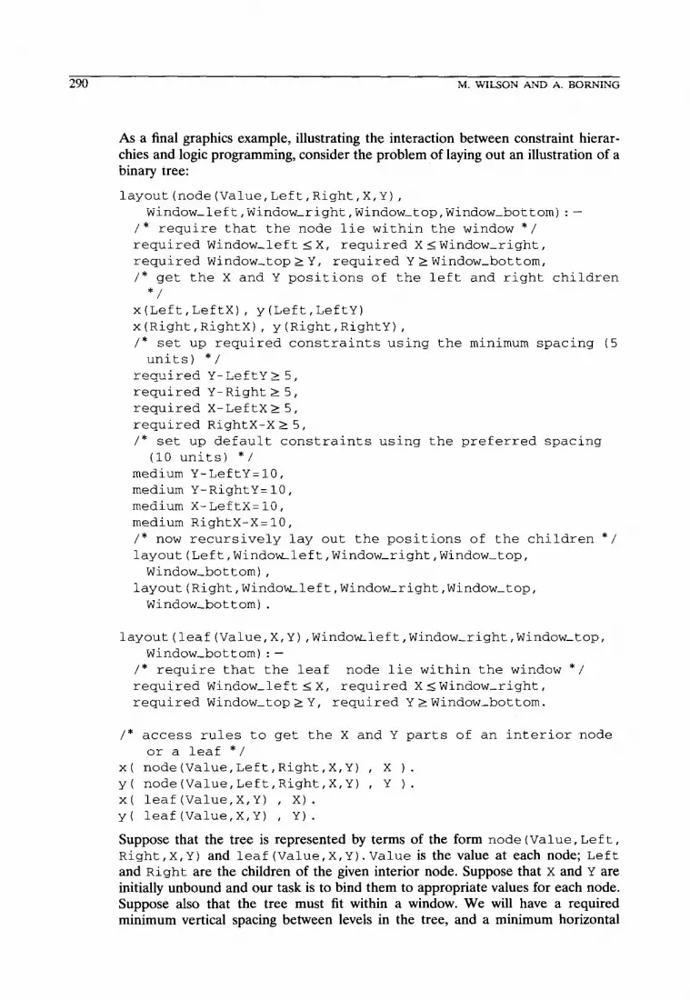
As a final graphics example, illustrating the interaction between constraint hierarchies and logic programming, consider the problem of laying out an illustration of a binary tree:

layout(node(Value,Left,Right,X,Y),

Window_left,Window-right,Window-top,Window-bottom):-

/" require that the node lie within the window */

required Window-left<X, required XIWindow_right,

required Window-top>Y, required Y>Window_bottom,

/* get the X and Y positions of the left and right children

*/ x(Left,LeftX), y(Left,LeftY)

x(Right,RightX) , y(Right,RightY),

/* set up required constraints using the minimum spacing (5

units) */

required Y-LeftY25,

required Y-Right? 5,

required X-LeftX25,

required RightX-X25,

/* set up default constraints using the preferred spacing

(10 units) */

medium Y-LeftY=lO,

medium Y-RightY=lO,

medium X-LeftX=lO,

medium RightX-X=10,

/* now recursively lay out the posit ldren */ ions of the chi

layout(Left,Windoxleft,Window-right,Window-top,

Window-bottom),

layout(Right,Windomleft,Window_right,Window-top,

Window-bottom).

layout(leaf(Value,X,Y),Windo~left,Window_right,Window-top,

Window_bottom):-

/* require that the leaf node lie within the window */

required Window-left IX, required XsWindow-right,

required Window_top>Y, required Y>Window_bottom.

/* access rules to get the X and Y parts of an interior node

or a leaf */

x( node(Value,Left,Right,X,Y) , X ).

y( node(Value,Left,Right,X,Y) , Y ).

x( leaf(Value,X,Y) , X).

y( leaf(Value,X,Y) , Y).

Suppose that the tree is represented by terms of the form node (Value, Left , Right,X,Y) and leaf(Value,X,Y).Value is the value at each node; Left

and Right are the children of the given interior node. Suppose that x and Y are initially unbound and our task is to bind them to appropriate values for each node. Suppose also that the tree must fit within a window. We will have a required minimum vertical spacing between levels in the tree, and a minimum horizontal


spacing between the parent and the left and right children, and also somewhat larger preferred spacings. A recursive layout rule will set up the appropriate constraints on the x and Y variables in each node: hard constraints that enforce the minimum spacing restrictions and that force the entire image of the tree to lie within the window, and soft constraints that try to lay out the nodes using the preferred spacing. The tree will be layed out using the preferred spacing if possible; otherwise it will be squeezed down as needed to fit in the window. (The most appropriate comparator for this application would be least-squares-better, which would distribute the compression over all the spacings.) Of course, if the tree cannot be layed out so that the required constraints are satisfied, the goal would fail.

4.2. Planning and Scheduling

Here is a sample HCLP(9) program that determines when a group of people can meet and that will also find a meeting room for them:

free(alan,6,8). free(bjorn,8,9). free(john,ll,l2). free(molly,l0,12). free(conference_room,8,10). room(conference-room).

find_times([PersonlMorel,Start,End):- find_time_for_one(Person,Start,End), find_times(More,Start,End).

find_times([],Start,End) .

find_time_for_one(Person,Start,End):- free(Person,StartFree,End_Free), medium Start-FreesStart, medium End_Free>End.

find_room(Room,Start,End):- room(Room), free(Room,Start-Free,End-Free), strong StarLFreesStart, strong End-FreerEnd.

The following query finds a one-hour meeting time for Alan, Bjorn, John, and Molly:

?-find_times([alan,bjorn,john,mollyl,S,E), find_room(Room,S,E), required E-S=l.

The program processes the list of participants, accumulating constraints on the start and end time for each. For each person, medium constraints are added that


the person be free during the meeting time. Also, we need a meeting room; the program looks for a meeting room, and adds a strong constraint that the room be free during the proposed time. (We did not make it a required constraint, because perhaps we can persuade the other users of the room to move their meeting, or there may be some other constraint on everyone’s time that takes priority over the room being free, such as a fire drill.) The program will succeed in finding a meeting time regardless of how solutions are chosen, because none of the conflicting constraints is at the required level.

If we are only considering each constraint individually, as with the local and regional comparators, then the program will return as its answer all one-hour intervals between 8:00 and 10:OO. (All of these intervals satisfy the required constraint that the meeting last an hour and the strong preference that the conference room be free. Because we cannot satisfy everyone’s personal preferences regarding the meeting time, in this case we do not try to distinguish further among the solutions.) For this program, the regional comparators return the same answers as their local counterparts. However, if we add a weaker constraint, for example one that weakly prefers meetings close to lunch time, the regional answers may be further refined and some of these solutions may be rejected. (For the local comparators, the set of solutions would not be affected by this change.)

Weighted-sum-metric-better also selects all one-hour intervals between 8:00 and 10:OO. However, if we were to add another person to the list of attendants for the meeting, say someone who was free from 9:00 to lO:OO, then weighted- sum-metric-better would select the hour beginning at 9:O0. By minimizing the sum of the errors, this comparator attempts to “make the most people happy.”

Weighted-sum-predicate-better yields an 8:00 meeting time because that is the time that satisfies the most people (one, in this case> while still satisfying the stronger meeting time constraints.

Least-squares-metric-better chooses 8:45 as the desired meeting time. This comparator is similar to weighted-sum-metric-better in that the total error is being considered in finding a solution, but because the errors are being squared, outlying constraints (such as Alan’s early meeting preference) tend to skew the results.

The answer using worst-case-metric-better is 8:30 because this is the time that produces the smallest single error of any of the times from 8:00 to 10:OO. In effect, no one person will be too put out by the results using this comparator.

We can conceive of scenarios where each of these solutions is most desirable. Normally, we might prefer to use a predicate comparator for scheduling meetings, so that we do not find ourselves meeting at strange times that are no good for anyone. Yet in some situations, such as deciding what time of year to meet, it is important to take exact error into account.

4.3. Document Formatting

In this example, we want to lay out a table on a page in the most visually satisfying manner. We achieve this by allowing the white space between rows to be an elastic


length. It must be greater than zero (or else the rows would merge together), yet we strongly prefer that it be less than 10 (because too much space between rows is visually unappealing). We do not want this latter constraint to be required, however, because there are some applications that may need this much blank space between lines of the table. We prefer that the table fit on a single page of length 30 (units). There is a weak default constraint that the white space be 5, that is if it is possible without violating any of the other constraints. Finally, there is another weak constraint specifying the default type size:

table(PageLength, TypeSize,NumRow,WhiteSpace):-

required (WhiteSpace+TypeSize)* NumRow=PageLength, required WhiteSpace> 0,

strong WhiteSpace<lO,

medium PageLengths 30,

weak WhiteSpace=5,

weak TypeSize=ll.

If we use a predicate comparator, then if the medium constraint cannot be satisfied and the table takes up more than one page, the weak constraint will be satisfied, resulting in WhiteSpace = 5. However, if we use a metric comparator, spacing between the rows will be as small as possible to minimize the error in the PageLength constraint at the medium level.

We can avoid this behavior by demoting the medium constraint to a weak one so that the size of the type, the white space between rows, and the number of pages all interact at the same level in the hierarchy. Weighted-sum-better will character- istically choose the solution that minimizes the error for the majority of the constraints, while worst-case-better finds the middle ground.

As demonstrated by this example, it may not be apparent until some experimen- tation has taken place what even constitutes a suitable solution. The user may need to experiment with using various comparators (or even combining them for different parts of the problem) and with different strengths on given constraints to determine the desired solution.

4.4. Financial Examples

The CLP(%) rules for computing mortgage interest [30] provide a good illustration of the power of the language, because they can be used in a variety of ways (to compute the monthly payment given the other information, to find the symbolic relation between the principal and monthly payment, and so forth):

mortgage(Principa1, Months, Interest, Balance, MonthlyPmt):-

Months> 0,

MonthsIl,

Balance+MonthlyPayment=Principal*(l+Interest).

mortgage(Principa1, Months, Interest, Balance, MonthlyPmt):-

Months>l,

mortgage(Principal*(l+Interest)-MonthlyPayment,

Months-l, Interest, Balance, MonthlyPayment).


We can of course use the same rules in HCLP(9) and also add preferential constraints. For example, the following goal uses the standard CLP(9) rule to find a symbolic constraint relating the Principal and the MonthlyPayment for a conven- tional fixed-rate 30 year mortgage at 1% interest per month, and then gives preferences regarding the maximum monthly payment and the minimum amount borrowed. For the given goal, the two preferences can be satisfied simultaneously:

?-mortgage(Principa1, 360,0.01,O,MonthlyPayment),

strong Principal2100000, strong MonthlyPaymentIlSOO.

When the monthly payment falls between $1500 and $1028.61, then both of the strong constraints can be satisfied, However, if the query changes to

?-mortgage(Principa1, 360,0.01,O,MonthlyPayment),

strong Principal2100000, strong MonthlyPaymentSlOOO.

then the strong constraints cannot be satisfied at the same time, i.e., given the constraints on the interest rate and the life of the loan, a buyer could not purchase a house for $100,000 or more and keep the monthly payment below $1000. In this case, the single solution found by weighted-sum-metric-better would yield a monthly payment of $1028.61 for a loan of $100,000. (No other solution has as small a combined error, because a given change in the principal results in a much smaller change to the monthly payment.) Worst-case-metric-better and least-squares- metric-better give solutions that are very close (within a dollar) to this one.

As a second financial example, consider the use of HCLP(9) for implementing an options trading analysis system such as O.T.A.S. 1311. Option-based investment strategies can be tailored to fit the profile of a specific investor and to take into account currently prevailing market conditions. Mathematical models of market behavior define the parameters that are used to express the characteristics of those strategies. Typically these strategies are described by sets of constraints on selected parameters. It is possible that, given the current market conditions, there will be few or no solutions. To avoid the situation where an exhaustive search fails, because we cannot satisfy all of the constraints, we can weaken the strength of some of the constraints that were previously required. The more important a constraint, the greater the strength it is given.

5. INTERHIERARCHY COMPARISON

In some applications, it is useful to compare not just solutions to a given constraint hierarchy, but also solutions arising from several different hierarchies. Let us return to a simple scheduling problem similar to that given in Section 4.2, but uncomplicated by the choice of a meeting room. That is, we only wish to select a meeting time for two people and we have a room that is available all day:

free(nate,8,12).

free(nate,l8,21).

free(callie,l7,21).

free(conference_room,8,21).

room(conference_room).

In this example, Nate is free at two separate times of the day-once before noon and once from early evening on. An HCLP(9) program using the weighted-sum-


metric-better comparator would produce two answers for the query

?-find_times([nate,callie],S,E),

find-room(Room,S,E),

required E-S=l.

The first answer, meeting for an hour sometime between noon and 5:00 p.m., stems from the first rule selection for Nate. The second answer, meeting for an hour sometime between 6:00 p.m. and 9:00 p.m., arises from the second rule choice for Nate. In effect, two hierarchies are constructed here: one using the first and the other using the second free time for Nate. It seems evident to a person trying to solve this problem that the second answer is really the “best” in that it completely satisfies both people’s preferences. One way to achieve this answer using the constraint hierarchy theory is to allow a comparison between the solutions arising from the first hierarchy and those arising from the second with respect to how well a solution satisfies its own hierarchy. (Clearly we would not want to compare say 1330 p.m. and 6:00 p.m. using just one of the hierarchies. 1:00 p.m. is not even a solution to the second hierarchy!) In 1811 the original constraint hierarchy theory was extended to allow for just such interhierarchy comparisons. In what follows, the definitions from Section 2 are similarly extended.

A solution to a set of constraint hierarchies A will consist of a set of valuations for all the free variables in A. In all cases where A consists of a single hierarchy, the following definitions are equivalent to those given in Section 2:

where IZ is the max of the number of levels in H and J]

We first define the set SoA of valuations that satisfy all the required constraints in some hierarchy in A. Each valuation 8 in Sab is annotated by the hierarchy H that it satisfies. Using SoA, we define the set S, as before, only now we are comparing across different hierarchies. Thus we eliminate potential valuations that are worse than some other from any hierarchy in A.

Extending the definition in this way gives rise to some nonmonotonic properties. These are discussed in [Bl].

We should point out that interhierarchy comparison only makes sense with respect to the global comparators where the errors at each level in the hierarchy are conglomerated, and it is therefore reasonable to compare those errors arising from completely different sets of constraints. For the local and regional comparators, on the other hand, ordering vectors of errors from different constraints via the cg relation seems meaningless. For this reason, interhierarchy comparison is only defined for global comparators.

There are many other examples of programs where interhierarchy comparison yields the most intuitive answers. Aside from the restriction to global comparators discussed previously, there are two other reasons why an HCLP interpreter restricts its comparisons to single hierarchies. The first and most important reason


has to do with efficiency. Consider the program fragment

f(X):-g(X), medium X<O.

g(l).

g(X) : - g(X- 1).

There is nothing in the definition of the global comparators that prevents the set of hierarchies A from being infinite. In practice, this can occur when rules are recursive, as demonstrated in the foregoing program. In general, an interpreter using interhierarchy comparison would have to construct all the hierarchies arising from alternate rule choices, collect all the valuations that satisfy the required constraints in those hierarchies, and then compare them to find the solution set. In cases where the set of hierarchies is infinite, such a procedure will not return unless judicious pruning of the search tree allows infinite branches not to be traversed. For programs such as the preceding one, in general there is no way to avoid an infinite search for the best solution. (To avoid such a search we would potentially need to solve the halting problem.) If, however, the medium constraint in the first rule were altered to medium X > 0, then all valuations for X that satisfied the predicate g would also satisfy all the constraints in their respective hierarchies. We would want an efficient implementation to make use of such information so that answers could be produced one at a time.

The second justification for preferring single hierarchy comparisons is for programs where we want all possible answers to a query. Consider the following program that attempts to characterize mealtimes:

free(callie,S,E):- strong S218.

mealtime(breakfast,S,E):-S26, E<lO, E-S=0.5

mealtime(lunch,S,E):-ST12, E(13, E-S=l.O

mealtime(dinner,S,E):-S217, E120, E-S=1.5

eat(Person,S,E):-

mealtime(Meal,S,E),

free(Person,S,E).

The first rule states that Callie is free all day, but that she strongly prefers that anything that is planned occur after 6:00 p.m. This may be reasonable for scheduling a get-together, but if we use this in conjunction with planning mealtimes, interhierarchy comparison will have Callie skipping breakfast and lunch. Instead, using the more standard intrahierarchy comparisons, Callie’s preference would have no effect on the other mealtimes (using a predicate comparator), but it would move the dinner hour to after 6:00 p.m.

6. A MODEL THEORY FOR HCLP

In 1671, the notion of preferred models is introduced as a way to represent the meaning of certain nonmonotonic logics. Some subset of the models of a set of formulas can be selected as the “preferred” models, thereby defining a particular nonmonotonic logic. A preference relation c is used to partially order the models.


M, CM* denotes that the interpretation M, is preferred over the interpretation M2. A preferred model for a sentence A is an interpretation M such that M K A and there is no other interpretation M’ such that M’ E A and M’ c M. There are many possible methods of ordering models, and various logics can be characterized by defining, different preference criteria.

There has been other work, specifically in the area of logic programming with negation, that deals with the notion of a canonical model for a particular logic program. There have been various methods used for defining what a canonical model should be (see [l, 27, 5311, but the intention is always that the canonical model represent exactly those queries that have “yes” answers in the program. A canonical model for a program P is defined in several of these approaches by selecting some variant of P, P’, and using a minimal model for P’. Although we might also wish to adopt the concept of a canonical model to represent the meaning of an HCLP program, the idea of ordering models via a preference relation fits more closely with the notion of comparators than does the variation of the canonical model approach.

In this section, we first give a very short review of CLP theory and then discuss some of the aspects of HCLP that require us to use the notion of extended models. We then use these extended models with a preference relation to define the preferred models of HCLP programs. Finally we show how this framework can be altered to give a formal semantics for HCLP programs with interhierarchy comparison.

6.1. Review of CLP Model Theory

In 1341 a model is defined for CLP programs. First, the base of a program is defined as

P base = {P(xl~x,~-~~ x,) 8 I p is a predicate in KI, and

8 is a valuation for the variables x1,. . . , xn}.

Then a model of a program P is defined as a subset Z of Phase such that for every rule in P,

A +B,,B,,...,B,, C,

and for every valuation 8 that satisfies the constraints in C,

(ZV,B,~,..., B,B} cZ implies AOEZ.

6.2. An Extended Model

A model for an HCLP program must contend with the nonrequired constraints. This can be quite complicated, because any reading of the program that does not in some way take error into account will not capture the intended meaning of the constraint hierarchy. In fact, unlike CLP, we cannot determine whether a particular valuation satisfies a nonrequired constraint unless it is viewed in the context of the entire hierarchy. It is the disorderly property of constraint hierarchies 1811 that gives rise to this phenomenon. In essence, this property states that the solution to a constraint hierarchy, H, may be completely disjoint with the solution to the


hierarchy H U {lc), where 1 is a label and c is a constraint. This means that we cannot look at error in isolation-the meaning depends on how rules are combined. To handle this, we define an extended model for P that consists of tuples of predicates and error sequences. If we consider the predicates in the extended model without the error sequences, then we simply have a model for P minus all of the nonrequired constraints, i.e., a CLP program. Intuitively we want to start out with a model for the underlying CLP program and then use the comparators to define a preference relation that utilizes the error sequences.

Proceeding as described before yields a model theory for HCLP with interhierarchy comparison. To first give a model theory for intrahierarchy, or single hierarchy comparison, we need to complicate the notion of an extended model so that we can isolate all tuples in the extended model arising from the same derivation. It is not sufficient to look at a valuation in isolation, because its being in the solution set depends on how well it satisfies the hierarchy in comparison to other valuations that also satisfy the required constraints and that arise from the same derivation. To clarify this point, consider the following HCLP(5%‘,9AG’) (locally-metric-better) program (the numbers on the left are not part of the program; they will be used later to refer to particular rules):

1 squid(X):-mollusc(X), weak X210.

2 mollusc(X):-required X=11.

3 mollusc(X):-required X53.

The query ? - squid (x) has two answers: one that maps X to 11 and one that maps X to 3. An extended model would include the tuples (mollusc(ll),[ I), (squidW, [Dll>, and (squidW, W311), among others. (Note that [ ] is the empty error sequence.) If we compare the tuples (squid(ll),[[O]]) and (squid(3),[[7]]), then we would wrongly eliminate squid(3) from the solution set because [[Oil < [[711. On the other hand, if we look at the tuple (squid(2),[[8]]) by itself, we will not recognize that there is another valuation, namely, that which maps X to 3, whose error is less than the error for the valuation that maps X to 2. To avoid false comparisons, while also ensuring that the right valuations are compared, the extended model is made up of a set of sets, rather than a single set. Each set corresponds to a particular constraint hierarchy and each valuation in a set can be compared with every other valuation in the same set. Numbering the rules and subscripting the subsets of the extended model are record-keeping devices used to differentiate the different subsets.

Although this appears to diminish the declarative nature of the model theory, it is a necessary extension. Intrahierarchy comparison based as it is on a single derivation is in some sense inherently operational. Yet we find it useful to present a model theory for several reasons. First, it is helpful to be able to make comparisons with the more standard CLP model theory. It turns out that HCLP programs without nonrequired constraints yield extended models whose similarity to the models for the equivalent CLP programs are evident (which is as it should be!). Second, one of the main motivations for using single hierarchy comparisons is efficiency. The extended models for HCLP programs with interhierarchy comparison are declarative in nature and, with the exception of the error sequences, are identical to models for the equivalent CLP programs. Third, the model theory enables us to consider the comparators as preference relations. This is a quite useful view and it allows us to see HCLP in relation to nonmonotonic logic. The


constraint hierarchy in conjunction with logic programming allows us to prune the set of preferred valuations.

Let a numbered program be a program such that every rule has a unique number. Let the extended base of a program P be defined as

P c&base = {(P(-+**Y@P~)I

p is a predicate in II, and

0 is a valuation on the variables x, , . . . , x, and

R is an error sequence}.

Let the result of interleaving error sequences R,, R,, . . . , R,, each of length n, be anewsequenceoflengthmn,denotedbyR,@R,@.**@R,.If R,=[rI,,...,rI.I, R, = [rzl,. . ., rznl,. . . , and R,,, = [rml,. . . , rmn], then

R,@R,@ *-- @R, =[r,1,r2,,...,rml,...,rln,r2n ,..., r,,,,].

Let p(B) denote the power set of the set B. Let an extended model for a program P be a subset Z of @(Pext_base) such that for every rule in the numbered program P,

(9 A +B,,B,,...,B,,ff,

and for every valuation 8 E S(H,),

(B,~,R,)EZ,,(B,~,R,)EZ, ,..., (B,~,R,)EZ,, forZ,,Z, ,..., Z,EZ,

implies

(~8, R, teR, e - @R, @ [E(H,8),E(H,e),...,E(H,e)]) EZj,

for iIjIm.

Let the minimal extended model for a program P, denoted MM,, be an extended model for P such that there is no other extended model A4; for P such that A4; CMM,.

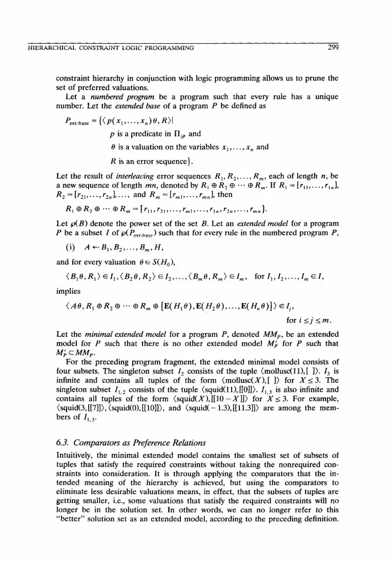
For the preceding program fragment, the extended minimal model consists of four subsets. The singleton subset Z2 consists of the tuple (mollusc(ll), [ 1). Z3 is infinite and contains all tuples of the form (mollusc(X), [ I> for XI 3. The singleton subset I,, z consists of the tuple (squid(ll), [[O]]). I,,, is also infinite and contains all tuples of the form (squid(X),[[lO -Xl]> for XS 3. For example, (squid(3,[[71]), (squid(O), [[lOI]>, and (squid( - 1.31, [[11.3]]) are among the members of I,,,.

6.3. Comparators as Preference Relations

Intuitively, the minimal extended model contains the smallest set of subsets of tuples that satisfy the required constraints without taking the nonrequired constraints into consideration, It is through applying the comparators that the intended meaning of the hierarchy is achieved, but using the comparators to eliminate less desirable valuations means, in effect, that the subsets of tuples are getting smaller, i.e., some valuations that satisfy the required constraints will no longer be in the solution set. In other words, we can no longer refer to this “better” solution set as an extended model, according to the preceding definition.


Therefore, we will define preference relations over subsets of P(Z’~~~_+_) (extended interpretations), rather than over extended models. Let g be a comparator, and let Z and Z’ be extended interpretations for a program P. Let S and S’ be members of I and I’, respectively, such that S and S’ have identical subscripts. Then I’ cg Z if (1) S’cS and (2) if 3(p(x,,..., x,)u,R,) E S,E S’, then Xp(x ,,..., x,)0,&) ES’ and G(R,) <a G(R,).

6.4. Mapping the Extended Model to a Standard Model

Our goal is to define a model for an HCLP program P using the comparator g. We still need to define a set that represents the answers to a query. First we define the pruning operator that simply removes the error sequences from an extended interpretation and collapses the subsets into a single set. Let Z be an extended interpretation. Then

prune(Z) = (p(x,,...,x,)8(3SEZ

A(p(x,,..., x,)8,&) ES}.

Now we say that prune(M) is a preferred model for a program P using the comparator g if (1) MM, is an extended minimal model for P using g and M cg MM, and (2) there is no other extended interpretation M’ such that M’ cg M.

If a program contains no nonrequired constraints, then there is an equivalent CLP program that can be produced by simply omitting the required label from each constraint. In this case, the extended minimal model Z will consist of sets of tuples whose second elements are empty error sequences. Therefore, none of these empty sequences will dominate any other sequence in the same set and no ground atoms will be eliminated in the preferred model M. For programs with required constraints only, M consists simply of all the first elements in the tuples in the sets in I.

6.5. A Model for Inter-hierarchy Comparison

With only a small change, the extended model theory can be altered to give a semantics for interhierarchy comparison. Rather than dividing the extended model Z into sets, the extended model for interhierarchy comparison consists of a single subset of Pext_base.

Let an extended model for a program P using interhierarchy comparison be a subset Z of Pext_base such that for every rule A + B,, B,, . . . , B,, H in P, and for every valuation 13 E S(ZZ,),

(B,e,R,),(B,8,R2) ,..., (B,O,R,) EZ

implies

where @ is the interleave operator defined in Section 6.2. A minimal extended model is defined in the same way. The preference relation

on extended interpretations is also a bit simpler than the one used for single


hierarchy comparison. Let g be a comparator, and let I and I’ be extended interpretations for a program P using interhierarchy comparison. Then I’ cg Z if (1) I’ cl and (2) if 3(p(x,,..., x,)u,R,)EZ, @Z’,then 3(p(x, ,..., x,)O,R,)E I’ and G(R,) <g G(R,).

Finally, we need to redefine the prune operator for interhierarchy comparison:

prune(Z) = (p(xI,...,x,)Ol

(P(X,,..., x,)0,&) EZ}.

Then, as defined for intrahierarchy comparison, prune(M) is a preferred model for a program P with comparator g using interhierarchy comparison if (1) MM, is an extended minimal model for P using g and Mc~ MM, and (2) there is no other extended interpretation M’ such that M’ cg M.

7. A FIXED-POINT SEMANTICS

To provide a fixed-point semantics for HCLP (without interhierarchy comparison), the Tp function is defined that maps sets of sets of tuples of the form (A 0, R) into sets of sets of tuples that can be formed via the application of a single rule in the program P. A single set represents derivations that can later be compared because they are constructed from the same constraint hierarchy.

More formally,

r, : @7(rn( Pext-base) > -+ @Cd Pext-base > 1.

For 1 c dPcxt_base 1,

T,(I) = (Fl

A +- B, , B, , . . . , B,, Hisarulein P,and

F={(AO,R)l

(40, R,) EZ~,

(Z&O,&) EZ~,

Let

(B,O,R,) EL,,

for I,, Zz, . . . , Z,,, E I, and

OES(Ho), and

R=R, $R,e .-- @R, e3 [E(H,o),E(H,o),...,E(H,~)])

1.

TpTw= fi T;(0), i= 1


Although Tp t w is a fixed point, the valuations contained in its sets still need to be compared. The S best operator is essentially a filter that eliminates those valuations whose combined error vectors are larger than some other valuation in the same subset. Sbest computes the preferred solutions of the set I. Let

%_st(Z) = (A@1

31’ E Z and

il(AB,R,)EZ’and

T~(Au,R,)EZ' suchthat

G(R,) <g G(R,)]*

If a program contains no nonrequired constraints, then Tp r w will consist of sets of tuples whose second elements are empty error sequences. Therefore, none of these empty sequences will dominate any other sequence in the same set and no ground atoms will be eliminated in Sbest(TP t w>. For programs with required constraints only, Sbest(TP t > w consists simply of all the first elements in the tuples in the sets in I.

7.1. A Fixed-Point Semantics for Inter-hierarchy Comparison

We can also alter the definition of Sbest only slightly to achieve a fixed-point characterization for interhierarchy comparison, in much the same way as for the model theory. Z now consists of a single subset of &?ext_base). Then we redefine the mapping function Tp as

TP : @3( Pext-base) * @7( ‘ext-base) *

For 1 G Pext_base_,

T,(Z) = {{(AfhRN

A +Bl,BZ,..., B,,Hisarulein P,and

(B,O, R,) EZ,

(B,@,R,) EZ,

(&,O,R,,,) ~1,

OES(ZZo), and

R=R,@R,@ 1-0 @R,,, as [E(H,8),E(H,8),...,E(ZZ,$)])

1.

Similarly, we redefine Sbest as

Sbest(z) = 1 Ael

(Ati,R,)~Zand

~XAa,R,)~Zsuchthat

G(R,) <s G(R,)}.


In this definition, the mapping Sbest is not monotonic, as is also discussed in [811.

8. RELATIONS BETWEEN THE OPERATIONAL, MODEL-THEORETIC, AND FIXED-POINT SEMANTICS OF HCLP

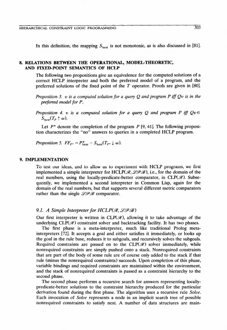
The following two propositions give an equivalence for the computed solutions of a correct HCLP interpreter and both the preferred model of a program, and the preferred solutions of the fixed point of the T operator. Proofs are given in [SO].

Proposition 3. v is a computed solution for a query Q and program P iff Qv is in the preferred model for P.

Proposition 4. v is a computed solution for a query Q and program P ifl Qv E S,,est(TP t ~1.

Let P* denote the completion of the program P [9, 411. The following proposition characterizes the “no” answers to queries in a completed HCLP program.

Proposition 5. FF,. = Pease - Sbest(TP* J. 0).

9. IMPLEMENTATION

To test our ideas, and to allow us to experiment with HCLP programs, we first implemented a simple interpreter for HCLPM?, 59990, i.e., for the domain of the real numbers, using the locally-predicate-better comparator, in CLP(91. Subse- quently, we implemented a second interpreter in Common Lisp, again for the domain of the real numbers, but that supports several different metric comparators rather than the single _%9B comparator.

9.1. A Simple Interpreter for HCLP(S?, _5?X@B>

Our first interpreter is written in CLP(B?), allowing it to take advantage of the underlying CLP(9’) constraint solver and backtracking facility. It has two phases.

The first phase is a meta-interpreter, much like traditional Prolog meta- interpreters [721. It accepts a goal and either satisfies it immediately, or looks up the goal in the rule base, reduces it to subgoals, and recursively solves the subgoals. Required constraints are passed on to the CLP(9) solver immediately, while nonrequired constraints are simply pushed onto a stack. Nonrequired constraints that are part of the body of some rule are of course only added to the stack if that rule (minus the nonrequired constraints) succeeds. Upon completion of this phase, variable bindings and required constraints are maintained within the environment, and the stack of nonrequired constraints is passed as a constraint hierarchy to the second phase.

The second phase performs a recursive search for answers representing locally- predicate-better solutions to the constraint hierarchy produced for the particular derivation found during the first phase. The algorithm uses a recursive rule Solve. Each invocation of Solve represents a node in an implicit search tree of possible nonrequired constraints to satisfy next. A number of data structures are main-


tained by each invocation of Solve, including Answer (a list of unlabeled constraints that represent the answer computed so far) and Untried (a list of labeled constraints that have not yet been dealt with). Let s be the strongest strength of the constraints in Untried. For each constraint c in Untried with strength s, Solve appends c to the current answer, refines Untried by removing constraints that either have become unsatisfiable by the assumption that c holds or that are implied by the current answer, and then recursively calls itself with the remaining untried constraints. The base case is reached when the hierarchy is empty.

Each leaf in the implicit search tree represents an answer to the goal. Upon request, the interpreter will backtrack to find alternate answers. These can arise in two ways. First, it is possible that the constraint hierarchy produced by the current choices of rules has more than one answer. Second, it is also possible that a goal can be satisfied in more than one way at the rule level: by using different rules to solve a goal, a new constraint hierarchy may be obtained. All answers to the current hierarchy are given before an attempt is made to resatisfy the goal. There is a unique computation tree associated with every answer, but the answers themselves are not always unique. (The pseudocode for this algorithm can be found in [6].)

Here is a trivial example in HCLP(%“,_JZZ5@) to illustrate the interpreter’s behavior upon backtracking:

banana(X):- artichoke(X), weak X>6. artichoke(X) :-strong X=1.

artichoke(X):-required X> 0, required X<lO, weak X<4.

The first answer to ? - banana (A) is produced by selecting the first of the art ichoke clauses, yielding the hierarchy strong A = 1, weak A > 6. There is a single answer to this hierarchy, namely A = 1. Upon backtracking, the second art ichoke clause is selected, resulting in the hierarchy required A > 0, required A < 10, weak A < 4, weak A > 6. This hierarchy has two answers. The first is 0 <A < 4. Upon backtracking, the second and final answer 6 <A < 10 is then found.

As a result of being implemented on top of CLP(&%‘), the interpreter is small (two pages of code) and clean. However, the second phase is not incremental-rather, it recomputes all the LPB answers for each invocation, instead of incrementally updating its answers as constraints are added and deleted due to backtracking, thus making it not particularly efficient. A second deficiency is that it does not check for duplicate constraints when pushing nonrequired constraints onto the stack. However, because it implements only the LPB comparator, rather than one of the global ones, the only consequence is that a given answer could be produced more than once upon backtracking.

9.2. A DeltaStar-Based Zntelpreter for HCLP(9, * )

This first implementation only supported the locally-predicate-better comparator. However, metric comparators are important for such applications as interactive graphics, layout, and scheduling, because if a soft constraint is unsatisfied, we may nevertheless wish to satisfy it as well as possible by minimizing its error. Global comparators, which consider the aggregate error for the constraints at a given

HIERARCHICAL CONSTRAINT LOGIC PROGRAMMING 30.5

level, are useful as well for such applications. There is also a fundamental efficiency problem, as previously noted, because the interpreter used a batch algorithm to produce its answers rather than an incremental one.

We therefore wrote a second HCLP interpreter, again for the domain of the real numbers, but that supports the weighted-sum-metric-better, worst-case- metric-better, and locally-metric-better comparators. The comparator to be used in a given program is indicated by a declaration at the beginning of an HCLP program. This second interpreter could thus be precisely but verbosely named HCLP(53’, ( WSMB, WCMB, LMB)). (So far we have resisted the name

HCLPM’, ( 1, I, 8~ )>.I An unfortunate consequence of the desire to support metric comparators is that

we could no longer build so simply on top of CLP(3?), because we now care not just whether or not a constraint is satisfied, but also about the error in satisfying it -information not conveniently available from CLP(3). The second interpreter is thus implemented in Common Lisp and has to do much more of the work itself (such as keeping track of backtracking information).

The interpreter uses an incremental algorithm, DeltaStar [21, 221, to find solutions to constraint hierarchies. DeltaStar is actually a family of algorithms, parametrized by an underlying “flat” constraint solver (i.e., one that solves a collection of required constraints). The key procedure that the flat solver must provide is filter:

filter( S : Solution, C : Set of Constraints ) +Solution.

Given an existing solution S, filter returns the subset of S that minimizes the error in satisfying the set of constraints C. (The implementation of this routine effectively defines the comparator.) In addition, the flat solver should provide other entries for efficiently determining if a new constraint is compatible with a current solution (i.e., if the error in satisfying it is 0) and for quickly adding a constraint to a current solution, given a guarantee that the constraint is compatible. A full description of the algorithm (including a large number of optimizations) is given in

1211. DeltaStar manages the incremental addition and deletion of constraints at

different levels of the hierarchy, given the pluggable flat solver. The remainder of the interpreter maintains the database of clauses, backtracking information, and other details.

9.2.1. Using DeltaStar in HCLP(9, * ). In our Common Lisp implementation of HCLP(W, *), the flat solver is the Simplex algorithm, with implementations of filter that support minimizing the weighted sum of a set of constraints, minimizing the maximum error of a set of constraints, and minimizing the pareto-optimal point of a set of constraints, thus implementing weighted-sum-metric-better, worst-case-metric-better, and locally-metric-better, respectively. The class of constraints that can be accommodated is linear equalities and nonstrict inequalities.

To support these comparators, DeltaStar transforms the constraint hierarchy into a series of linear programming problems. In a standard linear programming problem [451, we wish to minimize (or maximize) a linear expression in k real- valued variables x,, . . . , xk, subject to the nonnegativity constraints x, 2 0,. . . , xk 2 0, and also to m additional linear equality or inequality constraints on x,, . . . , xk. The expression to be minimized or maximized is called the objective function.


Reference 45 gives a comprehensive discussion of linear programming theory and algorithms; all of the transformation techniques mentioned in the following para- graphs are discussed in this volume. Our implementation uses code for the Simplex algorithm taken from [521 and translated to Lisp.

In general, the variables in the constraint hierarchy are unrestricted in sign, whereas those in a linear programming problem must be nonnegative. There is a standard technique for handling unrestricted variables in linear programming problems. Each unrestricted variable xi is replaced by the difference of two nonnegative variables x,? and f,:, so that xi =x,f -x,7. We then solve the problem involving the xi’ and x,: variables, and use this solution to find values for the original xi. (This is not a particularly efficient way of handling this situation, but we used it in this prototype implementation because we were not too concerned with efficiency and wanted to use the Simplex code unaltered.)

We now consider the weighted-sum-metric-better comparator. Initially, we minimize the weighted sum of the errors of the H, constraints, subject to the H, constraints. Even after the transformation to handle the variables without sign restrictions, this still is not quite a linear programming problem because the objective function is a weighted sum of absolute values. However, we adapt another standard technique for converting a problem in which the objective function is the weighted sum of absolute values into a linear programming problem. Let c be a constraint in Hi. If c is an equality constraint aixi + .** +a,~, = b, then the error in satisfying c is e = Jaix, + *a* +a,~, - bl. We augment the linear programming program with two new variables e+ and e- (both of which must obey the usual nonnegativity constraints) and add the constraint aixi + ... +a,~, - b = e+ - e-. If the property

e+=O , if e10,

e-= 0, if e 2 0,

is satisfied, then clearly e = e+ + e-. Conveniently, this property is, in fact, satisfied by the solution produced by the Simplex algorithm. Hence, if the weight for constraint c is w, then its contribution to the objective function (the weighted sum of the errors) is we++ we-. If c is an inequality uixi + **- +a,~, I b, then its contribution to the objective function is simply we+. (In this case, we drop the we- term from the objective function. If the inequality is satisfied, then ef will be 0 and e- will be 0 or positive. If the inequality is not satisfied, then e+ will be positive and e- will be 0.) Finally, if c is an inequality uixi + *-a +a,~, 2 b, then its contribution to the objective function is we-.

If this initial linear programming problem (minimizing the weighted sum of the errors of the H, constraints, subject to the H,, constraints) has a unique solution, we are done. Otherwise, we add to the linear programming problem a constraint that the weighted sum of the H, constraints attain its minimum value (as computed in the previous step) and set up another problem where the new objective function minimizes the weighted sum of the errors of the HZ constraints. We continue in this manner for the remaining levels.

For the worst-case-metric-better comparator, we initially minimize the maximum of the weighted errors of the H, constraints, subject to the H, constraints. As before, this is not a linear programming problem, but yet another standard technique is available for transforming it into one. See 1451, page 18.


For locally-metric-better, we consider each constraint in level H, individually in relation to the solution for H,,. Calling Simplex with a particular H, constraint tells us the bounds of the solution with respect to that constraint. When all of the constraints in H, have been processed, the various solutions are combined to yield a solution for level H,. If all of the constraints at that level are satisfied, then this process continues using the constraints at level H2 in relation to the current solution. If some constraint at level H, is not satisfied, then the current solution is the solution to the entire hierarchy.

Filter routines for each of these comparators are defined separately from the logic programming interpreter. A call to filter solves a single level in the hierarchy by minimizing the error of a set of constraints (the current solution) with respect to some other set of constraints (the constraints at some level in the constraint hierarchy). The calling routine in the interpreter uses f i 1 ter to solve the entire constraint hierarchy.

Regionally-metric-better is not currently available. However, it could be added to the implementation by changing the routine that calls filter. The filter for locally-metric-better could be used as is. Rather than stopping iteration through the hierarchy when some constraint cannot be satisfied, as is now done for locally-metric-better, the routine would continue to call filter through all levels of the hierarchy. If, in the future, we wanted to ‘implement least-squares-better, we would define a filter using some nonlinear equation solver. The logic programming interpreter would not need to be revised.

9.2.2. Eficiency Issues. This second interpreter is still a research prototype to test our ideas, rather than being production-quality software. Among its limitations are its restriction to linear equalities and nonstrict inequalities and its efficiency. Regarding the classes of constraints that can be accommodated, clearly it would be desirable to at least provide local propagation for nonlinear constraints, a la CLP(5Y). Regarding efficiency, implementing the interpreter in Common Lisp has made the implementation easier, but slower than writing in a language such as C. In addition, DeltaStar uses only a narrow interface between the flat constraint solver and the rest of the algorithm. Many optimizations would be possible here, following the excellent example of the CLP(5%!) interpreter [361, such as handling simple constraints within the inference engine, providing different solvers for equalities and inequalities, and more efficiently implementing an incremental version of the Simplex algorithm. Nevertheless, the use of the DeltaStar algorithm has aided us in rapidly testing different satisfaction algorithms and comparators. For example, only one person-hour was needed to add the weighted-sum-metric- better comparator once the DeltaStar framework was in place.

The time complexity of the HCLP interpreter is dominated by the cost of the flat constraint solver. In the complexity discussion that follows, we factor out this cost, and represent it simply as p (where p is a function of the number of variables and the number of constraints). The worst-case time complexity of the flat constraint solver we use (the Simplex algorithm) is exponential in the number of variables; however, this behavior is apparently exhibited only by artificially constructed examples. On real problems Simplex performs remarkably well. There are linear programming algorithms whose worst case time is polynomial. Whether such algorithms (Karmarkar’s algorithm in particular) are superior in practical use is still a matter of debate [38].


The cost of solving a particular HCLP(S.‘, * ) query can be broken down into two parts. The first is the cost of finding some solution considering only the required constraints, i.e., the cost of solving the corresponding CLP(S’) program. (Actually, there is a fair amount of overhead in storing the nonrequired constraints and storing solutions in the event of backtracking, but this is also dominated by the cost of calling the flat solver to solve the required constraints.) The second is the cost of solving the constraint hierarchy. Although this is a fairly expensive procedure, it is only done once per answer because there is no need to solve the hierarchy until we know that a particular derivation will not fail. Furthermore, because the algorithm in the current interpreter is incremental, not all of the solution is lost upon backtracking.

Many of the optimizations described will improve the running time of the interpreter with respect to the first type of cost, i.e., that of finding a solution to the required constraints. Using a more efficient flat solver would improve both the cost of finding the set S, and of solving the entire hierarchy.

Consider a particular call to filter, f i 1 t er ( S, c ) , where S and C are sets of constraints. Let u denote the number of variables in S and C. Let c denote the number of constraints in C. Let II be the number of levels used in the HCLP(S?, *) program. Let p be the cost of running the linear programming algorithm in the average case for v variables and c constraints. The cost of f i 1 t er (in the average case> for both weighted-sum-metric-better and worst-case-metric-better is 2up. The cost of filter for locally-metric-better is 2cup. It is often the case that filter will not be called n times. We already saw how this could be in the case of locally-metric-better, but it will also be true if a particular derivation does not include constraints at level n, or in the case that a unique solution is found before processing the constraints at level II. However, assuming that filter is called IZ times, then the cost of solving the hierarchy is 2nup for weighted-sum-metric- better and worst-case-metric-better, and 2ncup for locally-metric-better.

9.2.3. Inteructiue Graphics. The HCLP(S’, *) interpreter includes some evalu- able predicates for performing input and graphical output, so that we can use HCLP(S, *) for interactive graphics applications. For example, there are predicates for getting the mouse position and button state, and for drawing lines, circles, placing text, and so forth. The interpreter makes the appropriate calls to Garnet routines to perform the needed actions. (Garnet [47] is a user interface toolkit, written in Common Lisp and using X windows.)

10. RELATED WORK

As described in the introduction, HCLP builds on the CLP scheme [lo, 341. Because HCLP is also a general scheme, it should be possible to implement HCLP languages for any of the domains, such as Booleans, finite domains, or trees, supported by existing CLP languages (e.g., [ll, 14, 35, 36, 61, 69, 77, 7911.’

A number of CLP languages, for example CHIP [14, 771, include a minimize operator. If an a priori lower bound B on the value of Vur is known, then a call

‘Regarding Echidna [69], we should note that some of its constraint solving techniques make use of a hierarchy, but their meaning is quite different than the one we use here. In the case of Echidna, a hierarchy refers to a taxonomy or a structuring of a discrete domain into subsets with similar properties. This allows the system to use a more efficient arc consistency algorithm.


minimize (Var) could be replaced by a soft constraint medium Vur = B.2 HOW- ever, if an a priori bound is not known, then this simulation would not work. Reference 5 describes how the constraint hierarchy theory can be extended to include objective functions. We could similarly extend an HCLP language to include objective functions explicitly, which would handle minimize directly (module the footnoted comment).

It is also useful to consider the relation between soft constraints and objective functions from the other point of view: of expressing HCLP languages in a CLP language with a minimize operator. The latter sort of language would be a very convenient one in which to write an HCLP interpreter. The technique would be similar to that used in our first HCLP interpreter, which was written in CLP(g) (Section 9.1). However, rather than just the locally-predicate-better comparator, we could implement other comparators as well in such an interpreter. For example, to implement weighted-sum-better, we would first reduce the goal, satisfying the hard constraints, and accumulating the soft constraints. We would then minimize the value of an expression that was the weighted sum of the errors of the constraints at the strongest nonrequired level (using the minimize operator), then the weighted sum of the errors of the next level, and so forth.

The cc family of languages [58, 591 generalizes the CLP scheme to include such features as concurrency, atomic tell, and blocking ask; up to this point we have not dealt with these additional issues in the HCLP framework.

Maher and Stuckey [42] give a definition of constraint hierarchies similar to the one in this paper. In their definition, presolutions for hierarchies perform the same function as the set S, does in our formulation. Then rather than using the E and G functions, Maher and Stuckey define a premeasure that maps presolutions and sets of constraints to some scale. The resulting sequences can then be compared via a lexicographic ordering.

Satoh [60] proposes a theory for constraint hierarchies using a meta-language to specify an ordering on the interpretations that satisfy the required constraints. The theory is quite general and can accommodate all of the comparators described in Section 2. However, because it is defined by second-order formulae, it is not in general computable. In subsequent work [62, 631, Satoh and Aiba present an alternative theory that restricts the constraints to a single domain _!Z, so that they can be expressed in a first-order formula. This theory is similar to the one presented here, with the following differences: (1) Only the locally-predicate-better comparator is supported, (2) the semantics of constraint hierarchies (as opposed to the semantics of HCLP) is described model theoretically rather than set theoretically, and (3) the class of constraints is generalized from atomic constraints to disjunctions of conjunctions of atomic constraints, i.e., constraints of the form

(Cl1 A Cl2 A *** A &,) v (C2, A C22 A ..* A cZn2) V -** V(c,, A c,,,~ A *-. A CT,,,).

Satoh and Aiba embed such constraints in the CLP language CAL [61] to yield an HCLP language CHAL [62, 631. CHAL includes two constraint solvers: an alge-

*Actually, the simulation is not quite precise. Consider the CHIP goals x > 0, X I 10, minimize(X), minimize(O-x) and X20, X510, minimize(O-x), minimize(x). Thesewould give X = 0 and X= 10, respectively. However, the corresponding HCLP goals required X > 0, se- quired X 5 10, medium X=0, medium X=10 and required X 2 0, required X 510, medium X=10, medium X= 0 would both yield the same answers: for example, the two answers X= 0 or X= 10 for locally-predicate-better and the single answer X = 5 for worst-case-better and least-squares-better.


braic constraint solver for multivariate polynomial equations, which uses Buch- berger’s algorithm to calculate Griibner bases, and a Boolean constraint’solver for propositional Boolean equations, which uses an extension of Buchberger’s algorithm. Satoh and Aiba give examples illustrating each of these domains: a meeting scheduling problem and a gear design problem, respectively. In each case, both required and soft constraints are used. They also describe an algorithm for finding the locally-predicate-better solutions to a hierarchy, which improves on our algorithm discussed in Section 9.1 by avoiding redundant calls to the solver. It finds solutions essentially by computing maximally consistent subsets of the soft constraints. However, this algorithm is a batch solver, in contrast to the DeltaStar-based incremental algorithm (Section 9.21, and thus must recompute its answers from scratch after every change to the set of constraints due to an alternate rule choice. Finally, it should be mentioned that the characterization in [62] states the definition of the set of solutions for a given constraint hierarchy in model-theoretic rather than set-theoretic terms, but does not deal with the interactions between rule choice and constraint hierarchies. We define constraint hierarchies and their solutions using sets, but describe the meaning of HCLP programs using both a model theory and a proof theory.

Ohwada and Mizoguchi [50] discuss the use of logic programming for building graphical user interfaces. Default constraints are instrumental in this application because often only an incomplete specification of an object is given, yet complete information is needed to display a picture. Defaults provide a mechanism whereby information can be assumed in order to specify an object fully, yet it can be overridden, if necessary, as further information becomes known. Rather than a single default level, a hierarchy of default constraints is used to avoid obtaining multiple, equally plausible solutions (also known as the multiple extension problem). The hierarchy is implemented using the negation-as-failure rule, i.e., if the negation of a constraint is not known to hold, then the constraint can be assumed to be true. A problem with this approach is that it then becomes necessary to list all possible conflicts when a rule is being written in order to avoid inconsistencies. In HCLP, the need for consistency is assumed and there is no need to enumerate specifically those constraints that might conflict with the goal.

Outside of logic programming, other programming languages have supported constraints. Steele’s Ph.D. dissertation [711 is one of the first such efforts. An important characteristic of his system is the maintenance of dependency information to support dependency-directed backtracking and to aid in generating explanations. Leler [39] describes Bertrand, a constraint language based on augmented term rewriting. Kaleidoscope [18, 19,231 combines constraints with object-oriented, imperative programming. Kaleidoscope uses the same constraint hierarchy theory employed in HCLP to reconcile the assignment operation of imperative programming with declarative constraints: in Kaleidoscope, an assignment state- ment x t x + 5 is semantically a constraint relating states of x at successive times:

x,+1 = x, + 5. In addition, all variables have very weak equality constraints between their successive states, so that in the absence of stronger constraints, a variable will retain its value over time.

There has also been much applications-oriented work on using constraints for domains such as geometric layout [3, 29, 49, 74, 781, user interface toolkits [2, 46, 47, 48, 751, electrical circuit analysis 170, 731, and even jazz composition [4Ol. Regarding constraint hierarchies, our original description of constraint hierarchies


is in [4]. DeltaBlue, an efficient, incremental algorithm for finding a locally- predicate-better solution to a constraint hierarchy using local propagation is described in 1201 and further analyzed in [431, [251, and 1571. Constraint hierarchies as described in [4] have subsequently been used in a number of systems, including ThingLab II [43, 441, TRIP and TRIP II [37, 761, the Constraint Window System [16], and Multi-Garnet [56].

In addition to early conference publications [4, 71, constraint hierarchies are discussed in detail in [5]. Most of the concepts in constraint hierarchies derive from concepts in subfields of operations research such as linear programming [45], multiobjective linear programming [45], goal programming [331, and generalized goal programming [32]. The domain of the constraints there is usually the real numbers, or sometimes the integers (for integer programming problems). The notion of constraint hierarchies is preceded by the approach to multiobjective problems of placing the objective functions in a priority order. The concept of a locally-better solution is derived from the concept of a vector minimum (or parefo

optimal solution or nondominated solution) to a multiobjective linear programming problem. Similarly, the concepts of weighted-sum-better and worst-case-better solutions are both derived from analogous concepts in multiobjective linear programming problems and generalized goal programming. (See [51 for more discussion of the relation between constraint hierarchies and work in operations research. However, the essential feature of HCLP is that we embed constraints, both hard and soft, in a logic programming framework.)

There is a substantial body of related research in the artificial intelligence community. Fox [17] discusses the problem of constraint-directed reasoning for job-shop scheduling, and allows the relaxation of constraints when conflicts occur, and context-sensitive selection and weighted interpretation of constraints. Descotte and Latombe [13] make compromises by selective backtracking among inconsistent constraints in a planner for manufacturing. Freuder [24] gives a general model for partial constraint satisfaction problems (PCSPs) for variables ranging over finite domains, extending the standard CSP model. In Freuder’s model, alternate CSPs are compared with the original problem using a metric on the problem space (as opposed to a metric on the solution space, as in our work). An optimal solution s to the original PCSP would be one in which the distance between the original problem and the new problem (for which s is an exact solution) is minimal. In an earlier CSP extension, Shapiro and Haralick [66] define the concepts of exact and inexact matching of two structural descriptions of objects, and show that inexact matching is a special case of the inexact consistent labeling problem.

In nonmonotonic reasoning, there are several related problem areas with different emphases. In default reasoning one tries to reason in the absence of complete information, making assumptions about things that are true or false in the absence of knowledge to the contrary. Reference 28 is a collection of many of the classic papers in the area. Temporal reasoning [68] deals with the difficulty of reaching conclusions about things that change over time and includes the well known frame problem, among others. In knowledge representation, beliefs are sometimes retracted, whereas the addition of new beliefs may often invalidate information that was previously held to be true. In explanation-based reasoning, or hypothetical reasoning, multiple theories exist to explain an observation, and the accumulation of new facts helps to reduce the number of acceptable explanations, or theories.


These areas are all related in a broad sense in that they involve reasoning in the presence of change: either change through time, change in knowledge, or change in observation. (Reference 12 explores the relation between temporal reasoning and belief update and shows that the latter can be expressed in terms of the former.) In the case of default reasoning, new information may involve eliminating false assumptions, just as adding new constraints to a constraint hierarchy may override weaker constraints. Brewka [8] describes an approach to representing default information with multiple levels of preference. In this framework, there are many levels of theories, some of which are more preferred than others. A preferred subtheory is obtained by taking a maximally consistent subset of the strongest level, and then adding as many formulas as possible from the next strongest level, and so on, without introducing any inconsistencies.

The problems involved in revising knowledge systems are discussed in [26]. Formally, revision means adding new information. Contraction of a knowledge system arises when information must be retracted. Revision will often entail contraction because new information may invalidate old beliefs. Rationality postu- lates are used to ensure that contraction and expansion of the knowledge set is carried out in the best way possible. Intuitively, this means that the most minimal change is made to the theory while still incorporating the new information. This is similar to our own use of comparators and our requirements on the combining functions. (In fact, one of our motivations for defining and using constraint hierarchies arose from our work in interactive graphics and our desire that updates to the screen involve as little change as possible.) Revision can be viewed as adding a constraint to the hierarchy: first it is necessary to “contract”, i.e., remove all constraints from the solution that are weaker than the one being added; then it is necessary to “expand”, i.e., add all weaker constraints that are consistent with the revised set. Epistemic entrenchment is used to order the sentences in a knowledge set. Those sentences that are the most epistemically entrenched are those that are the most important and should not be removed from the knowledge set before other less entrenched ones. Again, this is similar to our use of levels in the hierarchy. One difference is that the ordering based on epistemic entrenchment is a natural ordering arising from the theory itself, whereas the ordering of the constraint hierarchy is imposed by the user.

Reiter [54] describes integrity constraints that are used to ensure certain properties about the content of a knowledge base. They can be viewed as metacon- straints in that they refer to what the knowledge base should contain, or “know”, rather than to properties of the domain. Integrity constraints have been used to prefer one explanation, or hypothesis, over another by considering constraints that are false in the problem, domain and false in each of two theories, but which are true in the union of the two theories [65]. Thus the theories are mutually incompatible and there exists some “crucial literal” that can be used to discriminate between them because it is supported in one of the two theories, but not in the other. Reference 64 also discusses the use of crucial literals in hypothetical reasoning. By identifying these crucial literals and querying the user as to the truth of the literal, the number of explanations for a given set of observations can be minimized. Because of the power of the theorem solver used in their approach, integrity constraints are merely facts, corresponding to hard constraints in the constraint hierarchy formalism. Hypotheses can then be interpreted as soft or default constraints (there is only one level). Once the truth value of a crucial literal


is determined, then it becomes a fact and invalidates one (or more) of the hypotheses (defaults).

Despite similarities, the foregoing approaches differ in their ultimate goal or intended purpose. Default and temporal reasoning attempt to discover what will be true in a given situation, whereas hypothetical reasoning is concerned with explanations for observed phenomena. Belief revision is concerned with maintaining consistent information in knowledge sets, or databases. Our work in constraint hierarchies, and HCLP in particular, is focussed on computing answers to domain- specific problems, and the soft constraints are used to narrow the solution space. Poole [51] characterizes certain types of reasoning based on who is allowed to choose the assumptions, or hypotheses, and whether the goal is known. Most uses of HCLP are with an unknown goal, and the assumptions are selected by the programmer (who labels the constraints) and the comparator (which selects the “best” answer). Reference 81 discusses some aspects of the relationship between constraint hierarchies and nonmonotonic logic in general.

11. CONCLUSIONS AND FUTURE RESEARCH

In this paper we have described an extension to the CLP(g) scheme that allows preferential as well as required constraints to be expressed, including a theory of constraint hierarchies and a semantics for HCLP. We have also described two interpreters, one for HCLP(5%‘, _lZZF’~) and the other for HCLP(37, * ). A number of example programs have been presented that are characteristic of several domains: interactive graphics, planning and scheduling, document formatting, and financial analysis. In future research, we would like to increase the efficiency of our HCLP(g, * ) interpreter, as discussed in Section 9.2, and to explore further the use of the language on different applications. In addition, we plan to add support for partially ordered hierarchies and for interhierarchy comparisons.

In the current theory and implementations, the levels in the constraint hierarchy are totally ordered. Partially ordered hierarchies would generalize this to allow a partial order to be specified instead. Thus, we could have a hierarchy with levels A, B, and C, in which levels A and B dominated C, but where there was no specified priority between A and B.

Interhierarchy comparison would allow solutions arising from different rule choices to be compared, and the best ones selected. Both of the financial examples in Section 4.4 provide illustrations of the utility of interhierarchy comparison. In the mortgage example, we placed soft constraints on the Principal and Monthly- Payment. We might wish instead to indicate a preference regarding the term of the mortgage. As given, the number of recursive invocations of the mortgage rule depends on the term of the mortgage. A preferential constraint on the number of months would be valid in any case. However, if we wish the system to select among different alternatives based on this constraint, in this case we need to compare the constraint hierarchies arising from different rule choices (i.e., different numbers of months). Similarly, in the case of O.T.A.S. problems, we might wish the system to search through the available positions (as specified by different rule choices) and compare them. We have not yet supported interhierarchy comparison in either of our implementations and will be investigating algorithms and implementations that do so.


CLP has proven to be a fruitful generalization, in both theoretical and practical terms, of logic programming. We hope that the integration of constraint hierarchies with constraint logic programming will further increase the expressiveness and utility of these languages.

Bjom Freeman-Benson has collaborated with us on constraint hierarchies and constraint satisfaction algorithms throughout the project, and Amy Martindale and Michael Maher worked with us on the

original version of HCLP. Joxan Jaffar and Pascal Van Hentemyck gave us valuable suggestions and advice, particularly with the formal semantics aspects of HCLP. Catherine Lassez provided the options

trading example. The anonymous referees provided particularly useful and detailed recommendations and suggestions for improving this paper. Michael Sannella made many useful comments on drafts of

this paper. Thanks to all for their help. This research was supported in part by the National Science Foundation under Grant No. CCR-9107395.

REFERENCES

1.

2.

3.

4.

5.

6.

7.

8.

9.

10.

11.

12.

13.

14.

15.

Apt, K. R., Blair, H. R., and Walker, A., Towards a Theory of Declarative Knowledge, in J. Minker (ed.), Foundations of Deductive Databases and Logic Programming, Morgan Kaufmann, Los Altos, CA, 1988.

Barth, P., An Object-Oriented Approach to Graphical Interfaces. ACM Trans. Graphics 5(2):142-172 (1986).

Borning, A., The Programming Language Aspects of ThingLab, A Constraint-Oriented Simulation Laboratory, ACM Trans. Programming Lang. Syst. 3(4):353-387 (1981).

Borning, A., Duisberg, R., Freeman-Benson, B., Kramer, A., and Woolf, M., Constraint Hierarchies, in Proceedings of the 1987 ACM Conference on Object-Oriented Programming Systems, Languages, and Applications, ACM, New York, October 1987, pp. 48-60.

Borning, A., Freeman-Benson, B., and Wilson, M., Constraint Hierarchies, Lisp and Symbolic Comput. 5(3):223-270 (1992).

Borning, A., Maher, M., Martindale, A., and Wilson, M., Constraint Hierarchies and Logic Programming. Technical Report 88-11-10, Computer Science Department, Uni- versity of Washington, November 1988.

Borning, A., Maher, M., Martindale, A., and Wilson, M., Constraint Hierarchies and Logic Programming, in Proceedings of the Sixth International Conference on Logic Programming, Lisbon, June 1989, pp. 149-164.

Brewka, G., Preferred Subtheories: An Extended Logical Framework for Default Reasoning, in Proceedings of the Eleventh International Joint Conference on Artificial Intelligence, August 1989, pp. 1043-1048.

Clark, K. L., Negation as Failure, in H. Gallaire and J. Minker (eds.), Logic and Databases, Plenum, New York, 1978, pp. 293-322.

Cohen, J., Constraint Logic Programming Languages, Commun. ACM 33(7):52-68 (1990).

Colmerauer, A., An Introduction to Prolog III, Commun. ACM 33:69-90 (1990).

de1 Val, A. and Shoham, Y., Deriving Properties of Belief Update from Theories of Action, in Proceedings of the 10th Conference of the AAAZ, 1992, pp. 584-589.

Descotte, Y. and Latombe, J-C., Making Compromises among Antagonist Constraints in a Planner, Artificial Zntelligence 27(2):183-217 (1985).

Dincbas, M., Van Hentenryck, P., Simonis, H., Aggoun, A., Graf, T., and Bertheir, F., The Constraint Logic Programming Language CHIP, in Proceedings Fifth Generation Computer Systems-&#, 1988. Ege, R., Maier, D., and Borning, A., The Filter Browser-Defining Interfaces Graphi- cally, in Proceedings of the European Conference on Object-Oriented Programming, Paris,


16.

17.

18.

19.

20.

21.

22.

23.

24.

25.

26.

27.

28.

29.

30.

31.

32.

33.

34.

June 1987. Association Franqaise pour la Cybernetique Economique et Technique, pp. 155-165.

Epstein, D. and LaLonde, W., A Smalltalk Window System Based on Constraints, in Proceedings of the 1988 ACM Conference on Object-Oriented Programming Systems, Languages and Applications, San Diego, September 1988, ACM, New York, pp. 83-94.

Fox, M. S., Constraint-Directed Search: A Case Study of Job-Shop Scheduling, Morgan Kaufmann, Los Altos, CA, 1987.

Freeman-Benson, B. and Borning, A., Integrating Constraints with an Object-Oriented Language, in Proceedings of the 1992 European Conference on Object-Oriented Program- ming, June 1992, pp. 268-286.

Freeman-Benson, B. and Borning, A., The Design and Implementation of Kaleidoscope’90, A Constraint Imperative Programming Language, in Proceedings of the IEEE Computer Society International Conference on Computer Languages, April 1992, pp. 174-180.

Freeman-Benson, B., Maloney, J., and Borning, A., An Incremental Constraint Solver, Commun. ACM 33(1):54-63 (1990).

Freeman-Benson, B. and Wilson, M., DeltaStar, How I Wonder What You Are: A General Algorithm for Incremental Satisfaction of Constraint Hierarchies, Technical Report 90-05-02, Department of Computer Science and Engineering, University of Washington, May 1990.

Freeman-Benson, B., Wilson, M., and Borning, A., DeltaStar: A General Algorithm for Incremental Satisfaction of Constraint Hierarchies, in Proceedings of the Eleventh Annual IEEE Phoenix Conference on Computers and Communications, Scottsdale, Ari- zona, March 1992, IEEE, New York, pp. 561-568.

Freeman-Benson, B. N., Constraint Imperative Programming, Ph.D. thesis, Technical Report 91-07-02, Department of Computer Science and Engineering, University of Washington, July 1991.

Freuder, E. C., Partial constraint satisfaction, Artificial Intelligence 58(1-3):21-70 (1992).

Gangnet, M. and Rosenberg, B., Constraint Programming and Graph Algorithms, in Second International Symposium on Artificial Intelligence and Mathematics, January 1992.

Gardenfors, P. and Makinson, D., Revisions of Knowledge Systems Using Epistemic Entrenchment, in Proceedings of the Second Conference on Theoretical Aspects of Reason- ing About Knowledge, March 1988, pp. 83-96.

Gelfond, M. and Lifschitz, V., The Stable Model Semantics for Logic Programming, in Proceedings of the Fifth International Conference on Logic Programming, Seattle, August 1988, pp. 1070-1080.

Ginsberg, M. L., Ed., Readings in Nonmonotonic Reasoning, Morgan Kaufmann, Los Altos, CA, 1987.

Gosling, J. A., Algebraic Constraints, Ph.D. thesis, Technical Report CMU-CS-83-132, Computer Science Department, Carnegie-Mellon University, May 1983.

Heintze, N., Jaffar, J., Michaylov, S., Stuckey, P., and Yap, R., The CLP(.Z) Program- mer’s Manual Version 1.1, Technical Report, IBM T. J. Watson Research Center, November 1991.

Huynh, T. and Lassez, C., A CLP(s) Options Trading Analysis System, in Proceedings of the Fifth International Conference and Symposium of Logic Programming, Seattle, 1988, pp. 59-69.

Ignizio, J. P., Generalized Goal Programming, Comput. Operat. Res. 10(4X277-290 (1983).

Ignizio, J. P., Introduction to Linear Goal Programming, Sage University Paper Series on Qualitative Applications in the Social Sciences, 07-056, Sage Publications, Beverly Hills, CA, 1985.

Jaffar, J. and Lassez, J-L., Constraint Logic Programming, in Proceedings of the Four- teenth ACM Principles of Programming Languages Conference, Munich, January 1987.

35.

36.

37.

38.

39.

40.

41.

42.

43.

44.

45.

46.

47.

48.

49.

50.

51.

52.

53.

54.

55.

56.

M. WILSON AND A. BORNING

Jaffar, J. and Michaylov, S., Methodology and Implementation of a CLP System, in Proceedings of the Fourth International Conference on Logic Programming, Melbourne, May 1987, pp. 196-218.

Jaffar, J., Michaylov, S., Stuckey, P., and Yap, R., The CLP(9) Language and System, ACM Trans. Programming Lang. Syst. 14(3):339-395 (1992). Kamada, T. and Kawai, S., A General Framework for Visualizing Abstract Objects and Relations, ACM Trans. Graphics lO(l):l-39 (1991). Karloff, H., Linear Programming, Birkhluser, Boston, MA, 1991.

Leler, W., Constraint Programming Languages, Addison-Wesley, Reading, MA, 1987.

Levitt, D., Machine Tongues X: Constraint Languages. Comput. Music J. 8(1):9-21 (1984). Lloyd, J. W., Foundations of Logic Programming, Springer, Berlin, 1984.

Maher, M. J. and Stuckey, P. J., Expanding Query Power in Constraint Logic Program- ming, in Proceedings of the North American Conference on Logic Programming, Cleveland, October 1989.

Maloney, J., Using Constraints for User Interface Construction, Ph.D. thesis, Technical Report 91-08-12, Department of Computer Science and Engineering, University of Washington, August 1991.

Maloney, J., Borning, A., and Freeman-Benson, B., Constraint Technology for User- Interface Construction in ThingLab II, in Proceedings of the 1989 ACM Conference on Object-Oriented Programming Systems, Languages and Applications, New Orleans, October 1989, ACM, New York, pp. 381-388.

Murty, K. G., Linear Programming, Wiley, New York, 1983.

Myers, B. A., Creating Dynamic Interaction Techniques by Demonstration, in CHZ + GZ 1987 Conference Proceedings, April 1987, pp. 271-278.

Myers, B. A., Guise, D., Dannenberg, R. B., Vander Zanden, B., Kosbie, D., Marchal, P., and Pervin, E., Comprehensive Support for Graphical, Highly-Interactive User Inter- faces: The Garnet User Interface Development Environment, ZEEE Comput. 23(11):71-85 (1990). Myers, B. A., Guise, D., Dannenberg, R. B., Vander Zanden, B., Kosbie, D., Marchal, P., Pervin, E., Mickish, A., and Kolojejchick, J. A., The Garnet Toolkit Reference Manuals: Support for Highly-Interactive Graphical User Interfaces in Lisp, Technical Report CMU-CS-90-117, Computer Science Department, Carnegie-Mellon University, March 1990.

Nelson, G., Juno, A Constraint-Based Graphics System, in SIGGRAPH ‘85 Conference Proceedings, San Francisco, July 1985, ACM, New York, pp. 235-243.

Ohwada, H. and Mizoguchi, F., A Constraint Logic Programming Approach for Main- taining Consistency in User-Interface Design, in Proceedings of the 1990 North American Conference on Logic Programming, MIT Press, Cambridge, MA, October 1990, pp. 139-153.

Poole, D., Hypo-deductive Reasoning for Abduction, Default Reasoning, and Design, in Proceedings of the AAAZ Spring Symposium on Automated Abduction, 1990. Press, W. H., Flannery, B. P., Teukolsky, S. A., and Vetterling, W. T., Numerical Recipes: The Art of Scientific Computing, Cambridge University Press, 1986. Przymusinski, T. C., On the Declarative Semantics of Deductive Databases and Logic Programs, in J. Minker (Ed.), Foundations of Deductive Databases and Logic Program- ming, Morgan Kaufmann, Los Altos, CA, 1988.

Reiter, R., On Integrity Constraints, in Proceedings of the Second Conference on Theoretical Aspects of Reasoning About Knowledge, March 1988, pp. 97-112. Sannella, M., The SkyBlue Local Propagation Solver, Technical Report 92-07-02, De- partment of Computer Science and Engineering, University of Washington, December 1992.

Sannella, M. and Borning, A., Multi-Garnet: Integrating Multi-Way Constraints with Garnet, Technical Report 92-07-01, Department of Computer Science and Engineering, University of Washington, September 1992.


57.

58.

59.

60.

61.

62.

63.

64.

65.

66.

67.

68.

69.

70.

71.

72.

73.

74.

75.

76.

77.

Sannella, M., Maloney, J., Freeman-Benson, B., and Borning, A., Multi-way versus One-way Constraints in User Interfaces: Experience with the DeltaBlue Algorithms, Software-Pratt. Exper., to appear.

Saraswat, V. A., Concurrent Constraint Programming Languages, Ph.D. thesis, Com- puter Science Department, Carnegie-Mellon University, January 1989.

Saraswat, V. A., Rinard, M., and Panangaden, P., Semantic Foundations of Concurrent Constraint Programming, in Proceedings of the Eighteenth Annual Principles of Program- ming Languages Symposium, ACM, New York, 1991.

Satoh, K., Formalizing Soft Constraints by Interpretation Ordering, in Proceedings ofthe European Conference on Artificial Intelligence, 1990. Satoh, K. and Aiba, A., CAL: A Theoretical Background of Constraint Logic Program- ming and its Applications (Revised), Technical Report TR-537, Institute for New Generation Computer Technology, Tokyo, February 1990.

Satoh, K. and Aiba, A., Computing Soft Constraints by Hierarchical Constraint Logic Programming, Technical Report TR-610, Institute for New Generation Computer Tech- nology, Tokyo, January 1991.

Satoh, K. and Aiba, A., The Hierarchical Constraint Logic Language CHAL, Technical Report TR-592, Institute for New Generation Computer Technology, Tokyo, September 1991.

Sattar, A. and Goebel, R., Using Crucial Literals to Select Better Theories, Comput. Intelligence 7:11-22 (1991). Seki, H. and Takeuchi, A., An Algorithm for Finding a Query Which Discriminates Competing Hypotheses, Technical Report 143, Institute for New Generation Computer Technology, Tokyo, 1985.

Shapiro, L. and Haralick, R., Structural Descriptions and Inexact Matching, IEEE Trans. Pattern Anal. Mach. Intelligence PAMI-3(5):504-519 (1981).

Shoham, Y., Reasoning About Change: Time and Causation from the Standpoint of Artificial Intelligence, MIT Press, Cambridge, MA, 1988.

Shoham, Y. and Baker, A., Nonmonotonic Temporal Reasoning, in D. Gabbay ted.), Handbook of Artificial Intelligence and Logic Programming, to appear.

Sidebottoms, G. and Havens, W. S., Hierarchical Arc Consistency Applied to Numeric Processing in Constraint Logic Programming, Technical Report 91-06, Centre for Systems Science and School of Computing Science, Simon Fraser University, August 1991.

Stallman, R. M. and Sussman, G. J., Forward Reasoning and Dependency-Directed Backtracking in a System for Computer-Aided Circuit Analysis, Artificial Intelligence 9:135-196 (1977). Steele, G. L., The Definition and Implementation of a Computer Programming Lan- guage Based on Constraints, Ph.D. thesis, MIT-AI TR 595, MIT, August 1980.

Sterling, L. and Shapiro, E., The Art of Prolog, MIT Press, Cambridge, MA, 1986.

Sussman, G. J. and Steele, Jr., G. L., CONSTRAINTS-A Language for Expressing Almost-Hierarchical Descriptions, Artificial Intelligence 14(1):1-39 (1980). Sutherland, I., Sketchpad: A Man-Machine Graphical Communication System, in Proceedings of the Spring Joint Computer Conference, IFIPS, 1963.

Szekely, P. and Myers, B., A User-Interface Toolkit Based on Graphical Objects and Constraints, in Proceedings of the 1988 ACM Conference on Object-Oriented Programming Systems, Languages and Applications, San Diego, September 1988, ACM, New York, pp. 36-45.

Takahashi, S., Matsuoka, S., and Yonezawa, A., A General Framework for Bi- Directional Translation between Abstract and Pictorial Data, in Proceedings of the ACM SIGGRAPH Symposium on User Interface Software and Technology, Hilton Head, South Carolina, November 1991, pp. 165-174.

Van Hentemyck, P., Constraint Satisfaction in Logic Programming, MIT Press, Cam- bridge, MA, 1989.

M. WILSON AND A. BORNING

78.

79.

80.

81.

van Wyk, C. J., A High-level Language for Specifying Pictures, ACM Trans. Graphics l(2) (1982). Walinsky, C., CLP(Z*): Constraint Logic Programming with Regular Sets, in Proceedings of the Sixth International Conference on Logic Programming, Lisbon, June 1989, pp. 181-196. Wilson, M., Hierarchical Constraint Logic Programming, Ph.D. thesis, Department of Computer Science and Engineering, University of Washington, 1993. Wilson, M. and Borning, A., Extending Hierarchical Constraint Logic Programming: Nonmonotonicity and Inter-Hierarchy Comparison, in Proceedings of the North American Conference on Logic Programming, Cleveland, October 1989, pp. 3-19.