
0889-9746/$ - se
doi:10.1016/j.jfl
�CorrespondE-mail addr
Journal of Fluids and Structures 26 (2010) 1018–1033
www.elsevier.com/locate/jfs
Fluid–structure coupling for an oscillating hydrofoil
C. Munch�, P. Ausoni, O. Braun, M. Farhat, F. Avellan
Laboratory for Hydraulic Machines, Ecole Polytechnique F�ed�erale de Lausanne, 33bis, av. de Cour, CH-1007 Lausanne, Switzerland
Received 11 August 2009; accepted 7 July 2010
Available online 21 August 2010
Abstract
Fluid-structure investigations in hydraulic machines using coupled simulations are particularly time-consuming. In
this study, an alternative method is presented that linearizes the hydrodynamic load of a rigid, oscillating hydrofoil. The
hydrofoil, which is surrounded by incompressible, turbulent flow, is modeled with forced and free pitching motions,
where the mean incidence angle is 01 with a maximum angle amplitude of 21. Unsteady simulations of the flow,
performed with ANSYS CFX, are presented and validated with experiments which were carried out in the EPFL High-
Speed Cavitation Tunnel. First, forced motion is investigated for reduced frequencies ranging from 0.02 to 100. The
hydrodynamic load is modeled as a simple combination of inertia, damping and stiffness effects. As expected, the
potential flow analysis showed the added moment of inertia is constant, while the fluid damping and the fluid stiffness
coefficients depend on the reduced frequency of the oscillation motion. Behavioral patterns were observed and two
cases were identified depending on if vortices did or did not develop in the hydrofoil wake. Using the coefficients
identified in the forced motion case, the time history of the profile incidence is then predicted analytically for the free
motion case and excellent agreement is found for the results from coupled fluid–structure simulations. The model is
validated and may be extended to more complex cases, such as blade grids in hydraulic machinery.
& 2010 Elsevier Ltd. All rights reserved.
Keywords: Fluid-structure interactions; Added mass; Fluid damping; Fluid stiffness; Oscillating hydrofoil; Hydraulic machines and
system
1. Introduction
Fluid-structure interactions play a significant role in many engineering applications, particularly in hydraulic
machinery. For instance, a rotor–stator interaction will induce pressure fluctuations, which can lead to vibrations of the
guide vane or resonance in the distributor channels (Zobeiri et al., 2006; Nicolet et al., 2006). The flow-induced
vibrations of the guide vane, excited by von K�arm�an vortex shedding (Ausoni et al., 2007), can also lead to premature
cracks. Thus, there is strong interest to study the elastic behavior of vibrating blade grids to design safe and reliable
turbines and pump-turbines (Wang et al., 2009; Gnesin et al., 2004).
Different methods that model fluid–structure coupling have been extensively investigated; see Dowell and Hall (2001)
for a comprehensive review. Predictive methods for aero engines or gas turbines are divided into two classes depending
on coupling strength (Marshall and Imregun, 1996): classical and integrated. The former combines the fluid and
structural equations in an uncoupled way, whereas the latter solves the equations simultaneously.
e front matter & 2010 Elsevier Ltd. All rights reserved.
uidstructs.2010.07.002
ing author. Tel.: þ41 21 693 36 43.
ess: [email protected] (C. Munch).

C. Munch et al. / Journal of Fluids and Structures 26 (2010) 1018–1033 1019
Integrated or partially integrated methods account for energy transfer by considering both the structural and aero-
damping. An integrated method developed by Carstens et al. (2003) investigated the aero-elastic behavior of vibrating
blades assemblies and analyzed the flutter behavior of turbomachinery bladings. Moffatt and He (2005) predicted the
resonant forced response of turbomachinery blades using fully coupled methods and expected that, by combining the
aerodynamic forcing and damping calculations into a single analysis, a higher computational efficiency would result
compared with using a classical method. In that study, results for a NASA Rotor 67 transonic aero-fan rotor showed
that coupled methods must use multiple solutions to find the resonant peak.
The classical method is the preferred approach to study blade row interaction problems due to its ability to accurately
predict the resonant peak from a single solution. Young (2007, 2008) analyzed time-dependent hydroelastic phenomena
in a ship propeller with cavitation using a classical method by developing a 3-D potential-based boundary element
method coupled with a 3-D finite element method. With water as the surrounding fluid, the predicted performance
curves, blade tip deflections, cavitation inception coefficient values, cavitation patterns and fundamental frequencies
agreed well with experimental measurements and observations. Ducoin et al. (2009) numerically analyzed a deformable
hydrofoil with transient pitching motion with a CFD finite volume code (CFX) for the fluid and a CSD finite element
code (ANSYS) for the structure. A one-way approach was used, and there was good agreement with the experiments
for the maximum displacement of the hydrofoil at low pitching velocity. However, for the highest pitching velocity, the
simulation showed a stronger hysteresis effect than the experiment. This difference is attributed to the damping, which
was not considered in the structure model.
Coupled simulations for complex geometries, like hydraulic machines, are extremely time consuming using either the
classical or integrated method. Therefore, in this paper, a model is proposed that avoids that type of complex
simulation for a rigid, oscillating hydrofoil. The unsteady incompressible and turbulent flow around a forced and free
oscillating hydrofoil is numerically and experimentally investigated. The hydrodynamic load is modeled as a
combination of inertial, damping and stiffness effects, where the primary focus is to determine the inertial effects.
Brennen (1982) established formulae that estimated the added mass and added moment of inertia from the fluid for
simple geometries. According to Conca et al. (1997), the added mass for a moving body immersed in an incompressible
liquid does not depend on the viscosity or the surrounding flow. In other words, the added mass can be calculated as if
the fluid is inviscid and at rest. However, fluid damping and fluid stiffness effects cannot be estimated with empirical
formulae. Experiments and numerical simulations are required to identify those effects because they depend on both the
surrounding flow and the motion of the structure. First, the forced motion case is investigated in the frequency domain
to identify the three effects. The free motion case is then used to assess the model by comparing the incidence angle time
history determined by the linearized model with coupled fluid–structure simulations.
Section 2 introduces the case study and describes the numerical and experimental set up. In Section 3, the results are
presented. The numerical simulations are also validated; the grid and time-step independencies are checked, and good
agreement was found between the predicted and experimental values for the hydrodynamic torque. The hydrodynamic
load is then analyzed. The method to determine the added moment of inertia, the fluid damping and fluid stiffness
coefficient is detailed and assessed. Finally concluding remarks are given.
2. Set-up
2.1. Case studies
The hydrofoil used in both the numerical and experimental cases is a rounded trailing edge NACA 0009 (Abbott
et al., 1945) with a chord length of 100mm and a maximum thickness of 9.27mm, as seen in Fig. 1.
Two types of pitching motions are considered: forced and free oscillations. In both cases, the hydrofoil rotates
around its center of mass with a mean incidence angle, ac, of 01 and a maximum angle amplitude, a0, of 21.
xz
y
p1 p6p5p4p3p2
h=9.27mm
L = 100 mm
Fig. 1. NACA0009 Hydrofoil with rounded trailing edge.

C. Munch et al. / Journal of Fluids and Structures 26 (2010) 1018–10331020
For the forced motion case, as seen in Fig. 2, the instantaneous angle of attack, aðtÞ, is defined by
aðtÞ ¼ ac þ a0sinðotÞ; ð1Þ
where o is the imposed angular pulsation. Table 1 summarizes the numerical and experimental conditions for forced
motion, where the upstream velocity is Cref, the reduced frequency is defined as k¼oL=2Cref and the Reynolds number
is defined as Re¼CrefL=n, where L is the hydrofoil chord length and n is the kinematic viscosity of water.
For the free motion case, as seen in Fig. 3, the hydrofoil is attached to a flexible structure. The oscillating hydrofoil is
a 1-degree-of-freedom model. The structural parameters of the hydrofoil are the moment of inertia Js, the stiffness ks
and the damping coefficient ms. At the beginning of the simulation, the hydrofoil departs from rest at an incidence angle,
a0, without an initial velocity. A Fortran program was used in the flow solver to couple the structure motion with the
flow. The incidence of the hydrofoil was computed as a function of the structural parameters, the hydrodynamic torque
M and the hydrofoil incidence at previous time steps:
Mn ¼ Js €anþ ms _a
n þ ksan; ð2Þ
Mn ¼ Jsanþ1�2an þ an�1
Dt2þ ms
an�an�1
Dtþ ksan; ð3Þ
anþ1 ¼ an 2�ms
Js
Dt�ks
Js
Dt2� �
þ an�1 ms
Js
Dt�1
� �þDt2
Js
Mn: ð4Þ
The free motion conditions for the numerical simulations are given in Table 2.
Fig. 2. Sketch of the forced oscillating case.
Table 1
Forced motion: flow conditions for the numerical simulations and the experiments.
Case a0 (deg) f (Hz) Cref (m/s) k Re
Numerical 2 1–1000 5, 10, 15 0.02–100 0.5–1.5� 106
Experimental 2 2, 10, 20 5, 10, 15 0.04–1.25 0.5–1.5� 106
Fig. 3. Sketch of the free oscillating case.

Table 2
Free motion: flow conditions for the numerical simulations.
a0 (deg) Cref (m/s) Js (kgm2) ms (kgm
2 s�1) ks (Nm) Re
2 5 1� 10�5 4� 10�4–0.12 1, 30 0.5� 106
Table 3
Sensor locations.
Pressure sensor x/L y/h z/B
p1 �0.48 �0.19 0.47
p2 �0.30 �0.43 0.47
p3 �0.10 �0.50 0.47
p4 0.10 �0.47 0.47
p5 0.30 �0.33 0.47
p6 0.40 �0.21 0.47
Table 4
Numerical parameters.
Simulation type Unsteady
Spatial scheme 2nd order specified blend factor: 1
Temporal scheme 2nd order backward Euler
Time step Dt¼ T=480Turbulence model SST
Convergence Maximum residual of 10�4, 8 coefficient loops per time step
C. Munch et al. / Journal of Fluids and Structures 26 (2010) 1018–1033 1021
2.2. Experimental procedure
The EPFL High-Speed Cavitation Tunnel is a closed-loop with a test-section measuring 150� 150� 750mm3
(Avellan et al., 1987). The experimental 2-D hydrofoil had a span, B, of 150mm. An oscillating system generated the
angular pitching oscillations by differing frequency and amplitude. The driving system is detailed in Caron (2000). The
experimental conditions are given in Table 1. Six miniature piezo-resistive pressure transducers were flush mounted
along the chord length on one side of the hydrofoil; see Fig. 1 and Table 3. The sensors had a diameter of 3mm, a height
of 1mm and a pressure measuring range of 0–0.7MPa and were embedded in previously bored cylindrical cavities. Each
cavity was connected to the surface through a small pipe filled with a plastic compound acting also as a protective layer
for the sensor, which ensured a good surface finish and enabled the pressure sensors profile to be as thin as 2mm
without altering the hydraulic profile. The data acquisition system had an A/D resolution of 16 bytes, a memory depth
of 1MSamples/channel and maximum sampling frequency of 51.2 kHz/channel. The test-section pressure was held
constant at a sufficiently high value to avoid any cavitation development.
2.3. Numerical procedure
The unsteady numerical simulations were performed with the commercial software, ANSYS CFX 11s, based on the
finite volume method, the software solves both the incompressible Unsteady Reynolds Averaged Navier–Stokes
URANS equations in their conservative form and the mass conservation equation. The set of equations is closed-
formed and is solved using a two-equation turbulence model, the shear stress transport (SST) model (Menter, 1994).
The SST model uses the k�o model (Wilcox, 1993) close to surfaces and the k�e model (Launder and Spalding, 1974)
far away from the surfaces. The equations were discretized by the backward Euler implicit scheme, second order in time
and an advection scheme with a specified blend factor equal to one corresponding to a second order in space. The
numerical parameters are summarized in Table 4.
The rectangular computational domain of the 2-D hydrofoil was discretized with a structured mesh, as seen in Fig. 4.
The domain had a span of e=1mm discretized with two nodes. The characteristics of the computational domain are

150
mm
L=100 mm
79 m
m
O
xy
Lu=L/2 Ld=L
Fig. 4. Computational domain.
Table 5
Characteristics of the computational domain.
Mesh type Number of nodes Min face angle Max yplus
Structured 40 000 381 5
C. Munch et al. / Journal of Fluids and Structures 26 (2010) 1018–10331022
summarized in Table 5, yplus being the classical non-dimensional distance for wall-bounded flow defined as yplus ¼ uty=n,where ut is the friction velocity.
Depending on whether a forced or free motion case was being simulated, the motion of the hydrofoil wall was either
specified or calculated. The displacement of the hydrofoil wall boundary was then used to update the inner nodes of the
computational domain by solving the diffusion equation using the moving mesh option in ANSYS CFX 11s. The mesh
deformation was determined by the mesh stiffness which, in the present study, was specified to be inversely proportional
to the wall distance to mitigate the mesh distortion close to the wall region of the hydrofoil. The following are the
imposed boundary conditions: no-slip condition at the hydrofoil wall; uniform velocity Cref in the ~x direction fixed at
the inlet with a turbulent intensity of 1% and an eddy viscosity ratio of 10; a constant average static pressure imposed at
the outlet, which was verified afterwards in the simulation; symmetrical conditions at the side planes in the span-wise
direction; symmetrical conditions at the top and bottom walls of the computational domain, as opposed to a solid wall
boundary conditions, which would require further mesh refinement. The last boundary condition is reasonable because
the blockage ratio, b, defined as the ratio between the maximum thickness of the profile and the height of the tunnel test
section, is less than 7% and thus the effect of blockage is negligible (West and Apelt, 1982). The initial condition is a
uniform velocity of Cref with a turbulent intensity of 1% and an eddy viscosity ratio of 10.
3. Results
3.1. Experimental validation
The numerical simulations were experimentally validated for the forced motion case. The maximum hydrodynamic
torque amplitude, M, was used to test the sensitivities of the meshes and check the time step independency. Each case
was performed with a reduced frequency k¼ 3:14. Three meshes of varying boundary layer mesh refinements were
tested, as seen in Table 6. The difference between the medium and the fine mesh was smaller than 0.3%. The medium
mesh was selected to save computational time with a maximum value for yplus of 5 chosen to be sufficient to capture the

Table 6
Influence of mesh size and computational domain extension for k¼ 3:14.
Case Coarse Medium Fine Extended
Elements 20 000 40 000 80 000 160 000
Max yplus 50 5 1 5
It. per period 480 480 480 480
Time step (s) 2.1� 10�5 2.1� 10�5 2.1� 10�5 2.1� 10�5
Mmax (N.m) 5.32� 10�2 5.38� 10�2 5.40� 10�2 5.37� 10�2
Sensitivity 1.39% 0.27% 0% 0.25%
Table 7
Influence of time step for k¼ 3:14.
Case Dt1 Dt2 Dt3
Elements 40 000 40 000 40 000
Max yplus 5 5 5
It. per period 120 480 1920
Time step (s) 8.3� 10�5 2.1� 10�5 0.5� 10�5
Mmax (Nm) 5.44� 10�2 5.38� 10�2 5.37� 10�2
Sensitivity 1.27% 0.25% 0%
-0.5
-0.25
0
10.50-3
0
3Cp CFDCp Exp
t /T
Cp
α (d
eg)
α
Fig. 5. Time history over 1 period of the incidence angle and the Cp values for pressure sensor p2, for the numerical simulations and the
experiments when k¼ 0:21.
C. Munch et al. / Journal of Fluids and Structures 26 (2010) 1018–1033 1023
boundary layer phenomena (Menter, 1994). To further test the medium mesh, an extended computational domain of
the mesh was created, where the upstream distance to the hydrofoil was Lu=5L and the downstream distance was
Ld=10L. The difference between the medium mesh and the extended medium mesh was less than 0.3%. The smaller
computational domain was thus selected.
Finally, three time steps were tested (120, 480 and 1920 iterations per period), as seen in Table 7. The hydrodynamic
torque amplitude with 480 iterations per period ðDt2Þ was only 0.25% higher than with using the smaller time step.
Therefore computations were made with 480 iterations per period.
The numerical simulation was verified by comparing the time history of the pressure coefficient, Cp, over 1 period
with the experimental results, as seen in Fig. 5, where
Cp ¼p�pinlet12rC2
ref
: ð5Þ
By integrating the computed pressure values at the hydrofoil wall over 1 period, the hydrodynamic torque was
obtained and compared with the measured values, thereby further validating the numerical simulation, as seen in Fig. 6

-0.15
0
0.15
10.50-3
0
3M ExpM CFD
M (N
m)
t /T
α (d
eg)
α
Fig. 6. Time history over 1 period of the incidence angle and the hydrodynamic torque for the numerical simulations and the
experiments when k¼ 0:21.
C. Munch et al. / Journal of Fluids and Structures 26 (2010) 1018–10331024
and the equation below
M ¼X6i ¼ 1
pðMi; tÞ þ p Mi; tþt2
� �� �dA�!ðMiÞ ^OMi
��!; ð6Þ
where p is the wall pressure, Mi is the sensor location, O is the center of gravity, dA!ðMiÞ is the surface element centered
at the sensor location and t is the period of motion. The symmetry and periodicity properties of the case study were
taken into account, and the friction contribution was neglected. The good agreement between the numerical and
experimental results shows that the numerical simulations can accurately predict the pressure and thus, predict the
pressure contribution to the hydrodynamic torque.
3.2. Hydrodynamic load analysis
The model of the hydrodynamic torque was developed from the numerical model by assuming the flow response of
the hydrofoil motion is a linear combination of the angular position and its derivatives. This assumption is a classical
approach to model linear, unsteady aerodynamic applications with a small angle of attack. Therefore, the inertia,
damping and stiffness coefficients are as follows:
M ¼�ðJf €a þ mf _a þ kf aÞ: ð7Þ
A sinusoidal forced motion was used to investigate the added moment of inertia Jf, the fluid damping mf and the fluid
stiffness kf. Let Aðf Þ be the Fourier transform of the sinusoidal forced incidence, aðtÞ, and Mðf Þ be the Fourier
transform of the resulting torque, M(t). By taking the Fourier transform of Eq. (7), the following result is obtained:
Mðf Þ ¼�ð�ð2pf Þ2Jf þ ið2pf Þmf þ kf ÞAðf Þ: ð8Þ
Let the complex transfer function, H(f) be the transfer function defined by
Aðf Þ ¼Hðf ÞMðf Þ: ð9Þ
Then, by replacing 2pf with o, the transfer function is obtained as
HðoÞ ¼1
Jf o2�kf�imf o: ð10Þ
The magnitude of the transfer function, jHðoÞj, and the phase, fðoÞ, were both investigated in the frequency domain.
The ratio of the magnitudes, the phase differences of the sinusoidal forced incidence and the resulting torque were
calculated to identify the model parameters:
jHðoÞj ¼jAðoÞjjMðoÞj ¼
1ffiffiffiffiffiffiffiffiffiffiffiffiffiffiffiffiffiffiffiffiffiffiffiffiffiffiffiffiffiffiffiffiffiffiffiffiffiffiffiffiffiffiffiðJf o2�kf Þ
2þ ðmf oÞ
2q ; ð11Þ

C. Munch et al. / Journal of Fluids and Structures 26 (2010) 1018–1033 1025
fðoÞ ¼ argðAÞ�argðMÞ ¼ arctanmf o
Jf o2�kf
� �: ð12Þ
Three values of upstream velocities were considered with oscillation frequencies ranging between 1 and 1000Hz, as
seen in Table 1. The Bode diagram of the magnitude is shown in Figs. 7 and 8. The normalized transfer function,
jH�ðoÞj, is defined by
jH�ðoÞj ¼jHðoÞjjHð0Þj
; ð13Þ
where jHð0Þj corresponds to the steady case at a 01 incidence.
As proposed in the model, the shape of the transfer function corresponds to a second-order law. At low frequencies,
jHj tends to a constant value corresponding to static motion. When normalized, jH�j becomes independent of the
upstream velocity, as seen in Fig. 8. At high frequencies, the transfer function displays an asymptotic behavior. Assuming
that the stiffness and the damping terms are negligible at high frequencies, the asymptotic behavior is then identified by
jHðoÞj�1
Jf o2for o-1: ð14Þ
80C = 15 m/sC = 15 m/s Exp
40C = 10 m/s CFDC = 10 m/s ExpC = 5 m/s CFDC = 5 m/s Exp
0
-40
-801
ω (rad.s−1)
CFD
101 102 103 10 4 105
20lo
gH
(dB)
Fig. 7. Bode diagram of the magnitude jHj as a function of o: numerical and experimental results.
80
40
0
-40
-800.001 0.01 0.1 1 10 100
κ
C = 15 m/s CFDC = 15 m/s ExpC = 10 m/s CFDC = 10 m/s ExpC = 5 m/s CFDC = 5 m/s Exp
*20
log
H(d
B)
Fig. 8. Bode diagram of the dimensionless value jH�j as a function of k: numerical and experimental results.

C. Munch et al. / Journal of Fluids and Structures 26 (2010) 1018–10331026
The above assumption is confirmed later in the paper. The phase shift between the forced motion and the fluid response
is plotted in Fig. 9 as a function of reduced frequency for three values of the upstream velocity. The phase shift is found
to be independent of the upstream velocity in this range of Reynolds numbers. A maximum value of 201 is reached when
kC1, which corresponds to a transit-time and motion period of the same order. When k1 and kb1, the hydrofoil motion
and the torque are in phase, and the phase shift tends to the constant value of 01.
The added moment of inertia, the fluid damping and fluid stiffness coefficients can now be identified. The moment of
inertia, Jf, is identified with the asymptotic matching of the magnitude when kb1 using Eq. (14) and assuming that Jf
does not depend on the motion frequency, which will be confirmed later in the paper. The estimated moment of inertias
for the three values of Cref are given in Table 8. Additionally, the corresponding potential value is given in Table 8.
According to Brennen (1982), the theoretical value of the added moment of inertia for a thin plate in rotation around its
center of mass is defined by
J ¼1
8rp
L
2
� �4
b; ð15Þ
where b is the span and L is the chord length. The added moment of inertia as calculated with Eq. (15) is equal to the
constant value computed in the three numerical simulations, as seen in Table 8, which validates the assumption that Jf
does not depend on the upstream velocity or the motion frequency. Therefore, an added moment of inertia of
2.45� 10�6 kgm2 is assumed in the following sections.
The fluid stiffness coefficient, kf, is then identified through the real part of the transfer function:
ReðHÞ ¼ jHjcosðfÞ;
ReðHÞ ¼ jHj2ðJf o2�kf Þ;
kf ¼ Jf o2�cosðfÞjHj
: ð16Þ
The dimensionless stiffness coefficient k* is then defined as
k� ¼kf
12rC2
refAL; ð17Þ
where A¼L� e is the cross-section area. In Fig. 10, k* is plotted as a function of k for three values of the upstream
velocity with corresponding fitted linear laws. Low frequencies are shown with more detail is provided in Fig. 11.
-5
0
5
10
15
20
25
0.01 0.1 1 10 100
Cref = 15 m/sCref = 10 m/sCref = 5 m/s
φ (d
eg)
κ
Fig. 9. Bode diagram of the phase as a function of k: numerical results.
Table 8
Added moment of inertia.
Cref (m/s) 5 10 15 Potential flow
Jf (kgm2) 2.46� 10�6 2.45� 10�6 2.45� 10�6 2.45� 10�6

4
8Cref = 5 m/s
Cref = 10 m/s
Cref = 15 m/s
k*
-4
0
0 10 20 30 40
0 18κ=* .k
0 13κ=* .k
κ
− 0.6
− 0.8
Fig. 10. Dimensionless fluid stiffness coefficient for the entire reduced frequency range.
0
1
k*
-2
-1
0 4 8 12 16κ
Cref = 5 m/s
Cref = 10 m/s
Cref = 15 m/s
0 18κ=* .k
0 13κ=* .k
−1.6−1.8
Fig. 11. Dimensionless fluid stiffness coefficient for lower values of the reduced frequency.
C. Munch et al. / Journal of Fluids and Structures 26 (2010) 1018–1033 1027
According to the above result, k* is found to be independent of the upstream velocity but dependent on the reduced
frequency.
When k � 14, the dimensionless fluid stiffness coefficient is negative; for such cases, the fluid stiffness acts in a way that
moves the profile away from the reference position, a¼ 0�. When k � 4 and kZ12, two linear behavioral laws are found:
k� ¼ 0:18k�1:6 for k � 4; ð18Þ
k� ¼ 0:13k�1:8 for kZ12: ð19Þ
In-between these limits, transitional behavior occurs. The origin of this transition will be discussed later in the paper. As
assumed in Eq. (14), the stiffness term is found to be negligible at high frequencies:
kf ðoÞJf o2
� 10�351 for o-1: ð20Þ
The fluid damping coefficient is then found through the imaginary part of the transfer function:
ImðHÞ ¼ jHjsinðfÞ;
ImðHÞ ¼ jHj2mf o;
mf ¼sinðfÞjHoj
: ð21Þ

C. Munch et al. / Journal of Fluids and Structures 26 (2010) 1018–10331028
As for the fluid stiffness, the fluid damping can be scaled as follows:
m� ¼mf
14rCrefAL2
: ð22Þ
In Fig. 12, m� is plotted as a function of the reduced frequency k for three values of the upstream velocity. The low
values of k are emphasized in Fig. 13.
As with k�;m� is independent of the upstream velocity but varies with k and is always positive. When k � 4 and
kZ12, two behavioral power laws are found:
m� ¼ 0:42k�0:4 for k � 4; ð23Þ
m� ¼ 0:04k0:6 for kZ12: ð24Þ
In-between these limits, as observed for k*, a transitional behavior is observed when 4 � k � 12. As assumed in Eq.
(14), the damping term is found to be negligible at high frequencies:
mf ðoÞJf o
� 10�251 for o-1: ð25Þ
0.6
0.8
1
0.4
0
0.2
0 10 20 30 40
μ*
κ
Cref = 5 m/s
Cref = 10 m/s
Cref = 15 m/s
0 42κ= − 0.4
− 0.6
* .
0 04κ=* .
μμ
Fig. 12. Dimensionless fluid damping coefficient for the entire reduced frequency range.
0.4
0.6
0.8
1
0
0.2
0 8 12 16
μ*
κ4
Cref = 5 m/s
Cref = 10 m/s
Cref = 15 m/s
0 42κ= − 0.4* .μ
− 0.60 04κ=* .μ
Fig. 13. Dimensionless fluid damping coefficient for lower values of the reduced frequency.

C. Munch et al. / Journal of Fluids and Structures 26 (2010) 1018–1033 1029
The origin of the transition observed for k* and m� when 4 � k � 12 is investigated by considering the scaled vorticity
defined as
On ¼@Cy
@x�@Cx
@y
� �L
Cref: ð26Þ
The vorticity, On, is plotted in Fig. 14 when Cref=15m/s for four values of the reduced frequency.
According to the four pictures in Fig. 14, the flow dynamic in the wake starts to change dramatically when the
reduced frequency is equal to 4. The two layers of vorticity undulate with a decreasing wake length and cross-section
when k � 4:6, and at higher reduced frequencies, vortices develop, as seen in Fig. 14(d), which can lead to thrust
development (Koochesfahani, 1989; Triantafyllou et al., 1993). The development of the vortices influences the
hydrodynamic torque, which explains the behavioral modification observed when k* and m� for 4 � k � 12.
3.3. Model assessment
In this section, the model of the hydrodynamic torque is applied to the free motion case, again assuming a linear flow
response of the hydrofoil motion as defined in Eq. (7). The hydrofoil is attached to a flexible structure, described in
Section 2.1. In the model, the hydrofoil initially departs from rest (no initial velocity) from an incidence angle of 21 and
then freely oscillates. Six cases were investigated, where structural damping and stiffness coefficients were varied, as seen
in Table 9. Additionally, two reduced frequencies were used where vortices either did or did not develop, respectively,
for cases 1 and 2. For each type of flow, solutions for an under damped, critically damped and over damped conditions
were solved with the model.
The free oscillating system is given as
M ¼ Js €a þ ms _a þ ksa: ð27Þ
Using the linearized model of the hydrodynamic torque, Eq. (27) can be rewritten as
ðJs þ Jf Þ €a þ ðms þ mf Þ _a þ ðks þ kf Þa¼ 0; ð28Þ
€a þ 2xo0 _a þ o20a¼ 0; ð29Þ
-5
0
5κ = 1.88 Ωn
κ = 4.60
κ = 4.18
κ = 8.37
Fig. 14. Cross sections of the scaled vorticity for four values of k.
Table 9
Operating conditions for the assessment.
k Cref (m/s) Js (kgm2) ks (Nm) ms (kgm
2 s�1)
Case 1a 2.62 5 1� 10�5 1 4� 10�4
Case 1b 2.62 5 1� 10�5 1 6.2� 10�3
Case 1c 2.62 5 1� 10�5 1 2� 10�2
Case 2a 15.50 5 1� 10�5 30 5� 10�3
Case 2b 15.50 5 1� 10�5 30 3.9� 10�2
Case 2c 15.50 5 1� 10�5 30 1.2� 10�1

C. Munch et al. / Journal of Fluids and Structures 26 (2010) 1018–10331030
with the motion pulsation, o0, and the damping ratio, x, by
o0 ¼
ffiffiffiffiffiffiffiffiffiffiffiffiffiffiffiks þ kf
Js þ Jf
s; ð30Þ
x¼ms þ mf
mc
; ð31Þ
where the critical damping, mc, is defined by
mc ¼ 2ffiffiffiffiffiffiffiffiffiffiffiffiffiffiffiffiffiffiffiffiffiffiffiffiffiffiffiffiffiffiffiffiffiffiffiffiffiffiffiffiffiffiðJs þ Jf Þ � ðks þ kf Þ
p: ð32Þ
The analytical solution depends on the damping ratio, and thus, there are three possible solutions as follows:
The underdamped case: xo1
a¼ a0e�xo0t cosðo0
ffiffiffiffiffiffiffiffiffiffiffi1�x2
qtÞ þ
xffiffiffiffiffiffiffiffiffiffiffi1�x2
p sinðo0
ffiffiffiffiffiffiffiffiffiffiffi1�x2
qtÞ
!: ð33Þ
The critically damped case: x¼ 1
a¼ a0e�o0tð1þ o0tÞ: ð34Þ
The overdamped case: x41
a¼ a0e�xo0t coshðo0
ffiffiffiffiffiffiffiffiffiffiffix2�1
qtÞ þ
xffiffiffiffiffiffiffiffiffiffiffix2�1
p sinhðo0
ffiffiffiffiffiffiffiffiffiffiffix2�1
qtÞ
!: ð35Þ
The model was assessed by comparing the incidence angle time history determined by the linearized model of Eqs.
(33) and (34) or (35) with the previous coupled fluid–structure simulations as described in Section 2.1.
To calculate aðtÞ with Eqs. (33) and (34) or (35), x and o0 must first be evaluated; the fluid coefficients Jf, mf and kf
were determined in the same way as in the forced motion case, described in the previous section. The added moment of
inertia is constant (Jf= 2.45� 10�6 kgm2), as seen in Table 5. The fluid stiffness and damping coefficients were
calculated with Eqs. (18) and (23) in cases 1 ðk � 4Þ and with Eqs. (19) and (24) in cases 2 ðkZ12Þ. The coefficients are
presented in Table 10. The motion pulsation and the damping ratio, om0 and xm, were then calculated for each case with
Eqs. (30) and (31).
The incidence angle from the coupled fluid–structure simulation of the free motion is fitted with this analytical
solution to extract xs and os0. In Table 11, xm and om
0 , the damping ratio and motion pulsation from the model, and xs
and os0 extracted from the coupled fluid–structure simulations are given for the different cases. The relative differences
between the model and the simulation are shown and reveal excellent agreement.
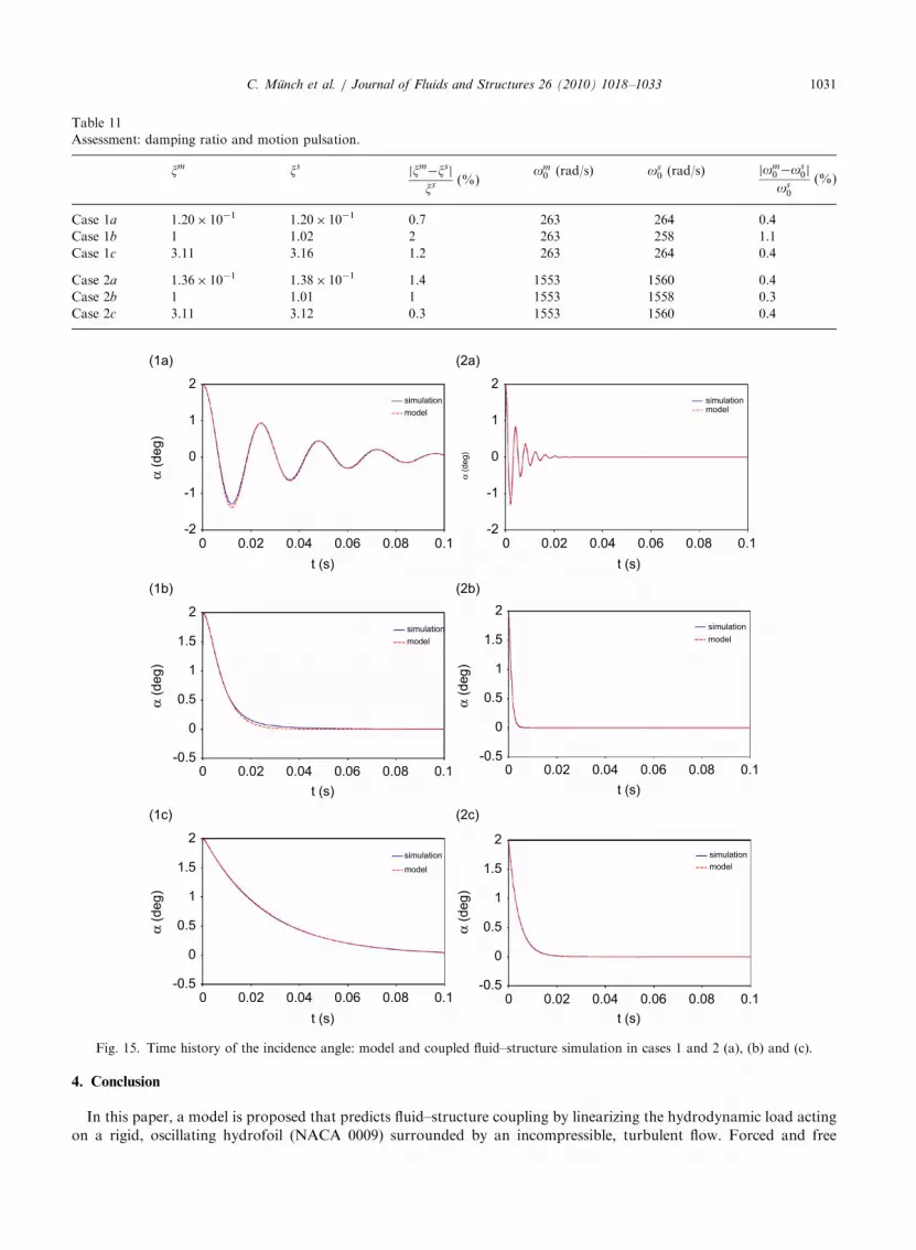
Fig. 15 shows the modeled and simulated time histories of the incidence angle plotted for the six cases. There is
excellent agreement between the coupled fluid–structure simulation, and the model is confirmed. Thus, it has been
shown that the forced motion simulation is sufficient to predict the fluid–structure coupling of the free motion case and
avoid coupled fluid–structure simulations, thereby saving a significant amount of time. This method was successfully
validated for a small motion amplitude with linear assumption for a maximum value of a0 ¼ 5�.
To identify all model parameters, eight numerical simulations (eight different reduced frequencies) must be
performed for the forced motion case. The corresponding required computational time was 2 h per simulation with 4
cores Intel Xeon Nehalem, 2.93GHz. Therefore, the total CPU time to entirely define the hydro-elastic behavior of the
oscillating hydrofoil is 16 h. For every single coupled fluid–structure simulation for the free motion case, a
computational time of 4 h per simulation is required using the same computational system.
Table 10
Assessment: added moment of inertia, fluid stiffness and damping coefficient.
k Jf (kgm2) kf (Nm) mf (kgm2 s�1)
Cases 1 2.62 2.45� 10�6 �0.14 3.82� 10�4
Cases 2 15.50 2.45� 10�6 0.026 2.59� 10�4
2simulationmodel
α (d
eg)
1
0
-1
-2
2
α (d
eg)
1
0
-1
-20 0.02 0.04 0.06 0.08 0.1
t (s)0 0.02 0.04 0.06 0.08 0.1
t (s)
simulationmodel
simulation
model
simulationmodel
2
1.5simulationmodel
1
0.5
0
-0.5
2
1.5
1
0.5
0
-0.5
simulationmodel
α (d
eg)
α (d
eg)
2
1.5
1
0.5
0
-0.5
2
1.5
1
0.5
0
-0.5
α (d
eg)
α (d
eg)
0 0.02 0.04 0.06 0.08 0.1t (s)
0 0.02 0.04 0.06 0.08 0.1t (s)
0 0.02 0.04 0.06 0.08 0.1t (s)
0 0.02 0.04 0.06 0.08 0.1t (s)
Fig. 15. Time history of the incidence angle: model and coupled fluid–structure simulation in cases 1 and 2 (a), (b) and (c).
Table 11
Assessment: damping ratio and motion pulsation.
xm xsjxm�xsj
xs (%)om
0 (rad/s) os0 (rad/s) jom
0 �os0j
os0
(%)
Case 1a 1.20� 10�1 1.20� 10�1 0.7 263 264 0.4
Case 1b 1 1.02 2 263 258 1.1
Case 1c 3.11 3.16 1.2 263 264 0.4
Case 2a 1.36� 10�1 1.38� 10�1 1.4 1553 1560 0.4
Case 2b 1 1.01 1 1553 1558 0.3
Case 2c 3.11 3.12 0.3 1553 1560 0.4
C. Munch et al. / Journal of Fluids and Structures 26 (2010) 1018–1033 1031
4. Conclusion
In this paper, a model is proposed that predicts fluid–structure coupling by linearizing the hydrodynamic load acting
on a rigid, oscillating hydrofoil (NACA 0009) surrounded by an incompressible, turbulent flow. Forced and free
C. Munch et al. / Journal of Fluids and Structures 26 (2010) 1018–10331032
pitching motions were both investigated with a mean incidence angle of 01 and a maximum angle amplitude of 21. The
unsteady simulations of the flow were performed in ANSYS CFX and validated experimentally. An analysis of the
hydrodynamic load was performed as a function of the reduced frequency, varying from 0.02 to 100, and the Reynolds
number, varying from 5� 105 to 1.5� 106. The hydrodynamic load was linearized by combining the added moment of
inertia, fluid damping and fluid stiffness effects. The added moment of inertia was found to be constant as expected
from the potential flow analysis. With respect to the fluid damping and the fluid stiffness coefficients, new results were
found. Both coefficients can be expressed as a function of the reduced frequency with an appropriate normalization.
When k � 4 and kZ12, quadratic and power laws were found, respectively, for k*, the dimensionless fluid stiffness
coefficient and m�, the dimensionless fluid damping coefficient. In between the two limits, a perturbation arises, and the
flow dynamic in the wake of the hydrofoil is changed when kC4:6. The two layers of vorticity found in the wake,
combine to form a discrete concentration of vorticity. Those vortices can lead to thrust generation, and the drag and the
hydrodynamic torque are modified. For a given value of the reduced frequency, the presented model can predict the
hydrodynamic torque on the hydrofoil.
To validate the method, a simulation was performed with the hydrofoil attached to a flexible structure. Six cases were
investigated, that varied the value of the structural damping and stiffness coefficients. Two values of the reduced
frequency were investigated to study cases with and without vortices in the wake. The time history of the incidence angle
was used for the validation. The incidence angle, aðtÞ, was first determined using the linearized model with the expected
analytical solution and then simulated as a coupled fluid–structure simulation in ANSYS CFX. An excellent agreement
was found, the differences in damping ratio and motion pulsation in the six cases were less than 2%. In conclusion, the
results show that the proposed model can predict fluid–structure coupling with good precision when the response of the
system is linearized. The method was successfully validated for a maximum value of 51 for the motion amplitude.
Acknowledgements
The investigation reported in this paper is part of the work carried out for the HYDRODYNA, Eureka Research
Project n 3246, whose partners are the following: ALSTOM Hydro, ANDRITZ Hydro, EPFL, VOITH Hydro and
UPC CDIF. The project is also financially supported by the Swiss Federal Commission for Technology and Innovation
(CTI) and Swisselectric Research. The authors are very grateful to the HYDRODYNA technical committee for its
involvement and constant support in the project. Finally the staff of the Laboratory for Hydraulic Machines should be
thanked for their support in the experimental and numerical work.
References
Abbott, I.H, Von Doenhoff, A.E., Albert, E., 1945. Summary of airfoil data. NACA Report, 824.
Ausoni, P., Farhat, M., Escaler, E., Egusquiza, E., Avellan, F., 2007. Cavitation influence on von karman vortex shedding and induced
hydrofoil vibrations. ASME Journal of Fluids Engineering 129, 966–973.
Avellan, F., Henry, P., Ryhming, I.L., 1987. A new high speed cavitation tunnel. ASME Winter Annual Meeting, Boston 57, 49–60.
Brennen, C.E., 1982. A review of added mass and fluid inertial forces, Naval Civil Engineering Laboratory.
Caron, J.F., 2000. Etude de l’influence des instationnarit�es des �ecoulements sur le d�eveloppement de la cavitation. Th�ese EPFL 2284.
Carstens, V., Kemme, R., Schmitt, S., 2003. Coupled simulation of flow-structure interaction in turbomachinery. Aerospace Science
and Technology 7, 298–306.
Conca, C., Osses, A., Planchard, J., 1997. Added mass and damping in fluid–structure interaction. Computer Methods in Applied
Mechanics and Engineering 146, 387–405.
Dowell, E.H., Hall, K.C., 2001. Modeling of fluid–structure interaction. Annual Review of Fluid Mechanics 33, 445–490.
Ducoin, A., Astofli, J.A., Deniset, F., Sigrist, J.F., 2009. An experimental and numerical study of the hydroelastic behavior of an
hydrofoil in transient pitching motion. In: First International Symposium on Marine Propulsors, Trondheim, Norway.
Gnesin, V.I., Kolodyazhnaya, L.V., Rzadkowski, R., 2004. A numerical modelling of stator–rotor interaction in a turbine stage with
oscillating blades. Journal of Fluids and Structures 19, 1141–1153.
Koochesfahani, M.M., 1989. Vortical patterns in the wake of an oscillating airfoil. AIAA Journal 27, 1200–1205.
Launder, B.E., Spalding, D.B., 1974. The numerical computation of turbulent flows. Computer Methods in Applied Mechanics and
Engineering 3 (2), 269–289.
Marshall, J.G., Imregun, M., 1996. A review of aeroelasticity methods with emphasis on turbomachinery applications. Journal of
Fluids and Structures 11, 973–982.
Menter, F.R., 1994. Two-equation eddy-viscosity turbulence models for engineering application. AIAA Journal 32 (8), 1598–1605.

C. Munch et al. / Journal of Fluids and Structures 26 (2010) 1018–1033 1033
Moffatt, S., He, L., 2005. On decoupled and fully-coupled methods for blade forced response prediction. Journal of Fluids and
Structures 20, 217–234.
Nicolet, C., Ruchonnet, N., Avellan, F., 2006. One-dimensional modeling of rotor stator interaction in Francis pumpturbine. In: 23rd
IAHR Symposium, Yokohama.
Triantafyllou, G.S., Triantafyllou, M.S., Grosenbaugh, M.A., 1993. Optimal thrust development in oscillating foils with application to
fish propulsion. Journal of Fluids and Structures 7, 205–224.
Wang, W.Q., He, X.Q., Zhang, L.X., Liew, K.M., Guo, Y., 2009. Strongly coupled simulation of fluid–structure interaction in a
francis hydroturbine. International Journal for Numerical Methods in Fluids 60, 515–538.
West, G.S., Apelt, C.J., 1982. The effects of tunnel blockage and aspect ratio on the mean flow past a circular cylinder with Reynolds
numbers between 104 and 105. Journal of Fluid Mechanics 114, 301–377.
Wilcox, D., 1993. Comparison of two-equation turbulence models for boundary layers with pressure gradient. AIAA Journal 31 (8),
1414–1421.
Young, Y.L., 2007. Time-dependant hydroelastic analysis of cavitating propulsors. Journal of Fluids and Structures 23, 269–295.
Young, Y.L., 2008. Fluid–structure interaction analysis of flexible composite marine propellers. Journal of Fluids and Structures 24,
799–818.
Zobeiri, A., Kueny, J.L., Fahrat, M., Avellan, F., 2006. Pump-turbine rotor–stator interactions in generating mode: pressure
fluctuation in distributor channel. In: 23rd IAHR Symposium, Yokohama, Japan.
Recommended


