Download pdf - investigating the effect of column orientations on - METU

INVESTIGATING THE EFFECT OF COLUMN ORIENTATIONS ON MINIMUM WEIGHT DESIGN OF STEEL FRAMES

A THESIS SUBMITTED TO THE GRADUATE SCHOOL OF NATURAL AND APPLIED SCIENCES

OF MIDDLE EAST TECHNICAL UNIVERSITY

BY

MELĐSA KIZILKAN

IN PARTIAL FULFILLMENT OF THE REQUIREMENTS FOR

THE DEGREE OF MASTER OF SCIENCE IN

CIVIL ENGINEERING

JANUARY 2010

Approval of the thesis:

INVESTIGATING THE EFFECT OF COLUMN ORIENTATIONS ON

MINIMUM WEIGHT DESIGN OF STEEL FRAMES

submitted by MELĐSA KIZILKAN in partial fulfillment of the requirements for the degree of Master of Science in Civil Engineering Department, Middle East Technical University by,

Prof. Dr Canan Özgen Dean, Graduate School of Natural and Applied Sciences

Prof. Dr. Güney Özcebe

Head of Department, Civil Engineering Assoc. Prof. Dr Oğuzhan Hasançebi Supervisor, Civil Engineering Dept., METU Examining Committee Members: Prof. Dr Mehmet Polat Saka Engineering Science Dept., METU

Assoc. Prof. Dr Oğuzhan Hasançebi Civil Engineering Dept., METU Assist. Prof. Dr Özgür Kurç Civil Engineering Dept., METU Assist. Prof. Dr Ayşegül Askan Gündoğan Civil Engineering Dept., METU

Assist. Prof. Dr Afşin Sarıtaş Civil Engineering Dept., METU Date:

iii

I hereby declare that all information in this document has been obtained and presented in accordance with academic rules and ethical conduct. I also declare that, as required by these rules and conduct, I have fully cited and referenced all material and results that are not original to this work.

Name, Last name: Melisa Kızılkan Signature :

iv

ABSTRACT

INVESTIGATING THE EFFECT OF COLUMN ORIENTATIONS ON MINIMUM WEIGHT DESIGN OF STEEL FRAMES

Kızılkan, Melisa

M.S., Department of Civil Engineering

Supervisor: Assoc. Prof. Dr. Oğuzhan Hasançebi

January 2010, 146 pages

Steel has become widespread and now it can be accepted as the candidate of

being main material for the structural systems with its excellent properties. Its

high quality, durability, stability, low maintenance costs and opportunity of fast

construction are the advantages of steel. The correct use of the material is

important for steel’s bright prospects. The need for weight optimization

becomes important at this point. Available sources are used economically

through optimization. Optimization brings material savings and at last

economy. Optimization can be achieved with different ways. This thesis

investigates the effect of the appropriate choice of column orientation on

minimum weight design of steel frames. Evolution strategies (ESs) method,

which is one of the three mainstreams of evolutionary algorithms, is used as the

optimizer in this study to deal with the current problem of interest. A new

evolution strategy (ES) algorithm is proposed, where design variables are

considered simultaneously as cross-sectional dimensions (size variables) and

orientation of column members (orientation variables). The resulting algorithm

is computerized in a design optimization software called OFES. This software

has many capabilities addressing to issues encountered in practical

applications, such as producing designs according to TS-648 and ASD-AISC

design provisions. The effect of column orientations is numerically studied

v

using six examples with practical design considerations. In these examples,

first steel structures are sized for minimum weight considering the size

variables only, where orientations of the column members are initially assigned

and kept constant during optimization process. Next, the weight optimum

design of structures are implemented using both size and orientation design

variables. It is shown that the inclusion of column orientations produces

designs which are generally 4 to 8 % lesser in weight than the cases where only

size variables are employed.

Keywords: Optimization, Structural optimization, Evolution algorithms,

Evolution strategies, Structural design, Steel frames, Optimal choice of column

orientations.

vi

ÖZ

KOLON DOĞRULTULARI SEÇĐMĐNĐN MĐNĐMUM AĞIRLIKLI ÇELĐK ÇERÇEVE YAPI TASARIMINA ETKĐSĐNĐN ĐNCELENMESĐ

Kızılkan, Melisa

Yüksek Lisans, Đnşaat Mühendisliği Bölümü

Tez Yöneticisi: Doç. Dr. Oğuzhan Hasançebi

Ocak 2010, 146 sayfa Mükemmel özellikleri ile yapısal sistemlerin birinci öncelikli malzemesi

olmaya aday olan çelik giderek yaygınlaşmaktadır. Çeliğin yüksek kalitesi,

dayanıklılığı, stabilitesi, düşük bakım masrafları ve hızlı inşası avantajlı

yönleridir. Malzemenin doğru kullanımı çeliğin parlak geleceği için önemlidir.

Ağırlık optimizasyonu bu noktada önem kazanmaktadır. Mevcut kaynaklar

optimizasyonun devreye girmesi ile en ekonomik şekilde kullanılmaktadır.

Optimizasyon malzeme tasarrufunu ve ekonomiyi sağlamaktadır.

Optimizasyon farklı yollarla gerçekleştirilebilir. Bu tez, kolonlarda uygun

doğrultu seçiminin minimum ağırlıklı çelik yapı tasarımına etkisini

incelemektedir. Evrimsel algoritmanın üç ana dalından biri olan evrimsel

stratejiler (ESs) metodu bu çalışmadaki problemlerin çözümünde optimizasyon

aracı olarak kullanılmıştır. Tasarım değişkeni olarak aynı anda kesit alan

boyutlarını (boyut değişkeni) ve kolon elemanlarının doğrultularını (doğrultu

değişkeni) dikkate alan yeni bir evrimsel strateji (ES) algoritması ileri

sürülmüştür. Ortaya çıkan algoritma, tasarım optimizasyonunun yapıldığı

yazılım programı OFES’te kullanılmıştır. Bu program, pratikte yer alan

uygulamalarda TS–648 ve ASD-AISC standartlarına göre çözümler

üretebilmektedir. Kolon oryantasyonunun etkisi, altı örnekle pratik tasarım

esasları doğrultusunda sayısal olarak çalışılmıştır. Bu örneklerde ilk olarak,

vii

kolon doğrultuları önceden belirlenmiş ve sabit olarak bırakılmış çelik yapılar,

sadece boyut değişkenleri dikkate alınarak boyutlandırılmıştır. Daha sonra, bu

yapıların optimum ağırlık tasarımları hem boyut hem de doğrultu tasarım

değişkenlerinin kullanılmasıyla gerçekleştirilmiştir. Kolon doğrultularının

tasarım değişkenlerine eklenmesi, sadece boyut değişkenlerinin kullanıldığı

durumlara oranla genellikle % 4 ile 8 arasında daha hafif tasarımlar elde

edilmesini sağlamaktadır.

Anahtar Kelimeler: Optimizasyon, Yapı optimizasyonu, Evrimsel algoritmalar,

Evrimsel stratejiler, Yapı tasarımı, Çelik çerçeveler, Kolon doğrultularının en

uygun seçimi.

viii

To My Parents and Grandmother,

ix

ACKNOWLEDGMENTS

The author wishes to express her deepest gratitude to her supervisor Assoc.

Prof. Dr. Oğuzhan Hasançebi for his guidance, careful supervision, criticisms,

patience and insight throughout the research.

I’m grateful to my mother Beyhan Kızılkan and my father Veli Kızılkan for

giving their love, patience and support during my endless school life and it was

my chance that each time despair knocks the door they was there to give their

helping hand. It is beyond description for the author to express her intense

feelings to her parents and she is praying for a lifetime support of them.

I would embrace my grandmother Hadiye Eper with pure love and respect for

her warm and compassionate receiving with open arms; she was the one who

entertains a kindly feeling for me.

I should mention that it would be a proud of mine to try to pay my gratitude to

my aunt, my uncle, my cousins, my aunt in law and my uncle in law, who is far

away from us, and to Đzmir and to all the ones who lives in Đzmir.

I would have been incomplete, if I didn’t have my dearest friends with whom

life blossoms and is a pleasure to see them after awakening from the ever

darkest nights.

The author presents her respects to PROKON Engineering and to her

colleagues who have great helps and supports to her, while she was both

studying and working. It was my chance to walk with them all through the

same way.

x

My endless thanks are for my school and solution partners, they were always

there with their cheerful personalities all through my limited time in school,

and the author is seeking for a lifetime friendship.

xi

TABLE OF CONTENTS

ABSTRACT ...................................................................................................... iv

ÖZ...................................................................................................................... vi

ACKNOWLEDGMENTS................................................................................. ix

TABLE OF CONTENTS .................................................................................. xi

LIST OF TABLES .......................................................................................... xiv

LIST OF FIGURES......................................................................................... xvi

LIST OF SYMBOLS....................................................................................... xix

LIST OF SYMBOLS....................................................................................... xix

CHAPTERS

1. INTRODUCTION.......................................................................................... 1

1.1 OBJECTIVES....................................................................................... 2

1.2 SCOPE.................................................................................................. 3

2. LITERATURE SURVEY / BACKGROUND ............................................... 6

2.1 REVIEW OF THE LITERATURE...................................................... 6

3. EVOLUTION STRATEGY METHOD....................................................... 10

3.1 SEARCH TECHNIQUES .................................................................. 10

3.2 GLOBAL OPTIMIZATION .............................................................. 12

3.3 EVOLUTION STRATEGIES ............................................................ 15

3.4 EVOLUTION STRATEGIES WITH CONTINUOUS DESIGN

VARIABLES.................................................................................................. 16

3.4.1 Basic Concepts in Evolution Strategies...................................... 18

3.5 EVOLUTION STRATEGIES WITH DISCRETE DESIGN

VARIABLES.................................................................................................. 27

xii

3.5.1 Discrete Mutation ....................................................................... 28

3.5.2 The Approach Proposed by Bäck and Schütz ............................ 29

3.5.3 The Approach Proposed by Cai and Thierauf ............................ 31

3.5.4 The Approach Proposed by Rudolph ......................................... 32

3.5.5 A Reformulation of Rudolph’s Approach .................................. 34

4. MINIMUM WEIGHT DESIGN PROBLEM FORMULATION OF STEEL

FRAMES.......................................................................................................... 37

4.1 DESIGN VARIABLES AND OBJECTIVE FUNCTION................. 37

4.2 AXIAL AND BENDING STRESS CONSTRAINTS ....................... 38

4.3 SHEAR STRESS CONSTRAINTS ................................................... 41

4.4 SLENDERNESS CONSTRAINTS.................................................... 42

4.5 DISPLACEMENT AND DRIFT CONSTRAINTS........................... 42

4.6 GEOMETRIC CONSTRAINTS ........................................................ 42

5. OPTIMIZATION ALGORITHM AND SOFTWARE ................................ 44

5.1 A GENERAL FLOWCHART............................................................ 44

5.2 DETAILED ALGORITHM ............................................................... 46

5.2.1 Initial Population ........................................................................ 46

5.2.2 Evaluation of Population ............................................................ 47

5.2.3 Recombination............................................................................ 48

5.2.4 Mutation ..................................................................................... 49

5.2.5 Selection ..................................................................................... 52

5.2.6 Termination ................................................................................ 52

5.3 “OFES” SOFTWARE ........................................................................ 52

5.3.1 The Use of Software................................................................... 52

5.3.2 Practical Features of Ofes........................................................... 57

6. DESIGN EXAMPLES ................................................................................. 59

6.1 INTRODUCTION.............................................................................. 59

6.2 DESIGN LOADS ............................................................................... 60

6.2.1 Gravity Loads ............................................................................. 61

6.2.2 Lateral Wind Loads .................................................................... 62

xiii

6.3 PROFILE LIST AND MATERIAL PROPERTIES........................... 64

6.4 ES PARAMETERS............................................................................ 64

6.5 DESIGN EXAMPLE 1: 960 MEMBER STEEL FRAME ................ 64

6.5.1 Structural System ....................................................................... 65

6.5.2 Test Results ................................................................................ 72

6.6 DESIGN EXAMPLE 2: 568 MEMBER STEEL FRAME ................ 89

6.6.1 Structural System ....................................................................... 89

6.6.2 Test Results ................................................................................ 97

6.7 DESIGN EXAMPLE 3: 1230 MEMBER STEEL FRAME ............ 105

6.7.1 Structural System ..................................................................... 105

6.7.2 Test Results .............................................................................. 113

6.8 DESIGN EXAMPLE 4: 3590 MEMBER STEEL FRAME ............ 117

6.8.1 Structural System ..................................................................... 117

6.8.2 Test Results .............................................................................. 129

6.9 RESULTS AND EVALUATION .................................................... 137

7. CONCLUSION .......................................................................................... 141

7.1 CONCLUSIONS AND SUGGESTIONS ........................................ 141

7.2 RECOMMANDATIONS FOR FUTURE STUDIES ...................... 142

REFERENCES............................................................................................... 143

xiv

LIST OF TABLES

TABLES Table 6-1 General properties of design examples ............................................ 60

Table 6-2 Load Combinations.......................................................................... 61

Table 6-3 Member grouping for 960 member steel frame. .............................. 70

Table 6-4 Gravity loading on the beams of 960 member steel frame. ............ 72

Table 6-5 Wind Loading Values under Wind Speeds of 90mph and 105mph (in

kN/m, lb/ft)................................................................................................ 72

Table 6-6 Wind Loading Values under Wind Speeds of 120mph and 150mph

(in kN/m, lb/ft) .......................................................................................... 73

Table 6-7 The minimum design weights and volumes obtained for 960-member

frame in eight runs for the basic wind speed case of 90=V mph............ 75

Table 6-8 A comparison of best designs obtained for 960-member steel frame

for the basic speed wind case of 90=V mph. ........................................ 76


frame in eight runs for the basic wind speed case of 105=V mph ........ 79


for the basic speed wind case of 105=V mph........................................ 80

Table 6-11 The minimum design weights and volumes obtained for 960-

member frame in eight runs for the basic wind speed case of 120=V mph

................................................................................................................... 84


for the basic speed wind case of 120=V mph........................................ 84



................................................................................................................... 87


for the basic speed wind case of 150=V mph. ........................................ 88

xv

Table 6-15 Member grouping for 568 member steel frame ............................ 92

Table 6-16 Gravity loading on the beams of 568 member steel frame .......... 97

Table 6-17 Wind Loading Values under Wind Speed of 105mph(in kN/m,lb/ft).

................................................................................................................... 97

Table 6-18 Torsional Moment Values (in kNm, lbft). ..................................... 97


member frame in eight runs. ..................................................................... 99

Table 6-20 A comparison of best designs obtained for 568-member steel frame.

................................................................................................................. 100


member frame in eight runs. ................................................................... 103


................................................................................................................. 104

Table 6-23 Member grouping for 1230 member steel frame. ........................ 111

Table 6-24 Gravity loading on the beams of 1230 member steel frame. ...... 113

Table 6-25 Wind Loading Values under Wind Speed of 105mph (in kN/m,lb/ft).

................................................................................................................. 113



Table 6-27 A comparison of best designs obtained for 1230-member steel

frame. ...................................................................................................... 115

Table 6-28 Member grouping for 3590-member steel frame......................... 124

Table 6-29 Gravity loading on the beams of 3590 member steel frame. ...... 128

Table 6-30 Wind Loading Values under Wind Speed of 105mph (in

kN/m,lb/ft)............................................................................................... 129




frame. ...................................................................................................... 131

xvi

LIST OF FIGURES

FIGURES Figure 3.1 Categorization of search techniques ............................................... 10

Figure 3.2 Mutation with n=2, nσ=1, nα=0 [30] ............................................... 22

Figure 3.3 Mutation with n=2, nσ=2, nα=0 [30] .............................................. 24

Figure 3.4 Mutation with n=2, nσ=2, nα=1 [30] ............................................... 25

Figure 3.5 Poisson distribution for some selected values of c. ........................ 32

Figure 3.6 Geometric distribution for some selected values of ψ ................... 33

Figure 4.1 Element local coordinate system .................................................... 38

Figure 4.2 Beam-column geometric constraints............................................... 44

Figure 5.1 General flowchart of the ES algorithm developed in the study. .... 47

Figure 5.2 Opening screen of OFES ................................................................ 57

Figure 5.3 The generation of geometric model internally using SAP2000 v7.4

from OFES. ............................................................................................... 58

Figure 5.4. “OFES-3D Define Data” window.................................................. 58

Figure 5.5“OFES-3D Define Constraint” window........................................... 59

Figure 5.6“OFES-3D Project Output” window................................................ 59

Figure 5.7 Extruded view of the best design. ................................................... 60

Figure 6.1 Design wind load cases [43] ........................................................... 64

Figure 6.2 960 member steel frame................................................................. 71

Figure 6.3 Grouping of members of 960-member steel frame in plan level. ... 72

Figure 6.4 Design history graph for the basic speed wind case of 90=V mph.

................................................................................................................... 77

Figure 6.5 Optimal layout column orientation for 960-member steel frame for

the basic speed wind case of 90=V mph............................................... 80


................................................................................................................... 81

xvii


the basic speed wind cases of 105=V and 120 mph. .............................. 84


................................................................................................................... 85


................................................................................................................... 89


the basic speed wind cases of 150=V mph.............................................. 92

Figure 6.11 568 member steel frame............................................................... 97

Figure 6.12 Grouping of members of 568-member steel frame in plan level .. 98

Figure 6.13 Design history graph of 568 member steel frame....................... 101

Figure 6.14 Optimal layout column orientations for 568-member steel frame.

................................................................................................................. 104

Figure 6.15 Design history graph of 568 member steel frame....................... 105


................................................................................................................. 108

Figure 6.17 1230-member steel frame .......................................................... 112

Figure 6.18 Vertical bracings and moment releases of 1230 member steel frame

................................................................................................................. 112

Figure 6.19 Grouping of members of 1230-member steel frame in plan view

................................................................................................................. 113

Figure 6.20 Design history graph of 1230 member steel frame..................... 119

Figure 6.21 Optimal layout column orientation for 1230-member steel frame.

................................................................................................................. 120

Figure 6.22 3590 member steel frame........................................................... 124

Figure 6.23 Grouping of members of 3590-member steel frame in plan level.

................................................................................................................. 125

Figure 6.24 Design history graph of 3590 member steel frame..................... 138


................................................................................................................. 139

Figure 6.26 Lateral loading of a general steel frame...................................... 143

xviii

Figure 6.27 Behavior of a frame under lateral loading .................................. 144

xix

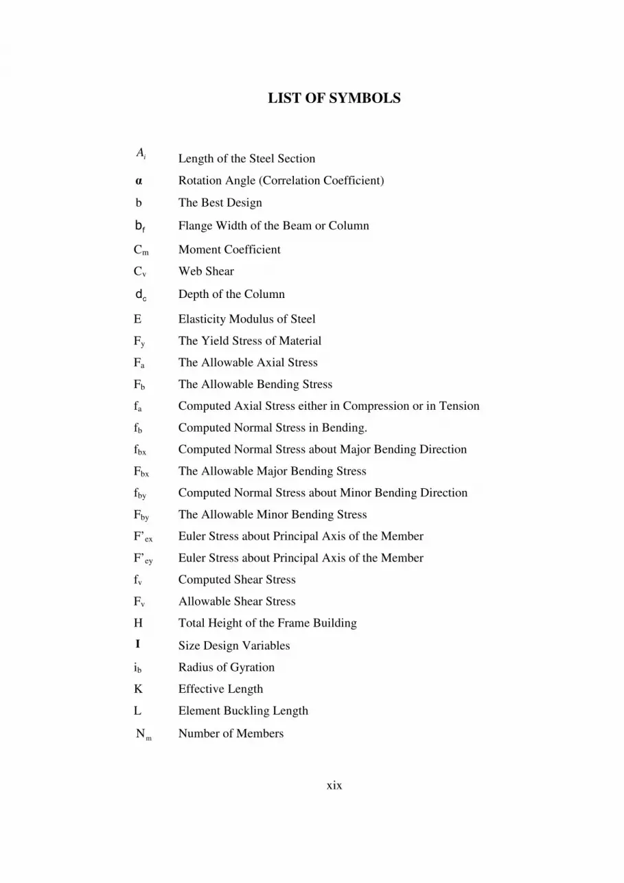
LIST OF SYMBOLS

iA Length of the Steel Section

α Rotation Angle (Correlation Coefficient)

b The Best Design

fb Flange Width of the Beam or Column

Cm Moment Coefficient

Cv Web Shear cd Depth of the Column

E Elasticity Modulus of Steel

Fy The Yield Stress of Material

Fa The Allowable Axial Stress

Fb The Allowable Bending Stress

fa Computed Axial Stress either in Compression or in Tension

fb Computed Normal Stress in Bending.

fbx Computed Normal Stress about Major Bending Direction

Fbx The Allowable Major Bending Stress

fby Computed Normal Stress about Minor Bending Direction

Fby The Allowable Minor Bending Stress

F’ex Euler Stress about Principal Axis of the Member

F’ey Euler Stress about Principal Axis of the Member

fv Computed Shear Stress

Fv Allowable Shear Stress

H Total Height of the Frame Building

I Size Design Variables

ib Radius of Gyration

K Effective Length

L Element Buckling Length

mN Number of Members

xx

dN Sizing Groups

oN Number of Orientation Groups for Column Members

O Orientation Design Variables

ps Relative Frequency

P(0) Initial Population

1)P(t + Parent Population of the Next Generation

p Mutation Probability

r Minimum Radius of Gyration

sb Unbraced Member Lengths

)s(φ Adaptive Strategy Parameters

s Arbitrary Component of an Individual

ft Flange Width of the Column

x Design Variable Vector

W Weight of the Frame

z N-dimensional Random Vector.

α Penalty Coefficient

µ Parent

λ Offspring

σ Standard Deviation

ξ Mean

iκ Distributed Integer Random Number

iρ Unit Weight of the Steel Section

ψ Set of Geometric Distribution Parameters

φ Constrained Objective Function Value

γ Learning Rate

τ Learning Rate

1

CHAPTER 1

INTRODUCTION

Developments in computer technology, advances in material quality and the

idea of seeking for the best solution accelerated the studies on economical

structural systems that can be analyzed in short durations. In the last decade

developments in architecture and increasing demands for high rise buildings

resulted in systematic design of steel structures.

Steel plays an important role in this development process. It not only exhibits

certain advantages over other materials in terms of its mechanical

characteristics, such as high strength and ductility, but also offers an

opportunity for assembling different structural frame systems for massive parts.

The idea of using steel is also related with gravity loads. As the building

becomes higher the columns from top to bottom are subjected to greater loads.

Steel yields both aesthetic and economical solutions to such structures. It is

possible to use different sections of columns from bottom to top without

compromising aesthetics.

It is important to use optimization techniques in steel, whose superior material

properties are implied. A structural system that is not only strong enough to

satisfy the limitations but also light enough to minimize the usage of natural

sources can be satisfied with the correct choice of members. A light weighted

structure will be in benefit of environmental factors and also will help the

minimization of the earthquake forces. Slender members that satisfy the

limitations will help the aesthetic concerns.

2

Mathematical programming techniques and optimality criteria have long been

used in structural optimization problems. The design variables were assumed to

be continuous in these derivation-based methods. At the end of the

optimization, the results were chosen from continuous design sets. Usually the

results were not relevant to the practical fabrication requirements.

The studies continued to overcome these drawbacks of the existing methods,

and accordingly new techniques have emerged. Metaheuristic search

algorithms, which use nature as a source of inspiration to develop numerical

solution algorithms, have five branches. Simulated annealing, evolutionary

algorithms, tabu search, harmony search, swarm-based optimization are the

techniques that belong to the metaheuristic search algorithms. These algorithms

do not require any gradient information of the objective function and

constraints and the transition rules are not deterministic any more, instead

probabilistic transition rules are used [1]. There is another attractive feature of

metaheuristic search algorithms. In addition to continuous variables, these

methods can also deal with discrete design variables, which in fact give an

opportunity to the designer to select members from a list of ready sections.

1.1 OBJECTIVES

Columns and beams are the main members of steel structures. The relevant

orientation of the elements plays an important role in the weight of the system.

Each of the member groups should be placed in right position so that their

strong axis can resist on the exerted forces. When designing space steel

structures, beams are placed such that the major bending axis coincides with

the strong axis of the beam, whereas columns are oriented in any direction

depending on the intuition of the designer.

The column orientations can be predicted according to some design heuristics.

If the plan of the structure is square or almost square the system needs to have

3

the same rigidity in both directions. This can be satisfied with column

orientations. The number of columns whose strong axes are in the same

direction with x axis of the structure should be equal to the one’s that are in y

direction. By this way the building’s resistance to the lateral loads will be

similar in both directions. In case of a rectangular building, columns are placed

with their strong axis perpendicular to short side in order to increase resistance

of the building against bending along short side.

The optimum design process of the steel frames in the literature is only based

on sizing of structural members in which orientations of the columns are

determined initially and kept constant during optimum design process. The

objective of the thesis is to investigate the effect of the choice of column

orientation on minimum weight design of steel frames. Evolution strategy

method, which is one of the three mainstreams of Evolutionary Algorithms, is

used as the optimizer in the study to deal with the current problem of interest.

In the study, a new ES algorithm is proposed, where design variables are

considered simultaneously as cross-sectional dimensions (size variables) and

orientation of column members (orientation variables.)

1.2 SCOPE

The rest of the thesis is organized as follows:

In Chapter 2, literature survey is carried out. Preceding studies on the use of

evolution strategies technique in structural optimization applications are briefly

summarized. It is emphasized that the literature lacks studies where orientation

of the columns are used as design variables in the optimum design process of

steel frames.

In Chapter 3, evolution strategies (ESs) method is introduced thoroughly. The

development of the method and its enhancements over time are mentioned. It is

4

noted that the method was originally developed as a continuous variable

optimization technique, and later it was reformulated in the literature to deal

with discrete variables also. Although not used effectively in the thesis,

continuous ESs and their variants are overviewed first to describe the

fundamentals of the technique. Next, various reformulations of discrete ESs

proposed in the literature are overviewed.

In Chapter 4, the problem formulation regarding the weight optimum design of

space steel structures are presented. In this chapter, the stress, stability and

displacement imposed according to Allowable Stress Design- American

Institute of Civil Engineers (ASD-AISC) are formulated. In addition, geometric

constraints that imposed considering practical requirements of the design

process are also formulated.

Chapter 5 describes about the ES algorithm developed for optimum design of

steel frames where size and optimization variables are implemented

simultaneously to minimize the structural weight of such systems. The

resulting is computerized in a software called OFES. The capabilities and

practical features of the software are also discussed here.

Numerical examples are presented in Chapter 6. Six design examples are

studied in all to scrutinize the effect of column orientation on minimum weight

design of steel structures. For each design example, full design data including

loadings, element definitions and member groupings is provided. Each

example is first designed for minimum weight considering size variables only,

where orientations of the columns are assigned initially and kept unvarying

during the optimum design process. Next, the example is reworked in which a

minimum weight design is sought for the same system by taking both size and

orientation variables as the design variables in the process. Optimum designs

are reported in each case in terms of the discrete sections attained for member

groups and orientations of the column members in optimum design model. A

5

comparison is carried out between these cases to quantify the effect of the

choice of column orientation.

Finally Chapter 7 concludes the thesis and summarizes some important results

of the study.

6

CHAPTER 2

LITERATURE SURVEY / BACKGROUND

2.1 REVIEW OF THE LITERATURE

Metaheuristic techniques imitate the paradigm of natural evolution observed in

biological organism to improve a set of designs using the evolutionary

principles. Evolutionary algorithms belong to the group of metaheuristic

techniques in which evolution strategies is placed. Evolution strategy is

employed as the tool for optimization in this study. In the following, major

studies in the literature that employ ESs method in structural optimization

applications are briefly overviewed.

Papadrakakis et al. [2] studied structural optimization using evolution

strategies and neural networks. It is mentioned that a gradient based

optimization has the drawback of performing a great deal of sensitivity

analysis. On the other hand evolution strategies do not require any sensitivity

analysis. They have an advantage of robustness and better global behavior and

disadvantage of the method is slow rate of convergence towards the global

optimum. In the light of previous studies on artificial neural networks (ANN)

the use of ANN in ESs in sizing and shape problems is investigated and

drawbacks of ESs method are tried to be eliminated. Structural problems are

solved in the scope of the study to see the advantages of the new combinatory

method. The selection of the training set is also investigated. Randomly chosen

combinations of input data using a Gaussian distribution around the midpoints

of the design space is accepted as the best training set selection scheme. The

study concluded that, combination of ANN and ES is quite useful and

advantageous for optimization. The time consuming parts of optimization

process are handled in relatively short time intervals.

7

Multi objective discrete optimization of laminated structures was performed by

Spallino and Rizzo [3]. A multi-objective design problem refers to a case where

more than one objective function is defined. Spallino and Rizzo started to work

in line with the work of Pareto [4] who has studied multi objective

optimization first. In the study, multi-objective design problem for laminated

composite structures is carried out using two different examples. A rectangular

laminated plate is studied with design objectives of critical buckling load,

critical temperature rise and failure load maximization. A laminated cantilever

plate is the second problem of the study where the minimization of tip

displacement and rotation and the minimization of the first natural frequency

are taken as the design objectives. The problems have different loading and

layouts but both have discrete design variables. The problems are solved with a

method that is based on ES and game theory (bargaining method). The study

came up with a result that the combination of ES with game theory is useful for

the multi objective optimization [3].

Gutkowski, Iwanow and Bauer [5] concentrated on design of structural systems

with minimum weight. The idea behind their study is to design the structure

with controlled mutation. In this application, mutations are controlled by

stresses whereas they are controlled by state variables in the others. Largest

and smallest stresses are randomly verified in the optimized problems for the

control step of the algorithm [5]. The study concluded that this method marks

out for a brilliant future and studies can be continued for this method.

Lagaros et al. [6] is concerned with the improvement of the performance of the

optimization procedure by modifying evolutionary algorithm. They discuss that

genetic algorithms and evolution strategies have several advantages compared

to other approaches. However, the major drawback of these approaches lies in

their time consuming processes. Mathematical programming method is

integrated to both genetic algorithms and evolution strategies for the purpose of

forming hybrid methodologies to eliminate the aforementioned drawbacks of

8

these techniques. Sequential quadratic programming (SQP), which is regarded

as the most robust mathematical programming method, is included to the

algorithm to increase the efficiency of these techniques. Numerical examples

are performed to evince the efficiency gained with the hybrid methods.

Ebenau et al [7] developed an advanced evolution strategy algorithm with an

adaptive penalty function for mixed-discrete structural optimization. In this

work it is clearly stated that a small reduction of weight may also lead to a

considerable decrease of the costs of manufacturing, transport and assembly. It

is also stated that low weight of profiles means that slender members are in use

and this brings about the problem of buckling. The need of a program that

investigates not only buckling problems but also stability effects is exposed. In

this study, these issues are taken care of by adding an adaptive penalty function

to the (µ+1)-evolution strategy. The numerical effort is reduced with the help

of (µ+1)-evolution strategy in the study. A mutation procedure was added to

the computational steps which gives the algorithm an opportunity to reach the

global optimum. The study is concluded that most convenient penalty function

is the one which depends on both the constraint value and actual rate of

feasible individuals in the current population. It is noted that optimization with

mixed-discrete variables can be solved with the variant of (µ+1)-evolution

strategy. The adaptation to the strategy is the utilized mutation operator and the

combination with a penalty function that works robust and efficient [7].

In Lagaros et al. [8] the performance improvement of the evolution strategies

in the structural optimization is addressed. This improvement is investigated in

conjunction with especially large scale structures. In the study neural network

(NN) strategy is used to replace computationally expensive finite element

analyses required by ESs with inexpensive and acceptable approximation of the

exact analysis. The algorithms are implemented on two computing platforms;

sequential and parallel computing environments. Different adaptive NN

training schemes are examined to find the best performance. Both large and

9

small starting training sets are chosen. It is observed that small initial training

sets are better than the large ones from performance standpoint. The idea

behind the strategy of adaptively creating the NN training set is providing an

NN configuration gradually with prediction capabilities for the regions of the

overall design space that are actually visited by the ES procedure [8].

In study of Rajasekaran et al. [9] space structures are optimized for minimum

weight with functional networks. It is stated that classical optimization

methods are not appropriate for large scale structures, because of time

consuming sensitivity analysis. On the other hand, probabilistic search

methods, (such as ESs), are not gradient based methods so that no sensitivity

analysis is required for their implementation. Formex algebra of the Formian

software [10] is chosen to generate the geometry of large scale space structure.

Encouraging results are obtained for several design examples considered in the

study and it is concluded that the method proposed is a very efficient method.

In another study by Baumann and Kost [11] [10] , topology optimization of

discrete structures such as trusses is studied with ESs technique. It is stated that

the most common approach for topology optimization is ground structure

method. With this method, unnecessary elements of highly connected initial

structures are eliminated until the objective function is reached.

10

CHAPTER 3

EVOLUTION STRATEGY METHOD

3.1 SEARCH TECHNIQUES

As shown in Figure 3.1 search techniques of optimization techniques can

coarsely be classified into three main groups as enumerative techniques,

calculus based techniques and global optimization techniques.

Figure 3.1 Categorization of search techniques

Enumarative techniques, in principle, search every possible point in design

space or domain one point at a time. They can be simple to implement but the

number of possible points may be too large for direct search. Calculus based

techniques use the gradient values to estimate the location of nearby optimum.

These techniques are known as Hill Climbing techniques because they estimate

11

where the maximum lies, move to that point, make a new estimate, and make a

new move and repeat this process until they reach the top of the hill.

Global optimization techniques have received increased attention, primarily

because of their lack of dependence on gradient information, a more robust

approach to handle discrete and integer design variables, and for an enhanced

ability to locate the globally optimal solution; particularly in discrete

optimization problems.

In the past, conventional optimization techniques (optimality criteria and

mathematical programming methods) overwhelmingly controlled the early

applications in the area of structural optimization. The majority of conventional

techniques work on the basis of derivation of objective function and constraints

with respect to design variables, that is to say, they accomplish a gradient-

based search. However, this situation highly hampers their applicability to

complex structural optimization problems. There are several reasons for this.

Firstly, for a proper implementation of the gradient-based search, they

necessarily require a continuous design space, where the design variables can

assume any value between the specified bounds. Secondly, even if the

requirement for continuity of the design space is satisfied, the gradient-based

search followed by these techniques guides the process towards a point which

is usually the local optimum closest to the starting solution. Considering that

the design space incorporates many local optima, it is a very difficult task to

reach the global optimum, avoiding all those local optima. Accordingly, their

success is intimately dependent on the choice of a good starting solution, which

is in most cases unknown at the start. Finally, they are not well suited to

discrete variable optimization, where the design variables are to be selected

from an already available list, rather that being continuous, e.g., integer and 0-1

optimizations can easily be interpreted as two special cases of the general

discrete variable optimization approach. In particular, in civil engineering

structures; steel structures representing a very large and important group in this

12

respect, one has to choose the structural members from commercially available

profiles in the markets, and the number of bolts used for connections match an

integer number, etc. A customary approach followed by conventional

techniques to handle a discrete variable problem is first to solve the problem

using continuous variables, and then to round up the solution to the nearest

existing discrete values. But, this approach may easily lead to non-optimum or

infeasible solutions. Therefore, a computationally complex problem of this

nature calls for an efficient and reliable optimization method.

Recently, a number of global optimization techniques have emerged to be

promising strategies, showing certain superiorities over conventional

techniques in these aspects, together with their potential applicability for a

wide range of diverse problem areas. The underlying concepts of these

techniques and thus their algorithmic models have been constituted by

establishing correspondences between the optimization task and events

occurring in nature, i.e., nature is used as a source of inspiration. This feature

in turn brings about a solution methodology which completely rejects a

gradient-based search so as to reduce the possibility of getting stuck in a local

optimum. The most popular techniques in this category are evolutionary

algorithms (EAs), simulated annealing (SA), tabu search, harmony search, and

swarm-based optimization techniques as depicted in Figure 3.1.

3.2 GLOBAL OPTIMIZATION

Evolutionary algorithms refer to a group of techniques, which imitate the

paradigm of natural evolution observed in biological organism to improve a set

of designs using the evolutionary principles. Genetic algorithms, evolution

strategies and evolutionary programming are regarded as the three mainstreams

of evolutionary algorithms. Genetic algorithms were first introduced by

Holland [12]; early studies in evolution strategies were pioneered by

Rechenberg [13], [14] and Schwefel [15]; and evolutionary programming was

13

first put forward by Fogel [16]. The procedure used in any evolutionary

algorithm technique requires a stochastic and iterative process, which

endeavors to improve a population of designs (individuals) over a selected

number of generations.

The optimization task in the simulated annealing (SA) is achieved by following

another heuristic concept extending to the annealing process of physical

systems in thermodynamics. In this process, a physical system initially at a

high energy state is cooled down to reach the lowest energy state. The idea is

that this process can be mimicked to handle optimization problems is

accomplished by Kirkpatrick et al. [17], establishing a direct analogy between

minimizing the energy level of a physical system and lowering the objective

function

Particle swarm optimization technique was developed by Eberhart and

Kennedy [18]. The technique is based on the idea of animal flocking. Each

solution in the swarm is called as particle and they are compared to the best

solutions that are reached before according to their fitness values. Optimum

particles are determined and all of the particles follow the current optimum

particles to find the best. Initially, particles compose a group and in each

iteration, particles are placed with the optimum one until the best solution is

reached and limitations are satisfied [19]. The memory that each individual has

and the knowledge that the swarm gained constitutes the behavior of the

system. The swarm is represented with a number of particles and these

particles are initialized randomly in the search space of an objective

function [1].

Tabu search was developed by Glover [20]. The way the technique is

implemented shows a strong similarity with the meaning of the word “tabu”,

which implies a social or cultural restriction [21]. The main idea behind tabu

search is to protect the search from local optima. For this purpose a tabu list, a

14

short term memory, is prepared which includes recently visited solutions or

candidate solutions which the search is prohibited to be transmitted to. Another

type of memory, long term memory is also used to direct the solutions to a

predefined point. Selection, reproduction, mutation, searching from tabu list

satisfying aspiration criterion and termination are the main steps of the

method [22].

Idea of ant foraging by pheromone communication to form paths was the

inspiration for ant colony optimization developed by Dorigo [23] that studies

the method first. Ants use several paths to find food and they secrete

pheromone behind to designate the path. This secretion looses its intensity with

time. Intensity of each path helps the other ants to choose the shortest way that

is intensive than the others. This phenomenon is the starting point of ant colony

optimization. The main steps of this method are initialization of pheromones,

selection probabilities, constructing a colony of ants, evaluation of the colony,

global pheromone update, pheromone scaling and termination [1].

Harmony search developed by Lee and Geem [24] is mimicked from musical

performance process that takes place when a musician searches for a better

state of harmony. Jazz improvization seeks musically pleasing harmony similar

to the optimum design process which seeks to find the optimum solution. The

pitch of each musical instrument determines the aesthetic quality, just as the

objective function value is determined by the set of values assigned to each

decision variable. In the process of musical production a musician selects and

brings together number of different notes from the whole notes and then plays

these with a musical instrument to find out whether it gives a pleasing

harmony. The musician then tunes some of these notes to achieve a better

harmony. Likewise, a candidate solution is generated in the optimum design

process by modifying some of the decision variables. This algorithm is based

on four main steps, which are initializing a harmony memory, improvising a

15

new harmony, exchanging the better harmony with the previous one and

termination [25].

3.3 EVOLUTION STRATEGIES

Evolution Strategies are a subclass of Evolutionary Algorithms which were

developed by Rechenberg and Schwefel at the Technical University of Berlin

in 1964 for continuous design. The technique has been reformulated later by

various researchers in the literature to deal with discrete optimization problems

[26], [27] and [28]. It is an optimization technique based on adaptation and

evolution.

As being a member of evolutionary algorithm class, evolution strategies are

also inspired from evolutionary biology which incorporates reproduction,

mutation, recombination, natural selection and survival of the fittest genetic

operators for the implementation. First, a population of designs (solutions) is

generated randomly in design space. Each design is referred to as a member or

an individual and represents a complete solution to a problem at hand. In

selection, the members that are more fit than others in the population survive

and they become the parents for the next generation. The new members

(offspring) are reproduced by means of recombination and mutation operators.

Recombination is applied between parent and individuals by the exchange of

genetic information between them to produce new members. Mutation is

applied on new members to modify their genetic structures. The offspring on

average will be better than its parents and they will compete with each other,

and also with the older members (parents) to take place in the next generation.

Evolution strategies use natural problem-dependent representations, and

mutation and selection as the primary search operators. These operators are

applied in a loop called a generation which is continued until a termination

criterion is met.

16

3.4 EVOLUTION STRATEGIES WITH CONTINUOUS DESIGN

VARIABLES

An experimental optimization technique was raised in 1964 by Rechenberg and

Schwefel which was formerly used to solve the problem of driving a flexible

pipe bending or changeable nozzle contour into a shape with minimal loss of

energy [29]. The problem was solved by an early version of evolution

strategies referred to (1+1)-ES, which is based on one parent and one offspring

per generation. If the offspring is better than the parent, offspring becomes the

new parent of the next generation otherwise the parent survives.

As the studies improved, an adjustment rule was developed called 1/5 success

rule for an adaptive implementation of mutation operator. By the use of the

rule, the ratio of successful mutations to all mutations is adjusted to be equal to

1/5. It is the idea of having only 1 successful child in every 5 mutation,

Equation ( 3.1). If this ratio is greater than 1/5, the step size (σ) is increased to

make a wider search of the space, and if the ratio is less than 1/5 then it is

decreased to concentrate the search more around the current solution [30].

=

<⋅

>

=

5/1

,5/1

,5/1/

s

s

s

pif

pifc

pifc

σ

σ

σ

σ ( 3.1)

In the above equation σ, the standard deviation, is either divided to the

parameter c or multiplied with c according to the relative frequency, ps’s, of the

successful mutations measured over a number of trials, ratio. The parameter c

is any value between 0.817≤c≤1.

The very first version of evolution strategies was used for continuous design

variables. The most important step is the mutation that adaptively adjusts itself

online during the search. An outline can be given, for a two member algorithm,

to clarify how the method works [30].

17

Algorithm (1+1)-ES;

BEGIN

set t=0;

Create an initial point nt

n

txx ℜ∈),...,( 1 ;

REPEAT UNTIL (TERMINATION CONDITION is satisfied) DO

draw zi from normal distr. for all { }ni ,...,1∈ independently;

i

t

i

t

i zxy += for all { }ni ,...,1∈ ;

IF ))()(( tt yfxf ≤ THEN

;1 tt xx =+

ELSE

;1 tt yx =+

FI

set 1+= tt ;

OD

END

This early variant of the evolution strategies was soon replaced by more

advanced and improved multi-member versions of the technique, where the

number of parents (µ) and the number of offspring (λ) employed at a generation

are taken greater then one, i.e., µ>1 and λ>1. However before such state of the

art variants of the technique, an intermediate algorithm referred to as (µ+1)-ES

was developed. Recombination concept is first introduced with this version. In

this version, one offspring is created at each generation; this design substitutes

the worst parent individual in the population following mutation and fitness

evaluation.

The modern variants of the technique are known as (µ+λ)-ES and (µ, λ)-ES.

Basic principles of these strategies should be mentioned first. In (µ+λ) ES, µ

parents create λ offspring by recombination and mutation and the µ best

18

designs are selected as the parents of the next generation from both µ parents

and λ offspring deterministically. In case of a (µ, λ)-ES, the parents are not

included in the selection mechanism; instead selection is carried out by

choosing the µ best individuals out of λ offspring in reference to the

individuals’ fitness scores. In this case λ ≥ µ is required, otherwise λ>1 is

sufficient [31].

An initial population of µ parent individuals is created randomly in order to

initiate the process from a number of arbitrary search points in the design

space. Each individual consists of a certain number of strategy parameters in

addition to a problem-specific set of design variables, which are all represented

by their actual numerical values. Each individual of the parent population is

evaluated and assigned a fitness value according to the objective function

considered. The next step is to recombine and mutate the parent population to

generate the offspring. These offspring designs are also evaluated. The

selection is carried out between parent and offspring designs to determine the

parents of the next generation. In the following, the computational steps of the

algorithm are discussed in more detail.

3.4.1 Basic Concepts in Evolution Strategies

3.4.1.1 Representation

For a general problem, an individual I may consist of up to three different

components ( , ασ,x ) and can be defined as follows:

α)σ,(x,I = ( 3.2)

19

Here, [ ]nxxx ,...,, 21=x refers to the design variable vector, which is the only

component of I used for calculation of the objective function, where n

represents the total number of design variables.

The other two components σ and α in Equation ( 3.2) constitute the strategy

parameter set of I . As the search carries on, these parameters automatically

adjust themselves to suitable values according to topological features of the

design space for a successfully implemented optimization process. This

capability of ESs is characterized with the term “self-adaptation” by Schwefel

[32] , and it plays a major role in the success and efficiency of the technique.

In general, each design variable ix is associated with a standard deviation iσ ,

which controls the mutation of the variable, acting much like a step size

parameter in a conventional optimization technique. The number of

independent standard deviations σn employed can be between 1 and cn , i.e.

cnn ≤≤ σ1 . In cases when 1=σn , a single standard deviation is used to control

the mutation of all variables, and when nn =σ , this task is performed using a

separate standard deviation for each variable. In a more general case, when

nn << σ1 , the standard deviations 11,..., −σσσ n are matched with the variables

11,..., −σncc on a separate basis, and σ

σ n is used for the remaining variables

nn xx ,...,σ

[30].

If no correlation is defined between any two continuous variables, their

mutations are implemented independent of each other. Rotation angles (or

correlation coefficients) [ ]ππ ,−∈α are then introduced to perform the

mutations of the variables in a correlated manner by relating their standard

deviations. This ability of the technique is significant, and enables it to seek an

advantageous search direction in the design space. Considering that correlation

angles can arbitrarily be defined between any two variables, the number of

20

correlation angles αn employed may vary between 0 and 2/)1( −nn , such that

0=αn corresponds to a case of uncorrelated mutations, and 2/)1( −= nnnα

allows for a complete definition of correlations between all variables.

3.4.1.2 Mutation

Mutation operator in ES is based on a normal (Gaussian) distribution which is

defined by two parameters: a mean (ξ) and standard deviation (σ). The mean

value (ξ) is set to zero, the standard deviation varies adaptively by the

algorithm ( iσ ′ ), and a design variable is mutated by mutating ix values by

),0( iii Nxx σ ′+=′ ( 3.3)

where ),0( iN σ ′ denotes a random number drawn from a Gaussian distribution

with zero mean and standard deviation iσ ′ . By using Gaussian distribution

here, small mutations are more likely than large ones.

As mentioned above the standard deviations (step sizes) coevolve with the

solutions x and undergo variation, i.e., ii σσ ′→ . This in fact forms the basis

for self-adaptation in ESs. In order to achieve this behavior, it is essential to

modify the value of iσ first, and then mutate the ix values with the new iσ ′

value. The rationale behind this is that a new individual [ ix , iσ ′ ] is effectively

evaluated twice. Primarily, it is directly evaluated for its viability during

survivor selection based on its design vector x′ . Secondly, it is evaluated for

its ability to create good offspring based on its strategy parameter values σ′ .

Thus an individual [ x′ , σ′ ] represents both a good x′ that survived selection

and a good σ′ that proved successful in generating this good x′ from x [30].

Mutation has three special cases that are uncorrelated mutation with one step

size, uncorrelated mutation with n step size and correlated mutations.

21

3.4.1.2.1 Uncorrelated Mutation with One Step Size

A single strategy parameter, σ, is used for each individual in uncorrelated

mutation with one step size. This is a result of using the same distribution to

mutate each xi. The strategy parameter, σ, is mutated with eГ where Г is a

random variable and it changes with a normal distribution having 0 mean and τ

standard deviation τ. Since )1,0(.),0( NN ττ = , the mutation mechanism is thus

specified as formulated in Equations ( 3.4) and ( 3.5).

)1,0(N

e⋅⋅=′ τσσ ( 3.4)

)1,0(iii Nxx ⋅′+=′

σ ( 3.5)

A precaution is taken to prevent the use of standard deviations that are close to

zero because of their negligible effects on the average, Equation ( 3.6).

00 εσεσ =′⇒<′ ( 3.6)

It should be underlined that the proportionality constant τ is the learning rate

that is to be set by the user [30].

n/1∝τ ( 3.7)

where n is the problem size.

Figure 3.2 illustrates the consequences of the mutation in two dimension. The

individuals are represented as [ ]σ,, yx and there is only one σ meaning that

the mutation step size is the same in each direction (x and y), and the points in

22

the search space where the offspring can be placed with a given probability

form a circle around the individual to be mutated.

Figure 3.2 Mutation with n=2, nσ=1, nα=0 [30]

3.4.1.2.2 Uncorrelated Mutation with n Step Sizes

Since the fitness landscape can have a different slope in each direction,

introducing the multiple step size in to the algorithm brings about an

enhancement to the search capacity while exploring the design space. Multiple

step size σ can be easily implemented to the representation of the individuals

as [ ]nnxx σσ ,,,,, 11 KK . Then, mutation of the strategy parameter iσ and the

continuous design variable ix are defined as:

)1,0()1,0( iNN

ii e⋅+⋅′⋅=′ ττσσ ( 3.8)

)1,0(iiii Nxx ⋅+=′

σ ( 3.9)

23

The constant parameters τ , 'τ are known as learning rate for which the

following values are recommended by Schwefel [32]:

n2

1=τ ,

n'

2

1=τ ( 3.10)

where n is the total number of design variables.

As in the case of a single mutation size, there is a lowerε for each mutation

size iσ .

εσεσ =⇒< ''ii ( 3.11)

Figure 3.3 illustrates the consequences of the mutation in two dimensions.

However, this time the individuals are represented as [ ]yxyx σσ ,,, and there is

different σ in each direction meaning that the mutation step sizes can differ in

each direction (x and y). The points in the search space where the offspring can

be placed with a given probability form an ellipse, whose axes are parallel to

the coordinate axes with the length along axis i proportional to the value of iσ ,

around the individual to be mutated.

24


3.4.1.2.3 Correlated Mutations

As it is explained above, using different mutation size in each direction brings

about an enhancement to the search capacity while exploring the design space.

Since the axes mutation ellipsoids are parallel to the coordinate axes, design

space can only be explored along the coordinate axes directions. However,

search capacity of the ellipsoid can be improved by giving it the ability to

rotate towards a direction of preference different from coordinate axes. This is

what the correlated mutations carry out. A rotation (covariance) matrix C is

introduced into the algorithm, and mutation is described by the following

equations for correlated mutations.

( 3.12)

)1,0(Njj ⋅+=′ βαα

( 3.13)

),0( CNxx ′+=′ ( 3.14)

) 1 , 0 ( ) 1 , 0 ( N N i i e ⋅ + ⋅ ′ ⋅ =′ τ τ σ σ

25

where αnj ,..,1∈ and 2/)1( −= nnnα . The learning rates τ and τ’ are the same

as uncorrelated mutation with n step sizes and β≈5o [30].

In Figure 3.4 the effects of correlated mutations in two dimensions are

demonstrated. The black dot is an individual. The individuals are represented

as [ ]yxyxyx ,,,,, σσσ and the points in the search space where the offspring can

be placed with a given probability form a rotated ellipse around the individual

to be mutated with the axis lengths that are proportional to the σ values.


3.4.1.3 Recombination

Recombination is applied to create offspring population, such that µ parent

individuals undergo an exchange of design characteristics to produce λ

offspring individuals. A variety of distinct recombination operators exist, and

in principle recombination of different components of an individual can be

implemented using different operators. Assuming that s represents an arbitrary

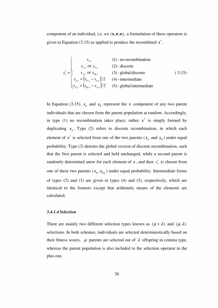
26

component of an individual, i.e. ),,,( ασxs ∈ a formulation of these operators is

given in Equation ( 3.15) as applied to produce the recombined s′ .

( )( ) teintermedia global-

teintermedia-

discrete global-

discrete-

ionrecombinat no-

)5(

)4(

)3(

)2(

)1(

2

2

or

or

,,,

,,,

,,

,,

,

−+

−+

=′

iaibjia

iaibia

ibjia

ibia

ia

i

sss

sss

ss

ss

s

s ( 3.15)

In Equation ( 3.15), as and bs represent the s component of any two parent

individuals that are chosen from the parent population at random. Accordingly,

in type (1) no recombination takes place; rather s′ is simply formed by

duplicating as . Type (2) refers to discrete recombination, in which each

element of s′ is selected from one of the two parents ( as and bs ) under equal

probability. Type (3) denotes the global version of discrete recombination, such

that the first parent is selected and held unchanged, while a second parent is

randomly determined anew for each element of s , and then is′ is chosen from

one of these two parents ( as ,jbs ) under equal probability. Intermediate forms

of types (2) and (3) are given in types (4) and (5), respectively, which are

identical to the formers except that arithmetic means of the elements are

calculated.

3.4.1.4 Selection

There are mainly two different selection types known as )( λµ + and ),( λµ

selections. In both schemes, individuals are selected deterministically based on

their fitness scores. µ parents are selected out of λ offspring in comma type,

whereas the parent population is also included to the selection operator in the

plus one.

27

Unlike ),( λµ variant, the ES)( −+ λµ always comes up with a promise of

guaranteed evolution. Since the parents are also involved in this variant, the

parent population at any generation consists of the best µ individuals sampled

thus far throughout the process. Hence, at a first sight it may seem to be more

advantageous as compared to the ES),( −λµ . According to Bäck and Schwefel

[31], [33] however, this advantage may turn into a more serious disadvantage

when interpreted in view of adaptation of the strategy parameters. They argue

that retreat from mis-adapted strategy parameters and local optima is more

difficult in the )( λµ + variant. The ratio of parent to offspring individuals

( µλ / ) is generally set to a value around 5 to 7 for a satisfactory performance

of the technique.

3.5 EVOLUTION STRATEGIES WITH DISCRETE DESIGN

VARIABLES

At the beginning, evolution strategies were developed for continuous design

spaces. However, the design of most civil engineering systems requires that the

design parameters are selected from a set of predetermined values, referred to a

discrete design set. For example, members in steel structures are selected from

profile lists given in standards. The three different approaches (reformulations)

of evolution strategies (ESs) have been proposed in the literature as extensions

of the technique for solving discrete problems: Cai and Thierauf [26], Bäck and

Schütz [27], and Rudolph [28]. Amongst them, the one proposed by Cai and

Thierauf [26] refers to a non-adaptive reformulation of the technique and has

probably found the most applications in discrete structural optimization, which

were reported in Cai and Thierauf [34], Papadrakakis and Lagaros [35],

Lagaros et al. [36], and Rajasekaran et al. [10]. The approach proposed by

Bäck and Schütz [27] corresponds to an adaptive reformulation of the

technique, which incorporates a self-adaptive strategy parameter called

mutation probability. A literature survey turns up a few recent publications

28

reporting a successful use of this approach in discrete optimum design of

structural systems (Papadrakakis et al. [37], Ebenau et al. [7]). Another

adaptive reformulation of ESs is presented by Rudolph [28] for general non-

linear mathematical optimization problems.

The evolution strategies for discrete design variables are same as ES for the

continuous design variables except the mutation algorithm.

3.5.1 Discrete Mutation

In a discrete reformulation of ESs, an individual ( I ) consists of two sets of

components, which are defined as follows:

( )sx,ΙΙ = ( 3.16)

In Equation ( 3.16), ]....[ 1 ni xxx=x stands for the design vector, and s

represents the set of strategy parameters employed by the individual for

establishing an automated problem-specific search mechanism in exploring the

design space.

Every offspring individual is subjected to mutation, resulting in a new set of

values for the design variables ( x′ ) and strategy parameters ( s′ ) of the

individual, Equation ( 3.17). This implies that not only the design information,

but also the search strategy of the individual is altered during this process.

( )s,xIs))(I(x, ′′′=mut ( 3.17)

As a general procedure, mutation of the strategy parameters is performed first.

The mutated values of the strategy parameters are then used to mutate the

29

design vector. Mutation of the design vector causes the individual to move to a

new point within the design space, and can be formulated as follows:

zxx +=′ ( 3.18)

where ],..,..[ 1 ni zzz=z refers to an n-dimensional random vector. The mutated

design vector ]....[ 1 ni xxx ′′′=x' is simply obtained by adding this random vector

to the unmutated design vector x .

3.5.2 The Approach Proposed by Bäck and Schütz

In the reformulation of technique proposed by Bäck and Schütz [27], an

individual is defined as follows:

( )s(p)x,II = ( 3.19)

where ],..,..[ 1 ni ppp=p is referred to as the vector of mutation probability, and

represents the set of adaptive strategy parameters. They are used to control

(adjust) probabilities of the design variables to undergo mutation. In its most

general formulation, each design variable ( ix ) is coupled with a separate

mutation probability ( ip ), yielding n mutation probabilities in all.

Nevertheless, it has been experimented that the general form suffers from a

poor convergence behavior, and on the contrary the algorithm exhibits a

satisfactory performance when a single mutation probability ( p ) is used for all

the design variables of an individual (Bäck and Schütz [27]). Consequently, the

number of mutation probabilities (strategy parameters) employed per

individual is set to one, i.e. ( )px,II = .

30

Mutation is performed such that the strategy parameter p is mutated first using

a logistic normal distribution, (Equation 3.20), which assures that the mutated

value of p always remains within a range (0,1).

1

)1,0(..1

1

−

−

−+=′ Ne

p

pp γ ( 3.20)

In Equation ( 3.20), p′ stands for the mutated value of p , and )1,0(N

represents a normally distributed random variable with expectation 0 and

standard deviation 1. The factor γ here refers to the learning rate of p , and is

set to the following recommended value: n21=γ . Once p′ is obtained

from Equation (3.18), the design vector ( xr

) of the individual is mutated next as

in Equation (3.19).

]1,0[if,

]1,0[if,

},..,1{

0

∈′≤

∈′>

−+−∈=

pr

pr

xnxuz

i

i

isii

i ( 3.21)

In this process, for each design variable ix a random number ir is generated

anew in a real interval [0,1]. If pri′> , the variable is not mutated, that is

0=iz and ii xx =′ . Otherwise ( pri′≤ ), it is mutated according to a uniform

distribution based variation, in which a uniformly distributed integer random

number ( iu ) sampled between 1+− ix and is xn − is assigned to iz , whereas

number of discrete values in a discrete design set. In this way, mutated value of

the design variable ( iii zxx +=′ ) is enforced to remain within 1 and sn with all

discrete values having an equal probability of being selected.

31

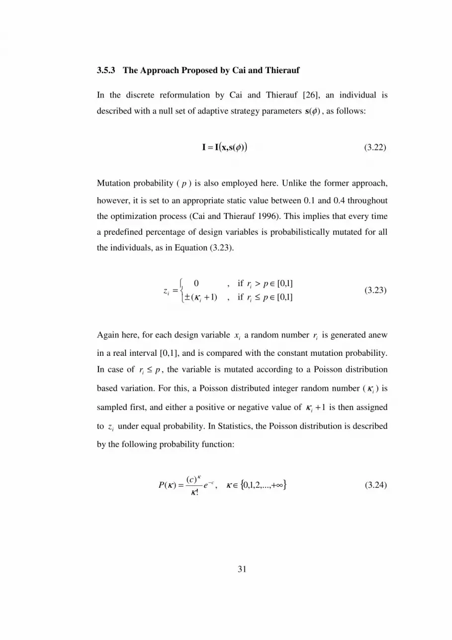
3.5.3 The Approach Proposed by Cai and Thierauf

In the discrete reformulation by Cai and Thierauf [26], an individual is

described with a null set of adaptive strategy parameters )(φs , as follows:

( ))s(x,II φ= ( 3.22)

Mutation probability ( p ) is also employed here. Unlike the former approach,

however, it is set to an appropriate static value between 0.1 and 0.4 throughout

the optimization process (Cai and Thierauf 1996). This implies that every time

a predefined percentage of design variables is probabilistically mutated for all

the individuals, as in Equation ( 3.23).

]1,0[if,

]1,0[if,

)1(

0

∈≤

∈>

+±=

pr

prz

i

i

i

i κ ( 3.23)

Again here, for each design variable ix a random number ir is generated anew

in a real interval [0,1], and is compared with the constant mutation probability.

In case of pri ≤ , the variable is mutated according to a Poisson distribution

based variation. For this, a Poisson distributed integer random number ( iκ ) is

sampled first, and either a positive or negative value of 1+iκ is then assigned

to iz under equal probability. In Statistics, the Poisson distribution is described

by the following probability function:

{ }+∞∈= − ,...,2,1,0,!

)()( κ

κκ

κce

cP ( 3.24)

32

where the parameter c corresponds to both the mean and variance of the

distribution. For some selected values of this parameter ( 15and10,8,5,3=c ),

a graphical representation of the probability distribution is plotted in Figure

3.5.

Figure 3.5 Poisson distribution for some selected values of c.

3.5.4 The Approach Proposed by Rudolph

Another adaptive reformulation of ESs is developed by Rudolph [28] for

solving general non-linear mathematical optimization problems with

unbounded integer design spaces. In this approach, mutation of a design

variable is performed based on a geometric distribution in the form of

{ }+∞∈

+−

+= ,..,2,1,0,

1

11

1

1)( ggP

g

ψψ ( 3.25)

0.00

0.05

0.10

0.15

0.20

0.25

0 5 10 15 20 25 30

c = 3

c = 5

c = 8

c = 10

c = 15

P (κ )

Poisson distributed random number (κ )

33

where g represents a geometrically distributed integer random number, and ψ

corresponds to the mean (expectation) of this particular distribution. For some

selected values of this parameter ( 40and20,10,5=ψ ), the variation in

probability distribution pattern is shown in Figure 3.6.

Figure 3.6 Geometric distribution for some selected values of ψ .

Rudolph’s approach basically rests on a variable-wise and adaptive

implementation of the parameter ψ throughout the search. The idea here is to

let each variable develop a useful probability distribution pattern of its own (by

adjusting ψ ) for successful applications of mutation. Consequently, each

design variable ix of an individual is coupled with a different { }nii ,..,2,1, ∈ψ

parameter, and the individual is described as follows:

0.00

0.02

0.04

0.06

0.08

0.10

0.12

0.14

0.16

0 20 40 60 80 100 120

s = 5

s = 10

s = 20

s = 40

P (g)

Geometrically distributed random number (g)

ψ = 5

ψ = 10

ψ = 20

ψ = 40

34

( )( )ψsx,II = ( 3.26)

For each design variable its strategy parameter is mutated by means of

Equation ( 3.27).

)1,0(.. iN

ii eτψψ =′ ( 3.27)

In Equation ( 3.27), iψ ′ stands for the mutated value of iψ . The factor τ here

refers to the learning rate of this parameter, and is set to a recommended value

of n1 for all individuals (Rudolph [28]). Then, two geometrically distributed

integer random numbers ),( 2,1, ii gg are sampled using the value of iψ ′ , and ix

is mutated by the difference of these two numbers, Equation ( 3.28).

2,1, iii ggz −= ( 3.28)

As a final point, it is worthwhile to mention that most programming language

libraries fall short of providing a function to sample the geometrically

distributed numbers 2,1, , ii gg . However, one can easily generate them using

Equation ( 3.29).

( )

′+−

−=

)1(11log

)1log(, 2,1,

i

i

ii

rgg

ψ ( 3.29)

3.5.5 A Reformulation of Rudolph’s Approach

According to Rudolph’s approach, all design variables of an individual are

subjected to mutation. When interpreted in view of discrete function

35

optimization in mathematics, this strategy is plausible, as it causes an n-

dimensional mutation of the individual to a next grid point in the vicinity of the

former. However, structural optimization problems are such that the overall

behavior of a structural system might be very sensitive to changes in a few

design variables owing to significant variations in the properties of ready

sections. For a successful operation of mutation for these problems, it is

essential to limit the number of design variables mutated at a time in an

individual, as practiced by the former approaches. To this end, a refinement of

Rudolph’s approach is accomplished in Hasançebi [38], where the parameter

p is incorporated and coupled with the original set of strategy parameters ψv

for a harmonized implementation of the mutation operator. Accordingly, in the

refined form of the Rudolph’s approach, an individual is described as follows:

( )ψ)s(p,x,II = ( 3.30)

In this framework, the parameter p is mutated first via Equation (3.18).

Analogous to former approaches, a random number [ ]1,0∈ir is then generated

anew for each design variable ix and its associated strategy parameter iψ . If

pri′> , neither ix nor iψ is mutated, i.e. ii ψψ =′ and 0=iz . If not, iψ is

mutated first according to Equation ( 3.31), and is enforced to remain greater

than 1.0 to preserve effectiveness of the mutation operator.

]1,0[if,

]1,0[if,

0.1. )1,0(. ∈′≤

∈′>

≥=′

pr

pr

e i

i

N

i

i

iiτψ

ψψ ( 3.31)

Two geometrically distributed integer random numbers ),( 2,1, ii gg are sampled

using the value of iψ ′ , and ix is mutated by the difference of these two

numbers, Equation ( 3.32).

36

]1,0[if,

]1,0[if,0

2,1, ∈′≤

∈′>

−=

pr

pr

ggz

i

i

ii

i ( 3.32)

37

CHAPTER 4

MINIMUM WEIGHT DESIGN PROBLEM FORMULATION OF STEEL FRAMES

4.1 DESIGN VARIABLES AND OBJECTIVE FUNCTION

For a steel structure consisting of mN members that are collected in dN sizing

groups and oN orientation groups for column members, the minimum weight

design problem according to ASD-AISC [39] can be posed as follows:

Find a design vector X

[ ]

Od NN

TOOOIIIX ,..,,,...,, 2121= ( 4.1)

to minimize the weight (W ) of the frame

∑∑==

=td N

j

j

N

i

ii LAW11

ρ ( 4.2)

where iρ and iA are the unit weight and area of the steel section adopted for

size group i, respectively, tN is the total number of members in size group i,

and jL is the length of the member j which belongs to group i.

The design vector X consists of dN integer values representing the sequence

numbers of steel sections assigned to dN member groups, as well as oN

38

orientation variables corresponding the orientation of the oN column groups.

The orientation design variables are represented by the state variables 0 and 1

that uses the local axes definitions defined for elements. For a column member

located along z-axis, the state variable 0 indicates that the local axis 3 of the

member is directed along y-axis, whereas the state variable 1 indicates that the

member’s local axis 3 is directed along x-axis.

Each frame element has its own element local coordinate system used to

define section properties, loads and output. The axes of this local system are

denoted 1, 2 and 3. The first axis is directed along the length of the element;

the remaining two axes lie in the plane perpendicular to the element Figure 4.1.

Figure 4.1 Element local coordinate system

4.2 AXIAL AND BENDING STRESS CONSTRAINTS

The members subjected to a combination of axial and flexural stresses must be

sized to meet the following stress constraints:

If the member is under compression and fa/Fa>0.15, the combined stress ratio is

given by the larger of,

39

00.1

11

≤−

′−

⋅+

′−

⋅+

by

ey

a

bymy

bx

ex

a

bxmx

a

a

FF

f

fC

FF

f

fC

F

f ( 4.3)

00.160.0

≤−

++

by

by

bx

bx

y

a

F

f

F

f

F

f ( 4.4)

If the member is under compression and fa/Fa≤0.15, a relatively simplified

formula is used for the combined stress ratio,

00.1 ≤−

++

by

by

bx

bx

a

a

F

f

F

f

F

f ( 4.5)

If the member is under tension, the combined stress ratio is given by,

00.1 ≤−

++

by

by

bx

bx

a

a

F

f

F

f

F

f ( 4.6)

where, Fy is the yield stress of material. The allowable axial stress and

allowable bending stress are denoted by Fa, Fb respectively. fa stands for the

computed axial stress either in compression or in tension whereas fb is the

computed normal stress in bending. The computed normal stresses about major

and minor bending directions are denoted by fbx, fby respectively. The allowable

major and minor bending stresses are represented by Fbx, Fby respectively. Cm is

the moment coefficient which is added to the equations to counterbalance

overestimation of the effect of secondary moments by the amplification factors

(1-fa/Fc’). For braced frame members there are two different Cm equations that

show difference according to the existence of transverse loading between their

ends. If there is no transverse loading between two ends than Cm is calculated

with the following formula;

40

( )21 /4.06.0 MMCm −= ( 4.7)

where M1/ M2 is the ratio of smaller end moment to the larger end moment.

)/(1 eam FfC ′+= ψ ( 4.8)

is the formulation of Cm for the frame members having transverse loading

between their ends. Ψ is a parameter that considers maximum deflection and

maximum moment in the member [39].

F’ex and F’ey are the Euler stresses about principal axes of the member which

can be formulated as,

2

2

5.2

⋅⋅

⋅=′

b

b

e

i

sK

EF

π ( 4.9)

where ib is the radius of gyration according to the plane which is perpendicular

to the bending, E is the elasticity modulus of steel, sb is the unbraced member

lengths. Finally K is the effective length K-factors about the major and minor

bending directions. For beam and bracing members, K is taken equal to unity.

For column members, alignment charts are furnished in ASD-AISC [39] for

calculation of K values for both braced and unbraced members. In this study,

however the approximate effective length formulas are given in Equation

( 4.10) and ( 4.11) are used, which are developed by Dumonteil [40]. In

Hellesland [41], a verification of these formulas is conducted, where it is

shown that these approximate formulas produce results which are accurate to

within about -1.0 and +2.0 % of exact results.

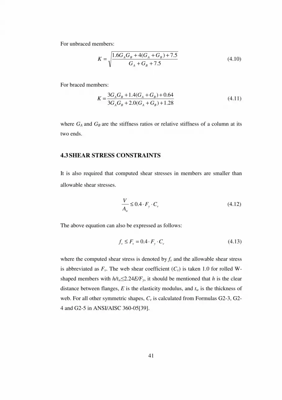
41

For unbraced members:

5.7

5.7)(46.1

++

+++=

BA

BABA

GG

GGGGK ( 4.10)

For braced members:

28.1)(0.23

64.0)(4.13

+++

+++=

BABA

BABA

GGGG

GGGGK ( 4.11)

where GA and GB are the stiffness ratios or relative stiffness of a column at its

two ends.

4.3 SHEAR STRESS CONSTRAINTS

It is also required that computed shear stresses in members are smaller than

allowable shear stresses.

vy

w

CFA

V⋅⋅≤ 4.0 ( 4.12)

The above equation can also be expressed as follows:

vyvv CFFf ⋅⋅=≤ 4.0

( 4.13)

where the computed shear stress is denoted by fv and the allowable shear stress

is abbreviated as Fv. The web shear coefficient (Cv) is taken 1.0 for rolled W-

shaped members with h/tw≤2.24E/Fy, it should be mentioned that h is the clear

distance between flanges, E is the elasticity modulus, and tw is the thickness of

web. For all other symmetric shapes, Cv is calculated from Formulas G2-3, G2-

4 and G2-5 in ANSI/AISC 360-05 [39].

42

300 200 ≤⋅

=≤⋅

= r

L K and

r

L K ten comp λ λ

4.4 SLENDERNESS CONSTRAINTS

For the elements subjected to tension and compression, the following

slenderness limitations must be satisfied according to the provisions of ASD-

AISC [39],

( 4.14)

As it is clear from the above formulations, the maximum slenderness ratio is

set to 200 for members under compression, and it is taken as 300 for tension

members. In Equation ( 4.14) L is the element buckling length and K is the

effective length factor. Minimum radius of gyration (r) is another property of

the I section member.

4.5 DISPLACEMENT AND DRIFT CONSTRAINTS

The displacement constraints are imposed such that the maximum lateral

displacements are restricted to be less than H/400, and upper limit of story drift

is set to be h/400, where H is the total height of the frame building and h is the

height of a story.

400400

hand

H≤∆≤∆ ( 4.15)

4.6 GEOMETRIC CONSTRAINTS

Finally, geometric constraints between beams and columns framing into each

other at a common joint can be considered for practicality of an optimum

solution generated. For the two beams B1 and B2 and the column shown in

Figure 4.2, one can write the following geometric constraints:

43

00.1 ≤−fc

fb

b

b ( 4.16)

( )

00.12

≤−−

′

fc

fb

td

b ( 4.17)

where fbb , fbb′ and fcb are the flange width of the beam B1, the beam B2 and

the column, respectively, cd is the depth of the column, and ft is the flange

width of the column. Equation ( 4.16) simply ensures that the flange width of

the beam B1 remains smaller than that of the column. On the other hand

Equation ( 4.17) enables that flange width of the beam B2 remains smaller than

clear distance between the flanges of the column )2( fc td − .

bfb

bfcb'fb

B1

B2

dc

tf

Figure 4.2 Beam-column geometric constraints

44

CHAPTER 5

OPTIMIZATION ALGORITHM AND SOFTWARE

In this chapter, the ES algorithm developed for optimum design of steel space

frames is discussed, where size and orientation variables are used together to

minimize the structural weight of the systems. The resulting algorithm is

computerized in a software called OFES. The capabilities and practical features

of the software are also discussed later in the chapter.

5.1 A GENERAL FLOWCHART

The general flowchart which outlines the major computational steps of the ES

algorithm developed in the study is presented in Figure 5.1. Concerning this

flowchart, the first two steps consist of setting the generation counter t to 0, and

of creating an initial population )0(P . The initial population consists of µ

number of parent individuals, which are customarily created through a random

initialization. Hence, it is high likely that the initial population consists of a

high number of unfit individuals that violate the constraints or highly

overestimate the optimum. The next step is to evaluate the individuals’

performances, where each individual is assigned a fitness score according to

how well it satisfies the objective function and constraints of a problem at

hand. In the following step, an offspring population )(tP′ is created through a

sequential application of recombination and mutation operators to the parent

population. The offspring population consists of λ number of individuals,

which also undergo evaluation process (step 5) to attain fitness scores. After

evaluating the offspring population, selection (step 6) is implemented to

determine the survivors, which in fact form the parent population of the next

45

generation, i.e. )1( +tP . A (µ,λ)-ES selection is implemented, where the

parents are not included in the selection mechanism; instead selection is carried

out by choosing the µ best individuals out of λ offspring in reference to the

individuals’ fitness scores. This completes one generation in optimization

procedure, accompanied by the increase of generation counter by one (step 7).

The surviving individuals in generation t make up the parent population

)1( +tP of the next generation. The loop between the steps 4 and 8 is iterated

in the same way for each new value of the generation counter until a

termination criterion is satisfied.

Begin the process

Step 1: t := 0; Set the generation counter to 0

Step 2: initialize P (0); Create an initial population with µ parent individuals

Step 3: evaluate P (0); Evaluate the initial population P (0)

Step 4: P’ (t ):=recom and mut P (t ); Create an offspring population with λ individuals by recombining and mutating the parent population

Step 5: evaluate P’ (t ); Evaluate the offspring population

Step 6: P (t +1):=select from P’ (t ); Select the µ best individuals from offspring population only

Terminate the process

Step 7: t := t + 1; Increase generation counter by one

Step 8: if termination criterion is

satisfied?

YES

NO

Figure 5.1 General flowchart of the ES algorithm developed in the study.

46

5.2 DETAILED ALGORITHM

The optimization routine discussed above forms the basic framework of the

solution algorithm developed in the study. In the following subsections,

computational implementations and further details of this algorithm are

explained.

5.2.1 Initial Population

Initial population consists of µ number of parent solutions (individuals). Apart

from a vector of size design variables I and a vector of orientation design

variables O , each individual incorporates three sets of strategy parameters

( sp , op ,ψ ), Equation ( 5.1). All the strategy parameters are self-adaptive by

nature, and are employed by the individual for establishing a problem-specific

search scheme in an automated manner.

),,,,( ψOIJJ os pp= ( 5.1)

In Equation (5.1), sp and op refer to the mutation probability parameters used

for size and orientation variables, respectively. They are used to tune the

overall mutability of the individual for size and orientation variables. The

vector ψ represents the whole set of geometric distribution parameters iψ

),..,1( dNi = , such that each size design variable in an individual is coupled

with a different iψ to change online the shape and flatness of the geometric

distribution used to mutate it. A random initialization of population is

implemented for the design vectors, and the strategy parameters are assigned to

appropriate values initially ()0(

sp ,)0(

op)0(

iψ ) based on numerical

experimentation. In the numerical examples discussed in Chapter 6, the

47

following initial values are used for the strategy parameter: )0(

sp = 0.25,

)0(

op =0.25 and 20)0( =iψ .

5.2.2 Evaluation of Population

The initial population is measured (evaluated) next. Here, each individual is

analyzed in conjunction with an external structural analysis package SAP2000

with the set of steel sections selected for the design variables and orientations

assigned for column groups and force and deformation responses are obtained

under the applied loads. Objective function values of the feasible solutions that

satisfy all the problem constraints are directly calculated from Equation ( 4.2).

However, infeasible solutions that violate some of the problem constraints are

penalized using external penalty function approach, and their objective

function values are calculated according to Equation ( 5.2).

[ ]

+=+= ∑

=

jn

j

jgWJPenaltyW1

)(1)(1 αφ ( 5.2)

In Equation ( 5.2), φ is the constrained objective function value, dj njg ,..1, =

represents the whole set of normalized constraints, and α is the penalty

coefficient used to tune the intensity of penalization as a whole. Although α

can be assigned to an appropriate static value, such as 1=α , an adaptive

penalty function implementation is favored by letting this parameter adjust its

value automatically during the search for the most efficient optimization

process (Hasançebi [42] [34]). In this implementation, α is permitted to adjust

itself automatically during the search, as formulated in Equation ( 5.3):

48

infeasibleis)1(if

feasibleis)1(if

)1(.

)1(.)/1()(

−

−

−

−=

tb

tb

tf

tft

α

αα ( 5.3)

where )(tα and )1( −tα denote the penalty coefficients at generations t and t-1

respectively, )1( −tb is the best design at generation t-1, and f is an arbitrary

constant referred to as the learning rate parameter of α . Experiments with

various test problems indicate that the optimal value of f equals to 1.1.

The rationale behind Equation ( 5.3) is to continually enforce the algorithm to

adopt a search direction along the constraint boundaries. If the best individual

at the preceding generation is infeasible, the penalty is intensified somewhat in

order to render the feasible regions more attractive for individuals, and thereby

guiding the search towards these regions. If, however, the best individual at the

preceding generation is infeasible, this time the search is directed towards

infeasible regions by relaxing the penalty to some extent. The overall

consequence of this action is that the search is carried out very close to

constraint boundaries throughout the optimization process. As to be discussed

in the numerical examples, another significant feature of the adaptive penalty

function is that it avoids entrapment of the search at a local optimum, which is

often the case observed when a static penalty function is utilized.

5.2.3 Recombination

After evaluated, the parent population undergoes recombination and mutation

operators to yield the offspring population. Recombination provides a trade of

design information between the µ parents to generate λ new (offspring)

individuals. Recombination is not only to design vectors ( I and O ), but also

to the strategy parameters ( sp , op ,ψ ) of the individuals in a variety of

different schemes. In the present study a global discrete recombination operator

49

is utilized for size and orientation design variables, whereas strategy

parameters are recombined using intermediate scheme. Given that s represents

an arbitrary component of an individual, i.e., { }ψIs ,,,, os ppO∈ , the

recombined s′ can be formulated as follows:

teintermedia:

discrete global:

2/)(

or

−+=′

a

i

b

i

a

i

bj

i

a

i

i

sss

sss ( 5.4)

In Equation ( 5.4), as and bs refer to the s component of two parent

individuals which are chosen randomly from the parent population, and a

is and

b

is represent typical elements of as and bs . In global discrete recombination,

a

is is chosen from the two parents under equal probability such that the first

parent is held unchanged, whereas the second parent is chosen a new for each

element of i. In intermediate recombination scheme, both parents are kept

fixed for all elements of i and their arithmetic means are calculated.

5.2.4 Mutation

Every offspring individual of the form ),,,,( ψOIJJ os pp= is subject to

mutation, which results in a new (and expectantly improved) set of design

variables ( OI ′′, ) and strategy parameters ( ψ′′′ ,, os pp ) for the individual. The

application of mutation to size and orientation design variables is performed in

a different manner, and is explained in the following.

5.2.4.1 Mutation of Size Variables and Strategy Parameters

The mutation of size design variables is performed as follows. First, the size

mutation probability parameter sp is mutated for an individual using a logistic

50

normal distribution (Equation 5.5), which ensures that the mutated value of sp

always remains within a range (0,1).

1

)1,0(..1

1

−

−

−+=′ N

s

s

sse

p

pp

γ ( 5.5)

A random number r is then generated between the range [0,1] for each size

design variable iI and its associated iψ parameter. If spr ′> , neither iI nor iψ

is mutated. Otherwise, iψ is mutated according to a lognormal distribution

based variation (Equation 5.6).

]1,0[if0.1. )1,0(. ∈′≤≥=′s

N

ii pre iτψψ ( 5.6)

Finally, two geometrically distributed integer random numbers ),( 2,1, ii zz are

sampled using the distribution parameter iψ ′ , and iI is mutated by the

difference of them, Equation ( 5.7).

)()( 2,1, iiiiii zzII ψψ ′−′+=′ ( 5.7)

In Equations (5.5-5.7), sp′ , iψ ′ and iI ′ are the mutated values of their

corresponding parameters, )1,0(N is a normally distributed random variable

with expectation 0 and standard deviation 1, sγ and τ are the learning rate

constants for sp and iψ , which are usually set to recommended values of

ds N21=γ and dN1 , respectively where dN stands for the number of

size design variables.

51

5.2.4.2 Mutation of Orientation Variables and Strategy Parameters

Again, for the mutation of orientation design variables, first strategy parameter

op is mutated using a logistic normal distribution (Equation 5.8).

1

)1,0(..1

1

−

−

−+=′ N

o

o

ooe

p

pp

γ ( 5.8)

Similar to the definitions given for Equations (5.5-5.7), in Equation ( 5.8), op′

represents the mutated value of op , )1,0(N is a normally distributed random

variable with expectation 0 and standard deviation 1, and oγ is the learning

rate constants for op , which is set to the value oo N21=γ , where oN

stands for the number of orientation design variables employed for column

groups.

For each orientation variable iO , a random number r is generated between the

range [0,1]. If pr ′> , the variable is not mutated. Otherwise, iO is mutated as

follows:

]1,0[if)( ∈′≤=′oii proswitcho ( 5.9)

The )( ioswitch operator in Equation ( 5.9) replaces the current value of the

state variable with the other character in the set, i.e., if [ ] 0)1( ==iOswitch or

[ ] 1)0( ==iOswitch . As a result of this, the orientations of the columns

belonging to i-th column group are changed as a whole.

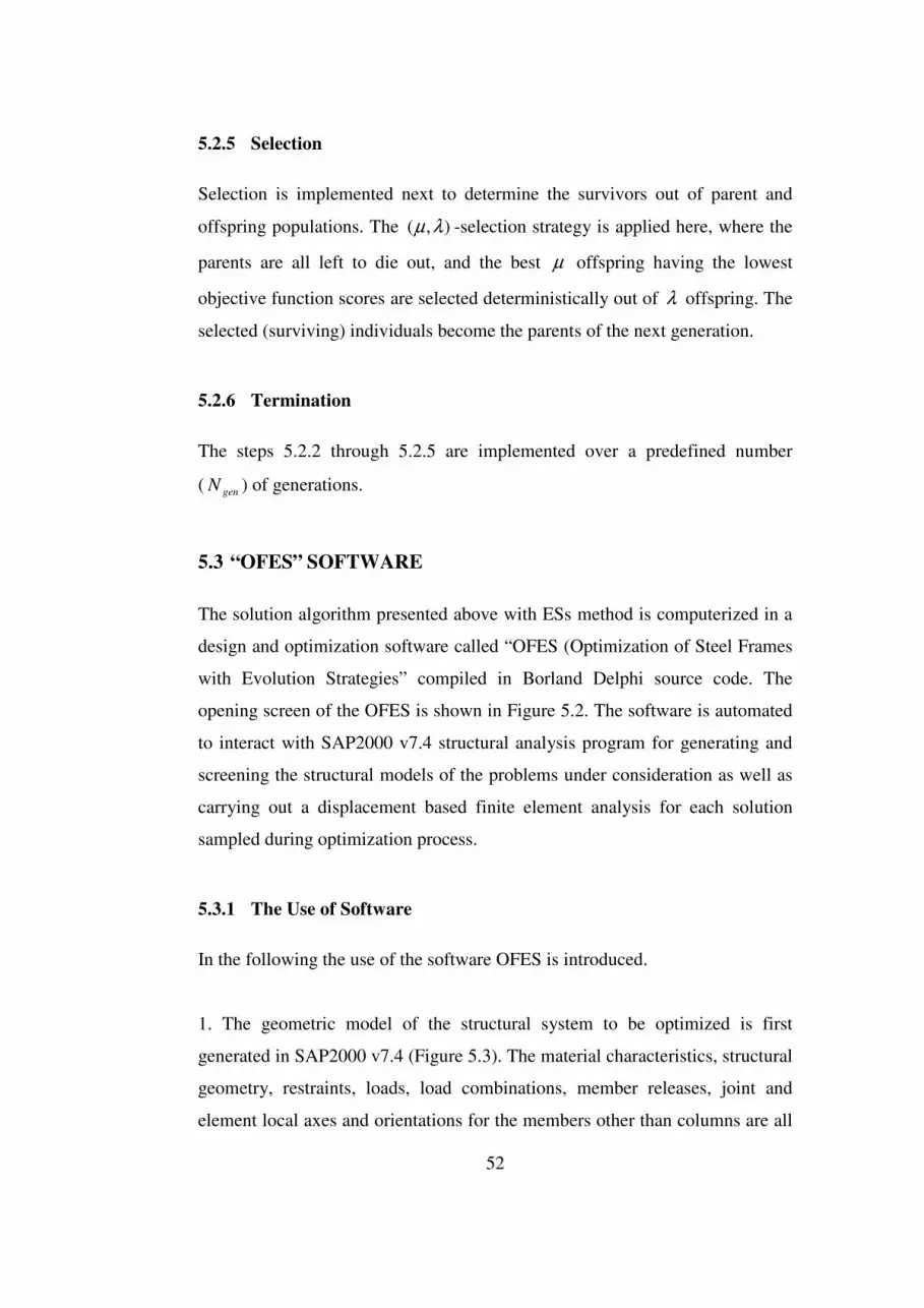
52

5.2.5 Selection

Selection is implemented next to determine the survivors out of parent and

offspring populations. The ),( λµ -selection strategy is applied here, where the

parents are all left to die out, and the best µ offspring having the lowest

objective function scores are selected deterministically out of λ offspring. The

selected (surviving) individuals become the parents of the next generation.

5.2.6 Termination

The steps 5.2.2 through 5.2.5 are implemented over a predefined number

( genN ) of generations.

5.3 “OFES” SOFTWARE

The solution algorithm presented above with ESs method is computerized in a

design and optimization software called “OFES (Optimization of Steel Frames

with Evolution Strategies” compiled in Borland Delphi source code. The

opening screen of the OFES is shown in Figure 5.2. The software is automated

to interact with SAP2000 v7.4 structural analysis program for generating and

screening the structural models of the problems under consideration as well as

carrying out a displacement based finite element analysis for each solution

sampled during optimization process.

5.3.1 The Use of Software

In the following the use of the software OFES is introduced.

1. The geometric model of the structural system to be optimized is first

generated in SAP2000 v7.4 (Figure 5.3). The material characteristics, structural

geometry, restraints, loads, load combinations, member releases, joint and

element local axes and orientations for the members other than columns are all

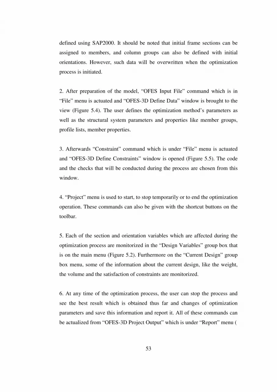
53

defined using SAP2000. It should be noted that initial frame sections can be

assigned to members, and column groups can also be defined with initial

orientations. However, such data will be overwritten when the optimization

process is initiated.

2. After preparation of the model, “OFES Input File” command which is in

“File” menu is actuated and “OFES-3D Define Data” window is brought to the

view (Figure 5.4). The user defines the optimization method’s parameters as

well as the structural system parameters and properties like member groups,

profile lists, member properties.

3. Afterwards “Constraint” command which is under “File” menu is actuated

and “OFES-3D Define Constraints” window is opened (Figure 5.5). The code

and the checks that will be conducted during the process are chosen from this

window.

4. “Project” menu is used to start, to stop temporarily or to end the optimization

operation. These commands can also be given with the shortcut buttons on the

toolbar.

5. Each of the section and orientation variables which are affected during the

optimization process are monitorized in the “Design Variables” group box that

is on the main menu (Figure 5.2). Furthermore on the “Current Design” group

box menu, some of the information about the current design, like the weight,

the volume and the satisfaction of constraints are monitorized.

6. At any time of the optimization process, the user can stop the process and

see the best result which is obtained thus far and changes of optimization

parameters and save this information and report it. All of these commands can

be actualized from “OFES-3D Project Output” which is under “Report” menu (

54

Figure 5.6). In addition, the changes in optimization parameters can be

monitorized from “Watch Parameters” group box throughout the iterations

without stopping the process (Figure 5.2).

7. In accordance to the request, with the help of the “View” menu SAP2000 is

employed and the best design is extrude viewed (Figure 5.7 ).

Figure 5.2 Opening screen of OFES

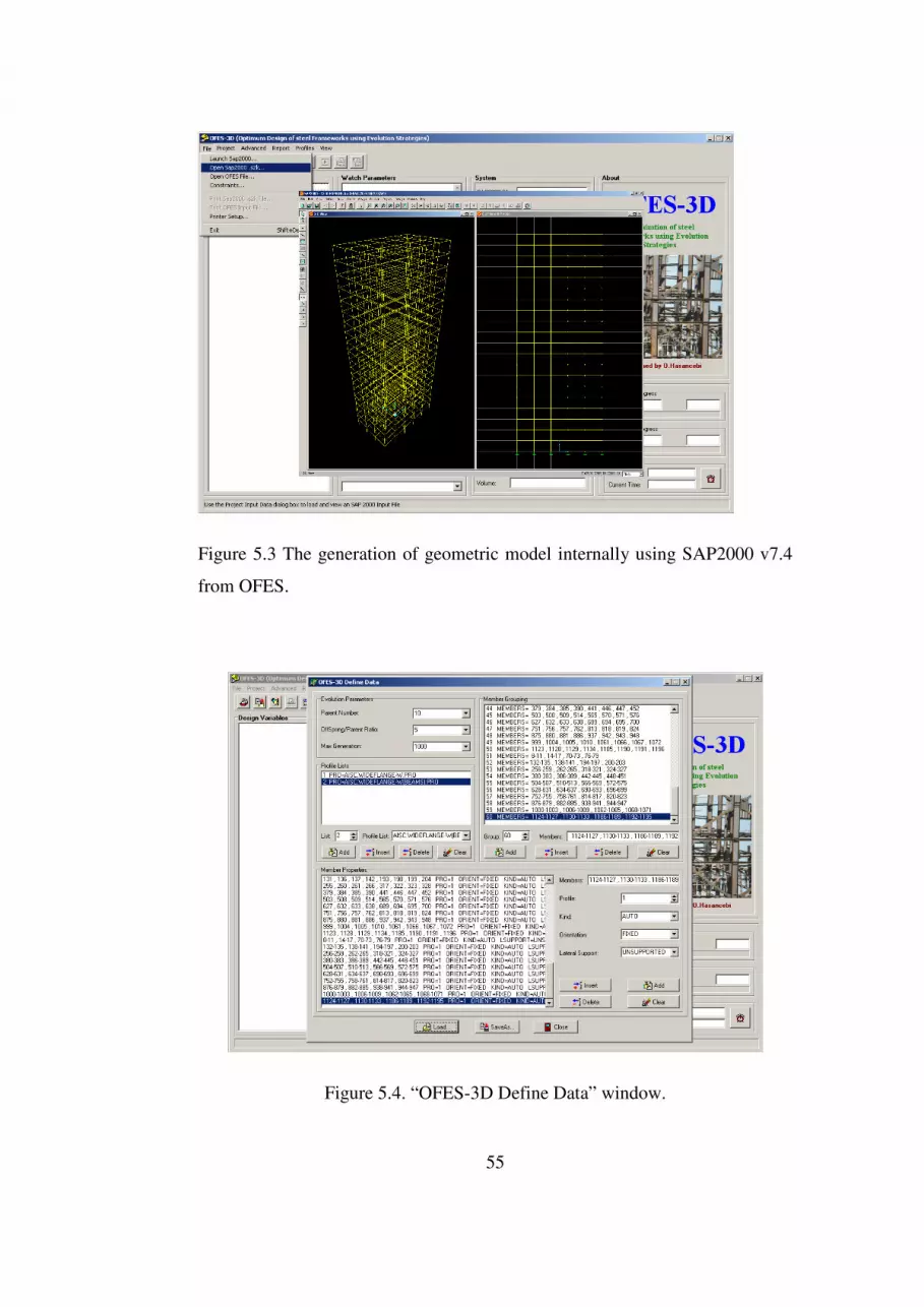
55

Figure 5.3 The generation of geometric model internally using SAP2000 v7.4

from OFES.

Figure 5.4. “OFES-3D Define Data” window.

56

Figure 5.5“OFES-3D Define Constraint” window.

Figure 5.6“OFES-3D Project Output” window.

57

Figure 5.7 Extruded view of the best design.

5.3.2 Practical Features of Ofes

OFES has the following practical features:

1. Structural designs can be performed according to TS648 and ASD-AISC

design provisions.

2. Steel structural systems can be modeled in both 2 and 3 dimension.

3. Optimum design can be performed according to the following checks which

take place in the valid codes:

- Bending and axial stress checks

- Slenderness ratio check

- Maximum displacement check

- Story drift check.

- Shear stress check

58

- Beam column connection compliance check.

4. The following conditions can be considered during the design of structural

systems in OFES:

- Statical analysis of the structure under single and combined loads.

- Dynamic analysis of the structure with response spectrum and mode

superposition methods.

- Modeling of slabs with shell elements in 2 dimensional finite element

models.

- Modeling of hinged and semi-rigid column and beam connections.

- Modeling of elastic soils with springs.

- Employment of rigid diaphragms for each floor in their own planes.

5. The following practical conditions can be considered during design of

structural systems in OFES:

- Optimum designs can be obtained for both of the systems that

sidesway is prevented or permitted.

- All types of diagonal connection members (X, V-type, etc.) can be

defined to carry the lateral loads.

- It is possible to define desired number of groups and each of the

members in the same group may have the same section and

orientation.

- Allowable bending stresses of the beam members can be calculated to

the consideration of laterally supported to torsion or not.

- All profile lists which are prescribed in Eurocode and AISC can be

used in solutions.

- Column orientations can be defined as design variables and so the

required column orientations can be assigned for optimum design.

59

CHAPTER 6

DESIGN EXAMPLES

6.1 INTRODUCTION

The effect of column orientation on minimum weight design of steel structures

is investigated using four numerical examples designed according to the

provisions of ASD-AISC specification. In these examples, first steel structures

are sized for minimum weight considering the size design variables only,

where orientations of the column members are initially assigned and kept

unchanged during optimization process. Next, the weight optimum design of

structures are implemented using both size and orientation design variables.

General properties of design examples are tabulated in Table 6-1.

Table 6-1 General properties of design examples

Design Examples 960 Member

Steel Frame

568 Member

Steel Frame

1230 Member

Steel Frame

3590 Member

Steel Frame

Number of stories 10 10 10 30

Types of members Column and

beam

Column and

beam

Column, beam

and bracing

Column, beam

and bracing

Plan view of the system Square Square Rectangular Non-symmetrical

Design loads Gravity and

wind loads

Gravity and

wind loads

Gravity and

wind loads

Gravity and wind

loads

Number of size variables 45 33 50 129

Number of orientation

variables 7 7 7 16

Number of analyses for

size variables 3 3 3 3

Number of analyses for size

and orientation variables5 5 5 5

60

6.2 DESIGN LOADS

Load cases and combinations are determined according to the ASCE 7-05,

(Minimum Design Loads for Buildings and Other Structures) [43]. The

structures are subjected to both gravity (GL) and lateral (LL) loads. Gravity

loads include dead, live and snow loads and they are defined identically for all

of the structures considered in the study. As for the lateral loading, the

structure is subjected to horizontal wind forces. The gravity and lateral forces

are combined under nine loading conditions which are tabulated in Table 6-2.

Table 6-2 Load Combinations

Combination Load Cases

1 1.0GL + 1.0LL-x

2 1.0GL + 1.0LL-y

3 1.0GL + 0.75LL-x + MT

4 1.0GL + 0.75LL-x - MT

5 1.0GL + 0.75LL-y + MT

6 1.0GL + 0.75LL-y - MT

7 1.0GL + 0.75LL-x + 0.75LL-y

8 1.0GL + 0.563LL-x + 0.563LL-y + MT

9 1.0GL + 0.563LL-x + 0.563LL-y - MT

The load combinations are defined according to the cases that are stated in

ASCE 7-05 [43] which are shown in Figure 6.1. In case 1, full design wind

pressure acting on the projected area perpendicular to each principal axis of the

structure is considered separately along each principal axis. For the 2nd case,

75% of the design wind pressure acting on the projected area perpendicular to

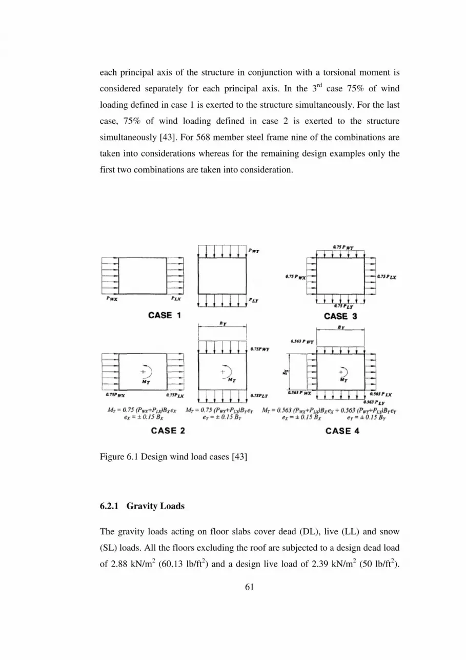
61

each principal axis of the structure in conjunction with a torsional moment is

considered separately for each principal axis. In the 3rd case 75% of wind

loading defined in case 1 is exerted to the structure simultaneously. For the last

case, 75% of wind loading defined in case 2 is exerted to the structure

simultaneously [43]. For 568 member steel frame nine of the combinations are

taken into considerations whereas for the remaining design examples only the

first two combinations are taken into consideration.

Figure 6.1 Design wind load cases [43]

6.2.1 Gravity Loads

The gravity loads acting on floor slabs cover dead (DL), live (LL) and snow

(SL) loads. All the floors excluding the roof are subjected to a design dead load

of 2.88 kN/m2 (60.13 lb/ft2) and a design live load of 2.39 kN/m2 (50 lb/ft2).

62

The roof is subjected to a design dead load of 2.88 kN/m2 (60.13 lb/ft2) plus

snow load. The design snow load is computed using the following equation in

ASCE 7-05 [43] :

gtess IpCCCp 7.0= ( 6.1)

where sp is the design snow load in kN/m2, sC is the roof slope factor, eC is

the exposure factor, tC is the temperature factor, I is the importance factor,

and gp is the ground snow load. For a heated building having a flat and fully

exposed roof, these factors may be chosen as follows: 0.1=sC , 9.0=eC ,

0.1=tC , 0.1=I , and 20.1=gp kN/m2 (25 lb/ft2), resulting in a design snow

load of 1.20 kN/m2 (25 lb/ft2). The calculated gravity loads are applied as

uniformly distributed loads on the beams using distribution formulas developed

for two way slabs.

6.2.2 Lateral Wind Loads

The design wind loads are also computed according to ASCE 7-05 [43] using

the following equations in two unit systems:

))(613.0( 2pdztzw GCIVKKKp = in N/m2 ( 6.2)

))(00256.0( 2pdztzw GCIVKKKp = in lb/ft2 ( 6.3)

where wp is the design wind pressure, zK is the velocity exposure coefficient,

ztK is the topographic factor, dK is the wind direction factor, V is the basic

wind speed, G is the gust factor, and pC is the external pressure coefficient.

63

The velocity exposure coefficient ( zK ) for a story is calculated using one of

the two formulas given in Equations (6.4) and (6.5) based on the elevation of

the story.

For z<15ft )/2()/15(*01.2 alpha

gz zK = ( 6.4)

15ft≤z≤zg )/2()/(*01.2 alpha

gz zzK =

( 6.5)

where gz is the nominal height of the atmospheric boundary layer used in the

standard and alpha is the 3-s-gust-speed power law exponent and both of the

variables are taken from Table 6.2 in [43]. It should be underlined that

Equations ( 6.4) and (6.5) are used to find the design wind pressure on

windward face, along which the wind pressure increases with height. On the

leeward face, the magnitude of the negative wind pressure is assumed to be

constant. To calculate wp on leeward face, zK term in Equation (6.4) or (6.5)

is replaced with hK , which is calculated from Equation (6.6)

)/2()/(*01.2 alpha

gh zhK = ( 6.6)

where h is the total height of the building.

Assuming that the structures are located in an urban area with a basic wind

speed of 94.46=V m/s (105 mph) and exposure category B, the following

values are used for these parameters: 0.1=ztK , 85.0=dK , 0.1=I , 85.0=G ,

ftzg 1200= , 7=alpha and 8.0=pC for windward face and -0.5 for leeward

face,. The calculated wind loads are applied as uniformly distributed lateral

loads on the external beams of the frames located on windward and leeward

facades at every floor level.

64

6.3 PROFILE LIST AND MATERIAL PROPERTIES

The wide-flange (W) profile list consisting of 297 ready sections is used to size

column members in the design examples. On the other hand, beams and

diagonals are selected from discrete sets of 171 and 147 economical sections

selected from wide-flange profile list based on area and inertia properties in the

former, and on area and radii of gyration properties in the latter. In all the

design examples, the following material properties of the steel are used:

modulus of elasticity (E) = 29000ksi (203893.6MPa) and yield stress ( yF ) =

36ksi (253.1MPa).

6.4 ES PARAMETERS

In all the design examples, the parameters of the discrete evolution strategy

method employed are set to the following values for an efficient optimum

design process: population parameters ( 10=µ , 60=λ ), initial values of the

strategy parameters ( 25.0)0(

=sp , 25.0)0(

=op , 20)0( =iψ ), and maximum

generation number ( 1000=genN ).It follows that a total of 60000 structural

analyses are performed in each example to obtain the optimum designs

reported in the paper.

6.5 DESIGN EXAMPLE 1: 960 MEMBER STEEL FRAME

In this example it is intended to examine the effect of intensity of lateral

loading on optimal layout of column orientations. A 10 story 5x5 bay regular

steel space frame consisting of 960 members is taken as the base for the

application (Figure 6.2). The structure is designed under four different wind

force cases such that in addition to a regular basic wind speed of 105mph, the

building is subjected to wind forces calculated based on basic wind speeds of

90, 120 and 150 mph. The gravity loading and initial column orientations are

defined the same in all the test cases. Two design studies are carried out for

65

each test case depending on the type of design variables included in the

optimization process. First, the structure is designed for minimum weight

considering the size design variables only, where initial orientations of the

column members are kept unchanged. Second, size and orientation design

variables are employed together to minimize the weight of the frame. The

results obtained in each case are compared and optimal layout of column

orientations is investigated.

6.5.1 Structural System

The 10-story steel space frame consists of 960 members and 396 joints. It has

five bays in x-direction and five bays in y-direction with a regular bay spacing

of 15ft (4.57m), and the story height is equal to 12ft (3.66m). Hence, the

structural system occupies a space of 75x75ft2 (522.58m2) in plan and 120ft

(36.58m) in elevation. Figure 6.2 shows 3D, plan and side views of this

structure. The stability of the structure is provided with moment resisting

connections and columns are fixed to the foundation.

To satisfy practical fabrication requirements, 960 members of the frame are

collected under 45 member size groups (size design variables); 35 column size

groups and 10 beam size groups. The member groups are clearly tabulated in

Table 6-3. The grouping of the members is performed both in plan and

elevation levels. In plan level, columns are collected under seven groups

considering the symmetry of the structure about x and y axes as shown in

Figure 6.3. Four corner columns are placed in first group. The second and third

groups are the outer columns in x-z direction and in y-z direction, respectively.

Inner columns are divided into four groups that are inner corner columns (4th),

inner x-z direction columns (5th), inner y-z direction columns (6th) and the

central columns (7th). On the other hand, beams are collected under two groups

as outer and inner beams in plan level grouping. In elevation level grouping, it

is enabled that member groups have the same sections in every two stories

66

The orientation variables are assigned keeping in mind that all the successive

columns along the frame height (i.e., columns that that lie on the vertical line)

must have the same orientation for practical requirements. Hence, each column

group shown in Figure 6.3 is associated with one orientation variable. Thus, a

total of seven orientation variables are defined in the problem.

(a) 3D view

67

(b) Plan view

(c) Side view

68

(d) Side view

Figure 6.2 960 member steel frame

Load cases and combinations are determined according to the ASCE 7-05 [43],

as explained in Section 6.2. In this example only one design case is studied.

The 1st and the 2nd combinations that are tabulated in Table 6-2 are taken into

consideration for this design case. The resulting gravity loading on the beams

of roof and floors is tabulated in Table 6-4 and the wind loadings on windward

and leeward faces of the frame calculated based on different basic wind speeds

are presented in Table 6-5 and Table 6-6.

69


Table 6-3 Member grouping for 960 member steel frame.

Member

Group Group Name

Member

Group Group Name

1 1st &2nd floor corner columns 24 7th &8th floor inner columns

in x-z direction

2 3rd &4th floor corner columns 25 9th &10th floor inner columns

in x-z direction

3 5th &6th floor corner columns 26 1st &2nd floor inner columns

in y-z direction

4 7th &8th floor corner columns 27 3rd &4th floor inner columns

in y-z direction

5 9th&10th floor corner columns 28 5th &6th floor inner columns

in y-z direction

6 1st &2nd floor outer columns

in x-z direction 29

7th &8th floor inner columns

in y-z direction

7 3rd &4th floor outer columns

in x-z direction 30

9th &10th floor inner columns

in y-z direction

70

Table 6-3 (continued)

Member

Group Group Name

Member

Group Group Name

8 5th &6th floor outer columns

in x-z direction 31 1st &2nd floor inner columns


in x-z direction 32 3rd &4th floor inner columns


in x-z direction 33 5th &6th floor inner columns

11 1st &2nd floor outer columns

in y-z direction 34 7th &8th floor inner columns

12 3rd &4th floor outer columns

in y-z direction 35 9th &10th floor inner columns


in y-z direction 36 1st &2nd floor outer beams


in y-z direction 37 3rd &4th floor outer beams


in y-z direction 38 5th &6th floor outer beams

16 1st &2nd floor inner corner

columns 39 7th &8th floor outer beams

17 3rd &4th floor inner corner

columns 40 9th &10th floor outer beams

18 5th &6th floor inner corner

columns 41 1st &2nd floor inner beams


columns 42 3rd &4th floor inner beams


columns 43 5th &6th floor inner beams

21 1st &2nd floor inner columns

in x-z direction 44 7th &8th floor inner beams

22 3rd &4th floor inner columns

in x-z direction 45 9th &10th floor inner beams

23 5th &6th floor inner columns

in x-z direction

71

Table 6-4 Gravity loading on the beams of 960 member steel frame.

Uniformly Distributed Load

Outer Beams Inner Beams Beam Type

kN/m (lb/ft) kN/m (lb/ft)

Roof Beams 5.54 (379.4) 11.08 (758.8)

Floor Beams 8.04 (550.65) 16.08 (1101.3)

Table 6-5 Wind Loading Values under Wind Speeds of 90mph and 105mph (in

kN/m, lb/ft)

Floor Z(ft) V=90mph V=105mph

Windward Leeward Windward Leeward

1 12 1,21 (82,66) 1,37 (93,58) 1,64 (112,5) 1,86 (127,4)

2 24 1,38 (94,54) 1,37 (93,58) 1,88 (128,7) 1,86 (127,4)

3 36 1,55 (106,2) 1,37 (93,58) 2,11 (144,5) 1,86 (127,4)

4 48 1,68 (115,2) 1,37 (93,58) 2,29 (156,9) 1,86 (127,4)

5 60 1,79 (122,8) 1,37 (93,58) 2,44 (167,2) 1,86 (127,4)

6 72 1,89 (129,4) 1,37 (93,58) 2,57 (176,1) 1,86 (127,4)

7 84 1,97 (135,2) 1,37 (93,58) 2,69 (184,1) 1,86 (127,4)

8 96 2,05 (140,5) 1,37 (93,58) 2,79 (191,2) 1,86 (127,4)

9 108 2,12 (145,3) 1,37 (93,58) 2,89 (197,8) 1,86 (127,4)

10 120 1,09 (74,87) 0,68 (46,79) 1,49 (101,9) 0,93 (63,69)

72

Table 6-6 Wind Loading Values under Wind Speeds of 120mph and 150mph

(in kN/m, lb/ft)

Floor Z

(ft) V=120mph V=150mph

Windward Leeward Windward Leeward

1 12 2,15 (146,9) 2,43 (166,4) 3,35 (229,6) 3,8 (260)

2 24 2,45 (168,1) 2,43 (166,4) 3,83 (262,6) 3,8 (260)

3 36 2,76 (188,7) 2,43 (166,4) 4,3 (294,9) 3,8 (260)

4 48 2,99 (204,9) 2,43 (166,4) 4,67 (320,1) 3,8 (260)

5 60 3,19 (218,4) 2,43 (166,4) 4,98 (341,2) 3,8 (260)

6 72 3,36 (230) 2,43 (166,4) 5,25 (359,4) 3,8 (260)

7 84 3,51 (240,4) 2,43 (166,4) 5,48 (375,6) 3,8 (260)

8 96 3,65 (249,7) 2,43 (166,4) 5,7 (390,2) 3,8 (260)

9 108 3,77 (258,3) 2,43 (166,4) 5,89 (403,6) 3,8 (260)

10 120 1,94 (133,1) 1,21 (83,18) 3,04 (208) 1,9 (130)

In each of the four test cases, the wide-flange (W) profile list consisting of 297

ready sections is used to size column members and beams are selected from

discrete sets of 171 economical sections selected from wide-flange profile list

based on area and inertia properties. Provisions of ASD-AISC [39] are taken

into consideration for the stress, stability, and geometric constraints.

Displacements of all the joints in x and y directions are limited to 9.15cm

(3.6in), and the upper limit of inter story drifts is set to 0.91cm (0.36in)

6.5.2 Test Results

For each case of the basic wind speeds (that is, V = 90, 105, 120 and 150 mph)

a total of eight independent runs are performed considering the stochastic

73

nature of the ES technique. First, three independent runs are conducted to

minimize the weight of the frame using size variables only. Next, additional

five runs are implemented where size variables are used together with

orientation variables simultaneously to minimize the frame weight.

6.5.2.1 The Case for Basic Wind Speed of 90=V mph

The results of the eight runs produced for the basic wind speed case of

90=V mph are tabulated in Table 6-7 in terms of the minimum weight and

volume of the frame attained in each run. The design history curves obtained in

these runs are plotted in Figure 6.4, which show the improvement of the

feasible best design during the search process in each run. The number of

structural analyses performed is shown in the horizontal axis in this graph,

whereas the vertical axis represents the variation of the best feasible design

weights obtained thus far during the search.

It is seen from Table 6-7 or Figure 6.4, the best design weight of 465,884.61lb

(211,325.26 kg) is obtained when the frame is sized for minimum weight under

initial choice of column orientations. When column orientations are permitted

to vary in the optimization process, the best design weight of the frame has

been improved to 438,602.37lb (198,950.035kg). The sectional designations

attained for member groups in both design cases are compared in Table 6-8.

The optimal layout of the column orientation achieved in the latter case is

shown in Figure 6.5. It follows that the optimal layout of column orientations

can lead to a reduction as much as 5.9 % in the frame weight.

74

400000

500000

600000

700000

800000

900000

1000000

50 100 200 400 600 800 900 950 1000

Number of Structural Analysis

Bes

t F

easi

be

Des

ign

Wei

gh

t

Test 1

Test 2

Test 3

Test 1

Test 2

Test 3

Test 4

Test 5



frame in eight runs for the basic wind speed case of 90=V mph

Columns with fixed orientations Columns with varying orientations

Test 1 Test 2 Test 3 Test1 Test2 Test3 Test4 Test5

Total

Weight 473747,71 474685 465884,6 438602,4 448927,3 444330,1 440614,3 474839,5

Total

Volume 1674020,2 1677332,1 1646235,4 1549831,7 1586315,5 1570070,9 1556941 1677877,9

Columns with fixed orientation

Columns with varying orientation

75


for the basic speed wind case of 90=V mph.

Best design with initial column

orientations

Best design with varying column

orientations Group

Number Ready Section Area (cm2), (in2) Ready Section Area (cm2), (in2)

1 W12X53 100,64 (15,6) W8X48 90,97 (14,1)

2 W10X49 92,9 (14,4) W10X45 85,81 (13,3)

3 W10X33 62,645 (9,71) W10X33 62,645 (9,71)

4 W8X31 58,903 (9,13) W14X34 64,52 (10)

5 W8X24 45,677 (7,08) W8X24 45,677 (7,08)

6 W14X99 187,74 (29,1) W12X65 123,23 (19,1)

7 W12X65 123,23 (19,1) W10X54 101,94 (15,8)

8 W12X58 109,68 (17) W10X49 92,9 (14,4)

9 W10X45 85,81 (13,3) W8X35 66,45 (10,3)

10 W8X31 58,903 (9,13) W12X26 49,355 (7,65)

11 W14X74 140,64 (21,8) W18X76 143,87 (22,3)

12 W12X65 123,23 (19,1) W10X60 113,55 (17,6)

13 W10X49 92,9 (14,4) W10X49 92,9 (14,4)

14 W12X40 76,13 (11,8) W12X40 76,13 (11,8)

15 W8X31 58,903 (9,13) W12X26 49,355 (7,65)

16 W14X109 206,45 (32) W14X109 206,45 (32)

17 W12X96 181,94 (28,2) W12X96 181,94 (28,2)

18 W10X77 145,81 (22,6) W18X76 143,87 (22,3)

19 W12X53 100,64 (15,6) W10X49 92,9 (14,4)

20 W10X49 92,9 (14,4) W8X28 53,226 (8,25)

21 W14X109 206,45 (32) W21X111 210,97 (32,7)

22 W14X99 187,74 (29,1) W14X90 170,97 (26,5)

23 W12X79 149,68 (23,2) W12X72 136,13 (21,1)

24 W12X53 100,64 (15,6) W10X54 101,94 (15,8)

25 W8X31 58,903 (9,13) W8X28 53,226 (8,25)

26 W24X131 248,39 (38,5) W14X109 206,45 (32)

27 W14X90 170,97 (26,5) W14X99 187,74 (29,1)

76

Table 6-8 (cntinued)


orientations


orientations Group


28 W12X72 136,13 (21,1) W12X72 136,13 (21,1)

29 W10X49 92,9 (14,4) W12X53 100,64 (15,6)

30 W8X28 53,226 (8,25) W8X28 53,226 (8,25)

31 W14X120 227,74 (35,3) W14X99 187,74 (29,1)

32 W14X90 170,97 (26,5) W14X90 170,97 (26,5)

33 W12X72 136,13 (21,1) W12X65 123,23 (19,1)

34 W12X65 123,23 (19,1) W12X53 100,64 (15,6)

35 W8X31 58,903 (9,13) W12X30 56,71 (8,79)

36 W8X18 33,935 (5,26) W14X22 41,871 (6,49)

37 W14X22 41,871 (6,49) W14X22 41,871 (6,49)

38 W14X22 41,871 (6,49) W14X22 41,871 (6,49)

39 W6X16 30,581 (4,74) W8X18 33,935 (5,26)

40 W6X15 28,581 (4,43) W6X12 22,903 (3,55)

41 W16X26 49,548 (7,68) W12X26 49,355 (7,65)

42 W14X26 49,613 (7,69) W16X26 49,548 (7,68)

43 W16X26 49,548 (7,68) W14X22 41,871 (6,49)

44 W14X22 41,871 (6,49) W14X22 41,871 (6,49)

45 W8X18 33,935 (5,26) W8X18 33,935 (5,26)

Weight 465,884.61 lb (211,325.26 kg) 438,602.37lb (198,950.035kg).

77


the basic speed wind case of 90=V mph.





these runs are plotted in Figure 6.6. It is seen from Table 6-9 or Figure 6.6 that

the best design weight of 507,432.09lb (230,171.196kg) is obtained when the

frame is sized for minimum weight under initial choice of column orientations.

When column orientations are permitted to vary in the optimization process,

the best design weight of the frame has been improved to 473,395.61lb

(214,732.25 kg). The sectional designations attained for member groups in

both design cases are compared in Table 6-10. The optimal layout of the

column orientation achieved in the latter case is shown in Figure 6.7. It follows

78

that the optimal layout of column orientations can lead to a reduction as much

as 6.7 % in the frame weight.

400000

500000

600000

700000

800000

900000

1000000

50 100 200 400 600 800 900 950 1000


Bes

t F

easi

be

Des

ign

Wei

gh

t

Test 1

Test 2

Test 3

Test 1

Test 2

Test 3

Test 4

Test 5





frame in eight runs for the basic wind speed case of 105=V mph


Test1 Test2 Test3 Test1 Test2 Test3 Test4 Test5

Total

Weight 513907,2 507432,1 539275,7 473395,6 490608,0 485069,8 489478,0 496842,7

Total

Volume 1815926,4 1793046,2 1905567,8 1672776 1733597,3 1714027,7 1729604,2 1755627,8

79




orientations


orientations Group


1 W8X40 75,48 (11,7) W12X65 123,23 (19,1)

2 W10X39 74,19 (11,5) W10X54 101,94 (15,8)

3 W10X33 62,645 (9,71) W14X43 81,29 (12,6)

4 W12X30 56,71 (8,79) W10X33 62,645 (9,71)

5 W12X26 49,355 (7,65) W12X26 49,355 (7,65)

6 W14X90 170,97 (26,5) W12X65 123,23 (19,1)

7 W12X72 136,13 (21,1) W12X58 109,68 (17)

8 W12X65 123,23 (19,1) W10X49 92,9 (14,4)

9 W10X49 92,9 (14,4) W10X39 74,19 (11,5)

10 W8X31 58,903 (9,13) W12X26 49,355 (7,65)

11 W16X67 127,1 (19,7) W12X65 123,23 (19,1)

12 W12X65 123,23 (19,1) W12X58 109,68 (17)

13 W10X54 101,94 (15,8) W10X49 92,9 (14,4)

14 W10X39 74,19 (11,5) W8X40 75,48 (11,7)

15 W8X31 58,903 (9,13) W8X24 45,677 (7,08)

16 W14X120 227,74 (35,3) W18X130 246,45 (38,2)

17 W10X112 212,26 (32,9) W14X99 187,74 (29,1)

18 W12X87 165,16 (25,6) W14X90 170,97 (26,5)

19 W12X58 109,68 (17) W12X58 109,68 (17)

20 W8X31 58,903 (9,13) W8X31 58,903 (9,13)

21 W24X131 248,39 (38,5) W14X109 206,45 (32)

22 W14X109 206,45 (32) W14X90 170,97 (26,5)

23 W12X87 165,16 (25,6) W12X79 149,68 (23,2)

24 W12X58 109,68 (17) W12X58 109,68 (17)

25 W8X31 58,903 (9,13) W8X31 58,903 (9,13)

26 W36X150 285,16 (44,2) W24X117 221,94 (34,4)

80



orientations


orientations Group


27 W14X109 206,45 (32) W14X99 187,74 (29,1)

28 W12X79 149,68 (23,2) W12X79 149,68 (23,2)

29 W10X54 101,94 (15,8) W12X53 100,64 (15,6)

30 W8X31 58,903 (9,13) W16X40 76,13 (11,8)

31 W14X132 250,32 (38,8) W14X109 206,45 (32)

32 W14X99 187,74 (29,1) W14X99 187,74 (29,1)

33 W18X97 183,87 (28,5) W12X79 149,68 (23,2)

34 W12X58 109,68 (17) W12X53 100,64 (15,6)

35 W8X31 58,903 (9,13) W12X30 56,71 (8,79)

36 W16X26 49,548 (7,68) W14X22 41,871 (6,49)

37 W16X26 49,548 (7,68) W14X22 41,871 (6,49)

38 W14X22 41,871 (6,49) W8X18 33,935 (5,26)

39 W8X18 33,935 (5,26) W8X18 33,935 (5,26)

40 W6X15 28,581 (4,43) W6X16 30,581 (4,74)

41 W18X35 66,45 (10,3) W16X31 58,839 (9,12)

42 W12X26 49,355 (7,65) W16X31 58,839 (9,12)

43 W16X26 49,548 (7,68) W16X26 49,548 (7,68)

44 W16X26 49,548 (7,68) W14X22 41,871 (6,49)

45 W8X21 39,742 (6,16) W8X21 39,742 (6,16)

Weight 507,432.09lb (230,171.20kg) 473395.61lb (214735.25kg)

81


the basic speed wind cases of 105=V and 120 mph.





these runs are plotted in Figure 6.8. It is seen from Table 6-11 or Figure 6.8

that the best design weight of 553,079.62 lb (250,876.92 kg) is obtained when

the frame is sized for minimum weight under initial choice of column

orientations. When column orientations are permitted to vary in the

optimization process, the best design weight of the frame has been improved to

532,413.88lb (241,502.94kg). The sectional designations attained for member

groups in both design cases are compared in Table 6-12. The optimal layout of

the column orientation achieved in the latter case is exactly identical to the one

82

obtained for the basic wind speed case of 105=V (Figure 6.7). It follows that

the optimal layout of column orientations can lead to a reduction as much as

3.7 % in the frame weight.

500000

600000

700000

800000

900000

1000000

1100000

50 100 200 400 600 800 900 950 1000

Number of Structural Analy sis

Bes

t Fea

sibe

Des

ign

Wei

ght

Test 1

Test 2

Test 3

Test 1

Test 2

Test 3

Test 4

Test 5




83





Total

Weight 553079,62 594861,83 580816,66 543948,32 548797 541722,04 610655,27 532413,88

Total

Volume 1954345 2101985,28 2052355,7 1922078,88 1939212 1914212,2 2157792,5 1881321,1




orientations


orientations Group

Number Ready Section Area (cm2),(in2) Ready Section Area(cm2), (in2)

1 W8X48 90,97 (14,1) W16X67 127,1 (19,7)

2 W14X48 90,97 (14,1) W12X50 94,84 (14,7)

3 W8X31 58,903 (9,13) W14X43 81,29 (12,6)

4 W12X26 49,355 (7,65) W8X40 75,48 (11,7)

5 W8X21 39,742 (6,16) W8X24 45,677 (7,08)

6 W14X90 170,97 (26,5) W14X68 129,03 (20)

7 W12X79 149,68 (23,2) W16X67 127,1 (19,7)

8 W12X65 123,23 (19,1) W10X49 92,9 (14,4)

9 W10X49 92,9 (14,4) W8X40 75,48 (11,7)

10 W8X31 58,903 (9,13) W12X26 49,355 (7,65)

11 W18X97 183,87 (28,5) W12X72 136,13 (21,1)

12 W12X79 149,68 (23,2) W12X65 123,23 (19,1)

13 W16X67 127,1 (19,7) W14X68 129,03 (20)

14 W14X48 90,97 (14,1) W14X43 81,29 (12,6)

15 W8X31 58,903 (9,13) W8X28 53,226 (8,25)

16 W14X132 250,32 (38,8) W40X149 282,58 (43,8)

17 W12X106 201,29 (31,2) W14X109 206,45 (32)

84



orientations


orientations Group

Number Ready Section Area (cm2),(in2) Ready Section Area(cm2), (in2)

18 W12X96 181,94 (28,2) W12X79 149,68 (23,2)

19 W12X53 100,64 (15,6) W27X84 160 (24,8)

20 W8X31 58,903 (9,13) W8X31 58,903 (9,13)

21 W14X145 275,48 (42,7) W33X152 288,39 (44,7)

22 W14X109 206,45 (32) W14X109 206,45 (32)

23 W14X90 170,97 (26,5) W21X111 210,97 (32,7)

24 W14X90 170,97 (26,5) W12X65 123,23 (19,1)

25 W10X49 92,9 (14,4) W8X35 66,45 (10,3)

26 W12X152 288,39 (44,7) W24X117 221,94 (34,4)

27 W14X109 206,45 (32) W14X99 187,74 (29,1)

28 W10X88 167,1 (25,9) W12X96 181,94 (28,2)

29 W12X87 165,16 (25,6) W12X58 109,68 (17)

30 W8X31 58,903 (9,13) W10X33 62,645 (9,71)

31 W14X159 301,29 (46,7) W21X122 231,61 (35,9)

32 W14X109 206,45 (32) W14X120 227,74 (35,3)

33 W14X90 170,97 (26,5) W14X90 170,97 (26,5)

34 W10X60 113,55 (17,6) W12X65 123,23 (19,1)

35 W8X31 58,903 (9,13) W8X31 58,903 (9,13)

36 W16X26 49,548 (7,68) W14X26 49,613 (7,69)

37 W16X26 49,548 (7,68) W14X22 41,871 (6,49)

38 W16X26 49,548 (7,68) W14X22 41,871 (6,49)

39 W12X26 49,355 (7,65) W14X22 41,871 (6,49)

40 W8X18 33,935 (5,26) W6X15 28,581 (4,43)

41 W16X31 58,839 (9,12) W16X31 58,839 (9,12)

42 W14X30 57,097 (8,85) W21X44 83,87 (13)

43 W14X26 49,613 (7,69) W12X26 49,355 (7,65)

44 W16X31 58,839 (9,12) W16X26 49,548 (7,68)

45 W10X22 41,871 (6,49) W8X21 39,742 (6,16)

Weight 553,079.62lb (250,876.92kg) 532,413.88lb (241,502.94kg)

85





these runs are plotted in Figure 6.9. It is seen from Table 6-13 or Figure 6.9

that the best design weight of 660,182.4 lb (299,458.74 kg) is obtained when

the frame is sized for minimum weight under initial choice of column

orientations. When column orientations are permitted to vary in the

optimization process, the best design weight of the frame has been improved to

604,324.86lb (274,121.76kg). The sectional designations attained for member

groups in both design cases are compared in Table 6-14. The optimal layout of

the column orientation achieved in the latter case is shown Figure 6.10. It

follows that the optimal layout of column orientations can lead to a reduction

as much as 8.5 % in the frame weight.

86

500000

600000

700000

800000

900000

1000000

1100000

1200000

50 100 200 400 600 800 900 950 1000


Bes

t F

easi

be

Des

ign

Wei

gh

t

Test 1

Test 2

Test 3

Test 1

Test 2

Test 3

Test 4

Test 5






Total

Weight 747817,54 660182,4 662060,25 604324,86 617909,54 612631,74 631117,26 618032,2

Total

Volume 2642464,8 2332800 2339435,5 2135423,52 2183425,9 2164776,5 2230096,3 2183859,4



87




orientations


orientations Group

Number Ready Section Area(cm2) ,(in2) Ready Section Area(cm2), (in2)

1 W21X62 118,06 (18,3) W12X65 123,23 (19,1)

2 W10X39 74,19 (11,5) W12X53 100,64 (15,6)

3 W16X40 76,13 (11,8) W8X48 90,97 (14,1)

4 W14X30 57,097 (8,85) W8X31 58,903 (9,13)

5 W8X24 45,677 (7,08) W8X24 45,677 (7,08)

6 W14X145 275,48 (42,7) W12X87 165,16 (25,6)

7 W24X104 197,42 (30,6) W12X65 123,23 (19,1)

8 W12X65 123,23 (19,1) W12X58 109,68 (17)

9 W12X65 123,23 (19,1) W14X48 90,97 (14,1)

10 W10X45 85,81 (13,3) W12X26 49,355 (7,65)

11 W27X94 178,71 (27,7) W16X100 189,68 (29,4)

12 W18X86 163,23 (25,3) W12X72 136,13 (21,1)

13 W16X67 127,1 (19,7) W10X60 113,55 (17,6)

14 W10X49 92,9 (14,4) W10X49 92,9 (14,4)

15 W8X31 58,903 (9,13) W10X33 62,645 (9,71)

16 W40X192 364,52 (56,5) W14X145 275,48 (42,7)

17 W14X132 250,32 (38,8) W14X132 250,32 (38,8)

18 W14X109 206,45 (32) W12X106 201,29 (31,2)

19 W14X90 170,97 (26,5) W12X65 123,23 (19,1)

20 W12X65 123,23 (19,1) W14X43 81,29 (12,6)

21 W12X170 322,58 (50) W14X132 250,32 (38,8)

22 W40X192 364,52 (56,5) W14X145 275,48 (42,7)

23 W14X99 187,74 (29,1) W14X99 187,74 (29,1)

24 W12X79 149,68 (23,2) W16X67 127,1 (19,7)

25 W10X45 85,81 (13,3) W10X39 74,19 (11,5)

26 W14X176 334,19 (51,8) W30X173 327,74 (50,8)

27 W27X146 276,77 (42,9) W12X136 257,42 (39,9)

28 W14X145 275,48 (42,7) W14X90 170,97 (26,5)

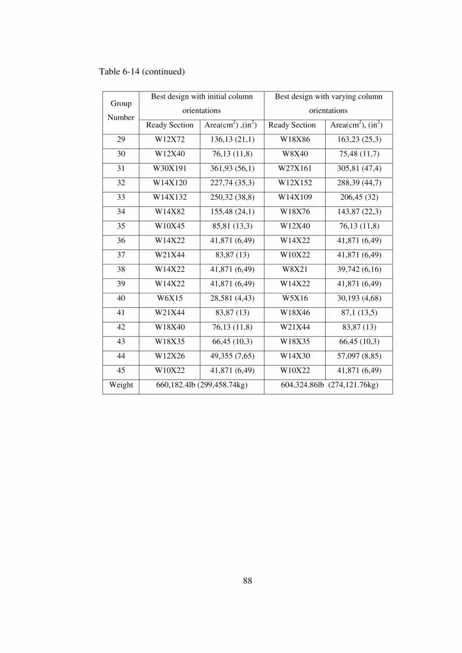
88



orientations


orientations Group

Number Ready Section Area(cm2) ,(in2) Ready Section Area(cm2), (in2)

29 W12X72 136,13 (21,1) W18X86 163,23 (25,3)

30 W12X40 76,13 (11,8) W8X40 75,48 (11,7)

31 W30X191 361,93 (56,1) W27X161 305,81 (47,4)

32 W14X120 227,74 (35,3) W12X152 288,39 (44,7)

33 W14X132 250,32 (38,8) W14X109 206,45 (32)

34 W14X82 155,48 (24,1) W18X76 143,87 (22,3)

35 W10X45 85,81 (13,3) W12X40 76,13 (11,8)

36 W14X22 41,871 (6,49) W14X22 41,871 (6,49)

37 W21X44 83,87 (13) W10X22 41,871 (6,49)

38 W14X22 41,871 (6,49) W8X21 39,742 (6,16)

39 W14X22 41,871 (6,49) W14X22 41,871 (6,49)

40 W6X15 28,581 (4,43) W5X16 30,193 (4,68)

41 W21X44 83,87 (13) W18X46 87,1 (13,5)

42 W18X40 76,13 (11,8) W21X44 83,87 (13)

43 W18X35 66,45 (10,3) W18X35 66,45 (10,3)

44 W12X26 49,355 (7,65) W14X30 57,097 (8,85)

45 W10X22 41,871 (6,49) W10X22 41,871 (6,49)

Weight 660,182.4lb (299,458.74kg) 604,324.86lb (274,121.76kg)

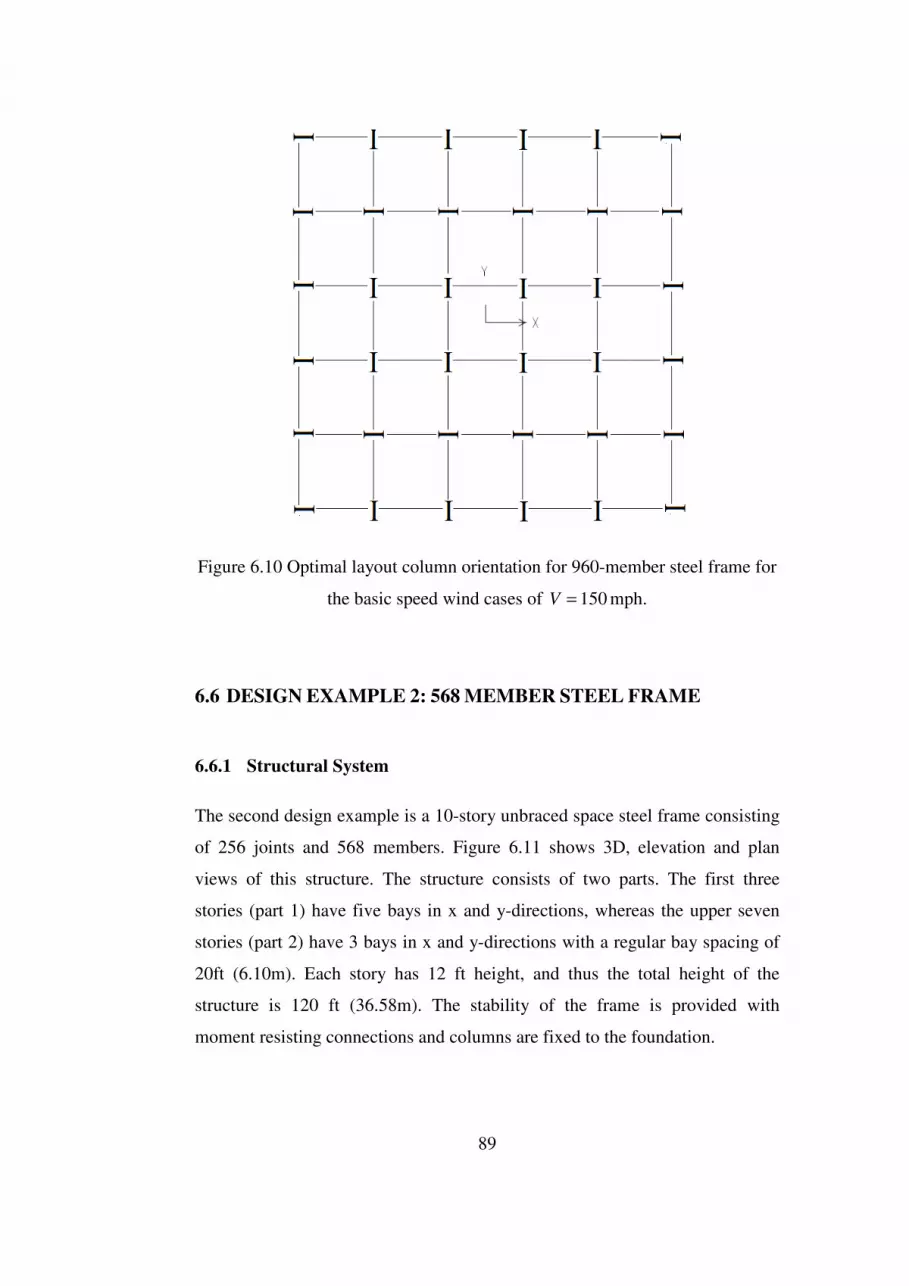
89


the basic speed wind cases of 150=V mph.



The second design example is a 10-story unbraced space steel frame consisting

of 256 joints and 568 members. Figure 6.11 shows 3D, elevation and plan

views of this structure. The structure consists of two parts. The first three

stories (part 1) have five bays in x and y-directions, whereas the upper seven

stories (part 2) have 3 bays in x and y-directions with a regular bay spacing of

20ft (6.10m). Each story has 12 ft height, and thus the total height of the

structure is 120 ft (36.58m). The stability of the frame is provided with

moment resisting connections and columns are fixed to the foundation.

90


collected under 33 member size groups; 23 column size groups and 10 beam

size groups. The member groups are clearly tabulated in Table 6-15. The

grouping of the members is performed both in plan and elevation levels. A plan

level grouping of columns for the parts 1 and 2 are shown in Figure 6.12. On

the other hand, beams are collected under two groups as outer and inner beams

in plan level grouping. In elevation level grouping, it is enabled that the

member groups in the three stories in the first part have the same sections, and

member groups have the same sections in every two stories in the second part.

The orientation variables are assigned, bearing in mind that all the successive

columns along the frame height must have the same orientation. Hence, each

column group in Figure 6.12 is associated with an orientation variable,

resulting in seven orientation variables in all.

The structure is analyzed for two different design cases. For the first design

case the 1st and the 2nd combinations that are tabulated in Table 6-2 are taken

into consideration. For the second design case, the structural system is

designed for 9 combinations (Table 6-2). The load cases and combinations are

determined according to the ASCE 7-05 [43], as explained in Section 6.2. The

resulting gravity loading on the beams of roof and floors is tabulated in Table

6-16 and the wind loadings on windward and leeward faces of the frame

calculated based on a basic wind speed of 105mph (46.94 m/s) is presented in

Table 6-17. Torsional moment values. MT, are calculated according to ASCE

7-05 [43] and tabulated in Table 6-18. ). A joint is defined at the center of

gravity of each story and the calculated torsional moment values are applied at

these joints. It is crucial to mention that diaphragm constraints are also defined

between all the joints of the floor systems to distribute the torsional moments

equivalently.

91


column members, and beams are selected from discrete sets of 171 economical

sections selected from wide-flange profile list based on area and inertia

properties. Provisions of ASD-AISC [39] are taken into consideration for the

stress, stability, and geometric constraints. Displacements of all the joints in x

and y directions are limited to 9.15cm (3.6in), and the upper limit of inter story

drifts is set to 0.91cm (0.36in).

Two design cases are studied for each of the two cases. First, the structure is

designed for minimum weight considering the size design variables only,

where initial orientations of the column members are kept unchanged. Second,

size and orientation variables are employed together to minimize the weight of

the frame.

Table 6-15 Member grouping for 568 member steel frame

Member

Group Group Name

Member

Group Group Name

1 1st 2nd & 3rd floor corner

columns 18

10th floor columns in y-z

direction

2 1st 2nd & 3rd floor outer

columns in x-z direction 19

1st 2nd & 3rd floor inner

columns

3 1st 2nd & 3rd floor outer

columns in y-z direction 20

4th &5th floor inner

columns

4 1st 2nd & 3rd floor inner

corner columns 21


columns

5 4th &5th floor corner

columns 22


columns


columns 23 10th floor inner columns


columns 24

1st 2nd & 3rd floor outer

beams

92


Member

Group Group Name

Member

Group Group Name

8 10th floor corner columns 25 1st 2nd & 3rd floor inner

beams


columns in x-z direction 26 4th &5th floor outer beams

10 4th &5th floor columns in x-

z direction 27 6th &7th floor outer beams


z direction 28 8th &9th floor outer beams


z direction 29 10th floor outer beams

13 10th floor inner columns in

x-z direction 30 4th &5th floor inner beams


columns in y-z direction 31 6th &7th floor inner beams

15 4th &5th floor columns in y-

z direction 32 8th &9th floor inner beams


z direction 33 10th floor inner beams


z direction

93

(a) 3D view

(b) Plan view of 5x5 bay

94

(c) Plan view of 3x3 bay

(d) Side view


95

(a)Part 1

(b) Part 2

Figure 6.12 Grouping of members of 568-member steel frame in plan level

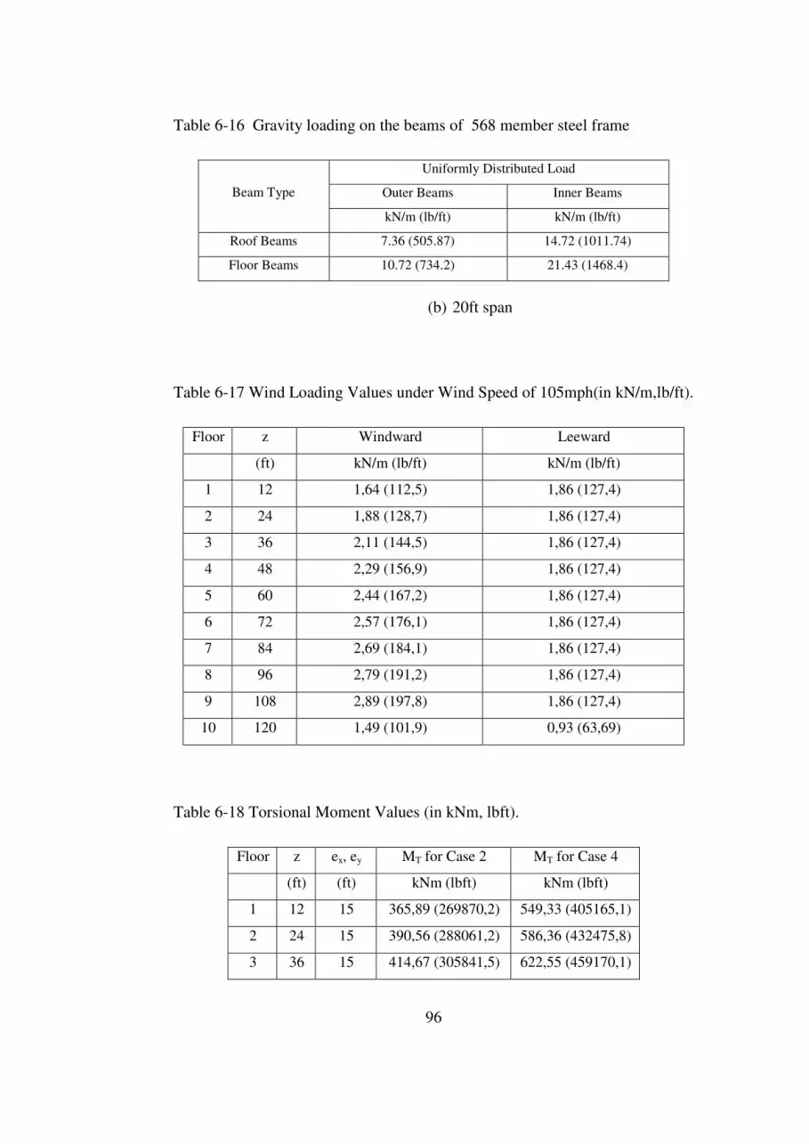
96

Table 6-16 Gravity loading on the beams of 568 member steel frame


Outer Beams Inner Beams Beam Type

kN/m (lb/ft) kN/m (lb/ft)

Roof Beams 7.36 (505.87) 14.72 (1011.74)

Floor Beams 10.72 (734.2) 21.43 (1468.4)

(b) 20ft span

Table 6-17 Wind Loading Values under Wind Speed of 105mph(in kN/m,lb/ft).

Floor z Windward Leeward

(ft) kN/m (lb/ft) kN/m (lb/ft)

1 12 1,64 (112,5) 1,86 (127,4)

2 24 1,88 (128,7) 1,86 (127,4)

3 36 2,11 (144,5) 1,86 (127,4)

4 48 2,29 (156,9) 1,86 (127,4)

5 60 2,44 (167,2) 1,86 (127,4)

6 72 2,57 (176,1) 1,86 (127,4)

7 84 2,69 (184,1) 1,86 (127,4)

8 96 2,79 (191,2) 1,86 (127,4)

9 108 2,89 (197,8) 1,86 (127,4)

10 120 1,49 (101,9) 0,93 (63,69)

Table 6-18 Torsional Moment Values (in kNm, lbft).

Floor z ex, ey MT for Case 2 MT for Case 4

(ft) (ft) kNm (lbft) kNm (lbft)

1 12 15 365,89 (269870,2) 549,33 (405165,1)

2 24 15 390,56 (288061,2) 586,36 (432475,8)

3 36 15 414,67 (305841,5) 622,55 (459170,1)

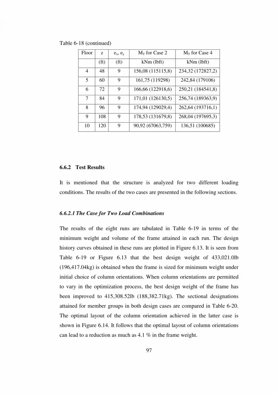
97


Floor z ex, ey MT for Case 2 MT for Case 4

(ft) (ft) kNm (lbft) kNm (lbft)

4 48 9 156,08 (115115,8) 234,32 (172827,2)

5 60 9 161,75 (119298) 242,84 (179106)

6 72 9 166,66 (122918,6) 250,21 (184541,8)

7 84 9 171,01 (126130,5) 256,74 (189363,9)

8 96 9 174,94 (129029,4) 262,64 (193716,1)

9 108 9 178,53 (131679,8) 268,04 (197695,3)

10 120 9 90,92 (67063,759) 136,51 (100685)

6.6.2 Test Results

It is mentioned that the structure is analyzed for two different loading

conditions. The results of the two cases are presented in the following sections.

6.6.2.1 The Case for Two Load Combinations

The results of the eight runs are tabulated in Table 6-19 in terms of the

minimum weight and volume of the frame attained in each run. The design

history curves obtained in these runs are plotted in Figure 6.13. It is seen from

Table 6-19 or Figure 6.13 that the best design weight of 433,021.0lb

(196,417.04kg) is obtained when the frame is sized for minimum weight under








98

400000

450000

500000

550000

600000

650000

700000

50 100 200 400 600 800 900 950 1000


Bes

t F

easi

be

Des

ign

Wei

gh

t (l

b)

Test 1

Test 2

Test 3

Test 1

Test 2

Test 3

Test 4

Test 5



Figure 6.13 Design history graph of 568 member steel frame


member frame in eight runs.



Total

Weight 446910,9 433021,0 457038,57 415936,1 418030,7 415308,52 419646,1 448392,6

Total

Volume 1579190,4 1530109,4 1614977,3 1469738,9 1477140,4 1467521,3 1482848,6 1584426,2

99



orientations


orientations Group

Number Ready Section Area (cm2) (in2) Ready Section Area (cm2) (in2)

1 W10X49 92,9 (14,4) W14X48 90,97 (14,1)

2 W8X58 110,32 (17,1) W8X40 75,48 (11,7)

3 W21X68 129,03 (20) W14X43 81,29 (12,6)

4 W12X87 165,16 (25,6) W18X97 183,87 (28,5)

5 W12X58 109,68 (17) W10X60 113,55 (17,6)

6 W12X53 100,64 (15,6) W10X49 92,9 (14,4)

7 W10X39 74,19 (11,5) W8X40 75,48 (11,7)

8 W14X22 41,871 (6,49) W10X26 49,097 (7,61)

9 W27X146 276,77 (42,9) W27X146 276,77 (42,9)

10 W14X99 187,74 (29,1) W14X90 170,97 (26,5)

11 W14X90 170,97 (26,5) W16X67 127,1 (19,7)

12 W10X60 113,55 (17,6) W12X53 100,64 (15,6)

13 W10X39 74,19 (11,5) W10X30 57,032 (8,84)

14 W12X106 201,29 (31,2) W14X120 227,74 (35,3)

15 W14X90 170,97 (26,5) W14X90 170,97 (26,5)

16 W12X79 149,68 (23,2) W14X90 170,97 (26,5)

17 W14X61 115,48 (17,9) W10X54 101,94 (15,8)

18 W8X28 53,226 (8,25) W12X26 49,355 (7,65)

19 W40X215 408,39 (63,3) W40X192 364,52 (56,5)

20 W14X176 334,19 (51,8) W14X159 301,29 (46,7)

21 W14X109 206,45 (32) W14X109 206,45 (32)

22 W12X65 123,23 (19,1) W12X79 149,68 (23,2)

23 W12X26 49,355 (7,65) W8X24 45,677 (7,08)

24 W14X22 41,871 (6,49) W12X19 35,935 (5,57)

25 W18X35 66,45 (10,3) W18X35 66,45 (10,3)

26 W16X26 49,548 (7,68) W16X26 49,548 (7,68)

27 W16X26 49,548 (7,68) W14X22 41,871 (6,49)

100



orientations


orientations Group


28 W16X26 49,548 (7,68) W16X26 49,548 (7,68)

29 W12X19 35,935 (5,57) W12X19 35,935 (5,57)

30 W21X44 83,87 (13) W24X55 104,52 (16,2)

31 W18X35 66,45 (10,3) W18X35 66,45 (10,3)

32 W16X31 58,839 (9,12) W14X30 57,097 (8,85)

33 W14X22 41,871 (6,49) W12X22 41,806 (6,48)

Weight 433,021.0lb (196,417.04kg) 415,308.52lb (188,382.71kg)

(a) Part 1

101

(a) Part 2


6.6.2.2 The Case for Nine Load Combinations




Table 6-21or Figure 6.15 that the best design weight of 442,643.3lb

(200,781.68kg) is obtained when the frame is sized for minimum weight under








102

400000

450000

500000

550000

600000

650000

700000

50 100 200 400 600 800 900 950 1000


Bes

t F

easi

be

Des

ign

Wei

gh

t (l

b)

Test 1

Test 2

Test 3

Test 1

Test 2

Test 3

Test 4

Test 5






Total

Weight 442643,3 463366,5 446818,0 430086,8 445404,7 438915,3 439932,5 462253,2

Total

Volume 1564110,7 1637337,6 1578862,1 1519741,4 1573868,2 1550937,6 1554531,8 1633403,5



103



orientations


orientations Group


1 W14X38 72,26 (11,2) W10X49 92,9 (14,4)

2 W21X73 138,71 (21,5) W10X49 92,9 (14,4)

3 W21X68 129,03 (20) W10X49 92,9 (14,4)

4 W14X90 170,97 (26,5) W14X90 170,97 (26,5)

5 W14X90 170,97 (26,5) W12X72 136,13 (21,1)

6 W12X58 109,68 (17) W12X53 100,64 (15,6)

7 W12X45 85,16 (13,2) W14X48 90,97 (14,1)

8 W12X30 56,71 (8,79) W10X26 49,097 (7,61)

9 W14X109 206,45 (32) W14X120 227,74 (35,3)

10 W21X111 210,97 (32,7) W12X106 201,29 (31,2)

11 W12X87 165,16 (25,6) W14X90 170,97 (26,5)

12 W12X65 123,23 (19,1) W12X65 123,23 (19,1)

13 W14X38 72,26 (11,2) W12X30 56,71 (8,79)

14 W36X150 285,16 (44,2) W36X160 303,23 (47)

15 W14X99 187,74 (29,1) W14X99 187,74 (29,1)

16 W14X90 170,97 (26,5) W24X104 197,42 (30,6)

17 W12X65 123,23 (19,1) W12X65 123,23 (19,1)

18 W14X38 72,26 (11,2) W12X30 56,71 (8,79)

19 W33X201 381,29 (59,1) W40X215 408,39 (63,3)

20 W14X145 275,48 (42,7) W14X145 275,48 (42,7)

21 W14X109 206,45 (32) W14X99 187,74 (29,1)

22 W12X72 136,13 (21,1) W12X72 136,13 (21,1)

23 W8X24 45,677 (7,08) W12X26 49,355 (7,65)

24 W16X26 49,548 (7,68) W12X19 35,935 (5,57)

25 W18X35 66,45 (10,3) W18X35 66,45 (10,3)

26 W18X35 66,45 (10,3) W21X44 83,87 (13)

27 W16X26 49,548 (7,68) W14X22 41,871 (6,49)

104



orientations


orientations Group


28 W12X19 35,935 (5,57) W12X22 41,806 (6,48)

29 W12X19 35,935 (5,57) W12X19 35,935 (5,57)

30 W18X35 66,45 (10,3) W18X35 66,45 (10,3)

31 W18X35 66,45 (10,3) W18X35 66,45 (10,3)

32 W16X31 58,839 (9,12) W14X30 57,097 (8,85)

33 W14X22 41,871 (6,49) W16X26 49,548 (7,68)

Weight 442,643.3lb (200,781.68kg) 430,086.8lb (195,086.09kg)

(a) Part 1

105

(a) Part 2




The third design example is a 10-story space steel frame consisting of 445

joints and 1230 members. Figure 6.17 shows 3D, elevation and plan views of

this structure. The lateral stability of the frame is provided by a combination of

exterior and interior rigid (moment-resisting) frames with a core bracing

system. The bold lines in Figure 6.18 indicate moment-resisting frameworks

that consist of beam and columns that are rigidly connected to each other. The

area enclosed by dash lines in Figure 6.18 is the braced core of the structural

system, where the dash lines indicate the bracing members. The braced core

consists of pin-connections only and is stiffened with K-type bracing in x

direction and X-type bracing in y-direction. The braced core is connected to the

rigid frameworks with pin-jointed girders. Story heights are 12ft and bays are

15ft long in each of the two directions. All the columns are connected to the

foundation with fixed connections.

106


collected under 50 member size groups; 35 column size groups, 10 beam size

groups and 5 bracing size groups. The member groups are clearly tabulated in

Table 6-23. The grouping of the members is performed both in plan and

elevation levels. A plan level grouping of columns is shown in Figure 6.19. On

the other hand, beams are collected under two groups as outer and inner beams

in plan level grouping. In elevation level grouping, the member groups are to

have the same sections in every two stories.

The orientation variables are assigned, considering the practical requirement

that all the successive columns along the frame height must have the same

orientation. Hence, each column group in Figure 6.19 is associated with an

orientation variable, resulting in seven orientation variables in all.

The frame is subjected to two loading conditions of combined gravity and wind

forces. Load cases and combinations are determined according to the ASCE 7-

05 [43], as explained in Section 6.2. The 1st and the 2nd combinations that are

tabulated in Table 6-2 are taken into consideration for this design example. The

resulting gravity loading on the beams of roof and floors is tabulated in Table

6-24 and the wind loadings on windward and leeward faces of the frame


Table 6-25.


column members, while beams and diagonals are selected from discrete sets of

171 and 147 economical sections selected from wide-flange profile list based

on area and inertia properties in the former, and on area and radii of gyration

properties in the latter. Provisions of ASD-AISC [39] are taken into

consideration for the stress, stability, and geometric constraints. Displacements

of all the joints in x and y directions are limited to 9.15cm (3.6in), and the

upper limit of inter story drifts is set to 0.91cm (0.36in).

107

Two design cases are studied. First, the structure is designed for minimum

weight considering the size design variables only, where initial orientations of

the column members are kept unchanged. Second, size and orientation

variables are employed together to minimize the weight of the frame.

(a) 3D view

108

(c)Plan view

(c) Side view

109

(d) Side view

Figure 6.17 1230-member steel frame

Figure 6.18 Vertical bracings and moment releases of 1230 member steel frame

110

Figure 6.19 Grouping of members of 1230-member steel frame in plan view

Table 6-23 Member grouping for 1230 member steel frame.

Member

Group Group Name

Member

Group Group Name

1 Corner Columns of 1st &

2nd floor 26

Inner Y-Z Outer Columns of

1st & 2nd floor

2 Corner Columns of 3rd &

4thfloor 27


3rd & 4thfloor

3 Corner Columns of 5th &6th

floor 28


5th &6th floor

4 Corner Columns of 7th &

8th floor 29


7th & 8th floor

5 Corner Columns of 9th &

10th floor 30


9th & 10th floor

6 X-Z Outer Columns of 1st

& 2nd floor 31

Inner Columns of 1st & 2nd

floor

111


Member

Group Group Name

Member

Group Group Name

7 X-Z Outer Columns of 3rd

& 4thfloor 32

Inner Columns of 3rd &

4thfloor

8 X-Z Outer Columns of 5th

&6th floor 33

Inner Columns of 5th &6th

floor


& 8th floor 34

Inner Columns of 7th & 8th

floor


& 10th floor 35

Inner Columns of 9th & 10th

floor

11 Y-Z Outer Columns of 1st

& 2nd floor 36 Outer beams of 1st &2nd floor

12 Y-Z Outer Columns of 3rd

& 4thfloor 37

Outer beams of 3rd &

4thfloor

13 Y-Z Outer Columns of 5th

&6th floor 38

Outer beams of 5th &6th

floor


& 8th floor 39

Outer beams of 7th & 8th

floor


& 10th floor 40

Outer beams of 9th & 10th

floor

16 Inner Corner Columns of 1st

& 2nd floor 41 Inner beams of 1st &2nd floor

17 Inner Corner Columns of

3rd & 4thfloor 42 Inner beams of 3rd & 4thfloor


5th &6th floor 43 Inner beams of 5th &6th floor


7th & 8th floor 44

Inner beams of 7th & 8th

floor


9th & 10th floor 45

Inner beams of 9th & 10th

floor

21 Inner X-Z Outer Columns

of 1st & 2nd floor 46 Bracings of 1st &2nd floor


of 3rd & 4thfloor 47 Bracings of 3rd & 4thfloor

112


Member

Group Group Name

Member

Group Group Name


of 5th &6th floor 48 Bracings of 5th &6th floor


of 7th & 8th floor 49 Bracings of 7th & 8th floor


of 9th & 10th floor 50 Bracings of 9th & 10th floor



Outer Beams Inner Beams

Beam Type

kN/m(lb/ft) kN/m(lb/ft)

Roof Beams 5.54 (379.4) 11.08 (758.8)

Floor Beams 8.04 (550.65) 16,08 (1101.3)

(a)15ft span

Table 6-25 Wind Loading Values under Wind Speed of 105mph (in kN/m,lb/ft).



1 12 1,64 (112,5) 1,86 (127,4)

2 24 1,88 (128,7) 1,86 (127,4)

3 36 2,11 (144,5) 1,86 (127,4)

4 48 2,29 (156,9) 1,86 (127,4)

5 60 2,44 (167,2) 1,86 (127,4)

6 72 2,57 (176,1) 1,86 (127,4)

7 84 2,69 (184,1) 1,86 (127,4)

8 96 2,79 (191,2) 1,86 (127,4)

9 108 2,89 (197,8) 1,86 (127,4)

10 120 1,49 (101,9) 0,93 (63,69)

113

6.7.2 Test Results




Table 6-26 or Figure 6.20 that the best design weight of 470,970.18lb

(213,632.07 kg) is obtained when the frame is sized for minimum weight under



been improved to 442,626.99 lb (200,775.6 kg). The sectional designations









Total

Weight 501139,5 475927,0 470970,2 452929,9 446046,8 456639,8 442627,0 443261,7

Total

Volume 1770810,9 1681720,8 1664205,6 1600459,1 1576137 1613568,1 1564053 1566295,6

114


frame.


orientations


orientations

Group

Number

Ready Section Area (in2) (cm2) Ready Section Area (in2) (cm2)

1 W12X30 56,71 (8,79) W14X30 57,097 (8,85)

2 W10X39 74,19 (11,5) W8X35 66,45 (10,3)

3 W10X33 62,645 (9,71) W6X25 47,355 (7,34)

4 W8X28 53,226 (8,25) W10X22 41,871 (6,49)

5 W12X26 49,355 (7,65) W8X24 45,677 (7,08)

6 W8X48 90,97 (14,1) W16X50 94,84 (14,7)

7 W10X49 92,9 (14,4) W16X36 68,39 (10,6)

8 W10X39 74,19 (11,5) W8X28 53,226 (8,25)

9 W10X26 49,097 (7,61) W6X25 47,355 (7,34)

10 W8X24 45,677 (7,08) W8X24 45,677 (7,08)

11 W16X45 85,81 (13,3) W16X45 85,81 (13,3)

12 W16X40 76,13 (11,8) W10X33 62,645 (9,71)

13 W14X30 57,097 (8,85) W18X35 66,45 (10,3)

14 W10X22 41,871 (6,49) W10X22 41,871 (6,49)

15 W8X24 45,677 (7,08) W8X24 45,677 (7,08)

16 W36X160 303,23 (47) W30X90 170,32 (26,4)

17 W24X84 159,35 (24,7) W18X65 123,23 (19,1)

18 W24X62 117,42 (18,2) W21X57 107,74 (16,7)

19 W10X33 62,645 (9,71) W10X33 62,645 (9,71)

20 W8X24 45,677 (7,08) W12X30 56,71 (8,79)

21 W33X118 223,87 (34,7) W18X76 143,87 (22,3)

22 W12X72 136,13 (21,1) W10X54 101,94 (15,8)

23 W8X48 90,97 (14,1) W8X40 75,48 (11,7)

24 W12X26 49,355 (7,65) W8X28 53,226 (8,25)

25 W8X24 45,677 (7,08) W8X24 45,677 (7,08)

26 W24X84 159,35 (24,7) W18X76 143,87 (22,3)

27 W24X68 129,68 (20,1) W12X72 136,13 (21,1)

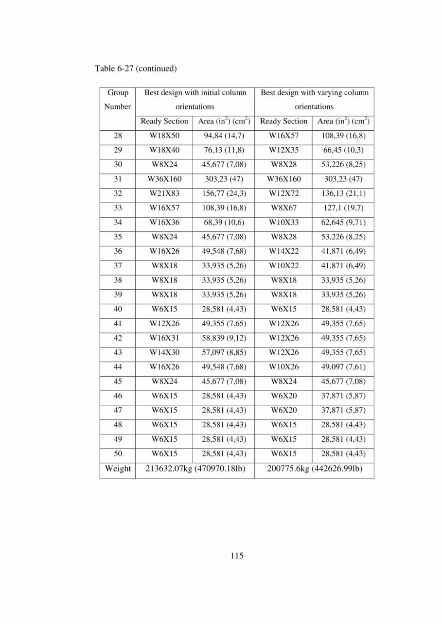
115



orientations


orientations

Group

Number

Ready Section Area (in2) (cm2) Ready Section Area (in2) (cm2)

28 W18X50 94,84 (14,7) W16X57 108,39 (16,8)

29 W18X40 76,13 (11,8) W12X35 66,45 (10,3)

30 W8X24 45,677 (7,08) W8X28 53,226 (8,25)

31 W36X160 303,23 (47) W36X160 303,23 (47)

32 W21X83 156,77 (24,3) W12X72 136,13 (21,1)

33 W16X57 108,39 (16,8) W8X67 127,1 (19,7)

34 W16X36 68,39 (10,6) W10X33 62,645 (9,71)

35 W8X24 45,677 (7,08) W8X28 53,226 (8,25)

36 W16X26 49,548 (7,68) W14X22 41,871 (6,49)

37 W8X18 33,935 (5,26) W10X22 41,871 (6,49)

38 W8X18 33,935 (5,26) W8X18 33,935 (5,26)

39 W8X18 33,935 (5,26) W8X18 33,935 (5,26)

40 W6X15 28,581 (4,43) W6X15 28,581 (4,43)

41 W12X26 49,355 (7,65) W12X26 49,355 (7,65)

42 W16X31 58,839 (9,12) W12X26 49,355 (7,65)

43 W14X30 57,097 (8,85) W12X26 49,355 (7,65)

44 W16X26 49,548 (7,68) W10X26 49,097 (7,61)

45 W8X24 45,677 (7,08) W8X24 45,677 (7,08)

46 W6X15 28,581 (4,43) W6X20 37,871 (5,87)

47 W6X15 28,581 (4,43) W6X20 37,871 (5,87)

48 W6X15 28,581 (4,43) W6X15 28,581 (4,43)

49 W6X15 28,581 (4,43) W6X15 28,581 (4,43)

50 W6X15 28,581 (4,43) W6X15 28,581 (4,43)

Weight 213632.07kg (470970.18lb) 200775.6kg (442626.99lb)

116

350000

450000

550000

650000

750000

850000

950000

1050000

1150000

1250000

50 100 200 400 600 800 900 950 1000


Bes

t Fea

sibe

Des

ign

Wei

ght

Test 1

Test 2

Test 3

Test 1

Test 2

Test 3

Test 4

Test 5





117



The fourth (last) design example is a braced space steel frame consisting of

1540 joints and 3590 members that are to be built in three adjacent blocks. The

3D, side and plan views of the frame at different story levels are shown in

Figure 6.22. The first, second and third blocks consist of 12, 18 and 30 stories

with an equal story height of 12ft. The bays are 24ft long in both directions. An

economical and effective stiffening of the frame against lateral forces is

achieved through exterior diagonal bracing members located on the perimeter

of the building as well as on the adjacent sides of the blocks. The diagonal

members are also known to participate in transmitting gravity forces. All the

columns are connected to the foundation with fixed connections.


collected under 129 member size groups; 104 column size groups, 20 beam

size groups and 5 bracing size groups. The member groups are clearly

tabulated in Table 6-28. The grouping of the members is performed both in

plan and elevation levels. A plan level grouping of columns is shown in Figure

6.23. The columns are collected in 16 size groups at each level between 1-12th

stories (Figure 6.23a), in 10 groups at each level between 13-18th stories

(Figure 6.23b), and in 4 groups at each level between 19-30th stories (Figure

6.23c). On the other hand, beams are collected under two groups as outer and

inner beams in plan level grouping. In elevation level grouping, the column

size groups are to have the same section over three adjacent stories, as are

beam size groups. Bracing members are designed as three-story deep members,

and a single bracing size group is specified in every six stories.

The orientation variables are assigned, keeping in mind that all the successive

columns along the frame height must have the same orientation. Hence, each

118

column group in Figure 6.23(a) is associated with an orientation variable,

resulting in sixteen orientation variables in all.

The frame is subjected to two loading conditions of combined gravity and wind

forces. Load cases and combinations are determined according to the ASCE 7-

05 [43], as explained in Section 6.2. Only the 1st and the 2nd combinations that

are tabulated in Table 6-2 are taken into consideration for this design example.

The resulting gravity loading on the beams of roof and floors is tabulated in

Table 6-29 and the wind loadings on windward and leeward faces of the frame


Table 6-30.


column members, while beams and diagonals are selected from discrete sets of

171 and 147 economical sections selected from wide-flange profile list based

on area and inertia properties in the former, and on area and radii of gyration

properties in the latter. Provisions of ASD-AISC [39] are taken into

consideration for the stress, stability, and geometric constraints. Displacements

of all the joints in x and y directions are limited to 27.43cm (10.8 in), and the

upper limit of inter story drifts is set to 0.91cm (0.36in), which is equal to the

story height/400.

Two design cases are studied. First, the structure is designed for minimum

weight considering the size design variables only, where initial orientations of

the column members are kept unchanged. Second, size and orientation

variables are employed together to minimize the weight of the frame.

119

(a) 3D view

120

(b) Plan view

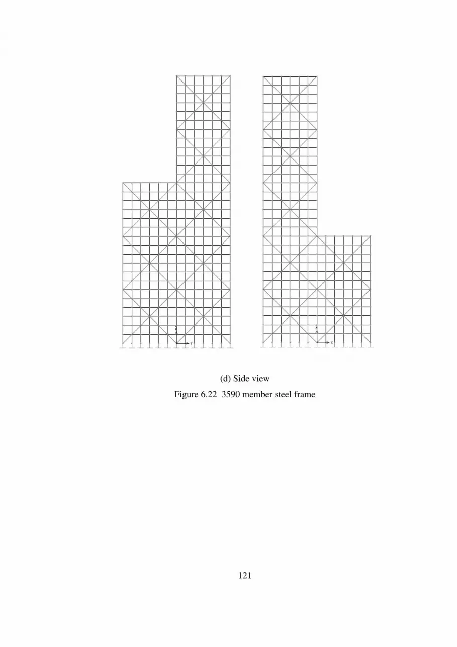
121

(d) Side view


122


123

Table 6-28 Member grouping for 3590-member steel frame

Member

Group Group Name

Member

Group Group Name

1st, 2nd and 3rd floors

1 Corner columns on axis A1 10 Corner columns on axis M1,

M7

2 Corner columns on axis A7 11 Outer columns on axis H-

L/1, H-L/7

3 Corner columns on axis G1 12 Outer columns on axis M/2-

6

4 Corner columns on axis G7 13 Inner columns on axis I/3-4,

K/3-4

5 Outer columns on axis B-F/1 14 Corner columns on axis A13

and G13

6 Outer columns on axis A/2-6 15 Outer columns on axis A/8-

12, G/8-12

7 Inner columns on axis B-F/7 16 Outer columns on axis B-

F/13

8 Inner columns on axis G/2-6 17 Inner columns on axis C/9-

11, E/9-11

9 Inner columns on axis C/3-4,

E/3-4

4th, 5th and 6th floors

18 Corner columns on axis A1

27

Corner columns on axis M1,

M7


28

Outer columns on axis H-

L/1, H-L/7

20 Corner columns on axis G1

29

Outer columns on axis M/2-

6


30

Inner columns on axis I/3-4,

K/3-4

22 Outer columns on axis B-F/1

31

Corner columns on axis A13

and G13

124


Member

Group Group Name

Member

Group Group Name

23 Outer columns on axis A/2-6

32

Outer columns on axis A/8-

12, G/8-12

24 Inner columns on axis B-F/7

33

Outer columns on axis B-

F/13

25 Inner columns on axis G/2-6

34

Inner columns on axis C/9-

11, E/9-11

26

Inner columns on axis C/3-4,

E/3-4



44


M7


45


L/1, H-L/7


46


6


47


K/3-4


48


and G13


49


12, G/8-12


50


F/13


51


11, E/9-11

43


E/3-4



61


M7


62


L/1, H-L/7

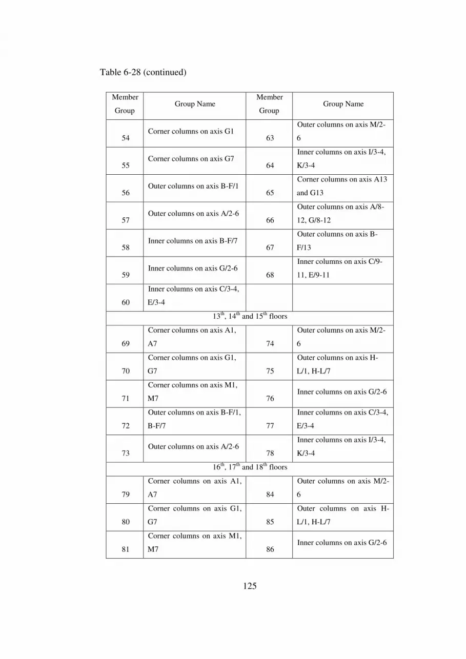
125


Member

Group Group Name

Member

Group Group Name


63


6


64


K/3-4


65


and G13


66


12, G/8-12


67


F/13


68


11, E/9-11

60


E/3-4


69

Corner columns on axis A1,

A7 74


6

70

Corner columns on axis G1,

G7 75


L/1, H-L/7

71


M7 76 Inner columns on axis G/2-6

72

Outer columns on axis B-F/1,

B-F/7 77


E/3-4


78


K/3-4


79


A7 84


6

80

Corner columns on axis G1,

G7 85


L/1, H-L/7

81


M7 86 Inner columns on axis G/2-6

126


Member

Group Group Name

Member

Group Group Name

82

Outer columns on axis B-F/1,

B-F/7 87


E/3-4


88


K/3-4

19th, 20th and 21st floors

89


A7, G1 and G7 91


F/1, B-F/7

90

Outer columns on axis A/2-6,

G/2-6 92


E/3-4

22nd, 23rd and 24th floors

93


A7, G1 and G7 95


F/1, B-F/7

94


G/2-6 96


E/3-4


97


A7, G1 and G7 99


F/1, B-F/7

98


G/2-6 100


E/3-4


101


A7, G1 and G7 103


F/1, B-F/7

102


G/2-6 104


E/3-4

Beams

105

Inner beams between 1-3

stories 115


stories

106

Outer beams between 1-3

stories 116


stories

107


stories 117


stories

127


Member

Group Group Name

Member

Group Group Name

108


stories 118


stories

109


stories 119


stories

110


stories 120


stories

111


stories 121


stories

112


stories 122


stories

113


stories 123


stories

114


stories 124


stories

Bracings

125 Bracings between 1-6 stories 128

Bracings between 19-24

stories

126


stories 129


stories

127


stories



Outer Beams Inner Beams

Beam Type

kN/m(lb/ft) kN/m(lb/ft)

Roof Beams 8.86 (607.04) 17.72 (1214.08)

Floor Beams 12.86 (881.04) 25.72 (1762.08)

(a) 24ft span

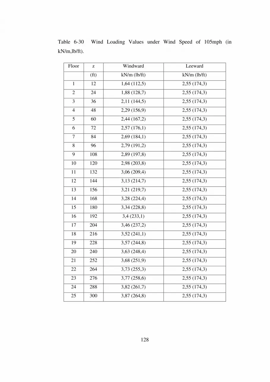
128

Table 6-30 Wind Loading Values under Wind Speed of 105mph (in

kN/m,lb/ft).



1 12 1,64 (112,5) 2,55 (174,3)

2 24 1,88 (128,7) 2,55 (174,3)

3 36 2,11 (144,5) 2,55 (174,3)

4 48 2,29 (156,9) 2,55 (174,3)

5 60 2,44 (167,2) 2,55 (174,3)

6 72 2,57 (176,1) 2,55 (174,3)

7 84 2,69 (184,1) 2,55 (174,3)

8 96 2,79 (191,2) 2,55 (174,3)

9 108 2,89 (197,8) 2,55 (174,3)

10 120 2,98 (203,8) 2,55 (174,3)

11 132 3,06 (209,4) 2,55 (174,3)

12 144 3,13 (214,7) 2,55 (174,3)

13 156 3,21 (219,7) 2,55 (174,3)

14 168 3,28 (224,4) 2,55 (174,3)

15 180 3,34 (228,8) 2,55 (174,3)

16 192 3,4 (233,1) 2,55 (174,3)

17 204 3,46 (237,2) 2,55 (174,3)

18 216 3,52 (241,1) 2,55 (174,3)

19 228 3,57 (244,8) 2,55 (174,3)

20 240 3,63 (248,4) 2,55 (174,3)

21 252 3,68 (251,9) 2,55 (174,3)

22 264 3,73 (255,3) 2,55 (174,3)

23 276 3,77 (258,6) 2,55 (174,3)

24 288 3,82 (261,7) 2,55 (174,3)

25 300 3,87 (264,8) 2,55 (174,3)

129




26 312 3,91 (267,8) 2,55 (174,3)

27 324 3,95 (270,7) 2,55 (174,3)

28 336 3,99 (273,5) 2,55 (174,3)

29 348 4,03 (276,3) 2,55 (174,3)

30 360 2,04 (139,5) 1,27 (87,17)

6.8.2 Test Results




Table 6-31 or Figure 6.24 that the best design weight of 5,250,665.2lb

(2,381,701.74kg) is obtained when the frame is sized for minimum weight

under initial choice of column orientations. When column orientations are

permitted to vary in the optimization process, the best design weight of the

frame has been improved to 5,040,628.16lb (2,286,428.94kg). The sectional

designations attained for member groups in both design cases are compared in

Table 6-32. The optimal layout of the column orientation achieved in the latter

case is shown in Figure 6.25. It follows that the optimal layout of column

orientations can lead to a reduction as much as 3.6 % in the frame weight.





Total

Weight 5312947,4 5365007,2 5250665,2 5040628,2 5041610,1 5063400,7 5148126,3 5167920,7

Total

Volume 18773666 18957622,6 18553587 17811407 17814876,6 17891875,3 18191259,1 18261203,9

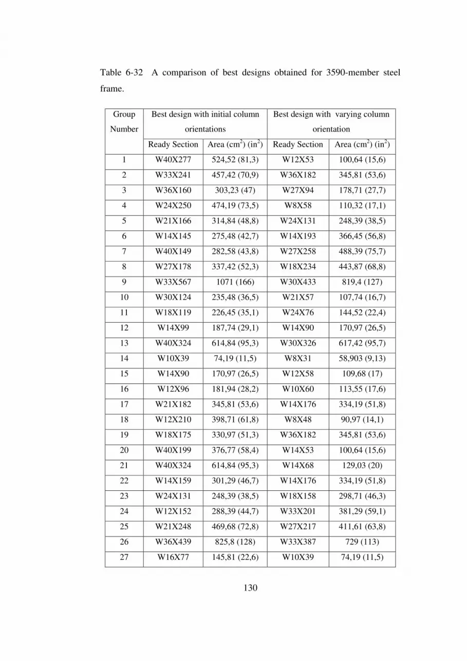
130


frame.


orientations


orientation

Group

Number

Ready Section Area (cm2) (in2) Ready Section Area (cm2) (in2)

1 W40X277 524,52 (81,3) W12X53 100,64 (15,6)

2 W33X241 457,42 (70,9) W36X182 345,81 (53,6)

3 W36X160 303,23 (47) W27X94 178,71 (27,7)

4 W24X250 474,19 (73,5) W8X58 110,32 (17,1)

5 W21X166 314,84 (48,8) W24X131 248,39 (38,5)

6 W14X145 275,48 (42,7) W14X193 366,45 (56,8)

7 W40X149 282,58 (43,8) W27X258 488,39 (75,7)

8 W27X178 337,42 (52,3) W18X234 443,87 (68,8)

9 W33X567 1071 (166) W30X433 819,4 (127)

10 W30X124 235,48 (36,5) W21X57 107,74 (16,7)

11 W18X119 226,45 (35,1) W24X76 144,52 (22,4)

12 W14X99 187,74 (29,1) W14X90 170,97 (26,5)

13 W40X324 614,84 (95,3) W30X326 617,42 (95,7)

14 W10X39 74,19 (11,5) W8X31 58,903 (9,13)

15 W14X90 170,97 (26,5) W12X58 109,68 (17)

16 W12X96 181,94 (28,2) W10X60 113,55 (17,6)

17 W21X182 345,81 (53,6) W14X176 334,19 (51,8)

18 W12X210 398,71 (61,8) W8X48 90,97 (14,1)

19 W18X175 330,97 (51,3) W36X182 345,81 (53,6)

20 W40X199 376,77 (58,4) W14X53 100,64 (15,6)

21 W40X324 614,84 (95,3) W14X68 129,03 (20)

22 W14X159 301,29 (46,7) W14X176 334,19 (51,8)

23 W24X131 248,39 (38,5) W18X158 298,71 (46,3)

24 W12X152 288,39 (44,7) W33X201 381,29 (59,1)

25 W21X248 469,68 (72,8) W27X217 411,61 (63,8)

26 W36X439 825,8 (128) W33X387 729 (113)

27 W16X77 145,81 (22,6) W10X39 74,19 (11,5)

131



orientations


orientation

Group

Number


28 W12X106 201,29 (31,2) W12X72 136,13 (21,1)

29 W21X101 192,26 (29,8) W18X97 183,87 (28,5)

30 W12X230 436,77 (67,7) W40X328 621,93 (96,4)

31 W21X44 83,87 (13) W10X30 57,032 (8,84)

32 W14X90 170,97 (26,5) W14X48 90,97 (14,1)

33 W14X99 187,74 (29,1) W12X45 85,16 (13,2)

34 W14X132 250,32 (38,8) W12X136 257,42 (39,9)

35 W36X135 256,13 (39,7) W14X99 187,74 (29,1)

36 W30X99 187,74 (29,1) W30X191 361,93 (56,1)

37 W18X40 76,13 (11,8) W14X34 64,52 (10)

38 W18X158 298,71 (46,3) W14X109 206,45 (32)

39 W18X143 271,61 (42,1) W30X124 235,48 (36,5)

40 W14X132 250,32 (38,8) W27X161 305,81 (47,4)

41 W27X146 276,77 (42,9) W14X159 301,29 (46,7)

42 W36X260 493,55 (76,5) W14X145 275,48 (42,7)

43 W30X526 993,5 (154) W27X368 696,8 (108)

44 W8X40 75,48 (11,7) W27X146 276,77 (42,9)

45 W14X109 206,45 (32) W16X77 145,81 (22,6)

46 W10X88 167,1 (25,9) W12X79 149,68 (23,2)

47 W24X229 433,55 (67,2) W36X245 465,16 (72,1)

48 W8X24 45,677 (7,08) W14X99 187,74 (29,1)

49 W12X106 201,29 (31,2) W14X48 90,97 (14,1)

50 W24X94 178,71 (27,7) W16X40 76,13 (11,8)

51 W21X111 210,97 (32,7) W14X90 170,97 (26,5)

52 W40X199 376,77 (58,4) W8X58 110,32 (17,1)

53 W21X83 156,77 (24,3) W33X141 268,39 (41,6)

54 W14X43 81,29 (12,6) W12X40 76,13 (11,8)

55 W16X77 145,81 (22,6) W27X94 178,71 (27,7)

132



orientations


orientation

Group

Number


56 W18X130 246,45 (38,2) W18X119 226,45 (35,1)

57 W10X100 189,68 (29,4) W27X102 193,55 (30)

58 W10X100 189,68 (29,4) W30X108 204,52 (31,7)

59 W40X192 364,52 (56,5) W40X215 408,39 (63,3)

60 W30X357 671 (104) W24X306 579,35 (89,8)

61 W6X20 37,871 (5,87) W14X38 72,26 (11,2)

62 W12X72 136,13 (21,1) W16X67 127,1 (19,7)

63 W10X68 129,03 (20) W10X88 167,1 (25,9)

64 W14X132 250,32 (38,8) W14X132 250,32 (38,8)

65 W8X15 28,645 (4,44) W6X16 30,581 (4,74)

66 W18X46 87,1 (13,5) W10X39 74,19 (11,5)

67 W24X84 159,35 (24,7) W10X39 74,19 (11,5)

68 W14X48 90,97 (14,1) W14X53 100,64 (15,6)

69 W14X99 187,74 (29,1) W30X108 204,52 (31,7)

70 W16X77 145,81 (22,6) W10X33 62,645 (9,71)

71 W12X106 201,29 (31,2) W27X94 178,71 (27,7)

72 W30X173 327,74 (50,8) W18X130 246,45 (38,2)

73 W36X182 345,81 (53,6) W27X161 305,81 (47,4)

74 W40X298 565,16 (87,6) W12X279 528,39 (81,9)

75 W14X61 115,48 (17,9) W14X26 49,613 (7,69)

76 W10X68 129,03 (20) W18X50 94,84 (14,7)

77 W12X79 149,68 (23,2) W10X77 145,81 (22,6)

78 W44X224 424,52 (65,8) W12X96 181,94 (28,2)

79 W12X58 109,68 (17) W30X173 327,74 (50,8)

80 W12X40 76,13 (11,8) W10X33 62,645 (9,71)

81 W18X130 246,45 (38,2) W30X99 187,74 (29,1)

82 W14X120 227,74 (35,3) W12X87 165,16 (25,6)

83 W36X135 256,13 (39,7) W40X167 316,77 (49,1)

133



orientations


orientation

Group

Number


84 W40X244 462,58 (71,7) W40X215 408,39 (63,3)

85 W5X19 35,742 (5,54) W10X22 41,871 (6,49)

86 W12X87 165,16 (25,6) W16X40 76,13 (11,8)

87 W21X101 192,26 (29,8) W12X72 136,13 (21,1)

88 W14X53 100,64 (15,6) W14X53 100,64 (15,6)

89 W12X40 76,13 (11,8) W14X53 100,64 (15,6)

90 W44X198 374,19 (58) W24X94 178,71 (27,7)

91 W18X106 200,64 (31,1) W27X84 160 (24,8)

92 W24X207 391,61 (60,7) W12X152 288,39 (44,7)

93 W18X35 66,45 (10,3) W16X36 68,39 (10,6)

94 W14X109 206,45 (32) W21X73 138,71 (21,5)

95 W10X100 189,68 (29,4) W16X67 127,1 (19,7)

96 W36X150 285,16 (44,2) W14X145 275,48 (42,7)

97 W16X67 127,1 (19,7) W21X111 210,97 (32,7)

98 W30X191 361,93 (56,1) W14X74 140,64 (21,8)

99 W21X68 129,03 (20) W24X62 117,42 (18,2)

100 W30X173 327,74 (50,8) W24X104 197,42 (30,6)

101 W18X55 104,52 (16,2) W10X15 28,452 (4,41)

102 W18X130 246,45 (38,2) W21X101 192,26 (29,8)

103 W10X112 212,26 (32,9) W36X135 256,13 (39,7)

104 W16X77 145,81 (22,6) W40X149 282,58 (43,8)

105 W21X44 83,87 (13) W18X35 66,45 (10,3)

106 W8X10 19,097 (2,96) W8X10 19,097 (2,96)

107 W18X35 66,45 (10,3) W18X35 66,45 (10,3)

108 W10X12 22,839 (3,54) W8X10 19,097 (2,96)

109 W18X35 66,45 (10,3) W21X50 94,84 (14,7)

110 W12X14 26,839 (4,16) W33X130 247,1 (38,3)

111 W21X44 83,87 (13) W24X55 104,52 (16,2)

134



orientations


orientation

Group

Number


112 W10X15 28,452 (4,41) W12X14 26,839 (4,16)

113 W21X83 156,77 (24,3) W16X45 85,81 (13,3)

114 W24X84 159,35 (24,7) W14X22 41,871 (6,49)

115 W16X40 76,13 (11,8) W16X40 76,13 (11,8)

116 W8X15 28,645 (4,44) W14X22 41,871 (6,49)

117 W16X40 76,13 (11,8) W18X46 87,1 (13,5)

118 W16X45 85,81 (13,3) W10X17 32,193 (4,99)

119 W18X50 94,84 (14,7) W18X50 94,84 (14,7)

120 W6X15 28,581 (4,43) W12X16 30,387 (4,71)

121 W33X118 223,87 (34,7) W24X55 104,52 (16,2)

122 W12X26 49,355 (7,65) W33X118 223,87 (34,7)

123 W24X55 104,52 (16,2) W33X130 247,1 (38,3)

124 W24X55 104,52 (16,2) W12X14 26,839 (4,16)

125 W14X233 441,93 (68,5) W40X298 565,16 (87,6)

126 W14X283 537,42 (83,3) W14X233 441,93 (68,5)

127 W14X257 487,74 (75,6) W14X233 441,93 (68,5)

128 W14X159 301,29 (46,7) W14X176 334,19 (51,8)

129 W14X90 170,97 (26,5) W14X109 206,45 (32)

Weight 2381701.735kg (5250665.2lb) 2,286,428.94kg(5,040,628.16lb)

135

4000000

5000000

6000000

7000000

8000000

9000000

10000000

11000000

12000000

50 100 200 400 600 800 900 950 1000


Bes

t F

easi

be

Des

ign

Wei

gh

t (l

b)

Test 1

Test 2

Test 3

Test 1

Test 2

Test 3

Test 4

Test 5




136


137

6.9 RESULTS AND EVALUATION

Four different problems are handled in the scope of this study. Each of the

structures is subjected to both gravity and lateral loads. For all of the structures,

wind load is applied as the lateral loads. The members of the structures are

grouped according to the aforementioned criterion. Each of the systems is

designed under two main conditions. In the first case only size variables are

taken into consideration and optimum weights are obtained according to the

initially chosen column orientations. For the second group of runs, orientation

variables are also taken as design variables.

For 960 member steel frame example, different wind loads are applied to the

same structure. The results revealed that an optimal orientation of the columns

results in structural designs which are about 4% to 8.5% lighter than the

designs that are based on initial column orientations chosen. 568 member steel

frame is analyzed for two different design cases. For the first design case,

inclusion of orientation variables results in a reduced structural weight which is

4.1% lighter than the case where members are only sized without a change in

their orientations. For the second design case, a reduction of 3.0% in the weight

of the structure is achieved by changing the orientations of the members. The

results of the two design cases are also differentiate in orientation of columns.

As the torsional moments are included, the orientations of the columns are

changed in a manner to satisfy the maximum torsional stiffness in the direction

of the moment. Figure 6.16. Similarly, for 1230 member steel frame example,

the optimal layout of column orientations leads to a reduction as much as 6.0 %

in the frames’ weights. For the last design example, 3590 member steel frame,

a 3.6% reduction in structural weight has been achieved with the proper

orientations of the columns. In general, for all of the design examples

considered in the study, a weight reduction between 4 % to 8 % has been

achieved when orientations of the columns are optimized during the design

process.

138

The column orientations can be predicted according to some design heuristics.

If the plan of the structure is square or almost square the system needs to have

same rigidity against both directions. This can be satisfied with column

orientations. The number of columns whose strong axes are in the same

direction with x axis of the structure should be equal to the one’s that are in y

direction. By this way the building’s resistance to the lateral loads will be

similar in both directions. In the 960 member steel frame structure, for all of

the different wind loads, 4 of the 7 column groups are placed in one direction

while the remaining ones are oriented in opposite direction (Figure 6.5, Figure

6.7 and Figure 6.10). There is a similar tendency in the 568 member steel

frame structure. For the first three floors, there are totally 7 column groups and

the strong axes of 4 of the columns are placed perpendicular to x direction

while the 3 of them are oriented in the other direction (Figure 6.14, Figure

6.16). The orientations of the columns in the first three floors are also the same

in the upper parts of the structure since all the successive columns along the

frame height must have the same orientations. This results with a 2 groups of

columns that are orientated in local 3-3 direction and 2 of them that are

orientated in local 2-2 direction. In case of a rectangular building, columns are

placed with their strong axis perpendicular to short side in order to increase

resistance of the building against bending along short side. The columns are

placed with their strong axis perpendicular to short side. 1230 member steel

frame structure is an example for the tendency of the column orientation in a

rectangular building (Figure 6.21). However, as for the non-symmetrical

structures such as 3590 member steel frame structure, a generalization is hard

to do; the optimization program chooses the most appropriate orientation of

each column according to the behavior of the structure. Intuition of the

designer might not be enough to place the columns in the correct orientation.

Column orientations of the symmetrical systems that are square in plan view

show a similarity in the investigated problems. In both of the directions, outer

columns of the frames are oriented on their strong axis on the frame direction

139

(Figure 6.5, Figure 6.7, Figure 6.10, Figure 6.14). There is an exception about

the corner columns. The orientation of inner columns differs in order to satisfy

similar stiffness in both of the directions. There is logic behind this orientation.

This can be explained basically by the cantilever method. Under the effect of

lateral loads, the structure behaves like a cantilever and the outer columns

resist to tension and compression forces Figure 6.26, Figure 6.27. This means

that most of the axial forces are taken by the outer columns. The moment that

results from the lateral loads are shared according to the stiffness of the

columns Figure 6.26, Figure 6.27. It is already mentioned that the stress on the

frame is the combination of the ratio of axial force to section area and the ratio

of moments to section modulus Equation ( 4.3). It is reasonable to rotate the

outer columns on their strong axis. This will help to decrease the total stress on

the member by strengthening the section modulus of the member. The profile

that is assigned to the member will be used efficiently with correct orientation.

Figure 6.26 Lateral loading of a general steel frame

140

(a) Axial Force Diagram

(b) Moment Diagram

Figure 6.27 Behavior of a frame under lateral loading

141

CHAPTER 7

CONCLUSION

7.1 CONCLUSIONS AND SUGGESTIONS

The optimum design process of the steel frames in the literature is only based

on sizing of structural members in which orientations of the columns are

determined initially and kept constant during optimum design process. In this

study, the effect of the appropriate choice of column orientation on minimum

weight design of steel frames is investigated. Evolution strategies is used as a

tool for sizing optimization of the steel structures. In addition, size

optimization is integrated with orientation optimization to further reduce the

weight of the structures under certain restrictions and constraints imposed by

design specifications. Each of the systems is designed under two main

conditions. In the first case only size variables are taken into consideration and

optimum weights are obtained according to the initially chosen column

orientations. For the second group of runs, orientation variables are also taken

as design variables.

The results revealed that an optimal orientation of the columns results in

structural designs which are about 4% to 8% lighter than the designs that are

based on initial column orientations chosen.

Design heuristics may be in benefit of the designer while defining the initial

column orientations of the structures. In case of a structure that’s plan view is

square or almost square the system needs to have same rigidity against both

directions. Equivalent rigidity in both of the directions can be satisfied with

column orientations. The number of columns whose strong axes are in the

same direction with x axis of the structure should be equal to the one’s that are

142

in y direction. The resistance of the structure to lateral loads in both directions

will be similar with this orientation. If the plan view of the system is

rectangular, the columns are placed with their strong axis perpendicular to

short side. By this way the resistance of the building is increased against

bending along short side. A generalization is hard to do for non-symmetrical

structures. The appropriate column orientation of the structure is assigned by

the program according to the behavior of the structure. Intuition of the designer

might not be enough to place the columns in the correct orientation.

A similarity is revealed for the investigated problems on column orientations.

For the symmetrical systems the outer columns are orientated in the same way.

The outer columns of the structure are oriented on their strong axis on the

frame direction. However, as for the corner columns a generalization is hard to

do. The inner corner columns are oriented in both of the directions to satisfy

similar stiffness in both of the directions.

7.2 RECOMMANDATIONS FOR FUTURE STUDIES

The following related subjects shall be investigated in the future studies:

• The effect of column orientation to optimization in industrial structures.

• The effect of column orientation to optimization with additional design

provisions like TEC-07.

• The effect of inclusion of geometric constraints to structural

optimization.

• The design heuristics of column orientations of non-symmetrical

structures.

• Performance of other metaheuristic search techniques with the inclusion

of orientation variables to design variables.

143

REFERENCES

[1] O. Hasançebi, S. Carbaş, E. Doğan, F. Erdal and M.P. Saka, Performance

evaluation of metaheuristic search techniques in the optimum design of

real size pin jointed structures, Computers and Structures 87 (5–6)

(2009), pp. 284–302.

[2] Papadrakakis, M., Lagaros, N., Tsompanakis, Y., Structural optimization

using evolution strategies and neural networks. In: Fourth U.S. National

Congress on Computational Mechanics, San Francisco (1997)

[3] Spallino, S. and Rizzo, S., Multi-objective discrete optimization of

laminated structures, Mech Res Commun 29 (2002), pp. 17–25.

[4] Pareto, V., Cours d’Economie Politique. F. Rouge, Lausanne, 1896

[5] Gutkowski, W., Iwanow, Z. and Bauer, J., Controlled mutation in

evolutionary structural optimization. Struct. Multidisc. Optim 21 (2001),

pp. 355–360.

[6] Lagaros, N.D., Papadrakakis, M., and Kokossalakis, G., Structural

optimization using evolutionary algorithms. Comput. Struct. 80 7–8

(2002), pp. 571–589.

[7] Ebenau, C., Rottschäfer, J., and Thierauf, G., An advanced evolution

strategy with an adaptive penalty function for mixed-discrete structural

optimization. Adv. Eng. Software, 2005, 36(1) 29-38

[8] Lagaros, N.D., Charmpis, D.C., Papadrakakis, M., An adaptive neural

network strategy for improving the computational performance of

evolutionary structural optimization. Computer Methods in Applied

Mechanics and Engineering 2005; 194(30–33):3374–3393.

[9] Rajasekaran, S., Shalu, Mohan, V., Khamis, O., (2004) The optimization

of space structures using evolution strategies with functional networks.

Eng Comput. 20:75–87

144

[10] Rajasekaran S., Mohan V.S. and Khamis O. (2004) “ The optimization of

space structures using evolution strategies with functional networks.”

Eng Comput 20 75-87

[11] Baumann, B. and Kost, B., Structure assembling by stochastic

optimization, Comput Struct 83 (2005), pp. 2175–2184.

[12] Holland, J. H. Adaptation in natural and artificial systems. Ann Arbor,

MI: The University of Michigan Press, 1975.

[13] Rechenberg I., Cybernetic Solution Path of an Experimental Problem.

Royal Aircraft Establishment, Farnborough, UK, Library translation

No.1122, 1965.

[14] Rechenberg I., Evolutionsstrategie: Optimierung technischer Systeme

nach Prinzipien der biologischen Evolution, 1973 (Fromman-Holzboog,

Stuttgart)

[15] Schwefel. H-P., Kybernetische Evolution als Strategie der

experimentellen Forschung in der Strömungtechnik, Diplomarbeit,

Technische Universität Berlin, 1965

[16] Fogel LJ, Owens AJ, Walsh MJ. Artificial intelligence through simulated

evolution. New York: Wiley, 1966.

[17] Kirkpatrick, S., Gerlatt, C.D., Vecchi, M.P., Optimization by simulated

annealing. Science 1983;220:671-80

[18] Kennedy, J., Eberhart, R., Particle swarm optimization. In:IEEE

international conference on neural networks, vol. 4. IEEE Press; 1995. p.

1942-8

[19] Xiaohui Hu, Particle swarm optimization,

http://www.swarmintelligence.org/tutorials.php, last accessed:

30.08.2009

[20] Glover, F., Tabu search-part I. ORSA J Comput 1989;1(3):190-206

[21] Fred Glover , Fred Laguna, Tabu Search, Kluwer Academic Publishers,

Norwell, MA, 1997

[22] Ülker, Ö., Özcan, E., 2006, Evolutionary tabu search algorithm for graph

coloring problem,

145

http://cse.yeditepe.edu.tr/~eozcan/research/papers/TBD20_1.pdf, last

accessed: 25.09.2009

[23] Dorigo., M., Stützle, T., Ant colony optimization a Bradford book. USA:

Massachusetts Institute of Technology; 2004

[24] Lee, K.S., Geem, Z.W., A new structural optimization method based on

the harmony search algorithm. Comput. Struct. 2004;82:781-98

[25] Geem, Z.W., Kim, J.-H., and Loganathan, G.V., A new heuristic

optimization algorithm: harmony search, Simulation 76 (2001), pp. 60–

68.

[26] Cai, J. and Thierauf, G. Discrete structural optimization using evolution

strategies. In Neural Networks and Combinatorial Optimization in Civil

and Structural Engineering. Topping B.H.V and Khan A.I.(eds) Civil-

Comp Limited Edinburgh, 1993

[27] Bäck T. and Schütz M. Evolution strategies for mixed-integer

optimization of optical multilayer systems. Proc of the 4th Annual Conf

on Evolutionary Programming. McDonnel J.R. Reynolds R.G and Fogel.

DB (eds.). MIT Press, Cambridge MA 33-51, 1995

[28] Rudolph, G., An evolutionary algorithm for integer programming, PPSN

III International Conference on Evolutionary Computation. In: Parallel

problem solving from nature. Lect. Notes Comput. Sci, vol. 866. Berlin:

Springer; 1994. p. 139-48.

[29] Klockgether J. and Schwefel H.-P Two-phase nozzle and hollow core jet

experiments. In Elliot D. (ed) Parallel Computing and Mathematical

Optimization, vol. 367 of Lecture Notes in Economics and Mathematical

Systems, pages 177-198. Springer, Berlin, March 1970

[30] Eiben, A.E., and Smith, J.E., Introduction to Evolutionary Computing.

Springer, 2003.

[31] Bäck, T. and Schwefel, H.-P., Evolution Strategies I: variants and their

computational implementation. In Genetic Algorithms in Engineering

and Computer Science, edited by G. Winter et al. pp.111-126,1995

(Wiley: Chichester).

146

[32] Schwefel H–P. Numerical optimization of computer models. Chichester:

Wiley, 1981.

[33] Bäck, T. and Schwefel, H.-P., An overview of evolutionary algorithms

for parameter optimization. Evolution. Comput., 1993, 1(1), 1-23

[34] Cai J and Thierauf G (2005) “Evolution strategies for solving discrete

optimization problems”, Adv Eng. Softw. 2 177-183

[35] Papadrakis and Lagaros (1998) Advanced solution methods in structural

optimization based on evolution strategies” Eng Comput 15 12-34

[36] Lagaros N.D. , Papadrakis M. and Kokossalakis G. (2002) “Structural

optimization using evolutionary algorithms.” Comput Struct.

[37] Papadrakis, M., Lagaros, N.D., and Fragakis, Y., Parallel computational

strategies for structural optimization. Int. J Num. Meth Eng., 2003 58(9),

1347-1380

[38] Hasançebi, O., Discrete approaches in evolution strategies based

optimum design of steel frames. Struct Eng Mech 2007; 26(2): 191-210.

[39] AISC, Manual of Steel Construction, Allowable Stress Design, 8th

edition, 1989 (American Institutes of Steel Construction: Chicago, IL)

[40] Dumonteil, P., “Simple Equations for Effective Length Factors”,

Engineering Journal, AISC, 29 (3), 111-115, 1992

[41] Hellesland, J., “Review and Evaluation of Effective Length Formulas”,

Research Report, No 94-2, University of Oslo, 1994

[42] Hasançebi. O., Adaptive evolution strategies in structural optimization:

enhancing their computational performance with applications to large-

scale structures. Comput, Struct. 2008;86(1-2):119-32

[43] ASCE 7-05, “Minimum Design Loads for Buildings and Other

Structures”, Published by American Society of Civil Engineers,1801

Alexander Bell Drive Reston, Virginia 20191