Download pdf - Models of central capacity and concurrency

JOURNAL OF MATHEMATICAL PSYCHOLOGY 28, 223-281 (1984)

Models of Central Capacity and Concurrency

RICHARD SCHWEICKERT

Purdue University

AND

GEORGE J. BOGGS

GTE Laboratories Incorporated

According to single channel theory, the ability of humans to perform concurrent mental operations is limited by the capacity of a central mechanism. The theory was developed by analogy with early computers which had a single central processing unit and required sequential processing. These limitations are not likely to be properties of the mind. But now computers have begun to employ extensive concurrent processing, because of the decreasing cost of the necessary hardware. In this review we will try to bring the computer analogy up to date. Theoretical issues important for concurrent systems may be of interest to psychologists and have applications to such problems as the speed-accuracy trade-off. Several hypotheses about the way signals gain access to the central mechanism are reviewed. Recent variations of the single channel theory are discussed, including the hypotheses that more than one process can use the central mechanism at a time, and that some processes do not use the central mechanism and can be executed concurrently with those that do. In addition, relevant concepts from scheduling theory and operating systems theory are introduced and difficulties encountered by concurrent systems, namely complexity, deadlocks, and thrashing, are discussed. 0 1984 Academic Prem, Inc.

CONTENTS. Introduction. 1. Single channel theory. 1.1. Access to the single channel. 1.2. Scheduling processes in the single channel. 1.3. Evidence against completely serial models. 2. Concurrent processes in the central mechanism. 2.1. Concurrency with variable capacity. 2.2. Concurrency with fixed capacity. 2.3. Concurrency and capacity in general. 3. Concurrent processes outside the central mechanism. 3.1. The organization of processes. 3.2. The nature of central processes. 3.3. The nature of noncentral processes. 3.4. Scheduling theory. 4. Conclusion. Appendix: Glossary.

The four most fundamental variables in cognitive psychology are probably information, utility, time, and capacity. Procedures for measuring the first three variables

Reprint requests should be addressed to Richard Schweickert, Department of Psychdogical Sciences, Purdue University, Peirce Hall, West Lafayette, Indiana 47907.

223 0022-2496184 83.00

Copyright 8 1984 by Academic Press, Inc. All rights of reproduction in any form reserved.

224 SCHWEICKERT AND BOGGS

have been developed, but several difftculties have prevented clear agreement about measuring capacity. First, there are many kinds of resources, such as memories, mechanisms, switches, and channels, and a different notion of capacity may be required for each. We do not know how many of these resources there are, or even if they are separate entities. We do not know, for example, whether there are one, two, or many types of memories. Second, resources are probably used in combination, but we do not know how the capacity of a combination of resources is related to their individual capacities. Finally, a natural variable for measuring capacity is the percent of responses which are correct. At the moment, we usually treat percent correct as a one dimensional ordinal variable, and this treatment is too improverished for the complicated structures we are attempting to measure.

We have decided to review the theories of central capacity and concurrency because these theories have become more sophisticated and testable as the experimental findings have become more intricate and robust. Furthermore, there has been a recent surge of relevant theoretical activity on these topics in computer science, due in part to advances in hardware making massive concurrent processing possible. Contemporary understanding of the mind is based largely on an analogy with the computer. The architecture of computers has changed considerably since the comparison was first made and one of the purposes of this review is to bring the analogy up to date.

Scope of the Review. Any review must leave out certain topics which are important, but not part of the subject at hand. This will be a review of theoretical ideas and not of experimental findings, except as needed to explain aspects of the theories. Reviews of the phenomena described by these theories are given by Bertleson (1966), Kantowitz (1974), Kerr (1973), and Smith (1967). We will discuss the concept of capacity only for concurrent processing because there are already two papers devoted to the general issue of capacity, a critique of the concepts and logic by Kantowitz (1984), and a critique of the methodologies by Duncan (1980). Finally, while there are many hypotheses about capacity in peripheral processing (e.g., Estes, 1972), our review will mainly concern central processing, and only occasionally sensory or response processing.

We will begin by discussing the single channel theory and how certain simple versions of it have failed, those which proposed that only one mental process is executed at a time. Then current more successful versions of the theory will be discussed, and some general notions of capacity will be introduced. We will then introduce some ideas about concurrent processing from scheduling theory. As we go along, we will present several issues which arise in scheduling theory and the design of operating systems which are potentially important for understanding concurrent mental processing.

Unfortunately, we have not been able to knit all the loose ends together into a unified theory. There are many ways the human information processing system could work, and it sometimes seems that every variation has been proposed at one time or another. The problem is not to create yet another model, but to eliminate some of

CAPACITY AND CONCURRENCY 225

those already existing. Most attempts to define the single channel theory to make it fit the facts have yielded post hoc models not testable by the available data. We will point out when we can that a certain form of a model is impossible, but the possibilities which remain are many.

1. SINGLE CHANNEL THEORY

In 1931 Telford reported that if one stimulus is followed closely by another, the time to respond to the second one is longer than if it were presented alone. Drawing an analogy with cardiac and neural tissue, he said the delay was due to a refractory period of decreased excitability in the attention system following a voluntary response. The term “psychological refractory period” has remained as a label for the phenomenon, although the neural analogy is no longer seen as suitable, because, for one thing, the period is not of fixed duration, as it is for neurons.

A more powerful analogy was used by Craik to explain the results of tracking experiments done during World War II (Craik, 1947, 1948; Vince 1948). He found that humans make intermittent, rather than continuous corrections while tracking. He said that the nervous system may be regarded as containing a “computing system”, perhaps in the cortex of the brain. Corrections occur only intermittently because “new sensory impulses entering the brain while this central computing process was going on would either disturb it or be hindered from disturbing it by some ‘switching’ system” (Craik, 1947, p. 147). Support for the idea that the origin of the psychological refractory period was central, rather than peripheral, was provided by Davis (1957), who showed that such a delay occurs when two stimuli are presented to different modalities.

Craik’s ideas were extended by Welford (1952, 1959, 1967, 1980) who said the central processes, or more specifically, the decisions, about two separate stimuli cannot overlap in time. If two stimuli arrive close together, one must be held in storage while the central mechanism is occupied by the other. To quantify these ideas, an estimate of the central processing time is desirable. Hick and Welford (1956) said that due to the limited capacity of the central mechanism, the central time for a stimulus increases as the information in the stimulus increases, in accordance with Hick’s law (Hick, 1952). But the central time is not observable directly, and so Welford used the entire reaction time for the first stimulus RT, as an approximation to its central processing time. Let I be the time interval between the two stimuli. The reaction time for the second stimulus RT, would be the waiting time until the central processing of the first stimulus is finished, RT, -1, plus the time which would be required to respond to the second stimulus if it were presented alone, RT,, (see Fig. 1). Then,

assuming I < RT, .

RT,=RT,,+RT,-I, (1)


RTI --I-. RT,-I-, RT”

52. RT2 f2 T

FIG. 1. Stimulus si is followed after an interval I by stimulus sI. The diagram shows the calculation of the reaction time to s2, RT,, if processing s2 does not start until the response to s, is made at I,.

There is often a delay in the response to the second stimulus even when it is presented after the response to the first stimulus has been made. The equation above does not predict this delay, but Welford’s theory can be extended to accomodate it by saying that if feedback from the first response reaches the central mechanism before the second stimulus does, then processing the feedback will occupy the mechanism, while the second stimulus must wait.

More complicated single channel models were developed by analogy with the von Neuman model for constructing computers, which was, in turn, influenced by ideas from psychology (von Neuman, 1958). In the von Neuman model, a computer has several peripheral devices accepting inputs, which are sent to a central processing unit, operating on one task at a time. Outputs are sent to peripheral devices, which might process several tasks simultaneously. The amount of information which can be sent through a channel in a computer is specified in the channel capacity theorem of information theory (Shannon dc Weaver, 1949).

The first to incorporate these ideas in a complete psychological theory was Broadbent (1958, 1971). A schematic representation of his model is given in Fig. 2. In the model, early stages of the nervous system can pass information simultaneously, but there is a later channel which cannot process more than a limited amount of information during a given time. In principle, the limited capacity channel can process more than one message at a time, as long as the combined information does not exceed the capacity (Broadbent, 1958, p. 298). The limited capacity channel is preceded by a filter which selects information from sensory inputs having some features in common. Additional bases for selection were included in the 1971 model. i As in Welford’s model, incoming information may be held in a short term store which precedes the channel if the channel is busy. If the stored information does not decay, which would occur within a few seconds, it may be selected as input to the channel. To avoid decay, information may be sent through the channel, and then fed back to the short term store, or, in the 1971 model, perhaps to a different store. Long term storage of the conditional probabilities of past events only takes place for those events which have passed through the limited capacity channel. The 1958 and 1971 models are quite similar, and the differences are listed in Broadbent’s 1971 book.

’ Two points should be noted: First, filtering is optional (not obligatory), and second, simultaneous channels exist for postfiltered stimuli as well as pretiltered stimuli (D. E. Broadbent, personal communication, December 1, 1981).


PROBABIL OF PAST EVENTS

LIMITED CAPACITY (P SYSTEM)

CHANNEL

SYSTEM FOR VARYING OUTPUT UNTIL SOME INPUT IS SELECTED

FIG. 2. Broadbent’s model of the human information processing system.

1.1. Access to the Single Channel

Broadbent’s theory was developed to explain, among other things, the results of dichotic listening experiments. In these expreiments, a subject is presented with two different messages, one to each ear (Broadbent, 1952; Cherry, 1953). His task is to recite, or “shadow” one of the messages as it goes along. Usually the subject can remember little about the unshadowed message afterwards; he is often unable to tell, for instance, whether the language of the rejected message was entirely English.

Alterations to Broadbent’s model have been suggested to make it consistent with later findings in dichotic listening experiments. One finding, for example, is that important words in the unshadowed message, such as the subject’s name, can be recalled later (Moray, 1959). This is not possible with Broadbent’s 1958 model, in which rejected information does not reach the limited channel at all, and hence is not stored in the long term store. At what point in the system is information destined for the single channel selected? Virtually every possibility has been suggested: early in processing, in the middle, towards the end, and the ultimate suggestion, prior to processing, based on feedback from the preceding signal.

Moray (1970) proposed an early selection model which incorporates a number of sensory channels which are available by means of a “switch” to a limited capacity single channel, which leads to a central processor. The following assumptions were made (a) at any moment, an observer is sampling only one message, via the single channel, and all others are totally rejected; (b) a running level is kept of activity within each sensory channel; (c) a sudden deviation in activity from the running level of a sensory channel will elicit a switch to sample that sensory channel; and (d) sampling may be continued in one sensory channel unless a deviation in the level of another sensory channel requires switching.

In the models of Broadbent and Moray, selection is based on elementary features of the stimuli and occurs before information reaches the central processor. Treisman


(1964, 1969) devised a model permitting selection based on deeper analysis, occuring in any of several stages of processing. A series of tests is performed on incoming messages and if an unwanted message can be distinguished on the basis of critical features, it is attenuated. This feature analysis can occur concurrently for inputs from different sensory channels. If no readily distinguishable features are available, “selection between messages... takes place during, rather than before or after, the analysis which results in the identification of their verbal context. It seems to be at this stage that the information-handling capacity becomes limited and can handle only one input at a time” (Treisman, 1964, p. 216).

A model by Deutsch and Deutsch (1963) places the selection process relatively late in the system. They propose that the processing system performs a sufficiently complete analysis of incoming information so that signals can be ordered in “importance.” A bottleneck occurs at the central processor, where all signals are compared for importance, and only those which meet or surpass some criterion of importance are acted upon.

The problem these models address is to account for selection into the single channel, when the basis for selection seems to be so complicated that only the single channel is capable of doing it. A way out of the dilemma is suggested by Norman (1968). In his model, early sensory analysis is done without recourse to the central processor. All sensory inputs, attended to or not, activate their representations in memory. Meanwhile, memory representations of various entities, some corresponding to present sensory inputs, some not, are activated because of their pertinence. The level of pertinence is determined by context, grammar, and other cues, supplied in part by previous outputs of the central processor. Those items which have a high combined activation in memory from both pertinence and sensory input are selected for further processing in the single channel.

Support for Norman’s model comes not only from dichotic listening experiments, but from two other phenomena, (a) sequential effects-in choice reaction time tasks, subjects are quick to identify an item if it was presented recently (Kornblum, 1973), and (b) priming effects-in lexical decision tasks, subjects are quick to decide a string is a word if a related word was presented recently (Meyer, Schvaneveldt, & Ruddy, 1975; Neely, 1977).

With Norman’s model, we come full circle. Broadbent and Moray suggested that selection occurs prior to central processing and is based on a simple analysis of the signals. In Deutsch and Deutsch’s model (1963), selection occurs during central processing itself. Treisman allows both possibilities. Norman’s model returns to the idea that selection precedes central processing, but the basis for selection is acknowledged to be so complicated that only the single channel is capable of doing it. To avoid a logical impossibility, the basis is determined not by the items currently waiting to enter the channel, but by those just finished with the single channel. We will see below that there is a useful function which could be served by activating memories associated with the current item in accordance with Norman’s model, namely the avoidance of thrashing.

The data on the locus of selection have been ambiguous, and neither early- nor


late-selection models can be firmly rejected. A good review of the current state can be found in Miller (1982a). He describes nice theoretical predictions of two types of models that may permit an empirical distinction. His reasoning is that late-selection models, in general, predict different cumulative distribution functions for reaction time than early-selection models (pp. 253-254). Miller’s data favor late-selection over early-selection models.

1.2. Scheduling Proctyses in the Single Channel

Let us postulate for the moment the existence of a central mechanism which can execute only one process at a time. Suppose a set of processes X, ,..., x, are somehow selected to use the central mechanism and arrive at the same time. In what order should they use it? The answer depends, of course, on what the subject is trying to optimize. If a single response is made after all the processes are executed, then the order is irrelevant. But if the completion time of each process is important, perhaps because a response is made after each process is completed, then the execution order will make a difference.

The quantity to be optimized can often be defined in terms of the following quantities. Let ti, a fixed quantity, be the duration of process xi. Let wi, the waiting time for process xi, be the amount of time elapsing from when xi arrives at the central mechanism until xl begins execution. Theflow time fr for process xi is the total time from its arrival until its completion, fr = w, + t,.

If there is a deadline for process xi. let di be the time at which xi is to be completed. The lateness of process xi is L, =A - di ; note that if xi is completed early this quantity is negative. The tardiness of process xi is max{O, Li}, a nonnegative quantity.

Several quantities are optimized by scheduling in the order of nondecreasing processing time, that is, executing xi before xi if ti < tj. This “shortest processing time first” procedure can be shown (Conway, Maxwell, & Miller, 1967) to minimize the mean flow time, the mean waiting time, and the mean lateness. This procedure also minimizes the average number of processes in the system which are either executing or waiting.

Another useful procedure schedules the processes in order of nondecreasing deadlines. That is, xi is executed before xi if the deadline for xi is earlier than the deadline for xj. It can be shown (Conway, Maxwell & Miller, 1967) that this procedure will minimize the maximum lateness and the maximum tardiness. The usefulness of these results is that they suggest that the subject could be induced to change his scheduling strategy in a predictable way depending on the payoffs arranged by the experimenter.

1.2.2. Timesharing

We assumed above that once a process begins execution it is not interrupted. But there are advantages to a system which allows preemptive timesharing, that is, interrupting one process to work on another and returning to the first one later. One


problem preemption could solve is that processes requiring the central mechanism may not all arrive at the same time. If interruption is allowed, it can be shown that at any given time the process which has the shortest remaining processing time should be selected for execution, provided there is no cost for interrupting the process currently being executed. This procedure will minimize the mean flow time, mean waiting time, mean lateness, and the inventory of processes waiting or in execution (Conway, Maxwell & Miller, 1967). Another problem which can be handled by preemptive timesharing is that the processing times may not be known ahead of time for processes arriving at the central mechanism. If preemption is allowed, each process in turn can be given a short burst of time, and in this way the ones with the shortest processing time will automatically be completed tirst.

Tolkmitt (1973) proposed a timesharing model with three major assumptions, which we will briefly summarize. First, mental processes, except peripheral ones, require the central mechanism, and processing in the mechanism is strictly sequential. Second, central processing times are additive, that is, the combined processing time of several processes, each of which uses the central mechanism, is the sum of the processing times of the individual processes. Third, “processing in the single channel can be temporarily interrupted” (Tolkmitt, 1973, p. 150).

One of the phenomena which Tolkmitt’s hypothesis explains is that the amount of time required to respond to one of two stimuli presented close together in time can be affected by the complexity of either stimulus. Tolkmitt explains this by saying that the central mechanism begins processing the first stimulus, but is interrupted temporarily when the second stimulus arrives. More time is required to interrupt a process, save preliminary results, start another process, and then resume the first process if one or the other or both of the processes are more complex. It is of great theoretical interest to know whether such preemptive processing takes place, but at the moment no experimental procedure is available to answer this question, because it would be difficult experimentally to distinguish timesharing from another kind of processing we discuss later, multiprocessing.

1.2.2. Thrashing

Early versions of timesharing computer systems suffered from an unforseen problem-if more than a few programs were loaded into the system, progress would slow to a halt, although in principle there were enough memory locations and processors to handle the load. Almost all the capacity of the system was being employed to search for empty memory locations in which to store the intermediate results of partially completed programs, in order to leave room in the main memory for further computations. This immobilizing behavior is called thrashing.

One solution to this problem is the working set principle. A set of program steps or other information which can be transferred as a unit from the main memory to a secondary memory is called a page. When a page stored in secondary memory is needed, it is transferred back to main memory. The principle of locality is “that a program tends to favor a subset of its pages during any time interval and that the


membership of the set of favored pages changes slowly” (Coffrnan & Denning, 1973, p. 286). The fact that locality occurs for programs is not dictated by the design of computers, but seems to be the natural behavior of humans writing programs, “programmers tend to concentrate their attention on small parts of large programs for moderately long intervals” (Coffman & Denning, 1973, p. 287). In a sense, then, programs exhibit locality because humans do.

The following procedure is one of the ways to avoid thruashing. A program’s working set at a step t is the set of distinct pages referenced in the interval T steps back from t, where T is a prearranged interval size. Because of locality, the set of memory locations referred to in the recent past, the working set, are those very likely to be referred in the near future. “The working set principle of memory management asserts that a program may be active (eligible to receive processor service) only it its working set is in main memory... This principle of memory management is sufficient to prevent thrashing” (Coffman & Denning, 1973, p. 290).

If the human information processing system uses timesharing, then thrashing is a potential problem. Note the similarity between the working set principle and Norman’s (1968) idea that an item leaving the central mechanism activates the representations of other related items. These items are pertinent. New incoming items are selected for further processing partly on the basis of whether their memory representations have been activated making them pertinent. This is like the principle that a program receives service only if its working set in main memory, and may prevent thrashing in the human information processing system.

1.3. Evidence Against Completely Serial Models

It was Donders’ (1869) idea that all the processes in a task are executed in series, but this idea is now known to be too simple. There are, of course, many possible versions of purely serial models and we cannot discuss the problems of each here. Instead we will discuss the problems with one of the best exemplars of this class, that of Welford (1952, 1959, 1967), and then we will go on to show that there are some results which no plausible completely serial model we can account for.

Welford’s formulation of single channel theory is one of the most clearly stated and makes testable predictions in Eq. (1). This equation fits the double stimulation data fairly well (Bertleson, 1966; Kantowitz, 1974). But Welford’s equation unequivocally failed to fit the data of Karlin and Kestenbaum (1968). The subject’s task was to identify a visually displayed digit and then identify a tone. These were separated by a variable interstimulus interval (ISI), with the digit always presented first. The reaction times RT, and RT, were varied in the experiment by manipulating the number of alternatives for the two stimuli. The predictions of Welford’s equation were wrong in several details, including the following (Kantowitz, 1974): (a) Changes in R TI did not produce equivalent changes in R T, as predicted. (b) For constant R T,, the equation predicts that the increase in RT, produced by increasing the number of alternatives for the second stimulus should be independent of the interstimulus interval. But the increase in RT, due to more alternatives in the second response was


larger at large ISIS than at small ones. (c) And increasing the number of alternatives for the second stimulus increased RT, slightly, contrary to the hypotheses.

Welford’s equation is for tasks in which a response is made to the first stimulus. Ollman (1968) derived predictions for a model which is essentially the same as Welford’s, but which applies when no response is made to the first stimulus. As before, let I be the duration of the interstimulus interval, let RT, be the (unobservable) processing time of stimulus 1, let RT,, be the processing time of stimulus 2, and let T be the time from the onset of the first stimulus to the response to the second. In Ollman’s formulation (see Fig. I),

T= RT,, + max{l, RT,}.

Ollman derived distribution free properties which the mean and variance of the observable quantity R T2 = T - I must satisfy if the above equation holds, and found them violated in two experiments. The specific details are these. In an experiment by Nickerson (1965), the slope of the curve relating RT, to I depends on the range of interstimulus intervals used in the block of trials, contrary to the model. More fundamentally, in an experiment by Davis (1959), the variance of RT, at small interstimulus intervals was much larger than predicted.

Ollman’s results, and those of Karlin an Kestenbaum, show that one can reject the purely sequential type of model in which the subject completely processes the first stimulus, and only then begins processing the second one. The question now is, where does concurrent processing occur?

Keele (1973) has noted that Karlin and Kestenbaum’s (1968) digit and tone task provides evidence that some processing can go on concurrently with a decision. At the longest IS1 the reaction time to the tone was increased by 81 ms when the number of tones was increased from one to two. However, at the shortest IS1 the corresponding increase in tone reaction time was only 27 ms Keele (1973) concluded, and we agree, that at the small IS1 some processing was occurring concurrently with the decision about the tone. If this processing took longer than the tone decision, then not all of the prolongation of the tone decision would appear as an increase in the reaction time. In terms we will introduce later, at the short IS1 there was some positive amount of slack for the decision about the tone (see Eq. 2 below). Karlin and Kestenbaum’s (1968) data establish that some mental processing can be executed concurrently with a decision, and purely serial models must be rejected.

We will now consider two broad classes of models, first those assuming that concurrent processing occurs in the single channel itself, and second, those assuming that some processes can execute concurrently with processes using the central channel. These two classes are not mutually exclusive, of course.


2. CONCURRENT PROCESSING IN THE CENTRAL MECHANISM

As Moray (1967) points out, the “single channel,” whatever it is, carries out operations, and is more like a processor or computer than a passive channel for transmitting information, so we will refer to it as the central mechanism from now on. In this section we will consider models which assume that the central mechanism is capable of multiprocessing, that is, of executing more than one process at a time.

2.1. Concurrency with Variable Capacity

Kahneman’s (1973) theory has a radically different orientation from the early single channel theory. While he agrees that various information processing resources exist, he says that their role as bottlenecks has been overstated. Processes interfere with one another, not because they use mechanisms which can serve only one process at a time, but because the demands of the concurrent processes exceed the available capacity. Kahneman’s theory assumes, along with many others, that there is a general limit on the amount of capacity available, that this limited capacity can be allocated to concurrent processes in many ways, and that different mental processes require different amounts of capacity. A unique feature of Kahneman’s theory is that it assumes that the total capacity available increases as the demands of the concurrent processes increase.

In this view, if there are two tasks to be performed concurrently, and one is more important, the total capacity available increases as the capacity demanded by the primary task increases. The proportion of the total capacity allocated to the primary task also increases, leaving a smaller proportion (and, perhaps, a smaller absolute amount) of capacity available to the secondary task. Therefore, although the total capacity available increases as the total demand increases, performance on the secondary task may still suffer as the difficulty of the primary task increases. Perhaps this model is correct, but it is very difficult to use it to derive predictions. We now turn to models which postulate fixed capacity; these are inherently more testable.

2.2. Concurrency with Fixed Capacity

A model by McLeod (1977) is a prototype of models which assume that the central mechanism has fixed capacity. He proposes that the central mechanism (a) processes stimuli concurrently, (b) has fixed capacity, and (c) allocates capacity according to the difficulty of the stimuli and the strategy of the subject. In McLeod’s model, stimulus S, occupies the mechanism alone until s2 arrives, then s, and st share the mechanism, dividing the capacity according to their relative difficulty, and when the response to s1 is made, s, has the mechanism to itself (See Fig. 3.) It is assumed that “before a response of a given difficulty and confidence can be produced a fixed area of capacity x time must be integrated. But the shape of the area... is immaterial” (McLeod, 1977, p. 385).

McLeod’s model neatly accounts for many of the phenomena of the psychological


w

d

3 z P .

-TIME RI R2

FIG. 3. In McLeod’s model, all the available capacity is allocated to Sl at first. When S2 appears, capacity is divided between Sl and S2. The hatched area is the capacity allocated to Sl. Note. From “Parallel processing and the psychological refractory period,” P. McLeod, Acta Psychologica, 1977, 41, 381-396.

refractory period. We will illustrate the model’s explanation of the delay in the response to S, caused by the increase in the difficulty of s2. In Fig. 4, R 1’ and R2’ denote the responses to s1 and sl, respectively, when the difficulty of s2 is increased. Solid lines indicate the capacity allocation when s, is easy, and dotted lines indicate the allocation when s2 is difficult. When s, occurs, if it is difficult it receives an extra amount of capacity, taken from the capacity allocated to sr. To obtain the same net amount of processing s, must then take a longer time, and Rl is delayed. In other words, in Fig. 4 the area a removed from the processing of s, must be replaced by an equal area b.

2.2.1. Multiprocessing Compared with Timesharing

Recall that in preemptive timesharing, one process can be interrupted during execution so that another process can be executed, but processes are not literally executed at the same time. It will not be easy empirically to distinguish multiprocessing models such as McLeod’s from timesharing models such as

SI s2 R2 R2’ A’

z I i3 I

d I

9 I

I 0 5

I I

$ L----..---T

I I -’ 1

8

b ; I 1 8 I I . I

-TIME RI RI’

FIG. 4. The solid profile shows the allocation of capacity to Sl and S2 when S2 is easy. When S2 is hard, an extra amount of capacity a is allocated to S2, at the expense of Sl, as indicated by the dotted profiles. An amount b equal to a is returned to Sl later. Note. from “Parallel processing and the psychological refractory period,” P. McLeod, Acta Psychologica, 1977, 41, 381-396.


Tolkmitt’s (1973), although they are logically distinct. The class of theories of central processing would be greatly restricted if one or the other or both of these arrangements could be eliminated as a possibility. In the absence of empirical tests, the best we can do is discuss the theoretical merits of the two arrangements.

A system which allows preemption will clearly perform at least as well as one which does not, and will sometimes do better. Suppose signal A arrives, followed after an interval by signalB. For a system allowing preemption, the schedule which minimizes the average of the times at which the processes finish is the following: Execute A until B arrives, then execute whichever process, A or B, has the shortest remaining finishing time, and then execute the remaining process (see Conway, Maxwell & Miller, 1967).

It is also clear that a system which has the option of multiprocessing can always perform at least as well as one which does not. But the use of multiprocessing is not always better than sequential processing. Conway, Maxwell and Miller (1967) state that sometimes “from a scheduling point of view it is better to provide required capacity with a single machine than with an equivalent number of separate machines” (p. 76). To see why this is so, consider an example they give. Suppose a system’s total capacity is divided equally between two machines and that two signals A and B arrive simultaneously. Suppose each signal requires two seconds of processing on either machine. If the two machines work in parallel, the average time for processing the signals is 2 s (see Fig. 5).

Now consider another arrangement. Suppose the system’s total capacity is used by one machine with twice the capacity of either of the two smaller machines just described. Suppose the large machine can only process one signal at a time, but each signal is processed in half the time previously required. Let the two signals A and B arrive simultaneously, as before. If A is processed first, it will be finished one second after its arrival, and if B is then processed it will be finished two seconds after its arrival (see Fig. 5). The average time to process both signals from arrival to completion is 1.5 s compared with 2 s when there are two machines.

This example shows that multiprocessing as proposed by McLeod would not necessarily save time, all else being equal. In the situation illustrated in Fig. 5, the only effect of the use of multiprocessing is to delay the time until the first response. The use of preemption, on the other hand, would in some cases decrease the time until the first response is made.

WpToBLo.

0 1 2

FIG. 5. The average time to complete A and B is less if processing is sequential than if it is concurrent, but at half the speed.

480/28/3-2


Note that if processing is stochastic, the expected time to complete the first item can be the same for multiprocessing and sequential processing. This is the case, for instance, with independent exponential processes.

An important situation in which multiprocessing would be advantageous, though, is when information needed by the processes is decaying rapidly from memory, and we will now consider models for such situations. Two kinds of capacity limits are possible, a limit on the absolute number of processes executing concurrently, and a limit on the total capacity demanded by those processes executing at the same time.

2.2.2. A Limited Number of Processors

Fisher (1982) supposes that the number k of comparison processes which can be executed concurrently may be greater than one. The model is for search tasks in which characters are displayed and the subject must determine whether a target is present or not. In the tasks considered, the target was in one category, such as digits, while the distracters were in another, such as letters. In the model, elements in the display are encoded, and then a scanner attempts to place each element, one by one, on one of the available comparison processors. The comparison processor determines whether the element is a target or not, and when a target is found, a response is made.

Two versions of the model are discussed. In the time dependent limited channel model, after an element is encoded it resides in a queue until the scanner can remove it and put it on a comparison processor. In the steady state limited channel model, there is no queue of encoded elements. After an element is encoded, if all comparison processors are busy, the element is lost. Otherwise it is placed on an available comparison processor. When a series of displays is presented one after the other, it is reasonable to suppose a steady state occurs after the first few displays have been given, that is, the probability of finding n elements in the system at time t is independent of t. Since each display masks the stimuli in the previous one, there is no queue of elements waiting for available processors.

Reaction time and accuracy data from experiments in the literature were fit by appropriate versions of the model, and the fit was good in most cases. A very important feature of the steady state model is that an estimate of the number of comparison processors can be obtained through the equation known as Erlang’s loss formula. Suppose the stimuli arrive according to a Poisson distribution with arrival rate A. Let m be the rate at which a stimulus is processed on the comparision processors when no other stimulus is present. Finally, let k be the number of comparison processors. Then the probability of failing to detect a stimulus is

Fisher (1982) estimated the value of k for data from several different experiments, and in each case the best fitting estimate was between 3 and 5 processors, that is, the number of processors is about 4. If this result can be replicated in a number of

CAPACITYANDCONCURRENCY 237

situations, it would provide a fundamental parameter of the human information processing system.

2.2.3. A Limited Total Capacity

Suppose concurrent processing is possible in the central mechanism, but the total capacity is limited. Suppose that as the capacity allocated to a process increases, its performance increases. How much capacity should be allocated to each process? We will discuss two approaches to this problem, one by Navon and Gopher (1979) and one by Shaw and her coworkers (1977-1980, 1982).

2.2.3.1. ALLOCATION TO MAXIMIZE UTILITY. We begin with the approach of Navon and Gopher (1979). Let x and y be two processes. If R(x) and R(y) are the amounts of capacity allocated to x and y, respectively, and b is the total capacity available, then R(x) + R(y) < b. The system operates at full capacity when R(x)+Rt~)=b, and the function which relates performance on y to performance on x in that case is called the performance operating characteristic (POC) for x and y.

The value the subject attaches to a given combination of performance on x and performance on y is called the utility for that combination. A locus of combinations for which the subject has the same utility value is called an indzBrence curve.

When R(x) + R(y) = b, the optimal allocation of R to x and y will correspond to that point on the POC having the highest utility. Suppose the indifference curves are convex to the origin. Then the optimal allocation is at that point on the POC which is tangent to the indifference curve having the highest utility of all those indifference curves intersecting the POC (see Fig. 6).

If x and y are activities whose performances are observable, and if one has reason to believe that R(x) + R(y) = b, then points on the POC can be located empirically by having the subject perform x and y together. However, the performance-resource function relating the performance on one activity, sayx, to the amount of resource allocated to it, R(x), cannot usually be determined from the POC alone. Furthermore, as Navon and Gopher (1979) point out, it is not possible to know where the point of optimal utility lies without knowing the form of the indifference curves. Because of

Performance on task X

FIG. 6. The solid line is the performance operating characteristic for tasks X and Y. Each dashed line is an indifference curve, the locus of all combinations of performance on tasks X and Y having a certain utility. The optimal combination of performance on X and on Y is the point at which the POC is tangent to the difference curve with highest utility.

238 SCHWEICKERTAND BOGGS

these empirical limitations this model can only be applied in certain special cases, but it is one of the few models to explicitly consider utility.

2.2.3.2. ALLOCATIONTO MAXIMIZE THE PROBABILITYOF CORRECTRESPONSE. We turn now to the model for optimal allocation of capacity presented in Shaw and Shaw (1977) and Shaw (1978). The model is based on a theory of search developed in World War II by Koopman (1957) for optimally allocating resources in order to find a target. This model is important for two reasons. First, it generates empirical tests, these have been carried out, and have so far been successful. Second, it provides a way to measure capacity, albeit in a special situation. For these reasons, we discuss the model in some detail.

Suppose a subject searches a visual array for a target. Through experience the subject has learned the probability with which the target appears in a given location. The subject is assumed to have limited capacity which he tries to distribute over the array area so that the probability of finding a target is maximal.

The following is a summary of the general version of the model presented in Shaw (1978). Suppose there are n locations at which a target can be presented, and the capacity allocated to locationj at time t is +(j,t). To connect this with our previous notions, one can imagine a process associated with each location j, and imagine that at time t process j has been allocated capacity )(j,t) > 0. As Shaw points out, this connection of capacity with processes is not essential to the model. The total capacity accumulated at all locations by time t is

@p(t) = 2 40, t). j=l

Suppose the total capacity accumulates at a constant rate tr. Then

2, = d@(t)/dt = 2 &J(j, t)/dt.

j=l

Let g[j, # (j, t)] be the conditional probability of finding the target in location j, given that it is there and that capacity ((j, t) has been allocated there by time t.

Suppose

g[j, qqj, t)] = 1 - e-@“J’.

Shaw and Shaw (1977) considered a static version of the model in which accumulated capacity was not a function of time, that is, +(j, t) = 4(j) for all j, and Q(t) = @. If p(j) is the probability of finding the target in location j, then the subject’s problem is to choose an allocation function ((j) such that the probability of finding the target,

P(4) = 2 p(j) (1 -e-@(j)) /=l


is maximized, subject to the constraint that

i Ki) = ep. j=l

The solution to this problem was given by Koopman (1957). One of the interesting features of the Shaw and Shaw model is that @can be

estimated experimentally. Curiously, @ has the form of the sum of logarithms of probabilities, that is, it is similar in form to a measure of information. (This form follows from the somewhat arbitrary choice of an exponential function for g[ j, 4(j)], however.) The ability to estimate the capacity @ is valuable in itself. Furthermore, by changing the probability with which the target appears in different locations, estimates of @ can be obtained under several conditions. According to the theory, @ is fixed so all the estimates should be approximately equal. This prediction was verified for 3 of the 4 subjects in the experiment of Shaw and Shaw (1977). Further experiments supporting the model are reported in Shaw (1982).

Another problem considered by Shaw (1978) is this. Suppose a target can appear in any one of n locations, and the subject’s task is to identify it. Let p, ,pz,...,pn denote the probabilities with which the target occurs in locations 1,2,..., n, respectively. Assume the locations are numbered so that p1 > p2 > -*a > p,,.

The following seems to be a good intuitive strategy for allocating a fixed amount of capacity to the locations. All the capacity is allocated at first to location 1. As time goes on, if the target is not found, the posterior probability that the target is in location 1 will decrease, until it is equal to the prior probability p, that the target is in location 2. At this point, the capacity is evenly divided between locations 1 and 2. When, as time goes on, the posterior probability that the target is in locations 1 and 2 equals the prior probability p3 that it is in location 3, capacity is evenly divided between locations 1, 2, and 3. This procedure is continued until the target is found. It can be shown (Shaw, 1978; Stone, 1975) that this intuitively good strategy is, in fact, optimal. Note that to use this optimal strategy, the system must be capable of allocating capacity either sequentially or simultaneously, as required.

As a special case, suppose there are n, locations which each have probability p, of containing the target and n2 locations each having probability p2 of containing the target. The assumptions above lead to the following equation, derived in Shaw (1978),

W I 1) - E(t I 2) = $ Ml -p2/pI + 4 In h/~dl.

Here, E(t ] j) is the mean reaction time when the target was in location j. Since n,, n2, p, and pz are set by the experimenter, and mean reaction times can be estimated, the equation provides an estimate of the only free parameter o. This can be used to predict the left-hand side in a new condition with different values for n i, n2, p, , and p2. For 10 of the 14 subjects in the experiments of Shaw (1978), there was good agreement between the predicted and observed values.


2.2.3.2.1. The Overlap Model. A more explicit account of the role of concurrent processes in a limited capacity system was given by Harris, Shaw, and Bates (1979). Their model is for visual search. The model assumes that each item must undergo several stages of processing. It allows for one item to be in one stage while another item is in a later stage as in Sternberg and Scarborough (1971). The model further allows for several items to be simultaneously in the same stage, e.g., several items may undergo encoding concurrently.

When concurrent processes, each corresponding to an item in the display, are in the same stage a limited amount of capacity is available to be divided among them. The processes need not all start at the same time or end at the same time. Instead, a process starts for the first item and, after an interval, the process for the second item is added, then another, and so on. The more processes there are in the system, the slower each executes. (The rate of processing is somewhat arbitrarily assumed to be related to the number of processes sharing the capacity via a power function.) Conse- quently the first few items and last few items enjoy faster and more accurate processing, because they do not have to share the capacity with as many neighboring processes as items in the middle.

The model does a good job of predicting mean reaction time in the various conditions of the experiments done to test it. The model also accounts for arch shaped serial position curves and for the effects of leaving gaps before or after the target in displays. Ironically, while arch shaped serial position curves sometimes do occur, they did not occur in the experiment done to test the model, and concave upwards curves were found instead.

2.2.3.2.2. Combining Information. Several models of capacity allocation for accuracy in a slightly different situation were considered by Shaw (1980) and Mulligan and Shaw (1980). Suppose a subject is presented with two stimuli at a time, each of which is either a target or a distractor. The task is to indicate whether a target was present. Does the subject devote most of his capacity to one stimulus on some trials, and to the other stimulus on other trials, or does he allocate a constant proportion of capacity to each stimulus?

Let the index i be 1 if there is a target in location a, and 0 if not, and let j be the analogous index for location b. The probability of a “no” response, given values for i and j, is denoted P,. For example, P,, is the probability of a “no” response when there is a target in location a, but not in b.

Suppose a stimulus presented in position a generates a sensation of magnitude X,, if the stimulus is a target and of magnitude X,, if it is a distractor. Likewise, the stimulus presented in position b generates a sensation of magnitude Xbj, j = 0,l. The subject sets two criteria, /I, and &. If Xai > /I, his decision for location a is positive, and if X,, > &, his decision for position b is positive. It is assumed that the sensation X,, generated by a target in a is more likely to exceed the criterion p, than the sensation X,, generated by a distractor in a, that is P(X,, </?,) > P(X,, < p,). Likewise P(X,, < ,Q > P(X,, < &,). The decisions about locations a and b are


assumed to be independent, and the subject responds “yes,” if either decision is positive.

The model favored by the data (Mulligan & Shaw, 1980) is the sharing model, in which capacity is divided in a constant proportion between the two locations, and the probability of a no response given stimulus S, is

pij = ptxai < Pa> ptxbj < Pb)’

The assumptions of the model are very broad, broader, for example, than those usually made for signal detection theory. Nonetheless, the following two strong predictions can be derived:

pll, +p,, <p,, +p,,,

In P,, + In P,, = In P,, + In P,, .

An experiment to test the model was done by Mulligan and Shaw (1980). Four types of trial were presented with (a) no signal, (b) an auditory signal only, (c) a visual signal only, or (d) both signals. The probabilities of detecting a signal are denoted Poe, PO,, Plo, and Pl1, respectively. The predictions of the sharing model held for 3 of the 4 subjects, while predictions of two other models, the integration model and a mixture model, failed.

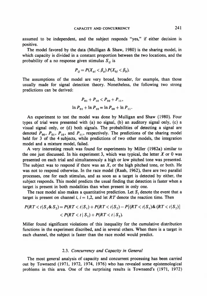
A very interesting result was found for experiments by Miller (1982a) similar to the one just discussed. In his experiment 3, which was typical, the letter X or 0 was presented on each trial and simultaneously a high or low pitched tone was presented. The subject was to respond if there was an X, or the high pitched tone, or both. He was not to respond otherwise. In the race model (Raab, 1962), there are two parallel processes, one for each stimulus, and as soon as a target is detected by either, the subject responds. This model predicts the usual finding that detection is faster when a target is present in both modalities than when present in only one.

The race model also makes a quantitative prediction. Let Si denote the event that a target is present on channel i, i = 1,2, and let RT denote the reaction time. Then

P(RT< tIS,&S,)=P(RT< tIS,)+P(RT< tlS,)-P[(RT< tlS,)&(RT< tls,)]

< P(RT < t I S,) + P(RT < t I S,).

Miller found significant violations of this inequality for the cumulative distribution functions in the experiment discribed, and in several others. When there is a target in each channel, the subject is faster than the race model would predict.

2.3. Concurrency and Capacity in General

The most general analysis of capacity and concurrent processing has been carried out by Townsend (197 1, 1972, 1974, 1976) who has revealed some epistemological problems in this area. One of the surprising results is Townsend’s (1971, 1972)


finding that serial and parallel systems are often indistinguishable on the basis of the reaction time distributions. Even if the probability distribution of the completion time for every process is known, any parallel model can be mimicked by an equivalent serial model, and vice versa, although occasionally a model of one type used to mimic a model of the other type will be bizzare (Townsend & Ashby, 1983).

The outlook for analyzing tasks is more optimistic, however, if processes can be prolonged by manipulating experimental factors. For instance, Townsend and Ashby (1983) have shown that a large class of stochastic parallel models are incapable of predicting that factors prolonging different processes will have additive effects on the mean reaction times. They also discuss other procedures for restricting the set of models compatible with a given set of data. See also the results of Schweickert (1978), discussed below.

In a serial system, every pair of processes is sequential and in a parallel system, every pair of processes is collateral. Suppose each process operates on an element specific to that process. Then a serial system “processes elements one at a time, completing one before beginning the next,” while a parallel system “begins processing elements simultaneously; processing proceeds simultaneously, but individual elements may be completed at different times” (Townsend, 1974, p. 139).

In either parallel of serial systems, if processing stops when a certain element is completed, the processing is said to be self-terminating. If processing stops only after all elements are completed, then processing is said to be exhaustive. For either kind of system, the time interval between the completion of two elements is called a stage. Stage i, then, is the interval between the completion of element i-l and completion of element i, numbered in order of completion.

Suppose there are n input elements to be processed. According to Townsend’s (1974) definition, if the number of inputs has no effect on processing time or accuracy, then the system has unlimited capacity, while if there are such effects, the system has limited capacity.

In the “standard serial model” items are processed one at a time, and the mean time required to process each item is the same. The time required to process each item does not depend on how many elements are in the system. Therefore, capacity is unlimited both at the level of the individual elements and at the level of the minimum process time, i.e., the time until the first element is completed. Capacity is limited, though, in the sense that the time required either for exhaustive or self terminating processing depends on how many elements there are.

In the “standard parallel model,” elements are processed concurrently, and the mean processing time for each element is the same. Suppose the processing times for the individual elements are independent random variables. Then capacity is unlimited at the individual element level. Capacity is also unlimited for self-terminating processing, since the time for processing a given item does not depend on the number of items. There is supercapacity at the level of the minimum processing time, because this time decreases as the number of elements increases. But capacity is limited for exhaustive processing, since the time when the last element is completed increases as the number of elements increases.


It is interesting to note that a parallel model with unlimited capacity at the level of exhaustive processing is possible. Suppose that as each element is finished, the released resources are distributed to the remaining elements, so their processing speeds up. Suppose also that in each state, the processing times of the individual elements are exponentially distributed.

Let v be the processing rate of one element when it is the only input. When n elements are input, suppose each has the rate u. Since each elements’s processing time is exponentially distributed, the time until the first element is completed is exponentially distributed with rate

i v = nv. i=l

After the first item is completed, the total capacity is divided among the remaining n - 1 elements, so each now has a rate nu/(n - 1) (see Fig. 7). The second stage is exponentially distributed with rate

n-1

C nv/(n - 1) = nv, i=l

the same rate as for the first stage. With this pattern, the mean execution time for each stage will be l/nv, so the mean

time to complete all elements is

But, this is the same as the time required to complete one element when it is the only input. Therefore, this model has unlimited capacity with respect to exhaustive processing, that is, the mean time required to complete the processing of n elements is independent of n. Such flat functions relating reaction time to n are sometimes found in experiments, e.g., Egeth, Jonides, and Wall (1972). It turns out that there are serial models which also predict such flat functions, but the assumptions necessary for them are so counterintuitive as to make them extremely implausible (Townsend, 1972, 1974).

I Y I nv/(n-II 2 ” 2 nu/(n-ll I w/2 3

“. 3 nv/(n-l) . . . . I “”

. . . . l 2 w/2

” y n-l nv/\n-l)

stage I stage 2 Stoge n-l Stage n

FIG. 7. A parallel model with the unusual property that the mean time to complete n elements is the same as the mean time to complete 1 element.


2.3.1. Equivalent Serial and Parallel Models

One of the most important theoretical results on serial and parallel models is that they often make identical predictions about reaction time distributions. This linding implies, of course, that there are limits to what we can determine about processing systems by studying reaction time.

As an example of this mimicking, consider a standard serial model with the processing time of each stage having an exponential distribution with rate u. Then l/u is the mean processing time for each stage. When IZ elements are processed, one will be processed first, one second, and so on. Suppose all processing orders are equally likely.

Now consider a parallel model. Suppose when n elements are presented, the duration of stage i is exponentially distributed with rate

v(i, n) = 24

n-i+l’

At stage i there will be n - i + 1 elements being processed simultaneously each with rate v(i, n), so the rate of stage i is

n-i+1

c u i=l n-i+1 =

u,

and the mean processing time for each stage is l/u, the same as for the standard serial model.

One can also find serial models that mimic the standard parallel model. We have made several particular assumptions in this example, that the stages have exponential distributions, that processing time does not depend on the particular element being processed, and so on. But these assumptions are not necessary, and a set of relatively simple and very general conditions under which serial and parallel models will mimic each other is provided in Townsend (1976). The conditions are in the form of functional equations relating the density functions of the stage durations. Conditions and properties that may aid in experimentally discriminating parallel and serial systems are discussed in Townsend and Ashby (1983).

2.3.2. Power and Energy

Recently Townsend and Ashby (1978, 1983) have developed a mathematical framework for capacity in terms of power and energy. In this conception, power is the rate of energy disbursement per unit time, while energy is the integral of power and can be represented as the amount of work done over an interval of time.

Capacity as power or energy may be related to a stochastic approach through the hazard function of a nonhomogenous Poisson process (Townsend dz Ashby, 1983, Chap. IV). The hazard function H(t) represents the instantaneous rate of completion of an item (or unit of work) or, equivalently, represents the conditional probability of completion of an item, given that it has not been completed until that time. Therefore,


the cumulative probability distribution function that a new unit of work (e.g., reading a letter) is finished over a duration of time can be written

F@) = 1 _ e -@W) df’.

Treating work or energy as a positive integer-valued variable then permits the average amount of expended energy over an interval t to be expressed as

AE(t) =j’H(t’),dt’; 0

This quantity gives the average number of work units completed. Also, it follows that

dAE(t) ~ = H(t) = Average Power = AP,

dt

that is, H(C) equals the average power disbursed at instant t. This formulation has the advantage of tying together a probability distribution on work and energy, as well as the average energy or power expended, to reaction time distributions.

Finally, at any point in time t, if there are n processes working in parallel, each with hazard function H,(t) (i = 1, 2,..., n), then the overall capacity in terms of average power may be expressed as

and consequently Total AP = t H,(t),

i=l

That is, the total average energy equals the sum of the separate average energies. This completes our discussion of concurrent processing within the central

mechanism, and we now turn to the idea that processes not requiring the central mechanism can execute concurrently with those that do. It is worth noting that the models above can be considered as models of concurrent processing in any single resourse, and are not restricted to the central mechanism necessarily.

3. CONCURRENT PROCESSES OUTSIDE THE CENTRAL MECHANISM

In this section we will discuss the way the processes in a task are arranged, and the role of the processes using the central mechanism, as far as we understand it. We will begin with Sternberg’s (1969) additive factor method which has produced a major advance in the investigation of the way mental processes are organized.


3.1. The Organization of Processes

Sternberg considered, as Donders (1969) did, the case of mental processes in series. Suppose to perform a task a set of mental processes such as perceiving and deciding are executed one after the other. The response time is the sum of the times required to complete each processes. Stemberg noted that if two experimental factors are manipulated, and each affects a different process in the series, then the combined effect of both factors will be the sum of their individual effects.

Two converse ideas are used to analyze a task into its constitutent processes with the additive factor method. First, if two factors have additive effects, it is likely that each affects a different process. Second, if two factors have interactive effects, it is likely that they affect the same process.

Neither the converse statements is a necessary conclusion from the assumptions, of course. But the first statement seems to provide the most parsimonious explanation for additivity between two factors, and its many empirical applications have been fruitful. There have also been several new theoretical developments in interpreting additivity (McClelland, 1979; Schweickert, 1978; Townsend & Ashby, 1983). These will be discussed below.

In retrospect, it can be seen that the second statement provides only one of several plausible explanations for an interaction between two factors. One explanation of how two factors could affect different processes, and yet interact, was offered by Sternberg (1969, p. 287) in his paper on the additive factor method. Suppose the rate of a process is affected by the capacity allocated to it. Consider two serial processes, X and Y, which share a source of capacity, so the more capacity allocated to X, the less available to Y. Then if one factor affects X and another affects Y, the factors may interact.

We will now discuss two other ways mental processes might be organized, one with an essentially serial orientation developed by McClelland (1979) and one with a concurrent orientation suggested by Schweickert (1978). Each leads to a special interpretation of interactive effects of factors.

3.1.1. The Cascade Model

Donders (1969) assumed that a process must finish before its successor can start. Another possibility is that when a process begins execution it immediately starts sending output to the succeeding process, just as a person washing dishes can pass clean dishes, one by one, to the person drying them. The most developed psychological theory of such a system is the cascade model of McClelland (1979). It is a type of linear systems model.

A process Y in a cascade is said to be an immediate successor of a process X if the output of X is used as the input to Y. In a cascade, one process may preceed another in this sense, and yet both may be executing at the same time. One consequence is that two successive processes can compete to us the same resource at the same time.

The output of a process, called its actiuation, is a continous quantity whose level at


any given time depends on two parameters of the process, its rate and asymptote. The process with the slowest rate is called the rate limiting process.

One of the exciting properties of a series of processes in cascade is that if each of two experimental factors affects the rate of a different process, the factors will behave as additive factors, provided the process with the slowest rate remains the slowest (McClelland, 1979). Townsend and Ashby (1983), taking a different approach, show conditions under which a general linear system could reveal exact factor additivity. This result suggests that the vast literature describing factors found to have additive effects would still be valuable, even if the human information processing system were found to be a cascade system.

Since experimental factors can affect either the rate or the asymptote of a process, several outcomes of factor manipulations are possible. For instance, if each of two factors affects a different process, but, one affects the asymptote of some process, while the other affects the rate of the rate limiting process, an interaction can occur. A classification of the various outcomes and their interpretations is given in McClelland’s (1979) article.

3.1.1.1. DOES SUCH PROCESSING OCCUR? This will not be an easy question to answer. We first consider a general, but qualitative, empirical problem, and then a quantitative problem, specific to one way of formulating the model.

3.1.1.1.1. Qualitative Issues. Several relevant experiments were done by Miller (1982b). He defines a continuous model to be one like the cascade model in which as soon as a process begins execution it immediately begins sending information to succeeding processes. He calls a model such as Donders’ (1969), in which a process must be completely finished before its successor can begin, a discrete model. Miller’s experiments address the issue of whether information useful for response preparation can be extracted in an early process and decrease reaction times. In some of Miller’s experiments this occurred, but in some it did not.

His experiments use the fact that it is faster to prepare two responses made by the same hand than two made by different hands (Rosenbaum, 1980). In one of Miller’s experiments, a capital letter was presented on each trial, and the subject identified it by pressing a button. Two of the stimuli were physically small and two were large; a typical set consisted of a large capital S, a small capital S, a large capital T an a small capital T. If the two large letters were assigned to fingers of one hand while the two small letters were assigned to fingers of the other hand, the subject was faster than if there were no relationship between stimulus characteristics and the hand used in responding. An analogous, although smaller, increase in speed was found when the large and small versions of the same letter were assigned to the same hand. Miller explained this by saying that information about the size of the stimulus may be available before the stimulus is completely identified, and the size information, if relevant, can be used to speed response preparation. Information about which letter was presented can also speed response preparation.

It is natural for a continuous model to predict that response preparation can be


sped up by information from earlier processes. A discrete model can also account for the data if stimulus identification were carried out in two separate processes, a decision about size and a decision about the letter. (See the discussion of separable and integral dimensions below for more on this idea.) If size is related to which hand is needed, then when the decision about size is completed, the information is available to a response preparation process, even though more processing must be completed for stimulus identification. The subject may be able to choose which of the two decisions, size or letter, is made first, depending on which is relevant to response preparation. Some evidence that the order of decisions can change depending on the experimental conditions is given by Schweickert (1983).

In this experiment of Miller’s early information could be used to speed response preparation. But in other experiments, it could not. We will discuss one of these. A pilot experiment showed that subjects are faster to identify which one of a pair of letters was presented when the letters are visually dissimilar, e.g., (M, U} then when they are simillar, e.g., {M, NJ. Thus one would expect that visual similarity could serve as a cue for response preparation.

The experiment proper was an identification task with stimuli {M, N, U, V). In one condition the visually similar pair (M, N) was assigned to one hand while the pair {U, V), also visually similar, was assigned to the other hand. In another condition, there was no relationship between visual similarity and hand. There was no decrease in reaction time when the visually similar letters were assigned to the same hand. If continuous processing is occurring in this task, the subject is unable to make use of information from early processes to shorten later processes. But this behavior seems inefficient for a system with continuous processing.

To summarize, Miller’s experiments show that either continuous processing does not occur between early and late processes in some tasks, or else its effects are very subtle.

3.1.1.1.2. Quantitative Issues. Many of the results in McClelland’s (979) paper were established by computer simulations. Ashby (1982a) made it possible to derive exact predictions from the model by working out the reaction time distribution function for McClelland’s model.

He found that the model does indeed predict additivity for mean reaction times, to a close approximation, when new processes are inserted and when factors selectively influence different processes. On the other hand, there are two experimental findings contrary to the predictions of the model. The first is that as mean reaction time increases the variance increases substantially. The second is that in some tasks the durations of certain stages have exponential distributions. Evidence for this important finding is given by Ashby and Townsend (1980), Ashby (1982b), and Kohfeld (1981). Both findings are contrary to the model as it now formulated. It remains to be seen whether a reformulation of the model can accomodate these findings.

3.1.2. Concurrent Processing Models

Many people have stated that some, if not all, mental processing is concurrent. To


give a very few examples, parallel processing has been proposed for multidimensional discrimination by Egeth (1966), for iconic storage by Haber and Hershenson (1973), and for neurological mechanisms by Anderson et al. (1977) and Grossberg (1973). Double stimulation, double response experiments show that processing is not wholly serial, otherwise the time required to make the second of two responses would be at least as long as the sum of the times required to respond to each stimulus separately. But such experiments also show that processing does not occur concurrently and without interference, otherwise the responses of a subject responding to two signals would be as fast as if he were responding to each separately. In other words, processing is neither purely concurrent nor purely sequential.

Early models postulating mixtures of concurrent and sequential processing were devised by Christie and Lute (1956) and by Davis (1957). Christie and Lute address the mathematical problems raised by processes with stochastic durations in such systems. These problems are formidable, and although some progress has been made recently (Bloxom, 1979; Fisher & Goldstein, 1983; Schweickert, 1982; Townsend & Ashby, 1983), they are outside the scope of this review. The model by Davis (Fig. 8) specifies the locus of several specific processes in a double stimulation task. He tried, with some success, to find estimates from the literature of the durations of some of the processes. These were used to infer the durations of other processes in the model, and to make predictions. This procedure is limited, of course, to those rare experiments for which good estimates of process durations are available. Nevertheless, Davis’s model is more plausible for double stimulation tasks than a serial model would be.

Sl TIME -

SP STIMULUSY

I-I-I I I I

I I

I I

RESPONSE 2 1

FIG. 8. A model by Davis of a task involving concurrent processing. The stimuli Sl and S2 are presented, separated by the interval I. RT, is reaction time to stimulus S,. RT, is reaction time to stimulus S,. ST, is sensory conduction time for stimulus S,. ST, is sensory conduction time for stimulus S,. CT, is central time for stimulus S,. CT, is central time for stimulus S,. CRT, is central refractory time for stimulus S,. CRT, is central refractory time for stimulus S,: CRT, does not overlap CRT,. PT, is motor conduction time for response 1. PT, is motor conduction time for response 2. X is the amount of delay in the second reaction time. Note. From “The human operator as a single channel information system,” R. Davis, Quarterly Journal of Experimental Psychology, 1957, 9, 119-129.


Some processes in Davis’s model cannot start until certain others have finished. For example, the motor conduction for response 1, PT,, does not start until the central time for stimulus 1, CT,, is completed. Two processes are said to be sequential if the completion of one must precede the start of the other. (Two sequential processes need not be adjoining, for instance, ST,, and CRT, are sequential processes.) There are also cases in Davis’s model in which more than one process can be executed at a time. For example, the motor conduction for response 1, PT, , may go on at the same time as the sensory conduction for stimulus 2, ST,. Two processes like these which are not ordered with respect to each other are said to be collateral. Note that two processes need not be executed simultaneously to be called collateral, it simply must be the case that the completion of one is not a precondition for the start of the other.

In Davis’ model, two processes are sequential if one provides input to the other, or if each requires the central mechanism. Otherwise, they are collateral.

A diagram in the form of Fig. 8 representing the processes in a task is called a Gantt chart; it is useful for displaying the process durations, but awkward for displaying the execution order. To emphasize execution orders, a directed network can be used to represent processes. Fig. 9 gives a network representation for Davis’s model in Fig. 8. In Fig. 9 it is not possible to start at a vertex and follow a path along the arcs and vertices back to the starting vertex, traversing each arc from tail to head. Therefore, the network is said to be acyclic, and the processes are partially ordered.

The problem of coordinating a system with concurrent processing is not simple. If a central executive controls the starting and stopping of every process, than a long queue of requests and messages can accumulate at the central executive, slowing the whole system. On the other hand, if the processes are autonomous, then other problems can arise; one of the most important of these is determinacy, which we discuss next.

3.1.2.1. DETERMINANCY. In systems with concurrent processing, it is important that the outputs of the processes not be affected by the other order in which they are completed. Imagine a calculator with two keyboards designed for concurrent operation, but only one display register. If two people, in a kind of computational duet, are to calculate the quantity (a + b)/c + d), one person could work on (a + b) while the other autonomously worked on (c + d). But the final steps to be taken will

FIG. 9. Davis’s model represented as a directed acyclic network.


depend on which quantity, (a + b) or (c + d), is completed first. The two people will need some prior agreement about who uses the display first, or else they will need to confer with each other from time to time during the calculations. Either way, some of the advantages of concurrent processing are lost. Clearly, to make full use of concurrent processing, without heed for the order in which processes are completed, a certain minimal memory storage capacity must be available. What is required?

Let X denote the event that process x has started, and let 5 denote the event that x has terminated. An execution sequence is a list of starting and terminating events, - - x, y, x,..., arranged in an order which satisfies the precedence constraints of the task network.

Let M = (M, , M, ,..., M,) be the set of memory locations available to the system. Let the set of values V be the set of all possible inputs and outputs of mental processes. Each memory location contains an element of V. As the task is performed, a particular location Mi will take on a succession of values. If e is an execution sequence, let V(M,, e) be the list of successive values occupying M,. At the start of the task, each location contains some value and the list of these values is called the initial state of the task. A system is determinate if for all memory cells Mi, 1 < i < m and all execution orders e and e’, V(M,, e) = V(M, , e’) for all initial states. Loosely speaking, a system is deteminate if every execution order yields the same sequence of results in each memory location. Weaker conditions are sometimes defined.

A process x reads information from a set of memory locations. Call this set the domain of x, D, c M. Likewise, x writes into a set of memory locations, and we will call this set the range of x, R, c M. The range or the domain of x may be empty. Nondeterminancy arises when one of a pair of concurrent processes writes into the range or domain of another. An example would be a dichotic listening experiment where information from one ear supplants information form the other in memory.

Coffman and Denning (1973) provide a sufficient condition for a system to be determinate. Two processes x and y are said to be noninterfering if either

(a) x precedes or follows y in the task network, or

(b) R,nR,=D,nR,=R,nD,=#.

The following theorem gives a condition sufficient to prevent indeterminacy:

THEOREM. Task system consisting of noninterfering processes are determinate.

The theorem is proved in Coffman and Denning (1973), a source for more information on this topic. We now turn to the issue of speed-accuracy trade-offs.

3.1.2.2. TIME-COST TRADE-OFFS WITH CONCURRENT PROCESSING. It is well known that a subject can improve his accuracy in a task if he is willing to take more time to complete his response (e.g., Pachella, 1974). Often there is a cost charged by the experimenter for each error made and for each unit of time elapsing after a deadline to respond. The payoff induces the subject to perform at some subjectively

480/28/3-3


optimal balance of time and cost. The time-cost function for the task gives for each time T the cost or gain for completing the task with response time T.

The speed-accuracy trade-off is usually discussed without considering separate processes. These can be incorporated in the speed-accuracy analysis in the following way. Suppose each process in the task has an associated time-cost function, which gives its contribution due to errors to the total cost of completing the task. Generally, the cost of finishing the process quickly will be very high (because of many errors), and the cost will decrease as more time is allocated to the process. There may be a point beyond which the cost of completing the project begins to rise because of memory loss. In short, cost is a concave upward function of time (Fig. 10). Note that there is never a reason to allocate a time to the right of the minimum cost because allocating a smaller amount of time will yield performance that is faster and cheaper. Supdose the cost of completing the task is the sum of the costs of completing each separate process plus the payoffs related to response time.

It is usually not a simple matter to determine the amount of time to allocate to each process in order to minimize the total cost (for procedures, see Kelley, 1961; and Ford and Fulkerson, 1962). But once the subject has found an optimal schedule, there is a simple relationship which holds for the allocated execution times (Berman, 1964).

Suppose the processes in a task are partially ordered; that is, they are arranged in a directed acyclic network. Let (dC,/dti) 1 t? be the slope of the time-cost function for process xi when the execution time of Xi is t?. For a point n in the task network, let the set of all processes terminating at n be E(n) (“entering n”) and let the set of all process starting at n be F(n) (“following n”). Suppose the values of tT have all been chosen so the total cost of completing the task is minimized. Berman’s (1964) result is that when the schedule is optimal, for every point it in the network, the sum of the slopes of the time-cost functions of all processes entering n is equal to the corresponding sum for all processes leaving n, i.e.,

We will illustrate this principle with a simple example. Consider a task with two processes xi and x2 in series. Given the penalities set by the experimenter for errors,

time t

FIG. 10. The cost due to errors of completing a process in time t is high for small values of f, and may be high for large values of t because of information loss from memory.


exceeding the deadline, and so on, there will be an optimal time T for the subject to complete the task. Suppose in this case T = 6. (See the references above for procedures to find the value of T.) Let the time allocated to x, be f1 > 0 and that allocated to x2 be t, > 0. Then t, + t, = 6.

Suppose as more time is devoted to x,, the errors made by x, decrease, and the cost C, associated with x1 decreases according to the function C, = 4/t,. Suppose the analogous time-cost function for x2 is C, = l/t2. (These functions were chosen for illustrative purposes only, not as representative of the actual forms of such functions.)

Consider the situation in which an equal amount of time is allocated to each process, so t, = t, = 3. The cost is 4 + 4 = 5, which is not optimal. The rate of decrease in cost for increasing t, by a small amount beyond 3 is

de, 4

dt, =-??’ t,=3

On the other hand, the rate of increase in cost for decreasing tz below 3 by a small amount is

G 1 -- dt, = 7’ t*=3

Hence there would be a decrease in the sum of the costs C, + C, if t, were increased by a small amount while t, were decreased by the same amount, keeping the total time at t, + t, = 6.

Changes in the times 1, and t, allocated to x1 and x2, respectively, will not be profitable if they are chosen so that

dC, dC, -=- dt, dt,

This equation is equivalent to the equation 4tf = t:. Since t, + t, = 6, the optimal values are t, = 4 and t, = 2, and these yield a total cost of C, + C, = 1.5.

This principle, that the sum of the slopes of the time-cost functions for processes entering each node is equal to the corresponding sum for processes leaving the node is analogous to one of Kirkoffs laws for electrical networks, namely that the sum of the currents entering a node equals the sum of the currents leaving it. For task networks, when process execution times are optimal, the sum of the marginal costs going into each node equals the sum of the marginal costs going out. This principle may be useful in connecting the analysis of the speed-accuracy trade-off for a task to the analysis of the task in terms of its constitutent processes.

3.1.3. Empirical Analysis of Partially Ordered Sets of Processes

If, as Donders (1969) assumed, every pair of processes is sequential, the system is serial, while if every pair of processes is collateral, the system is parallel. One of the


surprising results of research in this area is Townsend’s (197 1, 1972) finding that serial and parallel systems are often indistinguishable on the basis of their reaction time distributions. The outlook for analyzing tasks is more optimistic, however, if processes can be prolonged by manipulating experimental factors. For instance, Townsend and Ashby (1983) have shown that a large class of stochastic parallel models are incapable of predicting that factors prolonging different processes will have additive effects on the mean reaction times.

Tasks involving a partially ordered set of processes, such as those in Davis’s (1957) model (Fig. 8,9), can be investigated using the method of latent network theory, developed by Schweickert (1978, 1980, 1983). This method uses the fact that when the durations of processes in a network are prolonged, their behavior reveals a great deal about the network. To keep the mathematics tractable, the method, in its present state of development, assumes that process durations are deterministic, rather than stochastic. With this assumption, it turns out that the equations describing the effects of prolonging processes are quite simple, even for processes arranged in a complex unknown network.

The amount of time by which a process y can be prolonged without increasing the reaction time is a nonnegative real number called the total stack for y, sCy, r). In Fig. 8, for example, the total slack for process ST, with respect to the response of the second stimulus is X. Suppose process y is prolonged by Ay. If Ay is less than s( y, r) no increase in response time is observed. If A y is greater than s(y, r), then an amount s(y, r) of the prolongation is used to overcome the slack and the remainder increases the reaction time. Let At(A y) denote the increase in reaction time when y is prolonged by A y. Then

Ar(Ay) = 0 if AY < S(Y, r),

= AY - S(Y, r) if Ay < s( y, r). (2)

The following equations, derived in Schweickert (1978), describe the effects of prolonging two processes. Let At(Ay, dz) be the increase in reaction time when processes y and z are prolonged by Ay and AZ, respectively; other terms are defined analogously. If y and z are collateral processes (y and z in parallel is a special case), then

At(Ay, AZ) = max (At(Ay, 0), At(0, AZ)}. (3)

Suppose y and z are sequential processes, with y preceding z. The amount of time by which y can be prolonged without delaying the start of z is called the slack from y to z, s( y, z). If y and z are prolonged by Ay and AZ, and if Ay and AZ are not too small, then

At(Ay, AZ) = At(Ay, 0) + At(0, AZ) + k( y, z), (4)

where k(y, z) = s(y, r) - s( y, z) is called the coupled slack from y to Z.


Equation 4 shows that if k(y, z) = 0, prolonging y and z will lead to additive effects. Usually, however, the effects of prolonging two processes will interact. The interactions have a different form for collateral and sequential processes, so these two possibilities can usually be distinguished, although, as is typical for these questions, there are some conditions under which the issue cannot be resolved.

Further information can be obtained by prolonging processes. The following is a brief summary and the details are in Schweickert (1978). If one process precedes another, the method can usually determine which comes first, although some cases are left unresolved. For example, the method does not reveal the execution order of processes in a purely serial system. One important novel finding is that the method can be used to calculate an interval for every process within which its duration lies. Further, an experiment to investigate a task can usually be designed in such a way that more equations than unknown parameters are generated, so theories based on this method can readily be falsified. This feature makes the simplifying deterministic assumption less perilous.

3.2. The Nature of Cental Processes

While many psychologists agree that there is a central mechanism of some sort which imposes limits on human information processing, there is no clear agreement on what the functions of this mechanism are. We will consider the major possiblilities which have been proposed.

3.2.1. Decisions

The information associated with a stimulus is -log p, where p is the probability that the stimulus is presented. Following Donders (1969) and Hick and Welford (1956), we define a decision about a stimulus to be a process prolonged by increasing the information value of the stimulus. According to Welford (1952, 1959, 1967), decisions about two stimuli can not be made simultaneously because each decision requires the exclusive use of the central mechanism.

A stimulus has values on a number of dimensions, such as color, shape, and so on, and we will say that a decision about a dimension is a process prolonged by increasing the information associated with the dimension. Suppose two equiprobable stimuli are possible in an experiment, a red square and a blue triangle, and the subject is to make a different response to each. If the subject must decide about one dimension, say color, first, and then about the other, shape, he must make two one-bit decisions. But since there are only two stimuli in the experiment, theoretically the subject could make one one-bit decision, between the two alternatives red square and blue triangle. Is it ever possible for the subject to operate in this latter, more efficient mode?

3.2.1.1. INTEGRAL AND SEPARABLE DIMENSIONS. An answer is suggested in the distinction (Garner, 1970, 1974; Lockhead, 1966) between integral and separable dimensions. “If in order for one dimension to exist, the other must be specified, then

256 SCHWEICKERTANDBOGGS

the dimensions are integral” (Garner, 1974, p. 136). If dimensions are not integral, then they are separable. For example, a hue cannot be presented without also presenting some level of brightness, so hue and brightness are integral dimensions. But a hue can be presented without a level of pitch, so hue and pitch are separable dimensions. Garner’s statements suggest the hypothesis that if two dimensions are integral, the subject can make a single decision about them (Garner, 1974, p. 149). For separable dimensions, the subject first processes one dimension, then the other. Furthermore, in the special case in which the subject has enough information to respond correctly if the determines the value the stimulus takes on for only one of its dimensions, then, according to Garner, “selective serial processing is an optional process relevant only to separable dimensions, in which usually the better (easier to discriminate) dimension is processed first, and presumably no further processing takes place if a decision [about which response to make] can be made on the basis of the first dimension” (Garner, 1974, p. 139). According to Garner, two dimensions can be decided about simultaneously, if they are integral, although in that case there is only one decision, so Welford’s hypothesis that only one decision is made at a time would not be contradicted by such an occurrance.

3.2.1.2. IDEOMOTOR COMPATIBILITY. Is it possible for two completely different decisions to be made concurrently? This may occur if at least one of the decisions is made automatically, see below. The only data known to the authors which strongly suggest the possibility of two concurrent decisions is from an experiment by Greenwald (1972). Suppose subjects are to respond to the spoken word “left” by saying the word “left.” The feedback from the response, which the subject will hear, resembles the stimulus, and in such cases the stimulus and response are said to be ideomotor compatible. According to Greenwald, if two stimuli have ideomotor compatible responses, the decisions about the stimuli can be made concurrently, perhaps because they bypass the central mechanism completely.

In a double stimulation experiment to test these ideas, Greenwald (1972) presented subjects with an arrow pointing either left or right and with a spoken word, either “left” or “right.” In the condition of interest, the subject moved a toggle switch in the direction indicated by the arrow and repeated the word, so the stimulus-response mappings were ideomotor compatible. The decision about the arrow was prolonged by increasing the number of arrows possible in a block, that is, in some blocks the arrow always pointed in the same direction, and in other blocks it pointed either left or right. The decision about the word was prolonged analogously. Let dt(dw, 0) be the increase in reaction time produced by increasing the number of alternative words, let dt(0, da) be the increase produced by increasing the number of alternative arrows, and let dt(dw,da) be the increase in reaction time produced by both manipulations. Then in Greenwald’s (1972) data, Eq. 3 holds,

dt(dw, da) = max{dt(dw, 0), dt(0, da)}.

This equation is consistent with Greenwald’s idea that the decision about the word

328 ROBERT LJENSEN

Hence, the LS-eigenvector of [ W*] approach yielding w: scores has more flexibility in deriving consistency adjustments to rij values than does the PR-eigenvector of [R] approach yielding ui scores. Thef(b, c) component is given in terms of the b and c parameters as

m cl = &. (13)

Given [RI, the PR-eigenvector can be determined by only knowing the a parameter, whereas the LS-eigenvector allows more adjustment freedom with two parameters. These b and c parameters are derived from the ESS minimization algorithm.

In the limiting case where [R] is of rank one (implying perfect response consistency), the parameters are a = b = c = 1. When [R] is of higher rank, because of response inconsistency, these parameters diverge.

The patterns of divergence of 1, CR, ui, ~7, ESS, a, b, and c values when [R] varies in rank are illustrated in Table 4. In Alternative 1, the [R] matrix is rank one. In Alternatives 2 through 7, the size of rJ2 steadily increases ceteris paribus, thereby creating higher rank response inconsistency. The wr weights are much more in line with respondent judgments than are the ui weights which are not intended to

*. * mnnmtze aggregate ul, squared error from rij responses. Accordingly, the ESS explodes under the PR-eigenvector of [R] scaling method as the rank of [R] increases.

In Alternatives 8 through 13 of Table 4, the importance of r3? decreases ceteris paribus. Once again, the w: weights diverge from ui weights as rJ2 changes. This is evident once again in the explosion of ESS the PR-eigenvector of [R] approach.

6. NONUNIQUENESS OF LSM

In practice, LSM and EM generally provide unique scaling solutions to scaling of [R] matrices and the corresponding implicit consistency adjustments. It is, however, possible to specify [R] matrices that have certain symmetries and high levels of response inconsistency that result in multiple LSM solutions yielding minimum least square error. I discuss and illustrate these circumstances in Jensen (1984). Nonuni- queness is easily detected and is not likely to arise in practice, especially when the CR & 0.10 rule of thumb is applied to consistency adjustments. At absurdly high CR = 6.13 and A = 10.1 levels, the following matrix illustrates a hypothetical case in which three alternative LSM solutions arise:

Alternative LSM Solutions


3.3. The Nature of Noncentral Processes

In her excellent review of the resource demands of mental processes, Kerr (1973) pointed out that there are essentially two ways to explain why the time required to process two signals together is less than the sum of the times required to process each signal alone. The first explanation, discussed in a previous section, is that some central processing is concurrent. The second explanation, which we are discussing in this section, is that some processes do not require the central mechanism, and hence can be executed concurrently with those that do.

Which processes require the central mechanism and which do not? This is an important question to which the best-and perhaps only-answer is empirical. In her review, Kerr (1973) made a thoughtful attempt fo find an answer. After discussing limited capacity theories and methodological issues, she presented a survey of relevant experiments, primarily those using dual tasks.

Kerr’s (1973) reasoning was as follows: Suppose two tasks, A and B, are performed alone and, on another occasion, together. Suppose performance on A is no better when combined with B than when performed alone, while performance on B is worse when combined with A then when performed alone. Then it is reasonable to suppose that the two tasks require the same resource. Of course the resource need not be the central mechanism, and resources need not be relevant at all, since dual task interference may occur because additional processes might be inserted into the tasks when they are performed dually (Duncan, 1980). Nonetheless, dual task interference gives strong clues about the use of the central mechanism.

Kerr (1973) tried to determine whether each of several types of mental processes require the central mechanism. She concluded that two types of processing, (a) encoding and (b) executing a movement, until physically stopped, do not require the central mechanism and will not interfere with concurrent processing on it.

The evidence on encoding is from an experiment by Posner and Boies (1971) in which a warning signal was presented, followed by a letter, followed one second later by another letter. With one hand the subject indicated whether the letters were the same or different, ignoring case. With the other hand, the subject responded to a white noise probe, presented on half the trials. ,

Presumably, the subject is encoding the first letter in the tirst 300 ms after it is presented. Nonetheless, reaction times to the noise probe when it was presented 50, 150 or 300 ms after the onset of the first letter were less than or equal to reaction times to the probe when it was presented in the intertrial interval. Likewise, the letter match reaction times were no longer when the probes were presented 50, 150, or 300 ms after the first letter than when no probe was presented. The absence of increases in reaction time suggests that encoding occurs concurrently with the auditory processing and without interference.

However, in the Posner and Boies (1971) experiment the probes used as a basis for comparison were presented during the intertrial interval. As Ogden, Martin, and Paap (1980) point out, this is not the same as a base line condition in which the probe is presented alone. In an experiment similar to that of Posner and Boies (197 1 ), they


found that reaction times to probes presented 50 ms after the first letter were longer than reaction times to probes presented alone. They also found that if the probability of a probe occuring during the intertrial interval was as great as the probability of its occurring later, then reaction times were longer to probes presented 50 ms after the first letter than to probes presented in the intertrial interval.

The experiment of Ogden, Martin, and Paap (1980) shows that encoding cannot be ruled out as a process which interferes with probe processing. The question of whether encoding necessarily interferes with probe processing is left open because some process other than encoding may be the source of the delay in their experiment.

The evidence that lead Kerr (1973) to say that responding does not use the central mechanism is from an experiment by Ells (1973, Experiment 1). Subjects made an angular movement with one hand and were stopped mechanically. With the other hand, subjects responded to a tone in a two-choice identification task. Reaction times to tones presented after the movement had begun were no longer than in a control condition in which subjects merely watched the angular movement take place. The absence of an increase in reaction time when the movement occurred is consistent with the idea that the movement does not require the central mechanism.

In this experiment, as Kerr (1973) point out, it is possible that concurrent processing occurred in the central mechanism, but because there was slack capacity, no interference resulted. It is also possible that no interference was observed because the primary and secondary tasks never needed the central mechanism at the same time. Nonetheless, the hypothesis that movement to a physical stop does not require the central mechanism is not implausible and is consistent with the data.

Kerr (1973) concluded that several processes do require the central mechanism. These are (a) multiple input of a group of stimuli, such as a list of words or a sentence, (b) rehearsal, (c)transformations such as adding one to a digit, and (d) responding operations, other than movement to a physical stop. Her survey suggests that processes not needing the central mechanism are likely to be concerned with early input and final output.

3.3.1. Automatic Processes

We call the processes not requiring the central mechanism noncentral processes. Some authors distinguish a subset of these, automatic processes, which have certain additional properties. The term automatic is very old, and the additional properties specified vary from author to author, so there is no universally accepted definition. The differences between hypotheses here are subtle, so rather than organizing our discussion on the basis of the slight theoretical differences, we will loosely organize it by author.

3.3.1.1. SHIFFRIN AND ASSOCIATES. For Shiffrin and Geisler (1973), capacity limitations are due to the characteristics of the short term store. Initial sensory processes can occur in parallel, and have no constraints due to limited capacity. The results these early processes are entered into short term store, where they can serve as a base for further processing.


Initial sensory processes occur automatically. “The extent of automatic processing will be determined in part by past experience. With considerable time and practice we will become familiar with a given stimulus... Eventually the recognition process will make automatic contact with the LTS (long-term store) image without conscious control on the part of the subject” (Shiffrin SC Geisler, 1973, p. 78. See also Schneider & Shiffrin, 1977, p, 4). Shiffrin, Dumais and Schneider (1981) further propose that “Any process that demands resources in response to external stimulus inputs, regardless of subjects’ attempts to ignore the distraction is automatic.” Note that in this view, automatic processes may use resources and may benfit if some central capaicity is allocated to them, but the central capacity is not necessary.

On the other hand, controlled processes are performed through attention by the subject. A part of the short-term store, called short-term working memory, is the resource in which control processes are executed. Controlled processes are based on strategies, and are not automatic. There are several kinds of controlled processes: (a) those, like memory scanning, that locate information in the short-term store; (b) those, like rehearsal, that maintain information in the short-term store; (c) those that transfer information from the long-term store; (d) those that retrieve information from the long-term store; and (e) decisions about strategy.

3.3.1.1.1. Experiments. A large body of experimental work supports the idea that massive practice with a consistent mapping in visual search tasks yields reaction times which increase negligibly with the number of items in the array (Schneider & Shiffrin, 1977; Shiffrin & Schneider, 1977). Such processing is unlikely to be sequential or to demand much capacity.

Furthermore, an experiment by Schneider and Fisk (1982) supports the notion that automatic processes and controlled processes can be executed together without inter- ferrence. In their view, with much practice in visually searching for targets, subjects process targets automatically if items are consistently used as targets or nontargets. If, however, an item is sometimes a target and sometimes a nontarget, processing does not become automatic (Schneider & Shiffrin, 1977; Shiffrin & Schneider, 1977). Using a letter search task, they found subjects could search one diagonal of a 2 x 2 display for an automatic target and the other diagonal for a controlled target with no noticable deficit in sensitivity compared with single task conditions. The dependent measure was accuracy. As they say, it is not possible from their data to decide that automatic processing uses no central capacity, but what is used is at most very little.

3.3.1.1.2. Critique. The conceptions of Shiffrin and Schneider have been criticized by Ryan (1983). He mentions experiments in which reaction times do not increase with the number of items in the display or in the memory set, even though the amount practice is small. In other words,. extensive practice is not needed to produce automatic processing. But then, he claims, the distinction between automatic and controlled processing has no predictive value, and is merely a relabeling of processing as dependent on load or not dependent.

Ryan also presents data suggesting that two controlled processes can be executed concurrently. In the experiments mentioned, the subject was given a fixed memory set


before a block of trials and also a varied memory set before each trial. The data are consistent with the conclusion that the two sets are being searched concurrently, even though reaction time increases with set size for both sets. This conclusion, unfortunately, cannot be evaluated from the data as presented in Ryan’s (1983) theoretical note. But further evidence for such concurrent controlled processing would be extremely interesting.

3.3.1.2. POSNER, SNYDER AND ASSOCIATES. A slightly different definition of automatic processing is given by Posner and Snyder (1975). They postulate that a mental process that does not use the central mechanism has three properties, “the process occurs without intention, without giving rise to conscious awareness, and without producing interference with other ongoing mental activities” (Posner and Snyder, 1975, p. 56). They call such a process automatic. Note that their notion of automaticity includes the proposition, not mentioned by Shiffrin and Geisler, that automatic processes do not interfere with other activities.

Since automatic processes do not interfere with each other, or with processes using the central mechanism, the only resource imposing sequential constraints on processes in this view is the central mechanism. It is possible, however, according to Posner and Snyder (1975), that the outputs of two processes which did not interfere during execution will nevertheless cause either facilitation or interference in later processing.

Posner and Snyder (1975) agree with Keele (1973) that an input automatically activates its memory representations. When a proposition is presented, the individual words access related items in parallel (Anderson & Bower, 1973). Posner and Snyder also suppose that when a particular memory location is activated, the activation automatically spreads to nearbry locations. The limited capacity central mechanism, however, can read from only one memory location at a time.

3.3.1.2.1. Experiments. An experimental procedure for discriminating these two modes of operation was proposed by Neely (1977) for a lexical decision task. In his experiment, subjects were presented with a category prime, such as BIRD, followed by a target letter string. The subject was to indicate whether or not the string was a word. Two factors were manipulated on trials in which the target string was a word. One was whether or not the target was in the category named by the prime; if not, the activation spreading automatically from the memory representation of the prime would not reach the memory representation of the target. The second factor was the conditional probability that the target was in a certain category, given the prime. For example, if the prime was BUILDING, the probability might be high that the target would be a body part, but low that it would be a bird. Conditional probability was assumed to affect a controlled process, under the influence of the subject’s strategy. Neely found that subjects were faster to indicate that a target was a word when it was in the same category as the prime, even when the conditional probability was low that the prime would be followed by a word in the same category. These data support

262 SCHWEICKERTANDBOGGS

the hypothesis that both types of processing took place, and that the automatic processing was not influenced by the subjects strategy.

3.3.1.3. LA BERGE. La Berge’s (1974) model is similar to the Treisman model, in that it is a hierarchical network. Intelligence is distributed in the network under the supervision of the central mechanism. This is a late selection model, in constrast to early selection models like Broadbent (197 1). The distinguishing feature of La Berge’s model is the concept of local learning. Individual nodes in the network can achieve some degree of intelligence, and transform and encode information independently of the central mechanism. This results in a highly parallel system. Local learning naturally occurs as a result of perceptual learning (Gibson, 1969), and many of La Berge’s applications are to skill development in reading.

3.3.1.3.1. Experiments. In support of his model, La Berge (1974, 1975) has done a number of experiments. One notable prediction of his model regards RT practice data collected for visual matching tasks using familiar and unfamiliar characters. The data show, in support of the model, that although initial RTs for matching unfamiliar characters were longer than RT! for familiar characters, RTs for the two types of characters converged over time. This is theoretically due to local learning, and thus greater independence of distributed intelligence, or automaticity.

3.3.1.4. A PRODUCTION SYSTEM WITH AUTOMATIC PROCESSES. A system incor- porating the idea of automatic concurrent processes was proposed by Newell (1980). His goal was to express the Harpy speech recognition system (Lowerre, 1976; CMU Speech Group, 1977) in a form compatible with what is known about human information processing. The model is implemented as a production system. Newell’s paper gives a specification for an entire system, complete with different types of memories and sufficient for recognizing speech. We will discuss the parts of the model having to do with concurrent processing.

A production is a statement with two parts, a set of conditions and a set of actions. When the conditions of the production are all satisfied (or instantiated), the actions are executed. If the conditions of several productions are satisfied at the same time, these productions form a conflict set and, depending on the rules of the particular production system, one or more of the productions in the conflict set are executed.

The condition of a production may contain a variable name; for example, a production system for the Sternberg (1969) memory scanning task might have a production of the form “IF (PROBE = X), THEN SAY YES.” Here X is a variable whose value is assigned by the stimulus. Newell assumes “there is a single mechanism available for instantiating, binding, and using variables so that only one instantiation involving variables can be executed at a time.” He also assumes “productions that do not require the use-variable (UV) mechanism are free to execute asynchronously and concurrently, subject perhaps to lockout restrictions if common structures are accessed.”

Newell points out that productions containing variables correspond to controlled


processes, while those not containing variables correspond to automatic processes. If we suppose that the use of a variable requires a decision, these assumptions are a restatement, in terms of productions, of the ideas discussed earlier that only one decision can be made at a time, but processes not requiring the decision mechanism can execute concurrently. Furthermore, the delay produced by response conflict in tasks like the Stroop task may have something to do with the problem of selecting one production out of the conflict set when several productions all have their conditions satisfied.

3.3.2. Multiple Resources

Processes not requiring the central mechanism may require other resources, nonetheless. Each of these may have its own capacity, which is not necessarily exchangable with that of another resource (Sanders, 1979). One of the first to demonstrate the existence of multiple cognitive resources was Brooks (1967, 1968) and the difficulties involved in analyzing tasks requiring multiple resources were recently been brought to the attention of researchers by Navon and Gopher (1979; Gopher, Brickner, & Navon, 1982).

Suppose a resource such as the central mechanism has a fixed capacity L measured in, for example, items or bits per second. If the performance of a process x would be improved if more of the resource were allocated to it, then x is said to be resource- limited (Norman and Bobrow, 1975). If, instead, no increase in the allocation of the resource to x would improve its performance, x is not resource limited. (In this case, Norman and Bobrow would say that process x is data-limited.)

If no process would benefit from an increase in the allocation of the resource, then the amount of capacity left over is called the slack for the resource. As Norman and Bobrow have noted, although in different terms, if the amount of capacity required to execute a process y is less than the resource slack when process x is executed alone, then x and’y can be executed simulaneously, and the performance of x will be no worse than when it is executed alone.

With one resource the problem is relatively straightforward; either there is enough of it or there is not. With multiple resources, the problem is complicated because a process ordinarily using one resource might switch to another if the first is unavailable, with unpredictable effects on performance. The difficulties in this area are not so much in formulating reasonable theories-many exist in the economics and scheduling literature-but in deciding how to measure the relevant quantities. The problem is severe when resources can be substituted for one another in unknown ways.

How would an experiment establish the existence of resources? It seems likely that two processes x and y both require the exclusive use of some resource if x and y are commutative processes (Bernstein, 1966), that is, if x and y are never executed at the same time, but sometimes x precedes y and sometimes y precedes x. It also seems plausable that two concurrent processes share some resource if performance on one can only improve at the expense of performance on the other. The problem is that


although the existence of a resource may explain a certain behavior, it is not usually intuitively obvious that no other explanation is possible.

3.3.2.1. EMPIRICAL RESULTS. A useful step toward organizing the empirical resource allocation literature was made by Wickens (1980), who reviewed 65 dual- task experiments. In some of these, the modality of encoding (auditory vs. visual), of memory (spatial vs. verbal), or of the response (speech vs. manual) was manipulated. In others, the difficulty of one of the dual tasks was manipulated. The tasks were classified according to their type (detection, tracking, etc.). Reaction-time tasks were further classified according to which process (encoding, memory search, response selection, or response execution) was affected by the difficulty manipulation. Tracking tasks were classified according to whether the difficulty manipulation affected the number of axes to be tracked, the bandwidth, or the dynamics. All this information was combined in diagrams indicating whether the manipulation of one task had an effect on the other.

The results were summarized by Wickens, and as he points out, the pattern is very complex, so we will not attempt to summarize his summary. A simpler pattern might emerge if a classification scheme were based on task variables, such as stimulus-response compatibility and signal discriminability, as Sanders (1979) suggests, rather than on the hypothesized internal processes affected by these variables. To use the latter effectively, one must come to grips with the secondary issue of which experimental factors affect which process. More taxonomical efforts like that of Wickens will be needed if the known effects of task interference are to be explained using a parsimonious number of resources. These efforts will not be easy, as anyone familiar with the literature knows.

3.3.2.2. DEADLOCKS. There is a kind of system failure peculiar to systems having multiple resources. Suppose a process requires the use of a set of resources in order to begin execution. If the process simply waits until by chance the entire set of necessary resources is available at once, it may have to wait a long time. To facilitate matters, certain resources may be reserved for the process as they become available. But an indiscriminate procedure for such reservations may lead to the breakdown called a deadlock, or deadly embrace.

Consider two processes x1 and x2 and two resources R, and R,. Suppose that neither process can begin execution until it has been allocated both R , and R *. Now suppose R i has already been allocated to x1 and R, has been allocated to x2. This situation is illustrated in the graph in Fig. 11. Once this situation is allowed to happen, x, cannot begin until x2 is completed, and vice versa. This is the deadlock. If there are several processes and several resources, the situation can become quite complex. In a system with multiple resources, some scheme for avoiding the occurrence of deadlocks is needed, or, once a system had deadlocked, intervention by some higher level component is required to break the impasse.

3.3.2.3. QUEUEING NETWORKS AND DISTRIBUTED COGNITIVE PROCESSING.


FIG. 11. A deadlock. Neither X, nor X, can proceed because each holds a resource needed by the other.

Allport, Antonis, and Reynolds (1972) argue that instead of a model in which the only bottleneck is due to the central mechanism, “a more appropriate model would be that of a number of independent, special purpose computers (processors and stores) operating in parallel and, at least in some cases, capable of accepting only one message or “chunk” of information for processing at a time” (Allport, Antonis, & Reynolds, 1972, p. 233). A discussion of several phenomena from this point of view is given in Allport (1980).

A model of this sort is illustrated in Fig. 12. Each rectangle represents a processor, and an arrow joins processor i to processorj if the output from processor i is used as input to processorj. An input, or job, is in queue at processorj if it is waiting for or receiving service there. The dots on the arrow from processor i to processorj represent jobs which have been output from processor i and are now in queue for processorj. The jobs represented on each arrow must be stored in some memory. Norman may have had something like this in mind when he said “temporary storage mechanisms are needed to maintain the results of inermediate steps of analysis. Small “buffer” memories are needed at each interface... the need for numerous types of temporary memory systems is a true general property of any large scale system” (Norman, 1968, p. 524). The jobs stored on the arrow from processor i to processorj need not be stored in memory exlusively used by processors i and j. But recall from the discussion of indeterminancy above that problems can arise if two concurrent processes write outputs in the same memory locations, or if one process reads input from memory locations used for output from the other. The problem is more complex here than in the discussion above, because in a model such as that in Fig. 12, the

FIG. 12. A type of queueing network. Stimuli presented at the rate of L per second enter the system at s, and are sent to processor 1. The dots on the arrow joining processor i to processorj are outputs from i in queue to use processor j. Several new stimuli may be presented between the time one stimulus is present and the response to it is made.


output from a processor i can be used as input to a processorj, and yet processors i and j can be concurrently busy.

Suppose the subject is presented with stimuli at the rate of J. stimuli per second. Suppose each stimulus undergoes the same processing routine, that is, for the example in Fig. 12, the stimulus is first operated on by processor 1, which sends an output to processor 2 and one to processor 3; processors 2 and 3 each end an output to processor 4, and so on.

A model such at this is called a queueing network. Excellent elementary introductions to the analysis of such systems are given in Buzen (1976) and Denning and Buzen (1978). Senders and Posner (1976) have applied some of these ideas to psychological tasks.

3.3.2.3.1. Kuntowitz and Knight. The dual task model of Kantowitz and Knight (1974, 1976) in Fig. 13 is a queueing network model, although it is somewhat more complicated than the one in Fig. 12 because the rates of two responses are being considered. The model proposes a partially ordered set of process which share a fixed amount of capacity (Fig. 13). Each of the two early processes, Sl and S2, is devoted to one of the two tasks, and the response process S3 controls output for both tasks. The possibility is left open that a finer level of analysis could reveal subprocesses within each of these processes; for example, S3 is a “molar representation of response selection, execution, and control process” (Kantowitz & Knight, 1976, p. 359).

In the dual tapping and digit naming task for which the model was constructed, the subject is presented with one digit after another, and he names them all in turn. Meanwhile, the subject is tapping rapidly back and forth between two targets. The response rates were measured in digits named per second, and, for tapping, in bits transmitted per second. Such rates of processing are an important, but neglected measurement, useful for the analysis of queuing networks. In the Kantowitz and Knight model, a limited capacity source feeds S3 and also a static capacity allocator, which in turn paritions capacity between Sl and S2 in accordance with the payoffs

FIG. 13. The model of Kantowitz and Knight. Dotted lines represent information transmitted to the process Sl, S2 and S3. Solid lines represent the allocation of capacity from the limited capacity source. The static capacity allocator (SCA) divides capacity between Sl and S2. Note. From “Testing tapping time-sharing, II. Auditory secondary task,” B. H. Kantowitz and .I. L. Knight, Acta Psyhologica, 40, 1976, 343-362.


and the instructions given to the subject. The capacity allocated to each process determines the rate at which it operates, thereby affecting the rate of the responses.

3.3.2.3.2. Analysis of Queueing Networks. Let T be the average time elapsing from the presentation of a stimulus until the response to it is made. The rated at which the stimuli are processed is called the throughput. Between the time when one stimulus is presented and the response to it is made, several more stimuli are likely to have been presented, and to be in various levels of processing. Let the average number of stimuli being processed by the system be N. The three quantities N, T, and A are related by the simple but important equation known as Little’s theorem (Little, 1961)

N=LT

which holds for very general assumptions about the probability distributions of the quantities.

What determines the maximum rate L, at which stimuli can be presented if the subject is to be able to respond to each one without making an unacceptable number of errors? Consider an individual processor. Let & be the number of jobs per second completed by processor i. Let t, be the average amount of time elapsing from when a job enters the queue for processor i until it is completed by process i. Finally, let ni be the average number of jobs in queue at processor i. Little’s theorem holds for each processor considered separately, that is,

n, = &ti.

Let processor s be the one with the slowest rate L,. It the stimuli arrive at a rate faster than L,, then processor s will not be able to keep up, and the subject will omit responses to stimuli or make errors. So the maximum rate of stimulus presentation 1, equals As. Then N = 1,T. The rate of the slowest processor completely determines the stimulus arrival rate and the average response time. Anything which slows the slowest processor will slow the entire system, but slowing some other processor will have no effect.

The maximum possible number of jobs in queue for processor i is limited by the capacity of the memory involved, and if items decay from this memory, the amount of time a job spends in queue is limited by the decay rate. Two equations describing short term memory are in the form of Little’s equation. Let N, be the memory span for items of type c, for example, the memory span for digits is 7.7. Then Cavanagh’s (1972) equation is

where & is the rate of memory scanning (items/s) for items of type c, as determined from memory scanning experiments (Sternberg, 1966). An interpretation of T suggested by Cavanagh is that it is the time required to scan the entire contents of

400/28/3-4


short term memory when it is full. The second equation (Baddeley, Thomson, 8c Buchanan, 1975; Mackworth, 1963), is

Here, 1: is the rate of which the subject can pronounce items of type c aloud, so 1: is the rate at which items can be refreshed by rehearsal. An interpretation of T’ is that it is the average time an item resides in short-term memory before it decays, unless it is rehearsed.

3.4. Schedulling Theory

The problem of how to allocate time and resources to processes in an efficient way is treated in the theory of scheduling. Good elementary introductions are given by Graham (1980), Modor and Phillips (1970), and Wiest and Levy (1977); more advanced treatments are given by Coffman (1976) and Conway, Maxwell, and Miller (1967). In order to be broadly applicable, the theory is necessarily abstract, and specifies little about the nature of the particular processes and resources at hand. To be useful in cognitive psychology, the theory will have to be adapted and extended with information that can only be obtained empirically.

To perform a task, a partially ordered set of processes {x, y, z,...} must be executed, some sequentially, and some concurrently. Processes may have several functions, such as to transmit information, and to prepare resources for use by other processes. A path from point a to point b is a sequence of processes x1,.x2,..., xk such that a is the starting point of xi, b is the terminating point of xk, and for every i, i = l,..., k- lvxi+l is the immediate successor of xi. When the task is represented in a network, as in Fig. 9, we assume that all the arcs on a path are traversed from tail to head. Two processes are sequential if they are joined by a path, otherwise they are collateral. The duration of a path is the sum of the durations of all processes on it. A path with maximal duration from the starting point to the finishing point of the task is called a critical path, and the duration of the critical path is the time required to complete the task, the reaction time.

Suppose a set of resources R ,, R, ,..., R, are available. A given process may not be able to begin execution until certain amounts of some of these resources are allocated to it. In this framework, there are two reasons why it might be impossible for a given pair of processes to be executed concurrently. First, output produced by one process may be required by the other. This kind of precedence requirement is often called a logical constraint (Modor & Phillips, 1970). Second, the two processes may both require the use of the same resource which can service only one of them at a time. This kind of precedence requirement is often called a resource constraint in the scheduling literature and is similar to Kahneman’s (1973) concept of a structural limitation.

There are gains and losses associated with the time and resources allocated to the processes. These gains and losses will be called utilities. The subject allocates the


time and resources available in order to maximize his utility. External utilities include the rewards and punishments provided by the environment. For the human, internal utilities can include feelings of exertion and of satisfaction. Feelings of mental effort may serve as a guide to the subject for efficient allocation of time and resources.

As a rule, the more resources and time allocated to a process, the better its performance will be. For a given level of resource allocation, each process has its own speed-accuracy trade-off function. The problem addressed in scheduling theory is to allocate time and resources to maximize utility. The solution, in general, turns out to be quite diff’cult, because of complexity, to which we now turn.

3.4.1. Complexity

Suppose there are 10 processes which require various known amounts of time for completion. Suppose there are only two processors, so no more than two processes can be executed at the same time. The processes can be executed in any order. Which processes should be assigned to which processor, and in what order, to complete them all in the shortest possible time?

This problem is easy to state and to understand, and after a few trial-and-error attempts, many people would feel that the solution could be worked out if they could just find a systematic method for eliminating possibilities. This feeling is deceptive. There is no known way to solve this problem that is much better than the brute force procedure of listing all possible arrangements and selecting the optimal one.

3.4.1.1. CLASSES OF PROBLEMS. Problems such as these can be divided into several classes, depending on the number of steps required to solve them. The number of steps needed to solve a problem using the fastest possible algorithm is called the complexity of the problem. To compare the complexities of various problems, we suppose that all the algorithms are written for the same machine, and a Turing machine is gernerally used as the standard.

Let A be an algorithm which solves a certain problem. Suppose when the problem is encoded in a form suitable for input to the computing machine, it is encoded in a string of x characters. If the algorithm A requires f(x) steps to solve the problem, where f(x) is a polynomial in X, then A is said to solve the problem in polynomial time. A problem is said to be solvable in polynomial time if there exists an algorithm A which solves it in polynomial time. Let P be the set of all problems that are solvable in polynomial time.

If a proposed solution for a certain problem can be tested in polynomial time, whether or not the solution could be produced in polynomial time, then the problem is said to be a member of the set NP. For example, suppose we are given a set of processes each having a fixed duration and a set of constraints on their order of execution. The problem is to find a schedule requiring at most T units of time. The problem is in the set NP if whenever a schedule is proposed we can check in polynomial time that all the constraints are satisfied and that the schedule requires no more than T units of time. The problem is in the set P if we can actually produce a satisfactory schedule in polynomial time.


Sometimes one problem can be transformed into a version of another, just as multiplication an be expressed as repeated addition. A problem L is transformable to a problem M if L can be encoded as a version of i%4, and the transformation can be done in polynomial time by some algorithm.

A problem L in NP is said to NP complete if every other problem in NP is transformable to L. Note that if L is NP complete, and if an algorithm A could be found which solves L in polynomial time, then A could be used to solve every problem in NP in polynomial time. For if M is in NP, M can be transformed to a version of L in polynomial time and the version of L can be solved in polynomial time. The time required for the whole procedure is the sum of the two polynomials which is itself a polynomial.

It is strongly suspected that a problem which is NP complete cannot be solved in polynomial time, but this statement has been notoriously difficult to prove. But if an algorithm could be found which could solve one NP complete problem, an immediate consequence would be that all problems in NP can be solved in polynomial time, that is, one would know that NP = P.

3.4.1.1.1. The Complexity of Scheduling Problems. Unfortunately, polynomial time solutions are available for only the simplest scheduling problems, and many seemingly simple problems are known to be NP complete. For example, the problem of finding an optimal schedule for a set of processes whose precedences are constrained by an arbitrary partial order and an arbitrary number of processors is NP complete, even if it is known that all processes require the same amount of time. Many problems involving only one resource which can be shared simultaneously in addition to several processors which serve only one process at a time are known to be NP complete (Coffman, 1976).

It is disconcerting to turn to the mathematical literature for the solution to scheduling problems, only to find that mathematicians have stopped looking for exact solutions and are spending their time instead devising schemes for classifying the problems according to how hard they are to solve, and trying to figure out which problems belong in which group.

3.4.1.1.2. Importance for Psychology. Ideas from complexity theory have been aplied in psychology by Kiss and Savage (1977) and by Hayes-Roth (1977). The fact that most scheduling problems are extremely hard to solve has implications for psychologists. Many psychological theories, such as expected utility theory, are normative, and if they cannot predict behavior exactly, at least they can specify what the optimal behavior would be. Because of the difficulty of scheduling problems, however, we may find ourselves in the peculiar position of having a theory which can not be used to derive normative predictions, because the derivations take too much time. A second problem is that in cognitive psychology, it is often assumed that the subject performs using an optimal strategy. But unless the mind is quite different from a computer of Turing machine, the subject will often not be able to determine his optimal strategy within a reasonable amount of time. He will probably choose a nearly optimal strategy, but the experimenter may not know which was chosen.


Finally, at a deeper level, researchers of cognitive phenomena are bedeviled by the fact that many seemingly unimportant variables will alter reaction times and error rates in unpredictable ways. It often seems impossible to distill the essential empirical results from the clutter of facts. However, a bewildering set of behaviors is inevitable; the important fact for psychologists from the theory of scheduling is that there is no simple rule that prescribes the optimal behavior of a complex system.

4. CONCLUSION

Those of us who are concerned with human information processing are generally restricted to an “outside-in” approach; in other words, we make inferences about a black box system given information only about inputs and outputs. Investigators in computer science and operations research have the advantage of an “inside-out” approach; they are in the position of knowing the system structure, and trying to predict the outputs, or of trying to design the system to achieve a desired goal. Naturally, these problems are different from those faced by psychologists, but it is worthwhile having a look at what these investigators are doing because it may provide tools to help understand the human information processing system.

In this paper we introduced a number of mathematical tools which may be of use to cognitive psychologists. We also reviewed cognitive theories expressed in terms of these mathematical notions. We would have liked to conclude here with a single unified theory. Instead, we have presented side by side many models, each offering insights limited to its small domain, and perhaps all simultaneously valid. More agreement is possible among psychologists in this area than one might think, however, not so .much agreement on the resolution of the issues, but agreement on what the issues are. In lieu of a discussion of a general theory here, we will discuss the reasons none has developed.

The multiplicity of approaches arises for two reasons. First, the mind is complicated and functions in different ways in different tasks, so models grow profusely, while the evidence at hand usually does not eliminate many of the competing theories. The only way to simplify the models at this point would be to distort the available evidence. This problem is inherent in the subject matter. The second reason for a profusion of models is not inherent; it is that researchers give little attention to making definitions clear, so that even after years of work it is sometimes impossible to tell if a certain model is refuted or not.

For progress to be achieved, a necessary condition is a common vocabulary of terms whose meanings are fixed from author to author and paradigm to paradigm. Disunity is, in part, the result of many attempts to apply theories not well tested in their own domains to other domains without clearly specifying the new assumptions needed.

It is comforting to read a paper published two decades ago and recognize familiar


problems expressed in a different terminology, but it is disturbing to realize that, after all, resolution of these problems is not much closer. Broadbent, in his seminal 1958 volume, presented an interesting commentary on the scientific method in psychology. He discusses the problem of premature detail, either physiological or quantitative, in psychological theory. Broadbent pointed out that if a detailed theory is falsified, in itself this is not progress unless the set of remaining theories is notably smaller as a result. He suggests that the optimal strategy is to ask questions so that each answer reduces the number of remaining theories by half.

Curiously, this very strategy is attacked by Newell (1973) in a thought-provoking paper, “You can’t play twenty questions with nature and win.” But even against such a formidable opponent as nature the game can sometimes be won. The problem may not be that we are playing twenty questions, but rather that we are playing badly. A case can be made that neither imaginative theories nor well-conducted experiments are lacking; the lack is the simple logic to connect theory to data through precise definitions and clear reasoning. To change a convergent series of questions to a divergent series, it is enough to alter the meanings of the terms slightly as each new question is asked.

What reason is there for optimism that progress could be made even if more care were taken in defining terms? Is a simple theory of complex behavior possible? The results of complexity theory indicate that no theory is capable of predicting, except by brute force, the behavior of the system under all circumstances. If a detailed description of behavior in a situation is desired, an empirical analysis is called for. But if a simple theory not contradicted by known empirical results is desired, listing the parts of the system, how they are connected, and what they are for, then there is room for optimism. The suprising result of complexity theory is that very simple systems lead to complex computations. The other side of the coin, then, is that to explain complex behavior a simple system may suffice.

APPENDIX: GLOSSARY

The psychological terms defined here are not used in the same way by all authors. When a term has had several closely related uses, we have tried to produce an unam- biguous definition, even if not all would agree with it.

Automatic process. A process not requiring central capacity and executed involuntarily, uninfluenced by strategy.

Capacity. The capacity of a resource is a measure of its ability to store, transmit, or transform information.

Central mechanism. A hypothetical resource required for high level mental processes.

Central process. A process requiring the central mechanism. Collateral processes. In a partially ordered set of processes, a pair of processes


are collateral if they are unordered, that is, if it is not required that one of them be completed before the other can start. Collateral processes are a special case of concurrent processes.

Commutative processes. Two processes x and y are commutative if they are never executed concurrently, but in some situations x precedes y and in others y precedes x.

Complete output process. A process which produces no output until it is entirely completed.

Complexity. The complexity of a problem is the minimum number of steps required to compute the solution on a Turing machine.

Concurrent processes. Two processes are concurrent if they are executed at the same time, or, more generally, if it would be possible to execute them at the same time.

Conflict set. If the conditions of several productions are satisfied at the same time, the productions form a conflict set.

Continuous processes. A type of partial output process whose output is a continuous function of time.

Controlled process. A process requiring central capacity, executed voluntarily, and influenced by strategy.

Critical path. In a partially ordered set of processes, the duration of a path is the sum of the durations of all the processes on it. The critical path is the path from start of the task to its termination with the longest duration.

Data limited process. (1) A p recess which is not resource limited. (2) A process whose performance can be improved by improving the quality of the information it uses.

Deadlock. If processes x and y both require resources r and s, and if x has reserved r while y has reserved s, there is a deadlock. More than two processes or resources may be. involved.

Decision. A mental process prolonged by increasing the information to be processed, by, for example, increasing the number of alternatives for a stimulus or decreasing the probability of presenting it.

Deteminacy. A system is determinate for a particular task if the sequence of values stored in every memory location is the same for every valid execution order of the processes in the task.

Discrete process. A process which provides output only at its completion or, more generally, at a countable number of points in time.

Exhaustive processing. Suppose a set of elements is to be processed. If processing stops only after all elements are completed, the processing is exhaustive.

Flowtime. The time from the arrival of a process until its completion. The flowtime is the time spent waiting for execution plus the duration of the process.

IndzJizrence curve. A locus of points whose associated utilities are equal. Integral dimensions. Dimensions with the property that a value on one cannot be

realized without a value on the other. For example, a hue cannot be presented without a level of brightness, so hue and brightness are integral dimensions.

Lateness. The flowtime of a process minus its deadline.


Little’s theorem. Let N be the average number of jobs being processed in a system, let T be the average time elapsing from when a job enters the system until it leaves, and let il be the rate at which jobs arrive. Then if all jobs are processed, N=IT.

Locality. The fact that over a period of time a computer program does not select at random material stored in secondary memory to use but tends to favor a subset of it, and the subset changes slowly.

Logical constraint. If the output of one process is needed as input to another, they are sequential because of a logical constraint.

Multiprocessing. Executing more than one process at a time. Noncentral process. A process not requiring the central mechanism. NP problem. If a proposed solution to a problem can be checked in polynomial

time, the problem is in the set NP. NP complete problem. If every problem in NP can be transformed in polynomial

time to a problem L, then L is NP complete. If an alogrithm could be found which solves L in polynomial time, then every problem in NP could be solved in polynomial time.

Page. A set of items moved from secondary (long term) memory to main (short term) memory as a unit.

Performance operating characteristic (POC). A plot of the performance of one task against the performance of another when both are performed at the same time.

Polynomial time. Suppose when a problem is encoded for input to a machine, it requires x characters. If an algorithm can be found which solves the problem inf(x) steps, where f(x) is a plynomial in x, the problem is solvable in polynomial time. Often x is taken to be some other parameter of the problem, such as the number of processes to be scheduled.

Preemption. Interrupting a process during execution to allow another process to start.

Production. A statement with two parts, a set of conditions and a set of actions. When all the conditions are satisfied, the actions are executed.

Psychological refractoriness. When two stimuli are presented simultaneously, or in close succession, the responses to them are longer than would be the case if t,hey were presented alone.

Resource constraint. If the concurrent execution of two processes would exceed the available capacity, they are sequential because of a resource constraint.

Resource limited process. A process whose performance can be improved by allocating more of some resource to it.

Self-terminating. Suppose a set of elements is to be processed. If processing stops when a certain element is processed, processing is self-terminating.

SingZe channel theory. The theory that some mental processes require the use of a central mechanism that is limited in capacity and is the source of psychological refractoriness.

Separable dimensions. Dimensions that are not integral. Sequential processes. Two processes are sequential if they are ordered in some


way. In particular, in a partially ordered set of processes, a pair of processes are sequential if one must be completed before the other can start.

Slack. The slack from process x to processy is the largest amount of time by which x can be prolonged without delaying the start of y.

Slack capacity. The amount of capacity remaining after all processes have been allocated their share.

Tardiness. The tardiness of a process is its flow time minus its deadline if this quantity is positive, otherwise the tardiness is zero.

Thrashing. The immobilized behavior of a timesharing system, most of whose capacity is being used to search for memory locations to store the results of partially completed processes.

Throughput. The number of jobs processed per unit time by a system. Timesharing. A way of allocating a resource to processes in which each process

is allocated the resource for a short interval of time, the accumulated results are stored, and another job in turn is allocated processing time.

Total slack. The total slack for a process is the largest amount of time by which it can be prolonged without delaying the completion of the task.

Waiting time. The time from when a process enters a system until it begins execution.

Working set. A program’s working set at step t is the set of pages referenced in a preset interval T steps back from t.

Working set principle. The principle that a program is eligible to be processed only when its working set is in main memory. Use of this principle avoids thrashing.

ACKNOWLEDGMENTS

We would like to thank Raymond Hanson and James T. Townsend for helpful comments on the manuscript. We have benifitted by correspondence with Donald E. Broadbent, Daniel Gopher, Steven W. Keele, Peter McLeod, David Navon, Robert T. Ollman and Michael I. Posner. This work was supported by NSF grant IST-8110535

REFERENCES

ALLPORT, A. (1980). Attention and performance. In G. Claxton (Ed.), Cognitive psychology: New directions. London: Routledge & Kegan Paul.

ALLPORT, D. A., ANTONIS, B., & REYNOLDS, P. (1972). On the division of attention: A disproof of the single channel hypothesis. Quarterly Journal of Experimental Psychology, 24, 225-235.

ANDERSON, J. A., SILVERSTEIN, J. W., RITZ, S. A., & JONES, R. S. (1977). Distinctive features, categorical perception, and probability learning: Some applications of a neural model. Psychological Review, 84, 41345 1.

ANDERSON, J. R., & BOWER, G. H. (1973). Human associative memory. Washington, D. C.: Winston. ASHBY, F. G. (1982a). Derving exact predictions from the cascade model. Psychological Review, 89,

599-607. ASHBY, F. G. (198213). Testing the assumptions of exponential, additive reaction time models. Memory

and Cognition, 10, 125-134.


ASHBY, F. G., & TOWNSEND, J. T. (1980). Decomposing the reaction time distribution: Pure insertion and selctive influence revisited. Journal of Mathematical Psychology, 21, 93-123.

BADDELEY, A. D., THOMSON, N., & BUCHANAN, M. (1975). Word length and the structure of short-term memory. Journal of Verbal Learning and Verbal Behavior, 14, 575-589.

BERLYNE, D. E. (1957). Uncertainty and conflict: A point of contact between information-theory and behavior-theory concepts. Psychological Review, 64, 329-339.

BERMAN, E. B. (1964). Resource allocation in a PERT network under continuous activity time-cost functions. Management Science, 10, 734-745.

BERNSTEIN, A. J. (1966). Analysis of programs for parallel processing. IEE Transactions on Electronic Computers, EC-15, 757-763.

BERTLESON, P. (1966). Central intermittency twenty years later. Quarterly Journal of Experimental Psychology, 18, 153-163.

BLOXOM, B. (1979). Estimating on unobserved component of a serial response time model. Psychometriha, 44, 473-484.

BROADBENT, D. E. (1952). Speaking and listening simultaneously. Journal ofExperimental Psychology, 43, 267-273.

BROADBENT, D. E. (1958). Perception and communication. Elmsford, NY: Pergamon. BROADBENT, D. E. (1971). Decision and stress. London: Academic Press. BROOKS, L. S. (1967). The suppression of visualization by reading. Quarterly Journal of Experimental

Psychology, 19, 289-299. BROOKS, L. S. (1968). Spatial and verbal components of the act of recall. Canadian Journal of

Psychology, 22, 349-368. BUZEN, J. P. (1976). Fundamental operational laws of computer system performance. Acta Infor-

mationa, I, 167-182. CAVANAGH, J. P. (1972). Relation between the immediate memory span and the memory search rate.

Psychological Review, 19, 525-530. CHERRY, C. E. (1953). Some experiments on the recognition of speech, with one and with two ears.

Journal of the Acoustical Society of America, 25, 975-979. CHRISTIE, L. S., & LUCE, R. D. (1956). Decision structure and time relations in simple choice behavior.

Bulletin of Mathematical Biophysics, 18, 89-l 12. CMU SPEECH GROUP. (1977). Speech understanding systems: Final report. Department of Computer

Science, Carnegie-Mellon University. COFFMAN, E. G. (1976). Introduction to deterministic scheduling theory. In E. G. Coffman (Ed.),

Computer and job-shop scheduling theory. New York: Wiley. COFFMAN, E. G., & DENNING, P. J. (1973). Operating systems theory. Englewood Cliffs, NJ: Pren-

tice-Hall. CONWAY, R. W., MAXWELL, W. L., & MILLER, L. W. (1967). Theory of scheduling. Reading, MA:

Addison-Wesley. CRAIK, K. J. W. (1947). Theory of the human operator in control systems. I. The operator as an

engineering system. British Journal of Psychology, 38, 56-6 1. CRAIK, K. J. W. (1948). Theory of the human operator in control systems. II. Man as an element in the

control system. British Journal of Psychology, 38, 142-148. DAVIS, R. (1957). The human operator as a single channel information system. Quarterly Journal of

Experimental Psychology, 9, 119-l 29. DAVIS, R. (1959). The role of “attention” in the psychological refractory period. Quarterly Journal of

Experimental Psychology, 11, 21 l-220. DENNING, P. J., & BUZEN. J. P. (1978). The operational analysis of queuing network models. Computing

Surveys, 10, 225-261. DEUTSCH, J. A., & DEIJTSCH, D. (1963). Attention: Some theoretical considerations. Psychological

Review, 70, 80-90. DONDERS, F. C. (1969). On the speed of mental processes. In W. G. Koster (Ed. & Transl.), Attention

and performance II. Amsterdam: North-Holland. (Reprinted from Acta Psychologica, 30.)


DUNCAN, J. (1980). The demonstration of capacity limitation. Cognitive Psychology, 12, 75-96. EonrH, H. E. (1966). Parallel versus serial processes in multidimensional stimulus dicrimination

Perception and Psychophysics, 1, 245-252. EGETH, H. E., BLECKER, D. L., & KAMLET, A. S. (1969). Verbal interference in a perceptual comparison

task. Perception and Psychophysics, 6, 355-356. EGETH, H., JONIDES, J., & WALL, S. (1972). Parallel processing of multielement displays. Cognitive

Psychology, 3, 674-698. ELLS, J. G. (1973). Analysis of temporal and attentional aspects of movement control. Journal of

Experimental Psychology, 99, 10-21. ESTES, W. K. (1972). Interactions of signal and background variables in visual processing. Perception

and Psychophysics, 12, 278-286. FISHER, D. L. (1982). Limited channel models of automatic detection: Capacity and scanning in visual

search. Psychological Review, 89, 662-692. FISHER, D. L., & GOLDSTEIN, W. M. (1983). Stochastic PERT networks as models of cognition:

Derivation of the mean, variance, and distribution of reaction time using order-of-processing (OP) diagrams. Journal of Mathematical Psychology, 21, 121-15 1.

FORD, L. R., & FULKERSON, D. R. (1962). Flows in networks. Princeton, NJ: Princeton Univ. Press. GARNER, W. R. (1970). The stimulus information processing. American Psychologist, 25, 350-358. GARNER, W. R. (1974). The processing of information and structure. Potomac, MD: Halsted. GIBSON, E. J. (1969). Principles of perceptual learning and development. New York: Appleton-Cen-

tury-crofts. GOPHER, D., BRICKNER, M., & NAVON, D. (1982). Different difficulty manipulations interact differently

with task emphasis: Evidence for multiple resources. Journal of Experimental Psychology: Human Perception and Performance, 8, 146-157.

GRAHAM, R. L. (1980). Combinatorial scheduling theory. In L. A. Steen (Ed.), Mathematics today: Twelve informal essays. New York: Vintage.

GREENWALD, A. G. (1972). On doing two things at once: Time-sharing as a function of ideomotor compatibility. Journal of Expertmental Psychology, 94, 52-57.

GROSSBERG, S. (1973). Contour enhancement, short term memory, and constancies in reverberating neural networks. Studies in Applied Mathematics, 52, 217-257.

HABER, R. N., & HERSHENSON, M. (1973). The psychology of visual perception. New York: Holt, Rinehart, & Winston.

HARRIS, J. R., SHAW, M. L., & BATES, M. (1979). Visual search in multicharacter arrays with and without gaps. Perception and Psychophysics, 26, 69-84.

HAYES-ROTH, F. (1977). Critque of Turvey’s “Contrasting orientations to the theory of visual information processing.” Psychological Bulletin, 84, 531-535.

HERMAN, L. M., & KANTOWITZ, B. H. (1970). The psychological refractory period: Only half the double-stimulation <tory? Psychological Bulletin, 13, 74-88.

HICK, W. E. (1952). On the rate of gain of information. Quarterly Journal of Experimental Psychology, 4, 1 l-26.

HICK, W. E., & WELFORD, A.T. (1956). Comments on “Central inhibition: Some refractory obser- vations,” by A. Elithorn and C. Lawrence. Quarterly Journal of Experimental Psychology, 8, 39-41.

KAHNEMAN, D. (1973). Attention and effort. Englewood Cliffs, NJ: Prentice-Hall. KANTOWITZ, B. H. (1974). Double stimulation. In B. H. Kantowitz (Ed.), Human information

processing: Tutorials in performance and cognition. Hillsdale, NJ: Erlbaum. KANTOWITZ, B. H. (1984). Channels and stages in human information processing: A limited review.

Submitted for publication. KANTOWITZ, B. H., & KNIGHT, J. L. (1974). Testing tapping time-sharing. Journal of Experimental

Psychology, 103, 331-336. KANTOWITZ, B. H., & KNIGHT, J. L. (1976). Testing tapping time-sharing. II. Auditory secondary task.

Acta Psychologica, 40, 343-362. KARLIN, L., & KESTENBAUM, R. (1968). Effects of number of alternatives on the psychological

refractory period. Quarterly Journal of Psychology, 20, 167-178.


KEELE, S. W. (1973). Attention and human performance. Pacific Palisades, CA: Goodyear Pub. KELLEY, J. E., JR. (1961). Critical path planning and scheduling, mathematical basis. Operations

Research, 9, 296-320. KERR, B. (1973). Processing demands during mental operations. Memory and Cognition, 1, 401-412. KISS, G. R., & SAVAGE, J. E. (1977). Processing power and delay-Limits on human performance.

Journal of Mathematical Psychology, 16, 68-90. KOOPMAN, B. 0. (1957). The theory of search. III. The optimum distribution of searching effort.

Operations Research, 5, 6 13-626. KOHFELD, D. L., SANTEE, J. L., & WALLACE, N. D. (1981). Loudness and reaction time. II. Identi-

fication of detection components at different intensities and frequencies. Perception and Psychophysics, 29, 550-562.

KORNBLLJM, S. (1973). Sequential effects in choice reaction time: A tutorial review. In S. Kornblum (Ed.), Attention and performance IV. New York: Academic Press.

LA BERGE, D. (1975). Acquisition of automatic processing in perceptual and associative learning. In P. M. A. Rabbitt & R. S. Domic (Eds.), Attention andperformance V. New York/London: Academic Press.

LA BERGE, D., & SAMUELS, S. J. (1974). Toward a theory of automatic information processing in reading. Cognitive Psychology, 6, 293-323.

LITTLE, J. D. C. (1961). A proof for the queuing formula L = 1W. Operations Research, 9, 383-387. LOCKHEAD, G. R. (1966). Effects of dimensional redundancy on visual discrimination. Journal of

Experimental Psychology, 72, 95-104. LOWERRE, B. T. (1976). The Harpy speech recognition system. Unpublished doctoral dissertation.

Carnegie-Mellon University. MACKWORTH, J. F. (1963). The relation between the visual image and postperceptual immediate

memory. Journal of Verbal Learning and Verbal Behavior, 2, 75-85. MCCLELLAND, J. L. (1979). On the time relations of mental processes: An examination of processes in

cascade. Psychological Review, 86, 287-330. MCLEOD, P. (1977). Parallel processing and the psychological refractory period. Acta Psychologica, 4 1,

38 l-396. MEYER, D. E., SCHVANEVELDT, R. W., & RUDDY, M. G. (1975). Loci of contextual effects on visual

word recognition. In P. M. A. Rabbitt and S. Domic (Eds.). Attention and perjknance V. New York/London: Academic Press.

MILLER, J. (1982a). Divided attention: Evidence for coactivitation with redundant signals. Cognitive Psychology, 14, 247-279.

MILLER, J. (1982b). Discrete versus continuous stage models of human information processing: In search of partial output. Journal of Experimental Psychology: Human Perception and Performance, 8, 273-296.

MODOR, J. J., & PHILLIPS, C. R. (1970). Project management with CPM and PERT. 2nd ed. New York: Van Nostrand-Reinhold.

MORAY, N. (1959). Attention in dichotic listening: Affective cues and the influence of instructions. Quarterly Journal of Experimental Psychology, 11, 56-60.

MORAY, N. (1967). Where is capacity limited? A survey and a model. Acta Psychologica, 27, 84-92. MORAY, N. (1970). Attention: Selective processes in vision and hearing. New York: Academic Press. MORTON, J. (1969). Categories of interferences: Verbal mediation and conflict in card sorting. British

Journal of Psychology, 60, 329-345. MULLIGAN, R. M., & SHAW, M. L. (1980). Multimodal signal detection: Independent decisions vs

integration. Perception and Psychophysics, 28, 471-478. NAVON, D., & GOPHER, D. (1979). On the economy of the human processing system. Psychological

Review, 86, 214-255. NEELY. J. H. (1977). Semantic priming and retrieval from lexical memory: Roles of inhibitionless

spreading activation and limited capacity attention. Journal of Expermental Psychology: General, 106, 226-254.


NEWELL, A. (1973). You can’t play 20 questions with nature and win: Projective comments on the papers of this symposium. In W. G. Chase (Ed.), Visual information processing. New York: Academic Press.

NEWELL, A. (1980). Harpy, production systems, and human cognition. In R. A. Cole (Ed.), Perception and production offluent speech. Hillsdale, NJ: Erlbaum.

NICKERSON, R. S. (1965). Response time to the second of two successive signals as a function of absolute and relative duration of intersignal interval. Perceptual and Motor Skills, 21, 3-10.

NORMAN, D. A. (1968). Toward a theory of memory and attention. Psychological Review, IS, 522-536. NORMAN, D. A., & BOBROW, D. G. (1975). On data-limited and resources-limited processes. Cognitive

Psychology, 7, 44-64. OGDEN, W. C., MARTIN, D. W., & PAAP, K. P. (1980). Processing demands of encoding: What does

secondary task performance reflect? Journal of Experimental Psychology: Human Perception and Performance, 6, 355-367.

OLLMAN, R. T. (1968). Central refractoriness in simple reaction time: The deferred processing model. Journal of Mathematical Psychology, 5, 49-60.

PACHELLA, R. G. (1974). Interpretation of reaction time in information-processing research. In B. H. Kantowitz (Ed.), Human information processing: Tutorials in performance and cognition. Hillsdale, NJ: Erlbaum.

POSNER, M. I., & BOIES, S. J. (1971). Components of attention. Psychological Review, 78, 391-408. POSNER, M. I., & SNYDER, C. R. R. (1975). Attention and cognitive control. In R. L. Soiso (Ed.), 1r@r-

mation processing and cognition: The Loyola symposium. Hillsdale, NJ: Erlbaum. RAAB. D. (1962). Statistical facilitation of simple reaction times. Transactions of the New York

Academy of Sciences, 24, 574-590. REYNOLDS, D. (1964). Effects of double stimulation: Temporary inhibition of response. Psychological

Bulletin, 62, 333-347. ROSENBAUM, D. (1980). Human movement initiation: Specification of arm, direction and extent. Journal

of Experimental Psychology: General, 109, 444-474. RYAN, C. (1983). Reassessing the automaticity-control distinction: Item recognition as a paradigm case.

Psychological Review, 90, 17 l-l 78. SANDERS, A. F. (1979). Some remarks on mental load. In N. Mooray (Ed.), Mental workload. New

York: Plenum. SCHNEIDER, W., -& FISK, A. D. (1982). Concurrent automatic and controlled visual search: Can

processing occur without resource cost? Journal of Experimental Psychology: Learning, Memory and Cognition, 8, 261-278.

SCHNEIDER, W., & SHIFFRIN, R. M. (1977). Controlled and automatic human information processing. I. Detection, search and attention. Psychological Review, 84, l-66.

SCHWEICKERT, R. (1978). A critical path generalization of the additive factor method: Analysis of a Stroop task. Journal of Mathematical Psychology, 18, 105-139.

SCHWEICKERT, R. (1980). Critical path scheduling of mental processing in a dual task. Science, 209, 704-706.

SCHWEICKERT, R. (1982). The bias of an estimate of coupled slack in stochastic PERT networks. Journal of Mathematical Psychology, 26, 1-12.

SCHWEICKERT, R. (1983). Latent network theory: Scheduling of processes in sentence verification and the Stroop effect. Journal of Experimental Psychology: Learning, Memory and Cognition, 9, 353-383.

SENDERS, J. W., & POSENER, M. J. M. (1976). A queuing model of monitoring and supervisory behavior. In T. B. Sheridan & G. Johannsen (Eds.), Monitoring behavior and supervisory control. New York: Plenum.

SHANNON, C. E., & WEAVER. W. (1949). The mathematical theory of communication. Urbana: Univ. of Illinois Press.

SHAW, M. L. (1978). A capacity allocation model for reaction time. Journal of Experimental Psychology: Human Perception and Performance, 4, 586-598.


SHAW, M. L. (1980). Identifying attentional and decison-making components in information processing. In R. S. Nickerson (Ed.), Attention and Performance VIII. Hillsdale, NJ: Erlbaum.

SHAW, M. L. (1982). Attending to multiple sources of information. I. The integration of information in decision making. Cognitive Psychology, 14, 353-409.

SHAW, M. L., 8c SHAW, P. (1977). Optimal allocation of cognitive resources to spatial locations. Journal of Experimental Psychology: Human Perception and Performance, 3, 201-211.

SHIFFRIN, R. M., & GEISLER, W. S. (1973). Visual recognition in a theory of information processing. In R. Solso (Ed.), The Loyola symposium: Contemporary viewpoints in cognitive psychology. Washington, DC: Winston.

SHIFFRIN, R. M., DLJMAIS, S. T., & SCHNEIDER, W. (1981). Characteristics of automation. In J. Long & A. Baddeley (Eds.), Attention and performance IX. Hillsdale, NJ: Erlbaum.

SHIFFRIN, R. M., & SCHNEIDER, W. (1977). Controlled and automatic human information processing.- II. Perceptual learning, automatic attending, and a general theory. Psychological Review, 84, 127-190.

SMI~, M. C. (1967). Theories of the psychological refractory period. Psychological Bulletin, 67, 202-213.

STERNBERG, S. (1966). High speed scanning in human memory. Science, 153, 652-654. STERNBERG, S. (1969). The discovery of processing stages: Extensions of Donders’ method. In W. G.

Koster (Ed.), Attention and performance II. Amsterdam: North-Holland. STERNBERG, S., & SCARBOROUGH, D. (1971). Parallel testing of stimuli in visual search. In Proceedings

of the International Symposium on Visual Information Processing and Control of Motor Activity. Sofia: Bulgarian Academy of Sciences.

STONE, L. D. (1975). Theory of optimal search. New York: Academic Press. TELFORD, C. W. (1931). Refractory phase of voluntary and associative responses. Journal of

Experimental Psychology, 14, l-35. TOLKMITT, F. J. (1973). A revision of the psychological refractory period. Acta Psychologica, 37,

139-154. TOWNSEND, J. T. (1971). A note on the identifiability of parallel and serial processes. Perception and

Psychophysics, 10, 161-163. TOWNSEND, J. T. (1972). Some results concerning the identifiability of parallel and serial processes.

British Journal of Mathematical and Statistical Psychology, 5, 168-199. TOWNSEND, J. T. (1974). Issues and models concerning the processing of a finite number of inputs. In B.

Kantowitz (Ed.), Human information processing: Tutorials in performance and cognition. New York: Halsted.

TOWNSEND, J. T. (1976). Serial and within-stage independent parallel model equivalence on the minimum completion time. Journal of Mathematical Psychology, 14, 219-238.

TOWNSEND, J. T., & ASHBY, F. G. (1978). Methods of modeling capacity in simple processing systems. In J. Castellan & F. Restle (Eds.), Cognitive theory 3. Hillsdale, NJ: Erlbaum.

TOWNSEND, J. T., & ASHBY, F. G. (1983). The stochastic modeling of elementary psychological processes. New York: Cambridge Univ. Press.

TREISMAN, A. M. (1964). Verbal cues, language and meaning in selective attention. American Journal of Psychology, 17, 206-2 19.

TREISMAN, A. M. (1969). Strategies and models of selctive attention. Psychological Review, 76, 282-299.

VINCE, M. A. (1948). The intermittency of control movements and the psychological refractory periods. British Journal of Psychology, 38, 149-157.

VON NEUMAN, J. (1958). The computer and the brain. New Haven, CT: Yale Univ. Press. WELFORD, A. T. (1952). The “psychological refractory period” and the timing of high-speed perform-

ance-a review and theory. British Journal of Psychology, 43, 2-19. WELFORD, A. T. (1959). Evidence of a single-channel decision mechanism limiting performance in a

serial reaction task. The Quarterly Journal of Experimental Psychology, 11, 193-209. WELFORD. A. T. (1967). Single-channel operation in the brain. Acta Psychologica, 27, 5-22.


WELFORD, A. T. (1980). The single channel hypothesis. In A. T. Welford (Ed.), Reaction times. New York: Academic Press.

WICKENS, C. (1980). The structure of attentional resources. In R. S. Nickerson (Ed.), Attention and perfomance VIII. Hillsdale, NJ: Erlbaum.

WIEST, J. D., & LEVY, F. K. (1977). A management guide to PERT/CPM. 2nd ed. Englewood Cliffs, NJ: Prentice-Hall.

RECEIVED: June 29, 1982