arX

iv:h

ep-p

h/05

1215

0v2

3 F

eb 2

007

December 12, 2005

IFJPAN-V-2005-11

Multi-parton Cross Sections at Hadron Colliders

Costas G. Papadopoulos1 and Ma lgorzata Worek1,2

1 Institute of Nuclear Physics, NCSR Demokritos, 15310 Athens, Greece2 Institute of Nuclear Physics Polish Academy of Sciences

Radzikowskiego 152, 31-3420 Krakow, Poland

Abstract

We present an alternative method to calculate cross sections for multi-parton scat-tering processes in the Standard Model at leading order. The helicity amplitudes arecomputed using recursion relations in the number of particles, based on Dyson-Schwingerequations whereas the summation over colour and helicity configurations is performed byMonte Carlo methods. The computational cost of our algorithm grows asymptotically as3n, where n is the number of particles involved in the process, as opposed to the n!-growthof the Feynman diagram approach. Typical results for the total cross section, differentialdistributions of invariant masses and transverse momenta of partons are presented andcross checked by explicit summation over colours.

e-mail: costas.papadopoulos@cern.ch, malgorzata.worek@desy.de

1

1 Introduction

The simultaneous production of a large number of energetic partons in high energy col-lisions of hadrons and leptons, at the TeVatron or, in future, at the LHC and the e+e−

Linear Collider, gives rise to events with many jets in the final state. Quite often, thesemulti-jet events offer an important probe of new physics as for example in the case ofheavy particle decays in the Standard Model and its extensions, e.g. the Minimal Super-symmetric Standard Model. A particularly well known example is the Higgs boson decayinto four jets through W/Z pairs. Moreover, the multi-jet events provide a significantbackground to the discovery channels. The description of these processes is difficult evenat leading order, because the corresponding amplitudes have to be constructed from avery large number of Feynman diagrams, making automation the only solution. As anexample, in Tab. 1. the number of Feynman diagrams relevant for the calculation ofgg → ng is collected. As can be seen, it grows asymptotically factorially with the numberof particles.

Table 1: The number of Feynman diagrams contributing to the total amplitude for gg →ng.

Process NFG

gg → 2g 4gg → 3g 25gg → 4g 220gg → 5g 2485gg → 6g 34300gg → 7g 559405gg → 8g 10525900gg → 9g 224449225gg → 10g 5348843500

Another aspect of dealing with multi-particle amplitudes is the systematic organisationof the summation over helicity configurations and the SU(Nc) colour algebra. If summa-tion were performed directly then 2n1 × 3n2 helicity configurations and 8ng × 3nq × 3nq

colour configurations would have to be considered, where ng, nq, nq is the number ofgluons, quarks and antiquarks respectively while n1 stands for the number of fermionsand massless bosons and n2 is the number of massive vector bosons. Many of these con-figurations do not contribute to the amplitude. However, it is very hard to predict whichshould be kept in advance. The only way to achieve the required efficiency is to use MonteCarlo techniques. A further complication is connected to the integration over the multi-dimensional phase space. In this report we present an approach for efficient tree levelcalculations of matrix elements for multi-parton final states which addresses the aboveproblems and therefore improves the currently available techniques [1–4]. In this paper,

2

the development of a Monte Carlo summation over colours for the full amplitude and ofan efficient multi-particle phase space integrator are presented. All algorithms have beenimplemented in a Fortran 95 program that will be subsequently made publicly available.

The layout of the paper is as follows. In Section 2 the current status of availablemethods is briefly reviewed. Section 3 describes the colour flow decomposition. Section 4presents the recursive relations and algorithms used to build the amplitude. In section 5we give the details of the internal organization of our implementation of the algorithms.Here, we also introduce a new approach to the colour structure evaluation. Its compu-tational complexity is also briefly analyzed. In Section 6, numerical results for the crosssections are presented together with distributions of the invariant mass and transversemomentum. The final section contains our summary and an outlook on future improve-ments of the algorithm. An Appendix contains a new algorithm for efficient phase spacepoint generation.

2 Dual amplitudes and colour decomposition

For generality we consider n-gluon scattering

g(p1, ε1, a1) g(p2, ε2, a2)→ g(p3, ε3, a3) . . . g(pn, εn, an) (1)

with external momenta {pi}n1 , helicities {εi}n1 and colours {ai}n1 of gluons i = 1, . . . , n inthe adjoint representation. The total amplitude can be expressed as a sum of single traceterms:

M({pi}n1 , {εi}n1 , {ai}n1 ) =∑

I∈P (2,...,n)

Tr(ta1taσI (2) . . . taσI (n))AI({pi}n1 , {εi}n1) (2)

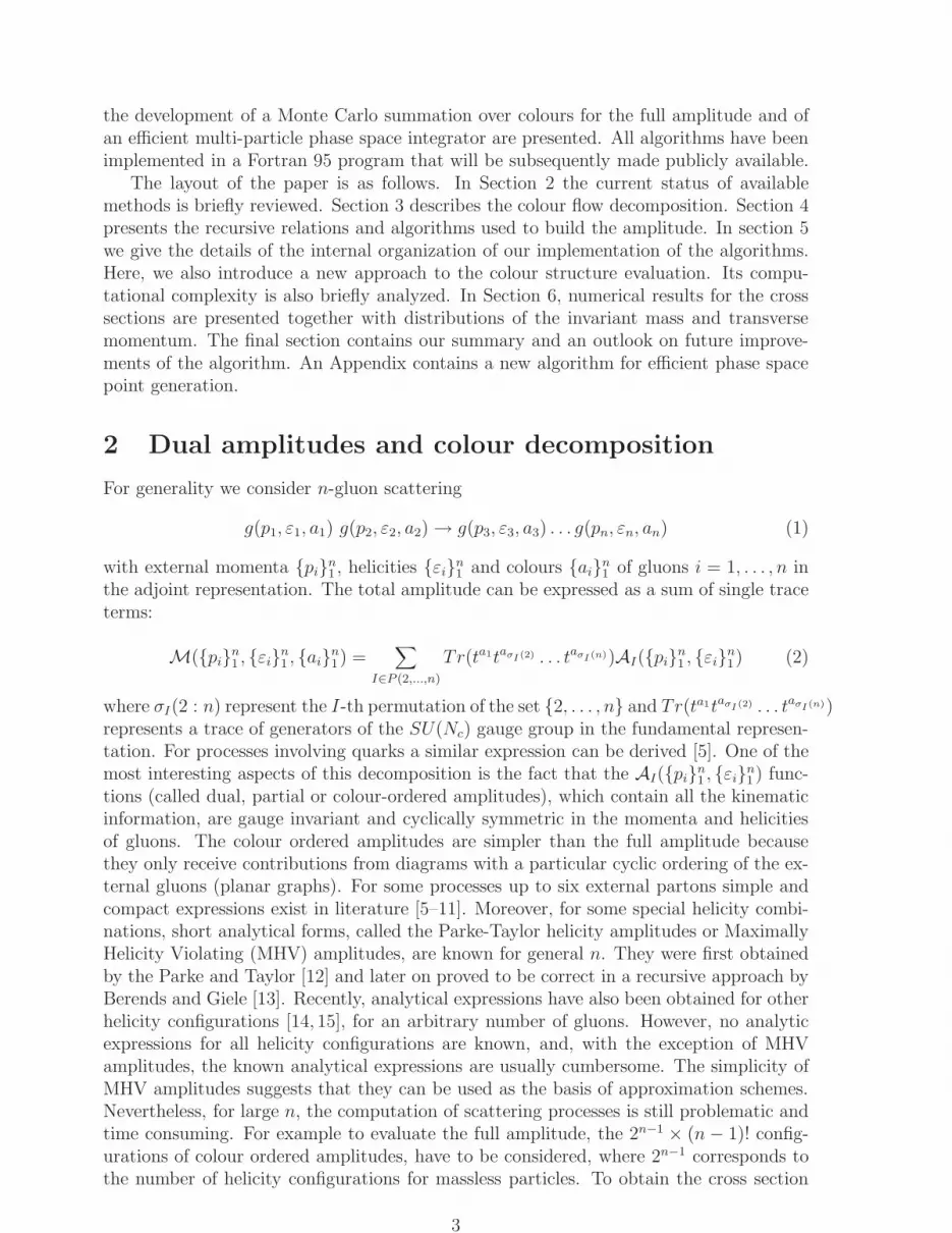
where σI(2 : n) represent the I-th permutation of the set {2, . . . , n} and Tr(ta1taσI (2) . . . taσI (n))represents a trace of generators of the SU(Nc) gauge group in the fundamental represen-tation. For processes involving quarks a similar expression can be derived [5]. One of themost interesting aspects of this decomposition is the fact that the AI({pi}n1 , {εi}n1 ) func-tions (called dual, partial or colour-ordered amplitudes), which contain all the kinematicinformation, are gauge invariant and cyclically symmetric in the momenta and helicitiesof gluons. The colour ordered amplitudes are simpler than the full amplitude becausethey only receive contributions from diagrams with a particular cyclic ordering of the ex-ternal gluons (planar graphs). For some processes up to six external partons simple andcompact expressions exist in literature [5–11]. Moreover, for some special helicity combi-nations, short analytical forms, called the Parke-Taylor helicity amplitudes or MaximallyHelicity Violating (MHV) amplitudes, are known for general n. They were first obtainedby the Parke and Taylor [12] and later on proved to be correct in a recursive approach byBerends and Giele [13]. Recently, analytical expressions have also been obtained for otherhelicity configurations [14, 15], for an arbitrary number of gluons. However, no analyticexpressions for all helicity configurations are known, and, with the exception of MHVamplitudes, the known analytical expressions are usually cumbersome. The simplicity ofMHV amplitudes suggests that they can be used as the basis of approximation schemes.Nevertheless, for large n, the computation of scattering processes is still problematic andtime consuming. For example to evaluate the full amplitude, the 2n−1 × (n− 1)! config-urations of colour ordered amplitudes, have to be considered, where 2n−1 corresponds tothe number of helicity configurations for massless particles. To obtain the cross section

3

from the n-gluon amplitude one has to square and sum over helicity and colour of theexternal gluons. The squared matrix element can be computed by

∑

{ai}n1 {εi}n

1

|M({pi}n1 , {εi}n1 , {ai}n1 )|2 =∑

ε

∑

IJ

AICIJA∗J (3)

where the (n−1)!× (n−1)! dimensional colour matrix can be written in the most generalform as follows:

CIJ =∑

1...Nc

Tr(ta1taσI (2) . . . taσI (n))Tr(ta1taσJ (2) . . . taσJ (n))∗ (4)

Needless to say that the evaluation of this matrix, is by its own a formidable task inthe standard approach.

An important step in the direction of simplification of these calculations has alreadybeen taken by using helicity amplitudes and a better organisation of the Feynman dia-grams [5,10,11,16–19]. A significant simplification in these calculations has been made byintroducing recursive relations [13,20], which express the n-parton currents in terms of allcurrents up to (n− 1) partons. They are based on smaller building blocks which are justcolour ordered vector and spinor currents defined for the off mass shell particles. Extend-ing the recursive approach beyond colour ordered amplitudes, i.e. to the full amplitudein any field theory, is possible. Another approach in this direction based on the so calledALPHA algorithm [21, 22] or the Dyson-Schwinger recursion equations has been devel-oped [23–32], where the multi-parton amplitude can be constructed without referring toindividual Feynman diagrams. In the latter case, apart from the summation over colour inthe colour flow basis, which will be briefly described in the next section, integration overa continuous set of colour variables (as well as flavour) was introduced. This integrationtechnique, however, does not give a straightforward solution for the efficient merging ofthe parton level calculation with the parton shower evolution.

3 The colour flow decomposition

First, let us briefly review the colour approach used in the original version of HELAC [30,31],a multipurpose Monte Carlo generator for multi-particle final states based on the Dyson-Schwinger recursion equations. As was already mentioned, the colour connection or colourflow representation of the interaction vertices was used in this case. This representationwas introduced for the first time in [33] and later studied in e.g. [31, 34]. The advantageof this color representation, as compared to the traditional one is that the colour factorsacquire a much simpler form, which moreover holds for gluon as well as for quark am-plitudes, leading to a unified approach for any tree-order process involving any numberof coloured partons. Additionally, the usual information on colour connections, neededby the parton shower Monte Carlo, is automatically available, without any further cal-culation. In this approach, the gluon field represented as Aa

µ with a = 1, . . . , N2c − 1 is

treated as an Nc×Nc traceless matrix in colour space [29]. The new object (Aµ)AB whereA,B = 1, . . . , Nc can be obtained by multiplying each gluon field by the correspondingtaAB matrix as follow:

(Aµ)AB ≡N2

c −1∑

a=1

taABAaµ. (5)

4

The colour structure of the three gluon vertex is given now by, see Fig. 1.:

∑

ai

fa1a2a3ta1ABt

a2CDt

a3EF = − i

4(δADδCF δEB − δAF δCBδED) (6)

where, on the right hand side only products of δ’s appear. This colour structure showshow the colour flows in the real physical process, where gluons are represented by colour-anticolour states in the colour space, and reflects the fact that the colour remains un-changed on an uninterrupted colour line. For a four gluon vertex the following expression

Figure 1: Colour flows for the three gluon vertex.

Figure 2: Colour flows for the four gluon vertex.

has to be considered:∑

ai

fa1a2xfxa3a4ta1ABt

a2CDt

a3EF t

a4GH (7)

with three permutations of the a1a2a3 indices, which correspond to the six colour flowspresented in Fig.2. Because gluons have N2

c different colour states, described for Nc = 3within the U(3) group we have an additional unphysical neutral U(1) gluon. This neutralgluon does not couple to other gluons as can be easily seen from Eq.(6). It couples onlyto quarks and acts as a colourless particle, see second part of Eq.(8). The colour structureof the quark-antiquark-gluon vertex can be described as follows, see Fig.3:

∑

a

taABtaCD =

1

2(δADδCB −

1

Nc

δABδCD). (8)

5

Figure 3: Colour flows for the qqg vertex.

Let us introduce a more compact notation and associate, to each gluon, a label (i, σi)which refers to the corresponding colour index of previous equations, namely 1 → A,σ1 → B and so on. The use of labels will be explained latter on. With this notation thefirst term of the three gluon vertex is proportional to:

δ1σ2δ2σ3δ3σ1 . (9)

For the same graph with inverted arrows a minus sign and interchanged 2↔ 2 has to beincluded as well. The momentum part of the vertex, V µ1µ2µ3 is still the usual one and inour notation simply given by:

g12(p1 − p2)3 + g23(p2 − p3)

1 + g31(p3 − p1)2. (10)

For the qqg vertex we associate a label (i, 0) for quark and (0, σi) for antiquark. Finallythe four gluon vertex is given by a colour factor proportional to:

δ1σ3δ3σ2δ2σ4δ4σ1 (11)

with six possible permutations, and a Lorentz part, Gµ1µ2µ3µ4 ,

2g13g24 − g12g34 − g14g23 (12)

where all three permutations should be included.To make use of the colour representation described so far, let us assign, to each external

gluon, a label (i, σI(i)), to a quark (i, 0) and to antiquark (0, σI(i))), where i = 1 . . . nand σI(i), I = 1 . . . n! being a permutation of {1 . . . n}. Since all elementary colour factorsappearing in the colour decomposition of the vertices are proportional to δ functions thetotal colour factor can be given by

M({pi}n1 , {εi}n1 , {ci, ai}n1 ) =∑

I=P (2,...,n)

DI AI({pi}n1 , {εi}n1 ) (13)

DI = δ1σI (1)δ2σI (2) . . . δnσI (n) , (14)

The colour matrix defined asCIJ =

∑

IJ

DID†J (15)

6

with the summation running over all colours, 1, . . . , Nc has a very simple representationnow

CIJ = Nm(σI ,σJ)c (16)

where 1 ≤ m(σI , σJ) ≤ n counts how many common cycles the permutations σI andσJ have. The practical implementation of these ideas is straightforward. Given theinformation on the external particles contributing to the process we associate colour labelsof the form (i, σi) depending on their flavour. According to the Feynman rules the higherlevel sub-amplitudes are built up. Summing over all n! colour connection configurations,where n is the number of gluons and qq pairs in the process using the colour matrix CIJ

we get the total squared amplitude. It is worthwhile to note that summing over all colourconfigurations is efficient as long as the number of particles is smaller than O(8). If thenumber of gluons and/or qq pairs is higher than O(8), since the number of colour flowsin general grows like (n − 1)!, it also starts to be problematic from the computationalpoint of view. For multi-colour processes other approaches have to be considered. Thenatural solution would be to replace the summation over all colour connections by aMonte Carlo. However, Monte Carlo summation is not straightforward in the color flowapproach because of the destructive interferences between different colour flows that cangive a negative contribution to the squared matrix element.

In the limit Nc → ∞, only the diagonal terms, I = J , survive, and all O(N−2c )

terms can be safely neglected both in the colour matrix and in the |AI |2. The interfer-ences between different colour flows vanish in this limit. In the so called Leading ColourApproximation (LCA), the squared amplitude for the purely gluonic case is given by

∑

a,ε

|M({pi}n1 , {εi}n1 , {ai}n1 )|2 = Nn−2c (N2

c − 1)∑

ε

∑

I

|AI |2. (17)

The term N2c − 1 instead of N2

c , which of course are equivalent in the limit Nc → ∞,has been kept in order to reproduce the exact results for n = 4 and n = 5. In casewhen qq pairs are present the colour factor Nn−2

c (N2c − 1) is still the same, however

n = ng + nqq in this case, where ng, nqq is the number of gluons and qq pairs respectively.This simplification of the colour matrix speeds up the calculation. Moreover, Monte Carlosummation over colours can now be performed.

4 Dyson-Schwinger recursion relations

Let us now review the recursive relations based on Dyson-Schwinger equations for the cal-culation of partial amplitudes [32]. These equations give recursively the n−point Green’sfunctions in terms of the 1−, 2−,. . ., (n− 1)−point functions. They hold all the informa-tion for the fields and their interactions for any number of external legs and to all orders inperturbation theory. We will concentrate here on the gluon, quark and antiquark recursionrelations, however, in the same way recursive equations for leptons and gauge bosons canbe obtained. The diagrammatic picture behind the recursive relations is actually quitesimple. The tree-level recursive equation can be diagrammatically presented as shown inFig.4. Let p1, p2, . . . , pn represent the external momenta involved in the scattering processtaken to be incoming. In order to write down the recursive relation explicitly, we first de-fine a set of four vectors [Aµ(P ); (A,B)], which describes any sub-amplitudes from whicha gluon with momentum P and colour-anticolour assignment A,B can be constructed.The momentum P is given as a sum of external particles momenta. Accordingly we define

7

a set of four-dimensional spinors [ψ(P ); (A, 0)] describing any sub-amplitude from whicha quark with momentum P and colour A can be constructed and by [ψ(P ); (0, B)] a setof four-dimensional antispinors for antiquark with anticolour B. The Dyson-Schwinger

Figure 4: Recursive equation for an off mass shell gluon of momentum P.

recursion equation for a gluon can be written as follows:

[Aµ(P ); (A,B)] =n∑

i=1

[ δP=piAµ(pi); (A,B)i] (18)

+∑

P=p1+p2

[ (ig) Πµρ V

ρνλ(P, p1, p2)Aν(p1)Aλ(p2)σ(p1, p2); (A,B) = (C,D)1 ⊗ (E,F )2]

−∑

P=p1+p2+p3

[ (g2) Πµσ G

σνλρ(P, p1, p2, p3)Aν(p1)Aλ(p2)Aρ(p3)σ(p1, p2 + p3);

(A,B) = (C,D)1 ⊗ (E,F )2 ⊗ (G,H)3]

+∑

P=p1+p2

[ (ig) Πµν ψ(p1)γ

νψ(p2)σ(p1, p2); (A,B) = (0, D)1 ⊗ (C, 0)2]

where A,B,C,D,E, F,G,H = 1, 2, 3. The rules for merging colour and anticolour of theparticles will be explained in the next section. The V µνλ(P, p1, p2) and Gµνλρ(P, p1, p2, p3)functions are the three- and four- gluon vertices presented in the previous sections andthe symbol σ(p1, p2) is the sign function which takes into account the Fermi sign whentwo identical fermions are interchanged. The exact form of this function can be found inRef. [30, 32]. The sums are over all combinations of p1, p2 or p1, p2, p3 that sum up to P .The propagator of the gluon is given by:

Πµν =−igµν

P 2. (19)

For a quark of momentum P we have, Fig.5:

Figure 5: Recursive equation for an off mass shell quark of momentum P.

8

Figure 6: Recursive equation for an off mass shell antiquark of momentum P.

[ψ(P ); (A, 0)] =n∑

i=1

[ δP=piψ(pi); (A, 0)i] (20)

+∑

P=p1+p2

[ (ig) P Aµ(p1)γµψ(p2)σ(p1, p2); (A, 0) = (B,C)1 ⊗ (D, 0)2]

where P is the propagator

P =iP/

P 2. (21)

Finally for an antiquark, Fig.6:

[ψ(P ); (0, A)] =n∑

i=1

[ δP=piψ(pi); (0, A)i] (22)

+∑

P=p1+p2

[ (ig) ψ(p2)Aµ(p1)γµ Pσ(p1, p2); (0, A) = (B,C)1 ⊗ (0, D)2]

where

P =−iP/P 2

. (23)

In the same spirit, the recursion equations for all leptons and gauge bosons can be writtendown. With this algorithm we can thus compute the scattering amplitude for any initialand final states taking into account particle masses as well. In particular any colourstructure can be assigned to the external legs. Finally this approach has an exponentialgrowth of computational time with the number of external particles instead of the factorialgrowth when Feynman graphs are considered. It can be farther optimised in order toreduce computational complexity by replacing each four gluon vertex by a three particlevertex by introducing the auxiliary field represented by the antisymmetric tensor Ha

µν .This new field has a quadratic term without derivatives and, therefore, has no independentdynamics. The part of the QCD Lagrangian that describes the four gluon vertex

L = −1

4F a

µνFµνa, F a

µν = ∂µAaν − ∂νA

aµ + gfabcAb

µAcν (24)

can be rewritten in terms of the auxiliary field as follows:

L = −1

2Ha

µνHµνa +

1

4Ha

µνFµνa. (25)

A single interaction term of the form HµνaAbµA

cν is left instead of interaction terms rep-

resented by Eq.(24). The recursion for the gluons changes slightly, in fact only for thefour-gluon vertex part. However, we have an additional equation for the auxiliary field:

[Aµ(P ); (A,B)] =n∑

i=1

[ δP=piAµ(pi); (A,B)i] (26)

9

+∑

P=p1+p2

[ (ig) Πµρ V

ρνλ(P, p1, p2)Aν(p1)Aλ(p2)σ(p1, p2); (A,B) = (C,D)1 ⊗ (E,F )2]

+∑

P=p1+p2

[ (ig) Πµσ (gσλgνρ − gνλgσρ) Aν(p1)Hλρ(p2)σ(p1, p2); (A,B) = (C,D)1 ⊗ (E,F )2]

+∑

P=p1+p2

[ (ig) Πµν ψ(p1)γ

νψ(p2)σ(p1, p2); (A,B) = (0, D)1 ⊗ (C, 0)2]

and

[Hµν(P ); (A,B)] =∑

P=p1+p2

[ (ig) (gµλgνρ − gνλgµρ) Aλ(p1)Aρ(p2)σ(p1, p2); (27)

(A,B) = (C,D)1 ⊗ (E,F )2].

A few comments are now in order. First, all calculations were performed in the light conerepresentation and all momenta were taken to be incoming. Second, this new Hµν field hassix components. Additionally, as we can see in Eq.(26) and Eq.(27) the colour structureof this new vertices, remains the same as in case of the three gluon vertex. The number ofthe types of the sub-amplitudes one has to calculate is in general doubled, however theirstructure is much simpler, which saves computational time while the iteration steps areperformed.

After n− 1 steps, where n is the number of particles under consideration, one can getthe total amplitude. The scattering amplitude can be calculated by any of the followingrelations, depending on the process under consideration,

A({pi}n1 , {εi}n1) =

Aµ(Pi)Aµ(pi) where i corresponds to gluonˆψ(Pi)ψ(pi) where i corresponds to quark line

ψ(pi)ψ(Pi) where i corresponds to antiquark line

(28)

wherePi =

∑

j 6=i

pj,

so that Pi + pi = 0. The functions with hat are given by the previous expressions exceptfor the propagator term which is removed by the amputation procedure. This is becausethe outgoing momentum Pi must be on shell. The initial conditions are given by

Aµ(pi) = ǫµλ(pi), λ = ±1, 0

ψ(pi) =

{

uλ(pi) if p0i ≥ 0

vλ(−pi) if p0i ≤ 0

ψ(pi) =

{

uλ(pi) if p0i ≥ 0

vλ(−pi) if p0i ≤ 0

(29)

where the explicit form of ǫµλ, uλ, vλ, uλ, vλ is given in the Ref. [30].

5 Organisation of the calculation

The recursive algorithm presented in the previous section has the advantage that anycolour representation can be used in order to assign colour degrees of freedom to theexternal legs in the process under consideration. It can be used either for colour ordered

10

amplitudes or for the full amplitudes as well. The latter case is in fact the topic of thissection. Moreover, an alternative method for taking into account the colour structureof scattering partons, based on regular colour configuration assignments as compared tocolour flow ones, will be introduced. First, however, the organisation of the calculationwill be explained briefly in order to better describe the general structure. Contrary tothe original HELAC [30, 31] approach, in this new version the computational part consistsof one phase only. This is not optimal for electroweak processes with moderate numberof external particles, but it becomes quite efficient for processes with many particles,especially when only a few species of particles are involved (scalar amplitudes, gluonamplitudes in QCD, etc). The vertices described by the Standard Model Lagrangian areimplemented in fusion rules that dictate the way the subamplitudes, at each level of therecursion relation, will be merged, in order to produce a higher level subamplitude. Incase when a quark is combined with an antiquark, for example, there are three possiblesubamplitudes which describe three different intermediate states incorporated inside thefusion rules, namely γ, Z and g.

Let us now present the colour merging rules which are evaluated iteratively at thesubamplitude level. During each iteration when two particles are combined their corre-sponding colour assignments are combined. We have three possibilities to obtain a gluon(A,B) described by the recursive relation Eq.(26). First, it can be obtained when a quarkwith colour assignment (C, 0) is merged with an antiquark of anticolour (0, D). Second,when two gluons (C,D) and (E,F ) are combined, where A,B,C,D,E, F = 1, 2, 3, andfinally when a gluon and an auxiliary field H are combined. In the last case, the colourstructure of the vertex is identical to the three-gluon vertex. So we end up with thefollowing rules:

(A,B)← (C, 0 )⊗ ( 0, D), (30)

(A,B)← (C,D)⊗ (E,F ). (31)

In the first case the merging occurs according to the rule presented in Eq.(8). and thefollowing gluon can be produced:

(A,B) = (C, 0)⊗ (0, D) = (C,D), if C 6= D. (32)

However, the situation is more complex when a quark and an antiquark have the samecolour and anticolour:

(A,B) = (C, 0)⊗ (0, D) = (1, 1)w1 ⊕ (2, 2)w2 ⊕ (3, 3)w3, if C = D. (33)

with∑

wi = 0. We thus have three possibilities with different weights, which for instanceare w1 = w2 = −1/3, w3 = +2/3 in case C = D = 3.

In the second case, when gluons are combined according to Eq.(6) we have the followingoptions:

(A,B) = (C,D)⊗ (E,F ) = (E,D), if C = F and E 6= D (34)

(A,B) = (C,D)⊗ (E,F ) = (C, F ), if D = E and C 6= F. (35)

Moreover, we have an additional possibility when colours and anticolours of gluons arethe same. One gets, in this case, a gluon in two colour states with different weight:

(A,B) = (C,D)⊗(E,F ) = (C,C)+1⊕(D,D)−1, if C = F E = D and C 6= D. (36)

11

Finally for C = D = E = F the result vanishes identically.To obtain the quark, (A, 0), described by the recursive relation Eq.(20) we have to

combine a gluon with another quark one more time according to the rule presented inEq.(8):

(A, 0) = (B,C)⊗ (D, 0). (37)

We have two possibilities for colour assignment:

(A, 0) = (B,C)⊗ (D, 0) = (B, 0), if C = D, (38)

(A, 0) = (B,C)⊗ (D, 0) = (D, 0), if B = C. (39)

For the antiquark the situation is the same, so we will not elaborate it here.For the qq interactions with γ, Z0,W± or Higgs boson the situation is very simple and

we have only one possibility:

(A, 0)⊗ (0, B) = (0, 0) if A = B. (40)

The sum over colour can be performed in this way by considering all possible colour-anticolour configurations according to the above rules. However, the procedure can befacilitated by Monte Carlo methods where a particular colour-anticolour configurationis randomly selected. As we will see an important gain in computational efficiency isachieved within this framework.

The necessary condition which must be fulfilled, while the particular colour assignmentfor the external coloured particles is chosen, is that the number of colour and anticolourof each type, is the same. Otherwise the particles can not be connected by colour flowlines and the amplitude is identically zero. In the Monte Carlo over colours method onehas to multiply the squared matrix element by a coefficient that counts the number ofnon zero colour configurations.

The number of non zero colour configurations, according to the above mentionednecessary condition is given by

NCC =nq∑

A=0

nq−A∑

B=0

nq−A−B∑

C=0

(

nq!

A!B!C!

)2

δ(nq = A+B + C) (41)

where nq is the total number of colours and A,B,C are the numbers of the colour type 1,2 and 3 respectively. As we already stated, the condition given by Eq.(41) is necessary butnot sufficient. Among this set there are still configurations which do not give contributionsto the total amplitude.

In Tab. 2. and Tab. 3. different numbers of colour configurations in the processunder consideration are presented. In the first column the total number of all colourconfigurations is listed, where NALL

CC = 3nq+nq and nq, nq are the number of quarks andantiquarks respectively and gluons are treated as qq pairs. The second column representsresults for the number of non vanishing colour configurations NCC calculated using Eq.(41).In the next column the ratio NCC/N

ALLCC

is presented. The number of colour configurations(in percentage) inside the NCC set which finally gives rise to non zero amplitudes is shownin the last column. Those numbers NF

CC are evaluated by Monte Carlo. Note that whilethe number of external particles is increased the corresponding number of vanishing colourconfigurations in the third column is decreased, as we can see in Tab. 2.

As far as the summation over the helicity configurations is concerned there are twopossibilities, either the explicit summation over all helicity configurations or a Monte

12

Table 2: The number of colour configurations for the processes with gluons only. NALLCC

corresponds to all possible colour configurations, while NCC corresponds to the numberof colour configurations calculated using formula Eq.(41). In the third column the ratioNCC/N

ALL

CCis presented. In the last column the number of non vanishing colour configura-

tions evaluated by MC NF

CC (in percentage) inside the NCC is shown.

Process NALL

CC NCC NCC/NALL

CC NF

CC (%)

gg → 2g 6561 639 0.0974 59.1gg → 3g 59049 4653 0.0788 68.4gg → 4g 531441 35169 0.0662 77.4gg → 5g 4782969 272835 0.0570 85.0gg → 6g 43046721 2157759 0.0501 90.4gg → 7g 387420489 17319837 0.0447 94.0gg → 8g 3486784401 140668065 0.0403 96.4

Carlo approach. In the latter case, for example for gluon, it is achieved by introducingthe polarisation vector

εµφ(p) = eiφεµ

+(p) + e−iφεµ−(p), (42)

where φ ∈ (0, 2π). By integrating over φ we can obtain the sum over helicities

1

2π

∫ 2π

0dφ εµ

φ(p)(ενφ(p))

∗ =∑

λ=±

εµλ(p)(εν

λ(p))∗.

To determine the cost of computation of the n−point amplitude using the algorithmbased on Dyson-Schwinger equations, one has to count the number of operations [35].

There are

(

nk

)

momenta at each level. The total amount of sub-amplitudes corre-

sponding to those momenta is simply given by:

n−1∑

k=1

(

nk

)

= 2n − 2 (43)

where n is the number of particles involved in the calculation. Moreover one has to counthow many ways exist to split a number of level k to two numbers of levels k1 and k2.The last step is to sum over all levels. The total number of operations that should beperformed in the case when only three-point vertices exist is then

n−1∑

k=1

(

nk

)

k−1∑

l=1

(

kl

)

=n−1∑

k=1

(

nk

)

{2k − 2} = 3n − 3 · 2n + 3. (44)

In the limit n→∞ the number of operations grows like 3n instead of the n! growth in theFeynman graph approach. When the Monte Carlo over colour structures is performed andonly one particular colour configuration is randomly chosen the computational cost of thisalgorithm is given exactly by this expression. Otherwise, this formula must be multipliedby the number of non zero colour configurations for the process under consideration.

13

Table 3: The number of colour configurations for the processes with gluons and one or twoqq pairs. NALL

CCcorresponds to all possible colour configurations, while NCC corresponds to

the number of colour configurations calculated using formula Eq.(41). In the third columnthe ratio NCC/N

ALLCC

is presented. In the last column the number of non vanishing colourconfigurations evaluated by MC NF

CC (in percentage) inside the NCC is shown.

Process NALL

CC NCC NCC/NALL

CC NF

CC (%)

gg → uu 729 93 0.1276 93.5gg → guu 6561 639 0.0974 91.6gg → 2guu 59049 4653 0.0788 92.6gg → 3guu 531441 35169 0.0662 94.6gg → 4guu 4782969 272835 0.0570 96.4gg → 5guu 43046721 2157759 0.0501 97.8gg → 6guu 387420489 17319837 0.0447 98.6

gg → cccc 6561 639 0.0974 99.1gg → gcccc 59049 4653 0.0788 98.8gg → 2gcccc 531441 35169 0.0662 99.0gg → 3gcccc 4782969 272835 0.0570 99.3gg → 4gcccc 43046721 2157759 0.0501 99.6

6 Numerical Results

In this section numerical results for multi-parton production at the LHC are presented.As we will show the Monte Carlo summation over colours, speeds up the calculationsubstantially, compared to the one based on explicit summation, especially for processeswith a large number of colors, i.e. gg → ng with n > 6.

The centre of mass energy was chosen to be√s = 14 TeV. In order to remain far from

collinear and soft singularities and to simulate as much as possible the experimentallyrelevant phase-space regions, we have chosen the following cuts:

pTi> 60 GeV, |yi| < 2.5, ∆Rij > 1.0 (45)

for each pair of outgoing partons i and j. Here pTiand yi are the transverse momentum

and rapidity of a parton respectively defined as:

pTi=√

p2xi

+ p2yi, yi =

1

2ln

(

Ei + pzi

Ei − pzi

)

. (46)

In practice for massless quarks the rapidity is often replaced by the pseudorapidity variableη = − ln tan(θ/2), where θ is the angle from the beam direction measured directly in the

14

Table 4: Results for the total cross section for processes with gluons and quarks with upto two qq pairs. σEXACT corresponds to summation over all possible colour configurations,while σMC corresponds to Monte Carlo summation.

Process σEXACT ± ε (nb) ε (%) σMC ± ε (nb) ε (%)

gg → 2g (0.46572 ± 0.00258)×104 0.5 (0.46849 ± 0.00308)×104 0.6gg → 3g (0.15040 ± 0.00159)×103 1.0 (0.15127 ± 0.00110)×103 0.7gg → 4g (0.11873 ± 0.00224)×102 1.9 (0.12116 ± 0.00134)×102 1.1gg → 5g (0.10082 ± 0.00198)×101 1.9 (0.09719 ± 0.00142)×101 1.5gg → 6g (0.74717 ± 0.01490)×10−1 2.0 (0.76652 ± 0.01862)×10−1 2.4

gg → uu (0.36435 ± 0.00199)×102 0.5 (0.36619 ± 0.00132)×102 0.4gg → guu (0.35768 ± 0.00459)×101 1.3 (0.35466 ± 0.00291)×101 0.8gg → 2guu (0.49721 ± 0.00758)×100 1.5 (0.50053 ± 0.00725)×100 1.4gg → 3guu (0.50598 ± 0.01441)×10−1 2.8 (0.52908 ± 0.01264)×10−1 2.4gg → 4guu (0.51549 ± 0.02017)×10−2 3.9 (0.51581 ± 0.01245)×10−2 2.4

gg → cccc (0.25190 ± 0.00528)×10−2 2.1 (0.24903 ± 0.00373)×10−2 1.5gg → gcccc (0.60196 ± 0.01908)×10−3 3.2 (0.58817 ± 0.00926)×10−3 1.6gg → 2gcccc (0.95682 ± 0.03441)×10−4 3.6 (0.92212 ± 0.02485)×10−4 2.7

detector. The last variable is ∆Rij which is the radius of the cone of the parton definedas

∆Rij =√

(Φi − Φj)2 + (ηi − ηj)2 (47)

with azimuthal angle ∆Φij = Φi − Φj ∈ (0, π)

∆Φij = arccos(

pxipxj

+ pyipyj

pTipTj

)

. (48)

Quarks are treated as massless. All results are obtained with a fixed strong coupling con-stant (αs=0.13). For the parton structure functions, we used CTEQ6L1 PDF’s parametri-sation [36, 37]. For the phase space generation we used the algorithm described in theAppendix, whereas in several cases results were cross checked with

• PHEGAS [38], which automatically constructs mappings of all possible peaking struc-tures of a given scattering process and uses self-adaptive procedures like multi-channel optimisation [39]. PHEGAS exhibits a high efficiency especially in the caseof n(+γ)−fermion production in e+e− collisions as long as the number of externalparticles is smaller than O(8).

15

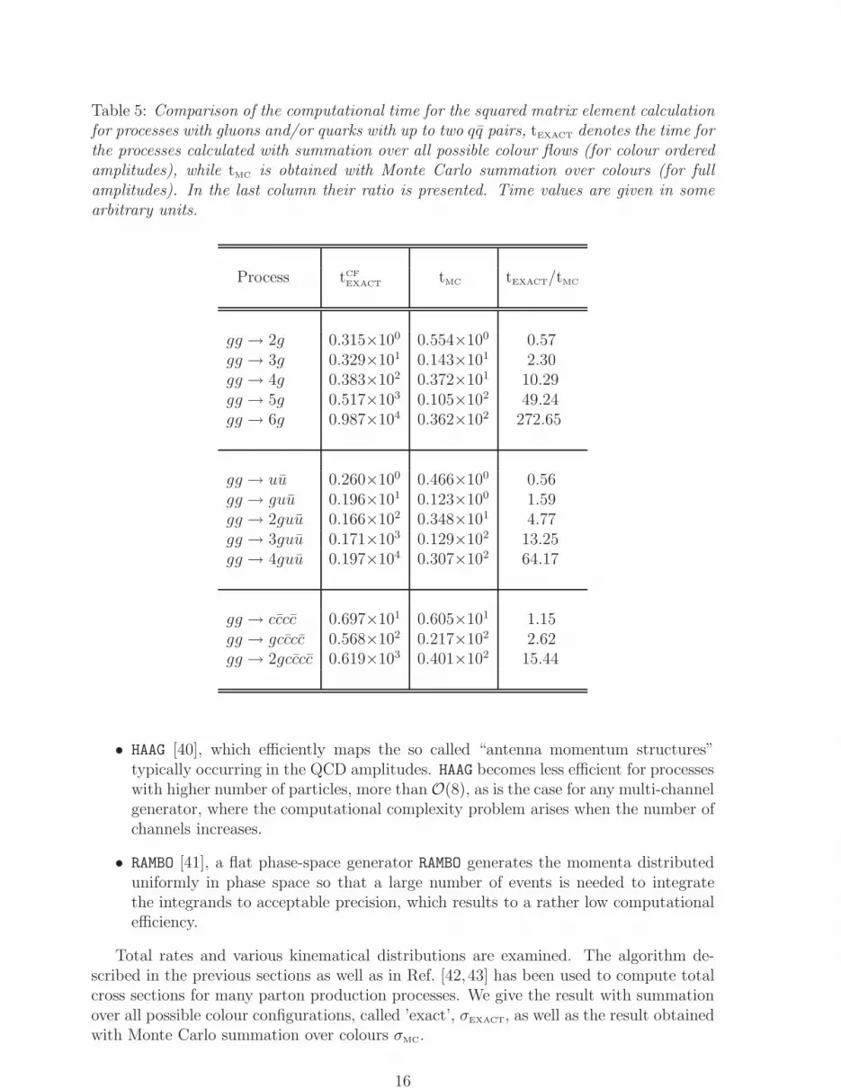
Table 5: Comparison of the computational time for the squared matrix element calculationfor processes with gluons and/or quarks with up to two qq pairs, tEXACT denotes the time forthe processes calculated with summation over all possible colour flows (for colour orderedamplitudes), while tMC is obtained with Monte Carlo summation over colours (for fullamplitudes). In the last column their ratio is presented. Time values are given in somearbitrary units.

Process tCFEXACT

tMC tEXACT/tMC

gg → 2g 0.315×100 0.554×100 0.57gg → 3g 0.329×101 0.143×101 2.30gg → 4g 0.383×102 0.372×101 10.29gg → 5g 0.517×103 0.105×102 49.24gg → 6g 0.987×104 0.362×102 272.65

gg → uu 0.260×100 0.466×100 0.56gg → guu 0.196×101 0.123×100 1.59gg → 2guu 0.166×102 0.348×101 4.77gg → 3guu 0.171×103 0.129×102 13.25gg → 4guu 0.197×104 0.307×102 64.17

gg → cccc 0.697×101 0.605×101 1.15gg → gcccc 0.568×102 0.217×102 2.62gg → 2gcccc 0.619×103 0.401×102 15.44

• HAAG [40], which efficiently maps the so called “antenna momentum structures”typically occurring in the QCD amplitudes. HAAG becomes less efficient for processeswith higher number of particles, more thanO(8), as is the case for any multi-channelgenerator, where the computational complexity problem arises when the number ofchannels increases.

• RAMBO [41], a flat phase-space generator RAMBO generates the momenta distributeduniformly in phase space so that a large number of events is needed to integratethe integrands to acceptable precision, which results to a rather low computationalefficiency.

Total rates and various kinematical distributions are examined. The algorithm de-scribed in the previous sections as well as in Ref. [42,43] has been used to compute totalcross sections for many parton production processes. We give the result with summationover all possible colour configurations, called ’exact’, σEXACT, as well as the result obtainedwith Monte Carlo summation over colours σMC.

16

Table 6: Results for the total cross section for processes with gluons, Z, W± and quarkswith up to qq pairs for the higher number of external partons. σMC corresponds to MonteCarlo summation over colours.

Process σMC ± ε (nb) ε (%)

gg → 7g (0.53185 ± 0.01149)×10−2 2.1gg → 8g (0.33330 ± 0.00804)×10−3 2.4gg → 9g (0.13875 ± 0.00430)×10−4 3.1

gg → 5guu (0.38044 ± 0.01096)×10−3 2.8gg → 3gcccc (0.95109 ± 0.02456)×10−5 2.6gg → 4gcccc (0.81400 ± 0.02583)×10−6 3.2

gg → Zuugg (0.18948 ± 0.00344)×10−3 1.8gg →W+udgg (0.62704 ± 0.01458)×10−3 2.3gg → ZZuugg (0.16217 ± 0.00420)×10−6 2.6gg →W+W−uugg (0.27526 ± 0.00752)×10−5 2.7

dd→ Zuugg (0.38811 ± 0.00569)×10−5 1.5dd→ W+csgg (0.18765 ± 0.00453)×10−5 2.4dd→ ZZgggg (0.99763 ± 0.02976)×10−7 2.9dd→ W+W−gggg (0.52355 ± 0.01509)×10−6 2.9

In case of the explicit summation both colour flow and colour configuration decompo-sition have been used to cross check results. As far as helicity summation is concerned, aMonte Carlo over helicities is applied.

The results presented for the total cross sections, have been obtained for 106 MonteCarlo points passing the selection cuts given by Eg.(45). In the Tab. 4. the results for thetotal cross section for processes with gluons and/or quarks with up to two qq pairs arepresented. All cross sections are in agreement within the error. For the same number ofaccepted events the results with the Monte Carlo summation over colours can be obtainedmuch faster and the error is at the same level compared to the ’exact’ results for the sameprocesses.

In the Tab. 5. a comparison of the computational time for squared matrix elementcalculations for processes with gluons and/or quarks with up to two qq pairs is presented.In each case tEXACT means time obtained for the processes calculated with the summationover all possible colour flows (for colour ordered amplitudes), while tMC is obtained withMonte Carlo summation over colours (for full amplitudes).

17

In the next Tab. 6. the results for the total cross section for processes with gluon,Z, W± and quarks with up to qq pairs for a larger number of external partons are alsopresented.

708090

100

200

300

400

500

600

700800900

1000

0 0.025 0.05 0.075 0.1 0.125 0.15 0.175 0.2 0.225 0.25

dσ/d

z

z

10-1

1

10

10 2

0 0.05 0.1 0.15 0.2 0.25

dσ/d

zz

Figure 7: Distribution in z = |Mone|2/∑all

i |Mi|2, where |Mone|2 is the square matrixelement for one particular colour configuration normalised to the sum of all possible. Theleft-hand side plot corresponds to the gg → 2g process, the right-hand side one to thegg → 3g. Solid line crosses denote summation over all colour configurations whereasdashed, the Monte Carlo summation.

10-5

10-4

10-3

10-2

10-1

1

10

0 100 200 300 400 500 600 700 800

n=4

n=5

n=6

n=7

n=8

dσ/d

Mgg

(nb/

GeV

)

Mgg (GeV)

Figure 8: Invariant mass distribution of 2 gluons in the multigluon 2g → ng process.

In order to demonstrate that the Monte Carlo summation over colours does give thesame information on the colour connection structure of the process, we examine in Fig. 7the distribution of the following variable,

z =|Mone|2

∑alli=1 |Mi|2

(49)

18

10-5

10-4

10-3

10-2

10-1

1

10

0 50 100 150 200 250 300 350 400

n=4

n=5

n=6

n=7

n=8

dσ/d

p T (nb/

GeV

)

pT (GeV)

Figure 9: Transverse momentum distribution of a gluon in the multigluon 2g → ng process.

10-9

10-8

10-7

10-6

10-5

10-4

10-3

10-2

10-1

1

10

0 100 200 300 400 500 600

n=4

n=5

n=6

n=7

n=8

dσ/d

p Tmax

(nb/

GeV

)

pTmax (GeV)

Figure 10: Transverse momentum distribution of the hardest gluon in the multigluon2g → ng process.

where |Mone|2 is the square matrix element for one particular colour connection or colourflow configuration, normalised to the sum of all possible ones. In case of g(1)g(2) →g(3)g(4) process, the following colour flow (1 → 3 → 4 → 2 → 1) has been plotted.This chain of numbers shows how gluons are colour connected with each other. For theg(1)g(2)→ g(3)g(4)g(5) process in the Fig. 7, the colour flow (1→ 5→ 3→ 2→ 4→ 1)is used.

The z−variable distributions can be used in order to extract colour connection infor-mation needed by a parton shower calculation on the event by event basis. The agreementbetween the ’exact’ and MC distributions implies that we will get the same informationon the colour structure of the amplitude and that the merging of parton level calculationwith the parton shower evolution can be safely performed in order to achieve a completedescription of the fully hadronised final states observed in real experiments.

Finally, the distribution of the invariant mass of 2-partons, the transverse momentumdistribution of one parton as well as of the hardest and the softest parton for gg → ng,

19

10-9

10-8

10-7

10-6

10-5

10-4

10-3

10-2

10-1

1

10

0 20 40 60 80 100 120 140 160 180 200

n=4

n=5

n=6

n=7

n=8

dσ/d

p Tmin

(nb/

GeV

)

pTmin (GeV)

Figure 11: Transverse momentum distribution of the softest gluon in the multigluon 2g →ng process.

n = 4, . . . , 8 process is shown in Fig. 8.−Fig. 11. Distributions of the Monte Carlo overcolours clearly demonstrate that this approach performs very well not only at the level oftotal rates but also at the level of differential distributions.

Summary and Outlook

In this work an efficient way for the computation of tree level amplitudes for multi-partonprocesses in the Standard Model was presented. The algorithm is based on the Dyson-Schwinger recursive equations. We discussed how the summation over colour configura-tions can be turned into a Monte Carlo summation, which proved to be more efficient,especially for a large number of coloured partons. Additionally, a set of typical resultsfor total cross sections and differential distributions has been given. Moreover, a new al-gorithm for phase-space generation has been presented and used. The complete packagecan be used to generate, efficiently and reliably, any process with any number of externallegs, for n ≤ 12, in the Standard Model.

Our future interest includes a systematic study of fully hadronic final states in pp andpp collisions which requires the merging of the parton level calculations with parton showerand hadronization algorithms, e.g interfacing our package with codes like PYTHIA [44] orHERWIG [45]. The development of this kind of multipurpose Monte Carlo generators willcertainly be of great interest in the study of TeVatron, LHC and e+e− Linear Colliderdata.

Acknowledgments

Work supported by the Polish State Committee for Scientific Research Grants number1 P03B 009 27 for years 2004-2005 (M.W.). In addition, M.W. acknowledges the MariaCurie Fellowship granted by the European Community in the framework of the HumanPotential Programme under contract HPMD-CT-2001-00105 (“Multi-particle production

20

and higher order correction”). The Greece-Poland bilateral agreement “Advanced com-puter techniques for theoretical calculations and development of simulation programs forhigh energy physics experiments” is also acknowledged.

Appendix

In case of scattering of two hadrons it is useful to describe the final state in terms oftransverse momentum pT , azimuthal angle φ and rapidity y variables. These variablestransform simply under longitudinal boosts which is useful in case of the parton-partonscattering where the centre of mass system is boosted with respect to that of the twoincoming hadrons. In terms of pT , φ and y the four-momentum of a massless particle canbe written as

pµ = (E, px, py, pz) = (pT cosh y, pT cosφ, pT sin φ, pT sinh y) (50)

It is much more natural to express the phase space volume for a system of n particles

Vn =∫

δ4(P −n∑

i=1

pi)n∏

i=1

d4piδ(p2i −m2

i )Θ(p0i ) (51)

using pT , φ and y variables

Vn =∫

δ4(P −n∑

i=1

pi)n∏

i=1

pTidpTi

dyidφi. (52)

To derive the above expression, which lead us to the Monte Carlo algorithm, we followthe method presented in Ref. [41]. We start by defining the phase-space-like object

V0 =∫ ∞

0

(

n∏

i=2

dkTiP (kTi

)

)

∫ 2π

0

(

n∏

i=2

dφi

)

∫ +∞

−∞

(

n∏

i=2

dyi Π(yi)

)

(53)

describing a system of n four momenta that are not constrained by momentum conser-vation but occur with some weight functions P (kTi

), Π(yi) which keeps the total volumefinite. In the next step we have to relate the new variables to the physical ones pTi

, yi

and φi:

V0 =∫ ∞

0

(

n∏

i=2

dkTiP (kTi

)

)

∫ 2π

0

(

n∏

i=2

dφi

)

∫ +∞

−∞

(

n∏

i=2

dyi Π(yi)

)

∫ ∞

0

(

n∏

i=1

dpTiδ(pTi

− xkTi)

)

∫ +∞

−∞

(

n∏

i=2

dyi δ(yi + yi−1 − yi)

)

∫ ∞

0dkT1

∫ 2π

0dφ1 δ(x

n∑

i=2

kTicosφi) δ(x

n∑

i=2

kTisinφi) J1 (54)

∫ ∞

0dx∫ +∞

−∞dy1 δ(x

n∑

i=2

kTicosh yi − E) δ(x

n∑

i=2

kTisinh yi − L) J2.

with the Jacobians J1 and J2:

J1 =

∣

∣

∣

∣

∣

∂(x∑

kTicosφi, x

∑

kTisinφi)

∂(kT1 , φ1)

∣

∣

∣

∣

∣

= x2kT1 (55)

J2 =

∣

∣

∣

∣

∣

∂(x∑

kTicosh yi − E, x

∑

kTisinh yi − L)

∂(x, y1)

∣

∣

∣

∣

∣

=E2 − L2

x. (56)

21

E and L represents the energy and longitudinal parts of the initial two particles. Weproceed with integration where the different arguments of the various δ functions weremanipulated in order to perform the integral

∫ ∞

0

n∏

i=1

dkTiδ(pTi

− xkTi) (57)

∫ +∞

−∞

n∏

i=2

dyi δ(yi + yi−1 − yi). (58)

We are left with

V0 =∫

δ4(P −n∑

i=1

pi)

(

n∏

i=1

pTidpTi

dyidφi

)(

n∏

i=2

P(

pTi

x

)

1

pTi

Π(yi)

)

(E2 − L2)2n

xndx. (59)

We are free to choose the distribution functions so that the total volume is kept finite.The criterion used is to minimize the variance, by taking into account the anticipatedform of the multi-parton matrix elements, so we introduce

P (x) =1

aexp

(−xa

)

, Π(y) =tanh(2η + y) + tanh(2η − y)

8η(60)

where a > 0 and perform the integration over dx

∫ ∞

0

(

n∏

i=2

1

aexp

(−pTi

xa

)

1

pTi

)

1

xndx =

(

n∏

i=2

1

pTi

)(

n∑

i=2

pTi

)−n+1

Γ(n− 1). (61)

We finally arrive at the formula

V0 =∫

δ4(P −n∑

i=1

pi)

(

n∏

i=1

pTidpTi

dyidφi

)

× (62)

(

n∏

i=2

1

pTi

)(

n∑

i=2

pTi

)−n+1

Γ(n− 1)

(

n∏

i=2

Π(yi)

)

(E2 − L2) 2n.

On the other hand if we applied Eq.(60) to the formula Eq.(53) we can find

∫ ∞

0

(

n∏

i=2

dkTi

1

aexp

(

−kTi

a

))

= 1 (63)

∫ +∞

−∞

(

n∏

i=2

dyiΠ(yi)

)

= (8η)n−1 (64)

∫ 2π

0

(

n∏

i=3

dφi

)

= (2π)n−1 (65)

andV0 = (2π · 8η)n−1. (66)

The weight of the event is given by

W =(2π · 8η)n−1

Sn

(67)

22

where

Sn =∫

dpTidyidφi

(

n∏

i=2

1

pTi

)(

n∑

i=2

pTi

)−n+1

Γ(n− 1)

(

n∏

i=2

Π(yi)

)

(E2 − L2) 2n.

In the next step we translate this description into a Monte Carlo procedure and generateindependently n variables kTi

, φi and yi = yi − yi−1 and assuming that φ1 = 0 as well asy1 = 0. Using the symbol ρi to denote a random number uniformly distributed in (0, 1)we do this as follows:

kTi= −a log ρi, i = 2, . . . , n (68)

φi = 2πρi, i = 2, . . . , n (69)

where a is a free parameter. For yi variable we proceed in few steps starting with

Fi = exp(4η(2ρi − 1)) i = 2, . . . , n (70)

where η is a free parameter and

cosh yi =(Fi + 1) sinh 2η

Zi

, sinh yi =(Fi − 1) cosh 2η

Zi

(71)

whereZi =

√

2Fi cosh 4η − (1 + F 2i ). (72)

To complete the description of the algorithm we have to find an expression for kT1 , φ1 andy1 variables. We start by defining the transversal part of the 2, . . . , n system as follows

X ≡n∑

i=2

kTicosφi, Y ≡

n∑

i=2

kTisinφi. (73)

¿From these equations we have the following relations for kT1 and φ1 to be able to describethe total n particle system

cos φ1 = − X

kT1

, sin φ1 = − Y

kT1

(74)

wherekT1 =

√X2 + Y 2. (75)

The total energy and total longitudinal part of the system are represented by

E = kT1 + kT2 cosh(y2) + kT3 cosh(y3 + y2) + . . . (76)

L = kT2 sinh(y2) + kT3 sinh(y3 + y2) + . . . (77)

so y1 is given by

cosh y1 =EE −LL√

E2 − L2√E2 − L2

, (78)

sinh y1 =−LE + EL√

E2 − L2√E2 − L2

, (79)

x =

√

E2 − L2

E2 − L2. (80)

23

Finally to get the final four momenta pµi the following transformations are used:

Ei = xkTicosh yi (81)

pxi = xkTi

cosφi (82)

pyi = xkTi

sinφi (83)

pzi = xkTi

sinh yi. (84)

This completes the description of the algorithm we have to supplemented it with theprescription for the weight of a generated event which is given by Eq.(67).

References

[1] M. A. Dobbs et al., “Les Houches Guidebook to Monte Carlo Generators for HadronCollider Physics”, hep-ph/0403045.

[2] F. Maltoni and T. Stelzer, “Madevent: Automatic event generation with MadGraph”,JHEP 02 (2003) 027, hep-ph/0208156.

[3] F. Krauss, R. Kuhn, and G. Soff, “Amegic++ 1.0: A matrix element generator inC++”, JHEP 02 (2002) 044, hep-ph/0109036.

[4] M. L. Mangano, M. Moretti, F. Piccinini, R. Pittau, and A. D. Polosa, “ALPGEN,a generator for hard multiparton processes in hadronic collisions”, JHEP 07 (2003)001, hep-ph/0206293.

[5] M. L. Mangano and S. J. Parke, “Multiparton amplitudes in gauge theories”, Phys.Rept. 200 (1991) 301.

[6] F. A. Berends, R. Kleiss, P. De Causmaecker, R. Gastmans, and T. T. Wu, “Singlebremsstrahlung processes in gauge theories”, Phys. Lett. B103 (1981) 124.

[7] S. J. Parke and T. R. Taylor, “Perturbative QCD utilizing extended supersymmetry”,Phys. Lett. B157 (1985) 81.

[8] S. J. Parke and T. R. Taylor, “Gluonic two goes to four”, Nucl. Phys. B269 (1986)410.

[9] Z. Kunszt, “Combined use of the calkul method and N=1 supersymmetry to calculateQCD six parton processes”, Nucl. Phys. B271 (1986) 333.

[10] F. A. Berends and W. Giele, “The six gluon process as an example of Weyl-Van derWaerden spinor calculus”, Nucl. Phys. B294 (1987) 700.

[11] M. L. Mangano, S. J. Parke, and Z. Xu, “Duality and multi - gluon scattering”, Nucl.Phys. B298 (1988) 653.

[12] S. J. Parke and T. R. Taylor, “An amplitude for n gluon scattering”, Phys. Rev. Lett.56 (1986) 2459.

[13] F. A. Berends and W. T. Giele, “Recursive calculations for processes with n gluons”,Nucl. Phys. B306 (1988) 759.

24

[14] M. x. Luo and C. k. Wen, “Recursion relations for tree amplitudes in super gaugetheories,” JHEP 0503 (2005) 004, hep-th/0501121.

[15] R. Britto, B. Feng, R. Roiban, M. Spradlin and A. Volovich, “All split helicity tree-level gluon amplitudes,” Phys. Rev. D71 (2005) 105017, hep-th/0503198.

[16] R. Kleiss and W. J. Stirling, “Spinor techniques for calculating pp→W±/Z0 + jets”,Nucl. Phys. B262 (1985) 235.

[17] J. F. Gunion and Z. Kunszt, “Improved analytic techniques for tree graph calculationsand the gg qq lepton antilepton subprocess”, Phys. Lett. B161 (1985) 333.

[18] Z. Xu, D.-H. Zhang, and L. Chang, “Helicity amplitudes for multiple bremsstrahlungin massless nonabelian gauge theories”, Nucl. Phys. B291 (1987) 392.

[19] J. G. M. Kuijf, “Multiparton production at hadron colliders”, Ph.D.Thesis, Univer-sity of Leiden 1991, RX-1335.

[20] W. T. Giele, “Properties and calculations of multiparton processes”, Ph.D.Thesis,University of Leiden 1989, RX-1267.

[21] F. Caravaglios and M. Moretti, “An algorithm to compute born scattering amplitudeswithout Feynman graphs”, Phys. Lett. B358 (1995) 332–338, hep-ph/9507237.

[22] F. Caravaglios, M. L. Mangano, M. Moretti, and R. Pittau, “A new approachto multi-jet calculations in hadron collisions”, Nucl. Phys. B539 (1999) 215,hep-ph/9807570.

[23] E. N. Argyres, R. H. P. Kleiss and C. G. Papadopoulos, Nucl. Phys. B 391 (1993)42.

[24] E. N. Argyres, R. H. P. Kleiss and C. G. Papadopoulos, Nucl. Phys. B 391 (1993)57.

[25] E. N. Argyres, C. G. Papadopoulos and R. H. P. Kleiss, Nucl. Phys. B 395 (1993) 3[arXiv:hep-ph/9211237].

[26] E. N. Argyres, C. G. Papadopoulos and R. H. P. Kleiss, Phys. Lett. B 302 (1993) 70[Addendum-ibid. B 319 (1993) 544] [arXiv:hep-ph/9212280].

[27] E. N. Argyres, R. H. P. Kleiss and C. G. Papadopoulos, Phys. Lett. B 308 (1993)292 [Addendum-ibid. B 319 (1993) 544] [arXiv:hep-ph/9303321].

[28] E. N. Argyres, A. F. W. van Hameren, R. H. P. Kleiss and C. G. Papadopoulos, Eur.Phys. J. C 19 (2001) 567 [arXiv:hep-ph/0101346].

[29] P. Draggiotis, R. H. P. Kleiss, and C. G. Papadopoulos, “On the computation ofmultigluon amplitudes”, Phys. Lett. B439 (1998) 157, hep-ph/9807207.

[30] A. Kanaki and C. G. Papadopoulos, “Helac: A package to compute electroweakhelicity amplitudes”, Comput. Phys. Commun. 132 (2000) 306, hep-ph/0002082.

25

[31] A. Kanaki and C. G. Papadopoulos, “Helac-phegas: Automatic computation of he-licity amplitudes and cross sections”, Published in AIP Conference Proceedings –August 20, 2001 – Volume 583, Issue 1, pp. 169-172 and in Workshop On ComputerParticle Physics: (CPP 2001): Automatic Calculation For Future Colliders, edited byY. Kurihara. Tsukuba, Japan, KEK, 2002. 189p. (KEK-PROCEEDINGS-2002-11),p. 20-25, hep-ph/0012004.

[32] P. D. Draggiotis, R. H. P. Kleiss, and C. G. Papadopoulos, “Multi-jet production inhadron collisions”, Eur. Phys. J. C24 (2002) 447, hep-ph/0202201.

[33] G. ’t Hooft, “A Planar Diagram Theory For Strong Interactions”, Nucl. Phys. B72

(1974) 461.

[34] F. Maltoni, K. Paul, T. Stelzer, and S. Willenbrock, “Color-flow decomposition ofQCD amplitudes”, Phys. Rev. D67 (2003) 014026, hep-ph/0209271.

[35] P. D. Draggiotis, “Exploding QCD - enumeration and computation of QCD pro-cesses”, PhD Thesis, University of Nijmegen 2002.

[36] J. Pumplin et al., “New generation of parton distributions with uncertainties fromglobal QCD analysis”, JHEP 07 (2002) 012, hep-ph/0201195.

[37] D. Stump et al., “Inclusive jet production, parton distributions, and the search fornew physics”, JHEP 10 (2003) 046, hep-ph/0303013.

[38] C. G. Papadopoulos, “Phegas: A phase space generator for automatic cross-sectioncomputation”, Comput. Phys. Commun. 137 (2001) 247, hep-ph/0007335.

[39] R. Kleiss and R. Pittau, “Weight optimization in multichannel Monte Carlo”, Com-put. Phys. Commun. 83 (1994) 141, hep-ph/9405257.

[40] A. van Hameren and C. G. Papadopoulos, “A hierarchical phase space generator forQCD antenna structures”, Eur. Phys. J. C25 (2002) 563, hep-ph/0204055.

[41] R. Kleiss, W. J. Stirling, and S. D. Ellis, “A new Monte Carlo treatment of multi-particle phase space at high-energies”, Comput. Phys. Commun. 40 (1986) 359.

[42] C. G. Papadopoulos and M. Worek, “Multi-particle processes in QCD without Feyn-man diagrams”, Nucl. Instrum. Meth. A559 (2006) 278, hep-ph/0508291.

[43] C. G. Papadopoulos and M. Worek, “Multi-particle processes in the Standard Modelwithout Feynman diagrams”, Acta Phys. Polon. B36 (2005) 3355, hep-ph/0510416.

[44] T. Sjostrand et al., “High-energy-physics event generation with PYTHIA 6.1”, Com-put. Phys. Commun. 135 (2001) 238, hep-ph/0010017.

[45] G. Corcella et al., “HERWIG 6: An event generator for hadron emission reactionswith interfering gluons (including supersymmetric processes)”, JHEP 01 (2001) 010,hep-ph/0011363.

26