
Roadmaps using Gradient Extremal Paths
Ioannis Filippidis and Kostas J. Kyriakopoulos
Abstract— This work proposes a motion planning methodbased on the construction of a roadmap connecting the criticalpoints of a potential field or a distance function. It aims toovercome the limitation of potential field methods due to localminima caused by concave obstacles. The roadmap is incre-mentally constructed by a two-step procedure. Starting from aminimum, adjacent saddle-points are found using a local saddle-point search method. Then, the new saddle-points are connectedto the minima by gradient descent. A numerical continuationalgorithm from the computational chemistry literature is usedto find saddle-points. It traces the valleys of the potentialfield, which are gradient extremal paths, defined as the pointswhere the gradient is an eigenvector of the Hessian matrix.The definition of gradient bisectors is also discussed. Thepresentation conclude simulations in cluttered environments.
I. INTRODUCTION
The problem of motion planning has attracted much atten-tion over the last three decades [1], [2]. Representatives ofdifferent approaches are roadmaps [3], cell decompositions[4], sampling-based methods like RRT, RRT*, PRM* [5] andpotential-field based methods.
Roadmap methods construct a graph whose edges arefeasible paths. Given an initial and final point, they are firstconnected to the roadmap. This reduces the problem to agraph search within the roadmap to connect the entry andexit points. So they are global methods, with the associatedcomputational overhead.
Potential field methods have been pioneered by Khatib[6] and concern the construction of an artificial potentialfield, such that the destination be a minimum. A robotfollowing the potential’s negated gradient is led to the desireddestination. In order to avoid collision with obstacles, thepotential is maximal on the obstacle boundaries.
However, if a local minimum other than the destinationexists, and the robot starts somewhere within its basin ofattraction, then it fails to reach its destination. This originallimitation was overcome by Navigation Functions (NFs)introduced by Koditschek and Rimon [7], which are freeof undesired local minima and exist for any (suff. smooth)Riemannian manifold with boundary. However a construc-tive procedure is available only for sphere worlds [8], [9].Although also applicable to more complex geometries andtopologies [10], [11], e.g., channel surfaces, a converse resultholds for concave obstacles [11].
Ioannis Filippidis is currently with the Control and Dynamical SystemsDept., California Institute of Technology, Pasadena, CA, 91125, USA andwas previously with CSL, NTUA. Kostas J. Kyriakopoulos is with the Con-trol Systems Lab, Department of Mechanical Engineering, National Tech-nical University of Athens, 9 Heroon Polytechniou Street, Zografou 15780,Greece. E-mail: [email protected], [email protected]
The construction of a graph connecting critical points toobtain a roadmap is motivated by results from Morse theoryand was first proposed by Canny [3], using slices of theC-space. Canny and Lin [12] proposed the construction ofroadmaps connecting the critical points of the restrictionof a distance function to slices of the world. Slices offixed direction were used, so the critical points where thosepoints where the distance gradient is normal to the slice.So the freeways of [12] comprise of those points whichhave a fixed gradient direction, the normal to the slices.These are similar to [3] but are constructed in the free spaceinterior, not on the obstacle boundaries. Rimon and Canny[13], [14] extended this work towards using on-line distancemeasurements, without the need for an a priori availabledistance function. A difficulty in the above methods is theremote detection of split and joint points [12], [14] wherethe slice’s topology changes. This issue is not encounteredhere, because the gradient direction is not fixed.
Barraquand et al. [15] proposed the construction of a graphconnecting all critical points of a discrete potential field usingvarious methods. One method is valley-guided motion, wherevalley points are minima of the potential within slices normalto the coordinate axes. This is a discretized version of thefreeways in [12] and is equivalent to the Reduced GradientFollowing (RGF) method [16], [17] reviewed later. Thealgorithm has similar structure to the retraction algorithmproposed in [18]. In contrast, the method used here followsthe direction of least ascent, which can vary and definesexactly the valleys of the potential. It uses a modified versionof the RGF, with an iterative correction of the gradientdirection being searched [19]. During the review process,the authors obtained a copy of [20] where the locus of pointswhere the gradient is a Hessian eigenvector was proposed formotion planning, although no algorithm for the continuouscase was proposed there. Critical point roadmaps have alsobeen studied for coverage tasks using slices of fixed directionin [21], where non-smooth boundaries are treated.
Path planning using a Lagrangian global optimizationmethod under constraints has been proposed in [22], [23]. In[22] planning takes place in a space of dimension equal to thesum of the C-space dimension and the number of obstacles,resulting in a roadmap connecting the maxima and minimaof the potential. The completeness of the algorithm relieson results from [24]. In [25] the construction of a graphconnecting critical points of a distance function in contactspace is discussed, with a discretized implementation.
In the present work we propose the construction of aroadmap comprised of gradient extremal paths (GE), whichare valleys (and ridges) of the potential field. The GEs

connect the minima to saddle-points and maxima, so they canovercome the basins of local minima, although the networkis not always globally connected. To construct each GEsegment (valley), a local saddle-point search method from[19] is used, which is based on a predictor-corrector numer-ical continuation algorithm [26]. Nesting valley constructionwithin graph searching produces the roadmap.
Both Koditschek-Rimon (KR) potential functions (not nec-essarily NFs) and distance functions are used here as scalarfields. KR potentials reduce the search space, by navigating“around” geometric features with sufficient relative convexity[10], [11]. Concave obstacle points can cause local minima,“triggering” the graph search when needed.
The rest of this paper is organized as following: theproblem is defined in § II, local saddle-point searching meth-ods reviewed in § III, the composite navigation algorithmdescribed in § IV and demonstrated though simulations in§ V and conclusions are summarized in § VI.
II. PROBLEM DEFINITIONLet Oi ≜ {x ∈M | βi(x) < 0} where i ∈ I ≜ N∗
≤N areN ∈ N∗ obstacle sets on the C2 n-dimensional Riemannianmanifold M , where βi ∈ C2(M \ Oi,R). When usingpotential fields, then βi should be C2 on a subset densein ∂Oi. If using distance functions and searching thoughobstacles, then βi ∈ C2(M,R). Define the free space asF ≜ M \
∪i∈I Oi and assume it is bounded. By definition
F is closed in M , so F is compact.
A. Distance functions
Distance functions are used to define obstacles and as onetype of scalar field for roadmap construction. Being well-defined within obstacles, they enable searching through them,which can accelerate the search by taking ”short-cuts”. Theirweak point is degeneracy (possibly uncountable critical set)even in simple cases, e.g. for a corridor with parallel sides.The roadmap constructed using a distance function can beused for multiple queries, by connecting each pair of initialcondition and destination to the roadmap.
Constructive Solid Geometry can be performed usingRvachev functions [27], [28] to apply Boolean operationsover the implicit obstacle functions βi, e.g., Fig. 1. Twoalternatives are Rm(u, v) ≜ (u + v ±
√u2 + v2)(u2 +
v2)m2 , Rp(u, v) ≜ u + v ± (up + vp)
1p where m, p even
positive integers and u, v ∈ R. The plus sign correspondsto disjunction and the minus to conjunction. While Rm
functions are Cm everywhere (even at corners u = v =0), they have zero gradient at corners [29]. They must beused if searching though obstacles using a distance field.Rp functions are not differentiable at corner points, butnormalized [29]. In the case of Rp functions with u =βi(x) and v = βj(x), the gradient is ∇xRp = ∇u +
∇v ± (up + vp)1p−1 (
up−1∇u+ vp−1∇v)
and the HessianD2
xRp = (1±upw1p−1)D2u+(1± vp−1w
1p−1)D2v± ((p−
1)up−2vpw1p−1)∇u∇uT± ((p−1)upvp−2w
1p−2)∇v∇vT±
((1− p)up−1vp−1w1p−2) · (∇u∇vT +∇v∇uT), where w ≜
up + vp.
−4
−2
0
2
−1
Fig. 1: Distance function for the 2-dimensional environmentof Fig. 4.
B. Potential fields
In addition to distance functions, the potential field pro-posed by Koditschek and Rimon [7] is used here, de-fined as φ ≜ γd
(γkd+β)
1k
where k ≥ 2, γd ≜ ∥x− xd∥2
and β results using Rvachev operations over the geomet-ric primitives βi. The potential φ can be undesirably flatand is not always defined within obstacles, so the searchshould remain within the free space. For almost all des-tinations there exists some tuning for which φ is Morse[11]. By connecting multiple initial conditions and destina-tions to the roadmap using gradient descent, KRf roadmapscan be used for multiple queries. The gradient of theKoditschek-Rimon potential is ∇ϕ = (γk
d+β)−1k−1(β∇γd−
γd
k ∇β) and the Hessian D2φ = (β(γkd + β)−
1k−1)D2γd +
(− 1kγd(γ
kd + β)−
1k−1)D2β − (γk
d + β)−1k−2
(((k +
1)βγk−1d )∇γd∇γT
d + (− 1k
(1k + 1)γd
)∇β∇βT + (−γk
d +βk )(∇γd∇β
T +∇β∇γTd )
).
C. Problem Statement
The path planning problem comprises of finding a pathin the free space F which connects the initial configurationx(0) of the system to the desired configuration xd. We areinterested in an algorithm which solves the motion planningproblem by constructing a roadmap connecting the minimaand saddle-points of the scalar function used. The algorithmshould also connect the initial configuration x(0) to theroadmap and, depending on the type of scalar function used(β or φ), the final configuration xd as well.
III. LOCAL SADDLE-POINT SEARCH METHODS
Finding saddle-points is inherently more difficult thanminima and the gradient flow cannot be exploited for thispurpose. It has been studied extensively in the literature,however most proposed methods are global (e.g. level-setmethods, nudged elastic band) and many others are to alarge extent heuristic. In motion planning a method usinglocal information would be desired. A standard problemin computational chemistry is the calculation of reactionpaths. These start from reactants and yield products, whichare configurations associated with local minima of potentialenergy, through some saddle point. Local saddle-searchingmethods have been developed for this purpose.

A. Gradient Extremal Paths
Definition 1 (Gradient Extremal [30], [31]): Let f be atwice continuously differentiable function. The locus ofpoints where the gradient is an eigenvector of the Hessianmatrix, i.e., there exists a λ ∈ R such that D2f∇f = λ∇fis called the Gradient Extremal Locus.Geometrically, gradient extremal paths are the valleys, ridges,cirques and cliffs of a scalar function’s graph [31]. Severalequivalent definitions are possible. The gradient extremal isthe locus of points x at which the gradient norm restricted toa level set ∥∇f∥ |f=c attains its minimum or maximum at x(more generally is stationary). This can be proved by show-ing that the defining equation is equivalent to the Lagrangianformulation of the constrained optimization problem of∥∇f∥ over the level set f = c as ∇
{12 ∥∇f∥
2 − λf}= 0,
which implies critical points belong to the gradient extremallocus. An equivalent definition is as the locus of points wherethe gradient flow is geodesic [32]. Moreover, all gradientextremal locus segments start and end at critical points alongthe direction of the eigenvectors of the Hessian matrix [31].
Gradient extremal paths have attracted much attentionover the past 30 years in the theoretical and computationalchemistry literature. One of the first methods of tracing thesecurves was introduced in [33]. However, it suffered fromnumerical difficulties at bifurcation and turning points.
Reduced Gradient Following (RGF) [16] is another saddle-searching method which is closely related to gradient ex-tremal paths. It is equivalent to Branin’s method [17] andimplements a predictor-corrector numerical continuation al-gorithm [26] to follow Newton Trajectories [34], [35]. Theseare the loci of points where the gradient has some desired,fixed direction. The freeways in [12], ridge curves in [13]and valleys in [15] are all equivalent to RGF in a directionfixed and normal to the C-space slices.
The TAngent Search Correction to the RGF (TASC) is amodified version of Reduced Gradient Following proposedby Quapp et. all in [19]. While the predictor step of the RGFsearches for a point with a priori fixed gradient direction,in the TASC the gradient direction searched is iterativelyupdated. In each iteration, the curve tangent of the previousstep becomes the new desired direction for the gradient.The TASC algorithm converges to a valley curve, as provedin [36]. Therefore, it constitutes a more robust methodfor constructing those Gradient Extremal Paths which arevalleys.
We can also define the locus of points where the gradientforms equal angles with each eigenvector of the Hessian (ifon the plane, then it bisects the orthogonal angle formedby each pair of eigenvectors), which we will refer to asgradient bisectors. This new definition is also used here asan alternative to gradient extremal paths and compared tothem in Fig. 2 and the simulations section.
B. Numerical Continuation and Adaptation
A predictor-corrector procedure [26] forms the core of theTASC algorithm, which traces the solutions of a different
−2 −1 0 1 2 3 4 5
−3
−2
−1
0
1
2
3
x0
x
y
minspge
gdna
Fig. 2: Left: Minimal angle θmin of gradient with Hessianeigenvectors. Deep blue curves are gradient extremal paths(θmin = 0) and red curves are gradient bisectors (θmin = π
4 ).Observe that the network of gradient bisectors has betterconnectivity, as compared to gradient extremal paths (in freespace). Right: Critical point roadmap using a distance func-tion and gradient extremal paths for saddle-point searches.
equation in each iteration, instead of a fixed equation (asin RGF). The predictor step in Algorithm 2 increases theintegration step s if the proximity to the solution curve issmaller than the tolerance εexact and s is smaller than theupper threshold smax = cmaxεexact. Then, it moves along thecurrent tangent x′(ti) by s. The corrector step in Algorithm 3reduces the integration step s if s is larger than the lowerthreshold smin = cminεexact. Then, it solves the equationPr∇φ = 0 (where Pr = I − rrT is the matrix projectingon a basis of r⊥) within r⊥ = x′(ti)
⊥, using the correctorconvergence tolerance εcor = s
10 . During the solution itcomputes the Moore-Penrose inverse B† = BT(BBT)−1
of the projected Hessian matrix PrD2φ.
In the TASC Algorithm 1 we define the predictor step sand the tolerance εtol (convergence to saddle-point), εclose(close to the solution curve), εexact (”on” the solution curve).The search starts at a minimum xmin in the direction ofthe eigenvectors of the Hessian matrix, because gradientextremal paths are tangent to them at critical points. A smallperturbation factor cp > εtol
s avoids false convergence tothe initial point within the first iteration. Then, predictor-corrector steps are iteratively performed until convergence.Note that in each iteration the desired gradient direction r isupdated to become equal with the tangent x′ of the previouspredictor step, ensuring convergence to a valley gradientextremal path [36].
For brevity, the algorithm listings do not include someadditional convergence and other tests. The length of theNewton-Raphson step, the gradient norm and Hessian matrixindex are used as convergence criteria. To avoid passingnear a saddle-point without noticing because of too smallεtol, a test is performed of switching from ascending todescending mode. If such a change is detected, then thealgorithm stops and a Newton-Raphson iteration is locallyperformed to improve the saddle-point estimate. When usingφ, which may not be well-defined in obstacles, it is testedwhether x ∈ F .

Algorithm 1 TASC Saddle-Searching Method by GradientExtremal Following [19], [36]
1: procedure TASC(xmin, φ, s, εtol, εclose, εexact, cmin,cmax, cp)
2: r ← eigenvector(D2φ), x(ti)← xmin + cpsr
∥r∥3: x′(ti)← r, stop = 04: while stop = 0 do5: g ← ∇φ (x(ti)), H ← D2φ (x(ti))6: ∆xNR ← −H−1g ▷ Newton-Raphson step7: if ∥∆xNR∥ < εtol then8: stop← 19: end if
10: r ← x′(ti) ▷ Iteratively update gradientdirection searched
11: Pr ← I − rrT ∈ R(n−1)×n ▷ Projection on r⊥
12: u← Prg ∈ R(n−1)
13: B ← PrH ∈ R(n−1)×n ▷ Project Hessian14: x′(ti+1)← null(B) ▷ Kernel of B15: ε← ∥u∥ ▷ Equation satisfaction error16: if ε < εclose then17: [x(ti+1), s] ←PREDICTOR(x(ti), x′(ti), s,
εexact, cmax)18: else19: [x(ti+1), s]←CORRECTOR(s, εtol, cmin)20: end if21: i← i+ 122: end while23: end procedure
Algorithm 2 TASC Predictor
1: procedure PREDICTOR(x(ti), x′(ti), s, εexact, cmax)2: smax ← cmaxεexact3: if ε < εexact and s < smax then4: s← s
√2
5: end if6: x(ti+1)← x(ti) + s x′(ti)
∥x′(ti)∥7: return x(ti+1), s8: end procedure
IV. NAVIGATION ALGORITHM
The path planning Algorithm 4 described starts by agradient descent from x(0) to find a local minimum. Thenusing TASC it follows the four gradient extremals emenatingalong the four Hessian eigenvectors at the minimum. Thisis repeated nested in a depth-first or breadth-first graph-searching algorithm. Duplicate saddle-points are avoided byconsidering x1, x2 as the same saddle-point if ∥x1 − x2∥ <d, some threshold. The RemoveVisited function works sim-ilarly and compares newly discovered critical points toalready known ones. The UpdateAdjacency function addsthe connectivity information between discovered minima andsaddles to the roadmap graph’s adjacency matrix maintained.The convergence test checks if the destination is connectedto the roadmap (or the minimum associated with the desti-
Algorithm 3 TASC Corrector
1: procedure CORRECTOR(s, εtol, cmin)2: smin ← cminεtol3: if s > smin then4: s← s√
25: end if6: εcor ← s
10 ,stop← 07: while stop = 0 do8: g ← ∇φ (x(ti)), H ← D2φ (x(ti)), r ← x′(ti)9: Pr ← I − rrT ∈ R(n−1)×n ▷ Projection on r⊥
10: u← Prg, B ← PrH ∈ R(n−1)×n
11: ε← ∥u∥12: if ε < εcor then13: stop← 114: end if15: B† ← BT(BBT)−1 ▷ Moore-Penrose Inverse16: x(ti)← x(ti)−B†u ▷ Corrector step update17: end while18: x(ti+1)← x(ti)19: return x(ti+1), s20: end procedure
Algorithm 4 Critical Point Graph Construction by Depth-First Search
1: procedure CRITICAL GRAPH(x0, φ, depth, r)2: x(ti)←GRADIENTDESCENT(x0)3: Q← {x(ti)} ▷ Push to queue4: for i = 1 : depth do5: x← pop(Q), Q← Q \ {x} ▷ Pop queue6: {xmin, xsad} ← SEARCHNEXTSADDLES7: xmin ← REMOVEPROXIMATE(xmin, r)8: xmin ← REMOVEVISITED(xmin, xc, r)9: Q← {xmin} ∪Q ▷ Push new minima to queue
10: xc ← xc ∪ {xmin, xsad}11: A← UPDATEADJACENCY(A, xc, r)12: REMOVEPROXIMATE(xc, A, r)13: CONVERGENCETEST14: end for15: end procedure
nation, in case of a distance function).The method’s completeness depends on the global con-
nectivity of the network of gradient extremal paths. Un-fortunately, these are not always globally connected andthe TASC method is attracted to valleys which run alongthe smallest eigenvalue of the Hessian matrix [19], so it isdifficult to converge to steep and transversely shallow saddle-points, also called Don Quixote saddles [37]. Two possibleimprovements are constructing a ridge from a maximum to asaddle-point and the possibility of allowing the search to gothrough obstacles. Bidirectional search is another approachwhich can improve the completeness of the algorithm. De-spite this limitation, the method proves its applicability inthe simulations.
−2 −1 0 1 2 3 4 5
−3
−2
−1
0
1
2
3
x0
xd
x
y
minspge
gdna
−2 −1 0 1 2 3 4 5
−3
−2
−1
0
1
2
3
x0
xd
x
y
minsp
bigdna
Fig. 3: Critical point roadmap on Koditschek-Rimon func-tion. Critical point roadmap of a Koditschek-Rimon functionconstructed using the Gradient Bisector algorithm. Observethat the gradient bisectors achieve improved coverage of thefree space.
−10 −5 0 5
−4
−3
−2
−1
0
1
2
3
4
x
y
minspge
gd
Fig. 4: Navigation in a complicated 2-dimensional envi-ronment using the Koditschek-Rimon potential field andgradient extremal paths for saddle-point searches.
V. SIMULATION RESULTS
This section includes a number of simulations demon-strating the proposed method. The figure abbreviations are:ge (gradient extremal), bi (gradient bisectors), gd (gradientdescent), na (failed search). In Fig. 3-a a 2-dimensional worldwith ellipse obstacles is navigated using the method. Startingfrom the initial condition on the left, the search finds saddle-point passages and then discovers the adjacent basins andtheir associated minima. After a number of iterations, themethod converges to the destination, connecting it to theinitial configuration through the constructed roadmap, whichis comprised of gradient extremal paths and gradient descentpaths. In Fig. 3-b the same world is navigated by gradientbisectors and in Fig. 2-b using gradient extremals on thedistance function. In Fig. 4 another 2-dimensional exampleis shown, where after escaping from the local minimum,the method converges directly to the destination, becausethe potential field reduces the number of minima. For moredetails please refer to [38].
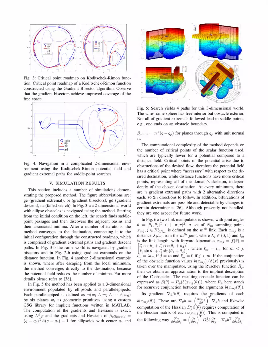
In Fig. 5 the method has been applied to a 3-dimensionalenvironment populated by ellipsoids and parallelepipeds.Each parallelepiped is defined as ¬(w1 ∧ w2 ∧ · · · ∧ w6)by six planes wi as geometric primitives using a customCSG library for implicit functions written in MATLAB.The computation of the gradients and Hessians is exact,using D2φ and the gradients and Hessians of βellipsoid =(q − qc)
TA(q − qc) − 1 for ellipsoids with center qc and
−2−1012345
−4
−3
−2
−1
0
1
2
3
4−1
−0.5
0
0.5
1
1.5
2
2.5
3
3.5
4
y
xd
x
x0
z
min
sp
ge
gd
na
0
1
−3
−2
−1
0
1
xd
x0
min
sp
ge
gd
na
Fig. 5: Search yields 4 paths for this 3-dimensional world.The wire-frame sphere has free interior but obstacle exterior.Not all of gradient extremals followed lead to saddle-points,e.g., one ends on an obstacle boundary.
βplane = nT(q− qp) for planes through qp with unit normaln.
The computational complexity of the method depends onthe number of critical points of the scalar function used,which are typically fewer for a potential compared to adistance field. Critical points of the potential arise due toobstructions of the desired flow, therefore the potential fieldhas a critical point where “necessary” with respect to the de-sired destination, while distance functions have more criticalpoints, representing all of the domain’s skeleton, indepen-dently of the chosen destination. At every minimum, thereare n gradient extremal paths with 2 alternative directionseach, so 2n directions to follow. In addition, bifurcations ofgradient extremals are possible and detectable by changes incertain determinants [26]. Although presently not handled,they are one aspect for future work.
In Fig. 6 a two-link manipulator is shown, with joint anglesθ = [θ1, θ2]
T ∈ [−π, π]2. A set of Nm sampling pointsxmj , j ∈ N∗
≤Nmis defined on the mth link. Each xmj is a
distance λj lm from the mth joint, where λj ∈ (0, 1) and lmis the link length, with forward kinematics xmj = f(θ) =[l′1 cos θ1 + l′2 cos(θ1 + θ2)l′1 sin θ1 + l′2 sin(θ1 + θ2)
], where l′m = lm for m < j,
l′m = λlm if j = m and l′m = 0 if j < m. If the conjunctionof the obstacle function values b(xmj) (β(x) previously) istaken over the manipulator, using the Rvachev function Rp,then we obtain an approximation to the implicit descriptionof the C-obstacles. The resulting obstacle function can beexpressed as β(θ) = Rp(b(xmj(θ))), where Rp here standsfor recursive conjunction between the arguments b(xmj(θ)).
Its gradient ∇θβ(θ) requires the gradients of each
b(xmj(θ)). These are ∇θb =(
∂xmj
∂θ
)T
∇xb and likewisecomputation of the Hessian D2
θβ(θ) requires computation ofthe Hessian matrix of each b(xmj(θ)). This is computed in
the following way ∂2b∂θi∂θj
=(
∂x∂θi
)T
D2xb
∂x∂θj
+∇xbT ∂2x
∂θi∂θj,

−0.5 0 0.5 1 1.5 2 2.5 3
−0.5
0
0.5
1
1.5
x
y
−0.5 0 0.5 1 1.5 2 2.5 3
−0.5
0
0.5
1
1.5
x
y
−2 −1.5 −1 −0.5 0 0.5 1 1.5 2
−3
−2
−1
0
1
2
3
θ1 [rad]
θ2 [
rad
]
x0
xd
min
sp
ge
gd
na
Fig. 6: Right: The C-space distance function for a 2-linkrobotic manipulator, constructed as an approximation ofthe C-space obstacles using a sampling of points on themanipulator and Rvachev conjunction. Two paths are found,comprised of gradient descents and a gradient extremal each.Left: The configuration changes through each path.
where ∂x∂θi
=[∂x1
∂θi∂x2
∂θi
]T. The previous requires the
forward kinematics Jacobian and Hessian, which are
∂x
∂θ=
[−l1 sin θ1 − l2 sin(θ1 + θ2) −l2 sin(θ1 + θ2)l1 cos θ1 + l2 cos(θ1 + θ2) l2 cos(θ1 + θ2)
]∂2x
∂θ21=
[−l1 cos θ1 − l2 cos(θ1 + θ2)−l1 sin θ1 − l2 sin(θ1 + θ2)
]∂2x
∂θ2∂θ1=
∂2x
∂θ1∂θ2=
[−l2 cos(θ1 + θ2)−l2 sin(θ1 + θ2)
]=
∂2x
∂θ22.
For the kinematic Hessian of a general manipulator see [39].More details can be found in [38].
VI. CONCLUSIONS
This paper proposed the combination of exact local valleyfollowing methods of a potential field or distance functionwith graph searching, in order to construct a roadmapconnecting all the minima and saddle points. The method’spotential is demonstrated though a number of case studies.
REFERENCES
[1] J.-C. Latombe, Robot Motion Planning. Kluwer, 1991.[2] S. M. LaValle, Planning Algorithms. Cambridge Uni. Pr., 2006.[3] J. Canny, The complexity of robot motion planning. MIT, 1988.[4] J. Schwartz and M. Sharir, “On the ”piano movers problem. II. general
techniques for computing topological properties of real algebraicmanifolds,” Adv in Appl Math, vol. 4, no. 3, pp. 298 – 351, 1983.
[5] S. Karaman and E. Frazzoli, “Sampling-based algorithms for optimalmotion planning,” Int J of Rob Res, vol. 30, no. 7, pp. 846–894, 2011.
[6] O. Khatib, “Real-time obstacle avoidance for manipulators and mobilerobots,” Int J of Rob Res, vol. 5, no. 1, pp. 90–98, 1986.
[7] D. Koditschek and E. Rimon, “Robot navigation functions on mani-folds with boundary,” Adv in Appl Math, vol. 11, pp. 412–442, 1990.
[8] E. Rimon and D. E. Koditschek, “Exact robot navigation usingartificial potential functions,” IEEE Trans on Rob & Autom, vol. 8,no. 5, pp. 501–518, 1992.
[9] I. Filippidis and K. J. Kyriakopoulos, “Adjustable navigation functionsfor unknown sphere worlds,” in Proc 50th IEEE Conf on Dec & Contr,2011, pp. 4276–4281.
[10] I. F. Filippidis and K. J. Kyriakopoulos, “Navigation functions foreverywhere partially sufficiently curved worlds,” in IEEE Int Conf onRob & Autom, 2012, pp. 2115–2120.
[11] I. Filippidis and K. Kyriakopoulos, “Navigation functions for focallyadmissible surfaces,” in Amer Contr Conf, 2013, (to appear).
[12] J. F. Canny and M. C. Lin, “An opportunistic global path planner,” inProc IEEE Int Conf on Rob & Aut, 1990, pp. 1554–1559.
[13] E. Rimon and J. F. Canny, “Construction of C-space roadmaps fromlocal sensory data-what should the sensors look for?” in Proc IEEEInt Conf Rob & Aut, 1994, pp. 117–123.
[14] E. Rimon, “Construction of C-space roadmaps from local sensory data.what should the sensors look for?” Algorithmica, vol. 17, pp. 357–379,1997.
[15] J. Barraquand, B. Langlois, and J.-C. Latombe, “Numerical potentialfield techniques for robot path planning,” IEEE Trans on Systems, Man& Cybernetics, vol. 22, no. 2, pp. 224 –241, 1992.
[16] W. Quapp, M. Hirsch, O. Imig, and D. Heidrich, “Searching for saddlepoints of potential energy surfaces by following a reduced gradient,”J of Comp Chemistry, vol. 19, no. 9, pp. 1087–1100, 1998.
[17] F. H. Branin, “Widely convergent method for finding multiple so-lutions of simultaneous nonlinear equations,” IBM J of Research &Development, vol. 16, no. 5, pp. 504 –522, 1972.
[18] C. o’Dunlaing, M. Sharir, and C. K. Yap, “Retraction: A new approachto motion-planning,” in Proc 15th annual ACM Symp on Theory ofComputing, 1983, pp. 207–220.
[19] W. Quapp, M. Hirsch, and D. Heidrich, “Following the streambed re-action on potential-energy surfaces: a new robust method,” TheoreticalChemistry Accounts, vol. 105, pp. 145–155, 2000.
[20] J. Barraquand, B. Langlois, and J.-C. Latombe, “Robot motion plan-ning with many degrees of freedom and dynamic constraints,” in 5th
Int Symp on Robotics Research, 1990, pp. 435–444.[21] E. Acar, H. Choset, A. Rizzi, P. Atkar, and D. Hull, “Morse decom-
positions for coverage tasks,” Int J of Rob Research, vol. 21, no. 4,pp. 331–344, 2002.
[22] H. Shashikala, N. Sancheti, and S. Keerthi, “Path planning: an ap-proach based on connecting all the minimizers and maximizers of apotential function,” in Proc IEEE Int Conf on Rob & Aut, 1992, pp.2309–2314.
[23] ——, “A new approach to global optimization using ideas fromnonlinear stability theory,” in Proc IEEE Int Symp on Circuits &Systems, vol. 6, 1992, pp. 2817 –2820 vol.6.
[24] H.-D. Chiang, M. Hirsch, and F. Wu, “Stability regions of nonlinearautonomous dynamical systems,” IEEE Trans on Autom Contr, vol. 33,no. 1, pp. 16 –27, 1988.
[25] T. Allen, J. Burdick, and E. Rimon, “Two-fingered caging of polygonsvia contact-space graph search,” in Proc IEEE Int Conf on Rob &Autom, 2012, pp. 4183 –4189.
[26] E. L. Allgower and K. Georg, Introduction to Numerical ContinuationMethods. SIAM, 2003.
[27] V. Rvachev, Theory of R-functions and Some Applications. Kiev:Naukova Dumka, 1982, (in Russian).
[28] V. Shapiro, “Theory of R-functions and Applications: A Primer,” CSDept, Cornell, Tech. Rep. TR91-1219, 1991.
[29] V. Shapiro and I. Tsukanov, “Implicit functions with guaranteeddifferential properties,” in Proc 5th ACM Symp on Solid Modeling& Appl, 1999, pp. 258–269.
[30] J. Pancir, “Calculation of the least energy path on the energy hyper-surface,” Collection of Czechoslovak Chemical Comm, vol. 40, pp.1112–1118, 1975.
[31] D. K. Hoffman, R. S. Nord, and K. Ruedenberg, “Gradient extremals,”Theoretical Chemistry Accounts, vol. 69, pp. 265–279, 1986.
[32] D. J. Rowe and A. Ryman, “Valleys and fall lines on a Riemannianmanifold,” J of Math Physics, vol. 23, no. 5, pp. 732–735, 1982.
[33] P. Jorgensen, H. Jensen, and T. Helgaker, “A gradient extremal walkingalgorithm,” Theor Chemistry Accounts, vol. 73, pp. 55–65, 1988.
[34] I. Diener, “Trajectory methods in global optimization,” in Handbookof Global Optimization. Kluwer, 1995, pp. 649–668.
[35] M. Hirsch, “Zum reaktionswegcharakter von newtontrajektorien,”Doctor Rerum Naturalium Dissertation, Universitat Leipzig, 2004.
[36] W. Quapp, “A valley following method,” Optimization, vol. 52, no. 3,pp. 317–331, 2003.
[37] P. G. Mezey, “Interrelation between energy-component hypersurfaces,”Chemical Physics Letters, vol. 47, no. 1, pp. 70 – 75, 1977, definitionof ”Don Quixote” and ”Sancho Panza” saddles in p.71.
[38] I. Filippidis and K. Kyriakopoulos, “Gradient extremal roadmaps,”CSL, National Technical Uni Athens, Techical Report, 2012.
[39] A. Hourtash, “The kinematic hessian and higher derivatives,” in ProcIEEE Int Symp on Comp Intel in Rob & Autom, 2005, pp. 169 – 174.
Recommended


