Satisfiability Modulo the Theory of Costs:Foundations and Applications ?

Alessandro Cimatti1, Anders Franzen1, Alberto Griggio2,Roberto Sebastiani2, and Cristian Stenico2

1 FBK-Irst, Trento, Italy2 DISI, University of Trento, Italy

Abstract. We extend the setting of Satisfiability Modulo Theories (SMT) by in-troducing a theory of costs C, where it is possible to model and reason aboutresource consumption and multiple cost functions, e.g., battery, time, and space.We define a decision procedure that has all the features required for the integra-tion withint the lazy SMT schema: incrementality, backtrackability, constructionof conflict sets, and deduction. This naturally results in an SMT solver for thedisjoint union of C and any other theory T .This framework has two important applications. First, we tackle the problem ofOptimization Modulo Theories: rather than checking the existence of a satisfy-ing assignment, as in SMT, we require a satisfying assignment that minimizes agiven cost function. We build on the decision problem for SMT with costs, i.e.,finding a satisfying assigniment with cost within an admissibility range, and pro-pose two algorithms for optimization. Second, we use multiple cost functions todeal with PseudoBoolean constraints. Within the SMT(C) framework, the effec-tively PseudoBoolean constraints are dealt with by the cost solver, while the otherconstraints are reduced to pure boolean reasoning.We implemented the proposed approach within the MathSAT SMT solver, andwe experimentally evaluated it on a large set of benchmarks, also from industrialapplications. The results clearly demonstrate the potential of the approach.

1 Motivations and goals

Important verification problems are naturally encoded as Satisfiability Modulo The-ory (SMT) problems, i.e. as satisfiability problems for decidable fragments of first or-der logic. Efficient SMT solvers have been developed, that combine the power of SATsolvers with dedicated decision procedures for several theories of practical interest.

In many practical domains, problems require modeling and reasoning about re-source consumption and multiple cost functions, e.g., battery, time, and space. In thispaper, we extend SMT by introducing a theory of costs C. The language of the theory ofcosts is very expressive: it allows for multiple cost functions and, for each of these, ar-bitrary Boolean conditions may be stated to result in a given cost increase; costs may be

? A. Cimatti is supported by the European Commission FP7-2007-IST-1-217069 COCONUT.A. Franzen, A. Griggio and R. Sebastiani are supported by SRC under GRC Custom ResearchProject 2009-TJ-1880 WOLFLING, and by MIUR under PRIN project 20079E5KM8 002.

be both lower- and upper-bounded, also depending on Boolean conditions. In the cur-rent paper, we concentrate on the case of Boolean cost functions, where costs are boundby and function of Boolean atoms (including relations over individual variables). Forthe theory of costs, it is possible to define a decision procedure that has all the featuresrequired for the integration within the lazy SMT schema: incrementality, backtracka-bility, construction of conflict sets, and deduction. This naturally results in a solver forSMT(C), and, given the assumption of Boolean cost functions, also in a solver for thedisjoint union of C and any other theory T .

Based on the theory of costs, we propose two additional contributions. First, weextend SMT by tackling the problem of Optimization Modulo Theories: rather thanchecking the existence of a satisfying assignment, as in SMT, we require a satisfyingassignment that minimizes a given cost function. We build on the decision problem forSMT with costs, i.e. finding a satisfying assignment with cost within an admissibilityrange. The optimization problem is then tackled as a sequence of decision problems,where the admissibility range is adapted from one problem to the next. We proposetwo algorithms: one is based on branch-and-bound, where the admissibility range isincreasingly tightened, based on the best valued solution so far. The other one, basedon binary search, proceeds by bisecting the admissible interval, and leveraging under-approximations as well as over-approximations.

Second, we show how to exploit the feature of multiple cost functions to deal withthe well known problem of PseudoBoolean (PB) constraints. The approach can be seenas dealing with PB problems as in an SMT paradigm. The PB constraints are dealt withby the cost solver (as if it were a solver for the theory of PB constraints), while theother constraints are reduced to pure Boolean reasoning. The approach is enabled bythe ability of the cost theory to deal with multiple cost functions. The resulting solutionis very elegant and extremely simple to implement.

We implemented the proposed approach within the MathSAT SMT solver. We ex-perimentally evaluate it on a wide set of benchmarks, including artificial benchmarks(obtained by adding cost functions to the problems in SMT-LIB), real-world (from twodifferent industrial domains) benchmarks, and benchmarks from the PB solver compe-tition. The results show that the approach, despite its simplicity, is very effective: it isable to solve complex case studies in SMT(T ∪ C) and, despite its simplicity, it showssurprising efficiency in some Boolean and PB optimization problems, outperformingthe winners of the most recent comptetition.

This paper is structured as follows. In §2 we present some background. The theoryof costs and the decision procedure are presented in §3. In §4 we show how to tackleoptimization problems. In §5 we show how to encode PseudoBoolean constraints asSMT(C). In §6 we experimentally evaluate our approach. In §7 we discuss some relatedapproaches. In §8 we draw some conclusions and outline directions for future research.The proofs and some possibly-useful material are reported in [8].

2 Background on SMT and SMT solving

Satisfiability Modulo (the) Theory T , SMT(T ), is the problem of deciding the satisfia-bility of (typically) ground formulas under a background theory T . (Notice that T can

2

also be a combination of simpler theories: T def=⋃

i Ti.) We call an SMT(T ) solver anytool able to decide SMT(T ). We call a theory solver for T , T -solver, any tool able todecide the satisfiability in T of sets/conjunctions of ground atomic formulas and theirnegations (T -literals). If the input set of T -literals µ is T -unsatisfiable, then T -solverreturns unsat and the subset η of T -literals in µ which was found T -unsatisfiable; (ηis hereafter called a T -conflict set, and ¬η a T -conflict clause.) if µ is T -satisfiable,then T -solver returns sat; it may also be able to return some unassigned T -literall s.t. {l1, ..., ln} |=T l, where {l1, ..., ln} ⊆ µ. We call this process T -deductionand (

∨ni=1 ¬li ∨ l) a T -deduction clause. Notice that both T - and C-conflict and T -

deduction clauses are valid in T . We call them T -lemmas.We adopt the following terminology and notation. The bijective function T 2B (“T -

to-Boolean”), called Boolean abstraction, maps propositional variables into themselves,ground T -atoms into fresh propositional variables, and is homomorphic w.r.t. Booleanoperators and set inclusion. The symbols ϕ, ψ, φ denote T -formulas, and µ, η denotesets of T -literals. If T 2B(µ) |= T 2B(ϕ), then we say that µ propositionally satisfies ϕwritten µ |=p ϕ. With a little abuse of terminology, we will often omit specifying “theBoolean abstraction of” when referring to propositional reasoning steps, as if these stepswere referred to the ground T -formula/assignment/clause rather than to their Booleanabstraction. (E.g., we say “ϕ is given in input to DPLL” rather “T 2B(ϕ) is...” or “µis a truth assignment for ϕ” rather than “T 2B(µ) is a truth assignment for T 2B(ϕ)”.)This is done w.l.o.g. since T 2B is bijective.

In a lazy SMT(T ) solver the truth assignments for ϕ are enumerated and checkedfor T -satisfiability, returning either sat if one T -satisfiable truth assignment is found,unsat otherwise. In practical implementations, ϕ is given as input to a modified versionof DPLL, and when an assignment µ is found s.t. µ |=p ϕ µ is fed to the T -solver; ifµ is T -consistent, then ϕ is T -consistent; otherwise, T -solver returns the conflict set ηcausing the inconsistency. Then the T -conflict clause ¬η is fed to the backjumping andlearning mechanism of DPLL (T -backjumping and T -learning).

Important optimizations are early pruning and T -propagation: the T -solver is in-voked also on an intermediate assignment µ: if it is T -unsatisfiable, then the procedurecan backtrack; if not, and if the T -solver performs a T -deduction {l1, ..., ln} |=T l,then l can be unit-propagated, and the T -deduction clause (

∨ni=1 ¬li∨ l) can be used in

backjumping and learning. The above schema is a coarse abstraction of the proceduresunderlying all the state-of-the-art lazy SMT tools. The interested reader is pointed to,e.g., [6], for details and further references.

3 Satisfiability Modulo the Theory of Costs

3.1 Modeling cost functions

We extend the SMT framework by adding cost functions. Let T be a first-order theory.We consider a pair 〈ϕ, costs〉, s.t. costs def= {costi}M

i=1 is an array of M integer costfunctions over T and ϕ is a Boolean combination on ground T -atoms and atoms in theform (costi ≤ c) s.t. c is some integer value. 3 We focus on problems in which each

3 Notice that every atom in the form (costi ./ c) s.t. ./ ∈ {=, 6=, <,≤, >,≥} can be expressedas a Boolean combination of constraints in the form (costi ≤ c).

3

costi is a Boolean cost function in the form

costi =∑Ni

j=1 ite(ψij , c

ij1, c

ij2), (1)

s.t., for every i, ψij is a formula in T and ci

j1,cij2 are integer constants values and ite

(term if-then-else) is a function s.t. ite (Aij ,ci

j1,cij2) returns ci

j1 if Aij holds, ci

j2 other-wise. We notice that the problem is very general, and it can express a wide amount ofdifferent interesting problems, as it will be made clear in the next sections.

Hereafter w.l.o.g. we can restrict our attention to problems 〈ϕ, costs〉 in which:

costi =∑Ni

j=1 ite(Aij , c

ij , 0), (2)

for every i, s.t. for every j,Aij is a Boolean literal and 0 < ci

j ≤ cij+1. (Passing from (1)

to (2) is straighforward [8].) We denote by boundimax the value

∑Ni

j=1 cij , for every i.

We notice that we can easily encode (2) into subformulas in the theory of lineararithmetic over the integers (LA(Z)) and hence the whole problem 〈ϕ, costs〉 into aground T ∪LA(Z)-formula, where T and LA(Z) are completely-disjoint theories, andhave it solved by an SMT solver. Unfortunately this technique is inefficient in practice.(An explanation of this fact is reported in [8].) Instead, we cope with this problem bydefining an ad-hoc theory of costs.

3.2 A theory of costs CWe address the problem by introducing a “theory of costs” C consisting in:

– a collection of M fresh variables c1, . . . , cM , denoting the output of the functionscost1,. . . ,costM ;

– a fresh binary predicate BC (“bound cost”), s.t. BC(ci, c) mean “(ci ≤ c)”, ci andc are one of the cost variables and an integer value respectively;

– a fresh ternary predicate IC (“incur cost”), s.t. IC(ci, j, cij) means “ci

j is added toci as jth element in the sum (2)”, ci, j, and ci

j being one of the cost variables, aninteger value denoting the index in the sum (2), and the corresponding integer valuerespectively. 4 We introduce exactly

∑Mi=1Ni distinct atoms IC(ci, j, ci

j), one foreach ci

j in (2).

We call C-atoms all atoms in the form BC(ci, c), IC(ci, j, cij), and C-literals all C-atoms

and their negations. We call a T ∪ C-formula any Boolean combination of ground T -and C-atoms (simply C-formula if T is pure Boolean logic).

Intuitively, the theory of costs allows for modeling domains with multiple costs ci

by means of C- or T ∪ C-formulas. For instance, in the domain of planning for anautonomous rover, different costs may be battery consumption, and elapsed time. Inthe theory of costs, IC statements can be used to state the cost associated to specificpartial configurations. For instance, a specific drilling action may require 5 seconds and20mAh of battery energy,Drill→ (IC(battery, 1, 5)∧ IC(time, 1, 20)), while moving

4 Notice that the index j in IC(ci, j, cij) is necessary to avoid using the same predicate for two

constants cij and ci

j′ with the same value but different indexes j, j′.

4

can have different impact on the available resources: Move → (IC(battery, 2, 20) ∧IC(time, 2, 10)). The BC predicates can be used to state for instance that the achieve-ment of a certain goal G1 should not require more than a certain amount of energy,while another goal should always be completed within a certain time bound and witha certain energy consumption: G1 → BC(battery, 20) and G2 → BC(battery, 20) ∧BC(time, 10). Notice that it is also possible to state lower bounds, e.g. the overall planshould never take less than a certain amount of time.

We consider a generic set µ def= µB ∪ µT ∪ µC s.t. µB is a set of Boolean literals, µTis a set of T -literals, and µC

def=⋃M

i=1 µiC is a set of C-literals s.t., for every i, µi

C is:

µiC

def= {BC(ci, ubi(k)) | k ∈ [1, ...Ki]} ∪ {¬BC(ci, lbi

(m) − 1) |m ∈ [1, ...,Mi]} (3)

∪ {IC(ci, j, cij) | j ∈ J i+} ∪ {¬IC(ci, j, ci

j) | j ∈ J i−}, (4)

where ubi(1), . . . , ubi

(Ki), lbi(1), . . . , lb

i(Mi) are positive integer values, J i+ and J i− are

two sets of indices s.t. J i+ ∩ J i− = ∅ and J i+ ∪ J i− ⊆ {1, . . . , Ni}, and no literal oc-curs both positively and negatively in µ. We say µi

C is total if J i+∪J i− = {1, . . . , Ni},partial otherwise. Notice that every truth assignment µ for a SMT(T ∪ C) formula ϕ isin the form µB ∪ µT ∪ µC described above, s.t. µB, µT and µC are the restriction of µto its Boolean, T - and C-literals respectively.

Let lbimax

def= max({lbi(1), . . . , lb

i(Mi)}) and ubi

mindef= min({ubi

(1), . . . , lbi(Ki)}).

Definition 1. If µiC is total, we say that µi

C is C-consistent if and only if

lbimax ≤

∑j∈Ji+ ci

j ≤ ubimin. (5)

If µiC is partial, we say that µi

C is C-consistent if and only if there exists a total C-consistent superset of µi

C , that is, a C-consistent set µiC∗ in the form

µiC ∪ {IC(ci, j, ci

j) | j ∈ Ki+} ∪ {¬IC(ci, j, cij) | j ∈ Ki−} (6)

s.t. (J i+ ∪Ki+) ∩ (J i− ∪Ki−) = ∅ and (J i+ ∪Ki+ ∪ J i− ∪Ki−) = {1, . . . , Ni}.

Proposition 1. If lbimax > ubi

min, then µiC is C-inconsistent.

Proposition 2. A partial set µiC (3)-(4) is C-consistent if and only if the following two

conditions hold:∑

j∈Ji+ cij ≤ ubi

min (7)

(boundimax −

∑j∈Ji− ci

j)def=

∑j∈{1,...,Ni}\Ji− ci

j ≥ lbimax. (8)

Intuitively, if µiC violates (8), it cannot be expanded into a C-consistent set by adding

positive or negative C-literals. Notice that if µiC is total, then {1, . . . , Ni} \ J i− is J i+,

so that (7) and (8) collapse into the right and left part of (5) respectively. Hereafter wecall

∑j∈Ji+ ci

j the i-th cost of µ, denoted as CostOfi(µ) or CostOfi(µiC), and we call

(boundimax−

∑j∈Ji− ci

j) the maximum possible i-th cost of µ, denoted as MCostOfi(µ)or MCostOfi(µi

C).

5

The notion of C-consistency is extended to the general assignment µ above as fol-lows. We say that µC

def=⋃M

i=1 µiC is C-consistent if and only if µi

C is C-consistent for ev-ery i. We say that µ def= µB∪µT ∪µC is T ∪C-consistent if and only if µT is T -consistentand µC is C-consistent. (Notice that µB is consistent by definition.) A T ∪ C-formula isT ∪ C-satisfiable if and only if there exists a T ∪ C-satisfiable assignment µ defined asabove which propositionally satisfies it.

3.3 A decision procedure for the theory of costs: C-solver

We add to the SMT(T ) solver one theory solver for the theory of costs C (C-solverhereafter). C-solver takes as input a truth assignment µ def= µB ∪ µT ∪ µC selecting onlythe C-relevant part µC

def=⋃M

i=1 µiC , and for every i, it checks whether µi

C is C-satisfiableaccording to Propositions 1 and 2. This works as follows:

1. if lbimax > ubi

min, then C-solver returns unsat and the C-conflict clause

BC(ci, lbimax − 1) ∨ ¬BC(ci, ubi

min); (9)

2. if CostOfi(µiC) > ubi

min, then C-solver returns unsat and the C-conflict clause

¬BC(ci, ubimin) ∨∨

j∈Ki+ ¬IC(ci, j, cij) (10)

where Ki+ is a minimal subset of J i+ s.t.∑

j∈Ki+ cij > ubi

min;3. if MCostOfi(µi

C) < lbimax, then C-solver returns unsat and the C-conflict clause

BC(ci, lbimax − 1) ∨∨

j∈Ki− IC(ci, j, cij) (11)

where Ki− is a minimal subset of J i− s.t.∑

j∈Ki− cij < lbi

max;

If neither condition above is verified for every i, then C-solver returns sat, and thecurrent values of ci (i.e., CostOfi(µ)) for every i. In the latter case, theory propagationfor C (C-propagation hereafter) can be performed as follows:

4. every unassigned literal BC(ci, ubi(r)) s.t. ubi

(r) ≥ ubimin and every unassigned

literal ¬BC(ci, lbi(s) − 1) s.t. ubi

(s) ≤ lbimax can be returned (“C-deduced”). It

is possible to build the corresponding C-deduction clause by applying step 1. toµiC ∪ {BC(ci, ubi

(r))} and µiC ∪ {¬BC(ci, lbi

(s) − 1)} respectively;5. if CostOfi(µi

C) ≤ ubimin but CostOfi(µi

C ∪ {IC(ci, j, cij)}) > ubi

min for somej 6∈ (J i+ ∪ J i−), then ¬IC(ci, j, ci

j) is C-deduced. It is possible to build the corre-sponding C-deduction clause by applying step 2. to µi

C ∪ {IC(ci, j, cij)};

6. if MCostOfi(µiC) ≥ lbi

max but MCostOfi(µiC ∪ {¬IC(ci, j, ci

j)}) < lbimax for some

j 6∈ (J i+ ∪ J i−), then IC(ci, j, cij) is C-deduced. It is possible to build the corre-

sponding C-deduction clause by applying step 3. to µiC ∪ {¬IC(ci, j, ci

j)}.

C-solver can be easily implemented in order to meet all the standard requirementsfor integration within the lazy SMT schema. In particular, it can work incrementally,

6

by updating CostOfi(µ) and MCostOfi(µ) each time a literal in the form IC(ci, j, cij) or

¬IC(ci, j, cij) is added to µ. Detecting the C-inconsistency inside C-solver is computa-

tionally very cheap, since it consists in performing only one sum and one comparisoneach time a C-literals is incrementally added to µC . (Thus, is O(1) for every incrementalcall.) The cost of performing C-propagation is linear in the number of literals propa-gated (in fact, it suffices to scan the IC(ci, j, ci

j) literals in decreasing order, until noneis C-propagated anymore).

3.4 A SMT(T ∪ C)-solver

A SMT(T ∪ C)-solver can be implemented according to the standard lazy SMT archi-tecture. Since the theories T and C have no logic symbol in common (C does not haveequality) so that they do not interfere to each other, T -solver and C-solver can be runindependently. In its basic version, a SMT(T ∪ C) solver works as follows: an inter-nal DPLL solver enumerates truth assignments propositionally satisfying ϕC and bothC-solver and T -solver are invoked on on each of them. If both return sat, then the prob-lem is satisfiable. If one of the two solvers returns unsat and a conflict clause C, thenC is used as a theory conflict clause by the rest of the SMT(T ∪ C) solver for theory-driven backjumping and learning. The correctness an completeness of this process is adirect consequence of that of the standard lazy SMT paradigm, of Proposition 3 and ofthe definitions of C- and T ∪ C-consistency. As with plain SMT(T ), the SMT(T ∪ C)solver can be enhanced by means of early-pruning calls to C-solver and C-propagation.

4 Optimization Modulo Theories via SMT(T ∪ C)

In what follows, we consider the problem of finding a satisfying assignment to anSMT(T ) formula which is subject to some bound constraints to some Boolean costfunctions and such that one Boolean cost function is minimized. We refer to this prob-lem as Boolean Optimization Modulo Theory (BOMT). We first address the decisionproblem (§4.1) and then the minimization problem (§4.2).

4.1 Addressing the SMT(T ) cost decision problem

An SMT(T ) cost decision problem is a triple 〈ϕ, costs, bounds〉 s.t. ϕ is a T -formula,costs are in the form (2), and bounds

def= {〈lbi, ubi〉}Mi=1, where lbi, ubi are integer

values s.t. 0 ≤ lbi ≤ ubi ≤ boundimax. We call lbi, ubi and [lbi, ..., ubi] the lower

bound, the upper bound and the range of costi respectively. (If some of the lbi’s andubi’s are not given, we set w.l.o.g. lbi = 0 and ubi = boundi

max.)We encode the decision problem 〈ϕ, costs, bounds〉 into the SMT(T ∪ C)-satisfiability

problem of the following formula:

ϕCdef= ϕ ∧∧M

i=1

(BC(ci, ubi) ∧ ¬BC(ci, lbi − 1) ∧∧Ni

j=1(Aij ↔ IC(ci, j, ci

j))).(12)

Proposition 3. A decision problem 〈ϕ, costs, bounds〉 has a solution if and only if ϕCis T ∪C-satisfiable. In such a solution, for every i, the value of ci is CostOfi(µ), µ beingthe T ∪ C-satisfiable truth assignment satisfying ϕC .

7

1. int IncLinearBOMT(ϕC,c1)2. mincost = +∞; bound = ub1;3. do4. 〈status, cost〉 = IncrementalSMTT ∪C(ϕC, BC(c1, bound));5. if (status==sat)6. then {7. ϕC = ϕC ∧ BC(c1, bound); //activates learned C-lemmas8. mincost = cost;9. bound = cost-1; }

10. while (status==sat);11. return mincost;

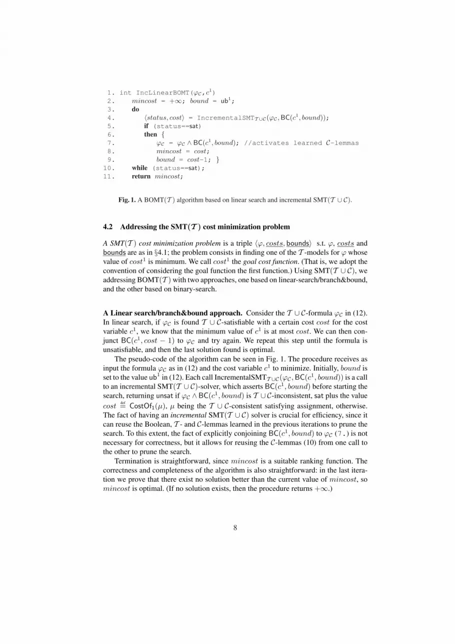
Fig. 1. A BOMT(T ) algorithm based on linear search and incremental SMT(T ∪ C).

4.2 Addressing the SMT(T ) cost minimization problem

A SMT(T ) cost minimization problem is a triple 〈ϕ, costs, bounds〉 s.t. ϕ, costs andbounds are as in §4.1; the problem consists in finding one of the T -models for ϕ whosevalue of cost1 is minimum. We call cost1 the goal cost function. (That is, we adopt theconvention of considering the goal function the first function.) Using SMT(T ∪ C), weaddressing BOMT(T ) with two approaches, one based on linear-search/branch&bound,and the other based on binary-search.

A Linear search/branch&bound approach. Consider the T ∪ C-formula ϕC in (12).In linear search, if ϕC is found T ∪ C-satisfiable with a certain cost cost for the costvariable c1, we know that the minimum value of c1 is at most cost. We can then con-junct BC(c1, cost − 1) to ϕC and try again. We repeat this step until the formula isunsatisfiable, and then the last solution found is optimal.

The pseudo-code of the algorithm can be seen in Fig. 1. The procedure receives asinput the formula ϕC as in (12) and the cost variable c1 to minimize. Initially, bound isset to the value ub1 in (12). Each call IncrementalSMTT ∪C(ϕC ,BC(c1, bound)) is a callto an incremental SMT(T ∪ C)-solver, which asserts BC(c1, bound) before starting thesearch, returning unsat if ϕC ∧BC(c1, bound) is T ∪ C-inconsistent, sat plus the valuecost

def= CostOf1(µ), µ being the T ∪ C-consistent satisfying assignment, otherwise.The fact of having an incremental SMT(T ∪ C) solver is crucial for efficiency, since itcan reuse the Boolean, T - and C-lemmas learned in the previous iterations to prune thesearch. To this extent, the fact of explicitly conjoining BC(c1, bound) to ϕC (7.) is notnecessary for correctness, but it allows for reusing the C-lemmas (10) from one call tothe other to prune the search.

Termination is straightforward, since mincost is a suitable ranking function. Thecorrectness and completeness of the algorithm is also straightforward: in the last itera-tion we prove that there exist no solution better than the current value of mincost, somincost is optimal. (If no solution exists, then the procedure returns +∞.)

8

1. int IncBinaryBOMT(ϕC,c1)2. lower = lb1; upper = ub1;3. mincost = +∞; guess = ub1;4. do5. 〈status, cost〉 = IncrementalSMTT ∪C(ϕC, BC(c1, guess));6. if (status==sat)7. then {8. ϕC = ϕC ∧ BC(c1, guess); // activates learned C-lemmas9. mincost = cost;

10. upper = cost-1; } // more efficient than guess-111. else {12. ϕC = ϕC ∧ ¬BC(c1, guess); // activates learned C-lemmas13. lower = guess +1; }14. guess = b(lower + upper)/2c;15. while (lower ≤ upper);16. return mincost;

Fig. 2. A BOMT(T ) algorithm based on binary search and incremental SMT(T ∪ C).

A binary-search approach. A possibly faster way of converging on the optimal solu-tion is binary search over the possible solutions. Instead of tightening the upper boundwith the last solution found, we keep track of the interval of all possible solutions[lower, upper], and we proceed bisecting such interval, each time picking a guess asb(lower + upper)/2c.

The pseudo-code of this algorithm can be seen in Fig. 2. As before, the proce-dure receives as input ϕC and c1. [lower, upper] is initialized to [lb1, ub1], mincostto +∞ and guess to ub1; each call IncrementalSMTT ∪C(ϕC ,BC(c1, bound)) eitherreturns sat plus the value cost def= CostOf1(µ), or it returns unsat. In the first case,the range is restricted to [lower, cost − 1] (10.), in the latter to [guess + 1, upper](13.). (Notice that, unlike with standard binary search, restricting to [lower, cost− 1]rather than to [lower, guess − 1] allows for exploiting the cost information to furtherrestrict the search.) Moreover, in the first case BC(c1, bound) is conjoined to ϕC (8.),¬BC(c1, bound) in the latter (12.), which allows for reusing the previously-learnedC-lemmas (10) end (11) respectively to prune the search.

Termination is straightforward, since upper − lower is a suitable a ranking func-tion. Correctness and completeness are similarly obvious, since the interval of possiblesolutions will always contain the optimal solution.

5 PseudoBoolean and MAX-SAT/SMT as SMT(C)/SMT(T ∪ C)

The PseudoBoolean (PB) problem can be defined as the problem:

minimizeN1∑

j=1

c1jA

1j under the constraints {

Ni∑

j=1

cijA

ij ≥ lbi | i ∈ [2, ...,M ]}(13)

9

whereA1j are Boolean atoms,Ai

j Boolean literals, and cj , cij , lb

i positive integer values.This is an extension of the SAT problem which can efficiently express many problemsof practical interest.

The SMT (C) problem is closely related to the PB problem, in fact they are equallyexpressive. First, we notice that

∑j ci

jAij can be rewritten as

∑j ite(A

ij , c

ij , 0), s.t.

we immediately see that the PB problem (13) is a subcase of the BOMT(T ) problem of§4.2 where T is plain Boolean logic, and as such it can be solved using the SMT(T ∪ C)encoding in (12) and the SMT(T ∪ C)-based procedures in §4.2.

For solving PB problems by translation into SMT (C) in practice, the above trans-lation can be improved. As an example, PB constraints of the form

∑j A

ij ≥ 1 can

be translated into the single propositional clause∨

j Aij . In general, it may be advanta-

geous to translate PB constraints into propositional clauses when the number of result-ing clauses is low. See for instance [10] for some possibilities.

Proposition 4. For every SMT (C) instance, there exists a polynomial-time translationinto an equivalent instance of the PB problem

In the Weighted Partial Max-SMT(T ) problem, in a CNF T -formula φ def= φh ∧ φs

each clause Cj in φs is tagged with a positive cost value cj , and the problem consistsin finding a T -consistent assignment µ which propositionally satisfies φh and maxi-mizes the sum

∑j s.t.µ|=pCj

cj (that is, minimizes∑

j s.t.µ 6|=pCjcj). The problem is

not “Weighted” iff cij = 1 for every j, and it is not “Partial” iff φh is the empty set

of clauses; the [Weighted] [Partial] Max-SAT problem is the [Weighted] [Partial] Max-SMT(T ) problem where T is plain Boolean logic.

A Weighted Partial Max-SMT(T ) problem (and hence all its subcases describedabove) can be encoded into a SMT(T ) cost minimization problem 〈ϕ, costs, bounds〉s.t. ϕ def= φh ∧

∧j(Cj ∨ Ai

j), costsdef= {cost1} = {∑j ite(A

ij , c

ij , 0)} and bounds

def={〈0,∑j ci

j〉}, which can be addressed as described in §4.2.

Vice versa, a SMT(T ) cost minimization problem 〈ϕ, costs, bounds〉 s.t. costs def={cost1} = {∑j ite(A

1j , c

ij , 0)} and bounds

def= {}, can be encoded into a Weighted

Partial Max-SMT(T ) problem φdef= φh ∧ φs where φh

def= ϕ and φsdef=

∧j(¬A1

j ) s.t.each unit-clause (¬A1

j ) is tagged with the cost cij .

6 Empirical evaluation

The algorithms described in the previous sections have been implemented within theMATHSAT SMT solver. In order to demonstrate the versatility and the efficiency of ourapproach, we have tested MATHSAT in several different scenarios: BOMT(T ), Max-SMT, Max-SAT, and PseudoBoolean optimization.

6.1 Results on Max-SMT

In the first part of our experiments, we evaluate the behaviour of MATHSAT on prob-lems requiring the use of a combination of C and another theory T . For this evaluation,

10

we have collected two kinds of benchmarks. First, we have randomly-generated someMax-SMT problems, 5 starting from standard SMT problems taken from the SMT-LIB.The second group of benchmarks comes from two real-world industrial case studies.These are the case studies that actually prompted us towards this research, becausea plain encoding in SMT without costs resulted in unacceptable performance. Inter-estingly, although the application domains are very different, all the problems can bethought of as trying to find optimal displacement for some components in space. Un-fortunately, we can not disclose any further details.

As regards the comparison with other systems, to the best of our knowledge thereare two other SMT solvers that support Max-SMT, namely YICES [9] and BARCEL-OGIC [13], which were therefore the natural candidates for comparison. Unfortunatelyhowever, it was not possible to obtain from the authors a version of BARCELOGIC withsupport for optimization, so we had to exclude it from our analysis.

We have performed experiments on weigthed Max-SMT and partial weighted Max-SMT problems. For weighted Max-SMT, we have generated benchmarks by combiningn independent unsatisfiable CNF formulas in the SMT-LIB (for n = 2 and n = 3) andassigning random weights to each clause. In order to obtain partial weighted Max-SMTinstances, instead, we have first generated random BOMT(T ) problems by assigningrandom costs to a subset of the atoms (both Boolean and T -atoms) of some satisfi-able formulas in the SMT-LIB, and then encoded the BOMT(T ) problems into partialweighted Max-SMT ones, as descrbed in §5. The same encoding into partial weightedMax-SMT was used also to convert the BOMT(T ) instances coming from the industrialcase studies.

We ran MATHSAT using both binary and linear search for optimization, and com-pared it with YICES. All the experiments have been performed on 2.66Ghz Intel Xeonmachines with 6Mb of cache, running Linux. The time limit was set to 300 seconds,and the memory limit to 2Gb.

The results for problems generated from SMT-LIB instances are reported in Table 1.For each solver, the table lists the number of instances for which the optimal solutionwas found (the total number of instances was 200), the number of instances for whichthe given solver was the only one to find the optimal solution, and the total and averageexecution times on the solved instances. From the results, we can see that binary searchoutperforms linear search for this kind of problems. This is true in particular on the firstgroup of benchmarks, where binary search can find the optimum for more than twice asmany instances as linear search. In both cases, moreover, MATHSAT outperforms alsoYICES, both in number of optimal solutions found and in execution time.

We also measured the overhead of performing optimization on these instances com-pared to solving the decision problem given the known optimal bound. For partial Max-SMT and binary search the mean was 9.5, the median 4.1 and the maximal ratio 49.6,meaning that solving the optimization problem took on average 9.5 times as long as de-termining that the optimal solution is indeed a solution. Similarly, for partial Max-SMTand linear search the mean of the ratio was 45.8, the median 24.3 and the maximal 222.3showing that the overhead in linear search can be considerable. In the weighted partial

5 As observed in §5 BOMT(T ) with a single cost function is equivalent to weighted partialMax-SMT, and therefore we only refer to Max-SMT here.

11

Category Solver Optimum Unique Time Mean Median

Weighted MATHSAT-binary 56 6 4886.59 87.26 68.38Max-SMT YICES 47 3 5260.67 111.92 86.21

MATHSAT-linear 23 0 4777.45 207.71 251.00

Weighted partial MATHSAT-binary 206 1 1462.98 7.10 2.45Max-SMT MATHSAT-linear 206 1 2228.39 10.81 4.02(BOMT(T )) YICES 195 0 3559.53 18.25 3.19

Table 1. Performance on Max-SMT and BOMT(T ) problems. For each category, the solversare sorted from “best” to “worst”. Optimum is the number of instances where the optimum wasfound, and Unique is the number of optimal solutions found by a the given solver only. Timeis the total execution time in seconds for all instances where an optimum was found. Mean andmedian is the mean and median of those times.

Max-SMT problem the overhead was slightly lower. Using binary search the mean was2.6, the median 3.4 and the maximal 22.1. Using linear search we get a mean of 4.4, amedian of 5.9 and a maximal of 54.

Finally, we compared MATHSAT-linear, MATHSAT-binary and YICES on the twoindustrial case studies we had. In the first one, all three solvers could find the optimumon all the 7 instances of the set. YICES turned out to be the fastest, with a median runtime of 0.5 seconds. The median time for MATHSAT-binary was of 1.54 seconds, andthat of MATHSAT-linear of 64.84 seconds. In the second case study, composed of twoinstances, however, the outcome was the opposite: MATHSAT-linear and MATHSAT-binary could compute the optimum for both instances in approximately the same time,with the former being slightly faster (about 35 seconds for the easiest problem for bothsolvers, about 370 and 405 seconds respectively for the hardest). Yices, instead, couldnot compute the optimum for the hardest problem even with a timeout of 30 minutes(taking about 11 seconds on the easiest instead).

6.2 Results on Max-SAT

We have also performed comparisons with several Max-SAT solvers from the 2009Max-SAT Evaluation [1]. For each of the three industrial categories containing pureMax-SAT, partial Max-SAT and partial weighted Max-SAT respectively we have cho-sen 100 instances randomly (in the case of partial weigted Max-SAT, we chose all 80instances). We chose 3 solvers (MsUncore [11], SAT4J [4], and Clone [14]) participat-ing in the 2009 competition that were readily available together with the YICES SMTsolver [9], and ran each of them on all instances supported by that particular solver. Werun MATHSAT using both binary and linear search. All solvers were run with a timeoutof 300 seconds, and a memory limit of 2 GB. The results are summarized in table 2. Wecount both the number of optimal solutions found and the number of non-optimal solu-tions found. We report also the total execution time taken to find all optimal solutionsand unsatisfiable answers as well as the mean and median of these times.

We can see that for pure Max-SAT, MATHSAT is not competitive in finding opti-mal solutions, although it can find many solutions. This can be attributed to the encod-

12

Category Solver Optimum Sat Time Mean Median

Max-SAT MsUncore 83 0 2191.17 26.40 6.94Yices 56 0 1919.79 34.28 8.16SAT4J 30 50 1039.07 34.64 12.54MATHSAT-binary 16 71 1017.87 63.62 20.41Clone 15 0 2561.06 170.74 129.06MATHSAT-linear 5 82 466.91 93.38 72.05

Partial Max-SAT Yices 71 0 1643.60 23.15 0.23SAT4J 67 31 1943.81 29.01 1.48MATHSAT-binary 55 43 248.00 4.51 0.07MATHSAT-linear 53 45 611.52 11.54 0.10MsUncore 46 0 353.84 7.69 0.20Clone 44 29 1743.54 39.63 6.59

Weighted partial MATHSAT-binary 80 0 110.49 1.38 1.23Max-SAT SAT4J 80 0 271.86 3.40 3.26

MsUncore 80 0 579.20 7.24 7.09MATHSAT-linear 79 1 1104.10 13.97 8.95Clone 0 0 0.00 N/A N/A

Table 2. Performance on Max-SAT problems. For each category, the solvers are sorted from“best” to “worst”. Optimum is the number of instances where the optimum was found, and Sat isthe number of instances where some non-optimal solution was found. Time is the total executiontime in seconds for all instances where either an optimum or unsat was found. Mean and medianis the mean and median of those times.

ing; All clauses are marked with one IC predicate, and any cost theory conflict is verylikely to be extremely large, and not helping prune search effectively. For partial Max-SAT most of the clauses are hard constraints, so the number of IC predicates is moremoderate, and performance is noticeably better. This is also true for weighted partialMax-SAT, where MATHSAT using binary search outperforms the winner of the 2009Max-SAT Evaluation, SAT4J.

Overall, we can notice that binary search seems to outperform linear search in thenumber of optimal solutions found, although both binary and linear search can findsome solution for the same number of instances as expected given that the first iterationin both algorithms are identical.

6.3 Results on PseudoBoolean solving

Finally, we tested the performance of MATHSAT on PseudoBoolean (PB) optimizationproblems. We compared MATHSAT, using both linear and binary search, with severalPB solvers from the 2009 PB Evaluation [3], namely SCIP [7] (the winner in the OPT-SMALLINT category), BSOLO [12], PBCLASP [2] and SAT4J [4] (the winner in theOPT-BIGINT category). We selected a subset of the instances used in the 2009 PBEvaluation in the categories OPT-SMALLINT (optimization with small coefficients)and OPT-BIGINT (optimization with large coefficients, requiring multi-precision arith-metic), and ran all the solvers in the categories they supported.

13

Category Solver Optimum Unsat Sat Time Mean Median

SMALLINT SCIP 98 8 62 3078.88 29.04 3.49BSOLO 88 7 110 1754.31 18.46 0.43PBCLASP 67 7 127 869.66 11.75 0.05MATHSAT-linear 63 7 132 1699.69 24.28 0.21MATHSAT-binary 63 7 132 2119.07 30.27 0.22SAT4J 59 6 127 1149.96 17.69 1.34

BIGINT MATHSAT-binary 52 13 45 2373.35 36.51 15.54MATHSAT-linear 48 13 49 1610.04 26.39 13.40SAT4J 19 18 51 759.15 20.51 3.55

Table 3. Performance on PB problems. For each category, the solvers are sorted from “best” to“worst”. Optimum is the number of instances where the optimum was found, Sat is the numberof instances where some non-optimal solution was found and Unsat is the number of instancesthat were found unsatisfiable. Time is the total execution time in seconds for all instances whereeither an optimum or unsat was found. Mean and median is the mean and median of those times.

The results are summarized in table 3. They show that, although MATHSAT is notcompetitive with the two best PB solvers currently available in the SMALLINT cate-gory, its performace is comparable to that of PBCLASP, which got the third place in the2009 PB Evaluation. Moreover, MATHSAT (with both binary and linear search) outper-forms the winner of the BIGINT category, solving more than twice as many problems asSAT4J within the timeout. It is worth observing that these results were obtained withoutusing any specific heuristic for improving performance of MATHSAT.

Finally, we observe that also in this case binary search seems to be better than linearsearch. For PB problems it has been reported [5] that linear search is more effective thanbinary search. In our case, the opposite appears to be the case. A possible explanationis that, since our solver is still very basic, it does not find a very good initial solution.For linear search we often need a large number of iterations to locate the optimum, andthis search appears to be short-circuited by the binary search algorithm. This happensnot only on PB problems, but also on Max-SAT and Max-SMT problems.

7 Related Work

The closest work to ours is the work presented in [13], where the idea of optimizationin SMT was introduced, in particular wrt the Max-SMT problem, in the setting of SMTwith increasingly- strong theories. There are however several differences wrt [13]. Thefirst one is that our approach is more general, since we allow for multiple cost functions.Consequently, we can handle more expressive problems (e.g. the rover domain) withmultiple cost functions, and PB constraints. The second one is that there is no need tochange the framework to deal with increments in the theory. In fact, this has also theadvantage that the extension of a theory is not “permanent”. Thus, differently from theapproach in [13], our framework can also deal with binary search, while theirs can not(once inconsistency is reached, the framewrok does not support changes in the theory).

14

Optimization problems are also supported by Yices, but we could obtain no infor-mation about the algorithm being used.

8 Conclusions and Future Work

In this paper we have addressed the problem of Satisfiability Modulo the Theory ofCosts. We have shown that dealing with costs in a dedicated manner allows to tacklesignificant SMT problems. Furthermore, the SMT(C) solver provides a very effectiveframework to deal with optimization problems. Our solver shows decent performanceeven in Boolean and PseudoBoolean optimization problems, providing an answer (al-beit suboptimal) more often than other solvers. In a couple of categories, our MathSAToutperforms the highly tuned solvers winners of the most recent competitions.

In the future, we expect to experiment in several application domains that requirereasoning about resources (e.g. planning, scheduling, WCET). We also plan to investi-gate applications to minimization in bounded model checking, for instance to providemore user-friendly counter-examples, and in error localization and debugging. Fromthe technological point of view, we will investigate whether it is possible to borrow ef-fective techniques from PseudoBoolean solvers, given the similarities with the theoryof costs. Finally, we will address the problem of minimization in the case costs are afunction of individual (rather than Boolean) variables.

References1. Max-SAT 2009 Evaluation. http://www.maxsat.udl.cat/09/.2. PBclasp. http://potassco.sourceforge.net/labs.html.3. Pseudo-Boolean Competition 2009. http://www.cril.univ-artois.fr/PB09/.4. SAT4J. http://www.sat4j.org/.5. F. A. Aloul, A. Ramani, K. A. Sakallah, and I. L. Markov. Solution and optimization of

systems of pseudo-boolean constraints. IEEE Transactions on Computers, 56(10), 2007.6. C. W. Barrett, R. Sebastiani, S. A. Seshia, and C. Tinelli. Satisfiability Modulo Theories. In

Handbook of Satisfiability. IOS Press, 2009.7. T. Berthold, S. Heinz, and M. E. Pfetsch. Solving Pseudo-Boolean Problems with SCIP.

Technical Report ZIB-Report 08-12, K. Zuse Zentrum fur Informationdtechnik Berlin, 2009.8. A. Cimatti, A. Franzen, A. Griggio, R. Sebastiani, and C. Stenico. Satisfiability Modulo the

Theory of Costs: Foundations and Applications. (Extended version). Technical Report DISI-10-001, 2010. http://disi.unitn.it/˜rseba/tacas10_extended.pdf.

9. B. Dutertre and L. de Moura. A Fast Linear-Arithmetic Solver for DPLL(T). In ComputerAided Verification, volume 4144 of LNCS. Springer, 2006.

10. N. Een and N. Sorensson. Translating Pseudo-Boolean Constraints into SAT. JSAT, 2(1-4),2006.

11. V. Manquinho, J. Marques-Silva, and J. Planes. Algorithms for Weighted Boolean Optimiza-tion. In Proc. SAT, LNCS. Springer, 2009.

12. V. M. Manquinho and J. Marques-Silva. Effective Lower Bounding Techniques for Pseudo-Boolean Optimization. In Proc. DATE. IEEE Computer Society, 2005.

13. R. Nieuwenhuis and A. Oliveras. On SAT Modulo Theories and Optimization Problems. InSAT, volume 4121 of LNCS. Springer, 2006.

14. K. Pipatsrisawat, A. Palyan, M. Chavira, A. Choi, and A. Darwiche. Solving Weighted Max-SAT Problems in a Reduced Search Space: A Performance Analysis. JSAT, 4, 2008.

15