Download pdf - Supermasks in Superposition - NeurIPS Proceedings

Supermasks in Superposition

Mitchell Wortsman∗University of Washington

Vivek Ramanujan∗Allen Institute for AI

Rosanne LiuML Collective

Aniruddha Kembhavi†Allen Institute for AI

Mohammad RastegariUniversity of Washington

Jason YosinskiML Collective

Ali FarhadiUniversity of Washington

Abstract

We present the Supermasks in Superposition (SupSup) model, capable of sequen-tially learning thousands of tasks without catastrophic forgetting. Our approachuses a randomly initialized, fixed base network and for each task finds a subnet-work (supermask) that achieves good performance. If task identity is given at testtime, the correct subnetwork can be retrieved with minimal memory usage. If notprovided, SupSup can infer the task using gradient-based optimization to find alinear superposition of learned supermasks which minimizes the output entropy.In practice we find that a single gradient step is often sufficient to identify thecorrect mask, even among 2500 tasks. We also showcase two promising extensions.First, SupSup models can be trained entirely without task identity information, asthey may detect when they are uncertain about new data and allocate an additionalsupermask for the new training distribution. Finally the entire, growing set ofsupermasks can be stored in a constant-sized reservoir by implicitly storing themas attractors in a fixed-sized Hopfield network.

1 Introduction

Learning many different tasks sequentially without forgetting remains a notable challenge for neuralnetworks [47, 56, 23]. If the weights of a neural network are trained on a new task, performance onprevious tasks often degrades substantially [33, 10, 12], a problem known as catastrophic forgetting.In this paper, we begin with the observation that catastrophic forgetting cannot occur if the weightsof the network remain fixed and random. We leverage this to develop a flexible model capableof learning thousands of tasks: Supermasks in Superposition (SupSup). SupSup, diagrammed inFigure 1, is driven by two core ideas: a) the expressive power of untrained, randomly weightedsubnetworks [57, 39], and b) inference of task-identity as a gradient-based optimization problem.

a) The expressive power of subnetworks Neural networks may be overlaid with a binary maskthat selectively keeps or removes each connection, producing a subnetwork. The number of possiblesubnetworks is combinatorial in the number of parameters. Researchers have observed that thenumber of combinations is large enough that even within randomly weighted neural networks, thereexist supermasks that create corresponding subnetworks which achieve good performance on complextasks. Zhou et al. [57] and Ramanujan et al. [39] present two algorithms for finding these supermaskswhile keeping the weights of the underlying network fixed and random. SupSup scales to many tasksby finding for each task a supermask atop a shared, untrained network.

b) Inference of task-identity as an optimization problem When task identity is unknown,SupSup can infer task identity to select the correct supermask. Given data from task j, we aim∗Equal contribution. †Also affiliated with the University of Washington. Code available at https://github.

com/RAIVNLab/supsup and correspondence to {mitchnw,ramanv}@cs.washington.edu.

34th Conference on Neural Information Processing Systems (NeurIPS 2020), Vancouver, Canada.

https://github.com/RAIVNLab/supsup

https://github.com/RAIVNLab/supsup

Supermask 1

!!Data from unknown task

Maximize confidence

Converge to supermask 2

!" !#

Training: Supermasks Inference: Supermasks in Superposition

Task 3

Supermask 2 Supermask 3

Task 2Task 1!! !" !# !! !" !#

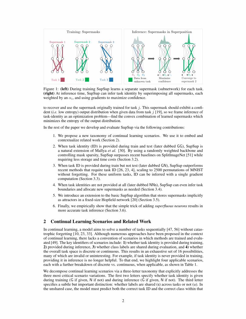
Figure 1: (left) During training SupSup learns a separate supermask (subnetwork) for each task.(right) At inference time, SupSup can infer task identity by superimposing all supermasks, eachweighted by an αi, and using gradients to maximize confidence.

to recover and use the supermask originally trained for task j. This supermask should exhibit a confi-dent (i.e. low entropy) output distribution when given data from task j [19], so we frame inference oftask-identity as an optimization problem—find the convex combination of learned supermasks whichminimizes the entropy of the output distribution.

In the rest of the paper we develop and evaluate SupSup via the following contributions:

1. We propose a new taxonomy of continual learning scenarios. We use it to embed andcontextualize related work (Section 2).

2. When task identity (ID) is provided during train and test (later dubbed GG), SupSup isa natural extension of Mallya et al. [30]. By using a randomly weighted backbone andcontrolling mask sparsity, SupSup surpasses recent baselines on SplitImageNet [51] whilerequiring less storage and time costs (Section 3.2).

3. When task ID is provided during train but not test (later dubbed GN), SupSup outperformsrecent methods that require task ID [26, 23, 4], scaling to 2500 permutations of MNISTwithout forgetting. For these uniform tasks, ID can be inferred with a single gradientcomputation (Section 3.3).

4. When task identities are not provided at all (later dubbed NNs), SupSup can even infer taskboundaries and allocate new supermasks as needed (Section 3.4).

5. We introduce an extension to the basic SupSup algorithm that stores supermasks implicitlyas attractors in a fixed-size Hopfield network [20] (Section 3.5).

6. Finally, we empirically show that the simple trick of adding superfluous neurons results inmore accurate task inference (Section 3.6).

2 Continual Learning Scenarios and Related WorkIn continual learning, a model aims to solve a number of tasks sequentially [47, 56] without catas-trophic forgetting [10, 23, 33]. Although numerous approaches have been proposed in the contextof continual learning, there lacks a convention of scenarios in which methods are trained and evalu-ated [49]. The key identifiers of scenarios include: 1) whether task identity is provided during training,2) provided during inference, 3) whether class labels are shared during evaluation, and 4) whetherthe overall task space is discrete or continuous. This results in an exhaustive set of 16 possibilities,many of which are invalid or uninteresting. For example, if task identity is never provided in training,providing it in inference is no longer helpful. To that end, we highlight four applicable scenarios,each with a further breakdown of discrete vs. continuous, when applicable, as shown in Table 1.

We decompose continual learning scenarios via a three-letter taxonomy that explicitly addresses thethree most critical scenario variations. The first two letters specify whether task identity is givenduring training (G if given, N if not) and during inference (G if given, N if not). The third letterspecifies a subtle but important distinction: whether labels are shared (s) across tasks or not (u). Inthe unshared case, the model must predict both the correct task ID and the correct class within that

2

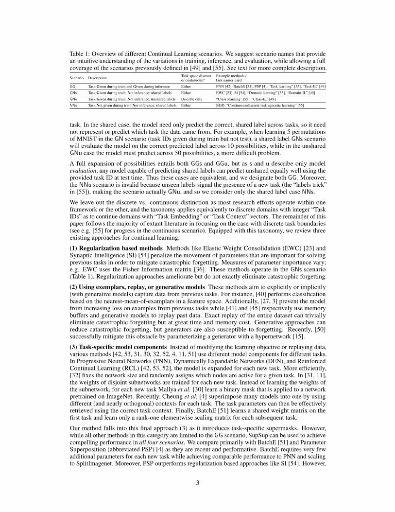
Table 1: Overview of different Continual Learning scenarios. We suggest scenario names that providean intuitive understanding of the variations in training, inference, and evaluation, while allowing a fullcoverage of the scenarios previously defined in [49] and [55]. See text for more complete description.Scenario Description Task space discreet

or continuous?Example methods /task names used

GG Task Given during train and Given during inference Either PNN [42], BatchE [51], PSP [4], “Task learning” [55], “Task-IL” [49]

GNs Task Given during train, Not inference; shared labels Either EWC [23], SI [54], “Domain learning” [55], “Domain-IL” [49]

GNu Task Given during train, Not inference; unshared labels Discrete only “Class learning” [55], “Class-IL” [49]

NNs Task Not given during train Nor inference; shared labels Either BGD, “Continuous/discrete task agnostic learning” [55]

task. In the shared case, the model need only predict the correct, shared label across tasks, so it neednot represent or predict which task the data came from. For example, when learning 5 permutationsof MNIST in the GN scenario (task IDs given during train but not test), a shared label GNs scenariowill evaluate the model on the correct predicted label across 10 possibilities, while in the unsharedGNu case the model must predict across 50 possibilities, a more difficult problem.

A full expansion of possibilities entails both GGs and GGu, but as s and u describe only modelevaluation, any model capable of predicting shared labels can predict unshared equally well using theprovided task ID at test time. Thus these cases are equivalent, and we designate both GG. Moreover,the NNu scenario is invalid because unseen labels signal the presence of a new task (the “labels trick”in [55]), making the scenario actually GNu, and so we consider only the shared label case NNs.

We leave out the discrete vs. continuous distinction as most research efforts operate within oneframework or the other, and the taxonomy applies equivalently to discrete domains with integer “TaskIDs” as to continue domains with “Task Embedding” or “Task Context” vectors. The remainder of thispaper follows the majority of extant literature in focusing on the case with discrete task boundaries(see e.g. [55] for progress in the continuous scenario). Equipped with this taxonomy, we review threeexisting approaches for continual learning.

(1) Regularization based methods Methods like Elastic Weight Consolidation (EWC) [23] andSynaptic Intelligence (SI) [54] penalize the movement of parameters that are important for solvingprevious tasks in order to mitigate catastrophic forgetting. Measures of parameter importance vary;e.g. EWC uses the Fisher Information matrix [36]. These methods operate in the GNs scenario(Table 1). Regularization approaches ameliorate but do not exactly eliminate catastrophic forgetting.

(2) Using exemplars, replay, or generative models These methods aim to explicitly or implicitly(with generative models) capture data from previous tasks. For instance, [40] performs classificationbased on the nearest-mean-of-examplars in a feature space. Additionally, [27, 3] prevent the modelfrom increasing loss on examples from previous tasks while [41] and [45] respectively use memorybuffers and generative models to replay past data. Exact replay of the entire dataset can triviallyeliminate catastrophic forgetting but at great time and memory cost. Generative approaches canreduce catastrophic forgetting, but generators are also susceptible to forgetting. Recently, [50]successfully mitigate this obstacle by parameterizing a generator with a hypernetwork [15].

(3) Task-specific model components Instead of modifying the learning objective or replaying data,various methods [42, 53, 31, 30, 32, 52, 4, 11, 51] use different model components for different tasks.In Progressive Neural Networks (PNN), Dynamically Expandable Networks (DEN), and ReinforcedContinual Learning (RCL) [42, 53, 52], the model is expanded for each new task. More efficiently,[32] fixes the network size and randomly assigns which nodes are active for a given task. In [31, 11],the weights of disjoint subnetworks are trained for each new task. Instead of learning the weights ofthe subnetwork, for each new task Mallya et al. [30] learn a binary mask that is applied to a networkpretrained on ImageNet. Recently, Cheung et al. [4] superimpose many models into one by usingdifferent (and nearly orthogonal) contexts for each task. The task parameters can then be effectivelyretrieved using the correct task context. Finally, BatchE [51] learns a shared weight matrix on thefirst task and learn only a rank-one elementwise scaling matrix for each subsequent task.

Our method falls into this final approach (3) as it introduces task-specific supermasks. However,while all other methods in this category are limited to the GG scenario, SupSup can be used to achievecompelling performance in all four scenarios. We compare primarily with BatchE [51] and ParameterSuperposition (abbreviated PSP) [4] as they are recent and performative. BatchE requires very fewadditional parameters for each new task while achieving comparable performance to PNN and scalingto SplitImagenet. Moreover, PSP outperforms regularization based approaches like SI [54]. However,

3

Algorithm Avg Top 1 BytesAccuracy (%)

Upper Bound 92.55 10222.81M

89.58 195.18MSupSup (GG) 88.68 100.98M

86.37 65.50M

BatchE (GG) 81.50 124.99MSingle Model - 102.23M 106 107 108

Total Number of Bytes

0.5

0.6

0.7

0.8

0.9

Acc

urac

y

Upper Bound

SupSup (GG)

SupSup (GG) Transfer

BatchE (GG)

BatchE (GG) - Rand W

Separate Heads

Separate Heads - Rand W

Figure 2: (left) SplitImagenet performance in Scenario GG. SupSup approaches upper boundperformance with significantly fewer bytes. (right) SplitCIFAR100 performance in Scenario GGshown as mean and standard deviation over 5 seed and splits. SupSup outperforms similar sizebaselines and benefits from transfer.

both BatchE [51] and PSP [4] require task identity to use task-specific weights, so they can onlyoperate in the GG setting.

3 MethodsIn this section, we detail how SupSup leverages supermasks to learn thousands of sequential taskswithout forgetting. We begin with easier settings where task identity is given and gradually move tomore challenging scenarios where task identity is unavailable.

3.1 Preliminaries

In a standard `-way classification task, inputs x are mapped to a distribution p over output neurons{1, ..., `}. We consider the general case where p = f(x,W ) for a neural network f parameterizedby W and trained with a cross-entropy loss. In continual learning classification settings we have kdifferent `-way classification tasks and the input size remains constant across tasks2.

Zhou et al. [57] demonstrate that a trained binary mask (supermask) M can be applied to a randomlyweighted neural network, resulting in a subnetwork with good performance. As further explored byRamanujan et al. [39], supermasks can be trained at similar compute cost to training weights whileachieving performance competitive with weight training.

With supermasks, outputs are given by p = f (x,W �M) where � denotes an elementwise product.W is kept frozen at its initialization: bias terms are 0 and other parameters in W are ±c with equalprobability and c is the standard deviation of the corresponding Kaiming normal distribution [17].This initialization is referred to as signed Kaiming constant by [39] and the constant cmay be differentfor each layer. For completeness we detail the Edge-Popup algorithm for training supermasks [39] inSection E of the appendix.

3.2 Scenario GG: Task Identity Information Given During Train and Inference

When task identity is known during training we can learn a binary mask M i per task. M i are the onlyparameters learned as the weights remain fixed. Given data from task i, outputs are computed as

p = f(x,W �M i

)(1)

For each new task we can either initialize a new supermask randomly, or use a running mean of allsupermasks learned so far. During inference for task i we then use M i. Figure 2 illustrates that inthis scenario SupSup outperforms a number of baselines in accuracy on both SplitCIFAR100 andSplitImageNet while requiring fewer bytes to store. Experiment details are in Section 4.1.

3.3 Scenarios GNs & GNu : Task Identity Information Given During Train Only

We now consider the case where input data comes from task j, but this task information is unknownto the model at inference time. During training we proceed exactly as in Scenario GG, obtaining k

2In practice the tasks do not all need to be `-way — output layers can be padded until all have the same size.

4

learned supermasks. During inference, we aim to infer task identity—correctly detect that the databelongs to task j—and select the corresponding supermask M j .

The SupSup procedure for task ID inference is as follows: first we associate each of the k learnedsupermasks M i with an coefficient αi ∈ [0, 1], initially set to 1/k. Each αi can be interpreted asthe “belief” that supermask M i is the correct mask (equivalently the belief that the current unknowntask is task i). The model’s output is then be computed with a weighted superposition of all learnedmasks:

p(α) = f

(x,W �

(k∑i=1

αiMi

)). (2)

The correct mask M j should produce a confident, low-entropy output [19]. Therefore, to recover thecorrect mask we find the coefficients α which minimize the output entropyH of p(α). One option isto perform gradient descent on α via

α← α− η∇αH (p (α)) (3)

where η is the step size, and αs are re-normalized to sum to one after each update. Another option isto try each mask individually and pick the one with the lowest entropy output requiring k forwardpasses. However, we want an optimization method with fixed sub-linear run time (w.r.t. the numberof tasks k) which leads α to a corner of the probability simplex — i.e. α is 0 everywhere except fora single 1. We can then take the nonzero index to be the inferred task. To this end we consider theOne-Shot and Binary algorithms.

One-Shot: The task is inferred using a single gradient. Specifically, the inferred task is given by

arg maxi

(−∂H (p (α))

∂αi

)(4)

as entropy is decreasing maximally in this coordinate. This algorithms corresponds to one step of theFrank-Wolfe algorithm [7], or one-step of gradient descent followed by softmax re-normalizationwith the step size η approaching∞. Unless noted otherwise, x is a single image and not a batch.

Binary: Resembling binary search, we infer task identity using an algorithm with log k steps.At each step we rule out half the tasks—the tasks corresponding to entries in the bottom half of−∇αH (p (α)). These are the coordinates in which entropy is minimally decreasing. A task i isruled out by setting αi to zero and at each step we re-normalize the remaining entries in α so thatthey sum to one. Pseudo-code for both algorithms may be found in Section A of the appendix.

Once the task is inferred the corresponding mask can be used as in Equation 1 to obtain classprobabilities p. In both Scenario GNs and GNu the class probabilities p are returned. In GNu,p forms a distribution over the classes corresponding to the inferred task. Experiments solvingthousands of tasks are detailed in Section 4.2.

3.4 Scenario NNs: No Task Identity During Training or Inference

Task inference algorithms from Scenario GN enable the extension of SupSup to Scenario NNs, wheretask identity is entirely unknown (even during training). If SupSup is uncertain about the currenttask identity, it is likely that the data do not belong to any task seen so far. When this occurs a newsupermask is allocated, and k (the number of tasks learned so far) is incremented.

We consider the One-Shot algorithm and say that SupSup is uncertain when performing task identityinference if ν = softmax (−∇αH (p (α))) is approximately uniform. Specifically, if kmaxi νi <1 + ε a new mask is allocated and k is incremented. Otherwise mask arg maxi νi is used, whichcorresponds to Equation 4. We conduct experiments on learning up to 2500 tasks entirely withoutany task information, detailed in Section 4.3. Figure 4 shows that SupSup in Scenario NNs achievescomparable performance even to Scenario GNu.

3.5 Beyond Linear Memory Dependence

Hopfield networks [20] implicitly encode a series of binary strings zi ∈ {−1, 1}d with an associatedenergy function EΨ(z) =

∑uv Ψuvzuzv. Each zi is a minima of EΨ, and can be recovered with

gradient descent. Ψ ∈ Rd×d is initially 0, and to encode a new string zi, Ψ← Ψ + 1dzizi>.

5

10 50 100 150 200 250Num Tasks Learned

0.88

0.90

0.92

0.94

0.96

0.98

Acc

urac

y


SupSup (GNu, H) SupSup (GNu, G) PSP (GG) BatchE (GG) Upper Bound

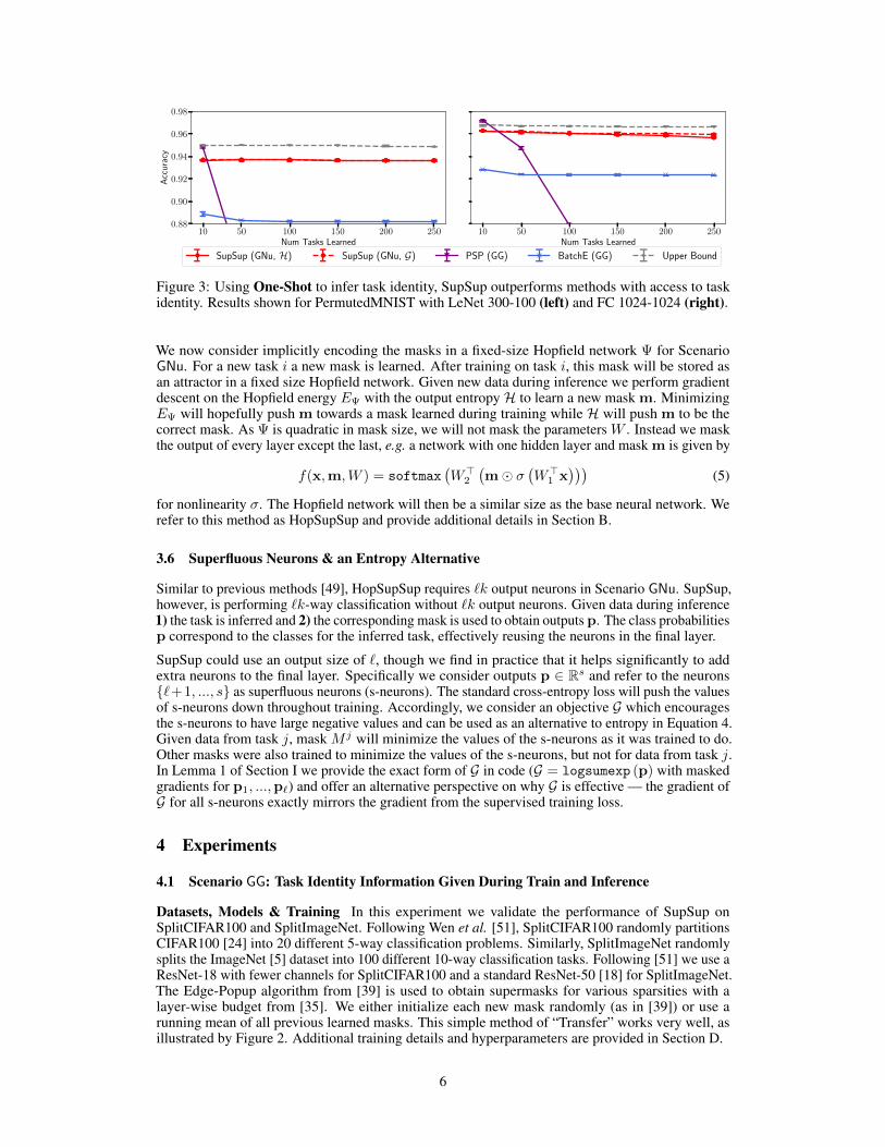
Figure 3: Using One-Shot to infer task identity, SupSup outperforms methods with access to taskidentity. Results shown for PermutedMNIST with LeNet 300-100 (left) and FC 1024-1024 (right).

We now consider implicitly encoding the masks in a fixed-size Hopfield network Ψ for ScenarioGNu. For a new task i a new mask is learned. After training on task i, this mask will be stored asan attractor in a fixed size Hopfield network. Given new data during inference we perform gradientdescent on the Hopfield energy EΨ with the output entropyH to learn a new mask m. MinimizingEΨ will hopefully push m towards a mask learned during training while H will push m to be thecorrect mask. As Ψ is quadratic in mask size, we will not mask the parameters W . Instead we maskthe output of every layer except the last, e.g. a network with one hidden layer and mask m is given by

f(x,m,W ) = softmax(W>2

(m� σ

(W>1 x

)))(5)

for nonlinearity σ. The Hopfield network will then be a similar size as the base neural network. Werefer to this method as HopSupSup and provide additional details in Section B.

3.6 Superfluous Neurons & an Entropy Alternative

Similar to previous methods [49], HopSupSup requires `k output neurons in Scenario GNu. SupSup,however, is performing `k-way classification without `k output neurons. Given data during inference1) the task is inferred and 2) the corresponding mask is used to obtain outputs p. The class probabilitiesp correspond to the classes for the inferred task, effectively reusing the neurons in the final layer.

SupSup could use an output size of `, though we find in practice that it helps significantly to addextra neurons to the final layer. Specifically we consider outputs p ∈ Rs and refer to the neurons{`+1, ..., s} as superfluous neurons (s-neurons). The standard cross-entropy loss will push the valuesof s-neurons down throughout training. Accordingly, we consider an objective G which encouragesthe s-neurons to have large negative values and can be used as an alternative to entropy in Equation 4.Given data from task j, mask M j will minimize the values of the s-neurons as it was trained to do.Other masks were also trained to minimize the values of the s-neurons, but not for data from task j.In Lemma 1 of Section I we provide the exact form of G in code (G = logsumexp (p) with maskedgradients for p1, ...,p`) and offer an alternative perspective on why G is effective — the gradient ofG for all s-neurons exactly mirrors the gradient from the supervised training loss.

4 Experiments

4.1 Scenario GG: Task Identity Information Given During Train and Inference

Datasets, Models & Training In this experiment we validate the performance of SupSup onSplitCIFAR100 and SplitImageNet. Following Wen et al. [51], SplitCIFAR100 randomly partitionsCIFAR100 [24] into 20 different 5-way classification problems. Similarly, SplitImageNet randomlysplits the ImageNet [5] dataset into 100 different 10-way classification tasks. Following [51] we use aResNet-18 with fewer channels for SplitCIFAR100 and a standard ResNet-50 [18] for SplitImageNet.The Edge-Popup algorithm from [39] is used to obtain supermasks for various sparsities with alayer-wise budget from [35]. We either initialize each new mask randomly (as in [39]) or use arunning mean of all previous learned masks. This simple method of “Transfer” works very well, asillustrated by Figure 2. Additional training details and hyperparameters are provided in Section D.

6

0 1000 2000Num Tasks Learned

0.91

0.92

0.93

0.94

0.95

Acc

urac

y

Upper Bound SupSup (GNu, H) SupSup (GNu, G) Lower Bound SupSup (NNs, H)


0.4

0.6

0.8

Acc

urac

y

Upper Bound SupSup (GNu, H) SupSup (GNu, G) Lower Bound SupSup (NNs, H)


0.4

0.6

0.8

Acc

urac

y

SupSup (NNs, H) SupSup (GNu, H) SupSup (GNu, G) Upper Bound Lower Bound

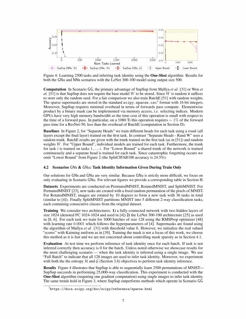
Figure 4: Learning 2500 tasks and inferring task identity using the One-Shot algorithm. Results forboth the GNu and NNs scenarios with the LeNet 300-100 model using output size 500.

Computation In Scenario GG, the primary advantage of SupSup from Mallya et al. [31] or Wen etal. [51] is that SupSup does not require the base model W to be stored. Since W is random it sufficesto store only the random seed. For a fair comparison we also train BatchE [51] with random weights.The sparse supermasks are stored in the standard scipy.sparse.csc3 format with 16 bit integers.Moreover, SupSup requires minimal overhead in terms of forwards pass compute. Elementwiseproduct by a binary mask can be implemented via memory access, i.e. selecting indices. ModernGPUs have very high memory bandwidth so the time cost of this operation is small with respect tothe time of a forward pass. In particular, on a 1080 Ti this operation requires ∼ 1% of the forwardpass time for a ResNet-50, less than the overhead of BatchE (computation in Section D).

Baselines In Figure 2, for “Separate Heads” we train different heads for each task using a trunk (alllayers except the final layer) trained on the first task. In contrast “Separate Heads - Rand W” uses arandom trunk. BatchE results are given with the trunk trained on the first task (as in [51]) and randomweights W . For “Upper Bound”, individual models are trained for each task. Furthermore, the trunkfor task i is trained on tasks 1, ..., i. For “Lower Bound” a shared trunk of the network is trainedcontinuously and a separate head is trained for each task. Since catastrophic forgetting occurs weomit “Lower Bound” from Figure 2 (the SplitCIFAR100 accuracy is 24.5%).

4.2 Scenarios GNs & GNu: Task Identity Information Given During Train Only

Our solutions for GNs and GNu are very similar. Because GNu is strictly more difficult, we focus ononly evaluating in Scenario GNu. For relevant figures we provide a corresponding table in Section H.

Datasets Experiments are conducted on PermutedMNIST, RotatedMNIST, and SplitMNIST. ForPermutedMNIST [23], new tasks are created with a fixed random permutation of the pixels of MNIST.For RotatedMNIST, images are rotated by 10 degrees to form a new task with 36 tasks in total(similar to [4]). Finally SplitMNIST partitions MNIST into 5 different 2-way classification tasks,each containing consecutive classes from the original dataset.

Training We consider two architectures: 1) a fully connected network with two hidden layers ofsize 1024 (denoted FC 1024-1024 and used in [4]) 2) the LeNet 300-100 architecture [25] as usedin [8, 6]. For each task we train for 1000 batches of size 128 using the RMSProp optimizer [48]with learning rate 0.0001 which follows the hyperparameters of [4]. Supermasks are found usingthe algorithm of Mallya et al. [31] with threshold value 0. However, we initialize the real valued“scores” with Kaiming uniform as in [39]. Training the mask is not a focus of this work, we choosethis method as it is fast and we are not concerned about controlling mask sparsity as in Section 4.1.

Evaluation At test time we perform inference of task identity once for each batch. If task is notinferred correctly then accuracy is 0 for the batch. Unless noted otherwise we showcase results forthe most challenging scenario — when the task identity is inferred using a single image. We use“Full Batch” to indicate that all 128 images are used to infer task identity. Moreover, we experimentwith both the the entropyH and G (Section 3.6) objectives to perform task identity inference.

Results Figure 4 illustrates that SupSup is able to sequentially learn 2500 permutations of MNIST—SupSup succeeds in performing 25,000-way classification. This experiment is conducted with theOne-Shot algorithm (requiring one gradient computation) using single images to infer task identity.The same trends hold in Figure 3, where SupSup outperforms methods which operate in Scenario GG

3https://docs.scipy.org/doc/scipy/reference/sparse.html

7

https://docs.scipy.org/doc/scipy/reference/sparse.html

0 50 100 150 200 250 300 350Rotation (degrees)

0.90

0.95

1.00

Acc

urac

y

SupSup (GNu, full batch, H)

BatchE (GG)

PSP (GG)

Upper Bound

Lower Bound


0.5

0.6

0.7

0.8

0.9

1.0

Acc

urac

y

SupSup (GNu, H)

BatchE (GNu, full batch, H)

BatchE (GNu, H)

Upper Bound

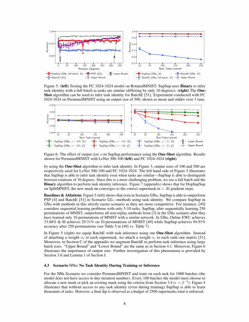
Figure 5: (left) Testing the FC 1024-1024 model on RotatedMNIST. SupSup uses Binary to infertask identity with a full batch as tasks are similar (differing by only 10 degrees). (right) The One-Shot algorithm can be used to infer task identity for BatchE [51]. Experiment conducted with FC1024-1024 on PermutedMNIST using an output size of 500, shown as mean and stddev over 3 runs.


0.90

0.92

0.94

0.96

0.98

Acc

urac

y


SupSup (GNu, s = 200, H)

SupSup (GNu, s = 200, G)





Lower Bound

Upper Bound

Figure 6: The effect of output size s on SupSup performance using the One-Shot algorithm. Resultsshown for PermutedMNIST with LeNet 300-100 (left) and FC 1024-1024 (right).

by using the One-Shot algorithm to infer task identity. In Figure 3, output sizes of 100 and 500 arerespectively used for LeNet 300-100 and FC 1024-1024. The left hand side of Figure 5 illustratesthat SupSup is able to infer task identity even when tasks are similar—SupSup is able to distinguishbetween rotations of 10 degrees. Since this is a more challenging problem, we use a full batch and theBinary algorithm to perform task identity inference. Figure 7 (appendix) shows that for HopSupSupon SplitMNIST, the new mask m converges to the correct supermask in < 30 gradient steps.

Baselines & Ablations Figure 5 (left) shows that even in Scenario GNu, SupSup is able to outperformPSP [4] and BatchE [51] in Scenario GG—methods using task identity. We compare SupSup inGNu with methods in this strictly easier scenario as they are more competitive. For instance, [49]considers sequential learning problems with only 5-10 tasks. SupSup, after sequentially learning 250permutations of MNIST, outperforms all non-replay methods from [3] in the GNu scenario after theyhave learned only 10 permutations of MNIST with a similar network. In GNu, Online EWC achieves33.88% & SI achieves 29.31% on 10 permutations of MNIST [49] while SupSup achieves 94.91%accuracy after 250 permutations (see Table 5 in [49] vs. Table 7).

In Figure 5 (right) we equip BatchE with task inference using our One-Shot algorithm. Insteadof attaching a weight αi to each supermask, we attach a weight αi to each rank-one matrix [51].Moreover, in Section C of the appendix we augment BatchE to perform task-inference using largebatch sizes. “Upper Bound” and “Lower Bound” are the same as in Section 4.1. Moreover, Figure 6illustrates the importance of output size. Further investigation of this phenomena is provided bySection 3.6 and Lemma 1 of Section I.

4.3 Scenario NNs: No Task Identity During Training or Inference

For the NNs Scenario we consider PermutedMNIST and train on each task for 1000 batches (themodel does not have access to this iteration number). Every 100 batches the model must choose toallocate a new mask or pick an existing mask using the criteria from Section 3.4 (ε = 2−3). Figure 4illustrates that without access to any task identity (even during training) SupSup is able to learnthousands of tasks. However, a final dip is observed as a budget of 2500 supermasks total is enforced.

8

5 Conclusion

Supermasks in Superposition (SupSup) is a flexible and compelling model applicable to a widerange of scenarios in Continual Learning. SupSup leverages the power of subnetworks [57, 39, 31],and gradient-based optimization to infer task identity when unknown. SupSup achieves state-of-the-art performance on SplitImageNet when given task identity, and performs well on thousands ofpermutations and almost indiscernible rotations of MNIST without any task information.

We observe limitations in applying SupSup with task identity inference to non-uniform and morechallenging problems. Task inference fails when models are not well calibrated—are overly confidentfor the wrong task. As future work, we hope to explore automatic task inference with more calibratedmodels [14], as well as circumventing calibration challenges by using optimization objectives suchas self-supervision [16] and energy based models [13]. In doing so, we hope to tackle large-scaleproblems in Scenarios GN and NNs.

Broader Impact

A goal of continual learning is to solve many tasks with a single model. However, it is not exactlyclear what qualifies as a single model. Therefore, a concrete objective has become to learn manytasks as efficiently as possible. We believe that SupSup is a useful step in this direction. However,there are consequences to more efficient models, both positive and negative.

We begin with the positive consequences:

• Efficient models require less compute, and are therefore less harmful for the environmentthen learning one model per task [44]. This is especially true if models are able to leverageinformation from past tasks, and training on new tasks is then faster.

• Efficient models may be run on the end device. This helps to preserve privacy as a user’sdata does not have to be sent to the cloud for computation.

• If models are more efficient then large scale research is not limited to wealthier institutions.These institutions are more likely in privileged parts of the world and may be ignorantof problems facing developing nations. Moreover, privileged institutions may not be arepresentative sample of the research community.

We would also like to highlight and discuss the negative consequences of models which can efficientlylearn many tasks, and efficient models in general. When models are more efficient, they are also moreavailable and less subject to regularization and study as a result. For instance, when a high-impactmodel is released by an institution it will hopefully be accompanied by a Model Card [34] analyzingthe bias and intended use of the model. By contrast, if anyone is able to train a powerful model thismay no longer be the case, resulting in a proliferation of models with harmful biases or intended use.Taking the United States for instance, bias can be harmful as models show disproportionately moreerrors for already marginalized groups [2], furthering existing and deeply rooted structural racism.

Acknowledgments

We thank Gabriel Ilharco Magalhães and Sarah Pratt for helpful comments. For valuable conversationswe also thank Tim Dettmers, Kiana Ehsani, Ana Marasovic, Suchin Gururangan, Zoe Steine-Hanson,Connor Shorten, Samir Yitzhak Gadre, Samuel McKinney and Kishanee Haththotuwegama. Thiswork is in part supported by NSF IIS 1652052, IIS 17303166, DARPA N66001-19-2-4031, DARPAW911NF-15-1-0543 and gifts from Allen Institute for Artificial Intelligence. Additional revenues:co-authors had employment with the Allen Institute for AI.

References

[1] Yoshua Bengio, Nicolas L Roux, Pascal Vincent, Olivier Delalleau, and Patrice Marcotte.Convex neural networks. In Advances in neural information processing systems, pages 123–130,2006.

9

[2] Joy Buolamwini and Timnit Gebru. Gender shades: Intersectional accuracy disparities incommercial gender classification. In Conference on fairness, accountability and transparency,pages 77–91, 2018.

[3] Arslan Chaudhry, Marc’Aurelio Ranzato, Marcus Rohrbach, and Mohamed Elhoseiny. Efficientlifelong learning with a-gem. arXiv preprint arXiv:1812.00420, 2018.

[4] Brian Cheung, Alexander Terekhov, Yubei Chen, Pulkit Agrawal, and Bruno Olshausen. Su-perposition of many models into one. In Advances in Neural Information Processing Systems,pages 10867–10876, 2019.

[5] Jia Deng, Wei Dong, Richard Socher, Li-Jia Li, Kai Li, and Li Fei-Fei. Imagenet: A large-scalehierarchical image database. In CVPR 2009, 2009.

[6] Tim Dettmers and Luke Zettlemoyer. Sparse networks from scratch: Faster training withoutlosing performance. arXiv preprint arXiv:1907.04840, 2019.

[7] Marguerite Frank and Philip Wolfe. An algorithm for quadratic programming. Naval researchlogistics quarterly, 3(1-2):95–110, 1956.

[8] Jonathan Frankle and Michael Carbin. The lottery ticket hypothesis: Finding sparse, trainableneural networks. arXiv preprint arXiv:1803.03635, 2018.

[9] Jonathan Frankle, David J Schwab, and Ari S Morcos. Training batchnorm and only batchnorm:On the expressive power of random features in cnns. arXiv preprint arXiv:2003.00152, 2020.

[10] Robert M French. Catastrophic forgetting in connectionist networks. Trends in cognitivesciences, 3(4):128–135, 1999.

[11] Siavash Golkar, Michael Kagan, and Kyunghyun Cho. Continual learning via neural pruning.arXiv preprint arXiv:1903.04476, 2019.

[12] Ian J Goodfellow, Mehdi Mirza, Da Xiao, Aaron Courville, and Yoshua Bengio. An empiricalinvestigation of catastrophic forgetting in gradient-based neural networks. arXiv preprintarXiv:1312.6211, 2013.

[13] Will Grathwohl, Kuan-Chieh Wang, Jörn-Henrik Jacobsen, David Duvenaud, MohammadNorouzi, and Kevin Swersky. Your classifier is secretly an energy based model and you shouldtreat it like one. arXiv preprint arXiv:1912.03263, 2019.

[14] Chuan Guo, Geoff Pleiss, Yu Sun, and Kilian Q Weinberger. On calibration of modern neuralnetworks. In Proceedings of the 34th International Conference on Machine Learning-Volume70, pages 1321–1330. JMLR. org, 2017.

[15] David Ha, Andrew Dai, and Quoc V Le. Hypernetworks. arXiv preprint arXiv:1609.09106,2016.

[16] Kaiming He, Haoqi Fan, Yuxin Wu, Saining Xie, and Ross Girshick. Momentum contrast forunsupervised visual representation learning. arXiv preprint arXiv:1911.05722, 2019.

[17] Kaiming He, Xiangyu Zhang, Shaoqing Ren, and Jian Sun. Delving deep into rectifiers:Surpassing human-level performance on imagenet classification. In Proceedings of the IEEEinternational conference on computer vision, pages 1026–1034, 2015.

[18] Kaiming He, Xiangyu Zhang, Shaoqing Ren, and Jian Sun. Deep residual learning for imagerecognition. In Proceedings of the IEEE conference on computer vision and pattern recognition,pages 770–778, 2016.

[19] Dan Hendrycks and Kevin Gimpel. A baseline for detecting misclassified and out-of-distributionexamples in neural networks. arXiv preprint arXiv:1610.02136, 2016.

[20] John J Hopfield. Neural networks and physical systems with emergent collective computationalabilities. Proceedings of the national academy of sciences, 79(8):2554–2558, 1982.

[21] Sergey Ioffe and Christian Szegedy. Batch normalization: Accelerating deep network trainingby reducing internal covariate shift. arXiv preprint arXiv:1502.03167, 2015.

[22] Diederik P Kingma and Jimmy Ba. Adam: A method for stochastic optimization. arXiv preprintarXiv:1412.6980, 2014.

[23] James Kirkpatrick, Razvan Pascanu, Neil Rabinowitz, Joel Veness, Guillaume Desjardins,Andrei A Rusu, Kieran Milan, John Quan, Tiago Ramalho, Agnieszka Grabska-Barwinska, et al.Overcoming catastrophic forgetting in neural networks. Proceedings of the national academy ofsciences, 114(13):3521–3526, 2017.

10

[24] Alex Krizhevsky. Learning multiple layers of features from tiny images. Technical report,University of Toronto, 2009.

[25] Yann LeCun, Bernhard Boser, John S Denker, Donnie Henderson, Richard E Howard, WayneHubbard, and Lawrence D Jackel. Backpropagation applied to handwritten zip code recognition.Neural computation, 1(4):541–551, 1989.

[26] Yann LeCun, Corinna Cortes, and CJ Burges. Mnist handwritten digit database. 2010.[27] David Lopez-Paz and Marc’Aurelio Ranzato. Gradient episodic memory for continual learning.

In Advances in Neural Information Processing Systems, pages 6467–6476, 2017.[28] Ilya Loshchilov and Frank Hutter. Sgdr: Stochastic gradient descent with warm restarts, 2016.[29] Eran Malach, Gilad Yehudai, Shai Shalev-Shwartz, and Ohad Shamir. Proving the lottery ticket

hypothesis: Pruning is all you need. arXiv preprint arXiv:2002.00585, 2020.[30] Arun Mallya, Dillon Davis, and Svetlana Lazebnik. Piggyback: Adapting a single network to

multiple tasks by learning to mask weights. In Proceedings of the European Conference onComputer Vision (ECCV), pages 67–82, 2018.

[31] Arun Mallya and Svetlana Lazebnik. Packnet: Adding multiple tasks to a single network byiterative pruning. In Proceedings of the IEEE Conference on Computer Vision and PatternRecognition, pages 7765–7773, 2018.

[32] Nicolas Y Masse, Gregory D Grant, and David J Freedman. Alleviating catastrophic forgettingusing context-dependent gating and synaptic stabilization. Proceedings of the National Academyof Sciences, 115(44):E10467–E10475, 2018.

[33] Michael McCloskey and Neal J Cohen. Catastrophic interference in connectionist networks:The sequential learning problem. In Psychology of learning and motivation, volume 24, pages109–165. Elsevier, 1989.

[34] Margaret Mitchell, Simone Wu, Andrew Zaldivar, Parker Barnes, Lucy Vasserman, Ben Hutchin-son, Elena Spitzer, Inioluwa Deborah Raji, and Timnit Gebru. Model cards for model reporting.In Proceedings of the conference on fairness, accountability, and transparency, pages 220–229,2019.

[35] Decebal Constantin Mocanu, Elena Mocanu, Peter Stone, Phuong H Nguyen, MadeleineGibescu, and Antonio Liotta. Scalable training of artificial neural networks with adaptive sparseconnectivity inspired by network science. Nature communications, 9(1):1–12, 2018.

[36] Razvan Pascanu and Yoshua Bengio. Revisiting natural gradient for deep networks. arXivpreprint arXiv:1301.3584, 2013.

[37] Adam Paszke, Sam Gross, Francisco Massa, Adam Lerer, James Bradbury, Gregory Chanan,Trevor Killeen, Zeming Lin, Natalia Gimelshein, Luca Antiga, et al. Pytorch: An imperativestyle, high-performance deep learning library. In Advances in Neural Information ProcessingSystems, pages 8024–8035, 2019.

[38] Prajit Ramachandran, Barret Zoph, and Quoc V Le. Searching for activation functions. arXivpreprint arXiv:1710.05941, 2017.

[39] Vivek Ramanujan, Mitchell Wortsman, Aniruddha Kembhavi, Ali Farhadi, and Moham-mad Rastegari. What’s hidden in a randomly weighted neural network? arXiv preprintarXiv:1911.13299, 2019.

[40] Sylvestre-Alvise Rebuffi, Alexander Kolesnikov, Georg Sperl, and Christoph H Lampert. icarl:Incremental classifier and representation learning. In Proceedings of the IEEE conference onComputer Vision and Pattern Recognition, pages 2001–2010, 2017.

[41] David Rolnick, Arun Ahuja, Jonathan Schwarz, Timothy Lillicrap, and Gregory Wayne. Expe-rience replay for continual learning. In Advances in Neural Information Processing Systems,pages 348–358, 2019.

[42] Andrei A Rusu, Neil C Rabinowitz, Guillaume Desjardins, Hubert Soyer, James Kirkpatrick,Koray Kavukcuoglu, Razvan Pascanu, and Raia Hadsell. Progressive neural networks. arXivpreprint arXiv:1606.04671, 2016.

[43] Benjamin Schrauwen, David Verstraeten, and Jan Van Campenhout. An overview of reservoircomputing: theory, applications and implementations. In Proceedings of the 15th europeansymposium on artificial neural networks. p. 471-482 2007, pages 471–482, 2007.

11

[44] Roy Schwartz, Jesse Dodge, Noah A Smith, and Oren Etzioni. Green ai. corr abs/1907.10597(2019). arXiv preprint arXiv:1907.10597, 2019.

[45] Hanul Shin, Jung Kwon Lee, Jaehong Kim, and Jiwon Kim. Continual learning with deepgenerative replay. In Advances in Neural Information Processing Systems, pages 2990–2999,2017.

[46] Amos Storkey. Increasing the capacity of a hopfield network without sacrificing functionality.In International Conference on Artificial Neural Networks, pages 451–456. Springer, 1997.

[47] Sebastian Thrun. Lifelong learning algorithms. In Learning to learn, pages 181–209. Springer,1998.

[48] Tijmen Tieleman and Geoffrey Hinton. Lecture 6.5-rmsprop: Divide the gradient by a runningaverage of its recent magnitude. COURSERA: Neural networks for machine learning, 4(2):26–31, 2012.

[49] Gido M van de Ven and Andreas S Tolias. Three scenarios for continual learning. arXiv preprintarXiv:1904.07734, 2019.

[50] Johannes von Oswald, Christian Henning, João Sacramento, and Benjamin F. Grewe. Continuallearning with hypernetworks. In International Conference on Learning Representations, 2020.

[51] Yeming Wen, Dustin Tran, and Jimmy Ba. Batchensemble: an alternative approach to efficientensemble and lifelong learning. arXiv preprint arXiv:2002.06715, 2020.

[52] Ju Xu and Zhanxing Zhu. Reinforced continual learning. In Advances in Neural InformationProcessing Systems, pages 899–908, 2018.

[53] Jaehong Yoon, Eunho Yang, Jeongtae Lee, and Sung Ju Hwang. Lifelong learning withdynamically expandable networks. arXiv preprint arXiv:1708.01547, 2017.

[54] Friedemann Zenke, Ben Poole, and Surya Ganguli. Continual learning through synapticintelligence. In Proceedings of the 34th International Conference on Machine Learning-Volume70, pages 3987–3995. JMLR. org, 2017.

[55] Chen Zeno, Itay Golan, Elad Hoffer, and Daniel Soudry. Task agnostic continual learning usingonline variational bayes. arXiv preprint arXiv:1803.10123, 2018.

[56] Jieyu Zhao and Jurgen Schmidhuber. Incremental self-improvement for life-time multi-agentreinforcement learning. In From Animals to Animats 4: Proceedings of the Fourth InternationalConference on Simulation of Adaptive Behavior, Cambridge, MA, pages 516–525, 1996.

[57] Hattie Zhou, Janice Lan, Rosanne Liu, and Jason Yosinski. Deconstructing lottery tickets:Zeros, signs, and the supermask. In Advances in Neural Information Processing Systems, pages3592–3602, 2019.

12