International Journal of Heat and Fluid Flow 32 (2011) 1057–1067

Contents lists available at ScienceDirect

International Journal of Heat and Fluid Flow

journal homepage: www.elsevier .com/ locate/ i jhf f

Three-dimensional CFD simulation of bubble–melt two-phase flow withair injecting and melt stirring

Hong Liu a,⇑, Maozhao Xie a, Ke Li a, Deqing Wang b

a School of Energy and Power Engineering, Dalian University of Technology, Dalian 116024, Chinab College of Material Science and Engineering, Dalian Jiaotong University, Dalian 116024, China

a r t i c l e i n f o a b s t r a c t

Article history:Received 18 August 2010Received in revised form 8 June 2011Accepted 9 June 2011Available online 7 July 2011

Keywords:BubbleMetallic meltNumber density functionBreak-upCoalescence

0142-727X/$ - see front matter � 2011 Elsevier Inc. Adoi:10.1016/j.ijheatfluidflow.2011.06.003

⇑ Corresponding author. Tel.: +86 411 84706302; faE-mail address: hongliu@dlut.edu.cn (H. Liu).

This paper reports on progress in developing CFD simulations of gas bubble–metallic melt turbulent flowsinduced by a pitched-blade impeller with an inclined shaft. Foaming process of aluminum foams, inwhich air is injected into molten aluminum composites and the melt is mechanical stirred by the impel-ler, has been investigated. A two-fluid model, incorporated with the Multiple Reference Frames (MRF)method is used to predict the three-dimensional gas–liquid flow in the foaming tank, in which a stirringshaft is positioned inclined into the melt. Locally average bubble size is also predicted by additively solv-ing a transport equation for the bubble number density function, which accounts for effects of bubblebreakup and coalescence phenomena. The computed bubble sizes are compared with experimental datafrom our water model measurement and reasonable agreements are obtained. Further, simulated resultsshow that the volume averaged total and local gas fractions are generally increased with rising impellerspeed and gas flow rate. The local averaged bubble size increases with increasing gas flow rate and orificediameter and decreasing liquid viscosity, and decreases also with rising rotation speed of the impeller.

� 2011 Elsevier Inc. All rights reserved.

1. Introduction

Aluminum foams, as a representative of metallic foams, are akind of very useful and promising functional materials. Theadvancement in the techniques for production of aluminum foamshas expanded their use over a wide range of applications, includinglightweight structural sandwich panels in Schwingel et al. (2007),and Zhao et al. (2008), and energy absorption devices in Chenget al. (2006). There are various approaches to produce aluminumfoams, such as foaming of melts with blowing agents, foaming ofmelts by gas injection, foaming of metal powder compacts and soon, from which the gas injection method has outstanding advanta-ges in the respect that metallic foams can be produced continu-ously and the size of the product is little limited. In thistechnique, air is injected through few nozzles into molten alumi-num composites. The air injecting and the impeller stirring causebubbles rise to the top surface of the melt, forming a liquid foambody, which is stabilized by the presence of solid ceramic particlesat gas–liquid interfaces of the cell walls. The stabilized liquid foamis then mechanically conveyed off the surface of the melt and al-lowed to cool to form a solid slab of aluminum foam.

ll rights reserved.

x: +86 411 84708460.

Both physical and mechanical properties of aluminum foamsare not only controlled by their composition, they are also affectedsignificantly by cell structure (Riveiro et al., 2007; Styles et al.,2007). The cell structure (cell size and cell wall thickness) is con-trolled by the processing variables such as the size and volumefraction of the solid particles, foaming temperature, air flow rate,impeller design and impeller rotation speed during the foam mak-ing process. Unfortunately, no open publication has been foundworking on the influence of processing variables on the foam cellstructure of aluminum foams. This might be due to the difficultiesin experimental observation and measurement because of the non-transparency and high temperature of the metallic melt. On theother hand, numerical simulation has become a very importantand powerful tool for investigating and understanding complexflow phenomena in science and engineering. Over recent yearsmore and more efforts have been made to investigate metal meltflows, both one-phase and two-phases, by numerical simulations(Johansen, 2002; Lane et al., 2002; Mazumdar and Evans, 2004;Xia et al., 2001; Liu and Schwarz, 2009).

However, fluid dynamics in a bubble–melt two-phase system ishighly complex, especially when it is coupled with gas injectionand is stirred by an inclined impeller. To the authors’ knowledgeso far there is no open literature reporting on numerical modelingof such flow processes. Related studies can be found mainly in twoareas. One is the flow in a stirred tank. A great number of investi-gations on gas–liquid turbulent two-phase flow in stirred tanks

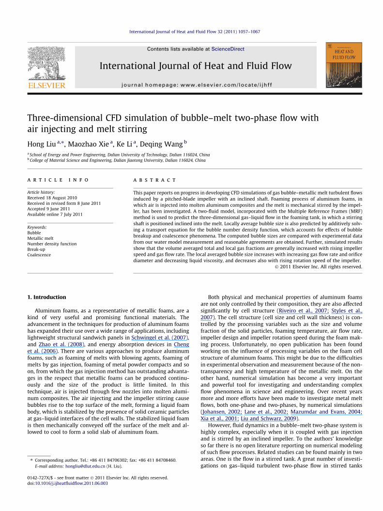
(a) Experimental setup for foaming (b) Propeller design. experiments.

Fig. 1. Schematic diagram of experimental apparatus.

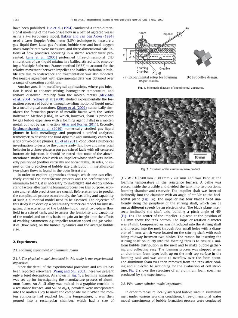
Fig. 2. Structure of the aluminum foam product.

1058 H. Liu et al. / International Journal of Heat and Fluid Flow 32 (2011) 1057–1067

have been published. Luo et al. (1994) conducted a three-dimen-sional modeling of the two-phase flow in a baffled agitated vesselusing a k–e turbulence model. Bakker and van den Akker (1994)used a Laser Doppler Velocimeter (LDV) technique to measure agas–liquid flow. Local gas fraction, bubble size and local oxygenmass transfer rate were measured, and three-dimensional calcula-tions of flow processes occurring in a stirred reactor were pre-sented. Lane et al. (2005) performed three-dimensional CFDsimulations of gas–liquid mixing in a baffled stirred tank, employ-ing a Multiple Reference Frames method (MRF) to account for therelative movement between impeller and baffles. Variation in bub-ble size due to coalescence and fragmentation was also modeled.Reasonable agreement with experimental data was obtained overa range of operating conditions.

Another area is in metallurgical applications, where gas injec-tion is used to enhance mixing, homogenize temperature, andremove dissolved impurity from the molten metals (Alexiadiset al., 2004). Yokoya et al. (2000) studied experimentally the for-mation process of bubbles through swirling motion of liquid metalin a metallurgical container. Körner et al. (2002) numerically sim-ulated the formation process of metallic foams with the LatticeBoltzmann Method (LBM), in which, however, foam is producedby gas bubble expansion with a foaming agent (TiH2) in a moltenmetal, but not by gas injection (Attar and Korner, 2011). Recently,Krishnapisharody et al. (2010) numerically studied gas–liquidplumes in ladle metallurgy, and proposed a unified analyticalframework to describe the fluid dynamic and similarity character-istics of two-phase plumes. Liu et al. (2011) conducted a numericalinvestigation to describe the quasi-steady fluid flow and interfacialbehavior in a three-phase argon gas-stirred ladle with off-centeredbottom air injection. It should be noted that none of the above-mentioned studies dealt with an impeller whose shaft was inclin-edly positioned (neither vertically nor horizontally). Besides, no re-port on the prediction of bubble size distribution in metallurgicaltwo-phase flows is found in the open literature.

In order to explore approaches through which one can effec-tively control the manufacture process and the performances ofaluminum foams, it is necessary to investigate and deeply under-stand factors affecting the foaming process. For this purpose, accu-rate and reliable predictions are crucial. Before attempts to predictthe complicated processes accurately, the feasibility and capabilityof such a numerical model need to be assessed. The objective ofthis study is to develop a preliminary numerical model for investi-gating characteristics of the bubble–liquid metal two-phase flowfield in a stirred tank, and to assess the feasibility and capabilityof the model, and on this basis, to gain an insight into the effectsof working parameters, e.g. impeller rotation speed and gas veloc-ities (flow rate), on the bubble dynamics and the average bubblesize.

2. Experiments

2.1. Foaming experiment of aluminum foams

2.1.1. The physical model simulated in this study is our experimentalapparatus

Since the detail of the experimental procedure and results hasbeen reported elsewhere (Wang and Shi, 2003), here we presentonly a brief description. As shown in Fig. 1, a foaming apparatuswas set up for investigating the manufacture process of alumi-num foams. An Al–Si alloy was melted in a graphite crucible ina resistance furnace, and SiC or Al2O3 powders were incorporatedinto the molten alloy to make the composite melt. When the mol-ten composite had reached foaming temperature, it was thenpoured into a rectangular chamber, which had a size of

(L �W � H) 500 mm � 300 mm � 280 mm and was kept at thefoaming temperature in the resistance furnace. A baffle wasplaced inside the crucible and divided the tank into two portions:foaming chamber and reservoir. The impeller shaft was insertedinclinedly into the chamber with an angle of h = 30� to the hori-zontal plane (Fig. 1a). The impeller has four blades fixed uni-formly along the periphery of the stirring shaft, which can berun at different speeds by an electromotor. The blade plane inter-sects inclinedly the shaft axis, building a pitch angle of 45�(Fig. 1b). The center of the impeller is placed at the position of100 mm above the tank bottom. The impeller rotation diameterwas 84 mm. Compressed air was introduced into the stirring shaftand injected into the melt through four small holes with a diam-eter of 1 mm, which were located on the stirring shaft with eachbeing midway between two blades. The reason for inserting thestirring shaft obliquely into the foaming tank is to ensure a uni-form bubble distribution in the melt and to make bubble gather-ing and collecting easy. The foaming process was stopped whenan aluminum foam layer built up on the melt top surface in thefoaming tank and was about to overflow over the foam spout.The aluminum foam was then removed from the tank after cool-ing and subjected to sectioning for the evaluation of cell struc-ture. Fig. 2 shows the structure of an aluminum foam specimenproduced by the experiment.

2.2. PVA–water solution model experiment

In order to measure locally averaged bubble sizes in aluminummelt under various working conditions, three-dimensional watermodel experiments of bubble formation process were conducted

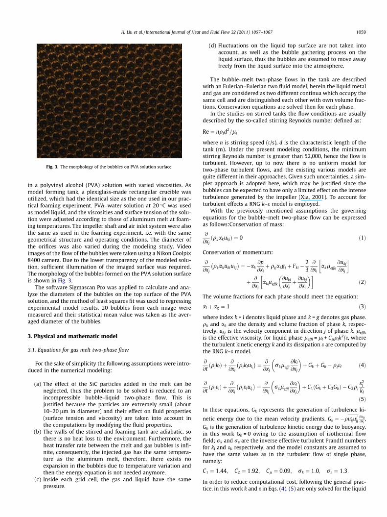
Fig. 3. The morphology of the bubbles on PVA solution surface.

H. Liu et al. / International Journal of Heat and Fluid Flow 32 (2011) 1057–1067 1059

in a polyvinyl alcohol (PVA) solution with varied viscosities. Asmodel forming tank, a plexiglass-made rectangular crucible wasutilized, which had the identical size as the one used in our prac-tical foaming experiment. PVA–water solution at 20 �C was usedas model liquid, and the viscosities and surface tension of the solu-tion were adjusted according to those of aluminum melt at foam-ing temperatures. The impeller shaft and air inlet system were alsothe same as used in the foaming experiment, i.e. with the samegeometrical structure and operating conditions. The diameter ofthe orifices was also varied during the modeling study. Videoimages of the flow of the bubbles were taken using a Nikon Coolpix8400 camera. Due to the lower transparency of the modeled solu-tion, sufficient illumination of the imaged surface was required.The morphology of the bubbles formed on the PVA solution surfaceis shown in Fig. 3.

The software Sigmascan Pro was applied to calculate and ana-lyze the diameters of the bubbles on the top surface of the PVAsolution, and the method of least squares fit was used to regressingexperimental model results. 20 bubbles from each image weremeasured and their statistical mean value was taken as the aver-aged diameter of the bubbles.

3. Physical and mathematic model

3.1. Equations for gas melt two-phase flow

For the sake of simplicity the following assumptions were intro-duced in the numerical modeling:

(a) The effect of the SiC particles added in the melt can beneglected, thus the problem to be solved is reduced to anincompressible bubble–liquid two-phase flow. This isjustified because the particles are extremely small (about10–20 lm in diameter) and their effect on fluid properties(surface tension and viscosity) are taken into account inthe computations by modifying the fluid properties.

(b) The walls of the stirred and foaming tank are adiabatic, sothere is no heat loss to the environment. Furthermore, theheat transfer rate between the melt and gas bubbles is infi-nite, consequently, the injected gas has the same tempera-ture as the aluminum melt, therefore, there exists noexpansion in the bubbles due to temperature variation andthen the energy equation is not needed anymore.

(c) Inside each grid cell, the gas and liquid have the samepressure.

(d) Fluctuations on the liquid top surface are not taken intoaccount, as well as the bubble gathering process on theliquid surface, thus the bubbles are assumed to move awayfreely from the liquid surface into the atmosphere.

The bubble–melt two-phase flows in the tank are describedwith an Eulerian–Eulerian two fluid model, herein the liquid metaland gas are considered as two different continua which occupy thesame cell and are distinguished each other with own volume frac-tions. Conservation equations are solved then for each phase.

In the studies on stirred tanks the flow conditions are usuallydescribed by the so-called stirring Reynolds number defined as:

Re ¼ nqld2=ll

where n is stirring speed (r/s), d is the characteristic length of thetank (m). Under the present modeling conditions, the minimumstirring Reynolds number is greater than 52,000, hence the flow isturbulent. However, up to now there is no uniform model fortwo-phase turbulent flows, and the existing various models arequite different in their approaches. Given such uncertainties, a sim-pler approach is adopted here, which may be justified since thebubbles can be expected to have only a limited effect on the intenseturbulence generated by the impeller (Xia, 2001). To account forturbulent effects a RNG k–e model is employed.

With the previously mentioned assumptions the governingequations for the bubble–melt two-phase flow can be expressedas follows:Conservation of mass:

@

@xjðqkakukjÞ ¼ 0 ð1Þ

Conservation of momentum:

@

@xjqkakukiukj� �

¼ �ak@p@xiþ qkakgi þ Fki �

23@

@xiakleffk

@ukj

@xj

� �

þ @

@xjakleffk

@uki

@xjþ @ukj

@xi

� �� �ð2Þ

The volume fractions for each phase should meet the equation:

al þ ag ¼ 1 ð3Þ

where index k = l denotes liquid phase and k = g denotes gas phase.qk and ak are the density and volume fraction of phase k, respec-tively, ukj is the velocity component in direction j of phase k. leffk

is the effective viscosity, for liquid phase leffl = ll + Clqlk2/e, where

the turbulent kinetic energy k and its dissipation e are computed bythe RNG k–e model.

@

@tqlklð Þ þ @

@xiqlkluli

� �¼ @

@xjrkleffl

@kl

@xj

� �þ Gk þ Gb � qlel ð4Þ

@

@tqlelð Þ þ @

@xiqleluli

� �¼ @

@xjreleffl

@el

@xj

� �þ C1ðGk þ C3GbÞ � C2ql

e2l

kl

ð5Þ

In these equations, Gk represents the generation of turbulence ki-

netic energy due to the mean velocity gradients, Gk ¼ �qu=liu=

lj@ulj

@xi,

Gb is the generation of turbulence kinetic energy due to buoyancy,in this work Gb = 0 owing to the assumption of isothermal flowfield; rk and re are the inverse effective turbulent Prandtl numbersfor kl and el, respectively, and the model constants are assumed tohave the same values as in the turbulent flow of single phase,namely:

C1 ¼ 1:44; C2 ¼ 1:92; Cl ¼ 0:09; rk ¼ 1:0; re ¼ 1:3:

In order to reduce computational cost, following the general prac-tice, in this work k and e in Eqs. (4), (5) are only solved for the liquid

1060 H. Liu et al. / International Journal of Heat and Fluid Flow 32 (2011) 1057–1067

phase, and the effective viscosity of gas phase is estimated from thatof the liquid:

leffg ¼qg

qlleffl

which is an empirical formula widely used in the literature, e.g.Mendez et al. (2005).

In Eq (2) Fki represents the momentum exchange between gasand liquid which consists of several interfacial forces, among themthe drag force between the two phases is dominant. Other forces,such as the virtual mass force and the Saffman force, are not impor-tant in comparison with the drag force and are neglected in thisstudy. The drag force is given by

F!

Dg ¼ �

34qlagal

CD

db~ug �~ul

�� ��ð~ug �~ulÞ ¼ �F!

Dl ð6Þ

where CD and db denote the drag coefficient and bubble diameterrespectively. In the literature there are various formulas for deter-mining the drag coefficient, which are valid usually only under cer-tain flow conditions. These can be basically divided into twocategories: one is dependent mainly on the flow Reynolds numberfrom which one expression frequently used is Schiller andNauman’s:

CD ¼24Re

1þ 0:15Re0:687

The other is dependent on the Eotvos number such as suggestedby Ishii and Zuber (1979), which takes into account the effect ofbubble wake on the drag:

CD ¼ 2=3a2l E0:5

O ð7Þ

where EO ¼ gðql � qgÞd2b=r is the Eotvos number, r is the surface

tension coefficient of the liquid. We carried out numerical experi-ments using both of the formulas for bubble drag coefficient andfound that the latter provided better agreement with measure-ments, so it is employed for the computations in this study. Accord-ing to Ishii and Zuber (1979), for bubbles, especially those withrelative large sizes as considered in this work, the flow regime ischaracterized by the distortion of bubble shapes and irregular mo-tions. In this regime, the experimental data show that the drag forceis governed by distortion and swerving motion of the bubble andindependent of the viscosity, and the change of the bubble shapeis towards an increase in the effective cross section. Therefore, thedrag coefficient should be scaled by the mean diameters of the bub-ble rather than the Reynolds number, and the use of Eq. (7) is jus-tified. The effect of the particles added into the melt on its surfacetension has been taken into account in the computations.

3.2. Model of bubble breakup and coalescence

In our previous study (Liu et al., 2007), bubbles were assumedto be uniform in size. In fact, due to the impeller stirring and liquidturbulence, bubbles breakup inevitably into smaller ones, at thesame time, collision and coalescence of bubbles also take placeduring their moving and rising. Consequently, bubble sizes are fre-quently in variation and, instead of a constant diameter, a distribu-tion of bubble sizes exists in the stirred tank. To predict bubble sizedistribution requires calculation of interfacial area and interphasetransfer of momentum, mass and energy between the melt andbubbles. A full population balance model has been avoided at thisstage since this would add considerably to the computational de-mand. Instead, following Lane et al. (2005), we utilized the modelof bubble number density equation, which allows the prediction ofthe mean bubble diameter at each point in the calculation. The

concept of this approach is based on the bubble number density,n, given by

n ¼ ag

ðp=6Þd3b

ð8Þ

where db is the mean bubble diameter as a function of its location.From the values of n at each point in the tank, the local average bub-ble size db can be calculated.

To determine n we have to solve an additional transport equa-tion accounting for transport of bubbles (by convection and turbu-lent diffusion) and changes in bubble sizes (and therefore bubblenumber) by breakup and coalescence according to

@

@xjðnUg � DnrnÞ ¼ Sbr � Sco ð9Þ

where Sbr and Sco are the source and sink terms of the bubble num-ber density describing the rates of bubble breakup and coalescence,respectively. The diffusivity coefficient, Dn, is assumed to have thesame value as the effective diffusivity coefficient Dlg (Luo et al.,1994)

In modeling coalescence, it is generally considered that coales-cence occurs due to binary collisions between bubbles, and expres-sions for collision rate are derived by assuming random collisionsinduced by turbulent eddies, analogously to the model for molec-ular collisions in the kinetic theory of an ideal gas. Hence the coa-lescence rate term has the following form Lane et al. (2005):

Sco ¼ Ccogcod2b edbð Þ1=3n2 ð10Þ

where gco is the coalescence efficiency, which takes into account thefinite time for bubble deformation and the effect of liquid filmdrainage, and can be written as Kamp et al. (2001).

gco ¼ exp �Kp

ffiffiffiffiffiffiffiffiffiWeCvm

s !ð11Þ

where the dimensionless parameter Kp describes the relationshipbetween the coalescence efficiency and collision frequency, andCvm is a virtual mass coefficient depending on bubble deformationand film drainage time. According to an experimental and numeri-cal study by Kamp et al. (2001), we take the values Kp = 0.9748, andCvm = 0.803.

Bubble breakup is considered to depend on the collisions fre-quency between bubbles and turbulent eddies of similar size,somewhat analogous to the frequency of bubble collisions in thecoalescence model. The tendency of bubbles to break up or remainstable may be defined in terms of the Weber number, i.e., the ratioof the disruptive forces to the restoring surface tension force being

given by We ¼ qu2t dbr . Here, ut is taken to be the velocity of eddies in

the inertial subrange of the turbulent eddy spectrum, which maybe written as ut = 1.4(edb)1/3. Bubble breakup occurs only whenthe Weber number exceeds a critical value, Wecrit, for which differ-ent values (in the range of 1.0–5.0) have been given in the litera-ture. Here it is taken as 1.2 based on a numerical experiment.Furthermore, only a certain fraction of eddies may have sufficientenergy to break up a bubble, and this leads to an efficiency factorin the form of an exponential function. The final expression forthe breakup rate is given by Lane et al. (2005).

Sbr ¼ Cbrnedbð Þ1=3

db1� ag� �

exp �Wecrit

We

� �We > Wecrit ð12Þ

In Eqs. (10) and (12), the coefficients Cco and Cbr are empiricalconstants. Their original values provided by Lane et al. (2005) wereobtained from experiments on a conventional gas–liquid flow in astirred tank, and were found not suitable to the present situation.Based on our PVA solution modeling experiments, a number of

H. Liu et al. / International Journal of Heat and Fluid Flow 32 (2011) 1057–1067 1061

numerical tests were conducted with various values of Cco and Cbr

and the results were compared with experiments. By the best fit-ting the following values were obtained: Cco = 5.64 � 10�9 andCbr = 0.00011. In our PVA–water solution experiments the viscosityand surface tension of the solution were adjusted according tothose of aluminum melt at foaming temperatures to meet the geo-metrical and dynamical similarity between the water model andthe real system. Thus, the above values of the coefficients Cco andCbr can be considered applicable to the cases of air injection intoreal aluminum melt.

3.3. Numerical method

3.3.1. The method of multiple reference framesUp to now, most simulations of stirred tanks have been per-

formed on single-phase flows, and the impeller flow region hasbeen simulated in different ways. In some cases empirical modelsare provided for the impeller. Using a rotating coordinate system isa preferable choice currently for computations of flows in the stir-red tank. There are three different methods in this category. Thefirst two are very similar and are called the Multiple ReferenceFrames method (MRF) and the Inner–outer method (IO) respec-tively. The former was introduced by Luo et al. (1994) and the lat-ter was by Brucato et al. (1998). In the simulations, the equationsfor the fixed and the rotating parts of the geometry are solved sep-arately. There is only one distinct difference between MRF and IO,namely, in IO the calculation domains of the two parts have a smalloverlap. This is not the case for MRF. In the IO method, a number ofouter iterations are required to ensure continuity across the inter-face between the two parts. This implies extra calculation timecompared to the MRF method. The third method using a rotatingcoordinate system is the sliding grid method (SG). This is a time-dependent method where the section of the grid surrounding theimpeller is allowed to rotate stepwise, and the flow field is recalcu-lated for each step. This implies that the simulations need to betransient, hence the computational requirements become exces-sive for the case of two-phase flows, making them computationallymore expensive than the steady state methods. In contrast, theMRF method is a steady-state calculation method with a degreeof accuracy comparable to the sliding mesh method but saving incomputer time greatly.

Based on the above discussion, the Multi-Reference Framemethod is used here. The flow field is calculated by dividing thetank into two domains each with their own frames of reference.In the impeller region flow is calculated in a rotating frame of

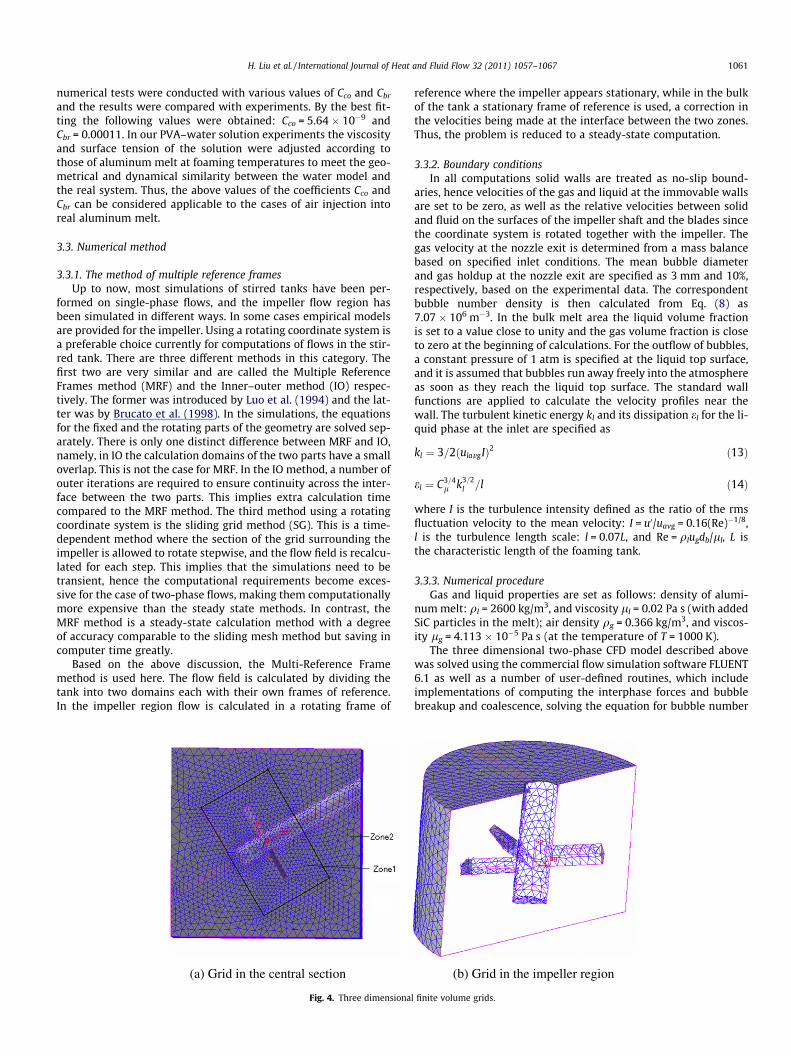
(a) Grid in the central section

Fig. 4. Three dimensiona

reference where the impeller appears stationary, while in the bulkof the tank a stationary frame of reference is used, a correction inthe velocities being made at the interface between the two zones.Thus, the problem is reduced to a steady-state computation.

3.3.2. Boundary conditionsIn all computations solid walls are treated as no-slip bound-

aries, hence velocities of the gas and liquid at the immovable wallsare set to be zero, as well as the relative velocities between solidand fluid on the surfaces of the impeller shaft and the blades sincethe coordinate system is rotated together with the impeller. Thegas velocity at the nozzle exit is determined from a mass balancebased on specified inlet conditions. The mean bubble diameterand gas holdup at the nozzle exit are specified as 3 mm and 10%,respectively, based on the experimental data. The correspondentbubble number density is then calculated from Eq. (8) as7.07 � 106 m�3. In the bulk melt area the liquid volume fractionis set to a value close to unity and the gas volume fraction is closeto zero at the beginning of calculations. For the outflow of bubbles,a constant pressure of 1 atm is specified at the liquid top surface,and it is assumed that bubbles run away freely into the atmosphereas soon as they reach the liquid top surface. The standard wallfunctions are applied to calculate the velocity profiles near thewall. The turbulent kinetic energy kl and its dissipation el for the li-quid phase at the inlet are specified as

kl ¼ 3=2ðulavgIÞ2 ð13Þ

el ¼ C3=4l k3=2

l =l ð14Þ

where I is the turbulence intensity defined as the ratio of the rmsfluctuation velocity to the mean velocity: I = u0/uavg = 0.16(Re)�1/8,l is the turbulence length scale: l = 0.07L, and Re = qlugdb/ll, L isthe characteristic length of the foaming tank.

3.3.3. Numerical procedureGas and liquid properties are set as follows: density of alumi-

num melt: ql = 2600 kg/m3, and viscosity ll = 0.02 Pa s (with addedSiC particles in the melt); air density qg = 0.366 kg/m3, and viscos-ity lg = 4.113 � 10�5 Pa s (at the temperature of T = 1000 K).

The three dimensional two-phase CFD model described abovewas solved using the commercial flow simulation software FLUENT6.1 as well as a number of user-defined routines, which includeimplementations of computing the interphase forces and bubblebreakup and coalescence, solving the equation for bubble number

(b) Grid in the impeller region

l finite volume grids.

1062 H. Liu et al. / International Journal of Heat and Fluid Flow 32 (2011) 1057–1067

density and determining bubble size, etc. In view of the compli-cated configuration due to the inclined stirring shaft and impellerblades, non-uniform structured grids are used as shown in Fig. 4.To determine the optimum mesh size, a mesh independence studywas performed, which showed that computational results changedlittle when the cell number reached 105. Thus, to keep a lowercomputation cost, all simulations of this work are carried out withthe cell number of 105.

For the discretization and solution of variables, a second-orderupwind scheme is applied to the equations of momentum, turbu-lence kinetic energy and turbulence dissipation rate, and the volu-metric fraction equations for gas and liquid are solved with theQUICK scheme. The SIMPLE algorithm for pressure–velocity cou-pling is used for numerical solving the model equations. Convergedsolution is considered to be reached when the residuals of all thevariables are less than 10�5.

Gas–liquid flows were simulated for four different gas flowrates at a fixed impeller rotation speed. In addition, influence ofimpeller rotation speed was examined at a fixed gas flow rate.Unfortunately, very few experimental data are available for a sys-tematic comparison of predicted results with measurement. There-fore, we restrict the scope mainly to qualitative discussions of thepredicted results. Besides, computations were carried out also forPVA–water solution as the liquid phase in the forming tank, so thatthe predicted mean bubble sizes could be compared with datafrom our water model experiments.

4. Results and discussion

4.1. Flow characteristics of liquid phase

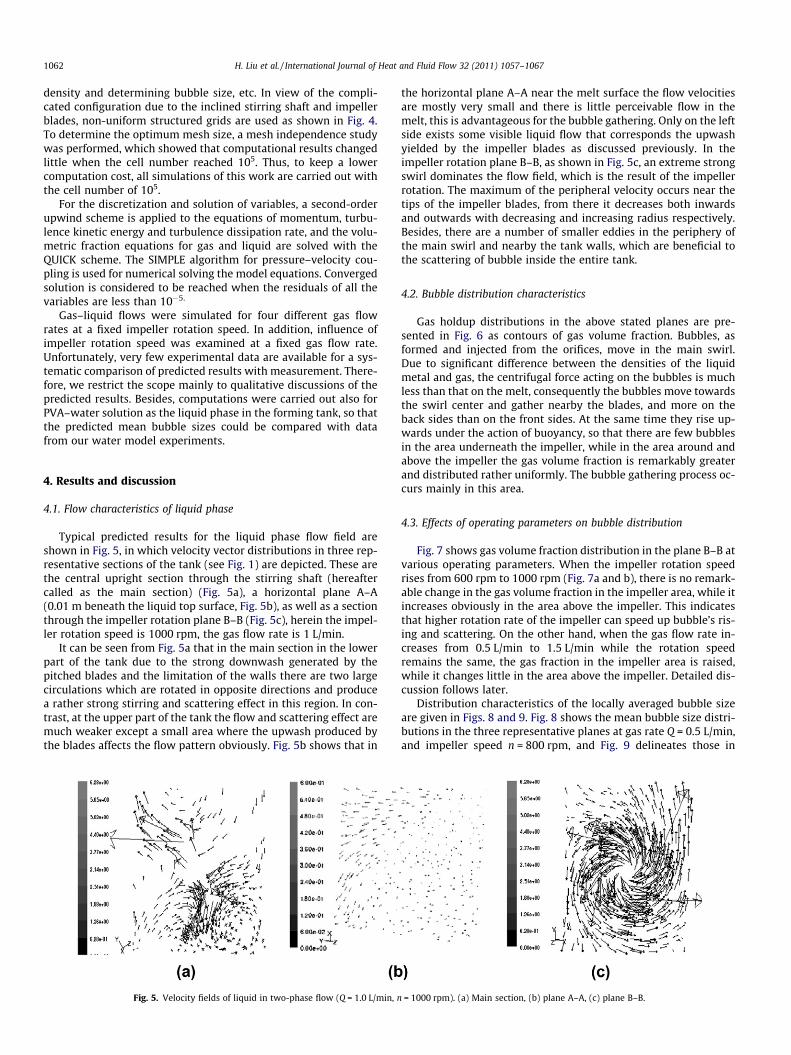
Typical predicted results for the liquid phase flow field areshown in Fig. 5, in which velocity vector distributions in three rep-resentative sections of the tank (see Fig. 1) are depicted. These arethe central upright section through the stirring shaft (hereaftercalled as the main section) (Fig. 5a), a horizontal plane A–A(0.01 m beneath the liquid top surface, Fig. 5b), as well as a sectionthrough the impeller rotation plane B–B (Fig. 5c), herein the impel-ler rotation speed is 1000 rpm, the gas flow rate is 1 L/min.

It can be seen from Fig. 5a that in the main section in the lowerpart of the tank due to the strong downwash generated by thepitched blades and the limitation of the walls there are two largecirculations which are rotated in opposite directions and producea rather strong stirring and scattering effect in this region. In con-trast, at the upper part of the tank the flow and scattering effect aremuch weaker except a small area where the upwash produced bythe blades affects the flow pattern obviously. Fig. 5b shows that in

Fig. 5. Velocity fields of liquid in two-phase flow (Q = 1.0 L/min, n

the horizontal plane A–A near the melt surface the flow velocitiesare mostly very small and there is little perceivable flow in themelt, this is advantageous for the bubble gathering. Only on the leftside exists some visible liquid flow that corresponds the upwashyielded by the impeller blades as discussed previously. In theimpeller rotation plane B–B, as shown in Fig. 5c, an extreme strongswirl dominates the flow field, which is the result of the impellerrotation. The maximum of the peripheral velocity occurs near thetips of the impeller blades, from there it decreases both inwardsand outwards with decreasing and increasing radius respectively.Besides, there are a number of smaller eddies in the periphery ofthe main swirl and nearby the tank walls, which are beneficial tothe scattering of bubble inside the entire tank.

4.2. Bubble distribution characteristics

Gas holdup distributions in the above stated planes are pre-sented in Fig. 6 as contours of gas volume fraction. Bubbles, asformed and injected from the orifices, move in the main swirl.Due to significant difference between the densities of the liquidmetal and gas, the centrifugal force acting on the bubbles is muchless than that on the melt, consequently the bubbles move towardsthe swirl center and gather nearby the blades, and more on theback sides than on the front sides. At the same time they rise up-wards under the action of buoyancy, so that there are few bubblesin the area underneath the impeller, while in the area around andabove the impeller the gas volume fraction is remarkably greaterand distributed rather uniformly. The bubble gathering process oc-curs mainly in this area.

4.3. Effects of operating parameters on bubble distribution

Fig. 7 shows gas volume fraction distribution in the plane B–B atvarious operating parameters. When the impeller rotation speedrises from 600 rpm to 1000 rpm (Fig. 7a and b), there is no remark-able change in the gas volume fraction in the impeller area, while itincreases obviously in the area above the impeller. This indicatesthat higher rotation rate of the impeller can speed up bubble’s ris-ing and scattering. On the other hand, when the gas flow rate in-creases from 0.5 L/min to 1.5 L/min while the rotation speedremains the same, the gas fraction in the impeller area is raised,while it changes little in the area above the impeller. Detailed dis-cussion follows later.

Distribution characteristics of the locally averaged bubble sizeare given in Figs. 8 and 9. Fig. 8 shows the mean bubble size distri-butions in the three representative planes at gas rate Q = 0.5 L/min,and impeller speed n = 800 rpm, and Fig. 9 delineates those in

= 1000 rpm). (a) Main section, (b) plane A–A, (c) plane B–B.

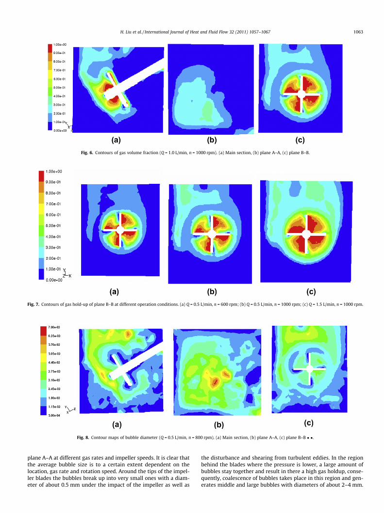
Fig. 6. Contours of gas volume fraction (Q = 1.0 L/min, n = 1000 rpm). (a) Main section, (b) plane A–A, (c) plane B–B.

Fig. 7. Contours of gas hold-up of plane B–B at different operation conditions. (a) Q = 0.5 L/min, n = 600 rpm; (b) Q = 0.5 L/min, n = 1000 rpm; (c) Q = 1.5 L/min, n = 1000 rpm.

Fig. 8. Contour maps of bubble diameter (Q = 0.5 L/min, n = 800 rpm). (a) Main section, (b) plane A–A, (c) plane B–B � �.

H. Liu et al. / International Journal of Heat and Fluid Flow 32 (2011) 1057–1067 1063

plane A–A at different gas rates and impeller speeds. It is clear thatthe average bubble size is to a certain extent dependent on thelocation, gas rate and rotation speed. Around the tips of the impel-ler blades the bubbles break up into very small ones with a diam-eter of about 0.5 mm under the impact of the impeller as well as

the disturbance and shearing from turbulent eddies. In the regionbehind the blades where the pressure is lower, a large amount ofbubbles stay together and result in there a high gas holdup, conse-quently, coalescence of bubbles takes place in this region and gen-erates middle and large bubbles with diameters of about 2–4 mm.

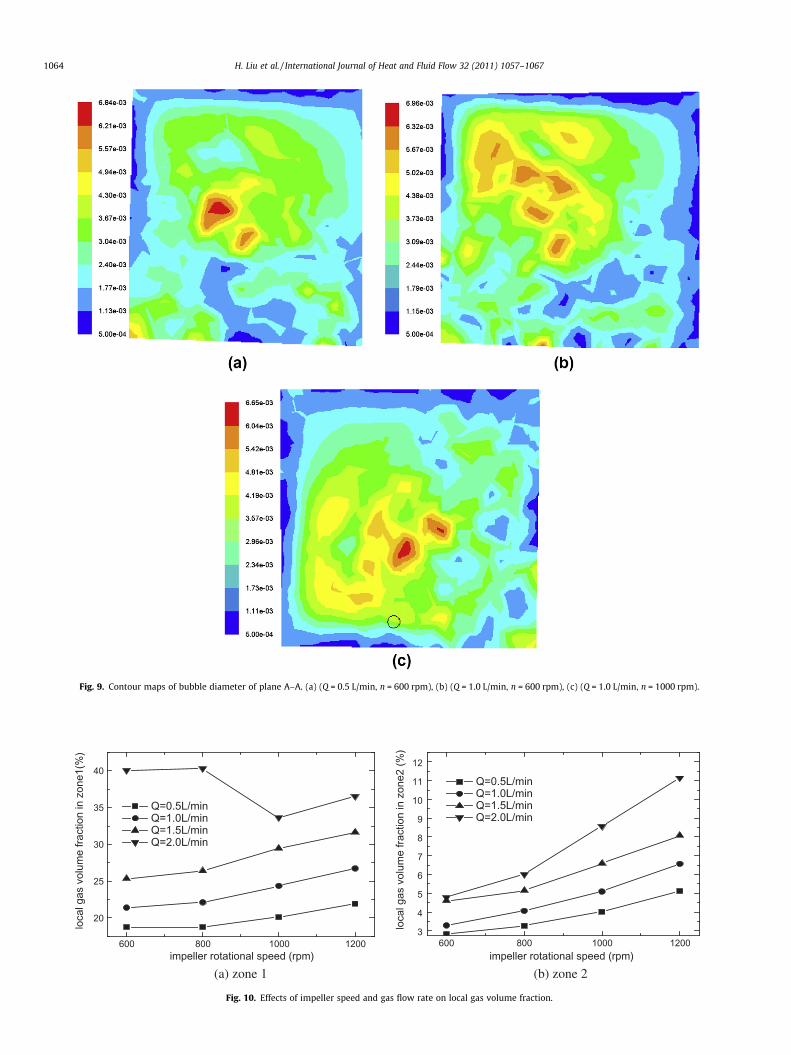
Fig. 9. Contour maps of bubble diameter of plane A–A. (a) (Q = 0.5 L/min, n = 600 rpm), (b) (Q = 1.0 L/min, n = 600 rpm), (c) (Q = 1.0 L/min, n = 1000 rpm).

600 800 1000 1200

20

25

30

35

40

loca

l gas

vol

ume

fract

ion

in z

one1

(%)

impeller rotational speed (rpm)

Q=0.5L/min Q=1.0L/min Q=1.5L/min Q=2.0L/min

600 800 1000 12003

4

5

6

7

8

9

10

11

12

loca

l gas

vol

ume

fract

ion

in z

one2

(%)

impeller rotational speed (rpm)

Q=0.5L/min Q=1.0L/min Q=1.5L/min Q=2.0L/min

(a) zone 1 (b) zone 2

Fig. 10. Effects of impeller speed and gas flow rate on local gas volume fraction.

1064 H. Liu et al. / International Journal of Heat and Fluid Flow 32 (2011) 1057–1067

600 800 1000 12001.9

2.0

2.1

2.2

2.3

2.4

2.5

2.6

2.7

glob

al a

vera

ge b

ubbl

e di

amet

er (m

m)

impeller rotational speed (rpm)

Q=0.5L/min Q=1.0L/min Q=1.5L/min Q=2.0L/min

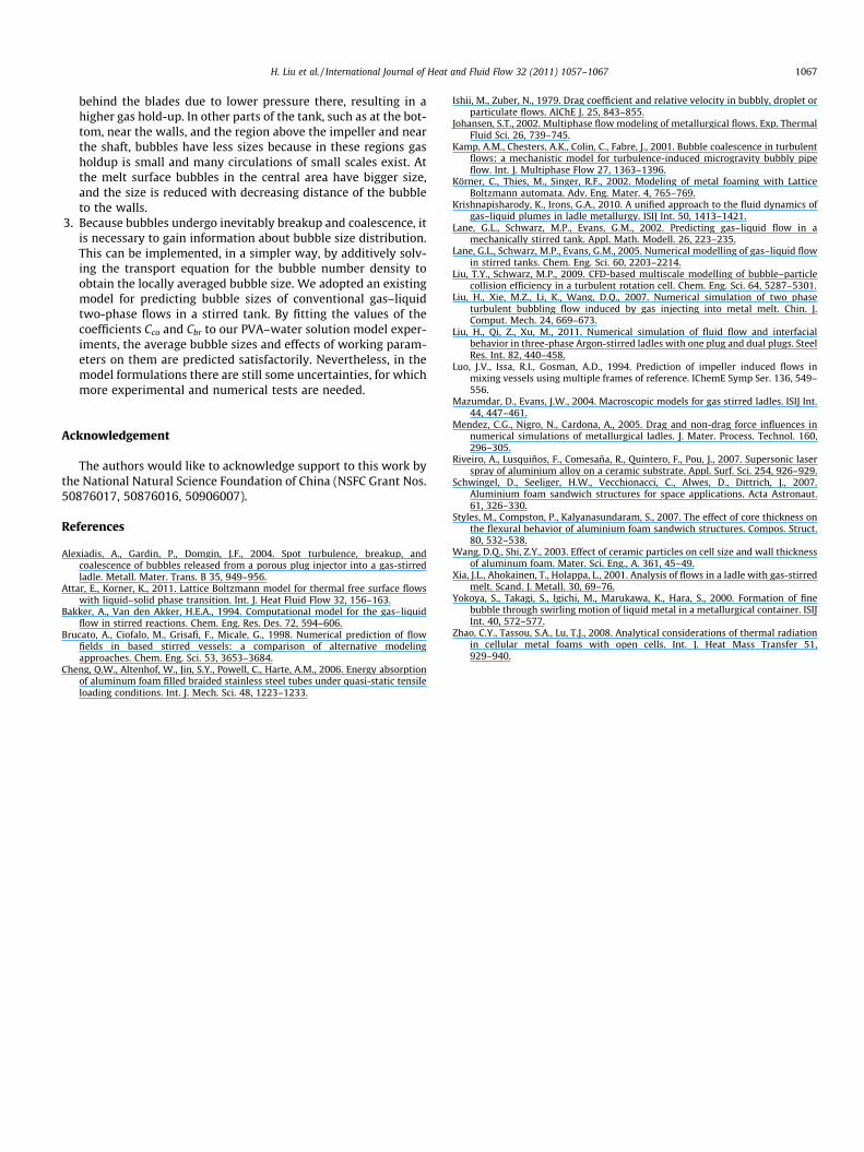
Fig. 13. Effects of impeller speed and gas flow rate and initial bubble diameter onglobal average bubble diameter.

600 800 1000 1200

2.4

2.6

2.8

3.0

3.2

3.4

3.6

3.8

4.0lo

cal a

vera

ge b

ubbl

e di

amet

er in

pla

in A

-A (m

m)

impeller rotational speed (rpm)

Q=0.5L/min Q=1.0L/min Q=1.5L/min Q=2.0L/min

Fig. 14. Effects of impeller speed and gas flow rate on local average bubblediameter in plane A–A.

600 800 1000 12005

6

7

8

9

10

11

12

13

glob

al g

as v

olum

e fra

ctio

n (%

)

impeller rotational speed (rpm)

Q=0.5L/min Q=1.0L/min Q=1.5L/min Q=2.0L/min

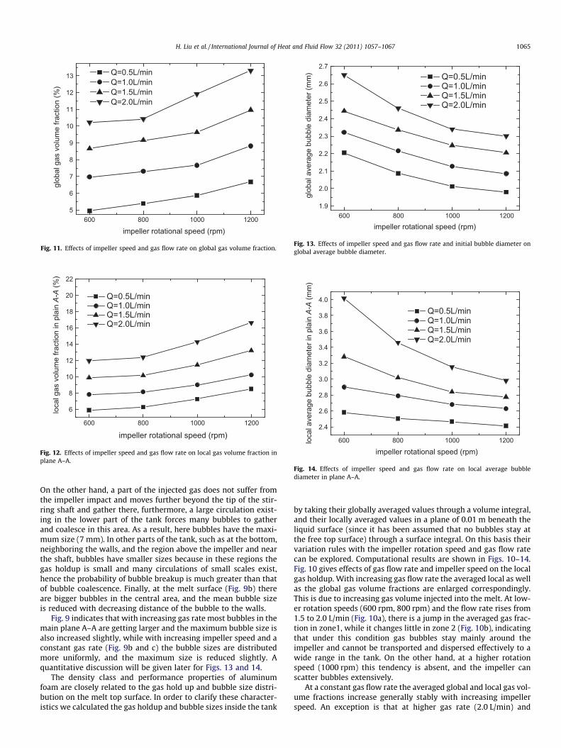
Fig. 11. Effects of impeller speed and gas flow rate on global gas volume fraction.

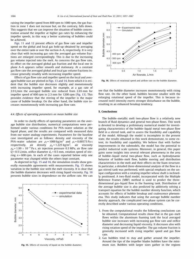
600 800 1000 1200

6

8

10

12

14

16

18

20

22

loca

l gas

vol

ume

fract

ion

in p

lain

A-A

(%)

impeller rotational speed (rpm)

Q=0.5L/min Q=1.0L/min Q=1.5L/min Q=2.0L/min

Fig. 12. Effects of impeller speed and gas flow rate on local gas volume fraction inplane A–A.

H. Liu et al. / International Journal of Heat and Fluid Flow 32 (2011) 1057–1067 1065

On the other hand, a part of the injected gas does not suffer fromthe impeller impact and moves further beyond the tip of the stir-ring shaft and gather there, furthermore, a large circulation exist-ing in the lower part of the tank forces many bubbles to gatherand coalesce in this area. As a result, here bubbles have the maxi-mum size (7 mm). In other parts of the tank, such as at the bottom,neighboring the walls, and the region above the impeller and nearthe shaft, bubbles have smaller sizes because in these regions thegas holdup is small and many circulations of small scales exist,hence the probability of bubble breakup is much greater than thatof bubble coalescence. Finally, at the melt surface (Fig. 9b) thereare bigger bubbles in the central area, and the mean bubble sizeis reduced with decreasing distance of the bubble to the walls.

Fig. 9 indicates that with increasing gas rate most bubbles in themain plane A–A are getting larger and the maximum bubble size isalso increased slightly, while with increasing impeller speed and aconstant gas rate (Fig. 9b and c) the bubble sizes are distributedmore uniformly, and the maximum size is reduced slightly. Aquantitative discussion will be given later for Figs. 13 and 14.

The density class and performance properties of aluminumfoam are closely related to the gas hold up and bubble size distri-bution on the melt top surface. In order to clarify these character-istics we calculated the gas holdup and bubble sizes inside the tank

by taking their globally averaged values through a volume integral,and their locally averaged values in a plane of 0.01 m beneath theliquid surface (since it has been assumed that no bubbles stay atthe free top surface) through a surface integral. On this basis theirvariation rules with the impeller rotation speed and gas flow ratecan be explored. Computational results are shown in Figs. 10–14.Fig. 10 gives effects of gas flow rate and impeller speed on the localgas holdup. With increasing gas flow rate the averaged local as wellas the global gas volume fractions are enlarged correspondingly.This is due to increasing gas volume injected into the melt. At low-er rotation speeds (600 rpm, 800 rpm) and the flow rate rises from1.5 to 2.0 L/min (Fig. 10a), there is a jump in the averaged gas frac-tion in zone1, while it changes little in zone 2 (Fig. 10b), indicatingthat under this condition gas bubbles stay mainly around theimpeller and cannot be transported and dispersed effectively to awide range in the tank. On the other hand, at a higher rotationspeed (1000 rpm) this tendency is absent, and the impeller canscatter bubbles extensively.

At a constant gas flow rate the averaged global and local gas vol-ume fractions increase generally stably with increasing impellerspeed. An exception is that at higher gas rate (2.0 L/min) and

0.5 1.0 1.5 2.0

3.5

4.0

4.5

5.0

5.5

6.0

6.5

Experimental data Simulation

600 rpm

500 rpm

400 rpm

Bubb

le d

iam

eter

,mm

Air flowrate, L/min

Fig. 16. Effects of rotational speed and airflow rate on the bubble diameter.

1066 H. Liu et al. / International Journal of Heat and Fluid Flow 32 (2011) 1057–1067

raising the impeller speed from 800 rpm to 1000 rpm, the gas frac-tion in zone 1 does not increase but, on the contrary, falls down.This suggests that we can improve the situation of bubble concen-tration around the impeller at higher gas rates by enhancing theimpeller speeds, in this way a better scattering of bubbles couldbe achieved.

Figs. 11 and 12 present effects of gas flow rate and impellerspeed on the global and local gas hold-up obtained by averagingover the entire tank or over the section A–A, respectively. It is veryclear that with increasing gas rate the averaged gas volume frac-tions are enlarged correspondingly. This is due to the increasinggas volume injected into the melt. As concerns the gas flow rate,its effect on the averaged global gas fraction and the local one inplane A–A appears rather smooth and stationary. At a constantgas flow rate the averaged global and local gas volume fractions in-crease generally steadily with increasing impeller speed.

Effects of gas flow rate and impeller speed on the local and aver-aged bubble size are plotted in Figs. 13 and 14, from which it is evi-dent that the bubble size decreases slightly and monotonouslywith increasing impeller speed, for example, at a gas rate of2.0 L/min the averaged bubble size reduced from 2.65 mm forimpeller speed of 600 rpm to 2.3 mm for 1200 rpm (Fig. 13). Thisprovides evidence that the stirring of the impeller is the majorcause of bubble breakup. On the other hand, the bubble size in-creases monotonously with increasing gas flow rate.

4.4. Effects of operating parameters on mean bubble size

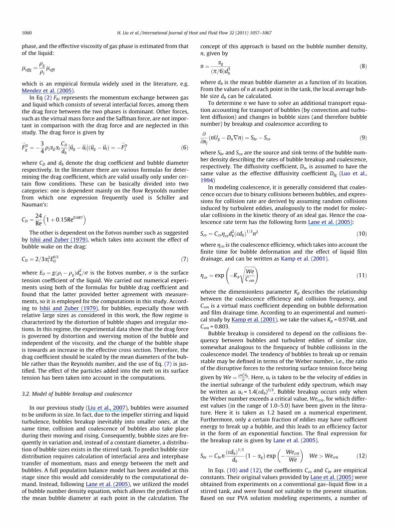
In order to clarify effects of operating parameters on the aver-age bubble size distribution, numerical computations were per-formed under various conditions for PVA–water solution as theliquid phase, and the results are compared with measured datafrom our water analogy experiments. Parameters for the baselinecase investigated are as follows: density and viscosity of thePVA–water solution are qf = 1000 kg/m3 and ll = 0.00573 Pa srespectively, air density qg = 1.225 kg/m3, air viscositylg = 1.99 � 10�5 Pa s, air injection pressure 0.3 MPa, air flow rateQ = 0.5 L/min, orifice diameter do = 0.5 mm, rotation speed of stir-ring n = 600 rpm. In each of the cases reported below only oneparameter was changed while the others kept constant.

As depicted in Figs. 15 and 16, the simulation results show gen-erally reasonable agreements with measurements. Fig. 15 showsvariation in the bubble size with the melt viscosity. It is clear thatthe bubble diameter decreases with rising liquid viscosity. Fig. 16presents bubble sizes in dependence on the airflow rate. We can

3 4 5 6 7 8 9 10 112.0

2.5

3.0

3.5

4.0

4.5

5.0

Bubb

le d

iam

eter

, mm

Viscosity, mPaS

experimental data simulation

Fig. 15. Effects of viscosity of liquid on the bubble diameter.

see that the bubble diameter increases monotonously with risingflow rate. On the other hand, bubbles become smaller with theenlarging rotational speed of the impeller. This is because in-creased swirl intensity exerts stronger disturbance on the bubble,resulting in an enhanced breakup tendency.

5. Conclusions

The bubble–metallic melt two-phase flow is a relatively newbranch of fluid dynamics and general two-phase flows. This workis devoted to develop a preliminary numerical model for investi-gating characteristics of the bubble–liquid metal two-phase flowfield in a stirred tank, and to assess the feasibility and capabilityof the model. Although the model is incomplete in the presentstate, the results obtained in this work demonstrate, to some ex-tent, its feasibility and capability. We believe that with furtherimprovements in the submodels, the model has the potential topredict industrial scale systems. Moreover, in general, this papergains some insights into several relevant phenomena in the areaof bubble–liquid metal two-phase flow, such as hydrodynamicbehavior of bubble–melt flow, bubble moving and distributioncharacteristics in the melt and their effects on the foam structure.In particular, a detailed three-dimensional analysis of the flow in agas stirred tank was performed, with special emphasis on the un-ique configuration with a rotating impeller whose shaft is inclined-ly positioned. A two-fluid model, incorporated with the MultipleReference Frames (MRF) method is used to predict the three-dimensional gas–liquid flow in the foaming tank. Distribution ofthe average bubble size is also predicted by additively solving atransport equation for the bubble number density function, whichaccounts for effects of bubble breakup and coalescence phenom-ena. This study indicates that using the average bubble numberdensity approach, the complicated two-phase system can be cor-rectly described under various operating conditions.

1. From the computational results the following conclusions canbe obtained. Computational results show that in the gas–meltflows within the aluminum foaming tank the local averagedbubble size increases with increasing gas flow rate and orificediameter and decreasing liquid viscosity. It decreases also withrising rotation speed of the impeller. The gas volume fraction isgenerally increased with rising impeller speed and gas flowrate.

2. Gas bubbles tend to stay and gather around the impeller.Around the tips of the impeller blades bubbles have the mini-mum size. Bubbles with larger sizes gather in the regions

H. Liu et al. / International Journal of Heat and Fluid Flow 32 (2011) 1057–1067 1067

behind the blades due to lower pressure there, resulting in ahigher gas hold-up. In other parts of the tank, such as at the bot-tom, near the walls, and the region above the impeller and nearthe shaft, bubbles have less sizes because in these regions gasholdup is small and many circulations of small scales exist. Atthe melt surface bubbles in the central area have bigger size,and the size is reduced with decreasing distance of the bubbleto the walls.

3. Because bubbles undergo inevitably breakup and coalescence, itis necessary to gain information about bubble size distribution.This can be implemented, in a simpler way, by additively solv-ing the transport equation for the bubble number density toobtain the locally averaged bubble size. We adopted an existingmodel for predicting bubble sizes of conventional gas–liquidtwo-phase flows in a stirred tank. By fitting the values of thecoefficients Cco and Cbr to our PVA–water solution model exper-iments, the average bubble sizes and effects of working param-eters on them are predicted satisfactorily. Nevertheless, in themodel formulations there are still some uncertainties, for whichmore experimental and numerical tests are needed.

Acknowledgement

The authors would like to acknowledge support to this work bythe National Natural Science Foundation of China (NSFC Grant Nos.50876017, 50876016, 50906007).

References

Alexiadis, A., Gardin, P., Domgin, J.F., 2004. Spot turbulence, breakup, andcoalescence of bubbles released from a porous plug injector into a gas-stirredladle. Metall. Mater. Trans. B 35, 949–956.

Attar, E., Korner, K., 2011. Lattice Boltzmann model for thermal free surface flowswith liquid–solid phase transition. Int. J. Heat Fluid Flow 32, 156–163.

Bakker, A., Van den Akker, H.E.A., 1994. Computational model for the gas–liquidflow in stirred reactions. Chem. Eng. Res. Des. 72, 594–606.

Brucato, A., Ciofalo, M., Grisafi, F., Micale, G., 1998. Numerical prediction of flowfields in based stirred vessels: a comparison of alternative modelingapproaches. Chem. Eng. Sci. 53, 3653–3684.

Cheng, Q.W., Altenhof, W., Jin, S.Y., Powell, C., Harte, A.M., 2006. Energy absorptionof aluminum foam filled braided stainless steel tubes under quasi-static tensileloading conditions. Int. J. Mech. Sci. 48, 1223–1233.

Ishii, M., Zuber, N., 1979. Drag coefficient and relative velocity in bubbly, droplet orparticulate flows. AIChE J. 25, 843–855.

Johansen, S.T., 2002. Multiphase flow modeling of metallurgical flows. Exp. ThermalFluid Sci. 26, 739–745.

Kamp, A.M., Chesters, A.K., Colin, C., Fabre, J., 2001. Bubble coalescence in turbulentflows: a mechanistic model for turbulence-induced microgravity bubbly pipeflow. Int. J. Multiphase Flow 27, 1363–1396.

Körner, C., Thies, M., Singer, R.F., 2002. Modeling of metal foaming with LatticeBoltzmann automata. Adv. Eng. Mater. 4, 765–769.

Krishnapisharody, K., Irons, G.A., 2010. A unified approach to the fluid dynamics ofgas–liquid plumes in ladle metallurgy. ISIJ Int. 50, 1413–1421.

Lane, G.L., Schwarz, M.P., Evans, G.M., 2002. Predicting gas–liquid flow in amechanically stirred tank. Appl. Math. Modell. 26, 223–235.

Lane, G.L., Schwarz, M.P., Evans, G.M., 2005. Numerical modelling of gas–liquid flowin stirred tanks. Chem. Eng. Sci. 60, 2203–2214.

Liu, T.Y., Schwarz, M.P., 2009. CFD-based multiscale modelling of bubble–particlecollision efficiency in a turbulent rotation cell. Chem. Eng. Sci. 64, 5287–5301.

Liu, H., Xie, M.Z., Li, K., Wang, D.Q., 2007. Numerical simulation of two phaseturbulent bubbling flow induced by gas injecting into metal melt. Chin. J.Comput. Mech. 24, 669–673.

Liu, H., Qi, Z., Xu, M., 2011. Numerical simulation of fluid flow and interfacialbehavior in three-phase Argon-stirred ladles with one plug and dual plugs. SteelRes. Int. 82, 440–458.

Luo, J.V., Issa, R.I., Gosman, A.D., 1994. Prediction of impeller induced flows inmixing vessels using multiple frames of reference. IChemE Symp Ser. 136, 549–556.

Mazumdar, D., Evans, J.W., 2004. Macroscopic models for gas stirred ladles. ISIJ Int.44, 447–461.

Mendez, C.G., Nigro, N., Cardona, A., 2005. Drag and non-drag force influences innumerical simulations of metallurgical ladles. J. Mater. Process. Technol. 160,296–305.

Riveiro, A., Lusquiños, F., Comesaña, R., Quintero, F., Pou, J., 2007. Supersonic laserspray of aluminium alloy on a ceramic substrate. Appl. Surf. Sci. 254, 926–929.

Schwingel, D., Seeliger, H.W., Vecchionacci, C., Alwes, D., Dittrich, J., 2007.Aluminium foam sandwich structures for space applications. Acta Astronaut.61, 326–330.

Styles, M., Compston, P., Kalyanasundaram, S., 2007. The effect of core thickness onthe flexural behavior of aluminium foam sandwich structures. Compos. Struct.80, 532–538.

Wang, D.Q., Shi, Z.Y., 2003. Effect of ceramic particles on cell size and wall thicknessof aluminum foam. Mater. Sci. Eng., A. 361, 45–49.

Xia, J.L., Ahokainen, T., Holappa, L., 2001. Analysis of flows in a ladle with gas-stirredmelt. Scand. J. Metall. 30, 69–76.

Yokoya, S., Takagi, S., Igichi, M., Marukawa, K., Hara, S., 2000. Formation of finebubble through swirling motion of liquid metal in a metallurgical container. ISIJInt. 40, 572–577.

Zhao, C.Y., Tassou, S.A., Lu, T.J., 2008. Analytical considerations of thermal radiationin cellular metal foams with open cells. Int. J. Heat Mass Transfer 51,929–940.