A C T U A R I A L RESEARCH C L E A R I N G H O U S E 1 9 8 4 VOL. 1

Transformation of Grouped Data to Near Normality

Victor M. Guerrero and Richard A. Johnson

I . Introduction

Data may only be available in grouped form because

( i ) Observations are deemed confidential as is the case

with certain economic and sociological information.

( i l ) Respondents to a question check the box corresponding

to an appropriate interval of age, income or other

quantitative variable.

The conventional way to analyze grouped observations on a single

variable is to construct histograms or, sometimes, f i t a normal d i s t r i -

bution. We extend this la t te r approach by allowing for transformations

to near normality.

Typically, transformations have been used to improve the agre~nent

between data and the assumption of normality. Tukey (1977) gives

several reasons for re-expressing data on transformed scale. His

approach i s to t ry a few selections from the transformation ladder

- x - = - , - Z,- , log(xX~, x 2

and then to choose the one that gives the most normal looking graph.

Box and Cox (1964) consider the family of transformations

"j . if o

x ~ ) l

l [log(x), i? x - o

( I )

which applies to non-negative observations. Using this family, which is

continuous in the power k , they present an analytical method for

selecting I .

-153-

In this paper, we investigate transformations to near normality

from grouped data. When the normal approximation is adequate for the

transformed data, we achieve

(i) A simple description in terms of mean and variance.

( l i ) A smoothing of the data.

When the original observations are available, they should be used

in the analysis. Even when there are a large number of cel ls, several

methods of smoothing are available. Our methods wi l l be of primary

Interest when there are re lat ively few cells and the sample size is

moderate.

Out development is given in Section 2. An example appears in

Section 3. Computational details are treated in Section 4 and large

sample properties in Section 5. Section 6 presents an extension to

l i f e tables.

-154-

2. A Transformation of Grouped Data

The problem treated here is that of obtaining the Maximum

Likelihood Estimator'(MLE) when the original random variables

are unobserved and the only available information is the number of

observations fa l l ing within arbitrary, but specified, intervals of the

real l ine.

Let us consider a random sample XI, . . . ,X n from an absolutely

continuous distr ibution with probabil i ty density function (pdf) concen-

trated on (0,®).

The sample wi l l be grouped into k(k ~3) prespecified intervals

denoted by D l = [ao,al), D 2 = [al,a2) . . . . . D k = [ak. l ,a k) where

0 = a 0 < a I < --- < ak. l < a k - ~ The count of the number of obser-

rations in interval D i w i l l be denoted by n i , and the total sample k

size is n - ~ n i . I I

In order to obtain the MLE of (W,o,~) we tentat ively assume that

there exists some i0 such that

{ x o-I , Xo O ~0

x~ x°) : ~21 log (xj), x 0 - o

has a normal distr ibut ion. This assumption cannot hold s t r i c t l y ,

except possibly for LO = O, because Xj is positive.

Under the normal assumption, with ~ ~ O,

-155-

P[X 1 (D i ] - P[al_ l ~ X 1 < a I ]

x)-, ,).l • P[--~ < T < T ]

a (x) u (x) ¢ ( _ ~ [ ~ ) - ,a l - l 'U,

where

" Pl (u,o,k) (3)

a ) - I alk) :, ~ , i f X # 0

l o g ( a i ) , i f k = 0

i : 1,2 . . . . k - I

z

~(z) - S

a (x)

We take po(~,o,X ) . ,(~_T_~)

fo r X a O. For nega t ive X,

The counts (nl,n 2 . . . . . n k)

whose p r o b a b i l i t i e s are s p e c i f i e d in (3) .

z ] e'UZ/2 I d. = (~(u)d-

. a(X)_~ and pk(u,o,X) - l - @(~-~-~)

(x) a(X)_u . ,a i - l 'U , _ ~(~) •

Pi (u,o,X) = ~t---~---)

then have the multinomial distribution

The log-likelihood becomes

Zn(U,o,I) = log(n{) - k k [ log(.i!) + 2

i=l i=] n i log[p i (U,~,X)] (4)

-156-

We choose to maximize the Iog-likellhood using a two-stage

procedure.

Step l : Fix ~ and maximize JLn(l~,~,~) with respect

to p and ~. This yields en(k)-(~n(X),

ancx),x). Step 2: Maximize ILn(en(),)) with respect to X. This

yields the MLE's @n " (~n'Gn'~n)''

In practice, we obtain ~n(k), ~n(L) by solving

- a(),) a(~L)

n

L T,T.,t Z : =0

(s)

~e.n(U,o,X) k n i

~<~- 1 "6"

a(X) , a(x) a(X) a(~) I "~ i - I "$J I -u i - I "~

Pt (~'~'x) ] - 0

where n~erator terms involving a~ ~) and a~ ~) are zero.

-157-

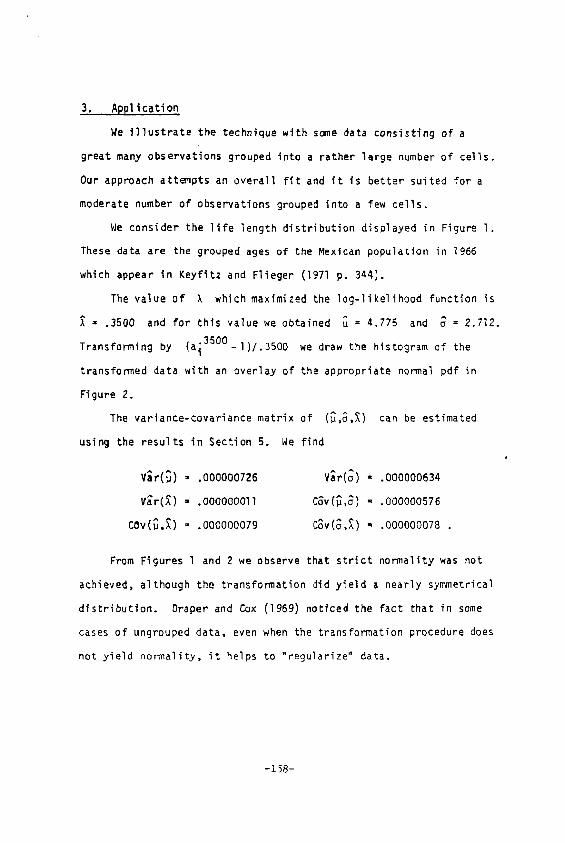
3. Application

We i l l us t ra te the technique with some data consisting of a

great many observations grouped into a rather large number of cells.

Our approach attempts an overall f i t and i t is better suited for a

moderate number of observations grouped into a few cells.

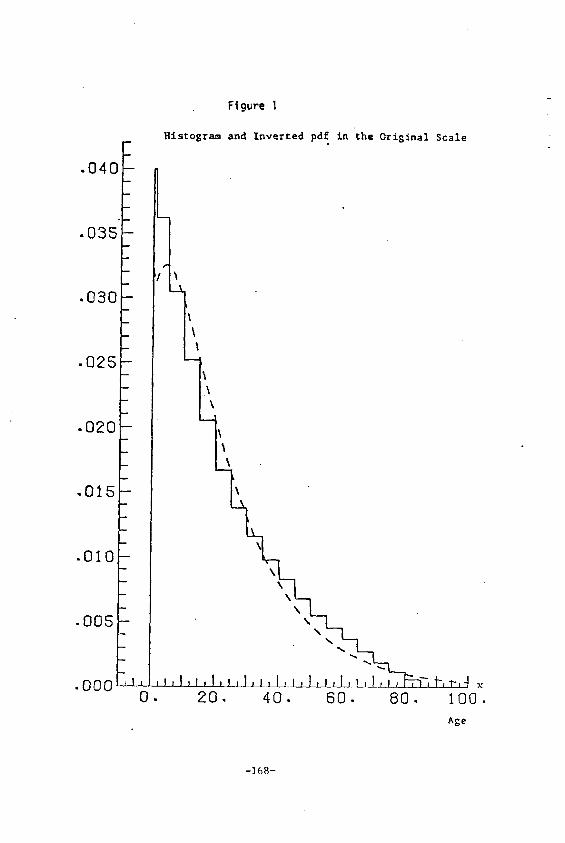
We consider the l i f e length distribution displayed in Figure I.

These data are the grouped ages of the Mexican population in 1966

which appear in Keyfitz and Flieger (1971 p. 344).

The value of k which maximized the log-l ikel ihood Function is

= .3500 and for this value we obtained u = 4.775 and ~ = 2.712.

Transforming by (ai 3500-I)/.3500 we draw the histogram of the

transformed data with an overlay of the appropriate normal pdf in

Figure 2.

The variance-covariance matrix of (~,$,~) can be estimated

using the results in Section 5. We find

V~r(~) - .000000726 Var(;) = .000000634

V~r(~) - .O00000011 CSv(~,~) = .000000576

COv(;,~) = .000000079 C~v(~,~) - .000000078 .

From Figures l and 2 we observe that s t r i c t normality was not

achieved, although the transformation did yield a nearly symmetrical

d istr ibut ion. Draper and Cox (196g) noticed the Fact that in some

cases of ungrouped data, even when the transformation procedure does

not yield normality, i t helps to "regularize" data.

-158-

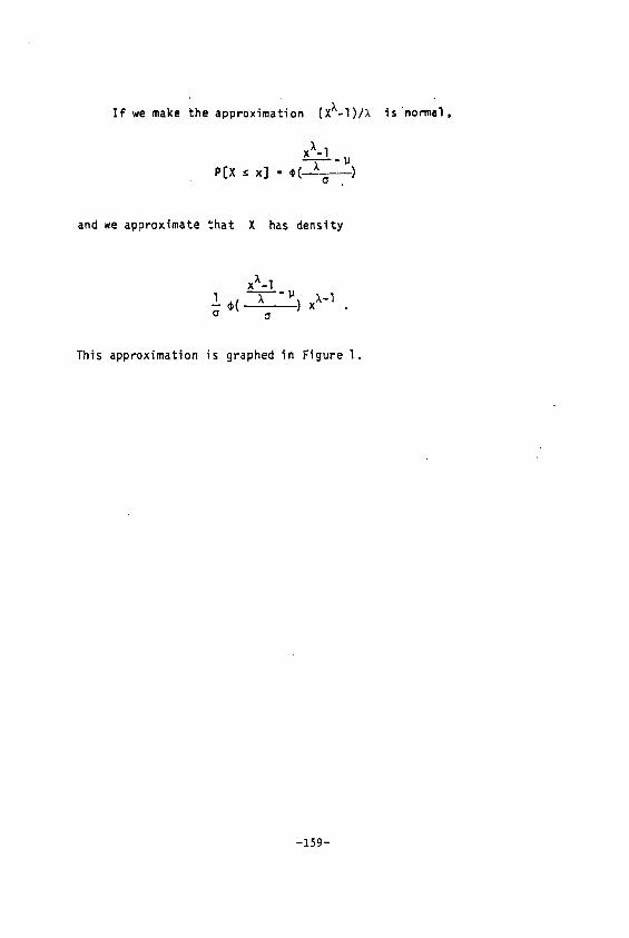
I f we make the approximation (X}'-l)/l is 'normal,

x~_l P[X S X] = ¢ ( - - ~ )

and we approximate that X has density

x~'_l 1 ~ - u.) x-I

o

This approximation is graphed in Figure I.

-159-

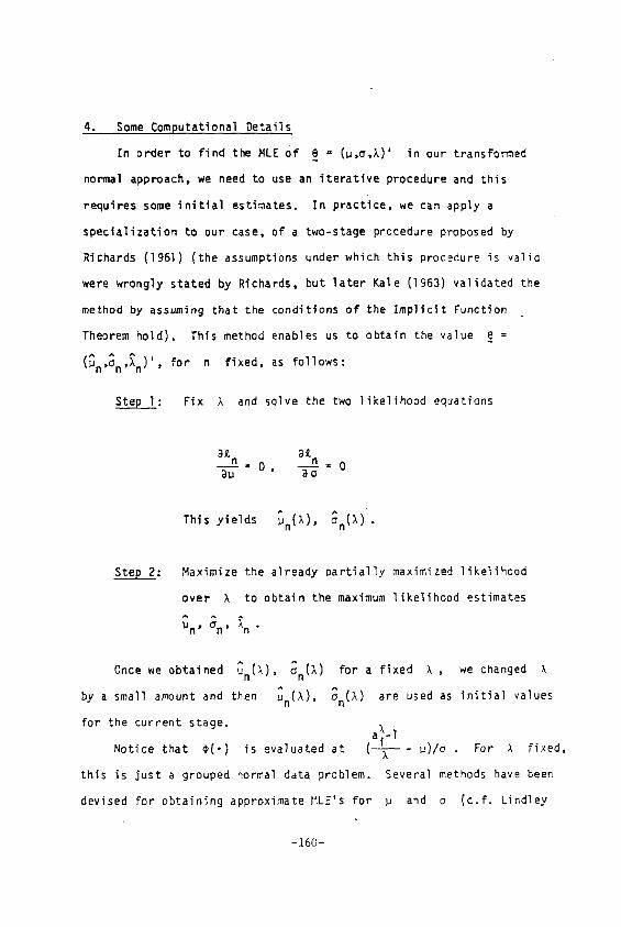
4. Some Computational Details

In order to f ind the MLE Of 8 = (u ,o , l ) ' in our transformed

normal approach, we need to use an i terat ive procedure and this

requires some i n i t i a l estimates. In practice, we can apply a

specialization to our case, of a two-stage procedure proposed by

Richards {1961) (the assumptions under which this procedure is valid

were wrongly stated by Richards, but later Kale (1963) validated the

method by assuming that the conditions of the Impl ic i t Function

Theorem hold). This method enables us to obtain the value 8 =

(~n,~n,~n)', for n fixed, as follows:

Step l : Fix ~ and solve the two l ikel ihood equations

a£ 8£ n_=o, n .= o

au ~) o

" ~, ^ This yields Un ( ) , On(k) .

Step 2: Maximize the already par t ia l l y maximized l ikel ihood

over X to obtain the maximum l ikel ihood estimates ^ ^ ^

Un2 ~n ~ X n •

A

Once we obtained Un(X), On(X) for a fixed X, we changed

by a small amount and then in(X), ~n(X) are used as i n i t i a l values

for the current stage, a~-l

Notice that ¢(-) is evaluated at ( - -~--- u)/o . For ~ fixed,

this is just a grouped normal data problem. Several methods have been

devised for obtaining approximate MLE's for ~ and o (c . f . Lindley

-160-

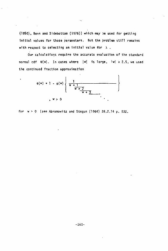
(1950), Benn and Sidebottom (1976)) which may be used for getting

i n i t i a l values for those parameters. But the problem s t i l l remains

with respect to selecting an i n i t i a l value for ~ .

Our calculations require the accurate evaluation of the standard

normal cdf ¢(w). In cases where lwl is large, lwl m 2.5, we used

the continued fraction approximation

t 1 t ¢(w) ~ 1 - ¢(w) w + l

w + 2 w + 3

w > o

for w > 0 (see Abramowitz and Stegun (1964) 26.2.14 p. 932.

-161-

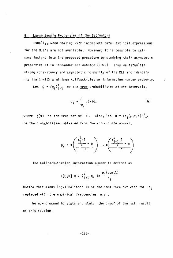
5. Large Sample Properties o f the Estimators

Usually, when dealing with incomplete data, exp l i c i t expressions

for the MLE's are not available. However, i t is possible to gain

some insight into the proposed procedure by studying their asymptotic

properties as in Herna/~dez and Johnson (1979). Thus we establish

strong consistency and asymptotic normality of the r~LE and ident i fy

i ts l im i t with a minimum Kullback-Liebler information number property.

Let Q : {qi}~=l be the true probabil i t ies of the intervals,

: F. g(x)dx (6) qi 'D 1

g(x) is the true pdf of X. Also, let N = {pi(~,~,X)}~= l where

be the probabi l i t ies obtained from the approximate normal,

Pi .@ - - ~ - IJ . _ _

The Ku]Iback-Liebler information number is defined as

Pi (~,~,X) I[Q,N] = - ~i=l qi In

qi

Notice that minus log-l ikel ihood is of the same form but with the qi

replaced with the empirical frequencies ni /n.

We now proceed to state and sketch the proof of the main result

of this section.

- 1 6 2 -

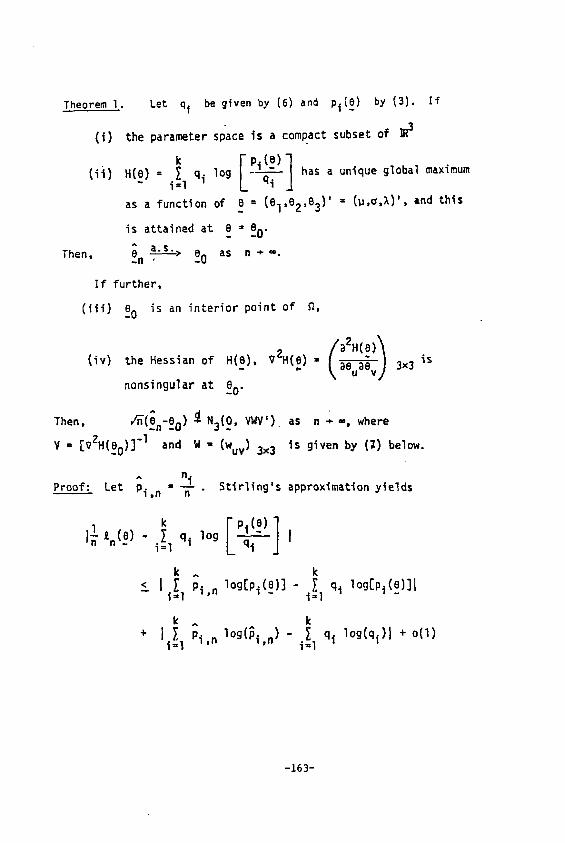
Theorem I. Let ql be given by (6) and pi(~) by (3). I f

( i ) the parameter space is a compact subset of ~3

k F pi( )l ( i i ) H(B) = ~ qi log has a unique global maximum - i-1 L - - ~ ~

as a function of . B : {BI,B2,B3)' = (~,o,X)', and this

is attained at 8 = ~0"

a . s . > B as n ÷ - Then, n ' 0 "

I f further,

( i i i ) ~0 is an interior point of ~,

(iv) the Hessian of H(61,. V2H(~). " k ~ ) 3x3 is

nonsingular at ~0"

Then, ~(Gn_eO) d NsCO ' V~' ) as , + - , where

V = [92H(Bo)]-I and W- (Wuv) 3x3 is givenby (~) below.

^ n I Proof: Let Pi,n = -n" Stir l ing's approximation yields

I~ ~.(~) -

<

i~1 qi log L qt j l

k ~ k

I i~l Pi,n 1og[p~(e)]. " i~I qi 1°gZPi(e)]l.

k k

+ J~ I. Pi,n 1°g(Pi,n) - i=I ~ qi 1°g(qi)l +°(I)

-163-

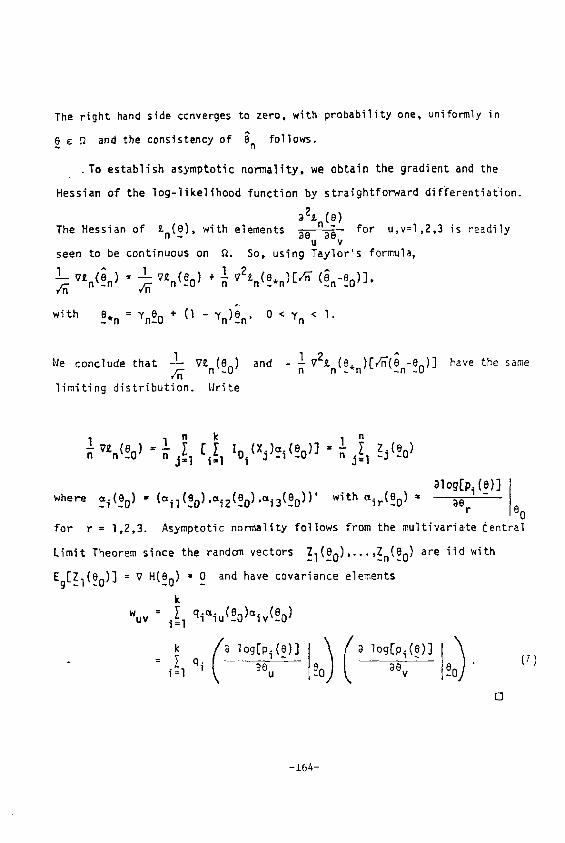
The right hand side converges to zero, with probability one, uniformly in

~ D and the consistency of Bn follows.

. To establish asymptotic normality, we obtain the gradient and the

Hessian of the log-likelihood function by straightforward differentiation.

~2£n(~) The Hessian of ~n(8),_ with elements BB B8 for u,v=l,2,3 is readily

u v seen to be continuous on ~. So, using Taylor's formula,

]__V£n(~n ) : I_]_ I VZ£n(e.n)[/~ (~n.%) ] v~ - VF V~n(~0) + ~ - - - " p.

with ~*n:Yn~O + ( l - ~ n ) ~ . , 0 < ~ n < I .

tVe conclude that I_]_~ 9£n(%) and - nl 92£n(O.n)[~r~(~n_O0) ] ~ _ _

l imit ing d is t r ibu t ion . Write

have the same

lwn(eo) 1 n k 1 i Zj(e o) ~ ~ j-~l [ [ Zoi(Xj)%(_%)] : ~ j : l

alog[p i(@)] 80 where =i(eO) - (mil(%),=i2(Bo),~i3(%))' with air(e O) . . . . aO r

for r = 1,2,3. Asymptotic normality follows from the multivariate Central

Limit Theorem since the random vectors Zl(eO) . . . . . Zn(e0) are i id with

Eg[Zl(90)] = V H(%) = 0 and have covariance elements

k WUV = [ i : l

k

i=l

qi~iu(_%)miv(_ %)

g l°g[Pi(-B)] [ 01 gO v 0 "

[]

(7)

-164-

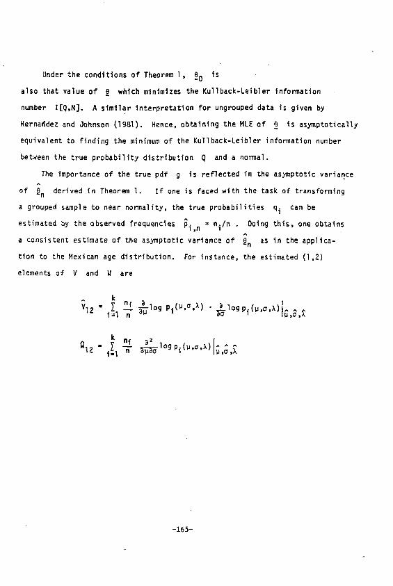
Under the conditions of Theorem l , 20 is

also that value of O which minimizes the Kullback-Leibler information

number I[Q,N]. A similar interpretation for ungrouped data is given by

Herna~dez and Johnson (1981). Hence, obtaining the biLE of e is asymptotically

equivalent to finding the minimum of the Kullback-Leibler information number

between the true probability distribution Q and a normal.

The importance of the true pdf g is reflected in the asymptotic variance

of % derived in Theorem I. I f one is faced with the task of transforming ~n

a grouped sample to near normality, the true probabilities qi can be

estimated by the observed frequencies Pl,n = ni/n " Doing this, one obtains ^

a consistent estimate of the asymptotic variance of ~n as in the applica-

tion to the Mexican age distribution. For instance, the estimated (1,2)

elements of V and W are

k VI2 = 2 ni Bl " I i=l -"- ~ og Pl(U,a, ~) ~o l°g pi(U'a')') ~,8,~

k ni ~)2 [ QI2 = i~l ~ l~l°l°gPi("'cr'X) ~'J'~

-165-

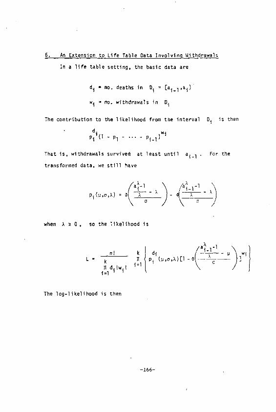
6. An Extension to Life Table Data Involvinq Withdrawals

In a l i fe table setting, the basic data are

d i - no. deaths in D i : [ai_l,a i)

w i - no. withdrawals in D i

The contribution to the likelihood from the interval D i

d i _ "

Pi (I - Pl . . . . Pi-I )w~

That is, withdrawals survive~ at least until ai_ l .

transformed data, we s t i l l have

/a~- I ) < ~ _ l - I L)

when ~ m O, so the likelihood is

k d i Pi

i=I

For the

L = n!

k ]I d i !w i !

i : l

is then

The log-likelihood is then

/ a ~ _ l - I

- 1 6 6 -

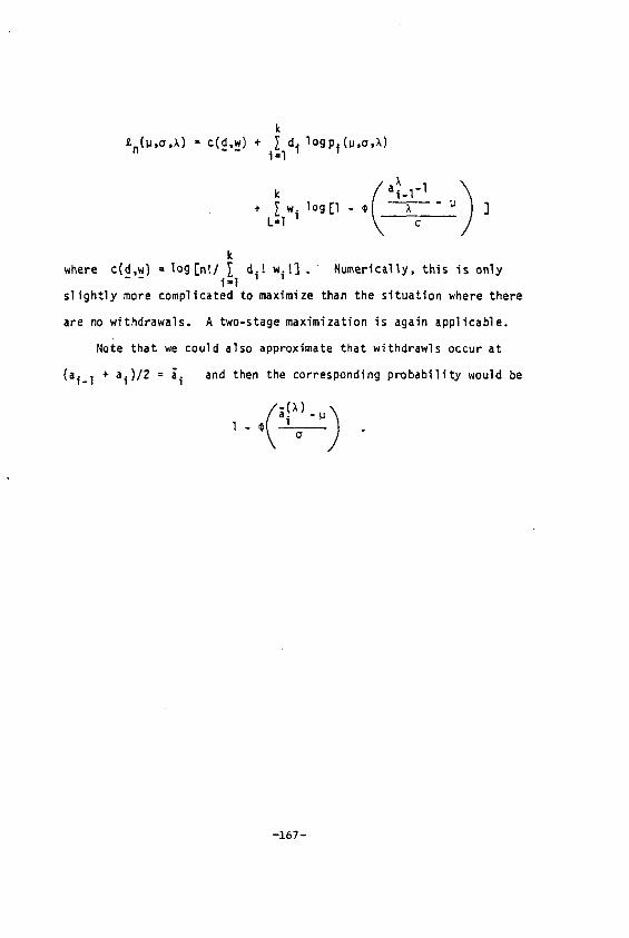
k ~n(~,a,~) - c(d,w) + iZldl logpi(~,a,X)

t!l,, i logrl ~ ~ ~

where c(d,w) ~ log[n!/ Z di! w i ! ] . Numerically, this is only l - I

slightly more complicated to maximize than the situation where there

are no withdrawals. A two-stage maximization is again applicable.

F(ote that we could also approximate that withdrawls occur at

(aid + ai)/2 = ai and then the corresponding probability would be

/i(x) -u 1 1-¢t i 7

-167-

. 0 4 0

. 0 3 5 "

, 030

. 0 2 5

. 0 2 0

.015

.OIO

.OOS

.000

Figure l

~ J J !

O.

Histogram and Inverted pdf in the Original Scale

r

2 0 , 4 0 • 6 0 • 8 0 . 1 O 0 . Age

-168-

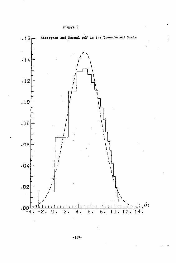
Figure 2

.16

.14

,12

.10

.08

.06

.04

.02

.00 - -L

E- L

L

Histogram and Normal pdf in the Transformed Scale

I I

I I

I I

I I

I I

f \

l l l l l I

I

I " I

i I

" l / I/ \ \ -,1 I , ~ , 1 i , l , l , l , ~ , l , l , l , l ' ~ l , l l , i " m . , . J ~ ( : ~ ' ) - • - 2 . O. 2. 4. 6. 8. IO. 12. 14.

-169-

BIBLIOGRAPHY

Abramowitz, M. and Stegun, I . A . (1964). Handbook of Mathematical Functions, Washington, D. C.: National Bureau of Standards, Applied Mathematics Series No. 55.

Benn, R. T. and Sidebottom, S. (1976). Algorithm AS-95: Maximum likelihood estimation of location and scale parameters from grouped data, A~pl. Statist.. 25, 88-93.

Box, G. E. P. and Cox, D. R. (1964). An analysis of transformations, J. R. Stat is t . Soc. B-26, 211-52.

Draper, N. R. and Cox, D. R. (1969). On distributions and their transformation to normality, J. Royal Stat ist . Soc. B~31., 472-76.

Hernafidez, A. F. and Johnson, R. A. (1981). Transformation of a discrete distr ibution to near normality, Stat ist ical Distributions in Scient i f ic Work 5, 259-270, C. Ta i l l i e et. al (eds.).

Kale, K. B. (1963). Some remarks on a method of maximum-likelihood estimation proposed by Richards, J. Royal Stat ist . Soc. B-25, 209-12.

Keyfitz, N. and Flieger, W. (1971). Population~ Facts and Methods of Demography. W. H. Freeman and Co.

Lindley, D. V. (1950). Grouping corrections and maximum likelihood equations, Proc. Camb. Philos. Soc. 46, I06-I0.

Richards, F. S. G. (1961). A method of maximum likelihood estimation, J. Royal Stat is t . Soc. B-23, 469-75.

Tukey, J.W. (1977), Explorqtory Data Analysis., Addison-Wesley, Reading, Mass.

-170-