Download pdf - ULTRACOLD QUANTUM MATTER IN LOWER DIMENSIONS

ULTRACOLD QUANTUM MATTER IN LOWERDIMENSIONS

A Dissertation

Presented to the Faculty of the Graduate School

of Cornell University

in Partial Fulfillment of the Requirements for the Degree of

Doctor of Philosophy

by

Stefan Baur

August 2011

c© 2011 Stefan Baur

ALL RIGHTS RESERVED

ULTRACOLD QUANTUM MATTER IN LOWER DIMENSIONS

Stefan Baur, Ph.D.

Cornell University 2011

Rapid progress in the field of ultracold atoms allows the study of many new and

old models of quantum many-body physics. In this doctoral dissertation we

theoretically explore exotic phases of ultracold quantum gases, with a special

focus spin-imbalanced attractive Fermi gases in lower dimensional situations.

Chapter 2 reviews the mean-field theory approach to pairing in two-

component Fermi gases. Applications of this theory are illustrated in Chapter

3, where we discuss mostly well-known results of mean-field theory applied to

imbalanced Fermi gases. Adapted from the author’s prior publications, Chap-

ters 4, 5 use the theory developed in Chapters 2, 3.

In Chapter 6 we discuss the physics of Fermi gases, squeezed into one spatial

dimension. In this and Chapter 7, we go beyond mean-field theory, approach-

ing the problem through the Bethe ansatz, exact solutions to few-body problems

and Fermi-Bose mappings (“fermionization”). We also show results from a joint

effort with the experimental group of Randy Hulet at Rice University to experi-

mentally realize and probe a strongly interacting one dimensional paired Fermi

gas.

In Chapter 8, after a brief introduction to rapidly rotating two dimensional

Bose gases, we introduce a new protocol to create few atom fractional quantum

Hall states.

Finally, in Chapter 9 we study the effects of two-body losses on lattice Bose

gases with hardcore interactions in one and two spatial dimensions.

BIOGRAPHICAL SKETCH

Stefan Baur was born in Heidelberg, Germany, on December 10, 1982 as the first

child of his father Klaus, a mechanical engineer, and his mother Marie-Luise, a

pharmacist and nutrition chemist.

Together with his younger brother Jörg, he grew up and went to high school

in Weinheim, Germany. After receiving his “Abitur” degree from the Werner-

Heisenberg-Gymnasium in Weinheim in 2002, he enrolled the same year at

the University of Heidelberg, Germany to study physics. After passing his

“Vordiplom” in 2004, he got a fellowship to spend the academic year 2005-2006

as an exchange student at Cornell University. After a very enjoyable year (with

an unusually mild winter) at the Cornell Physics department, he successfully

enrolled in the Physics Ph.D. program in 2006, where he joined the research

group of Prof. Erich Mueller at Cornell’s Lab of Atomic and Solid-State Physics.

During his Ph.D. studies he witnessed first hand the tremendous progress that

was happening in the field of ultracold gases. During this exciting time, he

worked on a variety of theoretical problems involving strongly correlated quan-

tum gases. After receiving his Ph.D., he will join the Theory of Condensed-

Matter group at the Cavendish Lab, University of Cambridge in the UK as a

post-doctoral researcher.

iii

To my parents

iv

ACKNOWLEDGEMENTS

First I would like to go back where it all started and thank my family. My par-

ents, Marie-Luise and Klaus, supported my interest in science from an early age.

Thanks for your encouragement, motivation and support! My first contact with

scientific research was when my uncle Gerhard let me spend a ten day intern-

ship in experimental nuclear physics at the Forschungszentrum Jülich while I

was still a high school student. Thanks for introducing me to the field I would

eventually pursue. Finally my brother Jörg, for being a companion through

childhood. Thanks for the fun times when we explored California and for let-

ting me crash at your place in Munich!

I probably had the best advisor I could possibly have had. Without Erich

Mueller this Ph.D. thesis would not have been possible. In our countless meet-

ings, I have many times seen him show brilliant insight on how to simplify

complicated problems. Most of my knowledge about physics, I have learned

from Erich.

I profited from lectures by many remarkable physicists, most notably Piet

Brouwer, Chris Henley, Jim Sethna and Dan Ralph. Thanks for being inspiring

physics teachers.

Much of the work leading to this thesis was done in my office in Clark Hall

and at various Collegetown coffee shops, where many afternoons were spent

talking physics (and not physics) with Stefan Natu and Kaden "Johnny" Haz-

zard. Thanks for being great friends, colleagues and gym buddies.

Thanks go to Mukund Vengalattore and Lauren Aycock for being the coolest

experimentalists. Thanks for repairing my laptop power supply and head-

phones in your cold atoms lab. In return I dragged you guys on Fridays for

beer at the Big Red Barn. Thanks for joining!

v

I would also like to thank my fellow graduate students, postdocs and friends

in the Cornell physics department. In particular (but no particular order): Sumi-

ran Pujari, Watson Chakram, Praveen Gowtham, Sufei Shi, Dominik Ho, Sour-

ish Basu, Ben Machta, Phil Kidd, Joern Kupferschmidt, Dan Goldbaum, Naresh

Kumar, Josh Berger, Johannes Lischner, Yoav Kallus, Alisa Blinova (physics

graduate student by association), Milan Allan, Sourish Basu, Steve Hicks, Mo-

hammed Hamidian, Darren Puigh, Ines Firmo, YJ Chen, Gang Xu, Dan Wohns,

Mark Fischer, Eliot Kapit and also all those I forgot to mention here.

I’m very grateful to Randy Hulet and his group at Rice, in particular Sophie

Rittner, Yean-an Liao, Tobias Paprotta and Ted Corcovilos for being great exper-

imental collaborators. I would never have learned nearly as much about cold

atom experiments without the great projects with you guys.

Thanks go also to the many theorists I collaborated with over the years: John

Shumway, Theja de Silva, Meera Parish and David Huse.

The organizers of the DARPA OLE meetings deserve a special acknowledge-

ment for hosting the best physics conferences in the best possible locations, such

as Las Vegas and Miami. The great atmosphere at these meetings will be missed.

I was fortunate to spend the summer of 2010 at a summer school in Les

Houches, France. This was a spectacular experience, and I would like to thank

Jildou Baarsma, Nir Navon, the nice weather, and many others for making this

a great time.

Beyond people in physics, it is almost impossible to thank everyone else. I

will try to mention a few others who greatly influenced my life in Ithaca.

I would like to thank the Cornell Field Hockey Club Team for providing me

with distraction from physics. In particular Jodi was a great friend for many

years in Ithaca. We enjoyed many Thursday nights playing darts after practice

vi

together with Marty and Chris at the Chapter House.

I should also thank my many house mates over the years for making my

rent affordable. Thanks to Johannes Heinonen, Hitesh Changlani, Leif Ristroph,

Ravishankar Sundararaman, Shivam Ghosh and Kshitij Auluck for sharing a

roof and being great friends.

Thanks to my girlfriend Natalia for everything and being patient whenever

I had to work on this thesis, and to our various friends among the Chapter

House/Big Red Barn regulars: Axel, Mary, Leifur and everyone else, whether

icelandic or not.

Finally, I would like to thank my friends from high school and college for

welcoming me back whenever I came home to Weinheim and Heidelberg!

Thanks to the US government for funding my research. This work was sup-

ported through ARO Award W911NF-07-1-0464 with funds from the DARPA

OLE Program and by the National Science Foundation through grant No. PHY-

0758104.

vii

TABLE OF CONTENTS

Biographical Sketch . . . . . . . . . . . . . . . . . . . . . . . . . . . . . . iiiDedication . . . . . . . . . . . . . . . . . . . . . . . . . . . . . . . . . . . ivAcknowledgements . . . . . . . . . . . . . . . . . . . . . . . . . . . . . . vTable of Contents . . . . . . . . . . . . . . . . . . . . . . . . . . . . . . . viiiList of Tables . . . . . . . . . . . . . . . . . . . . . . . . . . . . . . . . . . xiList of Figures . . . . . . . . . . . . . . . . . . . . . . . . . . . . . . . . . xii

1 Ultracold Bose and Fermi Gases 11.1 What are cold gases good for? . . . . . . . . . . . . . . . . . . . . . 11.2 Quantum gases . . . . . . . . . . . . . . . . . . . . . . . . . . . . . 21.3 Bose-Einstein condensation . . . . . . . . . . . . . . . . . . . . . . 41.4 Ultracold Fermi gases and Feshbach resonances . . . . . . . . . . 51.5 Appendix A: Effective models for scattering near a Feshbach res-

onance . . . . . . . . . . . . . . . . . . . . . . . . . . . . . . . . . . 8

Bibliography for Chapter 1 11

2 Mean-field theory for superfluid Fermi gases — Bogoliubov-deGennes equations 132.1 General setup . . . . . . . . . . . . . . . . . . . . . . . . . . . . . . 132.2 Mean-field approximation . . . . . . . . . . . . . . . . . . . . . . . 142.3 Variational principle . . . . . . . . . . . . . . . . . . . . . . . . . . 172.4 Gradient expansion . . . . . . . . . . . . . . . . . . . . . . . . . . . 192.5 Summary . . . . . . . . . . . . . . . . . . . . . . . . . . . . . . . . . 21


3 Applications of Bogoliubov-de Gennes theory to ultracold atoms 233.1 BEC-BCS crossover . . . . . . . . . . . . . . . . . . . . . . . . . . . 233.2 Effect of spin-imbalance — Clogston limit . . . . . . . . . . . . . . 283.3 Density profiles and phase diagrams . . . . . . . . . . . . . . . . . 333.4 Stability of the Fulde-Ferrell state in D = 3 . . . . . . . . . . . . . 363.5 Dark solitons and Andreev boundstates — A toy model for FFLO 403.6 Fulde-Ferrell versus Larkin-Ovchinnikov in 1D . . . . . . . . . . . 473.7 Appendix A: Asymptotic expansion for BCS and BEC limit . . . . 55

3.7.1 BCS limit . . . . . . . . . . . . . . . . . . . . . . . . . . . . . 553.7.2 BEC limit . . . . . . . . . . . . . . . . . . . . . . . . . . . . 57

3.8 Appendix B: Andreev boundstates for two domain walls . . . . . 59


viii

4 Deformed clouds of imbalanced fermionic superfluids 664.1 Abstract . . . . . . . . . . . . . . . . . . . . . . . . . . . . . . . . . 664.2 Introduction . . . . . . . . . . . . . . . . . . . . . . . . . . . . . . . 66

4.2.1 Background . . . . . . . . . . . . . . . . . . . . . . . . . . . 694.3 Calculation of Surface Tension . . . . . . . . . . . . . . . . . . . . . 74

4.3.1 Order of magnitude . . . . . . . . . . . . . . . . . . . . . . 754.3.2 Mean Field Theory . . . . . . . . . . . . . . . . . . . . . . . 754.3.3 Results (T = 0) . . . . . . . . . . . . . . . . . . . . . . . . . 804.3.4 Gradient expansion . . . . . . . . . . . . . . . . . . . . . . . 80

4.4 Effect of surface tension on density profiles . . . . . . . . . . . . . 834.4.1 Calculation of boundary . . . . . . . . . . . . . . . . . . . . 86

4.5 Summary and Conclusions . . . . . . . . . . . . . . . . . . . . . . 904.6 Acknowledgments . . . . . . . . . . . . . . . . . . . . . . . . . . . 924.7 Appendix A: Cutoff dependence of the BdG calculations . . . . . 924.8 Appendix B: Evaluation of phenomenological Free energy . . . . 93


5 Quasi-one-dimensional polarized Fermi superfluids 1025.1 Abstract . . . . . . . . . . . . . . . . . . . . . . . . . . . . . . . . . 1025.2 Introduction . . . . . . . . . . . . . . . . . . . . . . . . . . . . . . . 1025.3 Model . . . . . . . . . . . . . . . . . . . . . . . . . . . . . . . . . . . 1045.4 Phase diagram . . . . . . . . . . . . . . . . . . . . . . . . . . . . . . 1065.5 Experimental considerations . . . . . . . . . . . . . . . . . . . . . . 111


6 Theory and experiments with imbalanced Fermi gases in one dimen-sion 1166.1 Trapped Fermi gases in one dimension . . . . . . . . . . . . . . . . 1166.2 The spin imbalanced case . . . . . . . . . . . . . . . . . . . . . . . 1226.3 Extensions to finite temperature . . . . . . . . . . . . . . . . . . . . 1266.4 Correlations of the paired state . . . . . . . . . . . . . . . . . . . . 129

6.4.1 Simple strong coupling theory . . . . . . . . . . . . . . . . 1296.4.2 Predictions from weak coupling bosonization . . . . . . . 1346.4.3 Strong coupling bosonization . . . . . . . . . . . . . . . . . 139

6.5 Experimental probes of the 1D imbalanced Fermi gas . . . . . . . 1406.5.1 Experimental setup . . . . . . . . . . . . . . . . . . . . . . . 1406.5.2 Theory model . . . . . . . . . . . . . . . . . . . . . . . . . . 144

6.6 Appendix A: Truncation of TBA equations . . . . . . . . . . . . . 152


ix

7 FFLO vs Bose-Fermi mixture in polarized 1D Fermi gas on a Feshbachresonance: a 3-body study 1607.1 Abstract . . . . . . . . . . . . . . . . . . . . . . . . . . . . . . . . . 1607.2 Introduction . . . . . . . . . . . . . . . . . . . . . . . . . . . . . . . 1607.3 Qualitative Structure . . . . . . . . . . . . . . . . . . . . . . . . . . 1637.4 Wave functions . . . . . . . . . . . . . . . . . . . . . . . . . . . . . 1667.5 Quantum Monte Carlo (QMC) . . . . . . . . . . . . . . . . . . . . 1677.6 Realization/Detection . . . . . . . . . . . . . . . . . . . . . . . . . 1707.7 Acknowledgments . . . . . . . . . . . . . . . . . . . . . . . . . . . 1717.8 Appendix A: Solution of the 3-body problem . . . . . . . . . . . . 1717.9 Appendix B: Derivation of the path integral action and Monte

Carlo rules . . . . . . . . . . . . . . . . . . . . . . . . . . . . . . . . 173


8 Rotating Bose gases and fractional quantum Hall states 1788.1 Motivation — Rapidly rotating Bose gases . . . . . . . . . . . . . . 1788.2 Abstract . . . . . . . . . . . . . . . . . . . . . . . . . . . . . . . . . 1808.3 Introduction . . . . . . . . . . . . . . . . . . . . . . . . . . . . . . . 1818.4 Methods and Results . . . . . . . . . . . . . . . . . . . . . . . . . . 1838.5 Conclusion . . . . . . . . . . . . . . . . . . . . . . . . . . . . . . . . 190


9 Nonequilibrium effects of bosons in optical lattices 1949.1 Motivation . . . . . . . . . . . . . . . . . . . . . . . . . . . . . . . . 1949.2 Abstract . . . . . . . . . . . . . . . . . . . . . . . . . . . . . . . . . 1969.3 Introduction . . . . . . . . . . . . . . . . . . . . . . . . . . . . . . . 1969.4 Numerical Approach . . . . . . . . . . . . . . . . . . . . . . . . . . 1999.5 Time evolution of the density . . . . . . . . . . . . . . . . . . . . . 2019.6 Time evolution of two-site observables . . . . . . . . . . . . . . . . 2029.7 Entropy . . . . . . . . . . . . . . . . . . . . . . . . . . . . . . . . . . 2049.8 Induced losses as a probe of local spin correlations . . . . . . . . . 206

9.8.1 Two species fermions . . . . . . . . . . . . . . . . . . . . . . 2079.8.2 Two species bosons . . . . . . . . . . . . . . . . . . . . . . . 208


x

LIST OF TABLES

7.1 Gaussian sampling widths and Metropolis acceptance rule, A =min(1, e−∆STR/TF ), for moves in Figs. 7.3 (a)-(d). Moves for beadx′j → xj are sampled from a Gaussian of width σF centered aboutxj ; while the reverse moves xj → x′j sample a Gaussian of widthσR. . . . . . . . . . . . . . . . . . . . . . . . . . . . . . . . . . . . . 169

xi

LIST OF FIGURES

1.1 (a) shows the hyperfine structure of 6Li as a function of mag-netic field B. The lowest two hyperfine states are used in manyexperiments with ultracold Fermi gases. (b) Scattering lengthas as a function of magnetic field B for collisions between thetwo lowest hyperfine states |1〉 , |2〉 (using the parameterizationof Ref. [24]). Notable features are a broad Feshbach resonanceat B = 834 G (this is where most experiments are performed).Other features special to 6Li are the zero crossing around 500 Gand the large negative scattering length at high fields (i.e. thedeep BCS limit is inaccessible). . . . . . . . . . . . . . . . . . . . . 7

3.1 Variation of order parameter ∆ (a) and chemical potential µ (b)as a function of 1/(kFas) from BCS to BEC limit, calculated frommean-field theory. The dashed line in (a) is the BCS limit resultfor the energy gap ∆ ∼ 8e−2eπ/(2kF as). In (b) we have also plotted1/2 of the two-body bound-state energy εB = −~2/(ma2

s) for as >0 (dashed line). . . . . . . . . . . . . . . . . . . . . . . . . . . . . . 25

3.2 Mean-field Bogoliubov excitation spectrum in the BCS (a) andBEC (b) limit (solid lines). Note how the character of thefermionic excitations depends on the sign of µ = 0. The dashedlines are the corresponding noninteracting spectra with ∆0 = 0. . 27

3.3 Global topology of the mean-field theory phase diagram of thepolarized Fermi-gas at T = 0 [44, 45, 46, 47, 48, 49, 50, 51, 52].We plot the phase-diagram in the units of Ref. [50], where wepractically work at fixed h, µ and normalize h with the energygap Egap from Eq. (3.11). Note that we define kF with referenceto the density of the h = 0 superfluid. Many qualitative fea-tures of this mean-field phase diagram are believed to be correctand have mostly been confirmed in experiments [53, 54, 55]. In-cluding interactions in the normal state shifts the transition linebetween partially and fully polarized normal to the right (recentQMC calculations suggest that the line is even shifted beyondthe critical point where the Bose-Fermi mixture becomes a stablephase [51]). In brackets we indicate whether a phase is polarized[P = (n↑ − n↓)/(n↑ + n↓)]. . . . . . . . . . . . . . . . . . . . . . . . 31

3.4 Phase diagram of a Bose-Fermi mixture, calculated from theHartree-Fock free energy Eq. (3.23). The values of the boson-fermion scattering length are aBF = 1.2as and aBB = 0.6as (theseparameters differ from the mean-field results and are appropri-ate for the imbalanced Fermi gas in the BEC limit) [58, 59, 10].The boson (fermion) chemical potentials µB (µF ) are normalizedby half the binding energy εB/2 = ~2/(2ma2

s) of the pairs. . . . . 34

xii

3.5 Mean-field phase diagram of the imbalanced Fermi gas in theBCS limit (in 3D). There is a tiny sliver of stable FFLO phase,sandwiched between the dashed and solid line. This FFLO phaseappears to be stable up to (h/εB, µ/εB) ≈ (0.42, 1.39) (FFLO isstable for (kFas)

−1 ≤ −0.56). The solid (dashed) line representsa first order first (second) order phase transition respectively. . . 37

3.6 (a) Mean-field free energy as a function of the superfluid orderparameter δ = ∆/∆0 for a series of Zeeman magnetic fieldsh/hc = 0, 0.5, 0.8, 1.0 at kFas = −1. Note that at the Clogstonlimit h = hc there appears to be a first order phase transition tothe normal state when the minima in the free energy are degener-ate. (b) Minimum of the kernelK(2)(qmax) (related to the pair sus-ceptibility) as a function of interaction strength on the Clogstonlimit. The normal state becomes unstable towards FFLO around(kFas)

−1 ≤ −0.56. (c) K(2)(q) plotted at fixed interaction strength(kFas)

−1 = −1 at, above and below the Clogston limit. (In all fig-ures we have defined kF always via the unpolarized superfluidstate at h = 0) . . . . . . . . . . . . . . . . . . . . . . . . . . . . . . 38

3.7 Top: Andreev boundstate wavefunctions (u(z), v(z))T for pa-rameters in the BCS regime (in terms of the dimensionless unitsdescribed in the text, we used ∆0 = 1, µ = 5, d = 20). (a)Positive energy bound-state solution for a single domain wall∆(z) = sign(z)∆0. (b) Symmetric solutions for two domain walls∆(z) = ∆0 (sign(d/2 + z)− sign(z − d/2)− 1). Bottom: (c) Toymodel for low polarization density FFLO: An array of weaklyinteracting sharp domain walls. The boundstates, localized ateach domain wall, start to overlap and give rise to a bandstruc-ture. (d) Bound state energies for the configuration of two do-main walls in (b), where the distance d between the kinks is varied. 41

3.8 Dispersion relation of the Andreev boundstate of a π-domainwall in 2D or 3D (units have ~2/(2m) = 1). The dashed linerepresents the gap to Bogoliubov quasiparticle excitations, Egap. . 46

xiii

3.9 Top: (a) Mean-field theory phase diagram of a 1D Fermi gas in-teracting with attractive interactions with scattering length a (weneglected Hartree shifts). On the black line a π-domain wallhas the same energy as the uniform superfluid, indicating aninstability of the P=0 superfluid towards FFLO. The red line isthe first order phase boundary between superfluid and FF stateand the dashed line is the Clogston limit. (b) Free energy ofthe FF state as a function of ∆0, q [see Eq. (3.61)] for (h, µ) =(0.56, 1.13)~2/(ma2). Local minima are marked with a red dot.Bottom: (c) Dispersion relation of Bogoliubov quasiparticles forthe FF state ansatz ∆(z) = ∆0e

iqz shown here for the parametersof (b). (d) Self-consistent solutions to the 1D BdG equations fordifferent polarization densities at fixed µ = 2.25~2/(ma2). In thelimit of low polarization density, the FFLO phase consists of sep-arated domain walls and the order parameter achieves the valueof the uniform superfluid in between nodes. At large polariza-tion the magnitude of the order parameter reduces and ∆(z) be-comes sinusiodal. In this limit ∆(z) closely resembles the LO state. 48

3.10 Self-consistent solution to the BdG equations in 1D for a har-monically trapped system with N↑ = 70, N↓ = 66, µ(z = 0) =2.25~2/(ma2). Left: ∆(z) with and without imbalance. Each nodein the order parameter corresponds to one excess fermion. Right:Density of up-spins n↑(z) (down-spins n↓(z)) respectively. Notethat at low polarization the density profile in 1D is inverted withrespect to the 3D scenario. The fully paired phase sits on theinside, whereas the FFLO is visible at the trap center. . . . . . . . 54

4.1 Schematic phase diagram of a two component Fermi gas asa function of (a) Temperature [T ] - Polarization [P = (n↑ −n↓)/(n↑+n↓)], (b) Temperature [T ] - chemical potential difference[h = (µ↑ − µ↓)/2], and (c) chemical potential [µ = (µ↑ − µ↓)/2]- chemical potential difference [h = (µ↑ − µ↓)/2]. The equationof state sets a relationship between P, T, h, and µ, so only threeof them are needed to specify the state. Solid lines: continuousphase transitions; dashed lines: discontinuous; these meet at thetricritical point [Pt, ht, Tt] or [µt, ht, Tt]. The gray region in (a)maps onto the dashed line in (b), and represents a coexistenceregion. On the BCS side of resonance a < 0, and for sufficientlylarge a, P1=0 and 0 < P2 < 1. When a > 0 decreases in magni-tude, P1 and P2 move to the right, sequentially hitting the maxi-mum allowed value P = 1. At unitarity, a =∞, a Wilsonian RGtheory[59] predicts Pt = 0.24 and Tt/TF,↑ = 0.06. Monte-Carlocalculations suggest Tc/TF = 0.152(7)[60], and P2 = 0.39[58]. . . 72

xiv

4.2 Order parameter profiles at the interface between normal and su-perfluid at critical Zeeman field hc. Left to right: BCS to BEC sideof resonance. Each data point corresponds to a single gridpointof our real space discretization. Insets: normal state T -matrix(pair susceptibility) as a function of momentum q at the first or-der phase transition line h = hc corresponding to the same pa-rameters as the BdG calculations. The Fourier transform of T (q)describes the decay of the superfluid order parameter into thepolarized normal state. The vertical line shows q = k↑F − k↓F . . . . 76

4.3 Dimensionless surface tension η = 2~−2mn−4/3s σ as a function

of (kFa)−1 at T = 0. When (kFa)−1 > 1.01 the superfluid stateis partially polarized. Triangles: calculation using the full BdGequations as described in 4.3.3, circles: gradient expansion ap-proximation to this solution from 4.3.4. The lines are a guide tothe eye. . . . . . . . . . . . . . . . . . . . . . . . . . . . . . . . . . 81

4.4 Experimental two-dimensional column densities (black denoteshigh density) for P = 0.38 with theoretically calculated bound-aries for different surface tensions η (fixing the number of parti-cles to be constant). Top: majority atoms N↑; Bottom: minorityatoms N↓. The dotted line is the ellipse with semi-major andsemi-minor axes ZTF and RTF respectively, while the solid line isthe superfluid-normal boundary in the presence of surface ten-sion. As η is increased, the superfluid-normal boundary deformsfrom an elliptical iso-potential surface, but the boundary be-comes increasingly insensitive to surface tension with increasingη. Nc = 15 Fourier components were chosen for equation (4.24).Data corresponds to Fig. 1(c) in Ref. [2], used with permission.Data outside of an elliptical aperture has been excluded. Thistruncation of the data leads to a slight discrepancy in P com-pared to the value quoted in [2]. Each panel is 1.4mm×0.06mm,and shows the true aspect ratio of the cloud. . . . . . . . . . . . . 84

4.5 Axial densities. Symbols: experimental one-dimensional 6Lispin densities and density differences for P = 0.39 (N↑ =155, 000, N↓ = 68, 500) (left column) and P = 0.63 (N↑ =123, 600, N↓ = 28, 000) (right column), from Ref. [2], with permis-sion. Lines: theoretical curves for η = 2.83, taking a cigar shapedharmonic trap with small oscillation frequencies ωz = (2π)7.2Hzand ωr = (2π)325 Hz. Oscillations in the density differencewithin the superfluid region are artifacts of our ansatz (4.24).To minimize noise, only experimental data inside an ellipticalwindow was considered (see text). This aperture is visible in fig-ure 4.4. . . . . . . . . . . . . . . . . . . . . . . . . . . . . . . . . . 85

xv

4.6 Distortion of superfluid core aspect ratio (= 1 − F (π/2)/F (0))in % as a function of the dimensionless surface tension η for pa-rameters of Ref [5], where λ is the aspect ratio of the harmonictrap. . . . . . . . . . . . . . . . . . . . . . . . . . . . . . . . . . . . 89

4.7 Top: Representative order parameter profiles for different cut-offs computed using the BdG equations at 1/kFa = 0.05. Forbetter visibility a line connecting the data points is displayed.Bottom: Dimensionless surface tension constant η for differentcutoffs as a function of 1/kFa. . . . . . . . . . . . . . . . . . . . . . 94

5.1 (Color online) Phase diagram for h = 0. For t/εB below thefilled circle, there is a two-atom bound state, and the resultingbosonic pairs enter the system as a Bose condensate as µ is in-creased through the solid line. For t/εB above the filled circle weare always in the BCS regime. . . . . . . . . . . . . . . . . . . . . 107

5.2 (Color online) Slice of the mean-field phase diagram taken att/εB = 0.08. The phases shown include the unpolarized super-fluid (SF), partially-polarized normal (N), and fully-polarizednormal (NP). The FFLO phase is divided into gapped ‘commen-surate’ (C) and ungapped ‘incommensurate’ (IC) phases. Thefilled circle marks the tricritical point; near it, but not visible hereis a tiny region of SFM phase, a remnant of the 3D BEC regime.The SF-NP and SF-N transitions are first-order for µ/εB abovethe tricritical point, along the solid heavy line. The SF-FFLOtransition (solid line) is estimated from the domain wall calcu-lation. The transition from FFLO to normal (dotted-dashed line)is assumed to be second-order. The large circle marks the regionof FFLO where ∆/εF is largest, so the phase is likely most ro-bust to T > 0 here. The dashed line near the SF-FFLO transitionshows where the wave vector of the FFLO state is stationary as afunction of µ: dq/dµ = 0 (this is calculated using the FF approxi-mation). . . . . . . . . . . . . . . . . . . . . . . . . . . . . . . . . . 109

6.1 Phase diagram of the 1D attractive Fermi gas Eq. (3.56) as calcu-lated from a solution to the Bethe ansatz integral equations (6.20)(chemical potentials are scaled by the two-body binding energyεB = ~2/(ma2

1D)). The SF region is an unpolarized (n↑ = n↓)and fully paired phase. The 1D FFLO phase has n↑ > n↓ > 0,featuring spatially modulated superfluid correlations. At largeZeeman field h the gas becomes fully polarized, here labeled FP.The arrows correspond to the ranges of µ, h of the (trapped sys-tem) density profiles shown in Fig. 6.2. Note that for a trappedimbalanced gas, three distinct phase sequences are possible [(a)→ FFLO/SF, (b)→ FFLO, (c)→ FFLO/FP], as shown in Fig. 6.2. 125

xvi

6.2 Density profiles at zero (dashed lines) and finite temperatureT/εB = 0.03 (solid lines) for a 1D imbalanced Fermi gas in aharmonic trap. The red curves show the total density na1D andthe blue curves the density difference (n↑ − n↓)a1D. The densi-ties were calculated from a solution to the Bethe ansatz integralequations and using local density approximation. The centralchemical potential is the same for all plots (µcentral/εB = −0.3).Position z along the tubes is scaled by the factor a2

z/a1D, whereaz is the harmonic oscillator of the harmonic trapping potential.Note that in the moderate imbalanced regime shown in (c), thedensity difference in the FFLO phase varies only by a few per-cent, thus making a detection of FFLO feasible even in an inho-mogeneous trap. . . . . . . . . . . . . . . . . . . . . . . . . . . . . 126

6.3 An in-trap version of the (T = 0) phase diagram Fig. 6.1, wherewe show the more easily experimentally accessible quantitiesof minority (red) and majority (blue) Thomas-Fermi radii for aharmonically trap gas (see [1, 22]). The radii are normalizedby az

√N , where az is the 1D harmonic oscillator length for the

trapping potential. Note that the minority- and majority-radiuscross around 15% polarization (when the edge of the cloud hitsthe multicritical point). When plotted in these variables, thephase diagram is not universal anymore in the sense that it stillhas a (weak) dependence on the ratio between Fermi energyand binding energy κ = (~ωN/2)/εB = Na2

1D/a2z [1]. Here the

plot is shown for typical parameters of the Rice experiments,κ = Na2

1D/a2z ≈ 0.26 (where N ≈ 170, a1D = 0.11µm, az = 2.83µm). 127

6.4 Strong coupling limit of Gaudin-Yang model: Here we sketch therelative wavefunction between pairs (bosons) (a) and a pair andexcess fermion (b) in the strong coupling/low density limit as afunction of the relative coordinate x in a fictitious box of length Lwith the boundary condition that the derivative vanishes at x =±L/2. The interaction between bosons becomes hardcore at lowdensity. What is remarkable is that the pair-fermion interactionvanishes apart from a phase shift of π. . . . . . . . . . . . . . . . . 131

6.5 Long distance properties of CF (R) (shown in (a) for filling νF =πnfa = 0.1 and the hardcore Bose correlation function CB(R) forνB = 0.2 (b), both shown as a function of lattice site index i = Ron a log-log plot(solid blue lines). The dashed lines are fits to theasymptotic expressions, Eqs. (6.29) for (a)[(6.30) for (b)]. . . . . . 133

xvii

6.6 (a) Bose correlation function C(R) calculated from the mappingon non-interacting fermions described in the text (here shown forfillings νB = 0.2, νF = 0.1). (b), (c): Fourier transforms of C(R)(time-of-flight momentum distributions) for two different fillingfactors. The peaks at the FFLO pairing vector kF = πνF havea log-singularity (this is because we are in the strong couplinglimit. For weaker interactions one would see a cusp singularity).In (c) the dashed curve shows the effect of finite temperature.Here T/t = 0.1, where t is the boson/fermion hopping (that wearbitrarily took to be the same). . . . . . . . . . . . . . . . . . . . . 135

6.7 (a) Illustration of the crossed beam trap in the Rice experiment. Itcreates a harmonic potential plus a tight 2D lattice for the atomiccloud, confining the atoms to 1D tubes. (b) Perpendicular to the1D tubes, the potential is a superposition between a harmonictrap and a lattice potential of the form V0 sin2(kz), where k =2π/λ, λ = 1064 nm is the laser wavelength. . . . . . . . . . . . . . 141

6.8 (a),(b): Scattering length and binding energy for atoms con-fined to 1D as a function of the ratio between s-wave scatter-ing length as and harmonic oscillator length a⊥ of the transverseconfinement (from Ref. [11, 13]). In (b) the dashed lines showhow the binding energy approaches the value of the binding en-ergy of a 1D contact interaction in the BCS limit [with scatter-ing length from (a)] and how EB approaches the molecular limit~2/(ma2)− ~ω⊥. (c), (d) show results for the specific parametersof the two lowest hyperfine states of 6-Li and the lattice of theRice experiment (V0/ER = 12). The experiment of Ref. [22] wasperformed at 890 Gauss (indicated by the dashed vertical line)near the Feshbach resonance at 835 Gauss, which is is well onthe BCS side of the 1D confinement induced resonance. . . . . . . 146

6.9 (a), (b) show experimental column densities from the Rice group.(a) shows an unpolarized data set, where all atoms are expectedto be paired. The observed aspect ratio of ∼ 2 is different fromthe Thomas-Fermi expectation of 3. We attribute this differenceto a radial density distribution that froze in at some point whilethe atoms were loaded into the 2D lattice. (b) shows a columndensity of spin-up atoms at high polarization P ≈ 0.8. The un-bound free atoms have a higher tunneling rate than the pairs andappear to equilibrate on experimental time scales. . . . . . . . . . 147

6.10 Here we illustrate how we can still extract the distribution of par-ticle numbers from column density profiles using the an inverseAbel transformation. We sum up the rows of the density profilesto obtain the axial profile. This axial profile is then modeled us-ing a simple functional form and inverse Abel transformed to inorder to obtain N2(ρ) ≡ N↓(ρ) . . . . . . . . . . . . . . . . . . . . . 150

xviii

6.11 Thomas-Fermi radii of the central tube, extracted from an ensem-ble of experimental data sets for the 1D attractive imbalancedFermi gas (dots). Each radius is scaled by the factor az

√N and

the polarization refers to the central tube (N , P are found viaan inverse Abel transform). The solid lines are theory curvescorresponding to T = 0, 175, 200nK (where the T = 175nK curvewas the best fit obtained through interpolation). The theory radiiwere obtained from column density profiles with the same ex-traction method as the experimental ones. . . . . . . . . . . . . . 152

6.12 Sample dressed energies ε(k), κ(k) at T = 0.01 (c′ = −0.5) andµ = h = 0 (for these parameters, the gas is practically unpolar-ized, so ρ(k) ≈ 0). The gap in κ(k) is basically equal to the spingap ∆s. . . . . . . . . . . . . . . . . . . . . . . . . . . . . . . . . . . 156

7.1 (Color online) Cartoon depictions of the physics of Eq. (7.1) inthe BEC (left) and BCS (right) limits. (Top) Symmetry of Bosewave function: in the BCS limit the wave function changes signwhenever a pair passes a (spin-up) fermion. (Middle) Depictionof lattice model which is used for developing intuition about Eq.(1). (Bottom) Typical world lines illustrating interaction of a bo-son (heavy line) and fermion (thin line) with space along the hor-izontal axis and imaginary-time along the vertical axis. . . . . . 164

7.2 (Color online) The dimensionless 1D scattering lengths as/a =as/ag

2/3 for the symmetric (solid red line)/antisymmetric(dashed blue line) channel plotted vs the dimensionless de-tuning ν = ν/g4/3. The dotted (dashed dotted) line is theasymptotic result for as, as = 3ν/g2 (as = (3/2)ν/g2) in theBCS limit (BEC limit); (cf [10]). (Inset) Sum as + aa (solidline) crosses zero at ν ≈ −0.635, marking the change in sym-metry of the ground state. (c)-(e) Lowest-energy symmetric(solid line)/antisymmetric (dashed line) wave function fs/a(x) =L−1/2

∑Q e

iQxfs/a,Q, in a hard-wall box of size L ≈ 160/g2/3,where x represents the relative separation of the boson andfermion. Left to right: ν = −1,−0.635, 1. (f)-(h) Wave func-tion near the origin. Finite range of the effective interaction isapparent from the nonsinusoidal shape of f for small x. (i)-(k) Reduced density-matrix ρ(x, x′) defined in the text beforeEq. (7.6) for β = 100/g4/3 calculated with QMC. Blue/red rep-resents positive/negative weight. Quadrants with predominantpositive/negative weight are labeled with “+”/“–”. . . . . . . . 165

xix

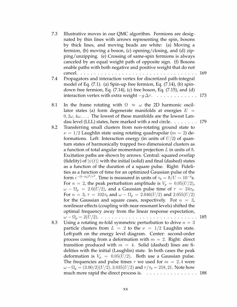
7.3 Illustrative moves in our QMC algorithm. Fermions are desig-nated by thin lines with arrows representing the spin, bosonsby thick lines, and moving beads are white: (a) Moving afermion, (b) moving a boson, (c) opening/closing, and (d) zip-ping/unzipping. (e) Crossing of same-spin fermions is alwayscanceled by an equal weight path of opposite sign. (f) Bosonsenable paths with both negative and positive weight that do notcancel. . . . . . . . . . . . . . . . . . . . . . . . . . . . . . . . . . . 169

7.4 Propagators and interaction vertex for discretized path-integralmodel of Eq. (7.1). (a) Spin-up free fermion, Eq. (7.14), (b) spin-down free fermion, Eq. (7.14), (c) free boson, Eq. (7.15), and (d)interaction vertex with extra weight −g∆τ . . . . . . . . . . . . . 173

8.1 In the frame rotating with Ω ≈ ω the 2D harmonic oscil-lator states (a) form degenerate manifolds at energies E =0, 2ω, 4ω, . . .. The lowest of these manifolds are the lowest Lan-dau level (LLL) states, here marked with a red circle. . . . . . . . 179

8.2 Transferring small clusters from non-rotating ground state toν = 1/2 Laughlin state using rotating quadrupolar (m = 2) de-formations. Left: Interaction energy (in units of U/2) of quan-tum states of harmonically trapped two dimensional clusters asa function of total angular momentum projection L in units of ~.Excitation paths are shown by arrows. Central: squared overlap(fidelity) of |ψ(t)〉with the initial (solid) and final (dashed) statesas a function of the duration of a square pulse. Right: Fideli-ties as a function of time for an optimized Gaussian pulse of theform e−(t−t0)2/τ2 . Time is measured in units of τ0 = ~/U ∼ 10−4s.For n = 2, the peak perturbation amplitude is Vp = 0.05(U/2),ω − Ωp = 2.0(U/2), and a Gaussian pulse time of τ = 24τ0.For n = 3, τ = 102τ0 and ω − Ωp = 2.046(U/2) and 2.055(U/2)for the Gaussian and square cases, respectively. For n = 3,nonlinear effects (coupling with near-resonant levels) shifted theoptimal frequency away from the linear response expectation,ω − Ωp = 2(U/2). . . . . . . . . . . . . . . . . . . . . . . . . . . . . 185

8.3 Using a rotating m-fold symmetric perturbation to drive n = 3particle clusters from L = 2 to the ν = 1/2 Laughlin state.Left:path on the energy level diagram. Center: second-orderprocess coming from a deformation with m = 2. Right: directtransition produced with m = 4. Solid (dashed) lines are fi-delities with the initial (Laughlin) state. In both cases the peakdeformation is Vp = 0.05(U/2). Both use a Gaussian pulse.The frequencies and pulse times τ we used for m = 2, 4 wereω−Ωp = (3.00/2)(U/2), 3.035(U/2) and τ/τ0 = 218, 21. Note howmuch more rapid the direct process is. . . . . . . . . . . . . . . . 188

xx

8.4 Transfering atoms using multiple pulses. Left: paths from ini-tial to Laughlin states for n = 3, 4. Right: Solid line is the fi-delity with the initial state, dotted with the intermediate (L,E) =(2~, 3(U/2)) state, and the dashed line with the Laughlin state.All pulses are Gaussians. Despite using multiple pulses, thistechnique is faster than using a higher order m = 2 pulse. Thefrequencies (Ωp), shape (m), and pulse times (τ ) for the N = 3sequence were ~(ω − Ωp)/(U/2) = 3.00, 3.035, m = 2, 4, andτ/τ0 = 16.95, 19.2. For both, Vp = 0.05(U/2). For N = 4, us-ing two pulses with m = 2 and Vp = 0.2(U/2), we achieve > 98%fidelity after a total two-pulse sequences with ~(ω−Ωp)/(U/2) =3.130, 1.0376 and τ/τ0 = 82.5, 87.0. . . . . . . . . . . . . . . . . . . 189

9.1 Left: Average particle number 〈N〉 =∑

n nTr ρ(n) as a func-tion of time for an initial Mott insulator state on a L = 10 lat-tice. Solid line: numerical simulation; Dotted line: two-bodydecay law for an uncorrelated state N(t) = N(0)/(1 + 2Γt). Mid-dle: Same, but for a Tonks-Girardeau gas initial state (groundstate of a hard core lattice gas with L = 10, N = 6). Solidline: simulation. Green dashed curve: two-body decay lawfor an uncorrelated state. N(t) = N(0)/(1 + 2Γt), Dotted line:two-body decay low assuming time independent correlationsN(t) = N(0)/(1 + 2g(2)(0)n(0)Γt). Right: Average particle num-bers in the different sectors 〈N (n)(t)〉 = nTr ρ(n)(t) for the Mottinsulator initial state. The sum of all curves at a certain timegives the blue in the leftmost figure. All times measured in unitsof the inverse hopping J−1. . . . . . . . . . . . . . . . . . . . . . . 195

9.2 Time evolution of correlation functions starting from (left) the 10particle Mott Insulator (L = 10, N = 10) or (right) the 6 parti-cle Tonks-Girardeau state (L = 10, N = 6). Thick line: t = 0;Dashed line: t = 200J−1; Thin lines: intermediate times sep-arated by 20J−1; Dotted line: The single particle density ma-trix 〈a†iai+j〉 one would expect if each of the n-particle sectorswere in their ground state at t = 200J−1. The insets of thelower-left and lower-right figures show g(2) as a function of den-sity n = N/L together with the analytic formula for an infinitehardcore boson system in the ground state at the same densityg

(2)eq (n) = 1− [sin(πn)/(nπ)]2. . . . . . . . . . . . . . . . . . . . . . 200

xxi

9.3 Left: Entropy S as a function of average particle number 〈N〉during time evolution, starting from the (top, solid line) L =12, N = 12 Mott insulator, (top, dashed-dotted line) 4×3, N = 12(2D) Mott insulator and (bottom, solid line) L = 12, N = 6Tonks-Girardeau initial states. Dashed line: analytic formulaS ∼ ln

(N(0)N

). Right: Entropy per particle as a function of time

starting from the (solid line) L = 12, N = 12 Mott Insulatorand (dashed line) L = 12, N = 6 Tonks-Girardeau state withΓ = 0.01J . . . . . . . . . . . . . . . . . . . . . . . . . . . . . . . . . 204

xxii

LIST OF PUBLICATIONS

1. Meera M. Parish, Stefan K. Baur, Erich J. Mueller, David A. Huse, Quasi-

one-dimensional polarized Fermi superfluids, Physical Review Letters 99,

250403 (2007).

2. Stefan K. Baur, Kaden R. A. Hazzard, Erich J. Mueller, Stirring trapped

atoms into fractional quantum Hall puddles, Physical Review A 78, 061608

(R) (2008).

3. Stefan K. Baur, Sourish Basu, Theja N. De Silva, Erich J. Mueller, Theory of

the Normal/Superfluid interface in population imbalanced Fermi gases, Physical

Review A 79, 013415 (2009).

4. T. A. Corcovilos, Stefan K. Baur, J. M. Hitchcock, E. J. Mueller, R. G. Hulet,

Detecting antiferromagnetism of atoms in an optical lattice via optical Bragg scat-

tering, Physical Review A 81, 013415 (2010).

5. Stefan K. Baur, John Shumway, Erich J. Mueller, FFLO vs Bose-Fermi mixture

in polarized 1D Fermi gas on a Feshbach resonance: a 3-body study, Physical

Review A 81, 033628 (2010).

6. Yean-an Liao, Ann Sophie C. Rittner, Tobias Paprotta, Wenhui Li, Guthrie

B. Partridge, Randall G. Hulet, Stefan K. Baur, Erich J. Mueller, Spin-

Imbalance in a One-Dimensional Fermi Gas, Nature 467, 567 (2010).

7. Stefan K. Baur, Erich J. Mueller, Two-body recombination in a quantum me-

chanical lattice gas: Entropy generation and probing of magnetic short-range

correlations, Physical Review A 82, 023626 (2010).

xxiii

CHAPTER 1

ULTRACOLD BOSE AND FERMI GASES

1.1 What are cold gases good for?

Since the creation of the first Bose-Einstein condensate (BEC), the field of ultra-

cold gases has tremendously enhanced our understanding of quantum many-

body physics [1, 2, 3, 4]. One can say that the field is now evolving into

what might be called quantum engineering. Toy models, introduced as sim-

plifications of complicated solid state systems that contain only the basic, but

non-trivial, physics, are now routinely created in atomic physics labs. These

cold quantum gases show an unprecedented degree of tunability and control

through the interplay of slow motion combined with the high degree of control

of quantum optics [5, 6, 7]. While cold gases in the laboratory naturally interact

very little with their environment, we often cannot directly harvest the remark-

able properties of these systems. Apart from using cold atoms as sensors, their

main applications will probably lie in the combination of quantum mechanics

and information processing. An early application of this sort was an experiment

by Lene Hau at Harvard, where a beam of light was slowed down to a few me-

ters per second, basically stored in a BEC [8]. More recently, cold gases are start-

ing to be used as a tool to simulate simple quantum many-body theories [9, 10].

Certain materials found in nature display quite unusual and puzzling proper-

ties. One of these systems are the high temperature (high-Tc) superconductors,

whose strongly correlated nature inhibits our understanding. While theorists

have found simple models (called model Hamiltonians) that should capture the

basic physics of high-Tc superconductors, these models are still far from fully

1

understood. The reason for this lack of understanding lies in the enormous size

of the possible quantum states (Hilbert space) of a quantum system of even few

particles and the general difficulty of simulating fermionic particles (like elec-

trons) on a computer. A quantum simulator would be a physical system repre-

senting a given model HamiltonianH , that would allows for its simulation and,

through various probes, would pave the way to understand its physics [11].

For new real complex materials, we envision that once we have made a list of

basic candidate Hamiltonians, cold atom quantum simulators will allow us to

map out their properties (phases of matter), bypassing the complexity of the

original problem. That way a quantum simulator allows us to gain information

about nature that was previously inaccessible (when working with hardware

governed by classical mechanics).

If we can control quantum mechanical particles and phases at will, this opens

up new potential applications. The creation of topologically ordered states, ei-

ther as analogs of fractional quantum hall states or novel forms of superconduc-

tivity, is within reach [12, 13, 14]. Bold proposals to build quantum computers

with cold neutral gases do not seem completely impossible anymore [15]. In the

long run, quantum information might be the field where ultracold gases will

have the most impact.

1.2 Quantum gases

When dilute atomic gases are cooled to ultra-low temperatures, quantum me-

chanics starts to become important. We can heuristically understand this be-

havior from simple dimensional analysis. A non-interacting classical gas is de-

2

scribed by a single length-scale, namely the inter-particle spacing l ∼ n−1/3,

where n is the density of a three-dimensional gas. The classical gas must there-

fore be scale invariant, without any phase transition as the temperature is low-

ered. Because of their attractive interactions, most gases that we know from ev-

eryday life undergo phase transitions to liquid and solid phases at sufficiently

low temperatures. This happens when the characteristic energy scale of the

ideal gas, kBT , becomes comparable to their interaction energy Eint. In dilute

gases, interactions are less important and these systems remain gaseous down

to very low temperatures. However, quantum mechanics provides us with a

new fundamental constant: Planck’s constant h. In addition to the inter-particle

spacing, there appears another length-scale (thermal de Broglie wavelength)

λT ∼h√

mkBT. (1.1)

We anticipate quantum mechanics to be important when inter-particle spacing

and the de Broglie length become comparable, i.e. when

kBT ∼h2

ml2∼ ~2n2/3

m. (1.2)

A surprising consequence of quantum mechanics is that identical particles that

technically to do not interact feel each other’s presence when their wavefunc-

tions overlap. The quantum mechanical wavefunction for two identical par-

ticles ψ(r1, r2) must have the same magnitude (probability density) when the

coordinates of the particles are exchanged

ψ(r1, r2) = eiφψ(r2, r1) (1.3)

When we repeat the exchange we expect to get our original wavefunction back,

therefore usually one has either φ = 0 or φ = π for bosons or fermions. The

ground state of a non-interacting Bose gas of N particles is the state where all

3

particles occupy the lowest energy single particle orbital

ψB(r1, . . . , rN) = φ1(r1) . . . φ1(rN) (1.4)

whereas the ground state of N (spinless) fermions is

ψF (r1, . . . , rN) =1√N !

∣∣∣∣∣∣∣∣∣∣∣∣∣

φ1(r1) φ1(r2) . . . φ1(rN)

φ2(r1) φ2(r2) . . . φ2(rN)

...... . . . ...

φN(r1) φN(r2) . . . φN(rN)

∣∣∣∣∣∣∣∣∣∣∣∣∣(1.5)

where the single particle orbitals φi(r) are chosen such that their energies εi are

the lowest N single particle energies.

1.3 Bose-Einstein condensation

The ground state Eq. (1.4) is a pure Bose-Einstein condensate, where all particles

occupy the lowest single particle eigenstate. At finite temperature T ≡ (kBβ)−1,

one finds that the total particle number of a non-interacting Bose gas is given by

N =∑i

ni (1.6)

where the average occupation number ni of orbital i are given by Bose-Einstein

statistics

ni =1

eβ(εi−µ) − 1. (1.7)

For a gas in a box of size L with periodic boundary conditions, the sum in Eq.

(1.6) becomes

N =∑k

nk =∑k

1

eβ(εk−µ) − 1(1.8)

4

with εk = ~k2/(2m) and ki = 2π/L× integer (i = x, y, z). When we convert this

summation over wave vectors into an integral we obtain

n =N

L3=

∫d3k

(2π)3

1

eβ(εk−µ) − 1=

1√2π2

(m~2

)3/2∫ ∞

0

dεε1/2

eβ(ε−µ) − 1(1.9)

If we now lower T (i.e. increase β) and fix the density n to a specific value we

have to increase the value of the chemical potential µ < 0 in order to satisfy Eq.

(1.9). However, the integral over energies in Eq. (1.9) is clearly bounded by its

value at µ = 0∫ ∞0

dεε1/2

eβ(ε−µ) − 1≤∫ ∞

0

dεε1/2

eβε − 1= β−3/2

√π

2ζ(3/2). (1.10)

For temperatures T < Tc, with

kBTc =2π~2n2/3

mζ2/3(3/2)(1.11)

we cannot satisfy Eq. (1.9). The solution to this apparent contradiction is that

at T = Tc, a finite fraction of bosons starts to occupy the ground state orbital.

As the temperature is lowered further, this fraction increases until all bosons

are condensed and the state of the system approaches Eq. (1.4) as T → 0. For

typical dilute atomic gases with n ∼ 1014cm−3, this transition temperature is of

the order of a hundred nano Kelvin [16].

1.4 Ultracold Fermi gases and Feshbach resonances

The non-interacting Fermi gas behaves quite different from the Bose gas at low

temperatures. Instead of forming a condensate, identical atoms occupy distinct

quantum states due to the Pauli exclusion principle. In three dimensions the

lowest energy states for fermions lie within a sphere in momentum space of ra-

dius kF . However, when fermions interact via attractive interactions, they can

5

pair up to form effective bosons (Cooper pairs) that can again form a conden-

sate, similar to the Bose gas. It was shown by Bardeen, Cooper and Schrieffer

(BCS) that the Fermi sea of a weakly attractive two component Fermi gas is un-

stable towards forming a condensate of pairs [17]. Since the transition temper-

ature for a weakly interacting gas is exponentially small, creating a condensate

of pairs with ultracold atoms requires strong interactions. Strong interactions

occur when the s-wave scattering length as (related to the low energy scattering

cross section σ(k → 0) = 4πa2s), becomes large compared to the inter-particle

spacing l. While neutral atoms are typically weakly interacting (i.e. l |as|),

many mixtures of atomic species feature scattering resonances when subjected

to an external magnetic field. By tuning magnetic bias fields close to these Fes-

hbach resonances, experimentalists were able to control interactions and reach

regimes of strong many-body interactions [18, 19, 20, 21, 22]. Near a Feshbach

resonance, the atomic scattering length varies as [23, 6]

as(B) = abg

(1− ∆

B −B0

)(1.12)

where abg is the background scattering length, B0 is location and ∆ is the width

of the resonance.

In this thesis we are mostly interested in a two-species mixture of 6Li, where

the lowest two hyperfine states display a Feshbach resonance at B =834 G with

a width of ∆ = −300 G and abg = −1405 Bohr [25]. To understand the origin of

this scattering resonance, consider the hyperfine structure of an alkali atom in a

magnetic field, described by

Hhfs = ahfI · S + (2µBSz − µnIz)Bz (1.13)

where I (S) is the nuclear (electron) spin, respectively. For 6Li one has I = 1

resulting in a hyperfine splitting into states with F = I + 1/2 = 3/2 and

6

Figure 1.1: (a) shows the hyperfine structure of 6Li as a function of magneticfield B. The lowest two hyperfine states are used in many experiments withultracold Fermi gases. (b) Scattering length as as a function of magnetic fieldB for collisions between the two lowest hyperfine states |1〉 , |2〉 (using the pa-rameterization of Ref. [24]). Notable features are a broad Feshbach resonance atB = 834 G (this is where most experiments are performed). Other features spe-cial to 6Li are the zero crossing around 500 G and the large negative scatteringlength at high fields (i.e. the deep BCS limit is inaccessible).

F = I − 1/2 = 1/2. In a large magnetic field, the levels Zeeman split according

to their electron spin and then, via the nuclear magnetic moment µn µB into

mI = −1, 0, 1 as shown in Fig. 1.1. The two lowest hyperfine states in a large

magnetic field are therefore approximately the states |1〉 ≈ |ms = −1/2,mI = 1〉

and |2〉 ≈ |ms = −1/2,mI = 0〉 [4]. Regarding the electronic spin, these states

are triplet states with some small admixture of states with ms = −1/2 caused by

the hyperfine interaction. Typically the interaction potential for alkali atoms is

diagonal in the total electron spin, i.e. it can be decomposed into a singlet and

triplet potential. Naively one would think the interaction between 6Li atoms

should be mostly described by scattering via the triplet potential (which gives

rise to the background scattering length abg). However, because of the hyper-

fine mixing, whenever a bound-state in the singlet channel coincides with the

threshold in the triplet channel, a scattering resonance occurs [26].

7

A simple model that can serve in many situations as an equivalent descrip-

tion of a Feshbach resonance is the attractive square well potential of depth

V0 < 0 and range r0. In the limit where r0 is much shorter than the inter-particle

spacing (imagine r0 to be of the order of the size of an atom), low energy scat-

tering of the square well is described by the s-wave scattering length as. Tuning

the potential depth V0 allows to change the scattering length from small and

negative for low potential depth to small and positive when the potential well

is very deep. When the two-body bound state energy crosses zero energy, the

s-wave scattering becomes resonant, as =∞.

1.5 Appendix A: Effective models for scattering near a Fesh-

bach resonance

A useful effective theory, valid near a Feshbach resonance, is given by the two-

channel model where a bosonic molecular state at energy ν is coupled to the

continuum via an effective local Feshbach coupling η. This model is most con-

veniently written in second quantized notation as

H = Ha +Hm +Ham (1.14)

Ha =

∫d3r

∑σ=1,2

ψ†σ(r)

(−~2∇2

2m

)ψσ(r) (1.15)

Hm =

∫d3r φ†(x)

(−~2∇2

4m+ ν

)φ(x) (1.16)

Ham = η

∫d3r φ†(x)ψ1(x)ψ2(x) + h.c (1.17)

where 1, 2 label the two lowest hyperfine states of 6Li and the bosonic field op-

erator φ(x) describes a closed channel molecule. On resonance, where ν = 0,

the energy of the closed channel molecule is degenerate with the energy of the

8

incoming atomic channel. While this theory is a convenient effective descrip-

tion of the physics near a Feshbach resonance, often we can use an even simpler

model, effectively integrating out the molecular channel. Such a theory will

be described solely by the s-wave scattering length as, instead of the two pa-

rameters η and ν. For degenerate Fermi gases, such a simplification is possible

whenever the scattering length as a function of momentum k does not vary ap-

preciably over a Fermi momentum kF (often called a broad resonance). For the

broad Feshbach resonance in 6Li, the single channel model, with Hamiltonian

H = Ha +Hint (1.18)

Hint = g

∫d3r ψ†1(r)ψ†2(r)ψ2(r)ψ1(r) (1.19)

is sufficient [27]. This model is equivalent to the attractive square well potential

in the limit of r0 → 0. The price for using these effective theories, Eqs. (1.14),

(1.18), is that the parameters appearing in the Hamiltonian are effective parame-

ters that have to be matched to observables. For the Hamiltonian Eq. (1.18), we

can calculate the scattering length by solving the Lippmann-Schwinger equa-

tion for the T-Matrix [28]

T = V + V G(+)0 T (1.20)

where the local interaction V has Vkk′ = g/L3 (L3 is the volume of space). The

retarded Green’s function G(+)0 for the free Hamiltonian Ha is given by[G

(+)0

]kk′

=δkk′

E − εk + iη(1.21)

where εk = ~2k2/2µ (with the effective mass µ = m/2). Eq. (1.20) is solved by

Tkk′(E) =g/L3

1− gΘ(E)(1.22)

where

Θ(E) =1

L3

∑k

1

E − εk + iη. (1.23)

9

Formally the real part of the sum Eq. (1.23) diverges at large momenta and

should be cut off at some scale Λ. The on-shell T-Matrix is related to the scatter-

ing amplitude via [28]

f(k) = − µL3

2π~2T (E = ~2k2/2m) (1.24)

In the limit k → 0 with f(k) ≈ −as one has

g−1 =µ

2π~2as+ θ(E = 0) (1.25)

This formula relates the bare coupling strength g to the physical observable scat-

tering length as.

10

BIBLIOGRAPHY FOR CHAPTER 1

[1] M. H. Anderson, J. R. Ensher, M. R. Matthews, C. E. Wieman, and E. A.Cornell, Science 269, 198 (1995).

[2] C. C. Bradley, C. A. Sackett, J. J. Tollett, and R. G. Hulet, Phys. Rev. Lett. 75,1687 (1995).

[3] K. B. Davis, M. O. Mewes, M. R. Andrews, N. J. van Druten, D. S. Durfee,D. M. Kurn, and W. Ketterle, Phys. Rev. Lett. 75, 3969 (1995).

[4] Immanuel Bloch, Jean Dalibard, and Wilhelm Zwerger, Rev. Mod. Phys. 80,885 (2008).

[5] Y. J. Lin, R. L. Compton, K. Jimenez-Garcia, J. V. Porto, and I. B. Spielman,Nature 462, 628 (2009).

[6] Cheng Chin, Rudolf Grimm, Paul Julienne, and Eite Tiesinga, Rev. Mod.Phys. 82, 1225 (2010).

[7] Christof Weitenberg, Manuel Endres, Jacob F. Sherson, Marc Cheneau, Pe-ter Schausz, Takeshi Fukuhara, Immanuel Bloch, and Stefan Kuhr, Nature471, 319 (2011).

[8] Lene Vestergaard Hau, S. E. Harris, Zachary Dutton, and Cyrus H.Behroozi, Nature 397, 594 (1999).

[9] Adrian Cho, Science 320, 312 (2008).

[10] Science 330, 1605 (2010).

[11] R. P. Feynman, International Journal of Theoretical Physics 21, 467 (1982).

[12] N. R. Cooper and G. V. Shlyapnikov, Physical Review Letters 103, 155302(2009).

[13] N. R. Cooper, Phys. Rev. Lett. 106, 175301 (2011).

[14] P. Bonderson, S. Das Sarma, M. Freedman, and C. Nayak, ArXiv e-prints(2010).

11

[15] C. Weitenberg, S. Kuhr, K. Mølmer, and J. F. Sherson, ArXiv e-prints (2011).

[16] M. Vengalattore, J. Guzman, S. R. Leslie, F. Serwane, and D. M. Stamper-Kurn, Phys. Rev. A 81, 053612 (2010).

[17] J. Bardeen, L. N. Cooper, and J. R. Schrieffer, Phys. Rev. 108, 1175 (1957).

[18] S. Jochim, M. Bartenstein, A. Altmeyer, G. Hendl, S. Riedl, C. Chin, J.Hecker Denschlag, and R. Grimm, Science 302, 2101 (2003).

[19] Kevin E. Strecker, Guthrie B. Partridge, and Randall G. Hulet, Phys. Rev.Lett. 91, 080406 (2003).

[20] M. W. Zwierlein, C. A. Stan, C. H. Schunck, S. M. F. Raupach, A. J. Kerman,and W. Ketterle, Phys. Rev. Lett. 92, 120403 (2004).

[21] T. Bourdel, L. Khaykovich, J. Cubizolles, J. Zhang, F. Chevy, M. Teichmann,L. Tarruell, S. J. J. M. F. Kokkelmans, and C. Salomon, Phys. Rev. Lett. 93,050401 (2004).

[22] C. A. Regal, M. Greiner, and D. S. Jin, Phys. Rev. Lett. 92, 040403 (2004).

[23] A. J. Moerdijk, B. J. Verhaar, and A. Axelsson, Phys. Rev. A 51, 4852 (1995).

[24] M. Bartenstein, A. Altmeyer, S. Riedl, R. Geursen, S. Jochim, C. Chin,J. Hecker Denschlag, R. Grimm, A. Simoni, E. Tiesinga, C. J. Williams, andP. S. Julienne, Phys. Rev. Lett. 94, 103201 (2005).

[25] M. Bartenstein, A. Altmeyer, S. Riedl, S. Jochim, C. Chin, J. Hecker Den-schlag, and R. Grimm, Phys. Rev. Lett. 92, 120401 (2004).

[26] M. Houbiers, H. T. C. Stoof, W. I. McAlexander, and R. G. Hulet, Phys. Rev.A 57, R1497 (1998).

[27] Roberto B. Diener and Tin-Lun Ho, arXiv:cond-mat/0405174 (2004).

[28] Erich J. Mueller, Ph.D. thesis, University of Illinois at Urbana-Champaign,2001.

12

CHAPTER 2

MEAN-FIELD THEORY FOR SUPERFLUID FERMI GASES —

BOGOLIUBOV-DE GENNES EQUATIONS

2.1 General setup

This chapter introduces formal tools to describe superfluid ultracold Fermi

gases with attractive interactions. This chapter is self-contained and we will not

use any Green’s functions or advanced machinery like coherent state path inte-

grals. This approach is very much in the original spirit of de Gennes book [1].

The following two chapters contain various applications of the formalism de-

veloped here. We consider a two species Fermi gas, where we label the species

spin-↑ and -↓1, interacting via an s-wave short range interaction is described by

the Hamiltonian

H = H0 +Hint − µ↑N↑ − µ↓N↓ (2.1)

where the kinetic and interaction parts are given by

H0 =

∫ddr∑σ

− ~2

2mΨ†σ(r)∇2Ψσ(r) (2.2)

Hint = g

∫ddrΨ†↑(r)Ψ

†↓(r)Ψ↓(r)Ψ↑(r) (2.3)

Here d is the dimension of space, µσ are the chemical potentials of the spin-↑

and -↓ fermions, and Ψ†σ(r),Ψσ(r) are the fermionic creation and annihilation

operators satisfying the usual fermionic anti-commutation relations

Ψσ(r),Ψ†σ′(r′) = δ(3)(r− r′)δσσ′ Ψσ(r),Ψσ′(r

′) = 0 Ψ†σ(r),Ψ†σ′(r′) = 0

1When we are talking about cold atoms, these spins are pseudospins representing two dis-tinct hyperfine states. A typical example would be the two lowest hyperfine states of 6Li in astrong magnetic field.

13

The (bare) coupling constants g < 0 describes the strength of the interactions

between the different spin components. As described in chapter 1, in cold atom

experiments, this coupling strength can be tuned over a wide range of parame-

ters. An analytical solution of the full Hamiltonian Eq. (2.1) is not known2.

2.2 Mean-field approximation

In the mean-field approximation (sometimes called mean-field decoupling) of

the interaction term, one writes

ψ↓(r)ψ↑(r) = (ψ↓(r)ψ↑(r)− 〈ψ↓(r)ψ↑(r)〉)︸︷︷︸fluctuation

+ 〈ψ↓(r)ψ↑(r)〉︸︷︷︸≡∆(r)/g

(2.4)

and neglects second order terms in the fluctuation of the pairing field ∆(r) =

g〈ψ↓(r)ψ↑(r)〉

Hint ≈∫ddr∆∗(r)ψ↑(r)ψ↓(r) + ∆(r)ψ†↓(r)ψ

†↑(r)−

1

g|∆(r)|2 (2.5)

This Hamiltonian can be diagonalized for fixed ∆(r) since it is a quadratic

form in the creation and annihilation operators. Note that one could also have

performed the mean-field coupling in a different channel, combining pairing

with Hartree-Fock. Including both, Hartree-Fock and pairing channels, is the

Hartree-Fock-Bogoliubov theory described in de Gennes book. We choose not

to include Hartree-Fock terms as the bare coupling constant g appears in the

resulting equations. In the weak coupling BCS limit as → 0− one may proceed

by using the Born approximation g = 4π~2as/m. It is not entirely clear how to

consistently incorporate Hartree-Fock terms in the unitary limit.

2In the special case d = 1, the quantum mechanical problem ofN↑ spin-up andN↓ spin-downfermions, interacting with a contact interaction, can be solved exactly with the Bethe ansatz. Theconsequences of this solutions will be discussed in the chapters on 1D systems.

14

In the mean-field approximation (2.5) the Hamiltonian H becomes

H =

∫ddr

(Ψ†↑(r), Ψ↓(r)

)− ~2

2m∇2 − µ↑ ∆(r)

∆∗(r) −(− ~2

2m∇2 − µ↓

)Ψ↑(r)

Ψ†↓(r)

−

∫ddr|∆(r)|2g

+ Tr

[− ~2

2m∇2 − µ↓

]. (2.6)

This Hamiltonian is readily diagonalized by solving the Bogoliubov-de Gennes

equations− ~2

2m∇2 − µ ∆(r)

∆∗(r) −(− ~2

2m∇2 − µ

)un(r)

vn(r)

= En

un(r)

vn(r)

, (2.7)

where we introduced the average chemical potential µ = (µ↑ + µ↓)/2 and the

chemical potential difference h = µ↑ − µ↓3. Note that all eigenvalues En come

in pairs: if En is an eigenvalue, so is −En. Our convention will be that we

denote the positive eigenvalues by En > 0 and the corresponding eigenvec-

tor φ(+)n = (un(r), vn(r))T . One can then easily see that the orthogonal vector

φ(−)n = (−v∗n(r), u∗n(r))T is an eigenvector with eigenvalue −En. A set of mutu-

ally orthogonal eigenvectors φ±n is then complete. The Hamiltonian is expressed

in terms of non-interacting4 Bogoliubov quasiparticles by the transformationΨ↑(r)

Ψ†↓(r)

=∑n

Un

γ↑nγ†↓n

(2.8)

where the unitary matrices Un are given by

Un =

un(r) −v∗n(r)

vn(r) u∗n(r)

(2.9)

Note that the Un would not be unitary in the Bogoliubov theory of bosons. Here

these Bogoliubon creation and annihilation operators satisfy Fermi commuta-

3h is analogous to a Zeeman magnetic field in solid-state system.4Noninteracting within mean-field theory.

15

tion relations

γσn, γ†σ′n′ = δσσ′δnn′ γσn, γσ′n′ = 0 γ†σn, γ†σ′n′ = 0 (2.10)

This gives

H =∑σ,n

Eσnγ†σnγσn +

∑n

(εn − µ)−∫ddr|∆(r)|2g

(2.11)

with Eσn = En + σh and∑

n εn − µ = Tr[−∇2

2m− µ

]5. Self-consistency requires

∆(r) = g〈ψ↓(r)ψ↑(r)〉 = g∑n

u∗n(r)vn(r) [1− f(E↑n)− f(E↓n)] (2.12)

Here f(E) = 1/(1 + eE/(kBT )) is the Fermi-Dirac distribution and we have used

〈γ†σnγσ′n′〉 = f(Eσn)δσσ′δnn′ . Eq. (2.12) is often also called gap equation. It is

worth noting that the superfluid order parameter ∆(r) is only equal to (twice)

the gap in the fermion spectrum when the order parameter field is uniform.

A self-consistent solution solves both the BdG equations and the gap equation

simultaneously. The equilibrium state of the system is described by the self-

consistent solution that has the lowest free energy Ω = 〈H〉 − TS. A valid

numerical approach would be to start with an initial guess for ∆(r) and then

iteratively solve BdG and gap equations until convergence is achieved, and then

compute the corresponding free energies. When dealing with phase transitions

and competing phases it is more convenient to use a formalism where a we

directly calculate and minimize the free energy.

Finally, we note that the number densities are given by

nσ(r) = 〈ψ†σ(r)ψσ(r)〉 (2.13)

=∑n

|un(r)|2f(Enσ) + |vn(r)|2 [1− f(En,−σ)] (2.14)

5In principle one could also include any external potential, e.g. a trapping potential V (r)into the single particle eigenvalues εn.

16

While it is more convenient to do calculations in a grand canonical ensemble at

fixed chemical potentials, we often adjust chemical potentials to constrain the

directly measurable particle numbers Nσ.

2.3 Variational principle

An alternative but equivalent approach to derive the results of the previous

section is to guess a trial Hamiltonian HT and then use the variational principle.

This will also tell us that mean-field theory gives a rigorous upper bound to the

groundstate energy (or finite temperature free energy). An educated guess for

HT is

HT = H0 − µ↑N↑ − µ↓N↓ +

∫ddr∆∗(r)ψ↑(r)ψ↓(r) + ∆(r)ψ†↓(r)ψ

†↑(r) (2.15)

The variational principle for the free energy Ω then states that [2]

Ω ≤ ΩT + 〈H −HT 〉T = 〈H〉T − TST (2.16)

When varying the trial order parameter ∆(r), the best approximation to the free

energy is when the functional ΩMF [∆(r)] = 〈H〉T−TST is minimal. We calculate

〈H −HT 〉T = −∫ddr|∆(r)|2g

+ gn↑(r)n↓(r) (2.17)

The last term is again the Hartree term and we will neglect this term for the

reasons explained previously. The total mean-field free energy is then

ΩMF = ΩT −∫ddr|∆(r)|2g

(2.18)

From standard statistical mechanics we know that for a grand canonical parti-

tion function ZT = Tr e−βHT , the free energy is given by

ΩT = −kBT log(ZT ) =∑n

(εn − µ)− kBT∑σ,n

log(1 + e−βEσn

)(2.19)

17

After some simplification we construct the final result of the variational free

energy

ΩMF [∆(r)] =1

2

∑nσ

(εn − µ− 2kBT log

[2 cosh

βEnσ2

])−∫ddr|∆(r)|2g

(2.20)

This formula for the free energy is sometimes attributed to Eilenberger [3, 4].

The beauty of this results is that it expresses the free energy solely in terms of the

order parameter ∆(r) and the energies of the Bogoliubov-de Gennes equation

Eq. (2.7). We find the stationary point of the free energy by varying ∆(r) →

∆(r) + δ∆(r). Standard first order perturbation theory on the eigenvalues En of

the BdG equations gives

δEn =(φ+n , Vpertφ

+n

)=

∫ddr δ∆(r)un(r)v∗n(r) + δ∆∗(r)u∗n(r)vn(r) (2.21)

with perturbation

Vpert =

0 δ∆(r)

δ∆∗(r) 0

. (2.22)

The variation of the free energy is

δΩMF [∆(r)]

δ∆∗(r)= −1

2

∑n

tanhβEnσ

2

δEnσδ∆∗(r)

− 1

g∆(r) (2.23)

=∑n

u∗n(r)vn(r) [f(E↑n) + f(E↓n)− 1]− 1

g∆(r)

Requiring a stationary free energy we obtain the gap equation Eq. (2.12) derived

previously. The explicit formula Eq. (2.23) for the gradient of the free energy

is useful for finding a self-consistent numerical solution to the BdG equations.

Multivariable minimization algorithms such as the Broyden-Fletcher method

can be used when a fast computation of the gradient is possible. Using these

methods is in general faster and more stable than simply iterating the gap equa-

tion to self-consistency.

18

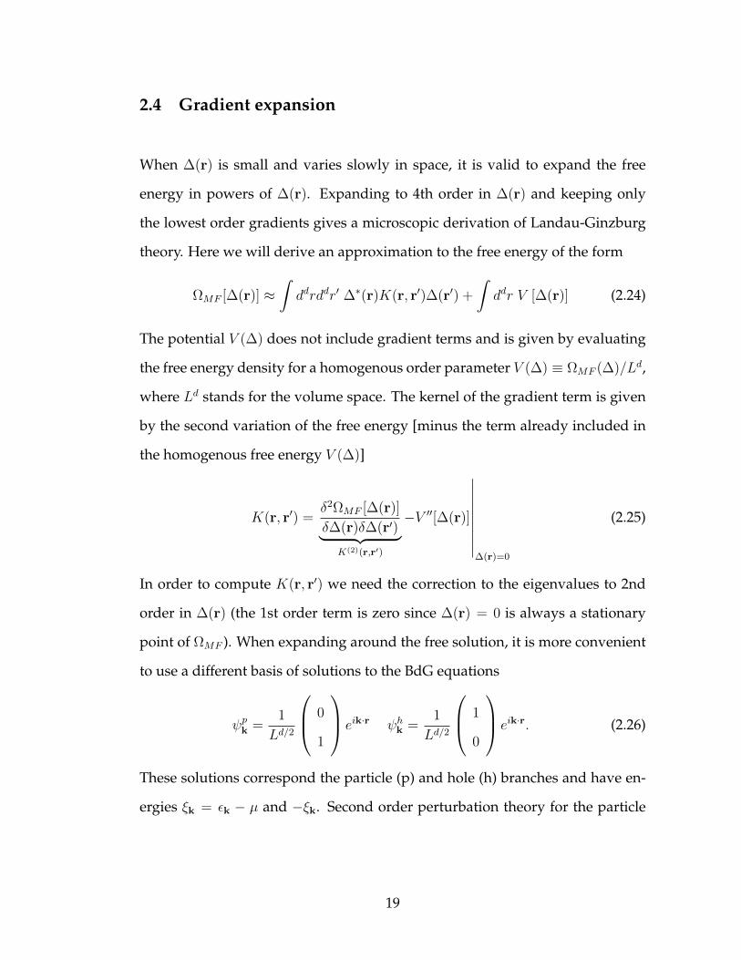
2.4 Gradient expansion

When ∆(r) is small and varies slowly in space, it is valid to expand the free

energy in powers of ∆(r). Expanding to 4th order in ∆(r) and keeping only

the lowest order gradients gives a microscopic derivation of Landau-Ginzburg

theory. Here we will derive an approximation to the free energy of the form

ΩMF [∆(r)] ≈∫ddrddr′ ∆∗(r)K(r, r′)∆(r′) +

∫ddr V [∆(r)] (2.24)

The potential V (∆) does not include gradient terms and is given by evaluating

the free energy density for a homogenous order parameter V (∆) ≡ ΩMF (∆)/Ld,

where Ld stands for the volume space. The kernel of the gradient term is given

by the second variation of the free energy [minus the term already included in

the homogenous free energy V (∆)]

K(r, r′) =δ2ΩMF [∆(r)]

δ∆(r)δ∆(r′)︸︷︷︸K(2)(r,r′)

−V ′′[∆(r)]

∣∣∣∣∣∣∣∣∣∆(r)=0

(2.25)

In order to compute K(r, r′) we need the correction to the eigenvalues to 2nd

order in ∆(r) (the 1st order term is zero since ∆(r) = 0 is always a stationary

point of ΩMF ). When expanding around the free solution, it is more convenient

to use a different basis of solutions to the BdG equations

ψpk =1

Ld/2

0

1

eik·r ψhk =1

Ld/2

1

0

eik·r. (2.26)

These solutions correspond the particle (p) and hole (h) branches and have en-

ergies ξk = εk − µ and −ξk. Second order perturbation theory for the particle

19

energies gives (note that the scalar product (ψp,hk , Vpertψp,hk ) = 0)

δE(2)k =

∑k′

|(ψpk, Vpertψhk′)|2ξk + ξk′

(2.27)

=∑k′

1

ξk + ξk′

∣∣∣∣ 1

Ld

∫ddrei(k

′−k)·r∆(r)

∣∣∣∣2 (2.28)

=∑k′

|∆k−k′|2ξk + ξk′

(2.29)

The change in free energy to 2nd order in ∆(r) (we use again formula (2.23)) is

then

δΩ(2)MF =

∑k,k′

[f(ξ↑k) + f(ξ↓k)− 1]|∆k−k′ |2ξk + ξk′

− 1

g

∫ddr|∆(r)|2 (2.30)

= Ld∑q

K(2)(q)|∆q|2 (2.31)

where we introduced ξσ,k = ξk + σh and

K(2)(q) =1

Ld

∑k

f(ξ↑k+q/2) + f(ξ↓k−q/2)− 1

ξk+q/2 + ξk−q/2− 1

g(2.32)

Note that we shifted momenta k→ k+q/2, k′ → k−q/2 and used the symmetry

q → −q to create a more manifestly symmetric expression. The kernel K(2)(q)

can be used to study instabilities of the normal state towards pairing. A negative

eigenvalue of the kernel signals an instability, i.e. whenever there exists a q such

thatK(2)(q) < 0 the normal state is unstable (Thouless criterion [5]). When such

an instability happens at finite q 6= 0, the normal state is unstable towards a

phase with finite momentum pairing (i.e. the FFLO state [6, 7]) 6. The advantage

of the gradient expansion is that we do not have to solve the complicated BdG

equations. The disadvantages are the limited validity of the approach and the

lack of information about Bogoliubov quasiparticles.

6Of course one needs to be careful here. When such a phase transition is first order, thiscriterion will only give the spinodal line and not the location of the phase transition itself. Inthis case one has to keep higher orders in ∆(r)

20

2.5 Summary

In this chapter we developed the basic theory to describe fermion superfluids

with spin-imbalance. The important tools are

• A formula for the mean-field free energy in terms of eigenvalues of the

BdG equations

ΩMF [∆(r)] =1

2

∑nσ

(εn − µ− 2kBT log

[2 cosh

βEnσ2

])−∫ddr|∆(r)|2g

• The gradient of the free energy functional

δΩMF [∆(r)]

δ∆∗(r)=∑n

u∗n(r)vn(r) [1− f(E↑n)− f(E↓n)] +1

g∆(r)

• A gradient expansion of the free energy

ΩMF ≈∫ddr∆∗(r)K(2)(r− r′)∆(r) +O(∆4) (2.33)

In the next chapter we will solve this theory in various limits to illustrate the

interplay of pairing and spin-imbalance in strongly interacting Fermi gases.

21


[1] P. G. de Gennes, Superconductivity of Metals and Alloys (W.A. Benjamin, NewYork, 1966).

[2] R. P. Feynman, Phys. Rev. 97, 660 (1955).

[3] G. Eilenberger, Z. Physik 184, 427 (1965).

[4] John Bardeen, R. Kümmel, A. E. Jacobs, and L. Tewordt, Phys. Rev. 187, 556(1969).

[5] David J. Thouless, Annals of Physics 10, 553 (1960).

[6] Peter Fulde and Richard A. Ferrell, Phys. Rev. 135, A550 (1964).

[7] A. I. Larkin and Yu. N. Ovchinnikov, Sov. Phys. JETP 20, 762 (1965).

22

CHAPTER 3

APPLICATIONS OF BOGOLIUBOV-DE GENNES THEORY TO

ULTRACOLD ATOMS

3.1 BEC-BCS crossover

The BEC-BCS crossover is parametrized by kFas where kF = (3π2n0)1/3 is the

Fermi momentum in terms of the number density n0 = n↑ + n↓, and as is the

s-wave scattering length. The three different limits that are of interest are

kFas → 0− BCS

kFas → ±∞ unitarity

kFas → 0+ BEC

In the limit of weak attractive interactions as → 0−, there is no bound-state in

vacuum, and the standard BCS theory of Cooper pairing applies. In the oppo-

site regime of strong attractive interactions as → 0+, there exists a deep bound

state of ↑- and ↓-spin atoms in vacuum and these pairs behave like a weakly

interacting gas of bosons. Note that both limits have the same broken gauge

symmetry and this suggests that both limits might in fact be part of the same

phase. In between, in the regime where kFas 1, a weak-coupling description

is not possible. This is the so-called unitary limit, where the scattering ampli-

tude reaches the limit dictated by the requirement that the S-matrix has to be

unitary and we only consider s-wave scattering1. It was realized by Leggett

1To avoid confusion, we would like to emphasize that this clearly does not mean that thereare no cases where interactions are even stronger. For example when considering long-range in-teractions, scattering channels of all angular momenta become important and the total scatteringcross-section can become larger than the contribution from the s-wave channel at unitarity.

23

that a simple mean-field-theory can capture the qualitative physics over the en-

tire crossover regime at T = 0 [1, 2]. Later Nozières, Schmitt-Rink and others,

generalized this mean-field theory to include Gaussian fluctuations, which is

necessary to obtain a correct description of the finite temperature Bose gas in

the BEC limit [3, 4, 5, 6, 7, 8, 9]. In this chapter, we give a short derivation of

the mean-field results at T = 0. In momentum space, the BdG equations for a

uniform superfluid order parameter are ξk ∆0

∆0 −ξk

ukvk

= Ek

ukvk

(3.1)

The positive eigenvalue and the corresponding normalized eigenvector for the

matrix Hamiltonian Eq. (3.1) are

Ek =√ξ2k + ∆2

0 ;

ukvk

=

√

12

+ ξk

2√

∆20+ξ2

k√12− ξk

2√

∆20+ξ2

k

(3.2)

To find the self-consistent solution we have to solve the gap-equation

∆0 =g

Ld

∑k

∆0

2√ξ2k + ∆2

0

(3.3)

As explained in the appendix of chapter 1, in three dimensions we have to re-

place the bare coupling constant with 1/g → m/(4π~2as) − 1/L3∑

k 1/(2εk).

This gives a regularized gap equation, where the interactions are parametrized

by the experimentally measurable scattering length:

m

4π~2as=

∫d3k

(2π)3

(m

~2k2− 1

2√

(εk − µ)2 + ∆20

)(3.4)

Since we want to work at fixed particle number we also need to simultaneously

solve the number equation

n0 =1

L3

∑k

(1− ξk

Ek

)=

∫d3k

(2π)3

1− εk − µ√(εk − µ)2 + ∆2

0

(3.5)

24

The pair of equations (3.4), (3.5) can be brought to the dimensionless form

F1(x0) = −π2αy

1/20 (3.6)

F2(x0) = −2

3y

3/20 (3.7)

where α = (kFas)−1, x0 = µ/∆0, y0 = EF/∆0, and

F1(x0) =

∫ ∞0

dx

(x2√

(x2 − x0)2 + 1− 1

)(3.8)

F2(x0) =

∫ ∞0

dx x2

(x2 − x0√

(x2 − x0)2 + 1− 1

). (3.9)

The results from solving gap and number equations numerically as a function

Figure 3.1: Variation of order parameter ∆ (a) and chemical potential µ (b)as a function of 1/(kFas) from BCS to BEC limit, calculated from mean-fieldtheory. The dashed line in (a) is the BCS limit result for the energy gap∆ ∼ 8e−2eπ/(2kF as). In (b) we have also plotted 1/2 of the two-body bound-stateenergy εB = −~2/(ma2

s) for as > 0 (dashed line).

of the crossover parameter 1/(kFas) are shown in Fig. 3.1. By construction, this

theory must work in the BCS limit, x0 → +∞. In this limit, one finds µ = EF

and the BCS result for the energy gap ∆0 = 8e−2e−π/(2kF as) [2]. In the opposite

limit, x0 → −∞, where one has a Bose gas of tightly bound molecules, one has

µ/EF = −1/2εB/EF + 2kFas/(3π) (εB = ~2/(ma2s) is the two-body binding en-

ergy in vacuum). The chemical potential is just half the binding energy plus a

correction for the interaction between bosons. Within mean-field theory these

25

bosons interact with scattering length aBB = 2as. While this is qualitatively

right and the theory gives the correct result in the extreme limit of noninteract-

ing bosons (as = 0+), a study of the four-body problem showed that actually

aBB = 0.6as [10]. At temperatures much less than the Bose condensation tem-

perature one can describe the system in the BEC limit with a Gross-Pitaevskii

free energy [11, 12]

ΩMF ≈∫d3rφ∗(r)

[−~2∇2

4m− µB

]φ(r) + gBB|φ(r)|4 (3.10)

where gBB = 4π~2aBB/(2m), µB = 2µ+ EB, and the density is of pairs given by

nB(r) = |φ(r)|2. We note that µ goes negative at (kFas)−1 ≈ 0.55. While there

is no phase transition at this point, the minimum of the fermionic excitation

spectrum E(k) shifts to k = 0. The gap in the quasi-particle spectrum is given

by

Egap =

∆0 µ > 0√∆2

0 + µ2 µ < 0(3.11)

Note that ∆0 is not equal to the gap in the fermionic excitation spectrum for

µ < 0. In the BEC limit the energy gap to creating a (pair of) fermionic excita-

tions is equal to EB/2 (EB) respectively. To avoid confusion we will call ∆0 the

superfluid order parameter.

Apart from the BCS and BEC limit, most theoretical and experimental work

has focused on the strongly interacting unitary limit where 1/(kFas) = 0. Since

as is infinite, the scattering cross section at low energies scales as σ ∼ 1/k2 and

the thermodynamics of the system becomes universal [13, 14, 15, 16, 17]. This

lack of a length-scale strongly constraints the thermodynamics functions. For

example, simple dimensional analysis shows the T = 0 energy density ε has to

26

Figure 3.2: Mean-field Bogoliubov excitation spectrum in the BCS (a) and BEC(b) limit (solid lines). Note how the character of the fermionic excitations de-pends on the sign of µ = 0. The dashed lines are the corresponding noninteract-ing spectra with ∆0 = 0.

be proportional to the energy density of a noninteracting Fermi gas ε0 [18]

ε = ξε0 (3.12)

The proportionality constant ξ is a universal many-body parameter2 and its pre-

cise value has received considerable attention, both in experiments [14, 19, 20,

21] and theoretical calculations [13, 15, 22, 23, 24, 25, 26, 27, 28, 29, 30, 31, 32].

The complete T = 0 equation of state is known, once one knows the value of ξ.

Mean-field theory gives an upper bound on the parameter ξ, because the vari-

ational principle implies EMF > E. One finds ξMF = 0.6, whereas Quantum

Monte-Carlo calculations give ξ ≈ 0.41 < ξMF [33] 3. The free energy density

f = Ω/L3 is then expressed as

f = ε− µn = ξε0 − ξ∂ε0∂n

n = ξf0(µ/ξ) = − 2

15π2

(2m

ξ~2

)3/2

µ5/2

where we used f0 = −2(2m/~2)3/2µ5/2/(15π2) for the free energy density of a

noninteracting two species Fermi gas. The number density n = n↑ + n↓ can be

2Sometimes we will use instead the equivalent parameter β = ξ − 1, introduced in [14].3One has µ = ξEF , then we can read off ξMF = 0.6 from Fig. 3.1

27

obtained as

n = −∂f∂µ

=1

3π2

(2mµ

ξ~2

)3/2

(3.13)

This implies that the density profile of a unitary Fermi gas has the shape at T = 0

as that of a noninteracting Fermi gas (up to a scale factor).

3.2 Effect of spin-imbalance — Clogston limit

An interesting tuning knob that is available in experiments with neutral ultra-

cold fermionic atoms is the ability to control spin populations, creating a sce-

nario where N↑ 6= N↓. This is very exciting for several reasons

• In solid state materials, spin imbalance is achieved by putting the sample

in a magnetic field, involving both a vector potential (orbital field) and

a Zeeman field. For a typical superconductor it is the orbital effect that

dominates the physics: either the system expels the field (Meissner phase),

the field penetrates the superconductor via vortex lines (Abrikosov flux

lattice), or superconductivity is destroyed and the system turns normal.

This means it is difficult to study this physics in solid state systems4.

• How does a paired superfluid respond to spin-imbalance? This is a very

old question and many, sometimes exotic, phases have been proposed

where Cooper-pairing and magnetism could coexist [38, 39, 40, 41, 42].

Cold atom experiments allow to study this question in different dimen-

sions and lattice configurations, as well as weak and strong coupling.

4One can suppress the Meissner effect in thin-film or layered or 1D superconductors in aperpendicular magnetic field. In the solid state community such systems have been studiedwith great interest in recent years (see e.g. [34, 35, 36, 37]).

28

• The high-energy and nuclear astrophysics communities are interested in

understanding the phases of high density QCD which could be relevant to

some pulsars. Also neutron-proton pairing in the core of neutron stars has

been discussed [43]. These Fermi superfluids, if they exist, are believed

to involve asymmetric pairing and strong interactions. Both effects can be

simulated in experiments with cold atoms.

In the grand canonical ensemble spin imbalance is achieved by mismatching

chemical potentials, i.e. by adding the Zeeman-term

HZ = h

∫d3r (n↑(r)− n↓(r)) (3.14)

to the Hamiltonian for the balanced gas. We will first discuss what happens

in the weak coupling BCS limit. At zero temperature, the free energy of the

superfluid is unchanged as long as h < ∆0, and the system should definitely be

magnetized for h > ∆0, because in this case the system will become magnetized

through the creation of Bogoliubov quasiparticles (note that these quasiparticles

carry definite spin ↑,↓). To see whether there is a phase transition for a hc <

∆0 we compare the free energy of a noninteracting normal state to that of the

superfluid

fN = − 1

15π2

(2m

~2

)3/2 [(µ+ h)5/2 + (µ− h)5/2

]≈ f0 − h2 mkF

2π2~2(3.15)

When we compare the free energy reduction to the condensation energy Eq.

(3.78), we find that both superfluid and polarized normal state have the same

energy when hc = ∆0/√

2. We should expect a first order phase transition (first

order because hc < ∆0) when the field reaches the critical value h = hc. The

point where it becomes more favorable to create a magnetized normal state

rather than lowering the energy via Cooper pairing is known as the Clogston-

Chandrasekhar or Pauli limit of superconductivity [38, 39]. We can use the

29

mean-field theory to calculate the phase diagram for an imbalanced gas in the

BEC-BCS crossover. For a uniform order parameter ∆(r) = ∆0, the T = 0 free

energy is given by5

ΩMF (∆, h) =1

2

∑k,σ=↑,↓

[εk − µ− |Ek,σ| −

1

2εk

]− m|∆0|2

4πas~2(3.16)

The phase diagram Fig. 3.3 can be found by minimizing of the free energy with

respect to ∆0 at fixed µ, h. The choice of normalization is somewhat nontrivial,

as the obvious unit for energy, ~2/(2ma2s) diverges at unitarity and is symmetric

in as. A useful way to discuss the global phase diagram was put forward by Son

and Stephanov in Ref. [50], were we normalize by the Zeeman field h by the

energy gap (in the fermionic spectrum) Egap and work at fixed µ/∆0, where ∆0

is the order parameter for h = 0. At h = 0, there is then a unique correspondence

between µ/∆0 and kFas. The advantage of this choice of units is that the energy

scale that we use to normalize µ and h stays finite throughout the crossover. The

free energy difference between the state at h = 0 and h 6= 0 is given by

δΩ(∆) = −∑k

(Ek + h) θ(h− Ek) (3.17)

= −L3∆5/20

(2m

~2

)3/2

δ5/2F4(x0/δ) (3.18)

where we introduced δ = ∆/∆0, z0 = h/∆0, and

F4(x0, z0) =

∫ x+

x−

dx x2√

(x2 − x0)2 + 1− z0

3

(x3

+ − x3−). (3.19)

The limits of integration x± =√x0 ±

√z2

0 − 1 are the real positive solutions for

x of the equation z0 =√

(x2 − x0)2 + 1. When there is only one positive solution

x+ > 0, then x− = 0. In the case where there are no real positive solutions we

take x+ = x− = 0. The total free energy is then given by

f(x0, z0, δ) =∆

5/20

2π2

(2m

~2

)3/2

δ5/2

[F3(x0/δ) + F4(x0/δ, z0/δ)−

απ

4

√y0

δ

](3.20)

5We use Eq. (5.5), with 2β−1 log[2 cosh(βE/2)]→ |E| as β ≡ 1/(kBT )→∞.

30

Figure 3.3: Global topology of the mean-field theory phase diagram of the po-larized Fermi-gas at T = 0 [44, 45, 46, 47, 48, 49, 50, 51, 52]. We plot the phase-diagram in the units of Ref. [50], where we practically work at fixed h, µ andnormalize h with the energy gap Egap from Eq. (3.11). Note that we define kFwith reference to the density of the h = 0 superfluid. Many qualitative featuresof this mean-field phase diagram are believed to be correct and have mostlybeen confirmed in experiments [53, 54, 55]. Including interactions in the normalstate shifts the transition line between partially and fully polarized normal tothe right (recent QMC calculations suggest that the line is even shifted beyondthe critical point where the Bose-Fermi mixture becomes a stable phase [51]). Inbrackets we indicate whether a phase is polarized [P = (n↑ − n↓)/(n↑ + n↓)].

with

F3(x0) =

∫ ∞0

dxx2(x2 − x0 −

√(x2 − x0)2 + 1

). (3.21)

We plot this free energy in Fig. 3.6 as a function of δ. In the BCS limit the phase

diagram features a first order phase transition from the unpolarized superfluid

state to a partially polarized Fermi liquid. This picture is still valid at unitarity.

31

In the BEC limit, the phase diagram of the polarized gas can be understood by

mapping the system on a weakly interacting boson-fermion mixture of tightly

bound pairs and unpaired excess fermions [56, 57]. The Hamiltonian for a Bose-

Fermi mixture is

HBF =

∫d3x φ†B(r)

(−~2∇2

4m− µB

)φB(r) +

∫d3x ψ†F (r)

(−~2∇2

2m− µF

)ψF (r)

+gBB

2

∫d3x

[φ†B(r)

]2 [φB(r)

]2

+ gBF

∫d3x φ†B(r)ψ†F (r)ψF (r)φB(r), (3.22)

where φ†B(r) and ψ†F (r) are creation operators for the molecules and excess

fermions, respectively. A Hartree-Fock mean-field decoupling of the Hamil-

tonian Eq. (3.22) yields the free energy density

fBF = − (µB − ΣB)nB +gBB

2n2B −

(2m)3/2

15π2~3(µF − ΣF )5/2 − gBFnBnF . (3.23)

Here the Hartree self-energies are ΣB/F = gBFnB/F and the coupling constants

are related to scattering lengths as gBF = 3~2aBF/m, gBB = 2~2aBB/m. The

simple BdG mean-field theory predicts aBF = 8/3as, whereas a solution to

the three-body problem gives the exact result for the dimer-fermion scattering

length aBF = 1.2as [58, 59]. The phase diagram at finite temperature was exten-

sively studied with a self-consistent Hartree-Fock theory by Sourish Basu in his

Ph.D. thesis [60]. It turns out that the imbalanced Fermi gas behaves in many

ways similar to 4He/3He-3 mixtures [61]. The zero temperature phase diagram6

is shown in Fig. 3.4. At high densities or strong coupling one has a first order

phase transition to a fully polarized (noninteracting) Fermi gas. At the critical

point S a polarized superfluid phase emerges. The transition between super-

fluid and this polarized superfluid is always continuos. Additionally, there is

also a tricritical point T where the transition between normal state and super-

fluid becomes continuous. Before reaching the point S the first order transition6Here shown for the accurate parameters for aBB = 0.6as, aBF = 1.2as. Qualitatively, the

mean-field values result in the same phase diagram.

32

between unpolarized superfluid and fully-polarized normal is found by equat-

ing the normal and superfluid free energies fS = fN , which is equivalent to

− µ2B

2gBB= −

(2m

~2

)3/2µ

5/2F

15π2(3.24)

The superfluid state becomes polarized when µF = gBFnB or

µF = gBFµBgBB

(3.25)

Both Eqs. (3.24),(3.25) are simultaneously satisfied at the point S, with

S = (µB, µF ) =225π4g2

BB~6

32g5BFm

3· (gBB, gBF ) . (3.26)

To find the tricritical point we approach the problem from low density side

where the transition between normal and superfluid is continuos. At the phase

transition we have nB = 0 and

∂fBF∂nB

= 0 (3.27)

Solving for µF we get µF = (~2/m)(3/4π2µB/gBF )2/3 at the second order transi-

tion line. This transition turns first order when

∂f 2BF

∂n2B

∣∣∣∣nB=0

= gBB − g2BF

√µF2

m3/2

π2~3= 0 (3.28)

The tricritical point is then at

T =2π4g2

BB~6

g4BFm

3·(

1,2gBB3gBF

). (3.29)

3.3 Density profiles and phase diagrams

An important probe in experiments with ultra-cold Fermi gases are in-situ den-

sity profiles. These experimental systems are confined by a trapping potential,

33

Figure 3.4: Phase diagram of a Bose-Fermi mixture, calculated from the Hartree-Fock free energy Eq. (3.23). The values of the boson-fermion scattering lengthare aBF = 1.2as and aBB = 0.6as (these parameters differ from the mean-fieldresults and are appropriate for the imbalanced Fermi gas in the BEC limit) [58,59, 10]. The boson (fermion) chemical potentials µB (µF ) are normalized by halfthe binding energy εB/2 = ~2/(2ma2

s) of the pairs.

i.e. experiments probe inhomogeneous systems in an external trapping poten-

tial V (r). For theoretical calculations it is more convenient to calculate prop-

erties of homogenous systems. Typically V (r) varies on a length scale much

longer than the healing length, then a natural assumption is to view the system

as locally homogenous and use the homogenous equation of state, with local

chemical potential

µσ(r) = µcσ − V (r) (3.30)

34

where σ =↑, ↓ labels the spin components. The chemical potentials at the center

µcσ are determined by the total particle numbers

Nσ =

∫d3r nσ(µc↑ − V (r), µc↓ − V (r)) (3.31)

This Thomas-Fermi approximation is also known as local density approxima-

tion (LDA) in the ultra-cold atoms community7. It can also be derived from the

condition of hydrostatic equilibrium of fluids [62]. For a two species Fermi gas it

is convenient to display phase diagrams in terms of the effective Zeeman mag-

netic field h = (µ↑−µ↓)/2 and the average chemical potential µ(r) = (µ↑+µ↓)/2.

In a trapped system the local Zeeman field is independent of position h =

(µc↑ − µc↓)/2, whereas the average chemical potential µ(r) = (µc↑ + µc↓)/2 − V (r)

decreases as one goes towards the edge of the cloud. Hence the trapped system

lives on a straight line of constant h of the phase diagram plotted in the µ, h-

plane. A general feature that can be extracted from experiments is the sequence

of phases observed, e.g. by dividing regions into fully polarized, unpolarized

or partially polarized [53, 63]. In principle there could be multiple phases with

the same density characteristics, but theoretically every phase transition would

be visible as a jump (if first order) or singularity (if second order) in the density

profile. For the phase diagram of the imbalanced unitary Fermi gas at T = 0,

two distinct sequences of phases were proposed [44, 64, 27]. If we assume a

non-interacting normal state, the location of the first order superfluid to normal

phase transition is found by requiring fS = fN or

(1 + η)5/2 + θ(1− η)(1− η)5/2 =2

ξ3/2(3.32)

where η = h/µ and θ(x) is the Heaviside step function. When we assume the

mean-field theory value ξMF = 0.6, one finds ηc ≈ 0.79 < 1, i.e. the phase7So far there are very few known examples where this approximation is not valid. One

expects a break down near a second order phase transition (there one has a diverging length-scale).

35

boundary is between the unpolarized superfluid and a partially polarized nor-

mal state. On the other hand we could try to improve upon mean-field the-

ory by using the more accurate QMC value ξ = 0.42 [64]. This would imply

ηc ≈ 1.22 > 1 and a direct phase transition to the fully polarized normal state

with no partially polarized phase. Early experiments by the Rice group seemed

to support this “two shell model”, whereas the MIT group found three shells

including a partially polarized normal phase [21, 65]. QMC calculations relying

on the fixed-node approximation for the equation of state of the partially polar-

ized normal state later showed that attractive interactions significantly increase

the stability of the normal state [27]. The consequence of these interactions is

that there still is a window of stability for the partially polarized normal state,

consistent with what was observed in the MIT experiments.

3.4 Stability of the Fulde-Ferrell state in D = 3

So far we have not considered any superfluid state that breaks translational

symmetry8. It turns out that in the BCS limit of the imbalanced Fermi gas, a

superfluid with broken translational symmetry appears to be stable [41, 42].

Generically, these Fulde-Ferrell-Larkin-Ovchinnikov (FFLO9) states are both po-

larized and paired at the same time. One should view these states as variational

approximations for the gap parameter ∆(r). The most common approximations

are the FF state introduced by Fulde and Ferrell,

∆FF (r) = ∆0 eiq·r (3.33)

8A classic example for such a state is the Abrikosov vortex lattice phase.9Some authors also call it the LOFF state.

36

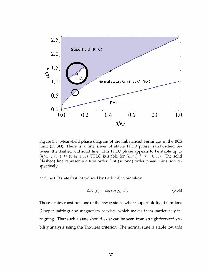
Figure 3.5: Mean-field phase diagram of the imbalanced Fermi gas in the BCSlimit (in 3D). There is a tiny sliver of stable FFLO phase, sandwiched be-tween the dashed and solid line. This FFLO phase appears to be stable up to(h/εB, µ/εB) ≈ (0.42, 1.39) (FFLO is stable for (kFas)

−1 ≤ −0.56). The solid(dashed) line represents a first order first (second) order phase transition re-spectively.

and the LO state first introduced by Larkin-Ovchinnikov,

∆LO(r) = ∆0 cos(q · r). (3.34)

Theses states constitute one of the few systems where superfluidity of fermions

(Cooper pairing) and magnetism coexists, which makes them particularly in-

triguing. That such a state should exist can be seen from straightforward sta-

bility analysis using the Thouless criterion. The normal state is stable towards

37

0.0 0.1 0.2 0.3 0.4 0.5

0.000

0.005

0.010

0.015

(a)(b) (c)

Figure 3.6: (a) Mean-field free energy as a function of the superfluid order pa-rameter δ = ∆/∆0 for a series of Zeeman magnetic fields h/hc = 0, 0.5, 0.8, 1.0at kFas = −1. Note that at the Clogston limit h = hc there appears to be a firstorder phase transition to the normal state when the minima in the free energyare degenerate. (b) Minimum of the kernelK(2)(qmax) (related to the pair suscep-tibility) as a function of interaction strength on the Clogston limit. The normalstate becomes unstable towards FFLO around (kFas)

−1 ≤ −0.56. (c)K(2)(q) plot-ted at fixed interaction strength (kFas)

−1 = −1 at, above and below the Clogstonlimit. (In all figures we have defined kF always via the unpolarized superfluidstate at h = 0)

Cooper pairing if the kernel K(2)(q) from Eq. (2.32) has10

K(2)(q) > 0 for all q (3.35)

For T = 0 and h > 0, K(2)(q) may be evaluated analytically (see S. Basu, Ph.D.

thesis [60]). One obtains

2πK(2)(q) = 2(1 + r) +f ↑+ + f ↑− + f ↓+ + f ↓−

q− 2πiζ − 1/(k↑Fas) (3.36)

f ↑σ =

(q2

4+ ζ2 − 1 + σqζ

)log

(q − 2 + 2σζ

q + 2 + 2σζ

)f ↓σ =

(q2

4+ ζ2 − r + σqζ

)log

(q − 2r + 2σζ

q + 2r + 2σζ

)where K(2) = (4π/mk↑F )K(2), q = |q| /k↑F , r = k↓F/k

↑F , ζ = (1 + r2)/2 − q2/4 and

k↑,↓F =√

2m(µ± h), and for brevity we have set ~ = 1. When µ↑,↓ ≤ 0, one takes

k↑,↓F ≡ 0. Note that for h = 0, K(2)(q → 0) → −∞. The consequence is that the

unpolarized normal state is unstable for an arbitrary weak attractive interaction

at T=0 [66]. At finite Zeeman field, the normal state is not always unstable.

10Note that K(2)(q, µ) is related to the many-body T-Matrix via T−1(q, ω) = K(2)(q, µ− ω).

38

To see in what region the partially polarized normal state is unstable, we plot

the minimum of K(2)(q) at the Clogston limit h = hc as a function of (kFas)−1

(where kF is the h < hc superfluid phase kF ). As can be seen in Fig. 3.6 (b), this

minimum crosses zero around (kFas)−1 = −0.56 (on the BCS side). Below this

critical point, the FFLO phase is stable in a thin sliver around the Clogston limit

and we find the instability of the normal state by finding the field hc1 at which

the minimum of K(2)(q) crosses zero. In the deep BCS limit the ratio hc1/hc =

1.066 is maximal [41, 57]. It is generally believed that the transition from the

normal state towards FFLO is a second order phase transition and in this case

the stability analysis is the same, independent whether the true ground state is

the FF or LO state. Typically, the LO state has a slightly lower energy than the FF

state11. In general the question whether the phase transition from the uniform

superfluid to FFLO is first or second order is nontrivial. The FF (and LO) states

predict a first order transition of the superfluid towards FFLO, approximately

at the Clogston limit (i.e. hc2 = hc) [57]. A scenario for a continuous phase

transition was investigated by Yoshida and Yip [67]. They estimated the Zeeman

field at which a single π-domain wall in the superfluid becomes energetically

stable. It was found that this point occurs earlier than the first order transition

predicted from the FF state, and the authors concluded that the transition of

the superfluid is actually second order starting at polarization P = 0 (this was

already known to be the case in lower dimensions [68, 69]). While the arguments

of Ref. [67] are suggestive of a second order phase transition, there is no proof

that the transition within mean-field theory is indeed second order. If domain

walls interact via attractive interactions, the transition from uniform superfluid

to FFLO would again be first order. Regarding the experimental realization

and detection of FFLO we would like to emphasize that the amount of FFLO

11As we will see it is easier to use the FF state to do calculations.

39

visible in a trapped system is determined by the region occupied by the phase

in the phase diagram plotted in the µ, h-plane. In either scenario this region is

extremely small when considering 3D (or 2D) systems. So far, no signature of an

FFLO phase has been found in an experiment with imbalanced fermions in 3D.

The reason why the FFLO phase inD > 1 has such a small region of stability can

be understood from an analogy to the Peierls instability of the Fermi gas at T =

0. Whenever there is a nesting vector, the normal state is unstable to forming

a charge density wave (CDW) for an arbitrarily weak repulsive interaction. In

(quasi-)1D there is naturally a momentum vector q such that kF,↓+ q = kF,↑. The

consequence is that then the normal state at T = 0 is unstable towards FFLO

at any imbalance and for an arbitrarily weak attractive interaction. In higher

dimension, there is in general no such nesting vector that allows for pairing of

the full Fermi surface at finite momentum and then the normal state will only

be unstable for small imbalance. This is similar for the Peierls instability: When

there is no nesting vector, a finite interaction strength is required to render the

normal state unstable.

3.5 Dark solitons and Andreev boundstates — A toy model for

FFLO

In the limit of low population imbalance, a picture for the FFLO phase is an ar-

ray of well separated π-domain walls [68, 69]. Each of these kinks has a bound-

state close to zero energy, analogous to the Caroli-de Gennes-Matricon (CGM)

bound states found at the core of vortices in superconductors [70, 71, 72, 73].

An applied Zeeman magnetic field spin-polarizes these Andreev boundstates.

40

Figure 3.7: Top: Andreev boundstate wavefunctions (u(z), v(z))T for parametersin the BCS regime (in terms of the dimensionless units described in the text, weused ∆0 = 1, µ = 5, d = 20). (a) Positive energy bound-state solution for a singledomain wall ∆(z) = sign(z)∆0. (b) Symmetric solutions for two domain walls∆(z) = ∆0 (sign(d/2 + z)− sign(z − d/2)− 1). Bottom: (c) Toy model for lowpolarization density FFLO: An array of weakly interacting sharp domain walls.The boundstates, localized at each domain wall, start to overlap and give rise toa bandstructure. (d) Bound state energies for the configuration of two domainwalls in (b), where the distance d between the kinks is varied.

This is the mechanism that allows the superfluid to become polarized in the

FFLO phase. A simple model for such a domain wall is a step-function order

parameter

∆(z) = ∆0 sign(z) (3.37)

It turns out that this model allows for an analytic solution of the Andreev

boundstate. This solution will allow us to understand some generic features

41

of the FFLO phase. The Bogoliubov de Gennes equations are (~2/2m = 1)− d2

dz2 − µ ∆(z)

∆∗(z) −(− d2

dz2 − µ)

un(z)

vn(z)

= En

un(z)

vn(z)

(3.38)

Note that the matrix operator

P =

P 0

0 −P

, (3.39)

where P is the reflection operator with Pψ(z) = ψ(−z), is a symmetry of the

Hamiltonian, i.e. PHP† = H . The consequence is that we can chose the eigen-

functions of H to be eigenfunctions of P as well. Therefore the wavefunctions

un, vn can be chosen to be symmetric, antisymmetric.

We will now look for possible bound state solutions. Therefore we require

E < ∆. The appropriate ansatz for a constant pairing potential isu(z)

v(z)

=

u0

v0

eiwz (3.40)

where w is a c-number. The BdG equations (3.38) for z > 0 reduce tow2 − µ ∆0

∆0 −(w2 − µ)

u0

v0

= E

u0

v0

(3.41)

We find for the eigenvalues

E± = ±√

(w2 − µ)2 + ∆20 (3.42)

and the eigenvectors

ψ± =

u±v±

−(w2 − µ)∓

√(w2 − µ)2 + ∆2

0

∆0

(3.43)

42

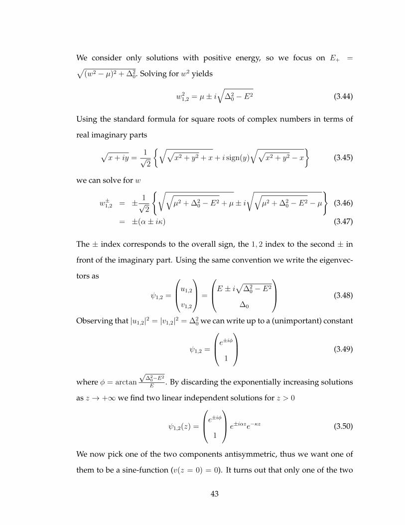
We consider only solutions with positive energy, so we focus on E+ =√(w2 − µ)2 + ∆2

0. Solving for w2 yields

w21,2 = µ± i

√∆2

0 − E2 (3.44)

Using the standard formula for square roots of complex numbers in terms of

real imaginary parts

√x+ iy =

1√2

√√x2 + y2 + x+ i sign(y)

√√x2 + y2 − x

(3.45)

we can solve for w

w±1,2 = ± 1√2

√√µ2 + ∆2

0 − E2 + µ± i√√

µ2 + ∆20 − E2 − µ

(3.46)

= ±(α± iκ) (3.47)

The ± index corresponds to the overall sign, the 1, 2 index to the second ± in

front of the imaginary part. Using the same convention we write the eigenvec-

tors as

ψ1,2 =

u1,2

v1,2

=

E ± i√∆20 − E2

∆0

(3.48)

Observing that |u1,2|2 = |v1,2|2 = ∆20 we can write up to a (unimportant) constant

ψ1,2 =

e±iφ1

(3.49)

where φ = arctan

√∆2

0−E2

E. By discarding the exponentially increasing solutions

as z → +∞we find two linear independent solutions for z > 0

ψ1,2(z) =

e±iφ1

e±iαze−κz (3.50)

We now pick one of the two components antisymmetric, thus we want one of

them to be a sine-function (v(z = 0) = 0). It turns out that only one of the two

43

possibilities work since the bound state is not degenerate

ψR(z) =1

2i(ψ+(z)− ψ−(z)) =

sin(φ+ αz)

sin(αz)

e−κz (3.51)

for the region z < 0 we find a similar result

ψL(z) =

sin(φ− αz)

sin(αz)

eκz (3.52)

The lower component is already continuous as well as its derivative. The up-

per component is already symmetric, continuous and clearly has a continuous

derivative if u′(z)|z=0 = 0, thus we require

d

dzsin(φ+ αz)e−κz|z=0 = 0 (3.53)

This is the condition that determines the bound state energy (would we have

picked the upper component antisymmetric, i.e. φ → −φ, the following equa-

tion would have no positive energy solutions). We can solve for the energy E

α cos(φ)− κ sin(φ) = 0

tan(φ) =α

κ√∆2

0 − E20

E0

=

√√µ2 + ∆2

0 − E20 + µ√√

µ2 + ∆20 − E2

0 − µ

E0 = −µ2

+

√µ2

4+

∆20

2

The bound state energy is not quite zero, but in the weak interacting limit of

small ∆0 it is

E0 =∆2

0

2µ+O(∆4

0)

When we generalize our solution to D = 3, one finds a whole family of bound-

states, parametrized by the transverse momentum vector k⊥. Their energy

44

eigenvalues are

E3D(k⊥) = −µ− k2⊥

2+

√(µ− k2

⊥)2

4+

∆20

2. (3.54)

This dispersion relation is shown in Fig. 3.8. Qualitatively the dispersion rela-

tions behave very differently in the BCS- and BEC-limits. This was noted from

a full BdG calculation by the authors of Ref. [74]. What is remarkable, is that

the simple step potential solution gives qualitatively a very similar result. In

the BCS limit, the energy of the bound state is essentially zero, with a mini-

gap of Emg = ∆0(∆0/µ)/2 and the transverse effective mass of the Andreev in

the domain wall is very large (here E3D(k⊥) ∼ Emg + (k⊥∆0/µ)2/2 + . . ., i.e.

m⊥/m ∼ (µ/∆0)2 1). When the dispersion can be linearized around the

Fermi surface (Andreev approximation), the bound state energy is guaranteed

to be exactly zero, due to a very general index theorem [75]. Then the bound-

states for all k⊥ would be degenerate at zero energy. In the BEC limit, where a

π-soliton would not be stable in equilibrium, E3D(k⊥) ∼ −µ + k2⊥ + . . ., i.e. the

effective mass is essentially the bare mass m⊥ ≈ m.

To achieve a finite polarization density in the thermodynamic limit, we need

a finite density of domain walls. In such a model for FFLO, the boundstates

of these domain walls start to overlap when the length-scale ξ = ~vF/∆0 ∼ d,

where d is the separation between domain walls12. This then gives rise to a

bandstructure in the tight-binding limit for the excess fermions. To see how this

happens we studied the two domain walls depicted in Fig. 3.7. The details of

the solution are given in the appendix to this chapter. Here we just note the

general features. From the solution of the two domain problem we find that the

12In units where ~2/(2m) = 1, we have ξ = 2√mu/∆0. The envelope of u(z), v(z), for the

domain wall in Fig. 3.7a decays as exp(−κ|z|), where κ ≈ ∆0/√

2µ (in the BCS limit). Thereforeu(z), v(z) ∼ e−|z|

√2/ξ.

45

BEC limit BCS limit

Figure 3.8: Dispersion relation of the Andreev boundstate of a π-domain wallin 2D or 3D (units have ~2/(2m) = 1). The dashed line represents the gap toBogoliubov quasiparticle excitations, Egap.

boundstate solution behaves as

E(d)− E0 ∝ ±4ακe−dκ sin(αd) + 2α2e−2dκ (3.55)

where κ ≈ ξ/√

2 = ∆0/√

2µ and α ≈ kF =√

2µ. The bound state energies

depend exponentially weak on the separation d, as is naively expected. The

leading contribution to the tail oscillates with the Fermi wavevector kF . This

concludes our investigation of a simple toy model for FFLO.

From the toy model we learn that

• Kink domain walls in the superfluid order parameter carry bound states

that are close to zero energy in the BCS limit

• Spin polarizing these bound states gives rise to a polarized superfluid state

• An array of domain walls allows for a superfluid with finite polarization

density

• The bound states of these domain walls overlap when their separation

becomes of order of the coherence length ξ and a band-structure of bound

46

states emerges

• It becomes clear that the 1D FFLO state is a fundamentally distinct phase

from the scenario in 2D/3D (assuming the order parameter varies only

along a single direction). In 1D, all Andreev boundstates are occupied,

and the density of excess fermions is exactly given by the wavevector of

the order parameter modulation q = π(n↑− n↓) (in other words, FFLO is a

band insulator for the excess fermions). However in 2D/3D, whatever h,

there are always transverse modes crossing the Fermi energy of the excess

fermions (David Huse dubbed this situation “incommensurate FFLO”’ in

order to distinguish it from the 1D “commensurate FFLO” in 1D).

3.6 Fulde-Ferrell versus Larkin-Ovchinnikov in 1D

We mentioned before that typically the LO state has a lower energy than the FF

state. In this section we present a study of both states in one spatial dimension

at T = 0. In general, mean-field theory is not valid in 1D and it turns out that

the model described by the Hamiltonian

H =

∫dz∑σ

Ψ†σ(z)

(− ~2

2m

d2

dz2− µσ

)Ψσ(z) + g1DΨ†↑(z)Ψ†↓(z)Ψ↓(z)Ψ↑(z) (3.56)

has an exact Bethe ansatz solution [76, 77] (here g1D = −~2/(ma) < 0, with the

1D scattering length a > 0). For now this will not bother us and we pretend BdG

theory provides a good approximation13. Because of a Fermi surface nesting

in 1D, the spin imbalanced normal state is always unstable towards FFLO (at

T = 0). This can be seen from the kernel K(2)1D (pair susceptibility) Eq. (2.32),

13In fact BdG theory seems to work quite well for certain observables in the weak couplinglimit. For an extensive comparison, see e.g. [78].

47

Figure 3.9: Top: (a) Mean-field theory phase diagram of a 1D Fermi gas interact-ing with attractive interactions with scattering length a (we neglected Hartreeshifts). On the black line a π-domain wall has the same energy as the uniformsuperfluid, indicating an instability of the P=0 superfluid towards FFLO. Thered line is the first order phase boundary between superfluid and FF state andthe dashed line is the Clogston limit. (b) Free energy of the FF state as a func-tion of ∆0, q [see Eq. (3.61)] for (h, µ) = (0.56, 1.13)~2/(ma2). Local minima aremarked with a red dot. Bottom: (c) Dispersion relation of Bogoliubov quasi-particles for the FF state ansatz ∆(z) = ∆0e

iqz shown here for the parametersof (b). (d) Self-consistent solutions to the 1D BdG equations for different po-larization densities at fixed µ = 2.25~2/(ma2). In the limit of low polarizationdensity, the FFLO phase consists of separated domain walls and the order pa-rameter achieves the value of the uniform superfluid in between nodes. At largepolarization the magnitude of the order parameter reduces and ∆(z) becomessinusiodal. In this limit ∆(z) closely resembles the LO state.

48

which evaluates to (for µ > h, q > 0)

K(2)1D(q) =

m

~2

arctanh(ki+√A

)− arctanh

(ki−√A

)+ arctanh

(√A

ko+

)√A

−arctanh

(√A

ko−

)√A

+a1D

2

(3.57)

where A = µ− q2/4, ki− = q/2−√µ− h, ko− = −q/2−

√µ+ h, ki+ = min(q/2 +√

µ− h,−q/2 +

√µ+ h), ko+ = max(q/2 +

√µ− h,−q/2 +

√µ+ h), and µ, h =

(2m/~2)µ, h. Note that this function has a divergence at qFFLO = kF↑ − kF↓ =√µ+ h−

√µ− h, i.e. mean-field theory predicts that the polarized normal state

is always unstable towards pairing at finite momentum.

From this stability analysis we expect three stable equilibrium phases in 1D:

• An unpolarized superfluid state

• A partially polarized phase with pairing at finite momentum (FFLO)

• A fully polarized normal state

The FF state is described by the spatially varying order parameter ∆(x) = ∆ eiqx.

With the ansatz u(x)

v(x)

=eikx

Ld/2

uk(q) eiqx/2

vk(q) e−iqx/2

(3.58)

the BdG equations become the simple algebraic equationsξk+q/2 ∆

∆ −ξk−q/2

uk(q)vk(q)

= Ek(q)

uk(q)vk(q)

. (3.59)

Solving the 2× 2 eigenvalue problem one finds the eigenvalues

E±k (q) =ξk+q/2 − ξk−q/2

2±√(

ξk+q/2 + ξk−q/22

)2

+ ∆2 (3.60)

49

Since we are using a specific ansatz for ∆(x), we should variationally minimize

the free energy functional Eq. (2.20) as a function of the variational parameters

∆, q. In terms of ∆ and q the free energy is given by

Ω(∆, q) =1

2

∑k,σ

[εk + εq/2 − µ− |E+

k (q) + σh|]− L |∆|

2

g1D

(3.61)

The calculation of the free energy is analogous to that of the Sarma phase. When

h is larger than the minimum in the dispersion relation mink E+k (q), the state

becomes polarized. In the example from Fig. 3.9 (c), there are two wavevectors,

k<− > k>− , where h = E+k (q). The free energy density f is then expressed as the

1D integrals

f(∆, q) =

∫ k<−

−∞

dk

2π

[εk + εq/2 − µ− E+

k (q)]

+

∫ ∞k>−

dk

2π

[εk + εq/2 − µ− E+

k (q)]

+

∫ k>−

k<−

dk

2π

(εk + εq/2 − µ

)+

1

2πh(k>− − k<−

)+

1

g1D

|∆|2 (3.62)

We compute these integrals numerically, the results for specific parameters are

shown in Fig. 3.9 (b). It turns out that the transition between P = 0 superfluid

and FF state, shown in Fig. 3.9 (a), is a first order phase transition. To find

this transition line we fix µma2/~2 and first calculate the energy of the uniform

superfluid state at q = 0. The energy of the FF state is calculated as a function

of the Zeeman field h14. The Zeeman field h where the free energy of the FF

state matches that of the uniform superfluid marks the location of the first order

phase transition. In the weak coupling limit of large density, the asymptotics

of the free energy of the FF state can be computed analytically. The critical

Zeeman field in this limit is the universal ratio hFF/∆0 = (1 +√

3)/4 = 0.683.

We note that, as is the case in 3D, this field is smaller than the Clogston limit

14To find the finite q minimum of Eq. (3.62) we first perform a line search in ∆ along q =qFFLO = kF↑ − kF↓. With resulting estimates for ∆, q as initial conditions, we use standardminimization algorithms to refine the FF state energy.

50

hc/∆0 = 1/√

2 = 0.707 [69].

While the FF state can be used in calculations to find a reasonable approximation

to phase boundaries, it is physically distinct from the true mean-field theory

FFLO ground state. The main shortcomings of the FF state are

• The excitations of the FF state are gapless Bogoliubov excitations (the true

groundstate has gapped Bogoliubov excitations)

• The FF state has the wrong broken symmetries

• A variational calculation with the FF state (or LO state) predicts a first

order transition from the SF to normal state. This transition is however

believed to be of second order starting with an instability of the superfluid

towards forming a single π-soliton.

In 1D it is numerically feasible to directly solve the full system of BdG equa-

tions, Eqs. (2.7) and (2.12), self-consistently. The BdG equations in 1D (again

neglecting Hartree terms) are given by− ~2

2md2

dz2 − µ+ V (z) ∆(z)

∆∗(z) −(− ~2

2md2

dz2 − µ+ V (z))un(z)

vn(z)

(3.63)

We numerically solve the BdG equations real space by putting the system on a

grid with Ng gridpoints and use a box with of length L periodic boundary con-

ditions. The second derivative operator is represented using a pseudospectral

representation15. The gap equation

∆(z) = g1D

∑n

u∗n(z)vn(z) [1− f(E↑n)− f(E↓n)] (3.64)

15It turns out that using a pseudospectral representation makes it easier to deal with the UVregularization of the gap equation. Alternatively one could also use a lower order method as wedid in Ref. [62], and then match the coupling constant to reproduce the correct order parameter.

51

needs to be regularized. This is because we work with a finite cutoff, limited by

the shortest wavevector or the lattice spacing ∆x = L/Ng in our simulation, the

summation over energies above the cutoff has to be evaluated approximately.

This will lead to a correction of the coupling constant g1D [79]. A good ap-

proximation is to use a semiclassical approximation for the modes above the

momentum cutoff Λ = π(Ng − 1)/L16

∞∑|k|>Λ

u∗k(z)vk(z) ≈∞∑|k|>Λ

∆(z)

2√

[εk − µ(z)]2 + |∆(z)|2

≈ ∆(z)1

2

∞∑|k|>Λ

1

εk − µ(z)

= ∆(z)1

2π

√2m

~2µ(z)arctanh

√2mµ(z)

~2Λ2

where we defined the local chemical potential µ(z) = µ− V (z). With this result

we can rewrite the gap equation as

∆(z) = gR1D(z)Λ∑n

u∗n(z)vn(z) [1− f(E↑n)− f(E↓n)] (3.65)

where the summation is now only over the states included in our numerical sim-

ulation (i.e. below the cutoff). The regularized coupling constant gR1D is related

to the bare coupling constant by

1

gR1D(z)=

1

g1D

− 1

2π

√2m

~2µ(z)arctanh

√2mµ(z)

~2Λ2. (3.66)

Similar regularization schemes were used by various authors, see e.g. [79, 78].

Under the assumption of a continuous order phase transition between FFLO

and SF we can use the numerical solution to the BdG equations to find the phase

boundary. If the phase transition is continuous one expects that at a critical Zee-

man field, the free energy of a single domain wall equals the free energy of

16We assume an odd number of grid points Ng .

52

the uniform superfluid. Numerically we find the phase boundary by calculat-

ing the free energy of a pair of domain walls. In the self-consistent calculation

we seed ∆(z) with a pair of step potential domain walls and fix h such that

all bound states are occupied17. The gap equation Eq. (3.65) is subsequently

iterated to self-consistency. The energy of the domain wall can be written as

ΩDW = Ω(0)DW − h∆N , where the piece Ω

(0)DW includes all eigenvalues in the sum-

mation in Eq. (2.20) except for the sub-gap bound states. In terms of the uniform

superfluid the critical Zeeman field hFFLO is

hFFLO =Ω

(0)DW − ΩSF

∆N(3.67)

The black line between SF and FFLO phases in Fig. 3.9 (a) shows hFFLO(ma2/~2)

as a function of the chemical potential µma2/~2. Note that this line is always at

lower field than the result from the FF ansatz. In the weak coupling limit our

result agrees with the analytics of Ref. [69], who predict hFFLO/∆0 = 2/π. The

slope of the SF to FFLO line is opposite of the same transition line in 3D. This

can be seen directly from the asymptotic result for the weak coupling mean-

field BCS gap ∆0/µ ∼ 8e−πkF a which approaches zero as µ→∞. In 1D, the high

density limit is the weak coupling limit and the low density limit is strongly

coupled. One way to understand this behavior is to consider a δ-function im-

purity in 1D — for any non-zero scattering length, at low energy the reflection

probability approaches unity (in 3D it is the other way round, at low energies

the scattering rate goes to zero). The implication for experiments with harmoni-

cally trapped gases is that at low polarization P , the FFLO phase appears at the

center of the trap. To illustrate this behavior we have solved the BdG equations

for a harmonically trapped 1D system with the results shown in Fig. 3.10.

17We used a pair of domain-walls to satisfy periodic boundary conditions. This approachworks if the separation of the domain walls is much larger than the coherence length.

53

Figure 3.10: Self-consistent solution to the BdG equations in 1D for a harmoni-cally trapped system withN↑ = 70,N↓ = 66, µ(z = 0) = 2.25~2/(ma2). Left: ∆(z)with and without imbalance. Each node in the order parameter corresponds toone excess fermion. Right: Density of up-spins n↑(z) (down-spins n↓(z)) respec-tively. Note that at low polarization the density profile in 1D is inverted withrespect to the 3D scenario. The fully paired phase sits on the inside, whereas theFFLO is visible at the trap center.

Finally we would like to emphasize that while the BdG mean-field theory

approach described here is a reasonable variational approach in the weak cou-

pling limit, it fails miserably in the limit of strong coupling (g1D → −∞). At

strong coupling the ground state of Eq. (3.56) is, as will be discussed later, a

Tonks gas of pairs, whereas mean-field theory would predict a weakly interact-

ing Bose condensate. In that sense we cannot consider the mean-field theory

in 1D as an interpolating scheme that interpolates between weakly interacting

BEC and BCS limits. A quasi-1D model however, where weak tunneling be-

tween tubes is included, does not suffer from these shortcomings. In such a

model the low density limit is effectively three dimensional, thus weakly inter-

acting. In the high density limit the Fermi surface of a quasi-1D model becomes

one-dimensional, therefore also weakly interacting. These considerations jus-

tify our BdG mean-field theory approach for the quasi-1D Fermi gas described

in chapter 5.

54

3.7 Appendix A: Asymptotic expansion for BCS and BEC limit

In this appendix we rederive some basic results for gap and number equation

in special limits [8].

3.7.1 BCS limit

In the weak coupling BCS limit, we have ∆0 → 0. For small ∆0, the number

equation gives simply the free fermion result

n0 =1

3π2

(2m

~2

)3/2

µ3/2 + · · · (3.68)

This means µ ≈ EF . We plug this result into the gap equation and get

π

2kFas=

∫ ∞0

dx

(1− x2√

(x2 − 1)2 + (∆0/EF )2

)(3.69)

We proceed by computing the integral

I1(ε) =

∫ ∞0

dx

(1− x2√

(x2 − 1)2 + ε

)(3.70)

as ε → 0. This is a nice textbook exercise in matched asymptotic expansions. If

we try to put ε = 0, the integral does not converge. This is expected, because

we know from BCS theory that the integral should behave as log(ε). This also

means we can’t Taylor expand the integrand in ε. The integral is sharply peaked

around x = 1, so we might try approximate the integrand on an interval (1 −

δ, 1 + δ) around the singularity (where δ is some cutoff)

Ii(ε, δ) =

∫ 1+δ

1−δdx

(1− x2√

(x2 − 1)2 + ε

)=

∫ δ

−δdy

(1− (1− y)2√

((1 + y)2 − 1)2 + ε

)

≈∫ δ

−δ

(1− 1√

4y2 + ε

)≈ 2δ − log

4δ√ε

55

If we approximate I ≈ Ii we get ∆/EF = 4δe−2δeπ/(2kF as). This is reminiscent

of BCS theory, where one typically chooses the Debye frequency as high-energy

cutoff. Here we can do a better job since we precisely know the interaction

between fermions. We split I(ε) into three parts: two outer regions, and an

inner region around the singularity at x = 1

I1(ε) = I<o (ε, δ) + Ii(ε, δ) + I>o (ε, δ) (3.71)

In the outer regions we can Taylor expand the integrand in ε

1− x2√(x2 − 1)2 + ε

≈ 1− x2

|x2 − 1| +x2ε

2((x2 − 1)2)3/2

+O(ε2)

The outer integrals

I<o (ε, δ) =

∫ 1−δ

0

dx

(1− x2√

(x2 − 1)2 + ε

)(3.72)

I>o (ε, δ) =

∫ ∞1+δ

dx

(1− x2√

(x2 − 1)2 + ε

)(3.73)

can then be done analytically to order ε. This approximation is uniformly valid

if ε δ2 1, so we can e.g take δ = ε1/3 to satisfy this condition as ε → 0.

Putting all pieces together and putting δ ≡ ε1/3 we get to leading order in ε

I1(ε) ≈ 2 + log(√ε/8) (3.74)

This gives the well known analytic result ∆/EF = 8e−2eπ/(2kF as) in the BCS limit.

From Fig. 3.1 we see that the formula is a good approximation to the numerical

solution of the full mean-field theory already for kFas ≤ −1. This justifies to

some extent why many experiments consider kFas ∼ −1 to be in the BCS limit.

From the asymptotic expansion for the gap equation Eq. (3.74) can be integrated

to give an approximation for the energy. For a uniform order parameter, the

56

mean-field energy is given by

ΩMF (∆0) =∑k

[εk − µ− Ek −

1

2εk

]− m

4πas~2|∆0|2 (3.75)

≈ EF(LkF )3

2π2

[I2

(∆2

0

E2F

)− π

4kFas

(∆0

EF

)2]

(3.76)

with

I2(ε) ≈ 3

4ε+

ε

2log

√ε

8− 4

15(3.77)

When we evaluate the free energy at its minimum (where 2 + log(√ε/8) =

π/(2kFas)), we get

ΩMF (∆0)− ΩMF (∆0 = 0) = −(LkF )3

8π2

∆20

EF(3.78)

where we subtracted the noninteracting energy of a two-species Fermi gas

ΩMF (∆0 = 0) = −2EF (LkF )3/(15π2). The energy of the condensed state is lower

by an energy gain proportional to ∆20.

3.7.2 BEC limit

In the BEC limit (|µ| ∆0; µ < 0), the perturbation expansion of the momentum

integrals is non-singular, so we use a Taylor series expansion in (∆0/µ)2

n0(µ,∆0) =

(−2mµ

~2

)3/21

16π

[(∆0

µ

)2

− 3

32

(∆0

µ

)4

+ · · ·]

1

4πas=

1

4π

(−2mµ

~2

)1/2[

1 +1

16

(∆0

µ

)2

+ · · ·]

We would like to find expansion for µ/EF in the small parameter 1/kFas. To

do this we write gap and number equations in a dimensionless form with ε =

57

(∆0/µ)2

(−EFµ

)3/2

=3

16π

(ε− 3

32ε2 + · · ·

)(3.79)(

− εB2µ

)3/2

= 1 +ε

16+ · · · (3.80)

where εB = ~2/(ma2s) is the binding energy of two fermions in vacuum. To

leading order we find that µ = −εB/2 (or µ/EF ≈ −1/(kFas)2) which means

that for tightly bound dimers, the energy to add one fermion is just half the

binding energy, as expected. Solving Eqs. (3.79) and (3.80) perturbatively for

δµ = µ+ εB/2 we find

µ ≈ −εB/2 + δµ = EF

(− 1

(kFas)2+

2

3πkFas + · · ·

)(3.81)

Similarly one finds

∆0 ≈ EF

√16

3π

1

(kFas)1/2+ · · · (3.82)

In the deep BEC limit 0 < kFas 1, mean-field theory describes the tightly

bound dimers as a weakly interacting Bose gas. Twice the chemical potential

difference 2δµ should be interpreted as the boson chemical potential µB. For the

weakly interacting Bose gas, µB is given by

µB =4π~2aBBnB

mB

= 2δµ =π~2asn0

m(3.83)

Here aBB is the the boson-boson scattering length and nB = 2n0 (mB = 2m) is

the density (mass) of pairs respectively. From the mean-field theory we obtain

the prediction aBB = 2as18

18As it turns out, this prediction is not quite correct. A solution of the dimer-dimer scatteringproblem predicts aBB = 0.6as [10, 8, 56].

58

3.8 Appendix B: Andreev boundstates for two domain walls

Here we describe our solution to the BdG equations of two step potential do-

main walls located at z = ±d/2. This problem serves as a toy model for the

FFLO state in 1D. We assume that the nodes of the order parameter are at

z = ±d/2 and ∆(z) = ∆0 > 0 in between. By reflection symmetry we only

need to consider one boundary condition (b.c.) at z = d/2 (at z = −d/2 the b.c.

will automatically be satisfied). There are four linear independent solutions that

we choose to be real

ψ1(z) =

cos(φ+ αz)

cos(αz)

e−κz ψ2(z) =

sin(φ+ αz)

sin(αz)

e−κz

ψ3(z) =

cos(αz − φ)

cos(αz)

eκz ψ4(z) =

sin(αz − φ)

sin(αz)

eκz

First we consider the solutions with even parity. The solutions in the middle

region −d/2 < z < d/2 are then

ψ1s(z) = ψ1(z) + ψ3(z) ψ2s(z) = ψ2(z)− ψ4(z)

In the region z > d/2 we discard the exponentially increasing solutions

φ1(z) =

cos(φ+ α(z − d/2))

− cos(α(z − d/2))

e−κ(z−d/2) φ2(z) =

sin(φ+ α(z − d/2))

− sin(α(z − d/2))

e−κ(z−d/2)

Continuity at z = d/2 implies

Aψ1s(d/2) +Bψ2s(d/2) = Cφ1(d/2) +Dφ2(d/2)

Aψ′1s(d/2) +Bψ′2s(d/2) = Cφ′1(d/2) +Dφ′2(d/2)

where A,B,C,D are c-number constants. These equations have nontrivial solu-

tions when the determinant of the 4×4 coefficient matrix vanishes. One obtains

59

the transcendental equation

(α cos(φ) + κ sin(φ))(α cos(φ)− κ sin(φ)) = −8e−dκακ sin(αd) + 4e−2dκα2 (3.84)

For d → ∞ the right hand side is zero and the left hand side is just the product

of the equations for the negative and positive single domain wall boundstate

energies. Similarly, the eigenvalue equation for odd parity is

(α cos(φ) + κ sin(φ))(α cos(φ)− κ sin(φ)) = 8e−dκακ sin(αd) + 4e−2dκα2 (3.85)

One can extract the asymptotics for large d by expanding the equation on the

left hand side around the single domain wall energyE0 and evaluating the right

hand side atE = E0. On the BCS side the solutions oscillate with an exponential

decaying envelope ∼ e−dκ, but in the sum of both positive energies the oscilla-

tions cancel at large distance and the decay is faster ∼ e−2dκ.

60


[1] D. M. Eagles, Phys. Rev. 186, 456 (1969).

[2] A. J. Leggett, in Modern Trends in the Theory of Condensed Matter, edited byA. Pekalski and J. Przystawa (Springer-Verlag, Berlin, 1980), p. 14.

[3] Journal of Low Temperature Physics 59, 195 (1985), 10.1007/BF00683774.

[4] M. Drechsler and W. Zwerger, Annalen der Physik 504, 15 (1992).

[5] R. Haussmann, 91, 291 (1993), 10.1007/BF01344058.

[6] C. A. R. Sá de Melo, Mohit Randeria, and Jan R. Engelbrecht, Phys. Rev.Lett. 71, 3202 (1993).

[7] R. Haussmann, Phys. Rev. B 49, 12975 (1994).

[8] M. Randeria, in Bose-Einstein Condensation, edited by A. Griffin, D. W.Snoke, and S.Stringari (Cambridge University Press, Cambridge, 1995), p.35.

[9] Y. Ohashi and A. Griffin, Phys. Rev. A 67, 033603 (2003).

[10] D. S. Petrov, C. Salomon, and G. V. Shlyapnikov, Phys. Rev. Lett. 93, 090404(2004).

[11] E. P. Gross, Nuovo Cimento 20, 454 (1961).

[12] L. P. Pitaevskii, Sov. Phys. JETP 13, 451 (1961).

[13] Henning Heiselberg, Phys. Rev. A 63, 043606 (2001).

[14] K. M. O’Hara, S. L. Hemmer, M. E. Gehm, S. R. Granade, and J. E. Thomas,Science 298, 2179 (2002).

[15] J. Carlson, S.-Y. Chang, V. R. Pandharipande, and K. E. Schmidt, Phys. Rev.Lett. 91, 050401 (2003).

[16] G. M. Bruun, Phys. Rev. A 70, 053602 (2004).

61

[17] Tin-Lun Ho, Phys. Rev. Lett. 92, 090402 (2004).

[18] G. A. Baker, in Proceedings of the Tenth International Conference on RecentProgress in Many-Body Theories, edited by R.F. Bishop et al. (World Scien-tific, Singapore, 2000).

[19] M. Bartenstein, A. Altmeyer, S. Riedl, S. Jochim, C. Chin, J. Hecker Den-schlag, and R. Grimm, Phys. Rev. Lett. 92, 120401 (2004).


[21] Guthrie B. Partridge, Wenhui Li, Ramsey I. Kamar, Yean An Liao, and Ran-dall G. Hulet, Science 311, 503 (2006).

[22] A. Perali, P. Pieri, and G. C. Strinati, Phys. Rev. Lett. 93, 100404 (2004).

[23] G. E. Astrakharchik, J. Boronat, J. Casulleras, and S. Giorgini, Phys. Rev.Lett. 93, 200404 (2004).

[24] S. Y. Chang, V. R. Pandharipande, J. Carlson, and K. E. Schmidt, Phys. Rev.A 70, 043602 (2004).

[25] J. Carlson and Sanjay Reddy, Phys. Rev. Lett. 95, 060401 (2005).

[26] Qijin Chen, Jelena Stajic, Shina Tan, and K. Levin, Physics Reports 412, 1(2005).

[27] C. Lobo, A. Recati, S. Giorgini, and S. Stringari, Phys. Rev. Lett. 97, 200403(2006).

[28] H. Hu, P. D. Drummond, and X.-J. Liu, Nature Phy 3, 469 (2007).

[29] Martin Y. Veillette, Daniel E. Sheehy, and Leo Radzihovsky, Phys. Rev. A75, 043614 (2007).

[30] Yusuke Nishida and Dam Thanh Son, Phys. Rev. A 75, 063617 (2007).

[31] Peter Arnold, Joaquín E. Drut, and Dam Thanh Son, Phys. Rev. A 75, 043605(2007).

62

[32] R. Haussmann and W. Zwerger, Phys. Rev. A 78, 063602 (2008).

[33] S. Gandolfi, K. E. Schmidt, and J. Carlson, Phys. Rev. A 83, 041601 (2011).

[34] X. S. Wu, P. W. Adams, and G. Catelani, Phys. Rev. B 74, 144519 (2006).

[35] Y. L. Loh, N. Trivedi, Y. M. Xiong, P. W. Adams, and G. Catelani, ArXive-prints (2011).

[36] S. Uji, T. Terashima, M. Nishimura, Y. Takahide, T. Konoike, K. Enomoto,H. Cui, H. Kobayashi, A. Kobayashi, H. Tanaka, M. Tokumoto, E. S. Choi,T. Tokumoto, D. Graf, and J. S. Brooks, Phys. Rev. Lett. 97, 157001 (2006).

[37] H. A. Radovan, N. A. Fortune, T. P. Murphy, S. T. Hannahs, E. C. Palm,S. W. Tozer, and D. Hall, Nature 425, 51 (2003).

[38] A. M. Clogston, Phys. Rev. Lett. 9, 266 (1962).

[39] B. S. Chandrasekhar, Applied Physics Letters 1, 7 (1962).

[40] G. Sarma, J. Phys. Chem. Solids 24, 1029 (1963).



[43] Roberto Casalbuoni and Giuseppe Nardulli, Rev. Mod. Phys. 76, 263 (2004).

[44] Paulo F. Bedaque, Heron Caldas, and Gautam Rupak, Phys. Rev. Lett. 91,247002 (2003).

[45] K. B. Gubbels, M. W. J. Romans, and H. T. C. Stoof, Phys. Rev. Lett. 97,210402 (2006).

[46] Masudul Haque and H. T. C. Stoof, Phys. Rev. A 74, 011602 (2006).

[47] C.-H. Pao, Shin-Tza Wu, and S.-K. Yip, Phys. Rev. B 73, 132506 (2006).

[48] Daniel E. Sheehy and Leo Radzihovsky, Phys. Rev. Lett. 96, 060401 (2006).

[49] T. N. De Silva and E. J. Mueller, Phys. Rev. A 73, 051602 (2006).

63

[50] D. T. Son and M. A. Stephanov, Phys. Rev. A 74, 013614 (2006).

[51] S. Pilati and S. Giorgini, Phys. Rev. Lett. 100, 030401 (2008).

[52] M. Punk, P. T. Dumitrescu, and W. Zwerger, Phys. Rev. A 80, 053605 (2009).

[53] Yong-Il Shin, Christian H. Schunck, Andre Schirotzek, and Wolfgang Ket-terle, Nature 451, 689 (2008).

[54] Yong-Il Shin, Andre Schirotzek, Christian H. Schunck, and Wolfgang Ket-terle, Realization of a strongly interacting Bose-Fermi mixture from a two-component Fermi gas, 2008.

[55] S. Nascimbène, N. Navon, K. J. Jiang, L. Tarruell, M. Teichmann, J. McK-eever, F. Chevy, and C. Salomon, Phys. Rev. Lett. 103, 170402 (2009).

[56] P. Pieri and G. C. Strinati, Phys. Rev. Lett. 96, 150404 (2006).

[57] Daniel E. Sheehy and Leo Radzihovsky, Ann. Phys. (NY) 322, 8 (2007).

[58] G.V. Skorniakov and K. A. Ter-Martirosian, Sov. Phys. JETP 4, 648 (1957).

[59] D. S. Petrov, Phys. Rev. A 67, 010703 (2003).

[60] Sourish Basu, Ph.D. thesis, Cornell University, 2009.

[61] E. H. Graf, D. M. Lee, and John D. Reppy, Phys. Rev. Lett. 19, 417 (1967).

[62] Stefan K. Baur, Sourish Basu, Theja N. De Silva, and Erich J. Mueller, Phys.Rev. A 79, 063628 (2009).

[63] Yean-an Liao, Ann Sophie C. Rittner, Tobias Paprotta, Wenhui Li,Guthrie B. Partridge, Randall G. Hulet, Stefan K. Baur, and Erich J. Mueller,Nature 467, 567 (2010).

[64] F. Chevy, Phys. Rev. Lett. 96, 130401 (2006).

[65] Martin W. Zwierlein, Andre Schirotzek, Christian H. Schunck, and Wolf-gang Ketterle, Science 311, 492 (2006).

[66] David J. Thouless, Annals of Physics 10, 553 (1960).

64

[67] Nobukatsu Yoshida and S.-K. Yip, Phys. Rev. A 75, 063601 (2007).

[68] A. I. Buzdin and V. V. Tugushev, Sov. Phys. JETP 58, 428 (1983).

[69] Kazushige Machida and Hiizu Nakanishi, Phys. Rev. B 30, 122 (1984).

[70] C. Caroli, P. G. De Gennes, and J. Matricon, Physics Letters 9, 307 (1964).



[73] Joel D. Shore, Ming Huang, Alan T. Dorsey, and James P. Sethna, Phys. Rev.Lett. 62, 3089 (1989).

[74] Mauro Antezza, Franco Dalfovo, Lev P. Pitaevskii, and Sandro Stringari,Phys. Rev. A 76, 043610 (2007).

[75] Constantine Callias, Communications in Mathematical Physics 62, 213(1978), 10.1007/BF01202525.

[76] M. Gaudin, Phys. Lett. 24A, 55 (1967).

[77] C. N. Yang, Phys. Rev. Lett. 19, 1312 (1967).

[78] Xia-Ji Liu, Hui Hu, and Peter D. Drummond, Phys. Rev. A 76, 043605(2007).

[79] Marcella Grasso and Michael Urban, Phys. Rev. A 68, 033610 (2003).

65

CHAPTER 4

DEFORMED CLOUDS OF IMBALANCED FERMIONIC SUPERFLUIDS

This chapter was adapted from "Theory of the Normal/Superfluid interface in popula-

tion imbalanced Fermi gases " by Stefan K. Baur, Sourish Basu, Theja N. De Silva and

Erich J. Mueller, published in Physical Review A 79, 063628 (2009).

4.1 Abstract

We present a series of theoretical studies of the boundary between a superfluid

and normal region in a partially polarized gas of strongly interacting fermions.

We present mean-field estimates of the surface energy in this boundary as a

function of scattering length. We discuss the structure of the domain wall, and

use a previously introduced phenomonological model to study its influence on

experimental observables. Our microscopic mean-field calculations are not con-

sistent with the magnitude of the surface tension found from our phenomono-

logical modelling of data from the Rice experiments. We conclude that one must

search for novel mechanisms to explain the experiments.

4.2 Introduction

What happens when one tries to polarize a fermionic superfluid? Experiments

at MIT and Rice have shown that when the fermions are interacting via resonant

short range interactions, the fluid responds by phase separating into a largely

unpolarized superfluid region and a less polarized normal region [1, 2, 3, 4, 5].

66

The Rice experiments [1, 2] show a dramatic distortion of the central super-

fluid region in their trapped gas, pointing to significant surface tension in the

boundary. Here we present a theoretical study of this boundary and discuss the

consequences of surface tension.

The phase separation seen in these experiments arises because a zero temper-

ature conventional s-wave superfluid is unable to accommodate spin polariza-

tion: all of the atoms in one spin state (↑) are paired with atoms of the opposite

spin (↓). Changing the density ratio n↑/n↓ from unity requires adding sufficient

energy to break these pairs. Consequently, when excess particles of one spin

state are added to a paired atomic cloud, those particles simply float to the sur-

face, forming a normal fluid. Given that there is a sharp boundary between

the superfluid and normal region, the order parameter must vary rapidly, pro-

ducing a surface energy. In section 4.3 we use the Bogoliubov-de-Gennes(BdG)

equations as a microscopic theory of this interface, and extract a dimensionless

measure of the surface tension η.

In addition to the phase separation scenario seen in experiments, which was

essentially predicted by Clogston and Chandrasekhar [6, 7], there have been

many theoretical proposals for how the superfluid can accommodate extra spins

[8, 9, 10, 11, 12, 13, 14, 15, 16, 17, 18, 19, 20, 21, 22, 23, 24, 25, 26, 27]. We will make

some comments on one class of states, the “FFLO" states introduced by Fulde,

Ferrell, Larkin and Ovchinnikov [8, 9] where polarization resides in a periodic

array of nodes in the superfluid order parameter, or is accommodated by creat-

ing supercurrents. Our mean field approach is sufficiently general that if such

a phase existed in the parameter regime that we discuss, we could observe it.

Like the experiments, and previous mean-field calculations [28], we see no sign

67

of this phase near unitarity (where the scattering length is infinite). Interest-

ingly, a recent density functional calculation [29] raises the possibility that the

mean-field theory may be underestimating the stability of the FFLO state. We

anticipate that in the near future more sophisticated numerical techniques will

be able to unambiguously address the presence of the FFLO state.

Like other theoretical calculations based upon the Bogoliubov de Gennes

equations[30, 31, 32, 33, 34, 35, 36, 37, 38] we find that the order parameter and

polarization oscillate in the domain wall separating the two regions. These oscil-

lations, which in no way should be interpreted as an intervening phase [36], are

small at unitarity, but become larger as one approaches the BCS limit (small and

negative scattering length a). At sufficiently small negative scattering length the

decay length of these oscillations diverge, signaling the onset of the bulk FFLO

phase. The topology of the phase diagram of polarized fermions [22, 39] at zero

temperature features tricritical points in both the BEC (1/kfa 1) and BCS

(−1/kfa 1) limit, where the first order phase transition between superfluid

and normal state turn second order. As surface tension vanishes at the tricritical

points, it reaches a maximum in the crossover region.

In section 4.4 we explore the consequences of surface tension on the shape

of the superfluid-normal boundary for a unitary gas in an anisotropic harmonic

trap. As in previous work [40, 41, 42] we use a simple elastic model for the

boundary. By expanding the shape of the boundary in a Fourier series, we are

able to compare its detailed structure with that of experiments. While our model

appears to capture a great many of the experimental features, it yields sharper

density features. We attribute the discrepancies to the fact that we model the

trapping potential as harmonic.

68

This method complements the approach of Natu and Mueller [42] where the

conditions of hydrostatic equilibrium were used to derive a differential equation

for the boundary. Like Haque et al. [41], we find that as one increases the surface

tension, the boundary distorts from an ellipse into a “capsule-like” shape. The

most relevant experiments, performed at Rice in 2006 [2], use small numbers of

particles in a highly anisotropic trap. Due to the large surface area to volume ra-

tio these experiments observe large distortions, consistent with surface tension

which is one order of magnitude larger than predicted by our microscopic argu-

ments. This behavior should be contrasted with experimental studies at MIT [5]

which find no observable distortion of the superfluid-normal boundary. Taking

into account the much smaller surface area to volume ratio in these experiments,

this null observation bounds η to be not much larger than the value we calcu-

late. We have no explanation for this apparent discrepancy. It is undoubtedly

related to the fact that the Rice experiment finds a normal fluid whose local po-

larization is almost 100%, while the normal fluid seen at MIT is always partially

polarized, even at the lowest temperatures.

4.2.1 Background

In the experiments of interest, fermionic alkali atoms (typically 6Li) are trapped

in a nominally harmonic optical potential. The atoms are transferred into two

collisionally stable hyperfine states so that no spin relaxation occurs on the

timescale of the experiment: the number of particles in each of the two spin

states are separately conserved. Due to the short range nature of the inter-

actions, at sufficiently low temperature scattering is forbidden between two

fermions in the same spin state. Hence interactions can be parameterized by

69

a single scattering length a, which is a function of the applied magnetic field

[43, 44].

For a < 0 the low energy scattering is attractive, and at low temperature the

spin balanced system is a BCS superfluid. For a > 0 the low energy scatter-

ing is repulsive, however there exists a two-body bound state in vacuum. The

low temperature phase in this case is a Bose condensate of pairs. One of the

remarkable predictions born out by experiments is that these two superfluid

phases are continuously connected to one another [45, 46, 47, 48, 49, 4, 5, ?].

Most interest has focused around the unitary point (a = ±∞) where the scat-

tering cross-section is maximal and in free space there exists a bound state at

threshold. At this point the interactions do not provide a length-scale to the sys-

tem, leading to universal thermodynamics where all thermodynamic functions

can be expressed in terms of a power of the density times a universal function of

the density scaled by the thermal wavelength nΛ3 and the spin imbalance n↑/n↓

[50, 51, 52, 53, 54]. In particular, if in the absence of a trap there is a flat phase

boundary between a superfluid and a normal region, with equal pressures on

each side of the boundary, we showed in [40] that any surface tension can be

written as

σ = η~2

2mn4/3s (4.1)

where ns is the density on the superfluid side of the boundary. A completely

equivalent parameterization was later used by Haque and Stoof [41],

σ = ηsm

~2µ2. (4.2)

To convert between the two parameterizations one needs to know the equations

of state of the superfluid – which on dimensional grounds has the simple form

ns(µ) = n↑ + n↓ =1

3π2[

2m

~2(1 + β)µ]3/2, (4.3)

70

where µ is the average chemical potential and β is a dimensionless universal

many body parameter [50, 51, 53, 54]. According to quantum Monte-Carlo cal-

culations β ≈ −0.58 [52, 55, 56, 57, 58], which gives η = 8.1ηs.

If, as in the experiments, the boundary is curved, one expects to observe

a pressure drop related to the curvature [42]. In that case, the dimensional

argument leading to Eq. (4.1) yields an extra parameter, and one must take

η = η(∆p/p) to be a function of the relative pressure drop. As in all previous

treatments, we will neglect the ∆p dependence of this parameter.

The presence of a superfluid-normal phase boundary for the trapped gas is

understood by examining the finite temperature phase diagram of a uniform

Fermi gas, as sketched in figure 4.1(a) in the polarization-temperature plane. At

zero temperature the superfluid and normal state are separated by a polariza-

tion driven first order phase transition. Since the polarization changes discon-

tinuously, there is a “forbidden region" analogous to the one occurring in the

density-temperature phase diagram for a liquid-gas phase transition. The lo-

cation of the phase boundaries are found by a standard Maxwell construction,

where the pressures (free energies) of the two phases are equated. When placed

in a fixed volume (or confined by a harmonic trap) this first order phase transi-

tion leads to a regime of phase coexistence, just as in the more familiar situation

of a liquid-vapor transition.

This first order phase transition is only found at sufficiently low tempera-

tures. There is a tricritical point, above which the boundary becomes a contin-

uous second order line. This behavior is consistent with the standard model of

an unpolarized superfluid, which has a temperature driven second order phase

transition. This structure was experimentally mapped out in [5].

71

Figure 4.1: Schematic phase diagram of a two component Fermi gas as a func-tion of (a) Temperature [T ] - Polarization [P = (n↑ − n↓)/(n↑ + n↓)], (b) Tem-perature [T ] - chemical potential difference [h = (µ↑ − µ↓)/2], and (c) chemicalpotential [µ = (µ↑−µ↓)/2] - chemical potential difference [h = (µ↑−µ↓)/2]. Theequation of state sets a relationship between P, T, h, and µ, so only three of themare needed to specify the state. Solid lines: continuous phase transitions; dashedlines: discontinuous; these meet at the tricritical point [Pt, ht, Tt] or [µt, ht, Tt].The gray region in (a) maps onto the dashed line in (b), and represents a coex-istence region. On the BCS side of resonance a < 0, and for sufficiently largea, P1=0 and 0 < P2 < 1. When a > 0 decreases in magnitude, P1 and P2 moveto the right, sequentially hitting the maximum allowed value P = 1. At uni-tarity, a = ∞, a Wilsonian RG theory[59] predicts Pt = 0.24 and Tt/TF,↑ = 0.06.Monte-Carlo calculations suggest Tc/TF = 0.152(7)[60], and P2 = 0.39[58].

72

In figure 4.1(c) the same diagram is shown at fixed temperature as a function

of the chemical potentials µ = (µ↑ + µ↓)/2 and h = (µ↑ − µ↓)/2. As a first

approximation, one understands the trapped gas by breaking up the cloud into

small pieces, and assuming that at each of these pieces is homogeneous and in

local equilibrium. Maintaining equilibrium in the presence of energy transport

requires T is constant, allowing momentum transport requires that the pressure

obeys∇P = −n∇V , where V (r) is the trapping potential, and allowing particle

transport requires ∇µj = −∇V for j =↑, ↓. This hydrodynamic, Thomas-Fermi

description allows one to directly read the structure of the trapped gas from the

homogeneous phase diagram in figure 4.1(c): h is constant and µ varies from a

large value at the center of the cloud to a small value at the edge. The iso-density

contours of the cloud follow the iso-potential contours.

Observations at Rice are inconsistent with this local density approximation

[61]. As already emphasized, the missing element is that the surface energy

described in Eq. (4.1) distorts the cloud. Microscopically, this surface tension

arises due to the energy cost of the superfluid-normal boundary, where the or-

der parameter varies rapidly. Depending on the size of the superfluid region

it is energetically favorable to either shrink this boundary to reduce its area or,

because the surface energy depends on density, shift the boundary to a low den-

sity region. In a spherical trap this effect changes the radius (and density) of the

superfluid core. In an elongated cloud, one generically expects that the aspect

ratio of the superfluid region is reduced. Phenomenological models based on

this principle [40, 41], seem to account for the experimental observations.

By fitting various models to experimental density profiles, Haque and Stoof

[41] and DeSilva and Mueller [40] both made an estimate of η. The quoted val-

73

ues of η in [40] were unintentionally scaled by a factor of ~ωz/µ0. When cor-

rected for this factor, they found that η ≈ 0.6 for the relatively high temperature

data in [1]. Haque and Stoof [41] found η ≈ 4.8 for the lower temperature data

in [2]. This is consistent with the expectation that surface tension should drop

as one approaches the tricritical point. Here we compare our model with the

data in [2], finding η ≈ 3. We attribute the slight discrepancy with Haque and

Stoof to trap anharmonicities (which we did not include in our calculation). We

emphasize that η ≈ 3 is more than one order of magnitude larger than the value

predicted by our microscopic model, η ≈ 0.17.

4.3 Calculation of Surface Tension

In this section we present a calculation of the surface tension in the BEC-BCS

crossover. First we give a very crude order of magnitude estimate of the surface

tension at T = 0 in a unitary gas, then we use a numerical solution to the BdG

equations to obtain a more accurate result. In the deep BEC limit, one can use a

simpler theory where the free energy is expanded in gradients of the order pa-

rameter. We use this theory to test our numerical solution of the BdG equations

in the BEC limit.

Related microscopic calculations have been performed by Caldas [62] and

Imambekov, Bolech, Lukin and Demler [63].

74

4.3.1 Order of magnitude

Before presenting a detailed microscopic calculation of the surface tension we

give a simple estimate of its magnitude at zero temperature in a unitary gas. In

the standard semi-phenomonological model for surface tension, one considers

the spatial variation of an order parameter: in this case the superconducting gap

∆(r). At the first order phase boundary, the free energy has two local minima:

one with ∆ = ∆0 and the other with ∆ = 0. Surface tension can be attributed to

the fact that in the boundary between the two bulk phases, ∆ must pass over a

free energy maximum.

The energy cost per unit area of the boundary σ is most simply estimated as

the product of the maximum height of the free energy barrier per unit volume

δΩ and the thickness of the domain wall ξ. The healing length ξ arises from

a competition between the stiffness of the order parameter and the height of

the energy barrier, and at unitarity should be of order the interparticle spacing.

Within BCS theory (reviewed in detail below), the energy barrier is δΩ ≈ 0.2 ×

n5/3s ~2/2m. With ξ ≈ n

−1/3s this gives η ≈ 0.2. As previously quoted, the full

solution of the Bogoliubov de Gennes equations yield η ≈ 0.17.

4.3.2 Mean Field Theory

To calculate the properties of the superfluid-normal boundary, we numerically

solve the Bogoliubov de Gennes equations with appropriate boundary condi-

tions. The homogeneous version of these equations is often used to describe

the zero temperature BEC-BCS crossover in ultracold fermions. We emphasize

however that near unitarity, quantitative predictions of this theory should be

75

5 10 15 20 25 30 35

kF z

0.10.0

0.1

0.2

0.3

0.4

0.5

0.6

0.7

0.81/kF a=0.05

0 10 20 30 40 50 60 70

kF z

0.20.10.0

0.1

0.2

0.3

0.4

0.5

/F1/kF a=0.25

0 5 10 15 20

kF z

0.0

0.2

0.4

0.6

0.8

1.01/kF a=0.35

0 1 2 3 4

q/kF

0

100

200

300

400

500

T(q

)(a.u.)

0 1 2 3 4

q/kF

0

20

40

60

80

100

120

T(q

)(a.u.)

0 1 2 3 4

q/kF

0

45

90

135

180

T(q

)(a.u.)

Figure 4.2: Order parameter profiles at the interface between normal and super-fluid at critical Zeeman field hc. Left to right: BCS to BEC side of resonance.Each data point corresponds to a single gridpoint of our real space discretiza-tion. Insets: normal state T -matrix (pair susceptibility) as a function of momen-tum q at the first order phase transition line h = hc corresponding to the sameparameters as the BdG calculations. The Fourier transform of T (q) describes thedecay of the superfluid order parameter into the polarized normal state. Thevertical line shows q = k↑F − k↓F .

viewed with some skepticism. One could argue that since the mean-field the-

ory overestimates the density discontinuity at the superfluid-normal boundary

it should also overestimate η. In this section we review the formal theory, while

in the following sections we report results, and describe some simplifying ap-

proximations.

Our model consists of a Fermionic system with two different hyperfine states

labeled by σ =↑, ↓ in three spatial dimensions. The atoms interact via a point

interaction. The system of N = N↑ + N↓ atoms is then described by the Hamil-

tonian H =∫d3r(H0 + Hint), with kinetic (H0) and interaction (Hint) energy

76

densities

H0(r) =∑σ

ψ†σ(r)(− ~2

2m∇2 − µσ

)ψσ(r)

Hint(r) = −Uψ†↑(r)ψ†↓(r)ψ↓(r)ψ↑(r)(4.4)

where ψσ(r) are usual Fermionic field operators. Parameters m, and µσ are the

mass and chemical potential of the atomic species σ respectively. Following

convention, we take ↑ to be the majority species of atoms and use variables

h = (µ↑ − µ↓)/2 ≥ 0 and µ = (µ↑ + µ↓)/2. The bare coupling constant U is

renormalized by expressing it through the s-wave scattering length as as 1/U =

1/UR+1/V∑

q 1/2ε0q with UR = −4π~2as/m, ε0q = ~2q2/2mwhere V is the system

volume[64].

Performing a mean-field decoupling of the interaction, one writes the Hamil-

tonian in terms of a gas of Bogoliubov excitations [65],Ψ↑(r)

Ψ†↓(r)

=∑n

un(r) −v∗n(r)

vn(r) u∗n(r)

γ↑,nγ†↓,n

(4.5)

Excitations with spin σ =↑, ↓ have energies En,σ = En ± h, where En is the

positive energy eigenvalue of the BdG equations−∇2

2m− µ ∆(r)

∆∗(r) ∇2

2m+ µ

un(r)

vn(r)

= En

un(r)

vn(r)

(4.6)

The mean-field free energy is then [66, 67]

ΩMF =∑n

εn − µ− λn+

∫d3r|∆(r)|2U

(4.7)

λnkBT

= log

(2 cosh

βEn,↑2

)+ log

(2 cosh

βEn,↓2

)where

∑n εn − µ = Tr

[−∇2

2m− µ

]and β = 1/kBT . The chemical potentials are

77

set by the number equations Nσ =∫d3r nσ(r) with

nσ(r) =⟨ψ†σ(r)ψσ(r)

⟩(4.8)

=∑n

|un(r)|2f(En,σ) + |vn(r)|2 [1− f(En,−σ)]

where f(E) = 1/(1 + e−βE). Self-consistency requires that the gap obeys

∆(r) = U 〈ψ↑(r)ψ↓(r)〉

= U∑n

un(r)v∗n(r) [1− f(En,↑)− f(En,↓)] .(4.9)

It is useful to draw attention to three particular limits of these equations. First,

if ∆(r) = 0 one has just a non-interacting Fermi gas, with free energy

Ω = −∑k,σ

kBT log(1 + e−β(εk−µσ)

). (4.10)

This equation highlights the most significant flaw of the mean-field approach,

namely that it yields a noninteracting normal state, overestimating the stability

of the superfluid.

As a second useful limit, one can consider the case where ∆(r) = ∆0 is uni-

form. In that case one can label the eigenstates of (4.6) by momentum and one

finds the standard result

Ωhom =∑k

εk − µ− λk+ V∆2

0

U(4.11)

λkkBT

= log

(2 cosh

β(Ek + h)

2

)+ log

(2 cosh

β(Ek − h)

2

)where V is the system volume and Ek =

√(k2/2m− µ)2 + ∆2

0. In this uniform

limit one finds that the total particle numberN = N↑+N↓, population imbalance

78

∆N = N↑ −N↓ and gap equation become

N = −∂Ω

∂µ=∑k

(1− εk − µ

2√

(εk − µ)2 + ∆20

tanh

β(Ek − h)

2+ tanh

β(Ek + h)

2

)(4.12)

∆N = −∂Ω

∂h=

1

2

∑k

(tanh

β(Ek + h)

2− tanh

β(Ek − h)

2

)(4.13)

0 =∂Ω

∂∆0

= −∑k

∆0

12

(tanh β(Ek+h)

2+ tanh β(Ek−h)

2

)√

(εk − µ)2 + ∆20

+ 2V∆0

U(4.14)

A third important case is when ∆(r) is periodic. Prototypical examples are

the FF state ∆ = ∆FF eiqx or the LO state ∆ = ∆LO cos(qx). In the BCS limit there

is a small window of stability for such a solution. These exotic superfluid states

can be described by the BdG approach.

In order to compute the surface tension across the BEC-BCS crossover we

numerically solve the BdG equations in Eq. (4.6). We find the parameters such

that bulk normal and superfluid have the same free energy and then minimize

the free energy functional in Eq. (4.7) with respect to the order parameter for a

domain wall between the two phases. A simple way to minimize the free energy

functional is to iterate the gap equation Eq. (4.9) to self consistency. We find that

it is more computationally efficient to directly minimize Eq. (4.7) with respect

to a discretized representation of ∆(r). For efficiency we calculate the gradient

using

δΩMF [∆(r)]

δ∆(r)= − 2

U

[∆(r)− ∆(r)

](4.15)

1

U∆(r) =

∑n

un(r)v∗n(r) [1− f(En,↑)− f(En,↓)]

where we used δEn/δ∆(r) = 2un(r)vn(r).

79

4.3.3 Results (T = 0)

The domain wall profiles calculated within the BdG approach are shown in

figure 4.2. As can be seen, on the BEC side of resonance the domain wall is

largely featureless, while oscillatory structures develop as one approaches the

BCS limit. In section 4.3.4 we relate these features to the behavior of the T -

matrix, and draw the connection between these oscillations and the FFLO phase.

Due to the contribution from the interface, the energy found in these calcu-

lations exceeds that of the bulk superfluid/normal gas. From this excess en-

ergy we extract the dimensionless parameter η; our results are summarized in

Fig. 4.3. At unitarity we find η ' 0.17. The surface tension drops as one ap-

proaches the BCS side of resonance. It grows to a maximum of η ' 0.25 at

1/kfa ≈ 0.4, then falls as one proceeds towards the BEC limit.

4.3.4 Gradient expansion

A common approximation to the BdG equations is a gradient expansion, where

one retains gradients to quadratic in the order parameter. We know that this

should be an accurate approximation in the BEC limit, where the superfluid can

be described with a Gross-Pitaevskii theory [?]. We make us of the result Eq.

(2.24) and approximate the free energy as

Ω[∆(r)] ≈ 1

V

∑q

[K(2)(q)−K(2)(0)

]|∆q|2 +

∫d3r fhom(∆(r)), (4.16)

where ∆(r) = V −1∑

q eiq·r∆q and the function fhom(∆) is the mean-field free

energy density for a uniform order parameter. We calculate the surface energy

80

0.0 0.5 1.0 1.5

1/kFa

0.00

0.05

0.10

0.15

0.20

0.25

BdG equationsGradient expansion

Figure 4.3: Dimensionless surface tension η = 2~−2mn−4/3s σ as a function of

(kFa)−1 at T = 0. When (kFa)−1 > 1.01 the superfluid state is partially polarized.Triangles: calculation using the full BdG equations as described in 4.3.3, circles:gradient expansion approximation to this solution from 4.3.4. The lines are aguide to the eye.

from (4.16) by employing the variational ansatz

∆(z) = ∆0(erf(4z/Wdw) + 1)/2 (4.17)

and minimizing Ω with respect to Wdw, which is a measure of the width of the

domain wall. This ansatz is particularly convenient, because the erf-function

has the simple and well behaved Fourier transform

erf(z) =

∫ ∞−∞

dq

2π

2ie−(q/2)2

q − iε eiqz, (4.18)

which allows for efficient numerical optimization.

81

Comparing these gradient expansion results to the full solution to the BdG

equations at T = 0, we find that the agreement becomes better in the deep

BEC limit (see Fig. 4.3). In this limit, K(2)(q) − K(2)(0) is well approximated

by a parabola, and fhom can be truncated at quartic order in ∆. Minimizing

the resulting free energy results in a Gross-Pitaveskii equation [68]. Recently,

Sheehy [69] has discussed the role of quantum fluctuations near the tricritical

point. At unitarity (a−1s = ∞), the gradient expansion predicts a dimensionless

surface tension of η ∼ 0.1. The discrepancy between this result and the full BdG

equations can be attributed to the neglect of gradient terms which are higher

order in ∆.

Proximity effect

On the normal side of the domain wall, where ∆(z) is small, the free en-

ergy can be expanded to quadratic order in ∆. To find the asymptotic be-

havior of ∆ in the domain wall one minimizes the quadratic approximation,

Ω ≈ (1/V )∑

qK(2)(q)|∆q|2 with the constraint that ∆(z = 0) = ∆ is nonzero.

By symmetry, ∆q = ∆qz , and one finds

K(2)(qz)∆qz − λ = 0, (4.19)

where λ is a Lagrange multiplier. Consequently, for large z, the order parameter

is proportional to the one dimensional Fourier transform of the T-Matrix T (q) =

1/K(2)(q)

∆(z) ∝∫

dq

2πeiqzT (q). (4.20)

This result is confirmed in figure 4.2, where insets show the behavior of T (q) as

a function q. For example, on the BEC side of resonance the T-matrix is peaked

at q = 0, yielding a monotonically decaying order parameter. On the BCS side,

82

the T-matrix is peaked at finite q ≈ k↑F − k↓F , and one observes oscillations of

∆(z) with this wave-vector.

One can make a simple analogy, noting that the q-dependence of the T-matrix

is reminiscent of the frequency dependence of a driven damped harmonic os-

cillator. The spatial dependence of the order parameter domain wall would

then be analogous to the temporal dependence of the oscillator’s position once

the drive is turned off. The BEC/BCS sides of resonance then map on to over-

damped/underdamped oscillators.

4.4 Effect of surface tension on density profiles

Having explored the microscopic theory of the domain wall separating the su-

perfluid and normal regions, we now investigate how the surface energy in

this boundary affects the shape of a trapped gas. We will assume that the zero

temperature population imbalanced atomic system is phase separated into two

regions: a central superfluid core surrounded by a normal shell. We will take

the normal state to be fully polarized (with n↓ = 0) and the superfluid state to

be fully paired (with n↑ = n↓). As discussed in the introduction, this is an ap-

proximation. Remarkably, the experiments at Rice university[1, 2] are largely

consistent with this ansatz, which was first introduced by Chevy [70]. As seen

in figures 4.4-4.5, in these elongated clouds there is no experimental evidence

of a partially polarized normal region between the fully paired superfluid and

fully polarized normal regions. The absence of this phase is significant: a par-

tially polarized normal state is seen in experiments at MIT [3, 4, 5] and in more

sophisticated theoretical calculations of the bulk phase diagram [58, ?, 29]. The

83

Figure 4.4: Experimental two-dimensional column densities (black denotes highdensity) for P = 0.38 with theoretically calculated boundaries for different sur-face tensions η (fixing the number of particles to be constant). Top: major-ity atoms N↑; Bottom: minority atoms N↓. The dotted line is the ellipse withsemi-major and semi-minor axes ZTF and RTF respectively, while the solid lineis the superfluid-normal boundary in the presence of surface tension. As ηis increased, the superfluid-normal boundary deforms from an elliptical iso-potential surface, but the boundary becomes increasingly insensitive to surfacetension with increasing η. Nc = 15 Fourier components were chosen for equa-tion (4.24). Data corresponds to Fig. 1(c) in Ref. [2], used with permission. Dataoutside of an elliptical aperture has been excluded. This truncation of the dataleads to a slight discrepancy in P compared to the value quoted in [2]. Eachpanel is 1.4mm×0.06mm, and shows the true aspect ratio of the cloud.

unexplained behavior seen at Rice is presumably related to the small numbers

of particles and the high aspect ratio of the cloud, but other considerations, such

as the kinetics of spin transport, may also be important [36, 38, 71].

We will restrict our discussion to unitarity, where physics is universal and

the superfluid and surface energy densities between the superfluid and normal

regions have simple forms. The equation of state of the central superfluid shell

84

1.0 0.5 0.0 0.5 1.0

z/ZTF (ZTF=177.343.23m)

0

100

200

300

400

500

600

700

800

na,(z)

[(3.23

m)1 ]Experimental n a(z)Experimental n a(z)Theoretical n a(z)Theoretical n a(z)

1.0 0.5 0.0 0.5 1.0

z/ZTF (ZTF=167.993.23m)

0

100

200

300

400

500

600

700

na,(z)

[(3.23

m)1 ]

Experimental n a(z)Experimental n a(z)Theoretical n a(z)Theoretical n a(z)

1.0 0.5 0.0 0.5 1.0

z/ZTF

0

100

200

300

400

500

600

na(z)n

a(z)[(3.23

m)1 ]

Experimental n a(z)n a(z)Theoretical n a(z)n a(z)

1.0 0.5 0.0 0.5 1.0

z/ZTF

0

100

200

300

400

500

600

na(z)n

a(z)[(3.23

m)1 ]

Experimental n a(z)n a(z)Theoretical n a(z)n a(z)

Figure 4.5: Axial densities. Symbols: experimental one-dimensional 6Li spindensities and density differences for P = 0.39 (N↑ = 155, 000, N↓ = 68, 500)(left column) and P = 0.63 (N↑ = 123, 600, N↓ = 28, 000) (right column), fromRef. [2], with permission. Lines: theoretical curves for η = 2.83, taking a cigarshaped harmonic trap with small oscillation frequencies ωz = (2π)7.2Hz andωr = (2π)325 Hz. Oscillations in the density difference within the superfluid re-gion are artifacts of our ansatz (4.24). To minimize noise, only experimental datainside an elliptical window was considered (see text). This aperture is visible infigure 4.4.

is given at T = 0 by eq. (4.3), while the outer fully polarized normal shell obeys

nn(r) = n↑ =1

6π2

[2mµn(r)

~2

]3/2

. (4.21)

The free energy densities of the bulk phases fs,n = −∫ns,ndµ can be written as

fs,n(r) = − 2

15π2

(2m

~2

)3/2

ζs,nµ5/2s,n (r) (4.22)

where ζs = 1/(1 + β)3/2, ζn = 1/2. Then we calculate the total bulk ener-

gies ΩS,N =∫s/n

d3rfs,n[µ(r), h] by integrating the bulk energy densities over

85

the superfluid/normal regions. As previously introduced, we model the sur-

face energy density σ[µ(r), h] = η(~2/2m)n4/3s , where η is the dimensionless

constant calculated in the previous section. We calculate the total surface en-

ergy Edw =∫d2rσ[µ(r), h] by integrating the surface energy density over the

superfluid-normal boundary. Away from the superfluid-normal boundary, we

assume that the system is locally homogenous and the external harmonic trap-

ping potential Vtrap(r) = b⊥ρ2 +bzz

2 = mω2z(λ

2ρ2 +z2)/2 is treated in the LDA by

introducing a local chemical potential µ(r) = µ0−Vtrap(r). Given that the exper-

imental traps are formed by focussed laser beams, describing it via a harmonic

potential should be viewed as an approximation.

4.4.1 Calculation of boundary

We make a completely general ansatz for the domain wall, only assuming rota-

tional symmetry about the long axis of the trap. We parameterize the boundary

in terms of coordinates f and θ, which are related to the cylindrical coordinates

ρ and z by

ρ(θ, f) = RTFf cos θ

z(θ, f) = ZTFf sin θ

(4.23)

where RTF =√µ0/b⊥, ZTF =

√µ0/bz. The boundary is described by the func-

tion f = F (θ). As shown in appendix 4.8, the two-dimensional integrals for the

free energy can then be simplified to one dimensional integrals, which can be

performed numerically.

The optimal shape is found by minimizing the free energy functional ΩT =

ΩS+ΩN+EDW on the space of functions F (θ) at fixedN↑ andN↓. The constraints

86

are imposed using Lagrange multipliers.

We expand F (θ) as

F (θ) =∞∑n=0

an cos(2nθ) (4.24)

which is compatible with the boundary conditions imposed by the symmetry

of the problem, F ′(0) = F ′(π/2) = 0. We truncated this series at a finite num-

ber of Fourier components Nc and numerically minimized ΩT with respect to

a0, a1, . . . , aNc . We find that we need to include more terms in this series when η

is larger, but for all values of η, the profiles become insensitive toNc forNc & 15.

In figure 4.4 we plot the boundary F (θ) that minimizes ΩT for different

values of η. The boundary becomes almost insensitive to η for high surface

tension. This behavior has two sources: (i) For large η the ends become in-

creasingly flat, so surface tension plays an increasingly insignificant role, (ii)

the edges along the minor axis touch the edge of the majority cloud, at which

point the superfluid-normal boundary changes to a superfluid-vacuum bound-

ary and surface tension ceases to be important. Due to this “saturation” of

the boundary shape with high η, and the difficulty of defining the boundary

from noisy 2-D data, we find it convenient to follow references [40, 41] and

find η by fitting our theoretical model to the 1-D axial densities, defined by

n(a)↑,↓(z) =

∫dx dy n(x, y, z). As illustrated in Fig. 4.4, we improve signal to noise

by excluding data outside of an elliptical window 1. We find that η ' 3 gives an

axial density difference profile most closely matching the experimental density

from Ref. [2] for P = 0.38 and P = 0.63. As seen in figure 4.5, the overall quality

1We discarded all data outside of an ellipse which was chosen so that by eye only pixelswith no particles in them were excluded. The ellipse was chosen independently for each spinstate and each data set. This windowing increased the signal to noise while reducing significantsystematic biases due to the background. For example by this measure the P = 0.39 data hasN↑ = 155, 000, N↓ = 68, 500, while without windowing N↑ = 166, 000, N↓ = 88, 000.

87

of the fit is quite good. There are however distinct differences between the pre-

dictions of the model and the observed profiles. These can largely be attributed

to trap anharmonicities whose modelling is not reported here.

We also believe that the δp dependence of η may be important for captur-

ing the exact shape of the domain wall. Generically one would expect that this

dependence would reduce η at the ends of the boundary, increasing the curva-

ture of the end-caps and making a smoother axial density. This effect would

also lead to an apparent polarization and number dependence of η. Finally, we

found some sensitivity to how we treat the background in each image. For ex-

ample, if we fit the axial density difference at P = 0.6 without windowing the

data, we find that η = 1 provides a better fit. This sensitivity can be attributed to

structure in the background which persist throughout the image, even far from

the cloud.

Since they are based upon identical models (just using different ansatz’s for

the boundary shape), the quality of our fits are very similar to the ones found

by Haque and Stoof when investigating a large number of similar profiles [41].

Converting to our units, Haque and Stoof found η = 4.8 ± 1.2. Their result is

slightly higher than ours. We attribute this difference to differences in fitting

procedures (such as windowing the data) and to modeling of the trap. Haque

and Stoof used a more sophisticated Gaussian model for the trap, while we

assumed it was harmonic.

The authors of Ref. [5] from the MIT experiment find no visible distortion of

the superfluid cloud and quote an uncertainty of about 2% for this null observa-

tion. We studied how surface tension would affect this experiment. As evident

from figure 4.6, a distortion of less than 2% implies η . 1. Thus their null-

88

observation is consistent with a value of surface tension on the same order as

what we find in our microscopic calculation. Figure 4.6 shows that the surface

tension needed to fit [2], η ' 3, would cause a distortion more than 10% in the

MIT experiment (as was already pointed out in [5]), well above their threshold

of detection.

0.0 0.5 1.0 1.5 2.0 2.5 3.0 3.50

2

4

6

8

10

12

14

16

Defo

rmati

on(i

n %

)

For MIT experiment:

N=6 ·106 , P=0.44, =6.15

Figure 4.6: Distortion of superfluid core aspect ratio (= 1 − F (π/2)/F (0)) in %as a function of the dimensionless surface tension η for parameters of Ref [5],where λ is the aspect ratio of the harmonic trap.

89

4.5 Summary and Conclusions

We presented a microscopic calculation of surface tension at a superfluid-

polarized boundary in a polarized two-component Fermi gas, finding a value of

the dimensionless surface tension η which is consistent with an ε-expansion [72].

We argue that η vanishes in both the BEC and BCS limits, with a peak on the BEC

side of resonance near unitarity.

We compared our microscopic calculation of η to experimental estimates ex-

tracted by fitting a phenomenological model to axial density data. We find that

our microscopic predictions of η = 0.17 at unitarity are an order of magnitude

smaller than our best fits to the experimental data from Rice [2] (η ∼ 3). On the

other hand, phenomenological modeling of the the MIT experiment [5] bound

η to be somewhere between zero and a few times larger than our microscopic

predictions. We think that additional theoretical insight, as well as more exper-

imental data, would be needed to resolve these discrepancy.

Despite the differences in the magnitude of η, we find that the experimental

observations at Rice [2] show all of the appropriate hallmarks of surface tension.

Using our phenomenological model, we presented a short study of how surface

tension distorts the shape of the superfluid core in a harmonically trapped cloud

of atoms. We reproduce both the observed double peak structure[1] in the ax-

ial density difference profile and the distorted shape of the superfluid/normal

boundary[2].

We find that with increasing surface tension (figure 4.4), the super-

fluid/normal boundary attains a “limiting” shape significantly different from

the isopotential contours that are predicted by the Thomas Fermi approxima-

90

tion. As the temperature increases, the system moves closer to the tricritical

point in figure 4.1, and as a result the surface tension decreases and disappears

at the tricritical point. As a result, surface tension-induced distortion of the su-

perfluid core must be absent if the temperature of the atomic trap is maintained

above the tricritical point; indeed, this behavior is observed in [2]. We would

argue that thermal effects are not responsible for the differences between exper-

iments at Rice [2, 1] and MIT [3, 4, 5]. The strongest evidence that temperature is

not the issue, is the excellent agreement between zero temperature Monte-Carlo

results[58] and the MIT experiments [5].

Sensarma et al [36], and more recently Tezuka and Ueda[38], attempt to

understand the deformation of the superfluid core by studying a microscopic

model of the entire atomic cloud. They solved the BdG equations for a rela-

tively small number of particles (a few thousand) in an axially symmetric sys-

tem. While these calculations do give more insight into the properties of these

systems, it is difficult to extract quantitative information from them. In partic-

ular, the small particle numbers lead to a much larger surface area to volume

ratio than in experiments, and artificially amplifies the role of surface tension.

We believe that those calculations do not “explain" the inconsistencies which

we observe between the magnitude of surface tension in our microscopic BdG

calculations and our phenomenological modeling of the experimental data. It is

possible that larger simulations of that sort might be more useful in this regard.

91

4.6 Acknowledgments

We thank Stefan Natu, Kaden Hazzard, and Mohit Randeria for useful discus-

sions. We thank Wenhui Li and Randall Hulet for discussions, critical comments

and providing us the raw experimental data from [2]. This work was partially

supported by NSF grant numbers PHY-0456261, PHY-0758104, and by the Al-

fred P. Sloan Foundation.

4.7 Appendix A: Cutoff dependence of the BdG calculations

In order to compute the surface tension across the BEC-BCS crossover we used

a numerical calculation based on the BdG equations (4.6). Here we give details

about our numerical approach, showing that we have used sufficiently large

cutoffs to produce unbiased results.

We find parameters such that bulk normal and superfluid have the same

free energy and then minimize the functional (4.7) with respect to the order

parameter for a configuration with a domain wall between the two phases. The

excess free energy of this configuration is attributed to the domain walls, and

allows us to extract a surface tension.

We assume that the order parameter varies only along the z-direction. In the

simulation we discretize this one dimensional space on a uniform grid with N

grid points and approximate the gradients through a fourth order finite differ-

ence matrix. We find it convenient to use periodic boundary conditions in the

z-direction, simulating two domain walls. We have verified that the interaction

between the two walls is negligible.

92

Translational invariance in the directions perpendicular to the interface (i.e.

x- and y-axes) implies that the u and v’s are of the form

u(r) = eik⊥r⊥un(z) v(r) = eik⊥r⊥vn(z) (4.25)

One has to solve a 2N × 2N matrix eigenvalue problem for each k⊥ = |k⊥|. The

coupling constant U depends on the UV-cutoff and was fixed by renormaliz-

ing ΩMF (∆0) through the result from a direct calculation (4.11) where a uniform

order parameter was assumed. We found that when seeded with an order pa-

rameter profile with two domain walls the minimization algorithm converges

to a local minimum with two domain walls. This solution correctly obeys the

self-consistent gap equation.

We systematically increased N to check the convergence of the order param-

eter profiles and surface tension (see Fig. 4.7). In the deep BEC limit, the gra-

dient expansion becomes a good approximation to the BdG equations, enabling

us to check our BdG calculation. In that limit we found excellent agreement

between these theories, giving us confidence in the accuracy of our numerical

methods. The largest number of grid points N and transverse modes Nk we

used were N = 400 and Nk = 400; these were, for example, used to obtain

Fig 4.3. We feel that any residual errors from our finite gridpoints/cutoffs are

much smaller than the errors introduced through the mean field approximation.

4.8 Appendix B: Evaluation of phenomenological Free energy

This appendix gives the analytic expressions used to calculate the free energy

of an arbitrary domain wall. We parameterize the boundary by f = F (θ), in

93

0.0 0.2 0.4 0.6 0.8 1.0

x/L(L=64k1)0.20.0

0.2

0.4

0.6

0.8

1.0

1.2

1.4

/

N=200,Nk =200

N=300,Nk =300

N=400,Nk =400

0.2 0.0 0.2 0.4 0.6 0.8 1.0

1/kFa

0.00

0.05

0.10

0.15

0.20

0.25

N,Nk =200

N,Nk =300

N,Nk =400

Figure 4.7: Top: Representative order parameter profiles for different cutoffscomputed using the BdG equations at 1/kFa = 0.05. For better visibility a lineconnecting the data points is displayed. Bottom: Dimensionless surface tensionconstant η for different cutoffs as a function of 1/kFa.

terms of which the coordinates of the boundary are ρ(θ, f) = RTFf cos θ and

94

z(θ, f) = ZTFf sin θ. The surface energy is

EDW = Adw

∫ (1− ρ2

R2TF

− z2

Z2TF

)2

d2r

= 2Adw

∫ π/2

0

dθF (θ) cos θ

× [F ′(θ) cos θ − F (θ) sin θ]× [1− F (θ)2]2

×√

1+

(ZTFRTF

)2(F ′(θ) sin θ + F (θ) cos θ

F ′(θ) cos θ − F (θ) sin θ

)2

(4.26)

where we define the coefficient

Adw = ~ωzR2TFZTF

[2m

~2

]3/2[

ηπµ3/20

(1 + β)2(3π2)4/3

]. (4.27)

We write the free energy of the superfluid core as

ΩS = As

∫s

ρdρdz

(1− ρ2

R2TF

− z2

Z2TF

)5/2

= 2As

∫ π/2

0

dθ cos θ

∫ F (θ)

0

dff 2(1− f 2)5/2

= 2As

∫ π/2

0

dθG1[F (θ)] cos θ (4.28)

As = −ζsR2TFZTF

[2m

~2

]3/2[

4µ5/20

15π

](4.29)

G1(x) =1

384

[x√

1− x2(−15 + 118x2 − 136x4 + 48x6

)+15 sin−1(x)

](4.30)

Similarly, the free energy of the fully polarized normal shell, ΩN =

An∫nρdρdz(1 + γ − ρ2/R2

TF − z2/Z2TF )5/2, is:

ΩN = 2An(1 + γ)4

[5π

256−∫ π/2

0

dθG1

[F (θ)√1 + γ

]cos θ

]An = −ζnR2

TFZTF

[2m

~2

]3/2[

4µ5/20

15π

]. (4.31)

95

The total number of atoms in the two phases are given by

Ns = 2Bs

∫ π/2

0

dθ cos θG2[F (θ)]

Nn = 2Bn(1 + γ)3

[π/32−

∫ π/2

0

dθ cos θG2

[F (θ)√1 + γ

]] (4.32)

where

Bs,n = ζs,n2

3π

[2mµ0

~2

]3/2

R2TFZTF

G2(x) =1

48

[x√

1− x2(−3 + 14x2 − 8x4) + 3 sin−1(x)].

(4.33)

Thus both the free energy, and the constraints of fixed N and P reduce to one

dimensional integrals.

96


[1] Guthrie B. Partridge, Wenhui Li, Ramsey I. Kamar, Yean An Liao, and Ran-dall G. Hulet, Science 311, 503 (2006).

[2] G. B. Partridge, Wenhui Li, Y. A. Liao, R. G. Hulet, M. Haque, and H. T. C.Stoof, Phys. Rev. Lett. 97, 190407 (2006).

[3] Martin W. Zwierlein, Andre Schirotzek, Christian H. Schunck, and Wolf-gang Ketterle, Science 311, 492 (2006).

[4] M. W. Zwierlein, A. Schirotzek, C.H. Schunk, and Wolfgang Ketterle, Na-ture 442, 54 (2006).

[5] Yong-Il Shin, Christian H. Schunck, Andre Schirotzek, and Wolfgang Ket-terle, Nature 451, 689 (2008).

[6] A. M. Clogston, Phys. Rev. Lett. 9, 266 (1962).

[7] B. S. Chandrasekhar, Applied Physics Letters 1, 7 (1962).



[10] Elena Gubankova, W. Vincent Liu, and Frank Wilczek, Phys. Rev. Lett. 91,032001 (2003).

[11] Bimalendu Deb, Amruta Mishra, Hiranmaya Mishra, and Prasanta K. Pan-igrahi, Phys. Rev. A 70, 011604 (2004).

[12] E. Gubankova, E. G. Mishchenko, and F. Wilczek, Phys. Rev. Lett. 94,110402 (2005).

[13] Igor Shovkovy and Mei Huang, Phys. Lett. B 564, 205 (2003).

[14] R. Combescot, Europhys. Lett. 55, 150 (2001).

[15] U. Lombardo, P. Nozières, P. Schuck, H.-J. Schulze, and A. Sedrakian, Phys.Rev. C 64, 064314 (2001).

97

[16] Heron Caldas, Phys. Rev. A 69, 063602 (2004).

[17] Armen Sedrakian, Jordi Mur-Petit, Artur Polls, and Herbert Müther, Phys.Rev. A 72, 013613 (2005).

[18] D. T. Son and M. A. Stephanov, Phys. Rev. A 74, 013614 (2006).

[19] Lianyi He, Meng Jin, and Pengfei Zhuang, Phys. Rev. B 73, 214527 (2006).

[20] W. Yi and L.-M. Duan, Phys. Rev. A 73, 031604 (2006).

[21] Hui Hu and Xia-Ji Liu, Phys. Rev. A 73, 051603 (2006).

[22] M. M. Parish, F. M. Marchetti, A. Lamacraft, , and B. D. Simons, NaturePhysics 3, 124 (2007).

[23] K. B. Gubbels, M. W. J. Romans, and H. T. C. Stoof, Phys. Rev. Lett. 97,210402 (2006).

[24] M. Iskin and C. A. R. Sá de Melo, Phys. Rev. Lett. 97, 100404 (2006).

[25] Kun Yang, arXiv:cond-mat/0508484 (2005).

[26] Chih-Chun Chien, Qijin Chen, Yan He, and K. Levin, Phys. Rev. Lett. 98,110404 (2007).

[27] Meera M. Parish, Stefan K. Baur, Erich J. Mueller, and David A. Huse, Phys.Rev. Lett. 99, 250403 (2007).

[28] Nobukatsu Yoshida and S.-K. Yip, Phys. Rev. A 75, 063601 (2007).

[29] Aurel Bulgac and Michael McNeil Forbes, Phys. Rev. Lett. 101, 215301(2008).

[30] K. Machida, T. Mizushima, and M. Ichioka, Phys. Rev. Lett. 97, 120407(2006).

[31] T. Mizushima, K. Machida, and M. Ichioka, Phys. Rev. Lett. 94, 060404(2005).

[32] T. Mizushima, M. Ichioka, and K. Machida, J. Phys. Soc. Jpn. 76, 104006(2007).

98

[33] Xia-Ji Liu, Hui Hu, and Peter D. Drummond, Phys. Rev. A 75, 023614(2007).

[34] J. Kinnunen, L. M. Jensen, and P. Törmä, Phys. Rev. Lett. 96, 110403 (2006).

[35] L. M. Jensen, J. Kinnunen, and P. Törmä, Phys. Rev. A 76, 033620 (2007).

[36] Rajdeep Sensarma, William Schneider, Roberto B. Diener, and Mohit Ran-deria, arXiv:0706.1741v1 (2007).

[37] Paolo Castorina, Marcella Grasso, Micaela Oertel, Michael Urban, andDario Zappalà, Phys. Rev. A 72, 025601 (2005).

[38] M. Tezuka and M. Ueda, arXiv:0811.1650 (2008).

[39] Daniel E. Sheehy and Leo Radzihovsky, Ann. Phys. (NY) 322, 8 (2007).

[40] Theja N. De Silva and Erich J. Mueller, Phys. Rev. Lett. 97, 070402 (2006).

[41] Masudul Haque and H. T. C. Stoof, Phys. Rev. Lett. 98, 260406 (2007).

[42] Stefan S. Natu and Erich J. Mueller, arXiv:0802.2083 (2008).

[43] Herman Feshbach, Annals of Physics 5, (1958).

[44] U. Fano, Phys. Rev. 124, 1866 (1961).

[45] C. A. Regal, M. Greiner, and D. S. Jin, Phys. Rev. Lett. 92, 040403 (2004).

[46] M. W. Zwierlein, C. A. Stan, C. H. Schunck, S. M. F. Raupach, A. J. Kerman,and W. Ketterle, Phys. Rev. Lett. 92, 120403 (2004).

[47] C. Chin, M. Bartenstein, A. Altmeyer, S. Riedl, S. Jochim, J. Hecker Den-schlag, and R. Grimm, Science 305, 1128 (2004).


[49] J. Kinast, S. L. Hemmer, M. E. Gehm, A. Turlapov, and J. E. Thomas, Phys.Rev. Lett. 92, 150402 (2004).

99

[50] Henning Heiselberg, Phys. Rev. A 63, 043606 (2001).

[51] K. M. O’Hara, S. L. Hemmer, M. E. Gehm, S. R. Granade, and J. E. Thomas,Science 298, 2179 (2002).

[52] J. Carlson, S.-Y. Chang, V. R. Pandharipande, and K. E. Schmidt, Phys. Rev.Lett. 91, 050401 (2003).

[53] G. M. Bruun, Phys. Rev. A 70, 053602 (2004).

[54] Tin-Lun Ho, Phys. Rev. Lett. 92, 090402 (2004).

[55] G. E. Astrakharchik, J. Boronat, J. Casulleras, , and S. Giorgini, Phys. Rev.Lett. 93, 200404 (2004).

[56] S. Y. Chang, V. R. Pandharipande, J. Carlson, and K. E. Schmidt, Phys. Rev.A 70, 043602 (2004).

[57] J. Carlson and Sanjay Reddy, Phys. Rev. Lett. 95, 060401 (2005).

[58] C. Lobo, A. Recati, S. Giorgini, and S. Stringari, Phys. Rev. Lett. 97, 200403(2006).

[59] K. B. Gubbels and H. T. C. Stoof, Phys. Rev. Lett. 100, 140407 (2008).

[60] E. Burovski, N. Prokof’ev, B. Svistunov, and M. Troyer, Phys. Rev. Lett. 96,160402 (2006).

[61] T. N. De Silva and E. J. Mueller, Phys. Rev. A 73, 051602 (2006).

[62] Heron Caldas, Journal of Statistical Mechanics: Theory and Experiment2007, P11012 (2007).

[63] Adilet Imambekov, C. J. Bolech, Mikhail Lukin, and Eugene Demler, Phys.Rev. A 74, 053626 (2006).

[64] Y. Ohashi and A. Griffin, Phys. Rev. A 67, 033603 (2003).


100



[68] P. Pieri and G. C. Strinati, Phys. Rev. Lett. 96, 150404 (2006).

[69] Daniel E. Sheehy, arXiv:0807.0922 (2008).

[70] F. Chevy, Phys. Rev. Lett. 96, 130401 (2006).

[71] Meera M. Parish and David A. Huse, Phys. Rev. A 80, 063605 (2009).

[72] Andrei Kryjevski, Phys. Rev. A 78, 043610 (2008).

101

CHAPTER 5

QUASI-ONE-DIMENSIONAL POLARIZED FERMI SUPERFLUIDS

This chapter was adapted from "Quasi-one-dimensional polarized Fermi superfluids"

by Meera M. Parish, Stefan K. Baur, Erich J. Mueller and David A. Huse, published in

Physical Review Letters 99, 250403 (2007).

5.1 Abstract

We calculate the zero temperature (T = 0) phase diagram of a polarized two-

component Fermi gas in an array of weakly-coupled parallel one-dimensional

(1D) “tubes” produced by a two-dimensional optical lattice. Increasing the lat-

tice strength drives a crossover from three-dimensional (3D) to 1D behavior,

stabilizing the Fulde-Ferrell-Larkin-Ovchinnikov (FFLO) modulated superfluid

phase. We argue that the most promising regime for observing the FFLO phase

is in the quasi-1D regime, where the atomic motion is largely one-dimensional

but there is weak tunneling in the other directions that stabilizes long range or-

der. In the FFLO phase, we describe a phase transition where the quasiparticle

spectrum changes from gapless near the 3D regime to gapped in quasi-1D.

5.2 Introduction

Recent experiments on ultracold 6Li have probed polarized, two-component

Fermi gases as a function of interatomic interaction strength and spin popula-

tion imbalance [1, 2, 3, 4, 5, 6]. These experiments have focussed on the unitarity

102

regime, where the s-wave scattering length is large and the scattering properties

are universal. At low temperatures they have seen phase separation between

an unpolarized or weakly polarized superfluid phase and a highly polarized

normal phase. Future experiments hope to observe the elusive FFLO spatially-

modulated superfluid phase, first predicted to occur in magnetized supercon-

ductors over 40 years ago [7, 8]. While the FFLO phase is expected to exist in

trapped 3D gases for small polarizations and weak attractive interactions [9],

it is predicted to occupy only a small part of the T = 0 phase diagram [10],

and this region is only further diminished with increasing T [11, 12]. Here we

theoretically explore how a two-dimensional (2D) optical lattice can enlarge the

region of stability of the FFLO phase, paving the way for its observation.

Although it has been shown that a 3D simple cubic optical lattice enhances

the FFLO phase [13], we argue that a 2D optical lattice, which permits free mo-

tion in one direction, is more effective. The instability of the normal state to the

FFLO phase is due to a Fermi surface “nesting”, which is enhanced in 1D. The

situation is similar to the Peierls instability that leads to the formation of charge

density waves(CDWs) in quasi-1D metals( [14] and references therein). By in-

creasing the intensity of the optical lattice, one can continuously tune the single

atom dispersion from 3D to 1D.

As revealed by the Bethe ansatz [15, 16], the exact T = 0 phase diagram of

the 1D polarized Fermi gas displays four phases: unpolarized superfluid, FFLO,

fully-polarized normal, and vacuum, characterized by the densities of the two

species and by algebraic order. Unlike 3D, in 1D all of the phase transitions are

continuous and the FFLO phase occurs at all non-zero partial polarizations for

any strength attractive interaction [16]. Furthermore, the polarized FFLO super-

103

fluid is denser than the unpolarized superfluid (SF) in 1D, while the opposite is

true in 3D. In a trap, the spatial structure is therefore inverted: in 1D one expects

to find a central FFLO region surrounded by SF. During the crossover from 1D

to 3D we find a regime where FFLO is found both at the center and edge of the

cloud, with an intervening SF shell.

5.3 Model

We consider two species of fermionic atoms (labeled by pseudospin σ =↑, ↓

or σ = ±1) confined by a smooth potential V (r) and a square optical lattice

which breaks the cloud into an array of tubes aligned along the z-direction.

The spatial variation of the lattice intensity, I(r), and of the trapping potential,

V (r), will be modeled by a local density approximation, where the properties at

location r depend on the local lattice intensity and the local chemical potentials

µσ(r) ≡ µσ − V (r) in the same way that the uniform system depends on I and

µσ. The spatially varying pattern of phases in a trap can be read off from the

uniform phase diagram by tracing the spatial variation of µ ≡ (µ↑ + µ↓)/2 and

the lattice parameters. In the special case of uniform I , only µ varies in space.

To produce the uniform phase diagram we study the untrapped system in

a uniform lattice with Nx × Ny tubes. For a sufficiently low density and strong

enough lattice, the xy motion is well approximated by a one-band tight-binding

model with single-atom dispersion:

εk =k2z

2m+ 2t[2− cos(kxb)− cos(kyb)] , (5.1)

where t is the hopping, b is the lattice spacing, m is the mass, and we use ~ = 1.

The Brillouin zone of the xy motion is |kx|, |ky| ≤ π/b, while kz is unconstrained.

104

For energies well above the xy bandwidth εk 8t, the dispersion is 1D-like.

For low energies εk t, the dispersion is 3D-like, and can be made isotropic

if we rescale the momenta kx, ky, kz 7→ b√

2tkx, b√

2tky, kz/√m. This single-

band, tight-binding regime is accessed experimentally by working in a regime

with t, εFσ √U/mb2, where U is the depth of the optical potential, and εFσ =

(3π2nσ)2/3/2m is the Fermi energy for each species of density nσ.

Since the 6Li experiments use highly dilute gases with a wide Feshbach reso-

nance, the interactions can be modeled by a contact interaction, giving a Hamil-

tonian,

H − µ↑N↑ − µ↓N↓ =∑k

∑σ=↑,↓

(εk − µσ) c†kσckσ

+g

LzNxNy

∑k,k′,q

c†k↑c†k′↓ck′+q↓ck−q↑ . (5.2)

The system has length Lz in the z-direction. The coupling constant g can be

expressed in terms of the three-dimensional s-wave scattering length a [17]:

1

g=ma1D

2≡ ma⊥

2

(a⊥a− C

)(5.3)

where a⊥ =√

1/mω⊥ is the oscillator length in the xy-direction within one tube

of the optical lattice and C ' 1.0326. Thus, we have an attractive 1D interaction

when a⊥/a < C. Defining the 1D two-body binding energy εB = g2m/4, we can

fully parameterize the T = 0 phase diagram of the uniform system with three

dimensionless quantities: t/εB, µ/εB and h/εB, where h ≡ µ↑ − µ↓ 1.

1Only 2 parameters are needed in 3D, e.g. µ/h, 1/a√

2mh.

105

5.4 Phase diagram

We calculate the T = 0 phase diagram within mean-field theory, which captures

most of the qualitative features of the phase diagram as we move between the

1D and 3D regimes. We know by comparison to the exact solution that this

mean-field approximation does miss some features of the 1D limit, as we note

below.

We begin at h = 0 where there are only two phases: the unpolarized su-

perfluid and the vacuum (see Fig. 5.1). In the 1D limit (small t) the attractive

interaction leads to a two-atom bound state with binding energy EB. These

bosonic pairs enter the system and form a Bose-Einstein condensate (BEC) for

µ > −EB/2. Increasing the density further brings the system through a density-

driven BEC-BCS crossover, similar to excitonic systems [18]. Making the system

more three-dimensional, by increasing t, reduces both EB and the BEC regime.

For t/εB > 0.2066 there is no two-atom bound state and thus only the BCS

regime. Weak coupling BCS behavior is found when either µ or t is large com-

pared to εB.

At finite h we must also consider the FFLO superfluid phase where the

Cooper pairs condense with nonuniform pairing order parameter (gap) ∆(z)=

−g/(LzNxNy)∑

k,qzeiqzz〈c−k+qz z/2↓ck+qz z/2↑〉 =−g/(NxNy)

∑l ul,k⊥(z)v∗l,k⊥(z)f(El,k⊥),

where f(x) is the zero-temperature Fermi function, k⊥ is the momentum in the

xy direction, l labels the quasiparticle modes, and the energies/coherence fac-

tors obey the Bogoliubov-de Gennes (BdG) equations [19] h0↑ − µ ∆(z)

∆∗(z) −h0↓ + µ

ul,k⊥(z)

vl,k⊥(z)

= El,k⊥

ul,k⊥(z)

vl,k⊥(z)

(5.4)

106

Figure 5.1: (Color online) Phase diagram for h = 0. For t/εB below the filledcircle, there is a two-atom bound state, and the resulting bosonic pairs enter thesystem as a Bose condensate as µ is increased through the solid line. For t/εBabove the filled circle we are always in the BCS regime.

with h0σ = − ∂2z

2m+ 2t[2 − cos(kxb) − cos(kyb)] + gn−σ(z). The densities in

the Hartree term are n↑(z) = (1/NxNy)∑

l,k⊥|ul,k⊥(z)|2f(El,k⊥) and n↓(z) =

(1/NxNy)∑

l,k⊥|vl,k⊥(z)|2f(−El,k⊥). The thermodynamic potential is [20, 21]

Ω = Tr[1

2(h0,↑ + h0,↓)− µ] +

1

2

∑l,k⊥,σ

(El,k⊥ + σh)f(El,k⊥ + σh)

−NxNy

∫dz[|∆(z)|2g

+ gn↑(z)n↓(z)]. (5.5)

The simplest ansatz for the FFLO phase is Fulde and Ferrell’s one-plane

107

wave state ∆(z) = ∆FF eiqz [7]. Here, the energy eigenvalues El,k⊥ reduce

to Ek± =√

(εk + q2

8m− µ+ g

2(n↑ + n↓))2 + ∆2 ± (kzq

2m+ g

2(n↑ − n↓)) and we can

then minimize Eq. (5.5) directly. This state is a good approximation in the limit

∆FF → 0. Indeed, one can show that the second-order transition to the normal

phase occurs at single wavevector q when

−1

g=

1

NxNyLz

∑k

1− f(ξ↑+)− f(ξ↓−)

ξ↑+ + ξ↓−, (5.6)

where ξσ± = εk±qz/2−µσ+gn−σ. In Fig. 5.2 we illustrate the locus of this transition

with a dotted-dashed line.

Larkin and Ovchinnikov [8] showed that the energy is lower if the Cooper

pairs condense in a standing wave, with ∆(z) = ∆LO cos(qz) when the gap is

small. More generally, ∆(z) is a real periodic function of z. When the coherence

length ξ is small compared to 1/q, this state consists of well-separated domain

walls between domains where ∆ is alternately positive and negative. The po-

larized cores of these domain walls result from occupying the spin-up Andreev

bound states on each wall.

To determine the stability of the unpolarized superfluid (SF) to the FFLO

state we self-consistently solve Eq. (5.4) to find the hwhere the energy of a single

domain wall vanishes. If the domain walls interact repulsively, the transition is

continuous and lies at this h, otherwise this determines the spinodal of a first-

order transition (which in this case is likely to be near the true phase boundary).

The transition is continuous in 1D [22], and has been argued to be so in 3D

[23, 24]: in weak coupling the critical fields are respectively h = (2/π)∆0(=

0.64∆0), and 0.67∆0, where ∆0 is the gap in the SF phase. We are unaware of a

strong coupling 3D calculation of the sign of the domain wall interaction.

Fig. 5.2 shows a representative slice of the mean-field phase diagram at fixed

108

Figure 5.2: (Color online) Slice of the mean-field phase diagram taken at t/εB =0.08. The phases shown include the unpolarized superfluid (SF), partially-polarized normal (N), and fully-polarized normal (NP). The FFLO phase is di-vided into gapped ‘commensurate’ (C) and ungapped ‘incommensurate’ (IC)phases. The filled circle marks the tricritical point; near it, but not visible hereis a tiny region of SFM phase, a remnant of the 3D BEC regime. The SF-NPand SF-N transitions are first-order for µ/εB above the tricritical point, alongthe solid heavy line. The SF-FFLO transition (solid line) is estimated from thedomain wall calculation. The transition from FFLO to normal (dotted-dashedline) is assumed to be second-order. The large circle marks the region of FFLOwhere ∆/εF is largest, so the phase is likely most robust to T > 0 here. Thedashed line near the SF-FFLO transition shows where the wave vector of theFFLO state is stationary as a function of µ: dq/dµ = 0 (this is calculated usingthe FF approximation).

109

t/εB = 0.08 (if one can neglect the spatial variation of εB and t, this slice cor-

responds to a fixed optical lattice intensity). Near the vacuum at small filling

(low µ) is the 3D BEC regime, including a very small region of the SFM mag-

netized superfluid phase where the excess fermions form a Fermi liquid within

the BEC. As µ and thus the filling is increased, the system crosses over towards

1D. Here, the FFLO phase appears and occupies a large portion of the phase di-

agram. Both the unpolarized SF phase and the FFLO phase become re-entrant:

in the 1D regime the FFLO phase is at a higher µ and thus a higher density than

SF, while in the 3D regime this density relation is reversed. Thus, we see that the

“inverted” phase separation in 1D trapped gases is connected to the standard

phase separation of 3D via an intermediate pattern of phases where SF forms

a shell surrounded by polarized phases. As t/εB is further reduced, the 3D

regime becomes smaller, with the re-entrance of the SF phase moving to lower

µ, while the FFLO phase grows and the sliver of N phase between FFLO and NP

is diminished. In the limit t = 0 this phase diagram matches fairly well to that

obtained from the exact solution in 1D (e.g., Fig. 1 of Ref. [15]). The main fea-

ture that the mean-field approximation misses at t = 0 is the multicritical point

where the four phases, SF, FFLO, NP and vacuum, all meet at h = −µ = εB/2. In

the mean-field approximation, the FFLO phase never extends all the way down

to zero density; instead it is preempted by a first-order SF-to-NP transition.

A new T = 0 phase transition occurs within the FFLO phase as one moves

from 3D to 1D by increasing the intensity of the 2D optical lattice. In 3D the

FFLO state has a Fermi surface, and is therefore gapless. In 1D the spectrum of

BdG quasiparticles is fully gapped in the FFLO state. The gapped, commensu-

rate FFLO state (FFLO-C), contains exactly one excess spin-up atom per 1D tube

per domain wall. This commensurability means q = π(n(1)↑ − n

(1)↓ ), where n(1)

σ

110

is the 1D density of that species in one tube of the optical lattice. By contrast,

the number of excess up spins in the ungapped, incommensurate FFLO state

(FFLO-IC) is not constrained.

The transition between FFLO-C and FFLO-IC can be understood from the

band structure of the Andreev bound states on the domain walls. In FFLO-C

the chemical potential lies in a gap in the quasiparticle spectrum. Thus the su-

perfluid FFLO-C phase is a band insulator for the relative motion of the unpaired

atoms and the condensate of pairs. As the optical lattice intensity is decreased,

the 3D bands broaden and may overlap the chemical potential, opening up a

Fermi surface. We approximate the IC-C transition within the FF ansatz by ex-

amining the kz > 0 half of the Fermi surface to see if it is fully gapped. In the

limit µ/t 1, the transition occurs when ∆ ∼ 8th/µ.

5.5 Experimental considerations

We now address the question of what are the best conditions for experimentally

producing, detecting and studying the FFLO phase. Ideally one might use in situ

imaging to directly observe the spatial density and magnetization modulations

in this phase. In a 3D gas, producing the FFLO phase may be problematic, for

it occurs for only restricted values of µ and h [10]. Thus only a thin shell in

a trap will be in the FFLO phase. Moreover, imaging the modulations will be

complicated by their 3D nature (e.g., they may form an onion-like pattern). The

1D limit also has problems. Although in 1D the FFLO phase occurs in a large

region of the T = 0 phase diagram, it has no true long-range order, only power-

law correlations. Further, the transition temperature of this 1D superfluid is

111

zero. We mention that in quasi-1D materials that undergo a Peierls instability it

is important that they are not strictly 1D, but have sufficient interchain hopping

to supress fluctuations [14]. Also, for t = 0 (strictly 1D) we have an array of

independent parallel 1D clouds whose density modulations will be out of phase

with one another, reducing the observed signal.

Given these concerns, we believe that the optimal conditions for observing

FFLO are likely to be in the quasi-1D regime where the 2D optical lattice is at an

intermediate intensity that is strong enough to make the Fermi surface 1D-like

(and hence enhance the instability towards FFLO), but weak enough that the

atoms are still able to hop between the parallel tubes and thus introduce strong

inter-tube correlations in the optical lattice. The resulting 3D long-range order

can then survive to nonzero T .

Although we have only performed a T = 0 calculation, we can crudely esti-

mate the transition temperature from the size of the gap ∆. For small ∆, super-

fluid phases have transition temperatures Tc ∝ ∆, however when ∆ approaches

εF , the transition temperature saturates. Thus the observability of a superfluid

phase such as FFLO is enhanced if the gap is increased to of order εF , but there

is not likely to be an advantage to increasing the gap to much larger values. In

3D the maximum Tc/εF of the unpolarized SF occurs on the BEC side of the

Feshbach resonance, well away from the FFLO phase [25]. However, as we

move towards 1D in our phase diagram, the FFLO phase extends more and

more into the regime of strong pairing where the gap is of order εF , and thus

we expect a large Tc. For a given t/εB, we find that the gap in the FFLO phase

is the largest fraction of εF at the SF-FFLO phase boundary near its point of re-

entrance, where h on the SF-FFLO boundary reaches its maximum (see Fig. 2).

112

We also find that within mean-field theory this fraction ∆/εF increases as we

reduce the hopping t. At sufficiently low t the system crosses over from quasi-

1D to 1D and our mean-field theory becomes unreliable. In the 1D limit Tc must

vanish, so the maximum value of Tc/εF within the FFLO phase must occur in

the quasi-1D regime at some small but nonzero hopping t.

Another consideration that may complicate the detection of the FFLO phase

within a trap is the fact that µ varies spatially both within and between tubes.

This means that the local wavenumber q of the modulation will vary through

the cloud, making the modulations more difficult to detect. This variation can

be minimized if one works near a point where dq/dµ = 0. We find such points

do exist in the quasi-1D regime (see Fig. 5.2); in 3D, dq/dµ is always negative so

such points do not exist. Note that in the 1D limit (t = 0) there is even a point in

the exact phase diagram near strong coupling where d2q/dµ = dq/dµ = 0 that

should be a real “sweet spot” for having a uniform q over a fairly large fraction

of a trap, and that this feature should survive to small t.

Acknowledgements: We thank Randy Hulet for many helpful discussions. The

work of this chapter was supported in part by the Army Research Office Grant

No. W911NF-07-1-0464.

113


[1] G. B. Partridge, W. Li, R. I. Kamar, Y. Liao, and R. G. Hulet, Science 311, 503(2006a).

[2] M. W. Zwierlein, A. Schirotzek, C. H. Schunck, and W. Ketterle, Science311, 492 (2006a).

[3] M. W. Zwierlein, C. H. Schunck, A. Schirotzek, and W. Ketterle, Nature 442,54 (2006b).

[4] Y. Shin, M. W. Zwierlein, C. H. Schunck, A. Schirotzek, and W. Ketterle,Phys. Rev. Lett. 97, 030401 (2006).

[5] G. B. Partridge, W. Li, Y. A. Liao, R. G. Hulet, M. Haque, and H. T. C. Stoof,Phys. Rev. Lett. 97, 190407 (2006b).

[6] C. H. Schunck, Y. Shin, A. Schirotzek, M. W. Zwierlein, and W. Ketterle,Science 316, 867 (2007).

[7] P. Fulde and R. A. Ferrell, Phys. Rev. 135, A550 (1964).

[8] A. I. Larkin and Y. N. Ovchinnikov, Sov. Phys. JETP 20, 762 (1965).

[9] T. Mizushima, K. Machida, and M. Ichioka, Phys. Rev. Lett. 94, 060404(2005).

[10] D. E. Sheehy and L. Radzihovsky, Phys. Rev. Lett. 96, 060401 (2006).

[11] R. Casalbuoni and G. Nardulli, Rev. Mod. Phys. 76, 263 (2004).

[12] M. M. Parish, F. M. Marchetti, A. Lamacraft, and B. D. Simons, Nature Phys.3, 124 (2007).

[13] T. Koponen, T. Paananen, J.-P. Martikainen, and P. Torma,cond-mat/0701484.

[14] R. Thorne, Physics Today p. 42 (1996).

[15] G. Orso, Phys. Rev. Lett. 98, 070402 (2007).

114

[16] H. Hu, X.-J. Liu, and P. D. Drummond, Phys. Rev. Lett. 98, 070403 (2007).

[17] M. Olshanii, Phys. Rev. Lett. 81, 938 (1998).

[18] C. Comte and P. Nozières, J. Physique 43, 1069 (1982).

[19] P. G. de Gennes, Superconductivity of Metals and Alloys (Westview Press,1999).

[20] J. Bardeen, R. Kümmel, A. E. Jacobs, and L. Tewordt, Phys. Rev. 187, 556(1969).


[22] K. Machida and H. Nakanishi, Phys. Rev. B 30, 122 (1984).

[23] S. Matsuo, S. Higashitani, Y. Nagato, and K. Nagai, J. Phys. Soc. Jpn 67, 280(1998).

[24] N. Yoshida and S.-K. Yip, Phys. Rev. A 75, 063601 (2007).

[25] C. A. R. Sá de Melo, M. Randeria, and J. R. Engelbrecht, Phys. Rev. Lett. 71,3202 (1993).

115

CHAPTER 6

THEORY AND EXPERIMENTS WITH IMBALANCED FERMI GASES IN

ONE DIMENSION

6.1 Trapped Fermi gases in one dimension

Cold atom experiments offer a natural opportunity to study quantum physics

in lower dimensions. Attractively interacting two component Fermi gases are

particularly interesting as they could offer a unique opportunity to study the

elusive FFLO phase [1, 2, 3]. One dimensional systems, cold atom analogues

of quantum wires, have been created in atom-chip experiments and also in ar-

rays of two dimensional optical lattices [4]. When these 2D lattice potentials are

very strong, one may consider each lattice site as an independent harmonic 1D

waveguide. To be concrete we consider the site at x = y = 0 for the 2D op-

tical lattice potential V (x, y) = V0[sin2(kx) + sin2(ky)], described by the lattice

strength V0 and wavenumber k = 2π/λ (λ is the wavelength of the lattice laser).

When V0 ER = ~2k2/(2m), we may approximate the sinusoidal potential as

V (x, y) = V0

[sin2(kx) + sin2(ky)

]≈ V0k

2(x2 + y2

)=

1

2mω⊥(x2 + y2), (6.1)

where ω⊥ = k√

2V0/m. This waveguide is characterized by the harmonic oscil-

lator length a⊥ =√

~/(mω⊥).

We will now review the theory of the 1D BEC-BCS crossover [5, 6]. Intu-

ition about the physics of interacting two component fermions in such a waveg-

uide is obtained by separately considering the molecule and fermion limits,

±as/a⊥ 1 (as is the usual 3D scattering length of the unconfined gas). In

the fermion limit, a weakly attractively interacting Fermi gas is confined to a

116

harmonic waveguide. We can assume that only the lowest transverse mode is

occupied and approximate the fermion creation operator ψ†σ(r) as

ψ†σ(r) ≈ φ0(x, y)ψ†σ(z), (6.2)

whereψ†σ(z) is a 1D fermion creation operator and φ0(x, y) = e−(x2+y2)/(2a2⊥)/(a⊥

√π)

is the ground state wavefunction of the transverse harmonic oscillator potential.

Using this replacement in the Hamiltonian Eq. (2.1) for the 3D gas and replacing

the coupling g with its Born approximation value g → 4π~2as/m, we integrate

over the transverse degrees of freedom and obtain the purely 1D Hamiltonian

Eq. (3.56)

H =

∫dz∑σ

ψ†σ(z)

(− ~2

2m

d2

dz2

)ψσ(z) + g1Dψ

†↑(z)ψ†↓(z)ψ↓(z)ψ↑(z), (6.3)

with

g1D =4π~2asm

∫dxdy|φ0(x, y)|4 =

2~2asma2⊥≡ − 2~2

ma1D

. (6.4)

As mentioned before, this 1D theory is the exactly solvable Gaudin-Yang

model [7, 8]. For the balanced gas, the set of Bethe ansatz equations for the

ground state are given by

σ(k) =1

π− 2/a1D

π

∫ K

−Kdk′

σ(k′)

(2/a1D)2 + (k − k′)2

E

L= 2

∫ K

−Kdk

~2k2

2mσ(k)− 1

2εBN

L

N

L=

N↑ +N↓L

= 2

∫ K

−Kdk σ(k) (6.5)

where the two body binding energy is εB = ~2/(ma21D). From the solution to

these equations the zero temperature equation of state n(µ) (and consequently

Thomas-Fermi density profiles) can be obtained from a Legendre transforma-

tion.

117

We will now consider the opposite limit, where a/a⊥ 1. In this BEC limit,

the spin-up and spin-down fermions form tightly bound bosonic molecules

with 3D binding energy EB = ~2/(ma2). When this boson of mass 2m is placed

in a waveguide we can approximate the boson creation operator φ†(r) as

φ†(r) = φ0(x, y)φ†(z) (6.6)

where φ†(z) is the 1D boson creation operator and φ0(x, y) = e−(x2+y2)/a2⊥2/(√πa⊥)

is the groundstate harmonic oscillator wavefunction for the center of mass co-

ordinate of the pair. These bosons can be described with the Hamiltonian of the

1D Bose gas

H =

∫dz∑σ

φ†(z)

(− ~2

4m

d2

dz2

)φ(z) +

gBB1D

2φ†(z)φ†(z)φ(z)φ(z), (6.7)

with gBB1D = 2~2aBBs /(ma2⊥) ≡ −2~2/(maB1DB) and from Petrov’s solution to the

four-body problem we know that aBBs = 0.6as [9]. The 1D Bose gas can also be

solved exactly by the Lieb-Liniger solution [10]. For this bosonic case the Bethe

ansatz equations are

ρ(λ) =1

2π− 2/aBB1D

π

∫ Λ

−Λ

dλ′ρ(λ′)

(2/aBB1D )2 + (λ− λ′)2,

EbosonL

=

∫ Λ

−Λ

dλ ~2λ22mρ(λ),Nboson

L=

∫ Λ

−Λ

dλ ρ(λ), (6.8)

What is very surprising is that if we rescale

k = λ/2, ρ(λ) = σ(k)/2, aB1DB → a1D/2, (6.9)

Eqs. (6.8) and Eqs. (6.5) become identical (up to the binding energy EB that

should be subtracted from Eboson to obtain the fermion energy E) [5]. What

is even more surprising and the key observation of the authors of Refs. [5, 6]

is that the theories of BEC and BCS limits can be smoothly connected via the

strongly interacting regime at |a1D| = |aBB1D | =∞, where the Lieb-Liniger theory

118

and the Gaudin-Yang model both describe a Tonks gas of bosons. This resulting

theory is universal in the sense that the equation of state only depends on a

single dimensionless parameter

γ−1 = (na⊥)−1χ(a⊥/as) (6.10)

where χ(x) is a dimensionless universal function and n = (N↑+N↓)/L is the total

density. This is surprising because basically one has two different dimensionless

parameters, nas and na⊥ available, and it is not immediately obvious why one

should drop out. In terms of the parameter γ, the Bethe ansatz equations Eqs.

(6.8), (6.5) can be written as [6]

σ(k) =1

π+

1

π

∫ K

−Kdq

nγσ(q)

(nγ)2 + (k − q)2

E0/L = 2

∫ K

−Kdk

~2k2

2mσ(k)− nEB/2

N/L = 2

∫ K

−Kdk σ(k), (6.11)

where γ is

γ−1 =

~2ngBB1D m

= as1.2na2

⊥BEC limit

~2ng1Dm

= as2na2⊥

BCS limit(6.12)

Olshanii has solved the general two-body scattering problem in a harmonic

waveguide for all values of as [11]. His result is that the low energy 1D scat-

tering amplitude can be reproduced with a δ-function interaction of coupling

strength

g = 2~ω⊥as

1− Aas/a⊥, (6.13)

where A = −ζ(1/2)/√

2 ≈ 1.03. This formula holds for scattering at momenta

with ka⊥ 1. The point where a⊥/as = A ∼ 1 is called the confinement

induced resonance (CIR). At the CIR the coupling the one dimensional Bose

119

gas becomes hardcore, i.e. one has a Tonks-Girardeau gas [12]. Note that this

contact interaction description does not work for the two-body bound state. This

is because the short range physics of the confinement become important when

the pair shrinks to size of order a⊥. The bound state energy in a one dimensional

waveguide is [13]

ζ(1/2,−EB/(~ω⊥) + 1/2) = −√

2a⊥as

(6.14)

where ζ(s, a) is the generalized ζ-function as defined in Ref. [13]. As shown

in Fig. 6.8 this function is a smooth function of a⊥/as. Eq. (6.13) suggests an

extrapolation scheme for the universal function χ(x) into the strong coupling

regime |as| a⊥ [6]. Coming from the BEC limit, we can try to extrapolate (6.12)

into the strong coupling regime by using Olshanii’s formula for the molecules

gBB1D =1.2~2asma2⊥

1

1− 0.6√

2Aas/a⊥(6.15)

Similarly, it seems reasonable to extrapolate from the BCS limit as

g1D =2~2asma2⊥

1

1− Aas/a⊥(6.16)

The authors of Ref. [6] then combine these formulas by matching the CIR at

a⊥/as = A (0.6√

2 = 0.85→ 1 in Eq. (6.15)). The universal function χ(x) is then

χ(x) =

x(A− 1/x)/2 x < 1/A

x(A− 1/x)/1.2 x > 1/A. (6.17)

While this is clearly only an approximation for χ(x), the true location of the

CIR can in principle be obtained from a solution of the four-body problem in

a waveguide. At the moment, the true location of this CIR in the 1D BEC-BCS

crossover problem is still somewhat controversial [14, 15].

One could wonder why the 1D Fermi gas described by the Hamiltonian Eq.

(3.56) fails to describe the full 1D BEC-BCS crossover. After all, a single channel

120

model is able to capture the entire crossover in 3D. The deeper reason is that in

the limit of tightly bound fermions (where g1D → −∞), these pairs must interact

via a hardcore interaction in 1D1. Therefore the weakly interacting Bose gas limit

is completely absent. A simple solution to this problem is to add an extra boson

channel and consider the 1D two channel (or Bose-Fermi resonance) model with

Hamiltonian [16]

H =

∫dz∑σ

ψ†σ(z)

(− ~2

2m

d2

dz2

)ψσ(z) + φ†(z)

(− ~2

4m

d2

dz2+ ν

)φ(z)

+ η

∫dz[ψ†↑(z)ψ†↓(z)φ(z) + ψ↓(z)ψ↑(z)φ(z)

], (6.18)

where φ(z) is the bosonic creation operator for the molecular channel, η is the

Feshbach coupling and ν is the detuning. Here ν → ∞ corresponds to the BCS

limit, where one can integrate out the bosons to obtain the 1D Fermi gas Hamil-

tonian Eq. (3.56), and the limit ν → −∞ is the BEC limit where we can integrate

out the fermions to get the 1D Bose gas Hamiltonian (6.7). In Ref. [16], it was

shown that this model can also be mapped onto the 1D Bethe ansatz solution

Eq. (6.11). This means the 1D Bose-Fermi resonance model is equivalent to the

BEC-BCS crossover problem in a harmonic waveguide. As we argue in chapter

7, a generalization of the model will also provide a qualitative description of the

BEC-BCS crossover of the imbalanced gas.

Finally we note that a Fermi gas in a harmonic waveguide can be consid-

ered 1D if the effective chemical potential of the dimers µ = µ + EB/2 and the

temperature T satisfy

µ, T ~ω⊥ (6.19)

An upper bound on µ can be obtained by noting that the effective chemical po-1By symmetry dimers interact in the even scattering channel, and the Pauli principle requires

a node at the origin of the relative wavefunction.

121

tential of an attractive gas is always less than free Fermi gas value µ = εF (this

value is achieved in the deep BCS limit). Therefore εF , T ~ω⊥ is always suffi-

cient for the gas to be considered one dimensional. When the 1D gas is created

from a 2D optical lattice, one needs to additionally ensure that the tunneling

matrix element t between lattice sites is sufficiently small.

6.2 The spin imbalanced case

As we have seen from the mean-field theory calculation of chapter 3, the at-

tractive Fermi gas in 1D is expected to feature a large region of stability for the

exotic FFLO phase. The prospect for observing and realizing the FFLO phase

is what makes the spin imbalanced gas in 1D particularly exciting. Gaudin and

Yang also derived a Bethe ansatz solution for the Hamiltonian Eq. (3.56) when

the spin populations are imbalanced [7, 8]. Since this is a solution for the 1D

Fermi gas Hamiltonian, it is rigorously only valid in the BCS limit (−as/a⊥ 1).

While the phase diagram of the imbalanced Fermi gas for the entire BEC-BCS

crossover is currently poorly understood, we gained insight into this important

problem from a study of the three-particle problem, described in chapter 7.

In the BCS limit, the energy scale for breaking a pair in the unpolarized gas

is not simply the two-body binding energy εB, but twice a spin-gap ∆s2, whose

quantitative value is renormalized by many-body effects (this spin-gap quickly

approaches εB in the strong coupling limit and is calculated in Ref. [6]). When

an applied Zeeman field h exceeds this spin-gap, the system enters a polar-

2Here we adopt Kun Yang’s definition of ∆s analogous to the BCS gap where 2∆ is the energyrequired to break a Cooper pair [17]. Other authors [6, 1], define ∆ as the energy required tobreak a pair, i.e. 2∆s.

122

ized phase, analogous to the mean-field transition to a soliton lattice. Recently,

the full ground state phase diagram was obtained from a solution to the Bethe

ansatz equations by Orso, and independently Hu et al. [1, 2]. In the imbalanced

case these Bethe ansatz equations are a set of coupled integral equations [18]

σ(k) =1

π+

∫ B

−Ba2(k − k′)σ(k′)dk +

∫ Q

−Qa1(k − k′)ρ(k′)dk′,

ρ(k) =1

2π+

∫ B

−Ba1(k − k′)σ(k)dk,

N↓/L =

∫ B

−Bdk σ(k), (N↑ −N↓)/L =

∫ Q

−Qdk ρ(k),

E/L =

∫ Q

−Qdk

~2k2

2mρ(k) + 2

∫ B

−Bdk

~2k2

2mσ(k)− n↓εB, (6.20)

with the integral kernel

aν(k) =1

π

ν/a1D

k2 + (ν/a1D)2, (6.21)

where ν = 1, 2, 3 . . .. The exact phase diagram of the imbalanced gas Fig. 6.1

is qualitatively similar to the mean-field phase diagram Fig. 3.9. It features a

partially polarized phase, an unpolarized fully paired phase and a noninteract-

ing fully polarized normal gas [1]. The phase transition from the unpolarized

to polarized phase occurs at a critical Zeeman field that is identical to the spin

gap hc1 ≡ ∆s. As we will argue later, the partially polarized phase features

FFLO correlations with an oscillating superfluid correlation function with the

wavevector q of these oscillations set by the imbalance q = π(n↑−n↓). In strictly

1D, however, these correlations decay as a power law at zero temperature as

required by the Mermin-Wagner theorem [19]. Note that all phase transitions

in 1D become crossovers at finite temperatures, smearing out the phase bound-

aries [20]. A very interesting observation is made in Ref. [1], about the limit of

strong coupling (c′ = ∞, i.e. the multicritical point in Fig. 6.1): In this limit the

total energy is just the energy of a noninteracting Fermi gas of pairs of mass 2m

123

and a noninteracting Fermi gas of excess fermions

E/L ≈ EB + EF − nEB/2 =~2π2n3

↓

12m+

~2π2(n↑ − n↓)3

6m− nEB/2. (6.22)

For the unpolarized gas this result is not surprising, because it is known that

a hardcore Bose gas can be mapped onto a non-interacting Fermi gas via a

Jordan Wigner transformation. The wavefunction for a hardcore Bose gas

ψB(z1, . . . , zN) is then related to the free fermion wavefunction ψF (z1, . . . , zN)

simply as [12]

ψB(z1, . . . , zN) = |ψF (z1, . . . , zN)|. (6.23)

On the other hand, we felt that it is very peculiar that there appears to be no

interaction energy between the excess fermions and the pairs, even though this

is the limit of strong coupling and the system should be in the correlated FFLO

phase. We explain this behavior in 6.4 where we describe a generalization of

the Jordan-Wigner transform that applies to strongly interacting imbalanced

fermions in 1D. Our mapping allows for the calculation of correlations func-

tions and explicitly demonstrates the FFLO oscillations in the pair correlation

function.

For experiments, a few key features of the Bethe ansatz phase diagram are

worth noting [1, 2, 21, 3]

• The inverted phase sequence predicted by the BdG mean-field theory still

occurs in the exact solution. This can be seen from the negative slope of

the superfluid to FFLO boundary in Fig. 6.1. Below a critical polarization,

a trapped system features an unpolarized outer shell [illustrated in Fig.

6.2 (a)]

124

Figure 6.1: Phase diagram of the 1D attractive Fermi gas Eq. (3.56) as calculatedfrom a solution to the Bethe ansatz integral equations (6.20) (chemical potentialsare scaled by the two-body binding energy εB = ~2/(ma2

1D)). The SF region is anunpolarized (n↑ = n↓) and fully paired phase. The 1D FFLO phase has n↑ > n↓ >0, featuring spatially modulated superfluid correlations. At large Zeeman fieldh the gas becomes fully polarized, here labeled FP. The arrows correspond to theranges of µ, h of the (trapped system) density profiles shown in Fig. 6.2. Notethat for a trapped imbalanced gas, three distinct phase sequences are possible[(a)→ FFLO/SF, (b)→ FFLO, (c)→ FFLO/FP], as shown in Fig. 6.2.

• There is a multicritical point at strong coupling at (µ/εB, h/εB) =

(−0.5, 0.5), where all phases meet. When tuned to this point, a trapped

system is completely in the partially polarized FFLO phase and minority

and majority Thomas-Fermi radii are equal [see Fig. 6.2 (b)].

• Surprisingly one finds that at moderate polarizations, the density differ-

ence remains almost uniform across the FFLO phase in a trapped sys-

tem [see Fig. 6.2 (c)]. This implies the FFLO phase is paired at the same

125

Figure 6.2: Density profiles at zero (dashed lines) and finite temperature T/εB =0.03 (solid lines) for a 1D imbalanced Fermi gas in a harmonic trap. The redcurves show the total density na1D and the blue curves the density difference(n↑ − n↓)a1D. The densities were calculated from a solution to the Bethe ansatzintegral equations and using local density approximation. The central chemicalpotential is the same for all plots (µcentral/εB = −0.3). Position z along the tubesis scaled by the factor a2

z/a1D, where az is the harmonic oscillator of the harmonictrapping potential. Note that in the moderate imbalanced regime shown in (c),the density difference in the FFLO phase varies only by a few percent, thusmaking a detection of FFLO feasible even in an inhomogeneous trap.

wavevector q = π(n↑ − n↓) and detection schemes that measure the trap

averaged pair momentum distribution will display a peak at finite mo-

mentum, just as a uniform gas would.

6.3 Extensions to finite temperature

Experiments with ultracold atoms are always performed at finite temperatures

T > 0 and understanding the effects of finite temperature is crucial to inter-

preting data, particularly in lower dimensions. Achieving reliable thermome-

try is very challenging in cold gases, essentially because whenever a strongly

correlated system is realized, its properties are usually poorly understood. Pos-

sible solutions include adiabatic ramps from a weakly interacting system (then

one knows that final and initial state have same entropy) or putting the system

126

Figure 6.3: An in-trap version of the (T = 0) phase diagram Fig. 6.1, where weshow the more easily experimentally accessible quantities of minority (red) andmajority (blue) Thomas-Fermi radii for a harmonically trap gas (see [1, 22]).The radii are normalized by az

√N , where az is the 1D harmonic oscillator

length for the trapping potential. Note that the minority- and majority-radiuscross around 15% polarization (when the edge of the cloud hits the multicriti-cal point). When plotted in these variables, the phase diagram is not universalanymore in the sense that it still has a (weak) dependence on the ratio betweenFermi energy and binding energy κ = (~ωN/2)/εB = Na2

1D/a2z [1]. Here the plot

is shown for typical parameters of the Rice experiments, κ = Na21D/a

2z ≈ 0.26

(where N ≈ 170, a1D = 0.11µm, az = 2.83µm).

into contact with a non-interacting gas, serving as a thermometer [23, 24, 25].

Since the 1D BEC-BCS crossover problem is exactly solvable, one has the unique

opportunity to study a both strongly correlated and exactly solvable problem

where one could in principle hope to do thermometry based on the exact equa-

tion of state at finite temperature. The thermodynamic Bethe ansatz (TBA) in-

troduced by Yang and Yang in Ref. [26], is a generalization of the approach of

Lieb-Liniger to finite temperature. In the BEC limit we therefore know that the

127

gas will described by Yang-Yang thermodynamics with Bethe ansatz equations

(kB = 1) [26]

ε(λ) =~2λ2

4m− µboson +

2T

πaBB1D

∫ ∞−∞

dλ′c

(2/aBB1D )2 + (λ− λ′)2log(

1 + e−ε(λ′)/T)

ρ(λ) =(1 + eε(λ)/T

)−1[

1

2π+

2/aBB1D

π

∫ ∞−∞

ρ(λ′)dλ′

(2/aBB1D )2 + (λ− λ′)2

]Nboson/L =

∫ ∞−∞

dλ ρ(λ), Ω/L = −T∫ ∞−∞

dk

2πlog(1 + e−ε(k)/T

)(6.24)

The non-linear integral equation for ε(λ) may be solved by iteration (as sug-

gested in the original paper, Ref. [26]). Once ε(λ) is known, we have to solve

a linear integral equation analogous to the zero temperature Lieb-Liniger equa-

tions (6.8). An obvious question, having seen the solution for the zero tempera-

ture 1D BEC-BCS crossover, is whether we can generalize the solution of Fuchs

et. al [6] to finite temperature, by employing the mapping Eq. (6.9). To our

knowledge this question has not yet been discussed in the literature. In the BCS

limit, the TBA solution was found by Takahashi [27]. While the 1D Bose gas is

described by the fairly simple set of equations (6.24), Takahashi’s solution for

the Fermi gas is much more complicated (for the sake of completeness we quote

his equations in the appendix). In fact, just numerically solving the infinite set

of coupled TBA integral equations for fermions is quite challenging (see e.g.

[28]). What we argue in Appendix 6.6 is that under the most relevant experi-

mental circumstances, where one is interested in a range of temperatures that

have T EB and na1D 1, the infinite set of TBA equations can be truncated

to reduce to the naive expectation where one can simply transform according

to Eq. (6.9). This means the equation of state for the 1D BEC-BCS crossover at

128

finite temperature is described by the set of equations

ε(k) = 2

[~2k2

2m− µ− EB/2

]− T

π

∫ ∞−∞

dqnγ

(nγ)2 + (k − q)2log(1 + e−ε(q)/T

)σ(k) =

(1 + eε(k)/T

)−1[

1

π+

1

π

∫ K

−Kdq

nγρ(q)

(nγ)2 + (k − q)2

]E0/L = 2

∫ K

−Kdk

~2k2

2mρ(k)− nEB/2

N/L = 2

∫ K

−Kdk ρ(k). (6.25)

This is the generalization of the zero temperature result of Refs. [5, 6] to finite

temperature (with the caveat that these equations are valid as long as T ∆s =

hc,1, where ∆s is the gap to breaking a pair, i.e. the spin-gap).

Similarly, in the regime of validity of the 1D model Eq. (6.3), we can use a

truncated set of Bethe ansatz equations, to obtain the equation of state at finite

temperature for the imbalanced system (see Appendix 6.6 for details). In Ref.

[22] we used the results from this TBA theory for the imbalanced gas to model

the data from the Rice experiment.

6.4 Correlations of the paired state

6.4.1 Simple strong coupling theory

In this section we will give an intuitive explanation for the 1D FFLO phase by

showing how to calculate correlation functions of the 1D Gaudin-Yang model

close to the multicritical strong coupling point, where n↑a1D, (n↓ − n↑)a1D 1.

Even though there is the exact Bethe ansatz solution for the Gaudin-Yang model,

calculating correlation functions is extremely challenging. Apart from large

129

scale numerical simulations such as Quantum Monte-Carlo and DMRG, the

asymptotics of correlation functions can often be extracted using bosonization

methods, especially when combined with Bethe ansatz solutions [29, 21, 30].

The technique we are using is a variation of the Bose-Fermi Jordan-Wigner

mapping for hardcore lattice bosons (see e.g. [31]). This mapping allows us

to express correlation functions as Toeplitz determinants that can be efficiently

evaluated numerically. The result from Orso’s paper that at strong coupling in

the 1D attractive Fermi gas the energy is that of two noninteracting Fermi gases

suggests we can map the Gaudin-Yang model on two non-interacting Fermi

gases. The trick is that while the pairs and fermions have no interaction energy,

the wavefunction still picks up a phase shift of π whenever we exchange a pair

and fermion (illustrated in Fig. 6.4). Basically nature still knows that we are ex-

changing two fermions (due to the truly one dimensional nature of the model),

even though one is tightly bound into a molecule and naively shouldn’t inter-

act with the excess fermion. This is somewhat reminiscent to the topological

Berry phase a particle picks up when a charged particle is transported around

a magnetic flux, even though it there is apparently no interaction[32]. The three

fermion problem has been extensively discussed by Mora et al. in Ref. [33, 34],

where it was found that the scattering length in the antisymmetric pair-fermion

scattering channel is infinite in the Bethe ansatz model (3.56) (which is equiva-

lent to a phase shift of π). Our model for a strong coupling FFLO state is a gas of

hardcore bosons and free fermions on a 1D lattice with the additional ingredi-

ent that exchanging a boson and a fermion gives a π phase shift. The way this is

accomplished is by applying a Jordan-Wigner transformation to the bosons and

include a π phase shift each time a boson and a fermion pass each other as

130

Figure 6.4: Strong coupling limit of Gaudin-Yang model: Here we sketch the rel-ative wavefunction between pairs (bosons) (a) and a pair and excess fermion (b)in the strong coupling/low density limit as a function of the relative coordinatex in a fictitious box of length L with the boundary condition that the derivativevanishes at x = ±L/2. The interaction between bosons becomes hardcore at lowdensity. What is remarkable is that the pair-fermion interaction vanishes apartfrom a phase shift of π.

ψB(i) = (−1)NB(i)(−1)NF (i)ψB(i) = exp(iπ [NB(i) +NF (i)])ψB(i)

ψF (i) = (−1)NB(i)ψF (i) = exp(iπNB(i))ψF (i)

where

NB(j) =∑i<j

ψ†B(i)ψB(i) =∑i<j

ψ†B(i)ψB(i)

NF (j) =∑i<j

ψ†F (i)ψF (i) =∑i<j

ψ†F (i)ψF (i)

NB(j)(NF (j)) count the number of bosons (fermions) to the left of lattice site

j. ψF (i), ψB(i) are annihilation operators for two noninteracting lattice Fermi

gases. It is easy to verify that these operators satisfy Fermi statistics provided

ψB(i) (ψF (i)) are boson (fermion) operators plus with a hardcore constraint for

having two bosons on the same site. We are interested in the Bose correlation

function

C(i, j) = 〈ψ†B(i)ψB(j)〉 = 〈ψ†B(i)(−1)NB(i)(−1)NB(j)ψB(j)〉〈(−1)NF (i)(−1)NF (j)〉

= CB(i, j)CF (i, j) (6.26)

131

with

CB(i, j) = 〈ψ†B(i)(−1)NB(i)(−1)NB(j)ψB(j)〉 (6.27)

CF (i, j) = 〈(−1)NF (i)(−1)NF (j)〉 (6.28)

C(i, j) simply factors into the correlation function of an unpolarized hard-

core Bose gas CB(i, j) and a contribution that comes from the excess fermions

(CF (i, j)). There is a standard framework for calculating precisely correlation

functions of this type in the free fermion representation using Toeplitz determi-

nants. An advantage of this formalism is that it is straight forward to extend

it to finite temperature and inhomogeneous systems [35]. For a homogenous

system one finds that at large distances3 R 1

CB(R) ∼ 1√R

(6.29)

CF (R) ∼ cos(πnfaR)√R

(6.30)

From the explicit numerical calculation of these function we have demonstrated

this scaling in Fig. 6.5. In terms of the 1D BEC-BCS crossover one is in this case

on the critical point between a finite momentum quasi condensate and or just a

power law cusp at finite momentum in the pair momentum distribution (at this

point the momentum distribution has a log-divergence at finite momentum).

We will now outline the calculation of the correlation function CF (R) following

Ref. [31] (where the authors calculate CB(R)). We have

CF (R) = 〈(−1)∑j=i+R−1j=i ψ†F (j)ψF (j)〉

= 〈(ψF (i)− ψ†F (i)

)(ψF (i) + ψ†F (i)

). . .

. . .(ψF (i+R− 1)− ψ†F (i+R− 1)

)(ψF (i+R− 1) + ψ†F (i+R− 1)

)〉

= 〈BiAiBi+1Ai+1 . . . Bi+R−1Ai+R−1〉3The result for CB(R) is well known [31]. For the result for CF (R) we do not have a proof,

but we verified that it describes the leading asymptotics of numerical simulations.

132

Figure 6.5: Long distance properties of CF (R) (shown in (a) for filling νF =πnfa = 0.1 and the hardcore Bose correlation function CB(R) for νB = 0.2 (b),both shown as a function of lattice site index i = R on a log-log plot(solid bluelines). The dashed lines are fits to the asymptotic expressions, Eqs. (6.29) for(a)[(6.30) for (b)].

where we used the relation (−1)ψ†F (i)ψF (i) =

(ψF (i)− ψ†F (i)

)(ψF (i) + ψ†F (i)

)and introduced

Ai = ψF (i) + ψ†F (i)

Bi = ψF (i)− ψ†F (i)

Contractions of these operators in the free Fermi sea give (see Ref. [31])

〈AiBj〉 = G(i− j)

〈AiAj〉 = 〈BiBj〉 = 0

with the free fermion Green’s function

G(l) =2

π

sin(πnFal)

l− δ0,l

Note that this function needs to be modified when considering a trapped sys-

tem or finite temperature. We evaluate expectation value of the string of Ai, Bi

133

operators using Wick’s theorem

CF (R) =

∣∣∣∣∣∣∣∣∣∣∣∣∣

G0 G1 . . . GR−2

G−1 G0 . . . GR−3

...... . . .

G2−R G3−R G0

∣∣∣∣∣∣∣∣∣∣∣∣∣This (R−1)×(R−1) determinant can be efficiently evaluated numerically to cal-

culate this correlation function on a lattice. We can recover the continuum limit

by taking the lattice spacing to zero. In time-of-flight experiments when atoms

are suddenly released from a trap and interactions between pairs are suddenly

switched off (e.g. by ramping to the BEC limit) one measures the pair momen-

tum distribution

nB(k) =∑k

C(R)e−ikR (6.31)

We show sample results for the correlation functions C(R) and the pair momen-

tum distribution in Fig. 6.6. The peak at finite momentum in the pair momen-

tum distribution of the FFLO phase in 1D is not a δ-function singularity as one

would expect for true long range order, but a log-singularity at strong coupling.

Note that at any finite temperature this singularity gets smoothed out, therefore

very low temperatures are needed for a signature to be visible in experiments.

6.4.2 Predictions from weak coupling bosonization

Bosonization theory is a non-perturbative method that enables us to calculate

long distance properties of correlation functions in many one dimensional sys-

tems. For the imbalanced Fermi gas, the standard bosonization approach as

described in [17, 36], applies when we are in the regime where h εF , i.e. we

134

Figure 6.6: (a) Bose correlation function C(R) calculated from the mapping onnon-interacting fermions described in the text (here shown for fillings νB = 0.2,νF = 0.1). (b), (c): Fourier transforms of C(R) (time-of-flight momentum distri-butions) for two different filling factors. The peaks at the FFLO pairing vectorkF = πνF have a log-singularity (this is because we are in the strong couplinglimit. For weaker interactions one would see a cusp singularity). In (c) thedashed curve shows the effect of finite temperature. Here T/t = 0.1, where t isthe boson/fermion hopping (that we arbitrarily took to be the same).

can linearize around the Fermi surface and Fermi velocities satisfy vF↑ ≈ vF↓

(basically when we can neglect band curvature at low polarizations, or always

when we are in the weak coupling limit). In this section we will not go into

the details of bosonization, but mainly quote well-known results (for a detailed

discussion of the bosonization method see e.g. [36]). Bosonization begins by

expressing Fermi operators in terms of effective boson fields as (for two species

of fermions labelled by the index σ)

ψσ(x) = ψσ,−(x)e−ikfx + ψσ,+(x)eikfx (6.32)

ψσ,τ (x) = Kσ,τe−iθσ(x)+iτφσ(x) (6.33)

where one treats the different Fermi point (labelled ±) as distinct fermions. The

boson field φσ(x) simply is a counting operator that counts all particles of spin σ

to the left of a location x and θσ(x) is something analogous to a superconducting

phase. For the formalism on how this theory is quantized we refer the reader

to the literature[?]. In this limit one has the so called spin-charge separation,

where the system can be described by a theory of independent charge and spin

135

degrees of freedoms

H = Hc +Hs +Hz

Hc =~vc2π

∫dx

[Kc

(∂θc(x)

∂x

)2

+1

Kc

(∂φc(x)

∂x

)2]

Hs =~vs2π

∫dx

[Ks

(∂θs(x)

∂x

)2

+1

Ks

(∂φs(x)

∂x

)2]

+ V cos(√

8φs(x))

Hz = (µ↑ − µ↓)√

2

∫dx∂xφs(x)

and the new (charge/spin) fields are related to the original ones by

φc,s =1√2

(φ↑(x)± φ↓(x))

θc,s =1√2

(θ↑(x)± θ↓(x))

We emphasize again that this spin-charge separation holds for the Gaudin-Yang

model only at low polarization or weak interactions. There is a very involved

general method based on a generalization of this weak coupling approach

that allows for calculation of correlation functions beyond spin-charge separa-

tion [37, 30, 38]. While the charge Hamiltonian is already just a non-interacting

phonon theory, the spin Hamiltonian has this cosine (called backscattering)

term. This term gives rise to Cooper pairing for attractive interactions when

V ∼ g < 0 and is RG irrelevant for repulsive interactions (i.e. after renormal-

ization of Ks, vs it may be put to zero). In the repulsive case this will then give

independent gapless spin/density sound modes. In the attractive case the term

is RG relevant and grows under rescaling causing the spin sector to become

gapped. This gap is the same spin-gap ∆s we found from the Bethe ansatz so-

lution. It simply means that breaking singlet pairs requires a finite energy cost.

In this model the low energy spin excitations are solitions or π slips in the φs

136

field [17]. When the system becomes polarized at a Zeeman field h > ∆s, a fi-

nite density of solitions forms a lattice (i.e. our FFLO phase). Therefore we are

interested in the superconducting correlation function

CSC(x) = 〈ψ†↑+(x)ψ†↓−(x)ψ↓−(0)ψ↑+(0)〉

The operator O(x) = ψ†↑+(x)ψ†↓−(x) ∼ ei√

2(θc(x)−φs(x)) creates a Cooper pair made

out of a ↑-spin fermion from the right-mover Fermi point and a ↓-spin fermion

from the left-mover Fermi point. In the unpolarized case h < ∆s, a consequence

of the gapped spin sector is that the spin counting field is locked, φs(x) ≡ 0.

Again, without going into details, one finds

CSC(x) ∼ 1

x1/Kc(6.34)

The ∼ means that bosonization tells us only long distance properties (i.e. we

only get the leading order term for large x, without prefactor). The parameter

Kc can be obtained for any point in the 1D BEC-BCS crossover from the Bethe

ansatz (via the compressibility) and is calculated in Ref. [6]. When one is near

the Tonks-Girardeau regime for the pairs, then Kc ≈ 2

CSC(x) ∼ 1√|x|

(6.35)

in agreement with the Jordan-Wigner approach [31]. Now we focus on the FFLO

phase h > ∆s. Following Ref. [17] we ungap the spin sector by introducing a

harmonic Hamiltonian for the FFLO soliton lattice

φs(x) = πnsolx/√

2 + φsol(x)/√

2

with nsol = n↑ − n↓ is the density of excess (or unpaired) fermions. The soliton

field is described by a free phonon Hamiltonian

Hsol =~vsol2π

∫dx

[Ksol

(∂θsol(x)

∂x

)2

+1

Ksol

(∂φsol(x)

∂x

)2]

137

One finds [17]

CSC(x) ∼ 1

x1/Kc+Ksol/2cos(πnsolx) (6.36)

At low polarization one can assume the solitions as weakly interacting fermions

with Ksol = 1. Then we see that this correlation function agrees with our Fermi

mapping from the previous section in the strong coupling limit for Kc = 2, as

expected. This correlation function translates into finite momentum peaks in

the pair momentum distribution (at T = 0)

npair(q) =

∫dxeiqxCSC(x) ∼ const.± const.× |q ± πnsol|1/Kc+Ksol/2−1 (6.37)

The bosonization result is valid only in the vicinity around qFFLO = πnsol. For

typical parameters of the Gaudin-Yang model, 1 < Ksol < 2, 2 > Kc > 1, this

means one has a power law cusp (rather than a divergence) in the pair momen-

tum distribution at qFFLO. In principle there is a quantum phase transition to

a state with a finite momentum quasi-condensate FFLO phase as one goes to-

wards the BEC side (when 1/Kc + Ksol/2 < 1), but it could be preempted by a

transition to a Bose-Fermi mixture phase with no finite momentum peaks [39].

Experiments that want to detect these FFLO peaks, should probably try to go as

far to the BEC side as possible to take advantage of the appearance of a quasi-

condensate for Kc > 2. In the unpolarized case one has always a divergence

(quasi condensate) in the zero T pair correlation function at zero momentum in

the 1D BEC-BCS crossover. At any finite temperature these singularities in the

momentum distribution, whether power law cusp or divergence, are smoothed

out.

138

6.4.3 Strong coupling bosonization

Around the strong coupling point, one can use a slightly modified version of the

previous bosonization theory. The system is described by independent sectors

for the pairs and excess fermionic excitations. This is different from the previous

weak coupling/low polarization approach where spin and charge were decou-

pled and it is more appropriate to cold atomic gases where one typically has

tightly bound dimers. The Hamiltonians for pairs and excess fermions phonons

are

HB =~vB2π

∫dx

[KB

(∂θB(x)

∂x

)2

+1

KB

(∂φB(x)

∂x

)2]

(6.38)

HF =~vF2π

∫dx

[KF

(∂θF (x)

∂x

)2

+1

KF

(∂φF (x)

∂x

)2]

(6.39)

In the strong coupling limit, KB = KF = 1 and vB, vF are set by the slope of the

noninteracting dispersion relations at the Fermi level. The FFLO correlations

come in when expressing the bare boson and fermion operators in terms of the

phonon fields

ψB(x) ∼ e−iθB(x) cos(qx+ φF (x)) (6.40)

ψF (x) ∼ e−iθF (x)(K+e

i[qx+φF (x)+πnBx+φB(x)] +K−e−i[qx+φF (x)+πnBx+φB(x)]

)In this theory the correlation functions are

CB(x) = 〈ψ†B(x)ψB(0)〉 ∼ cos(qx)

xKF /2+1/(2KB)(6.41)

CE(x) = 〈ψ†F (x)ψF (0)〉 ∼ cos((q + πnB)x)

x(1/KF+KF )/2+KB/2(6.42)

Note that this agrees with results given in Ref. [38] for a charge mixing param-

eter ξ = 1. As they point out, the scaling of the excess fermion Green’s function

CE(x) comes out right only when spin charge mixing is included. In the vicin-

139

ity of the strong coupling point, spin and charge are mixed such that one has

independent pair and fermion modes.

6.5 Experimental probes of the 1D imbalanced Fermi gas

In a collaboration with the experimental group of Randy Hulet at Rice Univer-

sity, we provided theoretical understanding for an experimental realization of

the paired imbalanced Fermi gas in 1D. Beyond the possible realization of a

1D analogue of the FFLO state, this experiment also provides one of the first

benchmarks for (analog) quantum simulation. Quantum simulation with ultra-

cold gases is the idea to simulate a strongly correlated model Hamiltonian, such

as the Fermi Hubbard model, and obtain information about its phase diagram

using experiments with ultracold gases. This research project was funded by

the DARPA Optical Lattice emulator program, where the first goal was to sim-

ulate a strongly correlated system where the theory is known. This allows to

identify possible problems and tests the practicability of the approach. While

we are able to demonstrate good agreement between predictions from the exact

Bethe ansatz theory and experimental data, FFLO correlations of the partially

polarized paired phase were not probed directly in the experiment.

6.5.1 Experimental setup

In the experiment of the Rice group, a 2D optical lattice is used to split a two-

component Fermi gas of 6Li atoms into an ensemble of 1D tubes (see Fig. 6.7).

The original trap is a crossed beam trap consisting of two perpendicular red

140

Figure 6.7: (a) Illustration of the crossed beam trap in the Rice experiment. Itcreates a harmonic potential plus a tight 2D lattice for the atomic cloud, con-fining the atoms to 1D tubes. (b) Perpendicular to the 1D tubes, the potentialis a superposition between a harmonic trap and a lattice potential of the formV0 sin2(kz), where k = 2π/λ, λ = 1064 nm is the laser wavelength.

detuned Gaussian laser beams4. The AC stark shift of the laser beams creates

a trapping potential V (r) for the atoms that is proportional to laser intensity as

[4]

V (r) =3πc2

2ω30

Γ

∆I(r) (6.43)

where I(r) is the laser intensity, Γ is the decay rate of the excited state, ∆ the

detuning and ω0 is the transition frequency5. In the experiment, that we are

concerned with, one uses a crossed beam trap made from elliptical beams. For

a single beam one has an intensity profile of the form6

I(x, y, z) =2P

πw0w1

e−2(x2/w20+y2/w2

1) (6.44)

In the crossed beam trap of the Rice experiment, each beam is retro-reflected

(with polarization rotated by 90), so the total power P for each direction is the4Experimentalists give these beams slightly different wavelengths to avoid interference.5In practice this formula would be too simple, as it was derived for a far detuned laser beam

for a two-level atom. The fact that potential strength is proportional to laser beam intensity isalso true for a real atom.

6For a crossed beam trap we can take the Rayleigh length to∞.

141

sum of the retro-reflected and incident beam P = Pi + Pr (no interference for

orthogonal polarizations). The total intensity for the crossed beam trap is then

Itot(x, y, z) = I1(x, y, z) + I2(x, y, z) =2P

πw0w1

e−2(x2/w20+z2/w2

1) +2P

πw0w1

e−2(y2/w20+z2/w2

1)

In a tightly bound trap we may expand the intensity around the center x = 0,

z = 0. The intensity in the harmonic approximation is

Itot(x, y, z) =2P

πw0w1

(2− 2x2

w20

+2y2

w20

+4z2

w21

)(6.45)

The trapping potential is then

V (ρ, z) = −Vtrap(

1− ρ2

w20

− 2z2

w21

)= −Vtrap +

1

2mω2

ρρ2 +

1

2mωzz

2 (6.46)

with ωρ =√

2Vtrapmw2

0and ωz =

√4Vtrapmw2

1. If the beam would be circular ωz =

√2ωρ,

but here ωz = ωρ√

2w0/w1. Using elliptical beams allows for a softer potential

along the z-axis. In the Rice experiment w0 = 54µm, w1 = 236µm so

Aspect ratio =ωρωz

=236

54√

2= 3.1 (6.47)

This is the aspect ratio of the 3D trap. Now we consider the optical lattice case.

The lattice is turned on by tilting the polarization and interfering the incident

and retro-reflected beam. For a each beam one has an E-field of

E(x, y, z) = e−x2/w2

0−y2/w21(Eie

ikz + Ere−ikz) (6.48)

= e−x2/w2

0−y2/w21((Ei − Er)eikz + 2Er cos(kz)

)(6.49)

where k = 2π/λ is the wavevector of the laser beam. The intensity is propor-

tional to

I(x, y, z) ∝ |E|2 =1

2e−2x2/w2

0−2y2/w21(E2i + E2

r + 2EiEr cos(2kz))

(6.50)

For a red detuned beam, lattice sites are intensity maxima, so for positions that

are lattice sites z = 0,±π,±2π, . . .

I(x, y, z) ∝ e−2x2/w20−2y2/w2

1 (Ei + Er)2 (6.51)

142

When we define the difference in power between retro reflected and incoming

beam as a A = Pr/Pi, we may write the total intensity (on lattice sites) as

Itot(x, y, z) =2P

πw0w1

(2− 2x2

w20

+2y2

w20

+4z2

w21

)(6.52)

but now in the lattice PL = Pi(1 +√A)2 (without lattice we had P = Pi + Pr =

Pi(1 + A)). The ratio of trapping potentials is then (assuming laser power stays

constant and only polarizations of the retro-reflected beam is rotated by 90)

δ2 =Vtrap,LVtrap,3D

=(1 +

√A)2

(1 + A)≈ 2. (6.53)

The numerical value is for an assumed A = 0.6. Then δ =√

2 ≈ 1.4, so the

trapping frequencies rescale as ω3Dρ,z → ω1D

ρ,z = δ × ω3Dρ,z =

√2ω3D

ρ,z . Note that the

aspect ratio is unchanged. We finally note that the (small oscillation) frequency

of each lattice well is obtained from a Taylor expansion of Eq. (6.50) around the

site at z = 0

Itot(z) =2PLπw0w1

(1− (2kz)2

2

)(6.54)

The ratio between the small oscillation frequency ω⊥ and the trapping frequency

ωρ is then

ω⊥ωρ

=

√4√A

(1 + A)(kw0). (6.55)

In practice these frequencies are not calculated from the beam parameters, but

directly measured. When the potential is modulated at twice the trap frequency

atoms can be resonantly excited to higher harmonic oscillator states. Experi-

mentalists then observe a loss feature when monitoring the density as a function

of modulation frequency. For the Rice experiments of Ref. [22], we had

ωz ≈ (2π)200 Hz; ω⊥ ≈ (2π)200 kHz (6.56)

143

What do experiments measure?

In the Rice experiments, the main probe are in-situ images that provide a direct

measure of the column density. By appropriate detunings it is possible to image

each spin component individually. So the measured quantity is

nσc (x, z) =

∫ ∞−∞

dy nσ3D(x, y, z) (6.57)

where σ =↑, ↓. From now on we label the coordinates along the laser beams of

the crossed-beam trap x, y and along the tubes z. Note that because of an axially

symmetric trapping potential, the density nσ(x, y, z) is really only a function of

the radial coordinate ρ =√x2 + y2. These images were taken perpendicular

to the array of tubes (the long axis on the image is along the tubes). Sample

column density images are shown in Fig. 6.9. Note that the current experimental

resolution is nowhere close to resolving individual tubes.

6.5.2 Theory model

Interaction parameters for 6Li

The Rice experiments were performed with a two species 6Li gas close to the

broad Feshbach resonance at 890 Gauss, with a small oscillation frequency ω⊥ =

200(2π) kHz in the 2D optical lattice (this corresponds to a lattice of strength

V0 ≈ [(~ω⊥)/(2ER)]2 ≈ 12ER). When we use Olshanii’s formula for the 1D

scattering length a1D in terms of the 3D scattering length as, we find

a1D = a⊥ (1− Aas/a⊥) /(as/a⊥) ≈ 1.1µm (6.58)

144

with as(B = 890G) = −9145 Bohr and a⊥ ≈ 0.09µm. While this is well on the

BCS side of the confinement induced resonance (see Fig. 6.8), it still is in the

strong coupling regime. This can be seen from

na1D ∼ 2k0F↓a1D/π =

√2/π√E0F↓/εB =

√2/π√

~ωzN↓/εB ≈ 0.23 < 1 (6.59)

where E0F ≈ 1.5µK (we used the noninteracting gas formula to estimate Fermi

energy and central density and took N↓ = 150). The (actual) binding energy at

this field can be calculated using Olshanii’s Eq. (6.14), to give about

EB ≈ 4.8µK (6.60)

These numbers put the system well into the 1D regime since

E0F ~ω⊥ = 10µK (6.61)

Furthermore temperature estimates from the Bethe ansatz show that

T E0F ~ω⊥ (6.62)

i.e. that we can assume that no transverse modes are occupied by thermal exci-

tations and the gas is quantum degenerate.

Local density approximation

Using the Bethe ansatz equation of state as input, we would like to calculate

density profiles for parameters of the Rice experiment. When the lattice po-

tential is sufficiently deep one may consider each well as an independent one

dimensional system with particle numbers Nσ and longitudinal trapping fre-

quency ωz. When constructing a model for the ensemble, one could hope that

145

Figure 6.8: (a),(b): Scattering length and binding energy for atoms confined to1D as a function of the ratio between s-wave scattering length as and harmonicoscillator length a⊥ of the transverse confinement (from Ref. [11, 13]). In (b) thedashed lines show how the binding energy approaches the value of the bindingenergy of a 1D contact interaction in the BCS limit [with scattering length from(a)] and how EB approaches the molecular limit ~2/(ma2) − ~ω⊥. (c), (d) showresults for the specific parameters of the two lowest hyperfine states of 6-Li andthe lattice of the Rice experiment (V0/ER = 12). The experiment of Ref. [22]was performed at 890 Gauss (indicated by the dashed vertical line) near theFeshbach resonance at 835 Gauss, which is is well on the BCS side of the 1Dconfinement induced resonance.

the bundle of tubes is in thermal and chemical equilibrium, i.e. that a local den-

sity approximation holds also between tubes and the local chemical potential is

just given by

µσi,j(z) = µσcenter −1

2mω2

ρl2(i2 + j2)− 1

2mω2

zz2 (6.63)

where i, j label lattice sites. Erich Mueller showed that the integrated axial pro-

files nσa(z) =∫dx nσc (x, z) across the bundle of tubes is simply proportional to

146

Figure 6.9: (a), (b) show experimental column densities from the Rice group. (a)shows an unpolarized data set, where all atoms are expected to be paired. Theobserved aspect ratio of ∼ 2 is different from the Thomas-Fermi expectationof 3. We attribute this difference to a radial density distribution that froze inat some point while the atoms were loaded into the 2D lattice. (b) shows acolumn density of spin-up atoms at high polarization P ≈ 0.8. The unboundfree atoms have a higher tunneling rate than the pairs and appear to equilibrateon experimental time scales.

pressure (or grand potential) P of the central tube7. The only input parame-

ter for a theory would then be the particle numbers Ntot,↑, Ntot,↓ of the entire

ensemble (and trapping frequencies and lattice spacing). However, when the

experiment was performed, it became clear that in a deep lattice pairs do not

equilibrate and this local density approximation is too simplistic. The effect is

illustrated in Fig. 6.9, where it is clear that the aspect ratio of the fully paired

strongly deviates from the equilibrium value of 3, whereas unpaired fermions

(with a much faster hopping rate) display an aspect ratio very close to the equi-

librium expectation. To still be able to theoretically model the experimental den-

sity profile, we have to obtain knowledge of the particle number of each tube

as a function of radius, Nσ(ρ), where ρ =√x2 + y2. Fortunately, reconstructing

Nσ(ρ) from axially symmetric column density profile is a well-known problem

in the field of image reconstruction. When we integrate the column density

7This result only holds for harmonic traps.

147

along z, we obtain the radial profile

nσr (x) =

∫dzdy nσ3D(x, y, z) =

1

l2

∫dy Nσ(

√x2 + y2) (6.64)

where l = λ/2 is the lattice spacing of the 2D optical lattice potential and we

used Nσ(ρ) = l2∫dz nσ3D(ρ =

√x2 + y2, z). The integration (6.65) is known in

mathematics as the Abel transform. Because this Abel transform has an inverse,

we can reconstruct the function N(ρ) from the radial profile nσr . According to

wikipedia a pair of Abel transforms is given by

F (y) = 2

∫ ∞y

f(ρ)ρ√ρ2 − y2

[=

∫ ∞−∞

dxf(√x2 + y2)

](6.65)

f(ρ) =1

π

∫ ∞ρ

dF

dy

dy√y2 − ρ2

(6.66)

For discrete, noisy input data F (y), it is a non-trivial problem to find the optimal

inverse Abel transform f(ρ), because Eq. (6.66) contains a numerical derivative.

In practice we fit input data (radial densities) using a simple ansatz for FT (ρ),

such as

FT (ρ) = A(1− ρ2/B2)ν (6.67)

with the inverse Abel transform

fT (y) =A

B

νΓ(ν)

Γ(ν + 1/2)

[1−

( ρB

)2]ν−1/2

(6.68)

where Γ(ν) is the usual Gamma function. ν could be fixed to a value that pro-

vides a reasonable description of the density profile and one of the two param-

eters A, B can be fixed by matching the total density, while the other is a fit

parameter. The ansatz Eq. (6.67) is sensible because it can describe a T = 0

non-interacting or unitary Fermi gas Thomas-Fermi profile in either 1D or 3D.

If ν is allowed to vary, we can also obtain a Gaussian or Maxwell-Boltzmann

148

distribution, by sending B, ν → ∞ while keeping B2/ν constant. In Fig. 6.10,

we illustrate this approach for a typical fully paired data set.

Once Nσ(ρ) is known one can use the Thomas-Fermi approximation and

Bethe ansatz equation of state nσ(µ↑, µ↓) in each tube, with tube central chemical

potentials µσcenter(ρ) chosen such that

Nσ(ρ) =

∫ ∞−∞

dz nσ[µ↑(ρ, z), µ↓(ρ, z)

], (6.69)

with

µσ(ρ, z) = µσcenter(ρ)− 1

2mω2

zz2. (6.70)

The 3D density at location ρ, z is then given by

nσ3D(ρ, z) =1

l2nσ[µ↑(ρ, z), µ↓(ρ, z)

](6.71)

From this 3D density we can calculate column- and axial-density profiles that

can be compared with experiments.

Extracting Thomas-Fermi radii from experimental data

We also extracted the axial Thomas-Fermi radii R↑, R↓ from the experimental

column densities. These radii can be compared to results from the exact solu-

tion because we have access to the central tube particle number N(ρ = 0) =

N↑(0) +N↓(0) and polarization P (ρ = 0) = [N↑(0)−N↓(0)]/[N↑(0) +N↓(0)] from

the inverse Abel transform. Then we can in principle plot the data in the vari-

ables of Fig. 6.3. While a simple estimation of these radii works well enough

to obtain rough agreement between T = 0 theory and the Rice experiments,

the extraction of Thomas-Fermi radii from noisy finite temperature data is very

subtle. At finite temperatures all phase boundaries smooth out in 1D, there is no

149

Figure 6.10: Here we illustrate how we can still extract the distribution of par-ticle numbers from column density profiles using the an inverse Abel transfor-mation. We sum up the rows of the density profiles to obtain the axial profile.This axial profile is then modeled using a simple functional form and inverseAbel transformed to in order to obtain N2(ρ) ≡ N↓(ρ)

thermodynamic singularity (such as a jump in the density, as for the 3D imbal-

anced Fermi gas) and the concept of a Thomas-Fermi radius is strictly speaking

only well defined at zero temperature. For example identifying the multicriti-

cal point where the profile changes from FFLO→ fully paired to FFLO→ fully

polarized becomes ambiguous (see e.g. Fig. 6.2). Additionally, the large noise

level in experimental data looks similar to effects of finite temperature. In any

consistent consistent comparison between theory and experiment, one has to

compare the exact same observables if we expect to obtain quantitative agree-

ment. When analyzing the data of the Rice experiment we played with three

different approaches to measure the Thomas-Fermi radii

• Fit a reasonable functional form to data and theory, then locate boundary

150

• Introduce a cutoff slightly above noise level and estimate where the data

crosses a threshold

• Measure the radii by visual inspection

The method that gave the least fluctuations in the radii for a large number of

data sets at different polarizations, was to measure the radii by hand from look-

ing at the column density profiles (in random order to avoid bias). This sim-

ple approach gave the best results because mechanized approaches based on

non-linear fits that tend to show poor convergence for high noise level. We at-

tempted to estimate the Thomas-Fermi radii by fitting the entire column density

profile for majority/minority to an inverted parabola and extrapolating this fit

to the boundary. The problem with this approach is that it is very sensitive to the

choice of the functional form of the fit function and also it converged well only

for a fraction of data sets. The third method that we attempted was to define

the Thomas-Fermi radii as the point where majority/minority density crosses

a low threshold (of order noise level) . This method gave results similar to the

manual extraction of radii (though one could think of this method as inconsis-

tent as one does not actually probe the edge of the atomic cloud anymore). We

compared the experimentally extracted radii to radii extracted from an ensem-

ble of theory density profiles with same nominal parameters8. After modeling

these effects of finite temperature and experimental noise, we found excellent

agreement between the TBA predictions and the experimental data, as can be

seen in Fig. 6.11.

8To be able to directly compare theory and experiment, we added random noise with thesame statistics as the noise from the experimental shot to the theory column density before weextracted radii.

151

Figure 6.11: Thomas-Fermi radii of the central tube, extracted from an ensem-ble of experimental data sets for the 1D attractive imbalanced Fermi gas (dots).Each radius is scaled by the factor az

√N and the polarization refers to the cen-

tral tube (N , P are found via an inverse Abel transform). The solid lines aretheory curves corresponding to T = 0, 175, 200nK (where the T = 175nK curvewas the best fit obtained through interpolation). The theory radii were obtainedfrom column density profiles with the same extraction method as the experi-mental ones.

6.6 Appendix A: Truncation of TBA equations

Here we briefly discuss how one can truncate the infinite set of TBA equations

for the Gaudin-Yang model in the limit where T/εB 1. Takahashi origi-

nally derived the TBA equations for the Gaudin-Yang model [27] in 1971. They

consist of an infinite set of non-linear integral equations for a set of functions

152

(quoted from Takahashi’s book Ref. [18])

ε = 2(k2 − c′2 − µ) + Ta2 ∗ log(1 + e−ε/T ) + Ta1 ∗ log(1 + e−κ/T )

κ = k2 − µ− h+ Ta1 ∗ log(1 + e−ε/T )− T∞∑n=1

an ∗ log(1 + e−εn/T )

εn = 2nh+ Tan ∗ log(1 + e−κ/T ) + T∞∑m=1

Tnm ∗ log(1 + e−εm/T ) (6.72)

where n = 1, 2, 3, . . . and

an(k) =n|c′|

(n|c′|)2 + k2a0(k) = δ(k)

Tnm(k) =

a|n−m|(k) + 2a|n−m|+2 + 2a|n−m|+4(k) + . . .+ 2an+m−2(k) + an+m(k)

for n 6= m

2a2(k) + 2a4(k) + . . .+ 2a2n−2(k) + a2n(k)

for n = m

.

Here ∗ stands for the convolution g∗f =∫∞−∞ dx

′g(x−x′)f(x′). Once the “dressed

energies” ε(k), κ(k) and εn(k) are known, one has a set of linear integral equa-

tions similar to the zero temperature Bethe ansatz equations

1

π= σ′

(1 + e−ε/T

)+ a2 ∗ σ′ + a1 ∗ ρ (6.73)

1

2π= ρ

(1 + e−κ/T

)+ a1 ∗ σ′ +

∞∑n=1

an ∗ σn (6.74)

an ∗ ρ =(1 + e−εn/T

)+∞∑m=1

Tnm ∗ σ (6.75)

The bulk thermodynamic quantities are given by

p = −Ω

L= T

∫dk

πlog(1 + e−ε(k)/T ) + T

∫dk

2πlog(1 + e−κ(k)/T ) (6.76)

N/L = (N↑ +N↓)/L =

∫[ρ(k) + 2σ′(k)] (6.77)

N↓/L =

∫ [σ′(k) +

∞∑n=1

nσn(k)

]dk (6.78)

153

Takahashi derived these equations for the Hamiltonian

H ′ = −∑i,σ

∂2

∂x2iσ

+ 4c′∑i,j

δ(xi↑ − xj↓) (6.79)

For reference we note that H ′ maps onto the Hamiltonian Eq. (6.3) under the

rescaling of units

c′ = − ~√2ma1D

xiσ =

√2m

~2ziσ (6.80)

and momenta rescale with a factor of√

~2/(2m).

Directly solving the infinite set of non-linear integral equations is essentially

a hopeless task. This is because of the contributions of the string solutions (giv-

ing rise to the equations for the εn), which were absent in the bosonic case [18].

These string solutions come from the presence of broken pairs at finite T . In

order to understand when we can truncate the infinite set of integral equations,

we first consider the unpolarized case h = 0. Intuitively we expect that when-

ever T ∆s, pairs cannot be broken, therefore all spin excitations must be

exponentially suppressed. At very low temperatures, we note that because of

the inequality εn(k) > 0, as T → 0 one is left with just two equations [18]

ε(k) = 2(k2 − c′2 − µ)−∫ K

−Kdk′a2(k − k′)ε(k)−

∫ Q

−Qdk′a1(k − k′)κ(k)

κ(k) = k2 − h− µ−∫ K

−Kdk′a1(k − k′)ε(k) (6.81)

Where K, Q have to found self-consistently such that ε(K) = 0, κ(Q) = 0. At

T = 0 and for h < hc1 = ∆s, it turns out that the minimum of κ(k) (at k = 0)

is simply the spin gap ∆s. Solving these equations is also a convenient method

to calculate the phase boundaries of the T = 0 phase diagram in 6.1. Because

of this gap it is valid to neglect the term involving κ(k) in the limit of small

h, T ∆s in the equation for ε(k) in the set of Eqs. (6.72). On the other hand,

154

when the gas becomes polarized, one has h & ∆s and we see that the εn satisfy

εn > 2hn & 2∆sn T (6.82)

In this case, it is clear that contributions of the εn are negligible (because they are

of order e−∆s/T or smaller) in the equations for κ(k), and we conclude that for

low temperatures T ∆s it is valid to use the truncated set of TBA equations

ε(k) = 2(k2 − c′2 − µ) +

∫dk′a2(k − k′) log(1 + e−ε(k

′)/T )

+

∫dk′a1(k − k′) log(1 + e−κ(k′)/T )

κ(k) = k2 − h+ µ−∫dk′a1(k − k′) log(1 + e−ε(k

′)/T ) (6.83)

and

1

π= σ′

(1 + e−ε/T

)+ a2 ∗ σ′ + a1 ∗ ρ

1

2π= ρ

(1 + e−κ/T

)+ a1 ∗ σ′ (6.84)

In the experiments we were interested in, the binding energy of the pairs was

always by far the largest energy scale (while at the same time T εF ). In this

relative strong coupling and low temperature regime, the truncation to two cou-

pled integral equations is essentially exact. We note that a similar and even sim-

pler approximation scheme (that however only works in the regime of strong

coupling) was put forward in Ref. [40]. Numerically solving these coupled inte-

gral equations is still not entirely trivial, because the functions live on an infinite

domain and a sharp feature occurring at the “Fermi” moment of the dressed en-

ergies. When solving these equations numerically, we first mapped the infinite

domain (−∞,∞) on the open interval (−1, 1) using the substitution function

g(u) =u

1− u2(6.85)

155

-1.0 -0.5 0.0 0.5 1.00.0

0.2

0.4

0.6

0.8

1.0

k

ΚHkL

-1.0 -0.5 0.0 0.5 1.0-0.4-0.2

0.00.20.40.60.81.0

k

ΕHkL

-0.6 -0.4 -0.2 0.0 0.2 0.4 0.60.00

0.05

0.10

0.15

0.20

0.25

0.30

k

ΡHkL

,Σ'Hk

L

Figure 6.12: Sample dressed energies ε(k), κ(k) at T = 0.01 (c′ = −0.5) andµ = h = 0 (for these parameters, the gas is practically unpolarized, so ρ(k) ≈ 0).The gap in κ(k) is basically equal to the spin gap ∆s.

Then we discretized the domain (−1, 1) using a Gauss-Legendre grid (see e.g.

[41] for a description of this method). The non-linear integral equations (6.83)

are then solved using iteration with initial ε0(k) = 2(k2 − c′2 − µ) and κ0(k) =

k2 − µ − h. In practice we found this procedure to be very stable. Then the

linear integral equations (6.84) become a matrix equation that is straightforward

to solve numerically. We then tabulated at fixed temperature T the densities

nσ(µ, h) as a function of µ, h over a large range of relevant parameters. At not

too low temperature, the singularity at the Fermi edge is smeared over a range

of momenta on the order of T and usually ramping up the grid size worked

well to go to reasonably low temperatures9. For example we used N = 151

grid points, over a range of temperature of T = 0.005, . . . , 0.03 (in units where

c′ = −0.5). For the lowest temperatures, artifacts (ripples in the density as a

function of µ) appeared at high density10. We show sample dressed energies

and distribution functions σ′, ρ in Fig. 6.12.

9We also used a method were we first used a small grid to approximately bracket the locationof the singularity and then in a second step used an adaptive grid with a customized substitu-tion function to better resolve the Fermi edge at low temperatures. Such a method worked verywell in the unpolarized case. It is however difficult to implement in the polarized case whereone has to deal with two singularities and two different discretizations.

10This is not really a problem in practice because there the zero temperature equation of stateis already valid

156


[1] G. Orso, Phys. Rev. Lett. 98, 070402 (2007).

[2] Hui Hu, Xia-Ji Liu, and Peter D. Drummond, Phys. Rev. Lett. 98, 070403(2007).

[3] Meera M. Parish, Stefan K. Baur, Erich J. Mueller, and David A. Huse, Phys.Rev. Lett. 99, 250403 (2007).

[4] Immanuel Bloch, Jean Dalibard, and Wilhelm Zwerger, Rev. Mod. Phys. 80,885 (2008).

[5] I. V. Tokatly, Phys. Rev. Lett. 93, 090405 (2004).

[6] J. N. Fuchs, A. Recati, and W. Zwerger, Phys. Rev. Lett. 93, 090408 (2004).

[7] M. Gaudin, Phys. Lett. 24A, 55 (1967).

[8] C. N. Yang, Phys. Rev. Lett. 19, 1312 (1967).

[9] D. S. Petrov, C. Salomon, and G. V. Shlyapnikov, Phys. Rev. Lett. 93, 090404(2004).

[10] Elliott H. Lieb and Werner Liniger, Phys. Rev. 130, 1605 (1963).


[12] M. Girardeau, J. Math. Phys. 1, 516 (1960).

[13] T. Bergeman, M. G. Moore, and M. Olshanii, Phys. Rev. Lett. 91, 163201(2003).

[14] C. Mora, A. Komnik, R. Egger, and A. O. Gogolin, Phys. Rev. Lett. 95,080403 (2005).

[15] D. Blume and D. Rakshit, Phys. Rev. A 80, 013601 (2009).

[16] A. Recati, J. N. Fuchs, and W. Zwerger, Phys. Rev. A 71, 033630 (2005).

[17] Kun Yang, Phys. Rev. B 63, 140511 (2001).

157

[18] Minoru Takahashi, Thermodynamics of one-dimensional solvable models (Cam-bridge University Press, Cambridge, 1999).

[19] N. D. Mermin and H. Wagner, Phys. Rev. Lett. 17, 1133 (1966).

[20] L. van Hove, Physica 16, 137 (1950).

[21] A. E. Feiguin and F. Heidrich-Meisner, Phys. Rev. B 76, 220508 (2007).

[22] Yean-an Liao, Ann Sophie C. Rittner, Tobias Paprotta, Wenhui Li,Guthrie B. Partridge, Randall G. Hulet, Stefan K. Baur, and Erich J. Mueller,Nature 467, 567 (2010).

[23] Le Luo and J. Thomas, Journal of Low Temperature Physics 154, 1 (2009),10.1007/s10909-008-9850-2.

[24] S. Nascimbène, N. Navon, K. J. Jiang, F. Chevy, and C. Salomon, Nature463, 1057 (2010).

[25] D McKay and B DeMarco, New Journal of Physics 12, 055013 (2010).

[26] C. N. Yang and C. P. Yang, Journal of Mathematical Physics 10, 1115 (1969).

[27] Minoru Takahashi, Progress of Theoretical Physics 46, 1388 (1971).

[28] C. J. Bolech and N. Andrei, Phys. Rev. B 71, 205104 (2005).

[29] Michele Casula, D. M. Ceperley, and Erich J. Mueller, Phys. Rev. A 78,033607 (2008).

[30] Erhai Zhao and W. Vincent Liu, Phys. Rev. A 78, 063605 (2008).

[31] D M Gangardt and G V Shlyapnikov, New Journal of Physics 8, 167 (2006).

[32] Y. Aharonov and D. Bohm, Phys. Rev. 115, 485 (1959).

[33] C. Mora, R. Egger, A. O. Gogolin, and A. Komnik, Phys. Rev. Lett. 93,170403 (2004).

[34] C. Mora, R. Egger, and A. O. Gogolin, Phys. Rev. A 71, 052705 (2005).

158

[35] Belen Paredes, Artur Widera, Valentin Murg, Olaf Mandel, Simon Folling,Ignacio Cirac, Gora V. Shlyapnikov, Theodor W. Hansch, and ImmanuelBloch, Nature 429, 277 (2004).

[36] T. Giamarchi, Quantum Physics in One Dimension (Oxford University Press,New York, USA, 2004).

[37] K. Penc and J. Sólyom, Phys. Rev. B 47, 6273 (1993).

[38] T. Vekua, S. I. Matveenko, and Shly, arXiv:0807.4185v1 (2008).

[39] Stefan K. Baur, John Shumway, and Erich J. Mueller, Phys. Rev. A 81, 033628(2010).

[40] Erhai Zhao, Xi-Wen Guan, W. Vincent Liu, M. T. Batchelor, and MasakiOshikawa, Phys. Rev. Lett. 103, 140404 (2009).

[41] H. W. Press, S. A. Teukolsky, W. T. Vetterling, and B. P. Flannery, NumericalRecipes (Cambridge University Press, New York, 1986).

159

CHAPTER 7

FFLO VS BOSE-FERMI MIXTURE IN POLARIZED 1D FERMI GAS ON A

FESHBACH RESONANCE: A 3-BODY STUDY

This chapter was adapted from "Fulde-Ferrell-Larkin-Ovchinnikov vs Bose-Fermi mix-

ture in polarized 1D Fermi gas on a Feshbach resonance: a 3-body study" by Stefan K.

Baur, John Shumway and Erich J. Mueller, published in Physical Review A 81, 033628

(2010).

7.1 Abstract

We study the three-fermion problem within a 1D model of a Feshbach resonance

in order to gain insight into how the Fulde-Ferrell-Larkin-Ovchinnikov(FFLO)-

like state at small negative scattering lengths evolves into a Bose-Fermi mixture

at small positive scattering lengths. The FFLO state possesses an oscillating

superfluid correlation function, while in a Bose-Fermi mixture correlations are

monotonic. We find that this behavior is already present at the three-body level.

We present an exact study of the three-body problem, and gain extra insights by

considering world lines of a path-integral Monte Carlo calculation.

7.2 Introduction

Trapped ultracold clouds of fermions such as 6Li provide unique insights into

the superfluidity of neutral fermions and have opened up new directions for in-

quiry. By considering the three-body problem, here we theoretically address

160

the properties of a one-dimensional (1D) superfluid gas of spin-imbalanced

fermions (where n↑ > n↓) when the interactions are tuned via a Feshbach res-

onance. We find a change in symmetry of the ground-state wave function as a

function of system parameters, and connect this symmetry change with prop-

erties of the many-body state. Our conclusions come from (i) the scattering

lengths calculated from an exact solution of the 3-body problem and (ii) the

off-diagonal elements of the pair density matrix calculated with path-integral

Monte Carlo. In the latter formulation the symmetry change in the wave func-

tion emerges from a competition between two classes of topologically distinct

imaginary-time world lines. Our conclusions are relevant to experiments on

6Li atoms trapped in an array of very elongated traps, formed from a two-

dimensional optical lattice [1]. When such a lattice is sufficiently strong, one

has an array of independent 1D systems, and experiments probe ensemble-

averaged quantities including the momentum distribution of pairs.

Similar experiments in three dimensions (3D) have demonstrated a

crossover between BCS superfluidity of loosely bound pairs to a Bose-Einstein

condensation (BEC) of molecules, finding particularly rich physics (mostly in-

volving phase separation) when the gas is spin polarized [2]. One dimension

brings a new set of phenomena, driven by quantum fluctuations and the topol-

ogy of the Fermi surface.

Of particular interest, Fermi surface nesting in 1D stabilizes [3] a version of

the Fulde-Ferrell-Larkin-Ovchinnikov (FFLO) phase in the spin-imbalanced gas

[4]. FFLO phases, which occupy an extremely small region of the 3D phase di-

agram [5], are characterized by a coexistence of magnetic and superfluid order,

typically coupled together with a spin-density wave. An intuitive example is

161

given by a quasi-1D spin-imbalanced BCS superfluid, where one finds an array

of π-domain walls in the superfluid order parameter, with the excess unpaired

atoms residing near the nodes [6]. At higher polarizations the domain walls

merge, and the order parameter becomes sinusoidal. We are interested in the

truly 1D limit, where there is no long range order: Instead, one can introduce an

operator b(x) which annihilates a pair at position x, finding the analogy of FFLO

state is that⟨b†(x)b(0)

⟩∼ cos(2πnFx)/|x|δ where nF = n↑ − n↓ is the density of

excess fermions and the exponent δ depends on interactions [7].

When the interactions are weak, a sufficiently dilute and cold gas of 6Li

atoms in an elongated trap (with transverse dimension d =√~/mω⊥) can be

modeled as a 1D Fermi gas interacting through a short-range 1D potential [8].

This mapping requires that the 3D scattering length is negative with |a|/d 1,

and both the thermal energy kBT and the chemical potential µ are small com-

pared to the transverse confinement energy ~ω⊥. Like Refs. [9, 10], we will

consider stronger interactions. The breakdown of the mapping onto a 1D Fermi

gas is illustrated by the situation where the 3D scattering length is small and

positive, hence producing a deeply bound molecular state. The correct descrip-

tion of the unpolarized system in this limit is a weakly interacting gas of these

bosons: a model which is not equivalent to a 1D gas of fermions with point

interactions.

If one spin imbalances the system in this BEC limit, one does not produce

a FFLO state, but rather the excess fermions only mildly perturb the bosonic

pairs, and the correlation function⟨b†(x)b(0)

⟩∼ 1/|x|δ′ is monotonic [11]. Here

we study the three-body problem to address the key question of how a spin-

imbalanced gas evolves between this fluctuating “BEC" limit and the fluctuat-

162

ing “BCS" limit already described. How does the correlation function go from

monotonic to oscillatory? We find that in the three-body problem the transition

occurs due to a level crossing.

To this end, we consider the minimal 1D model of a Feshbach resonance [12,

13], which can capture the relevant physics,

H =∑k,σ

~2k2

2mc†k,σck,σ +

∑k

(~2k2

4m+ ν

)b†kbk (7.1)

+g√L

∑q,Q

b†QcQ/2+q,↓cQ/2−q,↑ + h.c.,

where L is the length of the system and c†k,σ, ck,σ(b†k, bk) are fermionic(bosonic)

creation/annihilation operators. The parameter g describes the coupling

strength between the bosonic and fermionic channel and ν is the detuning with

ν → ∞ (ν → −∞) being the BCS (BEC) limit. We will use units in which

~2/m = 1. 1

7.3 Qualitative Structure

Figure 7.1 shows a cartoon depiction of the lattice version of this model. One

can represent the model in terms of two 1D channels, represented as the legs of

a ladder. Fermions move on the lower leg, while bosons move on the upper. As

shown at (1) and (2), pairs of fermions can hop from the lower leg to the upper,

becoming a boson and vice versa.

In the BCS limit, ν g4/3, the atoms mainly sit on the lower leg, making

1Following submission of this paper a numerical study of the many-body problem of a sim-ilar model was carried out by the authors of [F. Heidrich-Meisner, A. E. Feiguin, U. Schollwöck,and W. Zwerger, Phys. Rev. A 81, 023629 (2010)] finding results consistent with those reportedhere.

163

x0

βh

τ

x0

βh

τ

Figure 7.1: (Color online) Cartoon depictions of the physics of Eq. (7.1) in theBEC (left) and BCS (right) limits. (Top) Symmetry of Bose wave function: inthe BCS limit the wave function changes sign whenever a pair passes a (spin-up) fermion. (Middle) Depiction of lattice model which is used for developingintuition about Eq. (1). (Bottom) Typical world lines illustrating interaction of aboson (heavy line) and fermion (thin line) with space along the horizontal axisand imaginary-time along the vertical axis.

virtual transitions to the bosonic leg. These virtual transitions lead to a weak

local attraction between fermions, U = −g2/ν. The figure on the bottom right

illustrates typical world lines for three fermions.

In the BEC limit, −ν g4/3, the atoms mainly sit on the upper leg. They

make virtual transitions to the lower leg. As illustrated at (3), a boson cannot

make a virtual transition if an excess fermion sits at that location. This leads to a

repulsive interaction between the bosons and fermions of strength g2/ν. Unlike

the BCS limit, the world-lines of the fermions and bosons cross.

164

−202468

10

a s/

a

−0.68 −0.62ν

-0.1

0.0

0.1

a s+

a a

-1 νc 0 1ν

1234

E s/

a/E 0

0 L/2

ψs/

a

ν = −1

x 0 L/2

ψs/

a

ν = νc

x 0 L/2

ψs/

a

ν = +1

x

0 L/20

ψs/

a

x 0 L/20

ψs/

a

x 0 L/20

ψs/

a

x

x

x′

+

++

+

x

x′

+

+

x

x′

+

+–

–−ρmax

ρmax

0

(a)

(b)

(c) (d) (e)

(f) (g) (h)

(i) (j) (k)

Figure 7.2: (Color online) The dimensionless 1D scattering lengths as/a =as/ag

2/3 for the symmetric (solid red line)/antisymmetric (dashed blue line)channel plotted vs the dimensionless detuning ν = ν/g4/3. The dotted (dasheddotted) line is the asymptotic result for as, as = 3ν/g2 (as = (3/2)ν/g2) in theBCS limit (BEC limit); (cf [10]). (Inset) Sum as + aa (solid line) crosses zeroat ν ≈ −0.635, marking the change in symmetry of the ground state. (c)-(e)Lowest-energy symmetric (solid line)/antisymmetric (dashed line) wave func-tion fs/a(x) = L−1/2

∑Q e

iQxfs/a,Q, in a hard-wall box of size L ≈ 160/g2/3, wherex represents the relative separation of the boson and fermion. Left to right:ν = −1,−0.635, 1. (f)-(h) Wave function near the origin. Finite range of theeffective interaction is apparent from the nonsinusoidal shape of f for smallx. (i)-(k) Reduced density-matrix ρ(x, x′) defined in the text before Eq. (7.6)for β = 100/g4/3 calculated with QMC. Blue/red represents positive/negativeweight. Quadrants with predominant positive/negative weight are labeledwith “+”/“–”.

165

7.4 Wave functions

To gain insight into how this symmetry change occurs, we study the eigenstates

of Eq. (7.1) for the case of three particles. Mora et al. [10] carried out a simi-

lar study for a more sophisticated model of fermions confined to a harmonic

waveguide. The simpler nature of our model, which only includes the most

relevant degrees of freedom, makes the physics more transparent.

We study what the symmetry of the ground state is as a function of the di-

mensionless parameter ν = ν/g4/3. Given that the three-body wave function

can be written

|Ψ〉 =

(∑K

fKb†Kc†−K,↑ +

∑k,K

gK,kc†K,↓c

†k−K/2,↑c

†−k−K/2,↑

)|0〉 , (7.2)

we ask what the symmetry of fK is under switching the relative position of the

boson and the fermion (i. e. K → −K). We find that the ground state f switches

from odd (consistent with FFLO) to even (consistent with a Bose-Fermi mixture)

as ν is increased from large negative values.

To arrive at this result, we integrate out the three-fermion part of the wave

function [14], deriving an integral equation for the two-particle wave function

fK ,

L(Q,E)fQ = −g2

L

∑K′

fK′

K ′2 +QK ′ +Q2 − E , (7.3)

where

L(Q,E) = 3Q2/4 + ν − E − g2/(2√

3Q2/4− E) (7.4)

For details, see Appendix 7.8.

The low-energy symmetric and antisymmetric scattering states have the

form ψs(x) ∝ sin[k(|x| − as)] and ψa(x) ∝ sin[k(x + sign(x)aa)] for large |x|.

166

By imposing hard-wall boundary conditions, f(x = ±L/2) = 0, one sees that

the ground state will be symmetric when as > −aa, and antisymmetric other-

wise. Figure 7.2(a) shows these scattering lengths as a function of ν, revealing

that the symmetry of the wave function changes at ν ≈ −0.635 , where the two

solutions are degenerate. Figures 7.2(b)-(h) shows the structure of the low-

est energy symmetric and antisymmetric wave functions with these boundary

conditions. Note that on the BCS side of resonance, where −aa > as, the Bose-

Fermi interaction cannot be described by a local potential, rather it is a more

general kernel [10]. The off-diagonal nature of the interaction allows the system

to violate the standard theorem that the ground-state wave function of a nonde-

generate system has no nodes. The level crossing between the states of differing

symmetry suggests one of several scenarios for the many-body system, with the

most likely candidates being a first-order phase transition or a crossover. Sim-

ilar behavior was seen by Kestner and Duan [15] in their investigation of the

three-body problem in a 3D harmonic trap.

7.5 Quantum Monte Carlo (QMC)

We developed a QMC algorithm to calculate thermodynamic quantities in this

model and to give alternative ways of thinking about the underlying physics.

We calculate the thermal density matrix

ρ(x, x′) = Z−1 Tr[e−βHb†(x)c†↑(0)c↑(0)b(x′)

], (7.5)

where b(x) = L−12

∑k e

ikxbk, cσ(x) = L−12

∑k e

ikxck,σ, β = 1/kBT , and Z is the

partition function. Figures 7.2(i)-(k) shows a density plot of this correlation

function. The FFLO phase is distinguished from the Bose-Fermi mixture by the

167

sign of ρ in the top left and bottom right quadrants. The boundary between

these behaviors occurs roughly where −aa = as.

Considering first the fermionic sector, with two spin-up and one spin-down

fermions, we discretize imaginary time into N slices, writing

ρ(x1↑N , x

2↑N , x

↓N ; x1↑

0 , x2↑0 , x

↓0; β) =

1

2Z

[∫I

∏j

dx1↑j dx

2↑j dx

↓je−S −

∫X

∏j

dx1↑j dx

2↑j dx

↓je−S

](7.6)

as integrals over the positions of the up-spins xi↑ and the down-spin x↓ at imag-

inary times τj = jβ/N , with discretized action S. For appropriately chosen S,

this expression converges to the exact thermal expectation value as N → ∞.

Two separate boundary conditions account for the fermionic statistics:∫I

has

x1↑N = x1↑

N and x2↑N = x2↑

N while∫X

has x1↑N = x2↑

N and x2↑N = x1↑

N The integrals are

performed by a Monte Carlo algorithm, treating e−S as a probability measure.

Details of our choice of discretized action and the resulting Monte Carlo rules

are given in Appendix 7.9.

While path-integral QMC techniques are well established [16], the present

situation is novel because two fermions can bind and form a boson. We imple-

ment this feature by introducing extra variables that record the slices at which

two fermions are bound, and requiring that when two fermions are bound (say

x1↑j and x↓j ) then their positions must be equal. The moves in our Markov pro-

cess are as follows: moving a particle in one time slice, binding two unbound

fermions of opposite spin into a boson, and unbinding two fermions. In all

cases the probabilities of the move in slice j only depends on the positions at

time slices j − 1 and j + 1. Sampling new positions from a Gaussian centered

about weighted average of the particle’s position in the previous and last slice

optimizes the acceptance rate. As described in Appendix 7.9, we find the rules

168

Table 7.1: Gaussian sampling widths and Metropolis acceptance rule, A =min(1, e−∆STR/TF ), for moves in Figs. 7.3 (a)-(d). Moves for bead x′j → xjare sampled from a Gaussian of width σF centered about xj ; while the reversemoves xj → x′j sample a Gaussian of width σR.Move xj σF σR e−∆STR/TF

(a) Fermionx↑j+1−x

↑j−1

2

√∆τ/2

√∆τ/2 1

(b) Boson xj+1−xj−1

2

√∆τ/4

√∆τ/4 1

(c) Close→open xj+1−xj−1

2

√∆τ/2

√∆τ/4 exp(ν ∆τ)

/g2 ∆τ 2

√8π∆τ

(d) Zip→unzipx↑j+1+x↑j+1−2xj−1

4

√∆τ/2

√∆τ/4 exp

(ν∆τ +

|x↑j+1−x↓j+1|2

8∆τ

)/√2

(a)

(e) (f )

(b) (c) (d)

(–) (–) (+)(+)

Figure 7.3: Illustrative moves in our QMC algorithm. Fermions are designatedby thin lines with arrows representing the spin, bosons by thick lines, andmoving beads are white: (a) Moving a fermion, (b) moving a boson, (c) open-ing/closing, and (d) zipping/unzipping. (e) Crossing of same-spin fermions isalways canceled by an equal weight path of opposite sign. (f) Bosons enablepaths with both negative and positive weight that do not cancel.

summarized in Table 7.1 and illustrated in Figs. 7.3(a)-(d), which let (7.6) con-

verge to the exact density matrix as N → ∞. Specifying these Markov rules is

equivalent to specifying S.

Since the density matrix involves adding up terms with different signs, at

low temperatures or large particle numbers the efficiency can suffer; this is the

169

“fermion sign problem." For three particles the variance remains small enough

that we can produce reasonably accurate results with the algorithm already de-

scribed. To make further improvements, we use of the fact that paths cancel

when world lines for identical fermions cross in 1D, a well-known technique

for eliminating the sign problem in 1D2. For example, Fig. 7.3(e) illustrates two

paths for which e−S has the same value, but which contribute to ρ with oppo-

site signs. We therefore throw away both sets of paths. In a purely 1D system

of fermions one could thereby eliminate all paths with one sign or the other,

depending on the relative ordering of the particles at the beginning and end.

Here the cancellation is incomplete. Figure 7.3(f) illustrates paths of opposite

sign which have no term of the opposite sign to cancel. When the exchanges are

dominated by paths with positive weights (such as the RHS of Fig. 3(f)) one has

a Bose-Fermi mixture; otherwise one has an FFLO-like state.

7.6 Realization/Detection

We studied the simplest model for the BEC-BCS crossover of spin-polarized

fermions in harmonic waveguides, a many-body system realizable by spin im-

balancing the array of 1D tubes created in [1]. In such an experiment one could

distinguish FFLO from a Bose-Fermi mixture by either using an interferomet-

ric probe [17] or measuring the pair momentum distribution, e.g. by sweep-

ing to the BEC side followed by time-of-flight expansion. The signature of the

FFLO phase is a peak at finite momentum q = πnF set by the density of ex-

cess fermions nF = n↑ − n↓ [18]. This peak should be absent in a Bose-Fermi

2Note that our model is not purely 1D as the boson channel provides a mechanism forfermions to move past one-another.

170

mixture with monotonically decaying superfluid correlations. Another probe,

based on correlations in the atomic shot noise after time-of-flight expansion,

has been suggested in [19]. Additionally, there has recently been effort in study-

ing the BEC-BCS crossover in few-body clusters [20]. By creating ensembles

of elongated clusters one can directly realize and study the three-body system

considered here: tuning interactions using a photoassociation or a Feshbach res-

onance [12, 21].

7.7 Acknowledgments

We would like to thank K. Hazzard, D. Huse, W. Zwerger and R. Hulet for

useful discussions. This work was supported under ARO Award W911NF-07-

1-0464 with funds from the DARPA OLE program and used computer resources

at the Cornell Nanoscale Facility, a member of the NSF supported National Nan-

otechnology Infrastructure Network.

7.8 Appendix A: Solution of the 3-body problem

Applying the Hamiltonian Eq. 7.1 to |Ψ〉 gives a pair of coupled Schrödinger

equations (k2 +

3

4K2 − E

)gK,k −

g(fk+K/2 − f−k+K/2

)2√L

= 0(3

4K2 + ν − E

)fK − 2

g√L

∑k

gK/2+k,3K/4−k/2 = 0.

In the first equation we antisymmetrized the second term in k to ensure manifest

antisymmetry of gK,k. Eliminating gK,k from the last equation gives an integral

171

equation for fK(3

4K2 + ν − E

)fK =

g2

L

∑k

fK − fk−K/2k2 + 3K2/4− E (7.7)

After performing the integral∫∞−∞ dk/ [2π(k2 + 3K2/4− E)] = 1/(2

√3K2/4− E)

this simplifies to (we relabeled K to Q)

L(Q,E)fQ = −g2

L

∑K′

fK′

K ′2 +QK ′ +Q2 − E (7.8)

with L(Q,E) = 3Q2/4+ν−E−g2/(2√

3Q2/4− E). The solutionEB of the equa-

tion L(0, EB) = 0 is the two-body bound state energy [12],3 and L(Q,EQ) = 0 is

solved by EQ = 3Q2/4 +EB. Equation (7.8) can be converted into a Lippmann-

Schwinger equation for the scattering amplitude F (Q,K) using the ansatz [10],

fQ = 2πδ(K −Q) + iF (Q,K)∑±

1/(K ±Q+ iε), (7.9)

which gives

2iF (Q,K)K = −V (Q,K,K)− i 1

L

∑K′,±

F (K ′, K)

K ±K ′ + iεV (Q,K ′, K) (7.10)

where we introduced the effective boson fermion potential

V (Q,K ′, K) = g2 K2 −Q2

L(Q,EK)(K ′2 +QK ′ +Q2 − EK)(7.11)

At low energies(small momentumK4) one has F (Q,K) ≈ −1+iKas+iQaa [10]

where as(aa) is the scattering length for the symmetric(antisymmetric) channel.

To extract the low-energy scattering properties, we numerically solve the inte-

gral equation Eq. (7.10) at fixed small K and compute the scattering length from

3Solving L(0, EB) = 0 gives EB = ν/(3ξ)− ξ with ξ =(

27g4 + 8ν3 + 3g2√

81g4 + 48ν3)1/3

.

The asymptotics are EB ∼ ν for ν → −∞(BEC limit) and EB ∼ −g4/4ν2 for ν → +∞(BCS limit)[12].

4What we mean here is that the typical size of a pair r = 1/√−EB is much smaller than the

interparticle spacing ri = 1/np(np is the density of pairs). In cold atom system not too far on theBCS side of the resonance, this condition can typically be achieved.

172

the limits

as = limK→0

Im[F (K,K) + F (−K,K)]/2K, (7.12)

aa = limK→0

Im[F (K,K)− F (−K,K)]/2K. (7.13)

7.9 Appendix B: Derivation of the path integral action and

Monte Carlo rules

The partition function Z corresponding to the Hamiltonian [Eq. (7.1)] can be

expressed as a path integral. The path-integral formulation is useful both as

a computational tool, but also provides insights from a different point of view.

We formulate the path integral in real space (position basis) and imaginary time,

0 ≤ τ ≤ β. We discretize imaginary time into discrete steps ∆τ = β/N , where

N is the Trotter number. The path integral is equivalent to Eq. (7.1) in the limit

N → ∞, which is taken by extrapolating our numerical results to ∆τ → 0,

following the high-accuracy method of Schmidt and Lee [22] .

To construct the path integral, we start from the imaginary time propagators

(a) (b ) (c) (d )

x'

Figure 7.4: Propagators and interaction vertex for discretized path-integralmodel of Eq. (7.1). (a) Spin-up free fermion, Eq. (7.14), (b) spin-down freefermion, Eq. (7.14), (c) free boson, Eq. (7.15), and (d) interaction vertex withextra weight −g∆τ .

173

for free fermions,

Gf (xσ, x′σ′; ∆τ) = 〈0|cσ(x)e−∆τ Hc†σ(x′)|0〉 = δσσ′ exp

(−|x− x

′|22∆τ

)/√2π∆τ ,

(7.14)

and for free bosons,

Gb(x, x′; ∆τ) = 〈0|b(x)e−∆τ Hb†(x′)|0〉 = exp

(−|x− x

′|2∆τ

− ν ∆τ

)/√π∆τ .

(7.15)

These propagators are illustrated in Fig. 7.4. To represent the interaction, we

weigh a vertex [Fig. 7.4(d)] with −g∆τ . The action S for a path configuration,

used in Eq.( 7.6), is then given by the negative of the log of the product of the

propagators and interaction vertices that make up the path.

To sample the path, we use the Metropolis algorithm, in which the accep-

tance of a move is given by

A = min(1, e−∆STR/TF ), (7.16)

where TF and TR are the forward and reverse probabilities of attempting a par-

ticular move. For example, consider the move illustrated in Fig. 7.3(c), where

a bead on a bosonic path is split to form a fermionic pair (a bubble). For the

forward move, we sample the two fermion positions x↑j and x↓j from a Gaussian

of width σF =√

∆τ/2 centered about xj = (xj+1 + xj−1)/2 where xj−1 and xj+1

are the stationary boson positions immediately before and after the sampled

slice. For the reverse move, we sample the recombined boson position xj from

a Gaussian of width σR√

∆τ/4 centered about xj . We find

e−∆S TRTF

=Gf (xj+1, x

↑j)Gf (x

↑j , xj−1)Gf (xj+1, x

↑j)Gf (x

↑j , xj−1)(g∆τ)2

Gb(xj+1, xj)Gb(xj, xj−1)

× e−|xj−xj |

2

2σR (2πσ2R)−

12

e−|x↑j−xj |2

2σF e−|x↓j−xj |2

2σF (2πσ2F )−1

=exp(ν ∆τ)

g2 ∆τ 2√

8π∆τ.

(7.17)

174

This rule and the rules for the other moves illustrated in Figs. 7.3(a)-(d) are sum-

marized in Table 7.1.

175


[1] H. Moritz et al., Phys. Rev. Lett. 94, 210401 (2005).

[2] G. B. Partridge et al., Science 311, 503 (2006); M. W. Zwierlein et al., Science311, 492 (2006).

[3] G. Orso, Phys. Rev. Lett. 98, 070402 (2007); H. Hu, X.-J. Liu, and P. D. Drum-mond, Phys. Rev. Lett. 98, 070403 (2007); M. M. Parish et al., Phys. Rev. Lett.99, 250403 (2007).

[4] P. Fulde and R. A. Ferrell, Phys. Rev. 135, A550 (1964); A. I. Larkin and Y. N.Ovchinnikov, Sov. Phys. JETP 20, 762 (1965).

[5] D. E. Sheehy and L. Radzihovsky, Phys. Rev. Lett. 96, 060401 (2006); M. M.Parish et al., Nat. Phys. 3, 124 (2007).

[6] A. I. Buzdin and V. V. Tugushev, Sov. Phys. JETP 58, 428 (1983); K. Machidaand H. Nakanishi, Phys. Rev. B 30, 122 (1984).

[7] K. Yang, Phys. Rev. B 63, 140511 (2001); M. Rizzi et al., Phys. Rev. B 77,245105 (2008); A. E. Feiguin and F. Heidrich-Meisner, Phys. Rev. B 76,220508 (2007); M. Tezuka and M. Ueda, Phys. Rev. Lett. 100, 110403 (2008);E. Zhao and W. V. Liu, Phys. Rev. A 78, 063605 (2008).


[9] J. N. Fuchs, A. Recati, and W. Zwerger, Phys. Rev. Lett. 93, 090408 (2004);I. V. Tokatly, Phys. Rev. Lett. 93, 090405 (2004); C. Mora et al., Phys. Rev.Lett. 95, 080403 (2005); D. Blume and D. Rakshit, Phys. Rev. A 80, 013601(2009).

[10] C. Mora et al., Phys. Rev. Lett. 93, 170403 (2004); C. Mora, R. Egger, andA. O. Gogolin, Phys. Rev. A 71, 052705 (2005).

[11] A. Imambekov and E. Demler, Phys. Rev. A 73, 021602 (2006).

[12] A. Recati, J. N. Fuchs, and W. Zwerger, Phys. Rev. A 71, 033630 (2005).

[13] D. E. Sheehy and L. Radzihovsky, Phys. Rev. Lett. 95, 130401 (2005); R. Citroand E. Orignac, Phys. Rev. Lett. 95, 130402 (2005); S. Sachdev and K. Yang,Phys. Rev. B 73, 174504 (2006).

176

[14] A. O. Gogolin, C. Mora, and R. Egger, Phys. Rev. Lett. 100, 140404 (2008);M. Jona-Lasinio, L. Pricoupenko, and Y. Castin, Phys. Rev. A 77, 043611(2008).

[15] J. P. Kestner and L.-M. Duan, Phys. Rev. A 76, 033611 (2007).

[16] D. M. Ceperley, Rev. Mod. Phys. 67, 279 (1995).

[17] V. Gritsev, E. Demler, and A. Polkovnikov, Phys. Rev. A 78, 063624 (2008).

[18] M. Casula, D. M. Ceperley, and E. J. Mueller, Phys. Rev. A 78, 033607 (2008).

[19] A. Lüscher, R. M. Noack and A. M. Läuchli, Phys. Rev. A 78, 013637 (2008).

[20] N. Gemelke et al., in Proceedings of the XXI International Conference on AtomicPhysics, Storrs, 2008, edited by R. Côté, P. L. Gould, M. Rozman and W.W.Smith(World Scientific, 2009), p. 240

[21] For a harmonic waveguide on a Feshbach resonance our argument thatas = −aa for the symmetry change of the three-body wave function stillholds. We estimate the transition at d/a = 1.7[10].

[22] K. E. Schmidt and M. A. Lee, Phys. Rev. E 51, 5495 (1995).

177

CHAPTER 8

ROTATING BOSE GASES AND FRACTIONAL QUANTUM HALL STATES

This chapter was adapted from “Stirring trapped atoms into fractional quantum Hall

puddles” by Stefan K. Baur, Kaden R. A. Hazzard and Erich J. Mueller, published in

Physical Review A 78, 061608 (2008) (R).

8.1 Motivation — Rapidly rotating Bose gases

Typically correlated states of quantum matter emerge at low temperatures when

kinetic and interaction energy in a system become comparable. In cold quantum

gases this may be achieved using optical lattices, where the bandwidth limits

kinetic energy and the interactions are increased due to the localization of the

Wannier orbitals. Alternatively, Feshbach resonances allow tuning interactions

and allow for reaching strongly correlated regimes with Fermi and Bose gases.

A third and novel type of strong correlation may be achieved in rotating

Bose gases (for a review article, see [14]). Rotation plays the role of an external

magnetic field for neutral atoms, and as for electrons in semiconductors, fast

rotating Bose gases should feature an analogue of the fermionic quantum hall

state. To understand when interactions become important, we consider a parti-

cle in a harmonic 2D (“pancake”) trap. In the frame rotating with frequency Ω

the single particle Hamiltonian is

H = H0 − LzΩ (8.1)

where Lz = (r×p)z is the z-component of the angular momentum operator and

H0 = −1

2

(∂2x + ∂2

y

)+

1

2ω2(x2 + y2

)(8.2)

178

Figure 8.1: In the frame rotating with Ω ≈ ω the 2D harmonic oscillator states(a) form degenerate manifolds at energies E = 0, 2ω, 4ω, . . .. The lowest of thesemanifolds are the lowest Landau level (LLL) states, here marked with a redcircle.

is the Hamiltonian in the lab frame (for convenience we put ~ = m = 1). Lz

commutes with H0, because we assumed an isotropic trap. Therefore the eigen-

function of H are just the eigenfunction of H0 in the angular momentum basis

|nm〉with the well-known energies

Enm = ω(2n+ |m|+ 1)−mΩ. (8.3)

Here m = 0,±1,±2, . . . (n = 0, 1, 2, . . .) are the angular momentum (radial)

quantum numbers. The spectrum in the rotating frame is simply obtained by

tilting the spectrum in the lab frame. As the rotation frequency approaches the

trapping frequency, the so called Landau levels become degenerate. Often we

may assume, that the chemical potential µ of the gas is much less than the spac-

ing ω between Landau levels. Then we can effectively consider only the lowest

Landau level (LLL) states with n = 0, m ≥ 0 and use these states as our ba-

sis. Quantum fluctuations become important when the interaction energy U

179

becomes comparable to the splitting of LLL states. When Ω is very close ω, the

interacting ground state has total angular momentum L = N(N − 1), where

N is the number of particles. This state is the well known ν = 1/2 Laughlin

wavefunction for the bosonic fractional quantum hall state. There are various

problems in experimentally creating this quantum hall state, for one thing one

has to achieve the LLL regime, the trapping potential vanishes (or is very small)

when Ω ≈ ω, the stirring process causes heating (and very low temperatures

might be required when the gas becomes very dilute and spread out and fast

rotation). Also, in order to specifically create the Laughlin-state, ω has to be

tuned less than Ω, basically with a precision that scales as 1/N , making it not

very feasible to realize the Laughlin state large bosonic condensate. A way out

of this dilemma was proposed in Ref. [3], where small puddles of N = 2, . . . , 6

particles were considered. Motivated by experiments by Steven Chu’s group at

Stanford, who attempted to realize this proposal [13], we studied a new proto-

col that could allow for the realization and detection of few atom quantum hall

states.

8.2 Abstract

We theoretically explore the generation of few-body analogs of fractional quan-

tum Hall states. We consider an array of identical few-atom clusters (n = 2, 3, 4),

each cluster trapped at the node of an optical lattice. By temporally varying the

amplitude and phase of the trapping lasers, one can introduce a rotating de-

formation at each site. We analyze protocols for coherently transferring ground

state clusters into highly correlated states, producing theoretical fidelities (prob-

ability of reaching the target state) in excess of 99%.

180

8.3 Introduction

Cold atom experiments promise to produce unique states of matter, allowing

controllable exploration of exotic physics. For example, since rotation couples to

neutral atoms in the same way that a uniform magnetic field couples to charged

particles, many groups are excited about the possibility of producing analogs

of fractional quantum hall states [1, 2, 3, 4]. In particular, if a two dimensional

harmonically trapped gas of bosons is rotated at a frequency Ω sufficiently close

to the trapping frequency ω, then the ground state will have vortices bound to

the atoms – an analog of the binding of flux tubes to electrons in the fractional

quantum hall effect. The ground state will be topologically ordered and possess

fractional excitations. Technically, the difficulty with realizing this goal experi-

mentally has been that it requires Ω to be tuned to a precision which scales as

1/n, where n is the number of particles. Responding to this impediment, sev-

eral authors [2, 3, 4] have proposed studying clusters with n ∼< 10. Such puddles

possess many of the features of a bulk quantum hall liquid, and producing them

would be a great achievement. Here we propose and study protocols for pro-

ducing strongly correlated clusters of rotating atoms.

The issue prompting this investigation is that in such clusters there are very

few mechanisms for dissipating energy, and hence experimentally producing

the ground state of a rotating cluster is nontrivial. First, the small number of

particles results in a discrete spectrum, and leaves few kinetic paths. Second, in

the strongly correlated states of interest the atoms largely avoid each other, fur-

ther blocking the kinetics. On these grounds, one should not expect to be able to

cool into the ground state. Instead we advocate a dynamical process where one

coherently drives the system into the strongly correlated state through a well-

181

planned sequence of rotating trap deformations. This approach is based upon

an analogy between the states of these atomic clusters, and the energy levels

of a molecule. By deforming the harmonic trap, and rotating the deformation,

one couples the many-body states in much the same way that an oscillating

electric field from a laser couples molecular states. We consider a number of

pulse sequences, finding that one can rapidly transfer atoms to a strongly cor-

related state with nearly unit efficiency. Following a proposal by Popp et al. [3],

experimentalists at Stanford have achieved considerable success with a related

procedure, where one slowly increases the rate of rotation, adiabatically trans-

ferring bosonic atoms from an initially non-rotating state, to an analog of the

Laughlin state [5]. One could also imagine implementing more sophisticated

protocols such as rapid adiabatic passage [6].

To achieve sufficient signal to noise, any experimental attempt to study small

clusters of atoms must employ an ensemble of identical systems: for example

by trapping small numbers of atoms at the nodes of an optical lattice. When

formed by sufficiently intense lasers, this lattice will isolate the individual clus-

ters, preventing any “hopping" from one node to another. We will not address

the very interesting question of what would happen if the barriers separating

the clusters were lowered. By using filtering techniques, one can ensure that

the same number of atoms sit at each node [5]. A rotating deformation of each

microtrap can be engineered through a number of techniques. For example, if

the intensity of the lattice beams forming a triangular lattice are modulated in

sequence, then a rotating quadrupolar deformation is be produced. A more

versatile technique is to modulate the phases between counter-propagating lat-

tice beams. Changing these phases uniformly translates the lattice sites. If one

moves the lattice sites around faster than the characteristic times of atomic mo-

182

tion (10−5s) but slow compared to the times for electronic excitations (10−15s)

then the atoms see a time averaged potential. This technique, which is closely

related to the time orbital potential traps pioneered at JILA [7], can produce al-

most arbitrary time dependent deformations of the individual traps which each

of the clusters experiences [5]. Each cluster feels the same potential.

Once created, the ensemble of clusters can be experimentally studied by a

number of means. In situ probes such as photoassociation [8] and RF spec-

troscopy [9] reveal details about the interparticle correlations. In the regime

of interest, time-of-flight expansion, followed by imaging, spatially resolves the

ensemble averaged pre-expansion density. This result follows from the scaling

form of the dynamics of lowest Landau level wavefunctions [4].

8.4 Methods and Results

We model a single cluster as a small number of two-dimensional harmoni-

cally trapped bosonic atoms. The two dimensionality can be ensured by in-

creasing the intensity of the lattice beams in the perpendicular direction. Ne-

glecting the zero-point energy, one finds that in the frame rotating with fre-

quency Ω, the single particle harmonic oscillator eigenstates have the form

Ejk = ~(ω − Ω)k + ~(ω + Ω)j; (j, k = 0, 1, . . .). In typical lattices, the interac-

tion energy U/~ ∼10 kHz is small compared to the small oscillation frequency

ω ∼100 kHz [10]. Therefore the many-body state will be made up of single

particle states with j = 0: the lowest Landau level, with wavefunctions of the

form

ψk(x, y) = (πk!)−1/2zke−z∗z/2, (8.4)

183

where z = (x + iy)/d with d =√

~/Mω is the complex representation of the

coordinate in the plane measured in units of the oscillator length, whereM is the

atomic mass. Including interactions, the many-body Hamiltonian for a single

cluster is then

HLLL =∑j

j~(ω − Ω)a†jaj +∑jklm

Vjklma†ja†kalam (8.5)

where am is the annihilation operator for the single particle state ψm. For point

interactions the interaction kernel is

Vjklm =U

2δj+k−l−m2−(j+k) (j + k)!√

j!k!l!m!, (8.6)

where U =√

2/π ~2a/(Mdzd2) is the on-site interaction between two particles

in the same well, a is the three dimensional s-wave scattering length and dz is

the oscillator length in the transverse direction. As has been explored in depth

by previous authors [1, 2, 3, 4], for a given total number of particles n, and

angular momentum projection L, the Hamiltonian (8.5) is a finite matrix which

is readily diagonalized. Example spectra are shown in figures 8.2 through 8.4.

We plot the spectra as energy versus angular momentum, with Ω = ω. Spectra

at other rotation speeds are readily found by “tilting" the graphs – the energy of

a state with angular momentum projection L is simply shifted up by ~(ω−Ω)L.

We imagine applying to each cluster a rotating single particle potential (in

the lab frame) of the form

HS(r, t) = Vp(t)[zmeimΩpt + (z∗)me−imΩpt

], (8.7)

where m determines the symmetry of the deformation (e.g. m = 2 is a

quadrupolar deformation), the envelope function Vp(t) is the time-dependent

amplitude of the deformation, and Ωp is the frequency at which the perturbation

rotates. We will mainly focus on the case m = 2. When restricted to the lowest

184

Figure 8.2: Transferring small clusters from non-rotating ground state to ν = 1/2Laughlin state using rotating quadrupolar (m = 2) deformations. Left: Interac-tion energy (in units of U/2) of quantum states of harmonically trapped twodimensional clusters as a function of total angular momentum projection L inunits of ~. Excitation paths are shown by arrows. Central: squared overlap(fidelity) of |ψ(t)〉 with the initial (solid) and final (dashed) states as a functionof the duration of a square pulse. Right: Fidelities as a function of time for anoptimized Gaussian pulse of the form e−(t−t0)2/τ2 . Time is measured in units ofτ0 = ~/U ∼ 10−4s. For n = 2, the peak perturbation amplitude is Vp = 0.05(U/2),ω − Ωp = 2.0(U/2), and a Gaussian pulse time of τ = 24τ0. For n = 3, τ = 102τ0

and ω − Ωp = 2.046(U/2) and 2.055(U/2) for the Gaussian and square cases,respectively. For n = 3, nonlinear effects (coupling with near-resonant lev-els) shifted the optimal frequency away from the linear response expectation,ω − Ωp = 2(U/2).

Landau level, this potential generates a coupling between the many-body states

which in the rotating frame is expressed as

HS = Vp(t)∑l

vlm

(eim(Ωp−Ω)ta†l+mal + H.C.

)(8.8)

with vlm = 2−m/2(l+m)!/√l!(l +m)!. As such it only couples states whose total

angular momentum projection differs by m. For our calculation will work in

185

the co-rotating frame with Ω = Ωp, where the only time dependence is given by

Vp(t).

We wish to implement a π-pulse, where the amplitude Vp(t) is engineered so

that after the pulse, a cluster is transferred from its initial state to a target state

of our choosing. If the perturbation coupled only two states, this would be a

straightforward procedure. The frequency Ωp is selected so that the initial and

target state are degenerate in the rotating frame. For any finite Vp, the system

Rabi flops between the two coupled states, and by turning off the perturbation

at the right time one ends up in the target state with unit probability. The present

example is more complicated, as there are many states coupled by the pertur-

bation. The basic idea however remains sound: one still chooses Ωp to make the

initial and final state degenerate. The time dependence of Vp(t) should be tai-

lored to minimize the coupling to unwanted states. These stray couplings could

be particularly disastrous, because the coupling between the initial and target

state are generically quite high order in Vp. As a particularly relevant example,

we consider transfering clusters from the ground state (with L = 0) to the the

ν = 1/2 Laughlin state ψL(z1, · · · zn) =∏

i<j(zi − zj)2 exp(−∑j |zj|2/4l2B), which

has angular momentum n(n−1). Using a perturbation withm = 2, this requires

a n(n − 1)/2-order process. A picturesque way of thinking about the dynamics

in the presence of the perturbation is to map the problem onto the motion of

a particle on a complicated “lattice". The states of the unperturbed system are

analogous to “lattice sites", while the perturbation produces a “hopping" be-

tween sites. The goal is to engineer a time-dependent hopping which efficiently

moves the “particle" from a known starting position to a desired ending posi-

tion. The transfer efficiency is measured by the probability that the system is in

the target state ψT at the end of the time evolution: we plot this probability –

186

known as the fidelity – as a function of time, given by f(t) = |〈ψT |ψ(t)〉|2.

As this analogy emphasizes, the problem of transfering a quantum system

from one state to another is generic. Müller, Chiow, and Chu [11] recently con-

sidered how one can optimize pulse shapes to produce high order Bragg diffrac-

tion, while avoiding transfering atoms into unwanted momentum states. These

authors developed a formalism for calculating the fidelity by adiabatically elim-

inating the off-resonant states. They found that Gaussian pulse shapes greatly

outperformed simple square pulses. This result is natural, as the smoother

pulses have a much smaller bandwidth.

We numerically solve the time dependent Schrödinger equation, truncating

our Hilbert space at finite total angular momentum L = n(n− 1) + 4 for n = 2, 3

and L = n(n − 1) + 8 for n = 4. We have numerically verified that changing

this cutoff to higher values has negligible effects. Figure 8.2 shows f in the

case of n = 2 and n = 3 for square and Gaussian pulses. For the square pulse

the fidelity is shown as a function of pulse length. For the Gaussian pulse, a

fixed pulse duration is used, and the fidelity is shown as a function of time. For

n = 2, where only two states are involved, the pulse shape is irrelevant. For

n = 3, where there is a near-resonant state with L = 4, the Gaussian pulse shape

greatly outperforms the square pulse, producing nearly 100% transfer efficiency

in 10’s of ms, even for a very weak perturbation.

For n > 3 we find that these high order processes become inefficient. Form =

2 the coupling between the initial and final state scale as (Vp/U)n(n−1)/2, making

transfer times unrealistically long unless one drives the system into a highly

nonlinear regime. As illustrated in figure 8.3, this difficulty can be mitigated by

using perturbations with higher m. There, for illustration, we consider exciting

187

Figure 8.3: Using a rotating m-fold symmetric perturbation to drive n = 3 par-ticle clusters from L = 2 to the ν = 1/2 Laughlin state. Left:path on the energylevel diagram. Center: second-order process coming from a deformation withm = 2. Right: direct transition produced with m = 4. Solid (dashed) lines arefidelities with the initial (Laughlin) state. In both cases the peak deformation isVp = 0.05(U/2). Both use a Gaussian pulse. The frequencies and pulse times τwe used form = 2, 4 were ω−Ωp = (3.00/2)(U/2), 3.035(U/2) and τ/τ0 = 218, 21.Note how much more rapid the direct process is.

a 3-particle cluster from the lowest energy L = 2 state to the L = 6 Laughlin

state. The second order m = 2 pulse requires much longer than the first order

m = 4 pulse. An interesting aside is that one would naively have expected

that the resonant l = 4 state would make the second-order process extremely

inefficient. It turns out that the coupling to that state is fortuitously zero.

Further improved scaling can be arranged by using a sequence of π pulses.

One transfers the cluster from one long-lived state to another. Since the number

of pulses scales as the angular momentum, the transfer time is then quadratic

in the angular momentum, rather than exponential. One can also tailor the path

to maximize the fidelity of each step. Some two-pulse sequences are shown in

figure 8.4. The guiding principle in designing the pulse sequences is that in each

step one wants as few as possible near-resonant intermediate states.

188

Figure 8.4: Transfering atoms using multiple pulses. Left: paths from initialto Laughlin states for n = 3, 4. Right: Solid line is the fidelity with the initialstate, dotted with the intermediate (L,E) = (2~, 3(U/2)) state, and the dashedline with the Laughlin state. All pulses are Gaussians. Despite using multiplepulses, this technique is faster than using a higher order m = 2 pulse. Thefrequencies (Ωp), shape (m), and pulse times (τ ) for the N = 3 sequence were~(ω − Ωp)/(U/2) = 3.00, 3.035, m = 2, 4, and τ/τ0 = 16.95, 19.2. For both, Vp =0.05(U/2). For N = 4, using two pulses with m = 2 and Vp = 0.2(U/2), weachieve > 98% fidelity after a total two-pulse sequences with ~(ω−Ωp)/(U/2) =3.130, 1.0376 and τ/τ0 = 82.5, 87.0.

189

8.5 Conclusion

We have shown it is possible to use time dependent trap perturbations to co-

herently transfer boson clusters from nonrotating ground states to analogs of

fractional quantum hall states. We achieve fidelity f > 99% for n = 2, 3 using

very weak rotating m = 2 deformations, whose duration is of order tens of ms.

Using a two-pulse sequence, we achieve similar results for n = 4. We find that

smooth Gaussian pulses are much more effective than square pulses, and that

further efficiency can be gained by using higher order perturbations of the form

zm with m > 2.

We briefly compare our technique with Ref. [3]’s proposal. While our ap-

proaches share the use of a rotating time-averaged optical lattice potential, our

proposal offers significant differences and advantages. While Ref. [3] suggests

an adiabatic evolution, we propose a coherent evolution – analogous to a Rabi

oscillation – to the Laughlin state. This has the advantage of being faster, eas-

ier to implement, and more robust. For a slightly smaller perturbation relative

to the adiabatic method, we achieve fidelity ∼ 1 in contrast to the adiabatic

method’s 0.97 fidelity. Moreover, our method requires half the time. More im-

portantly, the adiabatic method requires carefully navigating a path through

possible rotating potential strengths and frequencies as a function of time. In

contrast, our method requires only setting the pulse duration and strength, and

is thus more easily implementable and less susceptible to small experimental

errors.

This technique will allow the efficient creation of bosonic quantum Hall pud-

dles – a state of matter which has not yet been observed. The clusters pro-

190

duced will be orbitally entangled, have strong interparticle correlations, have

fractional excitations, and possess topological orders [1, 2, 3, 4]. Although cur-

rent experiments, and the present theory, is focussed on the small-atom limit,

it would be exciting to apply these techniques to larger collections of atoms,

producing true analogs of fractional quantum Hall states. The main difficulty

is that the spectra become dense as n increases, requiring one to set Ωp to ex-

tremely high precision. By carefully choosing the trajectory, taking advantage

of gaps in the spectrum, one might be able to overcome such difficulties.

Finally, we mention that our approach allows one to drive the system into

almost arbitrary excited states. This may, for example, be important for using

quantum hall puddles in a topological quantum computing scheme [12].

Acknowledgements and Author Credits: Stefan K. Baur and Kaden R. A. Haz-

zard contributed equally to this work. We would like to thank Steven Chu and

Nathan Gemelke for discussions about experiments and protocols.

191


[1] N.K. Wilkin, J.M.F. Gunn, and R.A. Smith, Phys. Rev. Lett. 80, 2265 (1998);N.R. Cooper and N.K. Wilkin, Phys. Rev. B 60, R16279 (1999); S. Viefers,T.H. Hansson, and S.M. Reimann, Phys. Rev. A 62, 053604 (2000); N.K.Wilkin and J.M.F. Gunn, Phys. Rev. Lett. 84, 6 (2000); N.R. Cooper, N.K.Wilkin, and J.M.F. Gunn, Phys. Rev. Lett. 87, 120405 (2001); B. Paredes,P. Fedichev, J.I. Cirac, and P. Zoller, Phys. Rev. Lett. 87, 010402 (2001); J.Sinova, C. B. Hanna, and A. H. MacDonald, Phys. Rev. Lett. 89, 030403(2002); Susanne Viefers, J. Phys. Cond. Mat. 20, 123202 (2008)

[2] J.W. Reijnders, F.J.M. van Lankvelt, K. Schoutens, and N. Read, Phys. Rev.Lett. 89, 120401 (2002); B. Paredes, P. Zoller, and J.I. Cirac, Phys. Rev. A 66,033609 (2002); N. Regnault, and Th. Jolicoeur, Phys. Rev. Lett. 91, 030402(2003); Uwe R. Fischer, Petr O. Fedichev, Alessio Recati, J. Phys. B 37, S301(2004).

[3] M. Popp, B. Paredes, and J. I. Cirac, Phys. Rev. A 70, 053612 (2004).

[4] T.-L. Ho and E. J. Mueller, Phys. Rev. Lett. 89, 050401 (2002); N. Read andN. R. Cooper, Phys. Rev. A 68, 035601 (2003)

[5] S. Chu, private communications.

[6] K. Bergmann, H. Theuer, and B. W. Shor, Rev. Mod. Phys 70, 1003 (1998).

[7] W. Petrich, M. H. Anderson, J. R. Ensher, and E. A. Cornell, Phys. Rev. Lett.74, 3352 (1995).

[8] T. Kinoshita, T. Wenger, and D. S. Weiss, Phys. Rev. Lett. 95, 190406 (2005);M. Junker, D. Dries, C. Welford, J. Hitchcock, Y. P. Chen, and R. G. Hulet,arXiv:0803.1167 (2008).

[9] M. O. Oktel, and L. S. Levitov, Phys. Rev. Lett. 83, 6 (1999).

[10] D. Jaksch, C. Bruder, J.I. Cirac, C.W. Gardiner, and P. Zoller, Phys. Rev. Lett.81, 3108 (1998). .

[11] Holger Müller, Sheng-wey Chiow, and Steven Chu, unpublished.

[12] Yu. A. Kitaev, Annals Phys. 303 1, 2 (2003).

192

[13] N. Gemlke, E. Sarajilic, and Steven Chu, arXiv:1007.2677v1 (2010).

[14] N. R. Cooper, Adv. Phys. 57, 539 (2008)

193

CHAPTER 9

NONEQUILIBRIUM EFFECTS OF BOSONS IN OPTICAL LATTICES

This chapter was adapted from "Two-body recombination in a quantum mechanical lat-

tice gas: Entropy generation and probing of magnetic short-range correlation" by Stefan

K. Baur and Erich J. Mueller, published in Physical Review A 82, 023626 (2010).

9.1 Motivation

Here we study the effects of two-body losses on lattice bosons. Losses are ubiq-

uitous in experiments with ultracold gases, but often neglected in theoretical

calculations. As these losses cause heating, they pose limits on what tempera-

tures are achievable in experiments. When considering an uncorrelated state,

such as a weakly interacting Bose gas, losing particles from the condensate does

not seem to cause heating (as the condensate has zero entropy). The situation is

different for Fermi gases and Mott insulators (MI), where losing particles creates

holes in the Fermi sea/MI. The production of holes naturally is followed by an

increase in entropy, for Fermi gases this was discussed in the early days by Tim-

mermans (the so called “hole heating” ) [1]. With ever more advanced lattice

gas experiments, approaching the regime of quantum magnetism, it is a natural

question to ask what effect losses have on cold atoms in optical lattices. Another

set of ideas were proposed by the groups of Cirac and Zoller where models are

considered, that seem to become more correlated as particles are lost. Our study

is motivated by Ref. [2], where a 1D lattice gas of bosonic molecules with strong

nearest neighbor losses was considered (for bosonic molecules losses are large,

because every collision between molecules allows for three-body recombination

194

0 250 500t

0

2

4

6

8

10

N(t)

(a)MI(numerics)N(t) =N0/(1+2t)

0 250 500t

2

4

6

N(t)

(b)

TG(numerics)

N(t) =N0/(1+2g(2)n(0)t)

N(t) =N0/(1+2n(0)t)

0 250 500t

0

2

4

6

8

10

N(n)(t)

(c)

Figure 9.1: Left: Average particle number 〈N〉 =∑

n nTr ρ(n) as a function oftime for an initial Mott insulator state on a L = 10 lattice. Solid line: nu-merical simulation; Dotted line: two-body decay law for an uncorrelated stateN(t) = N(0)/(1 + 2Γt). Middle: Same, but for a Tonks-Girardeau gas initialstate (ground state of a hard core lattice gas with L = 10, N = 6). Solid line:simulation. Green dashed curve: two-body decay law for an uncorrelated state.N(t) = N(0)/(1 + 2Γt), Dotted line: two-body decay low assuming time inde-pendent correlations N(t) = N(0)/(1 + 2g(2)(0)n(0)Γt). Right: Average particlenumbers in the different sectors 〈N (n)(t)〉 = nTr ρ(n)(t) for the Mott insulatorinitial state. The sum of all curves at a certain time gives the blue in the leftmostfigure. All times measured in units of the inverse hopping J−1.

of the atoms). The authors of Ref. [2] study two different experimental settings:

a continuum model and a lattice experiment of bosonic molecules. We are inter-

ested in the lattice experiment, where the system is initially prepared in n = 1

Mott insulating state and one can ask what state is created after a large fraction

of particles is lost. The basic questions we are asking are

• Beginning with MI, does one generate lower density coherent superfluid

(or Tonks gas) after losing a large fraction of particles?

• If the losses create a state distinct from the superfluid, how much heat-

ing/entropy is generated?

• Can these losses be used as a tool? For example strong induced two-body

losses should probe local correlation functions. Measuring such correla-

tion functions could be valuable tool to detect magnetic order in optical

lattices.

195

9.2 Abstract

We study entropy generation in a one-dimensional (1D) model of bosons in an

optical lattice experiencing two-particle losses. Such heating is a major im-

pediment to observing exotic low temperature states, and “simulating" con-

densed matter systems. Developing intuition through numerical simulations,

we present a simple empirical model for the entropy produced in this 1D set-

ting. We also explore the time evolution of one and two particle correlation

functions, showing that they are robust against two-particle loss. Because of

this robustness, induced two–body losses can be used as a probe of short range

magnetic correlations.

9.3 Introduction

As cold gas experimentalists turn their attention towards more strongly corre-

lated states (such as Mott insulators and fractional quantum Hall states) they

find that equilibration times become large. This is problematic: inelastic pro-

cesses limit the time over which one can conduct an experiment, and the exper-

imentalists find themselves in a race. Can the system equilibrate before the en-

tropy generated by the inelastic processes destroy the state of interest? A similar

issue arises when the experimental protocol involves some sort of “adiabatic"

change of parameters (such as ramping up the intensity of an optical lattice):

can the adiabatic ramp be completed before inelastic processes take over? Here

we explore a simple one dimensional (1D) model where one can quantitatively

study the entropy generated by two-body losses. Within this model we find that

the entropy produced by each recombination event is of order the logarithm of

196

the number of atoms, highlighting the difficulty faced by future experiments.

We hope that quantitative studies of such inelastic processes can help overcome

them – though we see no simple solution at this point and time. On a more

positive note, we find that within our model the inter-atomic correlations are

largely time independent, even in the presence of drastic atom loss. Thus even

with atom loss one can confidently measure the inter-atomic correlations of an

initial state of interest. While one hopes that this result is generic, it is possible

that the robustness of the correlations is an artifact of 1D, where the dynamics

are non-ergodic. To test this we have looked at small 2D clusters, finding nearly

identical results. Extrapolating to more complex systems, we give an explicit

example of how one could use losses to measure nearest neighbor antiferro-

magnetic correlations in a two component Fermi gas.

The problem of heating due to atom losses goes back to the first attempts

to experimentally create degenerate Fermi gases [3, 1]. Then it was pointed out

that while atom losses are relatively benign in a Bose condensate, they have

drastic consequences for a degenerate Fermi gas. Randomly removing particles

from a Fermi sea generates large amounts of entropy.

Here we consider a version of a model introduced by Verstraete et al. [4].

This and related models were explored in a number of theoretical and experi-

mental works [4, 5, 6, 7, 8, 9, 10, 2, 11]. The original model consists of a gas of

bosons moving in a 1D lattice. Whenever two bosons are on the same site they

recombine with rate Γ0. The composite object which they form is then lost. This

model could describe a gas of molecules (where a recombination mechanism

always exists) or a gas of atoms (where light assisted collisions provide a re-

combination mechanism). Most experiments are engineered to minimize these

197

two-body losses. They can intentionally be made stronger [12] and also occur in

near-resonant optical traps, such as the blue-detuned lattices used by Schneider

et al. [13].

When Γ0 is sufficiently high, or in the presence of strong on-site interactions,

one can integrate out the doubly occupied sites, producing a model with hard-

core interactions and a nearest neighbor loss term. Mathematically the time

evolution of this dissipative system is then given by a Master equation

dρ

dt= − i

~[H, ρ] (9.1)

+ Γ∑〈i,j〉

[aiajρa

†ja†i −

1

2(ninjρ+ ρninj)

],

where the conservative part of the dynamics are described by the Hamiltonian

H = −J∑〈i,j〉

a†iaj + a†jai. (9.2)

In these equations, ai is the operator which annihilates an atom at site i, J is

the tunneling matrix element, ρ is the density matrix, ~ is the reduced Planck’s

constant, 〈i, j〉 denotes nearest neighbor sites, 1/Γ is the time it takes for atoms at

nearest neighbor sites to recombine. These equations implicitly assume that one

works in a Hilbert space where each site is occupied by only zero or one particle.

The remarkable result found in previous work is that Γ scales inversely Γ0. Thus

when Γ0 → ∞, the dynamics become conservative, coinciding with those of a

hard-core gas of particles, a lattice Tonks-Girardeau gas.

We are interested in how entropy and correlations evolve with time in this

model when Γ J , but Γ 6= 0. For example, suppose one begins at time t = 0

in an N -particle Tonks state. As time evolves atoms are lost, until the system

has N ′ < N particles. Does the system adiabatically evolve into a N ′ particle

Tonks gas (or an ensemble of such gases with a different particle numbers)? We

198

find that this is not the case. As we describe below, we find that the N ′ parti-

cle system is better described by the initial N -particle Tonks state with random

atoms removed. This is a high entropy state. Despite its highly non-equilibrium

character, it inherits the two-particle correlations of the initial N -particle Tonks

gas. These correlations, which are very different from what one expects for the

N ′-particle Tonks gas, are directly measurable, and greatly impact the behavior

of the system.

9.4 Numerical Approach

To solve the Master equation in Eq. (9.1), we consider a small chain of length

L. We numerate all 2L possible many-body states in which no more than one

particle sits on each site. We explicitly write the density matrix in this basis as a

2L×2L matrix, and express Eq. (9.1) as a coupled system of equations for the 22L

matrix elements. Note the time evolution does not create coherences between

states of different particle number. This lack of coherence represents the fact

that recombination events at different places/time are in principle distinguish-

able. Consequently the density matrix is block diagonal, and for even number

of particles N can be written

ρ = ρ(0) ⊕ ρ(2) ⊕ . . .⊕ ρ(N) (9.3)

where ρ(n) is the(Ln

)-dimensional density matrix for the sector with n particles.

We use a split-step method for our time evolution – alternating the exact Hamil-

tonian dynamics with the exact dissipative dynamics. We vary our time step to

verify that our results are independent of the time step. We find that it is im-

practical to take L > 12, as the Hilbert space becomes too large. We typically

199

1 5 9j

0.0

0.5

1.0

n in i+j/

n2

1 5 9j

0.0

0.5

1.0

n in i+j/n2

0 2 4 6 8 10j

0.0

0.5

1.0

0 2 4 6 8 10j

0.0

0.5

1.0

〈a† iai+

j〉/〈n〉

〈a† iai+

j〉/〈n〉

0 1n0

1

g(2)

0 1n0

1

g(2)

Figure 9.2: Time evolution of correlation functions starting from (left) the 10particle Mott Insulator (L = 10, N = 10) or (right) the 6 particle Tonks-Girardeaustate (L = 10, N = 6). Thick line: t = 0; Dashed line: t = 200J−1; Thin lines:intermediate times separated by 20J−1; Dotted line: The single particle densitymatrix 〈a†iai+j〉 one would expect if each of the n-particle sectors were in theirground state at t = 200J−1. The insets of the lower-left and lower-right figuresshow g(2) as a function of density n = N/L together with the analytic formulafor an infinite hardcore boson system in the ground state at the same densityg

(2)eq (n) = 1− [sin(πn)/(nπ)]2.

quote results using L = 10 or L = 12.

Other approaches, such as the Density Matrix Renormalization Group can be

applied to this problem [7], allowing one to consider larger systems, but making

some observables more difficult to calculate

200

9.5 Time evolution of the density

As described by García-Ripoll et al. [7], the time evolution of the density in this

model can be understood by a rather simple argument. One begins by noting

that the rate of change of the number of atoms at a site only depends on the

correlations between particles on nearby sites:

d〈ni〉dt

= −Γ [〈nini+1〉+ 〈nini−1〉] (9.4)

Translational invariance implies that the two terms in brackets are equal to one-

another, and one can write

dn

dt= −2Γg(2)n2(t) (9.5)

where g(2) = 〈nini+1〉/〈ni〉2 measures pair correlations and is related to the prob-

ability for finding two particles on neighboring sites. (Note: this differs from

the definition of g(2) in [2].) For uncorrelated sites, such as one finds in the Mott

insulator, one has g(2) = 1. As we will directly illustrate in section 9.6, when

n < 1, the exact ground state of H has g(2) < 1, and these equilibrium correla-

tions are strongly number dependent. Despite this behavior of the equilibrium

correlations, the time evolution in Eq. (9.1) leaves the initial correlations nearly

unchanged: g(2)(t) ≈ g(2)(t = 0). The degree to which this holds will be quanti-

fied below. If one treats the correlations as static one finds

n(t) =n(0)

1 + 2tΓn(0)g(2)(0). (9.6)

Variations on this equation have appeared in the literature [7, 2], which can be

interpreted as different models for g(2)(t).

Figure 9.1 (a,b) compares the time evolution found from the Master equation

with that from Eq. (9.6). Panel (a) shows the evolution beginning from a Mott

201

state (with g(2)(t = 0) = 1), while panel (b) shows the decay of a correlated state.

Panel (c) shows the weight in each of the different particle number channels.

Similar results for the decay of the Mott insulator were found in [2]. In par-

ticular, García-Ripoll et al. [7] used a Density Matrix Renormalization Group

simulation to show that the observations in Fig. 1(a) are independent of system

size. In the remainder of this paper we extend these results, directly analyzing

the time dependence of correlations and entropy.

9.6 Time evolution of two-site observables

We quantify the time evolution of the correlations by studying two objects: the

single particle density matrix 〈a†iai+j〉/〈n〉, and the density-density correlations

function 〈nini+j〉/〈n〉2. The equilibrium value of the latter correlation function is

efficiently calculated by performing a Jordan-Wigner transformation and map-

ping the hard-core Bose gas onto a gas of non-interacting Fermions. In par-

ticular, in the thermodynamic limit the equilibrium nearest neighbor density-

density correlator at density n is

g(2)eq (n) = 1−

(sinπn

πn

)2

(9.7)

As already emphasized, we see large deviations from this equilibrium predic-

tion.

Figure 9.2 shows the time dependence of the correlation functions for the

two initial conditions previously explored. The two figures on the left show

the behavior of the Mott state. Not only are the density correlations largely

time independent, but so is the single-particle density matrix. One immediate

202

implication is that the atom momentum distribution (and hence a time-of-flight

image) is unchanged by the loss. The inset of the lower left figure compares the

g(2) extracted from our simulations to Eq. (9.7)

As shown by the two figures on the right, the dynamics from the Tonks state

also leads to nearly time independent correlation functions. As time evolves

there is a very slight drop in the nearest neighbor density correlations, and the

single particle density matrix begins to fall off more rapidly with distance. This

redistribution of the off-diagonal weight of the single particle density matrix

corresponds to a shift of particles to larger momentum. Interestingly, this is

the opposite of what one would expect if one instead modeled the dynamics

as just an adiabatic change in the number of particles. The inset to the top-

right figure shows the equilibrium single particle density matrix (corresponding

to the number of particles are at time t = 200J−1). The slower slower spatial

variation of the equilibrium 〈a†iai+j〉/〈n〉, corresponds to a lower occupation of

large k states. This is intuitively sensible, since when n = 1 one should have

only the k = 0 state occupied.

In addition to being conceptually important, these correlation functions are

directly observable. For example a time of flight measurement of the momen-

tum distribution (as was for example done in [14]) yields the Fourier transform

of the single particle density matrix. The full density-density correlation func-

tion can be studied within experiments with single-site resolution such as [15].

Alternatively noise correlation measurements [16] or elastic light scattering [17]

also probe this static structure factor.

203

9.7 Entropy

We now proceed to calculate the entropy

S(t) = −Tr ρ(t) ln ρ(t). (9.8)

For ultra-cold atom experiments, where one is dealing with a small isolated

system, the entropy is a more relevant than the temperature. This is especially

true here, where the dynamics take one out of thermal equilibrium.

0 2 4 6 8 10 12N

0

2

4

6

8

S

(a)

0 250 500t

0

1

2

3

S/N

(b)

Figure 9.3: Left: Entropy S as a function of average particle number 〈N〉 duringtime evolution, starting from the (top, solid line) L = 12, N = 12 Mott insulator,(top, dashed-dotted line) 4 × 3, N = 12 (2D) Mott insulator and (bottom, solidline)L = 12, N = 6 Tonks-Girardeau initial states. Dashed line: analytic formulaS ∼ ln

(N(0)N

). Right: Entropy per particle as a function of time starting from the

(solid line) L = 12, N = 12 Mott Insulator and (dashed line) L = 12, N = 6Tonks-Girardeau state with Γ = 0.01J .

It is convenient, as in Fig. 9.3, to parametrically plot S(t) as a function of

N(t). For Γ J the resulting curve is then independent of Γ. We find that the

entropy is well approximated by the simple law

S(N) ∼ ln

(N0

N

), (9.9)

where N0 is the number of particles at t = 0.

There is a particularly simple interpretation of this result when one starts

in the Mott insulating state. The entropy in Eq. (9.9) is what one would find if

204

one randomly punched holes in the Mott insulator. One would naively expect

Eq. (9.9) to be an upper bound to the entropy, yet the numerical simulations

find an entropy which is strictly above this curve. The extra entropy principally

comes from the fact there is an indefinite number of particles. When the Mott in-

sulator is depleted to half-filling the entropy is maximal and one has an entropy

per particle of (for L,N →∞)

S/N ∼ 2 ln(2) ≈ 1.4. (9.10)

A similar interpretation can be produced for the entropy of a depleted Tonks-

Girardeau gas. There it is convenient to map the system onto a gas of non-

interacting fermions via a Jordan-Wigner transform. The fermions initially oc-

cupy N0 different momentum states. If one randomly removes fermions from

momentum states one arrives at the entropy in Eq. (9.9). This is similar to the

arguments of Timmermans, where a trapped noninteracting Fermi gas in three

dimensions was considered [1]. Again, the simulation finds an entropy slightly

larger than this estimate.

To understand the applicability of our results to higher dimensional systems,

we have performed simulations of a two dimensional (2D) hardcore Bose gas on

a rectangular square lattice geometry with a dimension of 4×3 sites and periodic

boundary conditions. The result for entropy vs. particle number is also shown

in Fig. 9.3 (a) and is almost identical to what we found in a 1D system with the

same number of lattice sites.

205

9.8 Induced losses as a probe of local spin correlations

Our observation that initial correlations are preserved during time evolution

makes two-body losses an extremely powerful probe of cold atoms. Losses have

long been recognized as a probe of correlations, but have always been viewed as

quite invasive [18, 2, 19, 20, 21, 11]. We find that two-body losses are a reliable

way to learn about the initial correlations, even when a large fraction of the

atoms are depleted.

As a particular example, we now describe how photoassociation induced

losses [22, 18, 12] may be used to measure short-range magnetic correlations in

two-species lattice bosons or fermions in the n = 1 Mott insulating phase [23].

This approach complements methods that detect long range order, such as noise

correlations and light scattering [24, 17]. Section 9.8.1 will discuss the fermionic

case, while section 9.8.2 will deal with bosons.

We wish to emphasize that this weak photassociation approach is very dif-

ferent from a sudden probe such as sweeping the system through a Feshbach

resonance or photoassociating the system using a STIRAP protocol [13, 25]. In

those latter approaches the signal size is limited by the instantaneous number

of doubly occupied sites, which scales as J/U . For the weak probes used here,

however, one can remove a large fraction of the atoms.

The nearest neighbor spin correlations are a smooth function of tempera-

ture [26], and represent an important precursor of the magnetic order which

sets in on temperatures T ∼ Js, where Js is the coupling constant in the ef-

fective spin model. Alternative approaches to measure these correlations use

lattice modulation spectroscopy [27] or manipulation of double well potentials

206

combined with band mapping [28].

9.8.1 Two species fermions

We consider a two-species Fermi gas in a deep optical lattice that can be de-

scribed by a Hubbard-model

H = −J∑

〈i,j〉,σ=↑,↓

(c†iσcjσ + c†jσciσ

)+ U

∑i

ni,↑ni,↓ (9.11)

We envision introducing a photoassociation laser which drives two atoms on

the same site into a molecular state, which is lost from the system. The bare loss

rate Γ0, depends on the intensity of the photoassociation laser, as well as details

of the atomic/molecular states. Integrating out the doubly-occupied sites pro-

duces a master equation similar to Eq. (9.1), which can formally be represented

as a a complex Hamiltonian

HF =(JF + i4Γ

)∑〈i,j〉

(Si · Sj −

1

4ninj

)(9.12)

with JF = 4J2U0/(U20 + (Γ0/2)2) and Γ = J2(Γ0/2)/(U2

0 + (Γ0/2)2). We envision

letting the system equilibrate with the photoassociation lasers turned off (Γ0 =

0). The lasers are then turned on at a low enough intensity that JF ≈ JF . The

subsequent density evolution will then be described by

dn

dt= −qΓg(2)

↑↓ n2(t) (9.13)

where q is the number of nearest neighbors and the correlation function g(2)↑↓ is

given by

g(2)↑↓ = 〈ninj − 4Si · Sj〉/〈ni〉2 (9.14)

The initial two-body loss coefficient is proportional to g(2)↑↓ (t = 0) = 1− 4〈Si ·Sj〉

and provides a direct measure of nearest neighbor spin correlations.

207

9.8.2 Two species bosons

For an n = 1 Mott insulator of a two-species Bose gas one can similarly mea-

sure local spin correlation functions. Integrating out doubly occupied sites, the

Hamiltonian of such a system is formally [29]

HB =∑〈i,j〉

JzSzi S

zj − J⊥

(Sxi S

xj + Syi S

yj

)(9.15)

+h

2

(Szi nj + niS

zj

)− V ninj.

In the absence of losses, the coupling constants are related to the hopping rate

of the two species (J↑, J↓), and the on-site interactions between same (U↑↑, U↓↓)

and different (U↑↓) species,

J⊥ =4J↑J↓U↑↓

; h = 4

[J2↓

U↓↓−

J2↑

U↑↑

](9.16)

Jz = J2↑

[2

U↑↓− 4

U↑↑

]+ J2

↓

[2

U↑↓− 4

U↓↓

](9.17)

V = J2↑

[1

2U↑↓+

1

U↑↑

]+ J2

↓

[1

2U↑↓+

1

U↓↓

](9.18)

With a two species Bose gas one can selectively address three different photoas-

sociation transitions(↑↑→molecule, ↑↓→molecule and ↓↓→molecule). This ver-

satility may be used to measure a variety of nearest-neighbor spin-correlation

functions. For example, driving a photoassociation resonance that converts an

↑- and a ↓-boson into a molecule can be formally described by substituting

U↑↓ → U↑↓ − iΓ0↑↓/2. Specializing to the case J↑ = J↓ = J , corresponding to

a typical optical lattice setup, one has

H =∑〈i,j〉

[JzS

zi S

zj − J⊥

(Sxi S

xj + Syi S

yj

)(9.19)

+h

2

(Szi nj + niS

zj

)− V ninj

]− i4Γ↑↓

∑〈i,j〉

[1

4ninj − Szi Szj + Sxi S

xj + Syi S

yj

]

208

where J⊥ = 4J2U↑↓/[U2↑↓ + (Γ0

↑↓/2)2], Jz = 4J2U↑↓/[U2↑↓ + (Γ0

↑↓/2)2]− 4J2(1/U↑↑ +

1/U↓↓), V = J2/[U2↑↓ + (Γ↑↓/2)2] + J2(1/U↑↑ + 1/U↓↓) and Γ↑↓ = (Γ0

↑↓/2)J2/[U2↑↓ +

(Γ↑↓/2)2]. In this case two-body losses measure

g(2)↑↓ = 〈ninj − 4(Szi S

zj − Sxi Sxj − Syi Syj )〉/〈ni〉2 (9.20)

where i, j are nearest neighbors. Alternatively one can photoassociate

↑↑→molecule to measure g(2)↑↑ = 〈ninj + 4Szi S

zj + 2(Szi nj + niS

zj )〉/〈ni〉2. Pho-

toassociating ↓↓→molecule flips the sign of Sz, giving g(2)↓↓ = 〈ninj + 4Szi S

zj −

2(Szi nj + niSzj )〉/〈ni〉2. Simultaneously photoassociating ↑↑ and ↓↓ at the same

rate allows measurement of (g(2)↑↑ + g

(2)↓↓ )/2 = 〈ninj + 4Szi S

zj 〉.

For a Mott insulating state of two species bosons, the expression in Eq. (9.20)

simplifies to g(2)↑↓ (t = 0) = 1 − 4〈Szi Szj − Sxi Sxj − Syi Syj 〉. Linear combinations of

g(2)↑↓ , g

(2)↑↑ , g

(2)↓↓ probe 〈Si · Sj〉 , 〈Szi Szj 〉 and 〈Sxi Sxj + Syi S

yj 〉.

Generically, for both bosons and fermions, the spin correlations at low tem-

peratures tend to increase the loss rate. The ferromagnetic super-exchange in

a Bose system encourages same-species atoms to sit next to each other, which

due to Bose enhancement leads to an increased probability of doubly-occupying

a site. The antiferromagnetic super-exchange in a Fermi system enhances the

probability of up-spins lying beside down-spins, increasing the chance that they

will end up on the same site.

209


[1] Eddy Timmermans, Phys. Rev. Lett. 87, 240403 (2001).

[2] N. Syassen, D. M. Bauer, M. Lettner, T. Volz, D. Dietze, J. J. Garcia-Ripoll,J. I. Cirac, G. Rempe, and S. Durr, Science 320, 1329 (2008).

[3] B. DeMarco and D. S. Jin, Science 285, 1703 (1999).

[4] F. Verstraete, J. J. García-Ripoll, and J. I. Cirac, Phys. Rev. Lett. 93, 207204(2004).

[5] B. Kraus, H. P. Büchler, S. Diehl, A. Kantian, A. Micheli, and P. Zoller, Phys.Rev. A 78, 042307 (2008).

[6] S. Diehl, A. Micheli, A. Kantian, B. Kraus, H. P. Büchler, and P. Zoller, Nat.Phys. 4, 878 (2008).

[7] J J García-Ripoll, S Dürr, N Syassen, D M Bauer, M Lettner, G Rempe, andJ I Cirac, New Journal of Physics 11, 013053 (2009).

[8] A. J. Daley, J. M. Taylor, S. Diehl, M. Baranov, and P. Zoller, Phys. Rev. Lett.102, 040402 (2009).

[9] S. Dürr, J. J. García-Ripoll, N. Syassen, D. M. Bauer, M. Lettner, J. I. Cirac,and G. Rempe, Phys. Rev. A 79, 023614 (2009).

[10] A. Kantian, M. Dalmonte, S. Diehl, W. Hofstetter, P. Zoller, and A. J. Daley,Phys. Rev. Lett. 103, 240401 (2009).

[11] M. Roncaglia, M. Rizzi, and J. I. Cirac, Phys. Rev. Lett. 104, 096803 (2010).

[12] M. Junker, D. Dries, C. Welford, J. Hitchcock, Y. P. Chen, and R. G. Hulet,Phys. Rev. Lett. 101, 060406 (2008).

[13] U. Schneider, L. Hackermuller, S. Will, Th. Best, I. Bloch, T. A. Costi, R. W.Helmes, D. Rasch, and A. Rosch, Science 322, 1520 (2008).

[14] B. Paredes, A. Widera, V. Murg, O. Mandel, S. Foelling, I. Cirac, G. V.Shlyapnikov, T.W. Haensch, and I. Bloch, Nature 429, 277 (2004).

210

[15] W. S. Bakr, J. I. Gillen, A. Peng, S. Fölling, and M. Greiner, Nature 462, 74(2009).

[16] A. Imambekov, I. E. Mazets, D. S. Petrov, V. Gritsev, S. Manz, S. Hoffer-berth, T. Schumm, E. Demler, and J. Schmiedmayer, Phys. Rev. A 80, 033604(2009).

[17] T. A. Corcovilos, S. K. Baur, J. M. Hitchcock, E. J. Mueller, and R. G. Hulet,Phys. Rev. A 81, 013415 (2010).

[18] Toshiya Kinoshita, Trevor Wenger, and David S. Weiss, Phys. Rev. Lett. 95,190406 (2005).

[19] Gyu-Boong Jo, Ye-Ryoung Lee, Jae-Hoon Choi, Caleb A. Christensen,Tony H. Kim, Joseph H. Thywissen, David E. Pritchard, and Wolfgang Ket-terle, Science 325, 1521 (2009).

[20] M. Popp, B. Paredes, and J. I. Cirac, Phys. Rev. A 70, 053612 (2004).

[21] Edina Sarajlic, Nathan Gemelke, Sheng-Wey Chiow, Sven Herrman, Hol-ger Müller, and Steven Chu, in Pushing the Frontiers of Atomic Physics: Pro-ceedings of the XXI International Conference on Atomic Physics, Storrs, CT,edited by R. Côté, P. L. Gould, M. Rozman, and W.W. Smith (World Sci-entific, Singapore, 2008), p. 34.

[22] Tim Rom, Thorsten Best, Olaf Mandel, Artur Widera, Markus Greiner,Theodor W. Hänsch, and Immanuel Bloch, Phys. Rev. Lett. 93, 073002(2004).

[23] David M. Weld, Patrick Medley, Hirokazu Miyake, David Hucul, David E.Pritchard, and Wolfgang Ketterle, Phys. Rev. Lett. 103, 245301 (2009).

[24] Ehud Altman, Eugene Demler, and Mikhail D. Lukin, Phys. Rev. A 70,013603 (2004).

[25] Matt Mackie, Ryan Kowalski, and Juha Javanainen, Phys. Rev. Lett. 84, 3803(2000).

[26] Simone Chiesa, Christopher N. Varney, Marcos Rigol, and Richard T.Scalettar, Phys. Rev. Lett. 106, 035301 (2011).

211

[27] C. Kollath, A. Iucci, I. P. McCulloch, and T. Giamarchi, Phys. Rev. A 74,041604 (2006).

[28] I. Bloch, 2010, (unpublished).

[29] A. B. Kuklov and B. V. Svistunov, Phys. Rev. Lett. 90, 100401 (2003).

212