Download pdf - Validation of NEXRAD multisensor precipitation estimates using an experimental dense rain gauge network in south Louisiana

This article appeared in a journal published by Elsevier. The attachedcopy is furnished to the author for internal non-commercial researchand education use, including for instruction at the authors institution

and sharing with colleagues.

Other uses, including reproduction and distribution, or selling orlicensing copies, or posting to personal, institutional or third party

websites are prohibited.

In most cases authors are permitted to post their version of thearticle (e.g. in Word or Tex form) to their personal website orinstitutional repository. Authors requiring further information

regarding Elsevier’s archiving and manuscript policies areencouraged to visit:

http://www.elsevier.com/copyright

http://www.elsevier.com/copyright

Author's personal copy

Validation of NEXRAD multisensor precipitation estimates usingan experimental dense rain gauge network in south Louisiana

Emad Habib a,*, Boone F. Larson a, Jeffrey Graschel b

a Department of Civil Engineering, University of Louisiana at Lafayette, P.O. Box 42991, Lafayette, LA 70504, USAb NWS Lower Mississippi River Forecast Center 62300 Airport Rd. Slidell, LA 70460-5243, USA

a r t i c l e i n f o

Article history:Received 4 February 2009Received in revised form 19 April 2009Accepted 10 May 2009

This manuscript was handled byK. Georgakakos, Editor-in-Chief, with theassistance of Efrat Morin, Associate Editor

Keywords:NEXRADMPEValidationRain gauge networkBiasSub-pixel variability

s u m m a r y

This study presents a validation analysis of a radar-based multisensor precipitation estimation product(MPE) focusing on small temporal and spatial scales that are of hydrological importance. The4 � 4 km2 hourly MPE estimates are produced at the National Weather Service (NWS) regional RiverForecast Centers and mosaicked as a national product known as Stage IV. The validation analysis was con-ducted during a 3-year period (2004–2006) using a high quality experimental rain gauge network insouth Louisiana, United States, that was not included in the development of the MPE product. The densearrangement of rain gauges within two MPE 4 � 4 km2 pixels provided a reasonably accurate approxima-tion of area-average surface rainfall and avoided limitations of near-point gauge observations that aretypically encountered in validation of radar-rainfall products.

The overall bias between MPE and surface rainfall is rather small when evaluated over an annual basis;however, on an event-scale basis, the bias reaches up to ±25% of the event total rainfall depth during forhalf of the events and exceeds 50% for 10% of the events. Negative bias (underestimation) is more dom-inant (65% of events), which is likely caused by range-related effects such as beam overshooting andspreading over the study site (�120 km from the closest radar site). A clear conditional bias was observedas the MPE estimates tend to overestimate small rain rates (conditional bias of 60–90% for rates lowerthan 0.5 mm/h) and underestimate large rain rates (up to �20% for rates higher than 10 mm/h). Falsedetections and lack of detection problems contributed to the MPE bias, but were negligible enough tonot result in significant false detection or underestimation of rainfall volumes. A significant scatterwas observed between MPE and surface rainfall, especially at small intensities where the standard devi-ation of differences was in the order of 200–400% and the correlation coefficient was rather poor. How-ever, the same statistics showed a much better agreement at medium to high rainfall rates. The MPEproduct was also successful in reproducing the underlying spatial and temporal organization of surfacerainfall as reflected in the assessment of rainfall self-correlations and the extreme tail of the hourly rain-fall marginal distribution. The quantitative results of this analysis emphasized the need for multiplegauges within MPE pixels as a prerequisite for validation studies. Using a single gauge within an MPEpixel as a reference representation of surface rainfall resulted in an unrealistic inflation of the actualMPE estimation error by 120–180%, especially during high-variability rainfall cases. This and theenhanced quality of the reference gauge dataset, explain the improved performance by MPE as comparedto other previous studies. Compared to previous studies, the current analysis shows a significantimprovement in the MPE performance. This is attributed to two main factors: continuous MPE algorith-mic improvements and increased experience by its users at the NWS forecast centers, and the use of high-quality and dense rain gauge observations as a validation reference dataset. The later factor ensured thatgauge-related errors are not wrongly assigned to radar estimation uncertainties.

� 2009 Elsevier B.V. All rights reserved.

Introduction

Accurately capturing the spatial and temporal variability ofrainfall has largely been limited by the sparsity of rain gauge

stations and the rather low quality of their measurements. More-over, rain gauges are generally not capable of detecting rainfall atthe resolution of most hydrologic applications. Since rainfall isthe driving force behind numerous hydrologic forecasting activi-ties such as river stage and flash flood warnings, errors associatedwith rainfall measurements will be inevitably propagated throughsuch applications. With the average rain gauge density being only

0022-1694/$ - see front matter � 2009 Elsevier B.V. All rights reserved.doi:10.1016/j.jhydrol.2009.05.010

* Correspondence author. Tel.: +1 337 482 6513.E-mail address: [email protected] (E. Habib).

Journal of Hydrology 373 (2009) 463–478

Contents lists available at ScienceDirect

Journal of Hydrology

journal homepage: www.elsevier .com/ locate / jhydrol


1.3 gauges/1000 km2 in the United States (Linsley et al., 1992),weather radar systems are becoming increasingly more useful. Inthe early 1990s, the Next Generation Weather Radar (NEXRAD)system was installed across the United States. This technologytransformed the National Weather Service (NWS) implementationof forecast and warning programs (Fulton, 2002). The ability of theradar to capture the spatial details and severity of thunderstormsin near real time makes it very advantageous for a variety of hydro-logic and meteorological applications. The NWS River ForecastCenter’s (RFC) routinely produce regional radar-based multisensorprecipitation estimates (MPE) to be used as input to the NWS oper-ational hydrologic forecasting models. The MPE products aremapped onto a polar stereographic projection known as theHydrologic Rainfall Analysis Project (HRAP) grid, which has a spa-tial resolution of 4 km � 4 km. Regional MPE products are eventu-ally mosaicked over the entire continental US (CONUS). However,due to the indirect nature of radar measurement of rainfall, ra-dar-based rainfall products are subject to several sources of uncer-tainty such as: (1) range effects caused by increase in beamelevation and degradation of resolution due to beam spreading;(2) Anomalous Propagation (AP) (3) bright band contamination;and (3) uncertainty in the choice of a particular Z–R relationship(Wilson and Brandes, 1979; Austin, 1987; Joss and Waldvogel,1990). Several procedures have been developed and implementedby the NWS and its RFCs to improve the quality of the MPE prod-ucts such as mean-field bias adjustment, merging of radar and gageestimates, local bias adjustment, and use of satellite estimates.However, the inherent inability of radar systems to accuratelymeasure surface rainfall makes it necessary to evaluate the MPEestimates and assess their uncertainties.

Numerous studies have looked into the evaluation of various ra-dar-based rainfall estimation products that have been developedover the last two decades. In the following, we provide a brief dis-cussion of these studies focusing on those concerned with the NWSMPE algorithm. Young et al. (2000) examined two earlier versionsof the MPE (Stage III and P1 products) over the Arkansas-Red BasinRFC (ABRFC) using a total 111 gauges. The evaluation was done atthe native resolution of both products (hourly and 4-km). Resultsindicated that Stage III had 41% probability in detecting gauge rain-fall greater than zero, while P1 had a probability of 86%. Probabilityof detection in either estimation method did not reach 100% untilgauge threshold P25 mm. Stage III was also found to significantlyunderestimate gauge rainfall (�21.5% bias). P1 estimates tended toslightly overestimate gauge rainfall (5.2% bias). Similar results onthese two products were also reported by Wang et al. (2001).Grassotti et al. (2003) performed an inter-comparison study overthe Arkansas-Red River and the Illinois River basins using threerainfall datasets: hourly P1 estimates, NEXRAD-based NOWradestimates produced by the Weather Services International Corpo-ration (WSI) with a 15 min 2-km resolution, and conventionalhourly rain gauge measurements. Overall, the P1 product wasfound to have better agreement with rain gauges than WSI productat daily and monthly timescales. Jayakrishnan et al. (2004) as-sessed daily Stage III precipitation data over the Texas-Gulf basinfor the period of 1995–1999 using data from 545 daily rain gauges.Overall, the Stage III product underestimated precipitation at mostgauge locations in the Texas-Gulf basin. Differences in total rainfalldepth were within ±500 mm at 42% of the rain gauges and the rootmean square difference was greater than 10 mm at 78% of the raingauges. Dyer and Garza (2004) reported significant underestima-tion at a basin-average scale by the Stage III product over Floridawith seasonal and annual non-stationarity of the product bias.Xie et al. (2006) performed an evaluation study using 4 years ofStage III 4-km resolution data (1998–2001) over central New Mex-ico. Their results indicated that Stage III overestimated seasonalprecipitation accumulation by 11–88% during monsoon season

and underestimated by 18–89% during non-monsoon season. StageIII performance was found to improve since the 1998 monsoonseason. Westcott et al. (2008) compared MPE estimates and gaugedata at monthly and daily temporal scales and at county and MPEgrid spatial scales for the Midwestern United States over a41-month period (2002–2005). Compared to gauge data, county-averaged monthly MPE estimates had an underestimation bias thatvaried across the nine states covering the study area. At the dailyscale, MPE estimates tended to overestimate gauge data at low pre-cipitation values and be the same or less than the gauge amountsat higher precipitation values. Issues related to range degradation,terrain blockage, and quality of gauge data used within the MPEalgorithm have also been proven to be of importance when assess-ing the performance of the products (Stellman et al., 2001; Marzenand Fuelberg, 2005; Boyles et al., 2006).

Recent studies have also made comparisons between Stage IIIand MPE products during the Stage III-to-MPE transition period(2000–2003). Yilmaz et al. (2005) reported an overall improvementin basin-averaged MPE estimates compared to Stage III especiallyin winter months which are characterized by lesser degrees of spa-tial variability. However, both products showed underestimationin the cold season and overestimation in the warm season. Overet al. (2007) compared Stage III and MPE product against 27radio-telemetered rain gauges in northeastern Illinois from July1997 to September 2005. The analysis was done at 4-km and dailyscales. Their results indicated varying degrees of overestimationand underestimation of both products, with underestimation beingsmallest (�3%) during the later period of the analysis when transi-tion from Stage III to MPE began. Wang et al. (2008) compared theperformance of Stage III and MPE products over a large river basinin central Texas. Due to gauge near-point sampling limitations,their study focused on cases of uniform rainfall only and found thatcompared to Stage III, MPE has better detection, higher correlationand a lower bias (7%). Young and Brunsell (2008) evaluated StageIII and MPE precipitation estimates for the Missouri River Basinusing daily gauge data and found continuous improvement in theestimates over the period 1998–2004 especially during warmseason.

With a few exceptions, most previous studies that focused onevaluation of MPE estimates at small spatial and temporal scales,have relied on observations from a single gauge located withinthe domain of the MPE pixel. However, in view of experimentalfindings about small-scale rainfall variability (e.g., Krajewskiet al., 2003; Miriovsky et al., 2004; Habib and Krajewski, 2002),relying on a single gauge to evaluate the accuracy of radar esti-mates can be inconclusive and misleading. This is due to the factthat rain gauges are limited by their near-point observational nat-ure and their poor representation of surface areal rainfall (Kitchenand Blackall, 1992). This problem has been highlighted by Younget al. (2000) who emphasized the importance of isolating the effectof sub-grid variability caused by differences between point gaugemeasurements and areal averages. The same issue has lead Wanget al. (2008) to limit their conclusions on MPE evaluation to spa-tially uniform rainfall cases only. Therefore, a more conclusive ap-proach for MPE validation requires access to reference data thatprovides accurate representation of the true surface areal rainfall.Such reference data can be available through a dense network ofgauges that are arranged with separation distances smaller thanthe resolution of the radar products. In addition, the surface refer-ence data needs to be independent from the MPE products underevaluation (i.e., not used by NWS in developing or adjusting thebias of MPE estimates).

To overcome the limitations that result from sparsity and lack ofindependence of most operational rain gauge networks, the currentstudy will validate the MPE products against surface observationsfrom a small-scale, independent, dense rain gauge experimental

464 E. Habib et al. / Journal of Hydrology 373 (2009) 463–478


network located in south Louisiana, United States. The densearrangement of the gauges (two MPE pixels with four gauges ineach) will provide reference rainfall information that is more repre-sentative of the true areal-rainfall over an MPE pixel than what istypically available from a single gauge. Comparison of the MPEproducts with the pixel-average gauge rainfall is expected to reducethe effect of single-gauge uncertainty, leading to an accurate assess-ment of the MPE error levels (Ciach and Krajewski, 1999a,b;Anagnostou et al., 1999; Young et al., 2000; Habib and Krajewski,2002). However, it is noted that the results of this study will be lim-ited by the fact that only two MPE pixels are considered in the anal-ysis, which does not allow to fully investigate some important MPEestimation problems (e.g., range-dependent biases). Another de-sired feature of this surface reference network is the high-qualityof its gauge measurements, which is a result of a special dual-gaugesetup and frequent equipment service and maintenance. The studypresents both visual and statistical analysis of the differences be-tween MPE estimates and the corresponding surface rainfall quan-tities over a 3-year period (2004–2006). The performance of theMPE product is evaluated in terms of systematic bias (on an annualas well as event basis), random differences, linear association andcorrespondence, and probabilities of successful and false detection.The ability of the MPE product to reproduce the distribution andspatio-temporal organization of surface rainfall is also examined.To gain insight into the experimental and data requirementsneeded for viable MPE validation analysis, we also present a de-tailed analysis of the significance of using accurate estimates ofareal surface rainfall and quantify the contribution of sub-grid var-iability in the assessment of MPE uncertainty. The results of thisstudy will help provide the MPE user community and algorithm

developers with desired information about the limitations andaccuracy levels of radar-based rainfall estimates, as well as the im-plied effects on their usage in various hydrologic and water re-sources management applications.

Study area and data resources

Fig. 1 shows the area of this study, which is the mid-size Isaac-Verot watershed (�35 km2) located in the city of Lafayette, insouthern Louisiana. The watershed is a sub-drainage area of theVermilion river basin which drains into the Gulf of Mexico (Habiband Meselhe, 2006). The watershed is frequently subject to frontalsystems, air-mass thunderstorms, and tropical cyclones with an-nual rainfall of about 140–155 cm and monthly accumulations ashigh as 17 cm. The area of the watershed is within the boundariesof the NWS Lower Mississippi River Forecast Center (LMRFC).

NEXRAD multisensor precipitation estimates

The source of multisensor precipitation estimates used in thisstudy is the Stage IV dataset available from the National Centerfor Environmental Prediction (NCEP). The Stage IV product is a na-tional mosaic of regional multisensor precipitation estimates thatare routinely produced at the NWS RFCs for operational hydrologicforecasting. The area of the current study is fully within the bound-aries of the Lower Mississippi River Forecast Center (LMRFC). Themultisensor estimates are produced by combining data from sev-eral Weather Surveillance Radar-1988 Doppler (WSR-88D) radarswith real-time surface rain gauge observations. The closest twoNext Generation Radar (NEXRAD) WSR-88D radars to the

Fig. 1. Rain gauge sites (circles) within the Isaac-Verot watershed in Lafayette, LA. Each gauge site is equipped with two gauges located side-by-side. The 4 � 4 km2 HRAP gridis superimposed over the watershed. The two circles on the bottom right panel indicate the 250-km umbrellas of the two closest WSR-88D radars in Lake Charles (KLCH) andFort Polk (KPOE).

E. Habib et al. / Journal of Hydrology 373 (2009) 463–478 465


Isaac-Verot experimental network are KLCH in Lake Charles(�120 km), and KPOE in Fort Polk (�150 km). At the KLCH distanceof 120 km, the height of the lowest radar beam is about 1.82 kmabove the ground surface. According to the radar coverage mapused by the LMRFC, MPE products over the rain gauge network do-main are primarily derived from the KLCH radar.

Prior to August 2003, the multisensor estimates were availableas a Stage III product with hourly rainfall accumulations over a gridof approximately 4 � 4 km2 (HRAP grid). Description of theWSR-88D estimation and processing algorithms is available in sev-eral previous studies (e.g., Fulton et al., 1998; Seo et al., 1999;Breidenbach and Bradberry, 2001; Lawrence et al., 2003) and onlya brief overview is given here. Development of the Stage III data is athree-step process that begins with the raw radar reflectivity field(Z). In Stage I, a power law Z–R relationship is applied to the rawreflectivity data to calculate precipitation estimates, which areintegrated over time to produce hourly accumulation. The resultof the Stage I process is a radar-only product known as Digital Pre-cipitation Product (DPA). Stage II consists of the merging of radardata with rain gauge data to generate bias-adjusted radar precipi-tation estimates over the grid cells. This includes a mean-field biasadjustment (Seo et al., 1999) where a time-dependent, radar-dependent bias factor is applied as a multiplier to each pixel inthe DPA radar product. The final stage, Stage III, involves the regio-nal mosaicking of these radar/gauge estimates as well as the appli-cation of quality control measures.

As of 2003, the LMRFC began using a new algorithm called theMultisensor Precipitation Estimator (MPE) as a replacement to theoriginal Stage II and Stage III processes, which offered someimprovements over the previous products (Fulton, 2002). Sincethe operation of the experimental rain gauge network started in2004, the multisensor estimates used in this study are entirelybased on the MPE algorithm. The MPE algorithm allows for an opti-mal mosaicking technique in areas of overlap, in which the reflec-tivity value is extracted from the radar with the lowest unblockedbeam instead of being taken as the maximum or the average reflec-tivity value as previously used in Stage III. MPE also makes use ofradar coverage delineation to distinguish areas of blockage anddeteriorating detection ability so that bias-adjusted estimates arenot tainted. In addition to mean-field bias adjustment, the MPEalgorithm has includes a new local bias correction capability (Seoand Breidenbach, 2002) that accounts for spatially non-uniformbiases that may exist in the individual DPA radar products. As withStage II and Stage III, MPE also provides interactive quality controlfor editing the data and rerunning the algorithms. In the final stageof processing, Stage IV, the MPE estimates (Stage III prior to 2003)undergo an additional process which involves the mosaicking ofthe estimates from all the RFCs on a national scale. The final prod-uct is known as the Stage IV hourly precipitation dataset, whichcan be obtained from the NCEP archives.

Dense rain gauge network

Evaluation of the MPE products will be achieved through com-parison against observations from an experimental surface raingauge network. The network is owned and operated by the CivilEngineering Department of the University of Louisiana at Lafayetteand is located within the Isaac-Verot watershed (Fig. 1). The net-work is composed of a total of 13 tipping-bucket rain gauge sites,with each site having a dual-gauge setup. The gauges are of thesame type used in the Oklahoma Mesonet (Brock et al., 1995)and have been specially modified by the manufacturer to improvetheir accuracy and reliability. Each gauge has an orifice size of30.5 cm (12 in.) and is equipped with a digital data logger that re-cords the time of occurrence of successive 0.254 mm (0.01 in.) tipsfrom which rainfall intensities can be calculated using an interpo-

lation procedure (Habib et al., 2001a,b; Ciach, 2003). The gaugeintensities were accumulated to an hourly scale to match the res-olution of the multisensor precipitation products under evaluationin this study. Before being deployed in the field, gauges undergo acareful procedure of both static and dynamic calibration(Humphrey et al., 1997). Rain gauges are also known for variousoperational problems (e.g., mechanical and electronic failure, clog-ging, etc.). Therefore, the network has been designed using a dual-gauge setup where each site has two gauges located side-by-side.The dual-gauge setup has been recommended by previous valida-tion studies (e.g., Krajewski et al., 2003; Steiner et al., 1999) to sig-nificantly improve the quality of the observations through dataredundancy and double-checking. In addition, the quality of thedata is highly improved through frequent maintenance and down-loads to ensure early fault detection and continuous data records.The gauge locations within the watershed were selected in sucha way that two HRAP pixels are populated with four dual-gaugestations each, while the other pixels have one or two gauge sta-tions. It is noted that the gauge arrangement was restricted by siteavailability and accessibility limitations. As explained later, thefour-gauge pixels will provide an improved approximation of the

Rai

nfal

l(m

m)

0

50

100

150

200

250

Jan Feb Mar Apr May Jun Jul Aug Sep Oct Nov Dec

2006

Rai

nfal

l(m

m)

0

100

200

300

400

500


2005

Rai

nfal

l(m

m)

0

100

200

300

400

500

SRRMPE


2004

Fig. 2. Monthly rainfall accumulations over the study site for the surface referencerain (SRR) and MPE product in 2004, 2005, and 2006. Gauge data used to establishSRR was not available for January and February of 2004.



unknown true area-average surface rainfall over the MPE pixelscale.

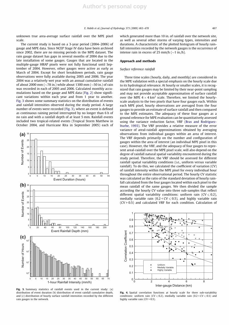
The current study is based on a 3-year period (2004–2006) ofgauge and MPE data. Since NCEP Stage IV data have been archivedsince 2002, there are no missing periods in the MPE dataset. Therain gauge dataset has gaps in several months of 2004 due to thelate installation of some gauges. Gauges that are located in themultiple-gauge HRAP pixels were not fully functional until Sep-tember of 2004. However, other gauges were active as early asMarch of 2004. Except for short breakdown periods, rain gaugeobservations were fully available during 2005 and 2006. The year2004 was a relatively wet year with an annual cumulative rainfallof about 2000 mm (�78 in.) while about 1300 mm (�50 in.) of rainwas recorded in each of 2005 and 2006. Calculated monthly accu-mulations based on the gauge and MPE data (Fig. 2) show signifi-cant variations within each year and from 1 year to another.Fig. 3 shows some summary statistics on the distribution of eventsand rainfall intensities observed during the study period. A largenumber of events were recorded (Fig. 3), where an event is definedas continuous raining period interrupted by no longer than 6 h ofno rain and with a rainfall depth of at least 5 mm. Rainfall eventsincluded two tropical-related events (Tropical Storm Matthew inOctober 2004, and Hurricane Rita in September 2005) each of

which generated more than 10 in. of rainfall over the network site,as well as several other storms of varying types, intensities anddurations. A characteristic of the plotted histogram of hourly rain-fall intensities recorded by the network gauges is the occurrence ofintense rain in excess of 25 mm/h (�1 in./h).

Approach and methods

Surface reference rainfall

Three time scales (hourly, daily, and monthly) are considered inthe MPE validation with a special emphasis on the hourly scale dueto its hydrological relevance. At hourly or smaller scales, it is recog-nized that rain gauges may be limited by their near-point samplingand may not provide acceptable approximation of surface rainfallover the MPE 4 � 4 km2 scale. Therefore, we limited the hourly-scale analysis to the two pixels that have four gauges each. Withineach MPE pixel, hourly observations are averaged from the fourgauges to provide an estimate of surface rainfall and then comparedto the MPE estimates. The adequacy of these four gauges as aground reference for MPE evaluation can be quantitatively assessedusing the variance reduction factor, VRF (Bras and Rodriguez-Iturbe, 1993). The VRF provides a relative measure of the errorvariance of areal-rainfall approximations obtained by averagingobservations from individual gauges within an area of interest.The VRF depends primarily on the number and configuration ofgauges within the area of interest (an individual MPE pixel in thiscase). However, the VRF, and the adequacy of four gauges to repre-sent areal-rainfall over the MPE pixel scale, will also depend on thedegree of rainfall natural spatial variability encountered during thestudy period. Therefore, the VRF should be assessed for differentrainfall spatial variability conditions (i.e., uniform versus variablerainfall). To do this, we calculated the coefficient of variation (CV)of rainfall intensity within the MPE pixel for every individual hourthroughout the entire observational period. The hourly CV statisticwas calculated as the ratio of the standard deviation of hourly rain-fall calculated from the four gauges located within each pixel to themean rainfall of the same gauges. We then divided the sampleaccording the hourly CV value into three sub-samples that reflectdifferent spatial variability conditions: uniform rain (CV 6 0.2),medially variable rain (0.2 < CV 6 0.5), and highly variable rain(CV > 0.5) and calculated VRF for each condition. Calculation of

1-hour Rainfall Intensity (mm/h)

Num

ber o

f Hou

rs

0 5 10 15 20 25 30 35 40 45 50 55 60 65 70

100

101

102

103

Event Duration (hours)

Num

ber o

f Eve

nts

0 5 10 15 20 25 30 35 40 45 50 550

5

10

15

20

25

30

Event Rainfall Depth (mm)

Num

ber o

f Eve

nts

0 20 40 60 80 100 120 140 160 180 2000

5

10

15

20

25

30

35

(a)

(b)

(c)

Fig. 3. Summary statistics of rainfall events used in the current study: (a)distribution of event duration (b) distribution of event rainfall cumulative depth,and (c) distribution of hourly surface rainfall intensities recorded by the differentrain gauges in the network.

+

+

++ ++

+ + +++ ++

++

++

++

+ ++ +++

+

++

+

++

++

++

++++ ++ +

++ +++ +

+ ++ ++

+++ +

+++

+

+++

+

+

+ ++

++ ++

+ +

++ +

Inter-gauge Distance (km)

Cor

rela

tion

Coe

ffici

ent

0 2 4 6 80

0.1

0.2

0.3

0.4

0.5

0.6

0.7

0.8

0.9

1

UniformMedially VariableHighly Variable

+

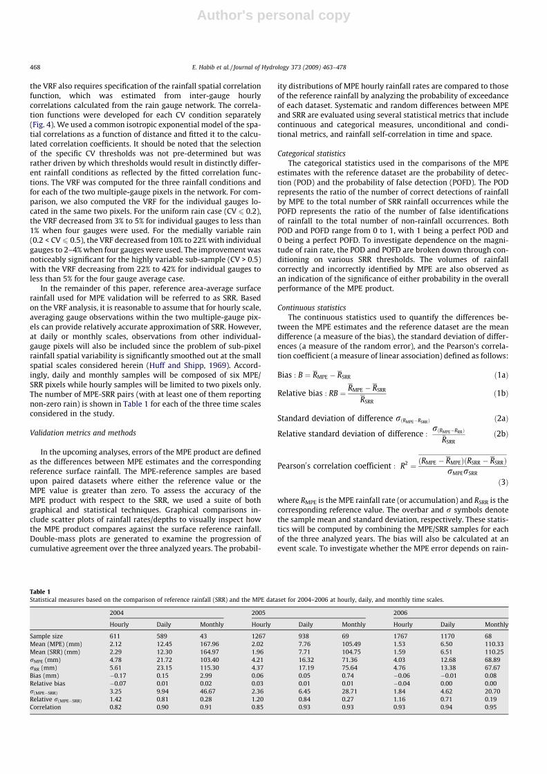
Fig. 4. Spatial correlation functions at hourly scale for three sub-variabilityconditions: uniform rain (CV 6 0.2), medially variable rain (0.2 < CV 6 0.5) andhighly variable rain (CV > 0.5).



the VRF also requires specification of the rainfall spatial correlationfunction, which was estimated from inter-gauge hourlycorrelations calculated from the rain gauge network. The correla-tion functions were developed for each CV condition separately(Fig. 4). We used a common isotropic exponential model of the spa-tial correlations as a function of distance and fitted it to the calcu-lated correlation coefficients. It should be noted that the selectionof the specific CV thresholds was not pre-determined but wasrather driven by which thresholds would result in distinctly differ-ent rainfall conditions as reflected by the fitted correlation func-tions. The VRF was computed for the three rainfall conditions andfor each of the two multiple-gauge pixels in the network. For com-parison, we also computed the VRF for the individual gauges lo-cated in the same two pixels. For the uniform rain case (CV 6 0.2),the VRF decreased from 3% to 5% for individual gauges to less than1% when four gauges were used. For the medially variable rain(0.2 < CV 6 0.5), the VRF decreased from 10% to 22% with individualgauges to 2–4% when four gauges were used. The improvement wasnoticeably significant for the highly variable sub-sample (CV > 0.5)with the VRF decreasing from 22% to 42% for individual gauges toless than 5% for the four gauge average case.

In the remainder of this paper, reference area-average surfacerainfall used for MPE validation will be referred to as SRR. Basedon the VRF analysis, it is reasonable to assume that for hourly scale,averaging gauge observations within the two multiple-gauge pix-els can provide relatively accurate approximation of SRR. However,at daily or monthly scales, observations from other individual-gauge pixels will also be included since the problem of sub-pixelrainfall spatial variability is significantly smoothed out at the smallspatial scales considered herein (Huff and Shipp, 1969). Accord-ingly, daily and monthly samples will be composed of six MPE/SRR pixels while hourly samples will be limited to two pixels only.The number of MPE-SRR pairs (with at least one of them reportingnon-zero rain) is shown in Table 1 for each of the three time scalesconsidered in the study.

Validation metrics and methods

In the upcoming analyses, errors of the MPE product are definedas the differences between MPE estimates and the correspondingreference surface rainfall. The MPE-reference samples are basedupon paired datasets where either the reference value or theMPE value is greater than zero. To assess the accuracy of theMPE product with respect to the SRR, we used a suite of bothgraphical and statistical techniques. Graphical comparisons in-clude scatter plots of rainfall rates/depths to visually inspect howthe MPE product compares against the surface reference rainfall.Double-mass plots are generated to examine the progression ofcumulative agreement over the three analyzed years. The probabil-

ity distributions of MPE hourly rainfall rates are compared to thoseof the reference rainfall by analyzing the probability of exceedanceof each dataset. Systematic and random differences between MPEand SRR are evaluated using several statistical metrics that includecontinuous and categorical measures, unconditional and condi-tional metrics, and rainfall self-correlation in time and space.

Categorical statisticsThe categorical statistics used in the comparisons of the MPE

estimates with the reference dataset are the probability of detec-tion (POD) and the probability of false detection (POFD). The PODrepresents the ratio of the number of correct detections of rainfallby MPE to the total number of SRR rainfall occurrences while thePOFD represents the ratio of the number of false identificationsof rainfall to the total number of non-rainfall occurrences. BothPOD and POFD range from 0 to 1, with 1 being a perfect POD and0 being a perfect POFD. To investigate dependence on the magni-tude of rain rate, the POD and POFD are broken down through con-ditioning on various SRR thresholds. The volumes of rainfallcorrectly and incorrectly identified by MPE are also observed asan indication of the significance of either probability in the overallperformance of the MPE product.

Continuous statisticsThe continuous statistics used to quantify the differences be-

tween the MPE estimates and the reference dataset are the meandifference (a measure of the bias), the standard deviation of differ-ences (a measure of the random error), and the Pearson’s correla-tion coefficient (a measure of linear association) defined as follows:

Bias : B ¼ RMPE � RSRR ð1aÞ

Relative bias : RB ¼ RMPE � RSRR

RSRRð1bÞ

Standard deviation of difference rðRMPE�RSRRÞ ð2aÞ

Relative standard deviation of difference :rðRMPE�RRRÞ

�RSRRð2bÞ

Pearson0s correlation coefficient : R2 ¼ ðRMPE � RMPEÞðRSRR � RSRRÞrMPErSRR

ð3Þ

where RMPE is the MPE rainfall rate (or accumulation) and RSRR is thecorresponding reference value. The overbar and r symbols denotethe sample mean and standard deviation, respectively. These statis-tics will be computed by combining the MPE/SRR samples for eachof the three analyzed years. The bias will also be calculated at anevent scale. To investigate whether the MPE error depends on rain-

Table 1Statistical measures based on the comparison of reference rainfall (SRR) and the MPE dataset for 2004–2006 at hourly, daily, and monthly time scales.

2004 2005 2006

Hourly Daily Monthly Hourly Daily Monthly Hourly Daily Monthly

Sample size 611 589 43 1267 938 69 1767 1170 68Mean (MPE) (mm) 2.12 12.45 167.96 2.02 7.76 105.49 1.53 6.50 110.33Mean (SRR) (mm) 2.29 12.30 164.97 1.96 7.71 104.75 1.59 6.51 110.25rMPE (mm) 4.78 21.72 103.40 4.21 16.32 71.36 4.03 12.68 68.89rRR (mm) 5.61 23.15 115.30 4.37 17.19 75.64 4.76 13.38 67.67Bias (mm) �0.17 0.15 2.99 0.06 0.05 0.74 �0.06 �0.01 0.08Relative bias �0.07 0.01 0.02 0.03 0.01 0.01 �0.04 0.00 0.00r(MPE�SRR) 3.25 9.94 46.67 2.36 6.45 28.71 1.84 4.62 20.70Relative r(MPE�SRR) 1.42 0.81 0.28 1.20 0.84 0.27 1.16 0.71 0.19Correlation 0.82 0.90 0.91 0.85 0.93 0.93 0.93 0.94 0.95



fall magnitudes, the statistical metrics will also be analyzed by con-ditioning on various ranges of the reference rainfall.

Self-correlation statisticsThe validation metrics described so far are based on comparisons

of individual MPE pixel estimates to the corresponding SRR valuesover the same pixel. Another approach focuses on the analysis ofthe underlying structure of the rainfall fields (e.g., Gebremichaeland Krajewski, 2004; Germann and Joss, 2001; Harris et al., 2001;Ebert and McBride, 2000; Marzban and Sandgathe, 2009). Such ananalysis (e.g., variograms or correlation functions) provides insightinto how the MPE product can reproduce the spatial and temporalorganization of the surface rainfall. A full examination of this aspectof the validation process across a wide range of scales is not possiblein the current study due to the limited spatial extent of the referencenetwork, which covers only few MPE pixels. Therefore, we examinethe self-correlation present in the reference and MPE datasets by cal-culating the spatial auto-correlation at one lag only (4-km). The tem-poral auto-correlation can be calculated at several lags starting from1 h.

Error decompositionTo gain more insight on the source of MPE errors, the overall

bias between the MPE estimates and the reference rainfall can befurther decomposed as follows. The bias calculated using Eq. (1)is based on aggregation of differences in rainfall volume over theentire sample and does not provide information on the source ofsuch differences. Therefore, it is desirable to break down the totalbias into three components consisting of the bias associated withsuccessful detections (hits), bias due to rainfall misses, and biasdue to false detections:

Hit bias ðHBÞ ¼XðRMPEðRMPE > 0 & RSRR > 0Þ

� RSRRðRMPE > 0 & RSRR > 0ÞÞ ð4Þ

Missed-rain bias ðMBÞ ¼X

RSRRðRMPE ¼ 0 & RSRR > 0Þ ð5Þ

False-rain bias ðFBÞ ¼X

RMPEðRMPE > 0 & RSRR ¼ 0Þ ð6Þ

Such decomposition can distinguish among the three possiblebias sources, whose values can be cancelled by opposite signs ifthe total bias is only evaluated. The summation of these three com-ponents adds up to the total bias ðTB ¼

PðRMPE � RSRRÞÞ. The pro-

portion of total bias attributed to each bias source can bedescribed by the ratio of the particular bias component to the totalbias (e.g., HB/TB, MB/TB, and FB/TB), with the three ratios adding upto 1.

Results and discussion

We start by showing some graphical comparisons between theMPE product and the reference rainfall dataset. As shown earlier,monthly comparisons of MPE versus the reference rainfall dataset(Fig. 2), indicate that the MPE estimates were able to capture theoverall monthly trends and magnitudes. Cumulative rainfall ob-served by the MPE and the reference dataset SRR as a function oftime are shown in the form of double-mass curves (Fig. 5). Theseplots are produced by accumulating MPE and surface rainfall overone of the four-gauge pixels. Ideal agreement on double-masscurves is identified when the plotted curve is parallel to the 1:1line; any deviation from this direction is an indication of cumula-tive drift (either overestimation or underestimation) by the MPEestimates in comparison to the reference rainfall. In 2004, signsof such drifts are evident especially in August, early October, lateNovember and December. The comparison is relatively better in2005 and 2006 where approximate equality between MPE and sur-

Augu

st

Sept

embe

r

Oct

ober

Nov

embe

r

Dec

embe

r

MPE

Cum

ulat

ive

Rai

nfal

l(m

m)

0 100 200 300 400 500 600 7000

100

200

300

400

500

600

700M

ay

Mar

chAp

ril

Febr

uary

June

July

Augu

st Sept

embe

r

Nov

embe

r

Dec

embe

r

MPE

Cum

ulat

ive

Rai

nfal

l(m

m)

0 200 400 600 800 1000 12000

200

400

600

800

1000

1200

Febr

uary

April

May

June

July

Augu

st

Sept

embe

r

Oct

ober

Nov

embe

r

Dec

embe

r

SRR Cumulative Rainfall (mm)

MPE

Cum

ulat

ive

Rai

nfal

l(m

m)

0 200 400 600 800 1000 1200 14000

200

400

600

800

1000

1200

1400

2005

2004

2006

Fig. 5. Double mass curves showing the cumulative rainfall of the MPE and SRR as afunction of time for 2004, 2005, and 2006 using data from one of the 4-gauge MPEpixels. Vertical lines indicate the beginning of each month.



face rainfall is noticed in several months. Staircase-like features,which indicate detection problems, are also observed (e.g., duringNovember months in 2004 and 2005).

Analysis of rainfall distributions

Distribution-based comparisons can be made by examiningscatter plots of the MPE estimates versus the reference values(Fig. 6). These graphs are generated by pooling data pairs fromall relevant pixels (2 pixels for the hourly scale and 6 pixels forthe daily and monthly scales). Significant scatter exists betweenthe MPE estimates and the corresponding reference values at thehourly scale where differences as large as 15–20 mm/h are notuncommon. Several instances of failed and false detection byMPE are observed. As expected, the scatter is reduced as the MPEestimates are accumulated to longer time scales such as dailyand monthly. However, significant differences are still observed

at such scales (up to 20–25 mm/day at the daily scale and up to50 mm/month at the monthly scale). An improvement over timeis apparent in the relatively reduced scatter in 2006 compared to2004 and 2005.

To further examine the distributional agreement, the marginaldistributions of the MPE estimates and the surface reference rain-fall were analyzed by examining the probability of exceedance ofeach dataset (Fig. 7). The probability of exceedance is definedand calculated as the probability that an estimate exceeds a certainthreshold. This analysis is relevant from a hydrologic predictionpoint of view since it examines the exceedance of extreme rainfallthresholds, which are usually responsible for triggering flash floodsor other extreme natural events. For this reason and sample sizelimitations, results from the hourly and daily scales only are pre-sented. Consider the extreme tail of the distributions, which canbe loosely defined by the hourly rain rate exceeding 8–10 mm/h(�5–10% hourly exceedance probability) and the daily rainfall

Fig. 6. Scatter plots of MPE versus SRR for 2004–2006 at hourly, daily, and monthly time scales.



depth exceeding 20–30 mm (�5–10% daily exceedance probabil-ity). A close agreement between the tails of the two distributionsis clear (especially in 2005 and 2006), which indicates the abilityof MPE estimates to represent the occurrences of extreme rainfallvalues. The two distributions deviate at the extreme tail (1%exceedance or lower) where the MPE distribution shows less num-ber of occurrences of such extreme intensities. However, it shouldbe noted that the estimation of the most extreme tail of the distri-butions may be subject to sampling effects.

Analysis of MPE Bias

The overall total bias between the MPE estimates and the refer-ence rain is quantified by calculating the difference between theirarithmetic means over every year and is expressed in absolute andrelative units (Eqs. (1a) and (1b)); Table 1. When aggregated overthe full sample of each year, the MPE estimates have relativelysmall bias values. These results agree with earlier MPE evaluationstudies which reported low bias levels of the MPE products(e.g., Westcott et al., 2008; Wang et al., 2008). In addition to aggre-gating the bias over each year, we also assessed the bias on anevent scale (Fig. 8), where an event is defined as continuous rainingperiod interrupted by no longer than 6 h of no rain and with a rain-fall depth of at least 5 mm. Overall, about 50% of the events have abias within ±25%, 90% of them have a bias within ±50%, and only10% of the events have a bias exceeding 50% with some as highas 100%. The histogram of event-scale bias indicates a skewed dis-tribution with 65% of events having a negative underestimationbias. Events with high average rain rate (>8 mm/h) are mostlycharacterized with negative bias.

As described earlier, the total bias consists of three compo-nents; hit bias, missed-rain bias, and false-rain bias, the values ofwhich may cancel each other when added up to form the total bias.The three bias components were calculated at the hourly scale and

are shown for the two four-gauge pixels (Fig. 9); note that thesevolumes are combined totals from the two individual pixels. Thepercentages shown in the figure represent bias values relative tothe total rainfall depth. It is clear that the three bias components

100 101 10210-3

10-2

10-1

2006

100 101 10210-3

10-2

10-1

2005

Rainfall (mm)

Prob

.ofE

xcee

danc

eof

Dai

lyR

ainf

all

100 101 10210-3

10-2

10-1

Rainfall (mm)100 101 102

10-3

10-2

10-1

Rainfall (mm)100 101 102

10-3

10-2

10-1

Prob

.ofE

xcee

danc

eof

Hou

rlyR

ainf

all

100 101 10210-3

10-2

10-1

SRRMPE

2004

Fig. 7. Probability of exceedance plots of SRR and MPE at hourly (upper panels) and daily (lower panels) time scales.

Relative Bias

Num

bero

fEve

nts

-1 -0.8 -0.6 -0.4 -0.2 0 0.2 0.4 0.6 0.8 10

10

20

30

40

50

Event Mean Rain Rate (mm/h)

Rel

ativ

eBi

as

0 2 4 6 8 10 12 14 16 18-1

0

1

2

3

(a)

(b)

Fig. 8. (a) Distribution of the event-scale bias of the MPE estimates for all rainfallevents in 2004–2006. (b) Event-relative bias as a function of the event mean rainrate.



have comparable magnitudes (�2% to 8%) to each other and to theoverall bias. While the hit-bias explains a significant portion of theoverall MPE bias, both the false rain and the missed rain have com-parable contributions. It is also interesting to observe that the va-lue of each of the three bias components can be cancelled ordiminished by the other components due to their respective signs;therefore, examining only the total overall bias can be rathermisleading.

To examine whether the MPE bias is dependent on the rain ratemagnitude, the full sample was divided into sub-samples based ondifferent ranges of the reference rain rate and the conditional biaswas calculated for every range (Fig. 10). The relative bias is calcu-lated by normalizing with the mean rain rate of each range. Toavoid deterioration of the sample size, the conditioning was doneafter pooling together data from the 3 years. It is clear that theMPE bias depends on the magnitude of the rain rate. The bias tendsto be positive for the lower range of reference rates and decreasesgradually to become negative for higher rates. While the uncondi-tional bias was in the range of 3–7%, the conditional bias has ratherhigh levels (60–90%) at small intensities (<0.5 mm/h) and de-creases to about �20% at large rainfall rates (>10 mm/h). This over-all behavior of the conditional bias, which is consistent across thethree analyzed years, indicates that the MPE estimates tend tooverestimate small rain rates and underestimate large rain rates.Similar observations of this behavior were also reported in otherMPE evaluation studies (e.g., Westcott et al., 2008).

Analysis of MPE detection

To further characterize the detection capability of the MPEproduct, we examine two probabilities: probability of detection(POD), and probability of false detection (POFD); Fig. 11. To exam-ine the significance of detection limitations in MPE estimates, wealso kept track of the volume of rain that is either missed due tolack of detection (POD < 1) or falsely detected (i.e., POFD > 0). Thisanalysis is reported for the hourly scale only. Consider first the PODresults. Conditioned on SRR larger than zero, the MPE estimatesshow low to medium POD values (0.5–0.6). The undetected surfacerainfall exceeded 1 mm/h for less than 0.6% of the time (largestvalue is 6.5 mm/h). When conditioned on surface rain rates largerthan a certain threshold, the POD increases which indicates that

the rather low POD values are caused by lack of detection of smallrainfall intensities (less than 0.13 mm/h). The POD increases toabout 0.9 when conditioning on surface rain rates larger than0.13 mm/h. As shown earlier in the bias decomposition results,the volume missed due to lack of detection is smaller than 5% ofthe total rainfall volume. The POD continues to improve with theincrease of the surface threshold rain rate and reaches 0.9 andhigher when SRR is larger than 1 mm/h. The volume of missed raindiminishes and approaches zero at a threshold of 7 mm/h. Resultson the POFD (Fig. 11) show that false detection of rainfall by MPEoccurs less than 2% of the time. This translates into a falsely de-tected volume of rainfall of 5% or lower. Falsely detected intensitieshad a maximum of 8 mm/h and exceeded 1 mm/h for less than 1%of the time. Similar to the POD, the PODF values decline rapidlywith the increase of the rainfall threshold which indicates thatmost false detection cases were associated with low MPE intensi-ties. It should be noted that POD and PODF values, especially atlow thresholds, are sensitive to differences in the minimum detect-able rainfall by MPE and SRR. The minimum SRR non-zero value iscontrolled by the average of observations from individual raingauges, each of which has a detectable threshold of 0.254 mm/h.While the first stage of the MPE product (Stage I or DPA) has athreshold of 0.25 mm/h, the final MPE product can have rainfallhourly values that are lower than 0.25 mm/h (over the area of thisstudy, the minimum MPE non-zero rainfall amount was found tobe 0.13 mm/h). This particular value is not enforced by the MPEalgorithm; instead, it is possibly a result of various data processingeffects such as spatial interpolation between a zero gauge reportand a nonzero radar report, bias adjustment of radar data, or mosa-icking of zero and no-zero regional radar analyses into the nationalStage IV product (personal correspondence with David Kitzmiller,NWS, and Ying Lin, NCEP).

Analysis of agreement and disagreement statistics

The linear association between MPE and the reference rainfall isassessed using the Pearson’s correlation coefficient (Table 1). Over-all, the MPE hourly estimates show strong correlation values(around 0.8 for 2004 and 2005 and above 0.9 for 2006), which re-flects a reasonable skill for the MPE product in reproducing thetemporal fluctuations of the reference rainfall. The correlation ex-

Rai

nfal

lDep

th(m

m)

-200

-150

-100

-50

0

50

100

150

200

Hit BiasMissed RainFalse RainTotal Bias

2004 2005 2006

-8.4%

-4.4%

5.6%

-7.2%

2.7%

-2.6%

3.2% 3.2%

-5.2%

-2.7%

4.3%

-3.6%

Fig. 9. Decomposition of the total bias of the MPE into its three components, hit bias, missed rain, and false rain for each year. The percentage shown above each bar indicatesthe ratio of the bias component to the total annual rainfall amount.



ceeds 0.9 when the MPE is accumulated to daily and monthlyscales. Similar to the conditional bias, the correlation level dependson the magnitude of surface rainfall intensity (Fig. 10). Very lowcorrelation values are reported for the small to medium rainfallintensities, which indicates a poor association between the MPEestimates and the reference rainfall at such intensities but alsomay be partly attributed to data quantization and limited resolu-tions. High correlations are obtained only for large rainfall intensi-ties (>10 mm/h), which reflects the ability of MPE estimates tobetter track surface rainfall during the intense part of the storms.However, such high correlation levels might be artificially inflatedto some extent due to the sensitivity of the Pearson’s correlationstatistic to extreme values.

Now we turn to statistics that focus on assessing disagreementbetween MPE and reference rainfall using the standard deviation ofdifferences between MPE and SRR hourly intensities. The standarddeviation of differences is calculated unconditionally Table 1 for

each year and conditionally on different intervals of SRR after com-bining data from the 3 years (Fig. 10). The results are presented inabsolute units (mm/h) and also as a ratio relative to the mean rain-fall rate of each SRR interval. The unconditional standard deviationof differences exceeds 100% in each of the 3 years. When condi-tioned on the magnitude of rainfall intensity, the relative standarddeviation attains relatively high values (200–400%) for small inten-sities (<0.5 mm/h), remains around 100% for intermediate intensi-ties (0.5–2 mm/h) and decreases to less than 50% for large rainfallintensities (>5–10 mm/h).

Rainfall self-correlation structure

We now examine how the MPE product can reproduce theunderlying spatial and temporal organization present in the sur-face rainfall. Consider first the spatial auto-correlation. Ideally,one should establish correlation functions or variograms from thetwo datasets at various spatial lags. However, based on the gaugenetwork spatial setup, estimation of surface rainfall is availableonly over the two 4-gauge pixels. Therefore, we limited the autospatial correlation analysis to one lag only of 4-km, which is theseparation distance between these two neighboring pixels. Corre-lation coefficients between hourly rainfall intensities at the twopixels were calculated for both the reference rainfall and theMPE product. The results represent correlation coefficients ofhourly intensities stratified by the month (Fig. 12). The overall cor-relation trends of the MPE are very similar to those of the referencerainfall, especially during cold months. The agreement is still rea-sonable during warm months (except June) with MPE having over-all lower self-correlation levels, which is likely due to thedominance of highly variable localized storms during this time ofthe year. Unlike the spatial correlation, the temporalauto-correlation can be calculated for various time lags; however,results for 1-h lag only are presented (Fig. 12) since the correlationbecomes practically negligible for longer lags. As expected, tempo-ral auto-correlations are generally low, but it is interesting to seethat the MPE data produces similar temporal 1-h self-correlationvalues to those of the surface rainfall.

Effect of pixel sub-variability and gauge sampling errors on MPEevaluation

In most studies that are concerned with evaluation of radar-based rainfall products, single-gauge measurements are usuallyused as the surface rainfall reference. As discussed earlier, thenear-point sampling of a single gauge and its limited representa-tion of area-average rainfall over the size of a 4 � 4 km2 MPE pixelcan contaminate the information sought on actual MPE estimatederrors. The experimental setup available in this study makes it pos-sible to further investigate this issue and provide a quantitativeassessment of such contamination. To do this, we follow a simpledata-based approach and recalculate the MPE error assuming sin-gle-gauge observations as the reference rainfall. Then, we comparethe results to those obtained earlier when average observationsfrom four gauges within one pixel were used as the reference rain-fall. To be consistent, the single-gauge analysis was based only onindividual gauges from those located within the two 4-gaugepixels. The impact of using single-gauge observations as a refer-ence is expected to depend on how variable rainfall is over thescale of an MPE pixel. Therefore, we divided the data into the samethree sub-samples used earlier (Section ‘‘Surface reference rain-fall”) which represent uniform rain (CV 6 0.2), medially variablerain (0.2 < CV 6 0.5) and highly variable rain (CV > 0.5). Statisticsof the MPE performance using both sets of reference rainfall (singlegauge and average of gauges) are compared in terms of bias, stan-dard deviation of differences and the correlation coefficient

Rel

ativ

eBi

as

-0.4

-0.2

0

0.2

0.4

0.6

0.8

1

1.2

1.4

200420052006

0.13 - 0

.30

0.30 - 0

.50

0.50 - 0

.80

0.80 - 1

.25

1.25 - 2

.0

2.0- 4

.0

4.0- 7

.0

7.0- 1

0.0

> 10.0

-2

-1

0

1

2

3

4

5

6

7

8

0.13 - 0

.30

0.30 - 0

.50

0.50 - 0

.80

0.80 - 1

.25

1.25 - 2

.0

2.0- 4

.0

4.0- 7

.0

7.0- 1

0.0

> 10.0

Rel

ativ

eσ

(MPE

-SR

R)

Interval of SRR Rainfall Rate (mm/h)

Cor

rela

tion

Coe

ffici

ent

-0.4

-0.2

0

0.2

0.4

0.6

0.8

1

0.13 - 0

.30

0.30 - 0

.50

0.50 - 0

.80

0.80 - 1

.25

1.25 - 2

.0

2.0- 4

.0

4.0- 7

.0

7.0- 1

0.0

> 10.0

Fig. 10. Statistical performance measures of MPE versus SRR conditioned onvarious ranges of SRR.



(Table 2). As expected, the MPE bias is not affected since individualgauges can usually provide reasonable approximation of long-termrainfall accumulations. However, compared to the average-gaugecase, the single-gauge performance statistics shows a worse thanactual MPE performance as reported in the standard deviation ofdifferences and in the correlation coefficient. These two statisticsreport larger differences between the single-gauge and average-gauge analysis within the samples that are characterized withhigher degrees of sub-pixel variability. For the highly variablesub-sample, the change in the standard deviation of the differencesincreased to almost 40% and the decrease in the correlationcoefficient became close to 20%. Even with the case of medium var-iability, the performance statistics still show significant differences(about 20% increase in the standard deviation and 6% decrease inthe correlation). These results indicate that relying on observationsof a single gauge within an MPE pixel will lead to an understate-ment of the MPE performance caused by inaccuracy that is not to-tally attributable to the MPE estimates.

More insight into the effect of the lack of representativeness ofsingle gauges as a surface rainfall reference on the MPE evaluationcan be gained through the following formulation:

ðRMPE � RGÞ ¼ ðRMPE � RSRRÞ þ ðRSRR � RGÞ ð7Þ

This formulation is based on the concept of error separation(first introduced by Ciach and Krajewski, 1999a,b) in which the to-tal difference between MPE estimates and individual gauge obser-vations (RG) can be decomposed into two components. The firstcomponent (first term on RHS of (6)) is the difference betweenMPE and the reference surface rainfall (RRR) obtained by averaging

Threshold (mm/h)

POFD

(%)

Fals

ely

Det

ecte

dR

ain

Dep

th(%

ofto

talr

ain)

0 2 4 6 8 100

1

2

0

0.5

1

1.5

2

2.5

3

3.5

4

4.5

5

POFDFalse rain

Threshold (mm/h)

POD

(%)

Mis

sed

Rai

nD

epth

(%of

tota

lrai

n)

0 2 4 6 80

20

40

60

80

100

0

0.5

1

1.5

2

2.5

3

PODMissed rain

(a)

(b)

Fig. 11. (a) Probability of detection (POD) of MPE conditioned on various SRR thresholds (left y-axis) and the corresponding percentage of missed rain (right y-axis). (b)Probability of false detection (POFD) of MPE condition on various SRR thresholds (left y-axis) and the corresponding percentage of falsely detected rain (right y-axis).

Month

Tem

pora

lAut

o-co

rrela

tion

1 2 3 4 5 6 7 8 9 10 11 12-0.2

0

0.2

0.4

0.6

Month

Spat

ialA

uto-

corre

latio

n

1 2 3 4 5 6 7 8 9 10 11 120.5

0.6

0.7

0.8

0.9

1

SRRMPE

(a)

(b)

Fig. 12. Spatial (a) and temporal (b) auto-correlation of hourly rainfall for MPE andSRR stratified by the month.



observations from the four gauges within each pixel, and repre-sents the actual MPE error. The second component (second termon RHS of (6)) is the difference between the gauge and the refer-ence rainfall and represents the gauge error due to lack of arealrepresentativeness. In typical validation studies, information onRRR is usually unavailable and the ðRMPE � RGÞ differences are as-sumed as surrogate for the actual MPE error ðRMPE � RSRRÞ:

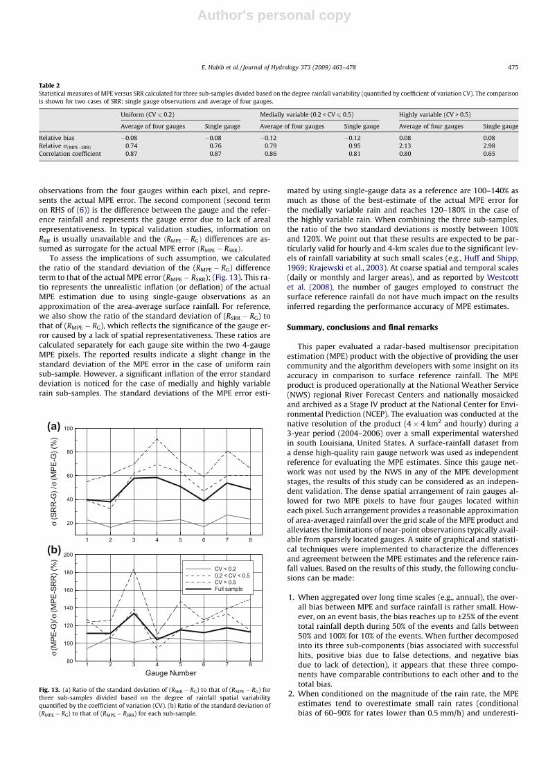
To assess the implications of such assumption, we calculatedthe ratio of the standard deviation of the (RMPE � RG) differenceterm to that of the actual MPE error (RMPE � RSRR); (Fig. 13). This ra-tio represents the unrealistic inflation (or deflation) of the actualMPE estimation due to using single-gauge observations as anapproximation of the area-average surface rainfall. For reference,we also show the ratio of the standard deviation of (RSRR � RG) tothat of (RMPE � RG), which reflects the significance of the gauge er-ror caused by a lack of spatial representativeness. These ratios arecalculated separately for each gauge site within the two 4-gaugeMPE pixels. The reported results indicate a slight change in thestandard deviation of the MPE error in the case of uniform rainsub-sample. However, a significant inflation of the error standarddeviation is noticed for the case of medially and highly variablerain sub-samples. The standard deviations of the MPE error esti-

mated by using single-gauge data as a reference are 100–140% asmuch as those of the best-estimate of the actual MPE error forthe medially variable rain and reaches 120–180% in the case ofthe highly variable rain. When combining the three sub-samples,the ratio of the two standard deviations is mostly between 100%and 120%. We point out that these results are expected to be par-ticularly valid for hourly and 4-km scales due to the significant lev-els of rainfall variability at such small scales (e.g., Huff and Shipp,1969; Krajewski et al., 2003). At coarse spatial and temporal scales(daily or monthly and larger areas), and as reported by Westcottet al. (2008), the number of gauges employed to construct thesurface reference rainfall do not have much impact on the resultsinferred regarding the performance accuracy of MPE estimates.

Summary, conclusions and final remarks

This paper evaluated a radar-based multisensor precipitationestimation (MPE) product with the objective of providing the usercommunity and the algorithm developers with some insight on itsaccuracy in comparison to surface reference rainfall. The MPEproduct is produced operationally at the National Weather Service(NWS) regional River Forecast Centers and nationally mosaickedand archived as a Stage IV product at the National Center for Envi-ronmental Prediction (NCEP). The evaluation was conducted at thenative resolution of the product (4 � 4 km2 and hourly) during a3-year period (2004–2006) over a small experimental watershedin south Louisiana, United States. A surface-rainfall dataset froma dense high-quality rain gauge network was used as independentreference for evaluating the MPE estimates. Since this gauge net-work was not used by the NWS in any of the MPE developmentstages, the results of this study can be considered as an indepen-dent validation. The dense spatial arrangement of rain gauges al-lowed for two MPE pixels to have four gauges located withineach pixel. Such arrangement provides a reasonable approximationof area-averaged rainfall over the grid scale of the MPE product andalleviates the limitations of near-point observations typically avail-able from sparsely located gauges. A suite of graphical and statisti-cal techniques were implemented to characterize the differencesand agreement between the MPE estimates and the reference rain-fall values. Based on the results of this study, the following conclu-sions can be made:

1. When aggregated over long time scales (e.g., annual), the over-all bias between MPE and surface rainfall is rather small. How-ever, on an event basis, the bias reaches up to ±25% of the eventtotal rainfall depth during 50% of the events and falls between50% and 100% for 10% of the events. When further decomposedinto its three sub-components (bias associated with successfulhits, positive bias due to false detections, and negative biasdue to lack of detection), it appears that these three compo-nents have comparable contributions to each other and to thetotal bias.

2. When conditioned on the magnitude of the rain rate, the MPEestimates tend to overestimate small rain rates (conditionalbias of 60–90% for rates lower than 0.5 mm/h) and underesti-

Table 2Statistical measures of MPE versus SRR calculated for three sub-samples divided based on the degree rainfall variability (quantified by coefficient of variation CV). The comparisonis shown for two cases of SRR: single gauge observations and average of four gauges.

Uniform (CV 6 0.2) Medially variable (0.2 < CV 6 0.5) Highly variable (CV > 0.5)

Average of four gauges Single gauge Average of four gauges Single gauge Average of four gauges Single gauge

Relative bias �0.08 �0.08 �0.12 �0.12 0.08 0.08Relative r(MPE�SRR) 0.74 0.76 0.79 0.95 2.13 2.98Correlation coefficient 0.87 0.87 0.86 0.81 0.80 0.65

1 2 3 4 5 6 7 8

20

40

60

80

100

(SR

R-G

)/σ

σ(M

PE-G

)(%

)

Gauge Number1 2 3 4 5 6 7 880

100

120

140

160

180

200

CV < 0.20.2 < CV < 0.5CV > 0.5Full sample

(MPE

-G)/

σσ

(MPE

-SR

R)(

%)

(a)

(b)

Fig. 13. (a) Ratio of the standard deviation of (RSRR � RG) to that of (RMPE � RG) forthree sub-samples divided based on the degree of rainfall spatial variabilityquantified by the coefficient of variation (CV). (b) Ratio of the standard deviation of(RMPE � RG) to that of (RMPE � RSRR) for each sub-sample.



mate large rain rates (conditional bias of �20% for rates higherthan 10 mm/h). Similarly, the relative standard deviation ofMPE differences from surface rain rates is quite high(200–400% of mean rainfall intensity) for small intensities(<0.5 mm/h), remains around 100% for intermediate intensities(0.5–2 mm/h) and decreases to less than 50% for large rainfallintensities (>5–10 mm/h).

3. Based on the detection analysis, MPE has an overall probabilityof detection of 0.6–0.82; however, most of the undetected rainis in the low range of rain rates (<0.13 mm/h) and a very gooddetection (90% and higher) is achieved for high rain rates. Thepoor detection of small rain rates led to a missed rain amountof no more than 5% of the total rainfall volume. False detectionby MPE occurs less than 3% of the time and is associated withlow rain rates, which indicates that evaporation and rainfall dis-placement by horizontal wind may be a likely reason. To putthese results in a proper perspective, the corresponding PODof a single gauge over the size of an MPE pixel was calculatedand was found to be comparable to that of MPE during highlyand medially uniform rain, but lower by 2% approximately dur-ing highly variable rain. However, it is noted that a single gaugewithin the experimental research network used in this studydoesn’t realistically represent, at least from a data quality per-spective, what one should expect from typical operational raingauges. For such gauges, the POD can be much lower than whatMPE estimates provide.

4. Despite the significant scatter between MPE and surface rain-fall, especially at small intensities, the MPE hourly producthas a good association to surface rainfall rates as reflected bythe high overall correlation (0.82, 0.85, and 0.93 in 2004,2005, and 2006). The correlation well exceeds 0.9 at daily andmonthly scales. However, conditionally the correlation showsvery low values for small to medium rainfall intensities andhigh correlations are obtained only for large rainfall intensities(>10 mm/h).

5. The tail of the MPE probability distribution shows good agree-ment with that of the surface rainfall, which indicates the abil-ity of the MPE product to capture the occurrence of intenserainfall. The MPE product is also successful in reproducing theunderlying spatial and temporal organization of the surfacerainfall as quantified by the spatial and temporalself-correlations. These features are desirable for studies thatrely on radar rainfall products as a driver for modeling varioushydrologic processes.

6. The experimental layout used in this study made it possible toquantify the impact of relying on observations from sparse net-works to validate radar-based rainfall estimates. Using a singlegauge within an MPE pixel as a reference representation of sur-face rainfall resulted in an unrealistic inflation of the actual MPEestimation error by 120–180%. As expected, the most impactwas obtained during highly variable rainfall periods.

7. An overall improvement in the performance of MPE estimateswas reported over the course of the three analyzed years(2004–2006), which was reflected in all of the statistical perfor-mance metrics. The improved performance is likely attributedto factors such as: continuous improvements in the MPE algo-rithm (e.g., mosaicking of overlapping radars, use of climatol-ogy-based effective coverage delineation of individual radars,interactive capabilities for quality control of gauge and radardata) and increased experience by the LMRFC forecasters inusing the MPE algorithm.

8. Compared to previous evaluation studies, the statistics reportedin this study show better performance by the MPE product. Forexample, Young et al. (2008) and Grassotti et al. (2003) showcorrelations in the range of 0.6–0.8 for daily rainfall whilehigher correlations are obtained in the current study (0.8–0.9

for hourly scale and >0.9 for daily scale). We believe that thereason for the observed better performance by MPE is theenhanced quality and accuracy of the rain gauge dataset usedby this study as a validation reference, which ensured thatgauge-related errors are not wrongly assigned to radar estima-tion uncertainties.

In view of the results reported in this paper, the most alarmingfactor about the MPE performance is probably related to the signif-icant levels of bias observed at the event scale. Tracing the sourceof such biases in a post-product validation study is complicated bythe fact that the final MPE product is a result of a multitude of pro-cessing algorithms and procedures that are difficult to trace andisolate. It is known that problems related to hardware calibrationcan introduce systematic errors into radar-rainfall estimates. How-ever, in a comparative analysis versus space-borne radar observa-tions, Anagnostou et al. (2001) found that the KLCH radar sitedoesn’t suffer from any significant calibration problems. MPEBiases could also be the result of using improper Z–R relationships.In principle, the local weather forecast office (WFO) selects a cer-tain Z–R relationship based on season and the prevailing rainfall re-gime and environmental conditions. For example, over the studysite, the WFO in Lake Charles, LA, switches to a tropical Z–R rela-tionship during tropical events. Unfortunately, it was not possiblefor us to trace back which Z–R relationships were used in everyanalyzed event. However, it is also recognized that uncertaintiesin Z–R selection are mitigated by gauge-based bias adjustment pro-cedures. For example, the time-varying mean-field bias correctionapplied within the MPE algorithm is analogous to changing themultiplicative factor, A, in the Z = A � Rb relationship in real-timebased on observed gauge data. Nevertheless, the efficiency of suchbias corrections depends largely on the number and quality of raingauges available to the MPE algorithm in the proximity of studysite. According to the records of the LMRFC, the gauges used bythe MPE algorithm for bias adjustment include one gauge at a dis-tance of �7 km from the study site and four more gauges within10–20 km. We examined the actual event totals of these gaugesand compared them to the corresponding totals from our indepen-dent network and found differences to be comparable in magni-tude to the MPE biases. This indicates some possible data-qualityproblems in the gauges used for MPE bias adjustment. The effectof low-quality gauge data can be significant as shown by Marzenand Fuelberg (2005) who found a six fold increase in the hourlybiases of MPE estimates when the gauge data had not been qualitycontrolled.

Another more plausible source of the MPE biases, especiallyunderestimation, over our study site is due to range-related effects(smith et al., 1996; Hunter, 1996). At a distance of �120 km fromthe closest WSR-88D radar site, the radar beam is at an altitudeof �1.82 km above the validation rain gauge network. At such arange, beam partial filling and overshooting of lower cloud basesand shallower precipitation start to become of a concern. Beamovershooting usually results in low probability of detection; how-ever, lack of detection by MPE over the study site was quite mini-mal and was associated with very light rain except for few hours(undetected intensities exceeding 5 mm/h but less than 7 mm/hwere observed for only 8 h during the entire study period). Relativedegradation of the beam sampling resolution over the study site(beam diameter of 1.85 km, approximately) increases the likeli-hood that rainfall fills only part of the beam and may result inunderestimation of the rainfall intensity due to sample volumeaveraging of the received power. Confirming whether beam over-shooting and spreading is the main source of the observed MPEbiases requires event-by-event diagnosis of radar reflectivity fieldsand other environmental conditions, which is beyond the scope ofthis study. However, the fact that a major number of events were



characterized with a negative bias (i.e., underestimation), espe-cially during heavy rainfall (Figs. 8 and 10) makes range-relatedfactors, especially beam partial filling, the likely source of MPEbiases in this study.

The large MPE biases observed at the event scale are problem-atic especially for hydrologic applications in which accurate pre-diction of rainfall volume is critical. For example, Habib et al.(2008a,b), Vieux and Bedient (2004) and Gourley and Vieux(2005) emphasized the importance of efficient bias removal in ra-dar-based rainfall estimates before accurate model predictions canbe realized. These studies indicated that once the radar bias issuccessfully removed at an event scale, or conditionally, theremaining random errors tend to diminish and get smoothed outby the rainfall-to-runoff transformation. However, this shouldnot de-emphasize the importance of capturing the occurrence ofintense rainfall – an aspect that the MPE data seems to be rathersuccessful with, at least over the domain of this study. With futureenhancement on the horizon for the NWS WSR-88D system andthe MPE algorithm (e.g., higher resolutions in space and time; dualpolarization capabilities; Seo et al., 2005; Ryzhkov et al., 2005), it isanticipated that limitations highlighted in the current study, suchas magnitude-dependent biases and detection problems, will bealleviated so that future MPE products and their utility for floodforecasting and flash flood warnings (Smith et al., 2005) can beenhanced.

This study also emphasizes and reiterates the case made by sev-eral past studies (e.g., Steiner et al., 1999; Krajewski et al., 2003) onthe critical need for experimental surface observation networksthat can provide reliable validation datasets as a prerequisite forthe assessment of current and future remote-sensing based rainfallestimates. In particular, the quantitative results reported in thisstudy indicated that observations from single gauges within anMPE pixel should not be used in validation analysis so that reliableassessment of the product performance can be achieved. This isparticularly important if the validation is performed at small tem-poral scales that are of significance for MPE-driven hydrologicapplications.

Another attribute that is crucially important is the quality ofrain gauge data used in the validation analysis. While this studywas based on high-quality gauges available within an experimen-tal research setup (e.g., regular gauge maintenance and calibration,frequent site visits and downloads, redundancy checks through thedual-gauge setup), other typical gauge networks are usually con-taminated with various gauge-related errors that eventually blurthe validation assessment of any MPE products (Steiner et al.,1999; Marzen and Fuelberg, 2005).

Finally, we point out that the validation analysis reported in thisstudy was mainly driven by product performance evaluation pur-poses. However, information on the statistical characteristics ofthe MPE estimation error (e.g., error distribution, error dependencestructure) are of significant interest for studies that focus on mod-eling and ensemble generation of error fields and their propagationin hydrologic predictions (Ciach et al., 2007; Habib et al., 2008;Villarini et al., 2009; Germann et al., 2006). The setup of the currentrain gauge network, and experimental networks recently devel-oped by other researchers, provide a valuable opportunity for athorough analysis on error characteristics, which is recommendedfor further future studies.

Acknowledgments

This study was funded in part by a subaward with UCAR underthe sponsorship of NOAA/DOC as part of the COMET Outreach Pro-gram, the LaSPACE Graduate Student Research Assistance program,the Louisiana Board of Regents Support Fund Research Competi-tiveness Subprogram, and the NASA/LEQSF(2005–2010)-LaSPACE

contract (NASA grant number NNG05GH22H). The authors alsoacknowledge Ying Lin from NCEP for input regarding the Stage IVdata and Brian R. Nelson and Ali Tokay for their valuable commentsat the early stage of this study. Special thanks to Amy Henschke forassistance in data analysis and producing figures and tables. Valu-able comments from two anonymous reviewers for enhancing thequality of the manuscript are greatly acknowledged.

References

Anagnostou, E.N., Krajewski, W.F., Smith, J., 1999. Uncertainty quantification ofmean-field radar-rainfall estimates. J. Atmos. Ocean. Technol. 16, 206–215.

Anagnostou, E.N., Morales, Carlos A., Dinku, T., 2001. The use of TRMM precipitationradar observations in determining ground radar calibration biases. J. Atmos.Ocean. Technol. 18 (4), 616–628.

Austin, P.M., 1987. Relation between measured radar reflectivity and surfacerainfall. Mon. Wea. Rev. 115, 1053–1070.

Boyles, R., Raman, S., Sims, A., Schwab, S., Horgan, K., Brooks, M., Frazier, A., 2006.Evaluation and applications of NCEP stage II and stage IV gage-corrected radarprecipitation estimates over the Carolinas. In: Preprints, 20th Hydrol. Conf.,Atlanta, GA. Amer. Meteor. Soc. (CD-ROM, 1.1).

Bras, R.L., Rodriguez-Iturbe, I., 1993. Random Functions and Hydrology. Dover, NewYork, USA.

Breidenbach, J.P., Bradberry, J.S., 2001. Multisensor precipitation estimatesproduced by National Weather Service River Forecast Centers for hydrologicapplications. In: Proceedings of the 2001 Georgia Water Resources Conf., March26–27, 2001. Institute of Ecology, University of Georgia, Athens.

Brock, F.V., Crawford, K.C., Elliott, R.L., Cuperus, G.W., Stadler, S.J., Johnson, H.L., Eilts,M.D., 1995. The Oklahoma Mesonet: a technical overview. J. Atmos. Ocean.Technol. 12, 5–19.

Ciach, G.J., Krajewski, W.F., 1999a. Radar-rain gauge comparisons underobservational uncertainties. J. Appl. Meteorol. 38, 519–525.

Ciach, G.J., Krajewski, W.F., 1999b. Radar-rain gauge comparisons underobservational uncertainties. J. Appl. Meteorol. 38, 1519–1525.

Ciach, G.J., Krajewski, W.F., Villarini, G., 2007. Product-error-driven uncertaintymodel for probabilistic quantitative precipitation estimation with NEXRADdata. J. Hydrometeorol. 8 (6), 1325–1347.

Ciach, G., 2003. Local random errors in tipping-bucket rain gauge measurements. J.Atmos. Ocean. Technol. 20 (5), 752–759.

Dyer, J.L., Garza, R., 2004. A comparison of precipitation estimation techniques overLake Okeechobee, Florida. Weather Forecast. 19, 1029–1043.

Ebert, E.E., McBride, J.L., 2000. Verification of precipitation in weather systems:determination of systematic errors. J. Hydrol. 239, 179–202.

Fulton, R.A., Breidenbach, J.P., Seo, D., Miller, D.A., O’Bannon, T., 1998. The WSR-88Drainfall algorithm. Weather Forecast. 13 (2), 380–391.

Fulton, R.A., 2002. Activities to improve WSR-88D radar rainfall estimation in theNational Weather Service. In: 2nd Federal Interagency Hydrologic ModelingConference, Las Vegas, NV, July 28–August 1, 2002.

Gebremichael, M., Krajewski, W.F., 2004. Assessment of the statisticalcharacterization of small-scale rainfall variability from radar: analysis ofTRMM GV data sets. J. Appl. Meteorol. 43 (8), 1180–1199.

Germann, U., Joss, J., 2001. Variograms of radar reflectivity to describe the spatialcontinuity of Alpine precipitation. J. Appl. Meteorol. 40, 10421059.

Germann, U., Berenguer, M., Sempere-Torres, D., Salvade, G., 2006. Ensemble radarprecipitation estimation—a new topic on the radar horizon. In: Proc. ERADFourth European Conference on Radar in Meteorology and Hydrology,Barcelona, Spain, 18–22 September 2006, pp. 559–562.

Gourley, J.J., Vieux, B.E., 2005. Evaluating the accuracy of quantitative precipitationestimates from a hydrologic modeling perspective. J. Hydrometeorol. 2, 115–133.

Grassotti, C., Hoffman, R.N., Vivoni, E.R., Entekhabi, D., 2003. Multiple timescaleintercomparison of two radar products and rain gauge observations over theArkansas-Red River Basin. Weather Forecast. 18 (6), 1207–1229.

Habib, E., Krajewski, W.F., 2002. Uncertainty analysis of the trmm ground-validation radar-rainfall products: application to the TEFLUN-B fieldcampaign. J. Appl. Meteorol. 41 (5), 558–572.

Habib, E., Meselhe, E.A., 2006. Stage-discharge relations for low-gradient tidalstreams using data-driven models. J. Hydrol. Eng. 132 (5), 482–492.

Habib, E., Krajewski, W.F., Ciach, G.J., 2001a. Estimation of inter-station correlationcoefficient in rainfall data. J. Hydrometeorol. 2, 621–629.

Habib, E., Krajewski, W.F., Kruger, A., 2001b. Sampling errors of tipping-bucket raingauge measurements. J. Hydrol. Eng. 6 (2), 159–166.

Habib, E., Aduvala, A., Meselhe, E.A., 2008. Analysis of radar-rainfall errorcharacteristics and implications for streamflow simulations uncertainty. J.Hydrol. Sci. 53 (3), 568–587.

Habib, E., Aduvala, A., Meselhe, E.A., 2008a. Analysis of radar-rainfall errorcharacteristics and implications for streamflow simulations uncertainty. J.Hydrol. Sci. 53 (3), 568–587.

Habib, E., Malakpet, C.G., Tokay, A., Kucera, P.A., 2008b. Sensitivity of streamflowsimulations to temporal variability and estimation of Z–R relationships. ASCE J.Hydrol. Eng. 13 (12), 1177.

Harris, D., Foufoula-Georgiou, E., Droegemeier, K.K., Levit, J.J., 2001. Multiscalestatistical properties of a high-resolution precipitation forecast. J. Hyrdol.Meteorol. 2, 406–418.



Huff, F.A., Shipp, W.L., 1969. Spatial correlation of storm, monthly and seasonalprecipitation. J. Appl. Meteorol. 8, 542–550.

Humphrey, M.D., Istok, J.D., Lee, J.Y., Hevesi, J.A., Flint, A.L., 1997. A new method forautomated dynamic calibration of tipping-bucket rain gauges. J. Atmos. Ocean.Technol. 14, 1513–1519.

Hunter, S., 1996. WSR-88D radar rainfall estimation: capabilities, limitations andpotential improvements. NWA Digest 20 (4), 26–36.

Jayakrishnan, R., Srinivasan, R., Arnold, J.G., 2004. Comparison of raingauge andWSR-88D stage III precipitation data over the Texas-Gulf basin. J. Hydrol. 292,135–152.

Joss, J., Waldvogel, A., 1990. Precipitation measurement and hydrology. In: Atlas, D.(Ed.), Radar in Meteorology: Battan Memorial and 40th Anniversary. RadarMeteorology Conference, Amer. Meteor. Soc., Boston.

Kitchen, M., Blackall, R.M., 1992. Representativeness errors in comparisons betweenradar and gauge measurements of rainfall. J. Hydrol. 134, 13–33.

Krajewski, W.F., Ciach, G.J., Habib, E., 2003. An analysis of small-scale rainfallvariability in different climatological regimes. Hydrol. Sci. J. 48, 151–162.

Lawrence, B.A., Shebsovich, M.I., Glaudemans, M.J., Tilles, P.S., 2003. Enhancingprecipitation estimation capabilities at National Weather Service field officesusing multisensor precipitation data mosaics. In: Preprints, 19th Conf. onInteractive Information Processing Systems, Long Beach, CA. Amer. Meteor. Soc.,8 pp.

Linsley, R.K., Franzini, J.B., Freyberg, D.L., Tochbanoglous, G., 1992. Water resourcesengineering, fourth ed. Irwin-McGraw-Hill, New York.

Marzban, C., Sandgathe, S., 2009. Verification with Variograms. Weather Forecast.,in press.

Marzen, J., Fuelberg, H., 2005. Developing a high resolution precipitation dataset forFlorida hydrologic studies. In: Preprints, 19th Hydrol. Conf., San Diego, CA.Amer. Meteor. Soc., J9.2.

Miriovsky, B., Bradley, A.A., Eichinger, W.B., Krajewski, W.F., Kruger, A., Nelson, B.R.,Creutin, J.-D., Lapetite, J.-M., Lee, G.W., Zawadzkt, I., Ogden, F.L., 2004. Anexperimental study of small-scale variability of radar reflectivity usingdisdrometer observations. J. Appl. Meteorol. 43 (1), 106–118.

Over, T.M., Murphy, E.A., Ortel, T.W., Ishii, A.L., 2007. Comparisons betweenNEXRAD radar and tipping-bucket gage rainfall data: a case study for DuPageCounty, Illinois. World Environmental and Water Resources Congress.

Ryzhkov, A., Giangrande, S., Schurr, T., 2005. Rainfall estimation with a polarimetricprototype of the WSR-88D. J. Appl. Meteorol. 44, 502–515.

Seo, D.-J., Breidenbach, J., 2002. Real-time correction of spatially nonuniform bias inradar rainfall data using rain gauge measurements. J. Hydrometeorol. 3, 93–111.

Seo, D.J., Breidenbach, J.P., Johnson, E.R., 1999. Real-time estimation of mean fieldbias in radar rainfall data. J. Hydrol. 223, 131–147.

Seo, D.J., Kondragunta, C.R., Howard, K., Vasiloff, S.V., Zhang, J., 2005. The NationalMosaic and Multisensor QPE (NMQ) Project—Status and plans for a communitytestbed for high-resolution multisensor quantitative precipitation estimation

(QPE) over the United States. In: Preprints, 19th Hydrol. Conf., San Diego, CA.Amer. Meteor. Soc. (CD-ROM, 1.3).

Smith, J.A., Seo, D.J., Baeck, M.L., Hudlow, M.D., 1996. An intercomparison study ofNEXRAD precipitation estimates. Water Resour. Res. 32, 2035–2045.

Smith, J.A., Miller, A.J., Baeck, M.L., Nelson, P.A., Fisher, G.T., Meierdiercks, K.L., 2005.Extraordinary flood response of a small urban watershed to short durationconvective rainfall. J. Hydrometeorol. 6 (5), 599–617.

Steiner, M., Smith, J.A., Alonso, C.V., Darden, R.W., 1999. Effect of bias adjustmentand rain gauge data quality control on radar rainfall. Water Resour. Res. 35,2487–2503.

Stellman, K., Fuelberg, H., Garza, R., Mullusky, M., 2001. An examination of radarand rain gauge-derived mean areal precipitation over Georgia watersheds.Weather Forecast. 16, 133–144.

Vieux, B.E., Bedient, P.B., 2004. Assessing urban hydrologic prediction accuracythrough event reconstruction. J. Hydrol. 299 (3–4), 217–236.

Villarini, G., Krajewski, W.F., Ciach, G.J., Zimmerman, D.L., 2009. Product-error-driven generator of probable rainfall conditioned on WSR-88D precipitationestimates. Water Resour. Res., W01404. doi:10.1029/2008WR006946.

Wang, D., Smith, M., Zhang, Z., Koren, V., Reed, S., 2001. Statistical comparison ofmean areal precipitation estimates from WSR-88D, operational and historicalgage networks. NWS Hydrology Laboratory Technical Report, 40pp. [Availablefrom Hydrology Laboratory, 1325 East-West Hwy, Silver Spring, MD, 20910.].

Wang, X., Xie, H., Sharif, H., Zeitler, J., 2008. Validating NEXRAD MPE and stage IIIprecipitation products for uniform rainfall on the upper Guadalupe River Basinof the Texas Hill Country. J. Hydrol. 348, 73–86. doi:10.1016/j.jhydrol.2007.09.057.

Westcott, N.E., Knappb, H.V., Hilberg, S.D., 2008. Comparison of gage and multi-sensor precipitation estimates over a range of spatial and temporal scales in theMidwestern United States. J. Hydrol. 348, 73–86. doi:10.1016/j.jhydrol.2007.10.057. 351(1), 1-12.

Wilson, J.W., Brandes, E.A., 1979. Radar measurement of rainfall – a summary. Bull.Amer. Meteor. Soc. 60, 1048–1058.

Xie, H., Hendrickx, J., Zhou, X., Vivoni, E., Guan, H., Tian, Y., Small, E., 2006.Evaluation of NEXRAD stage III precipitation data over semiarid region. J. Am.Water Resour. Assoc. 42 (1), 237–256.

Yilmaz, K., Hogue, T., Hsu, K.L., Sorooshian, S., Gupta, H., Wagener, T., 2005.Intercomparison of rain gauge, radar, and satellite-based precipitationestimates with emphasis on hydrologic forecasting. J. Hydrometeorol. 6, 497–517.

Young, C.B., Brunsell, N.A., 2008. Evaluating NEXRAD estimates for the MissouriRiver basin: analysis using daily raingauge data. J. Hydrol. Eng. 13 (7), 549.

Young, C.B., Bradley, A., Krajewski, W., Kruger, A., Morrissey, M., 2000. EvaluatingNEXRAD multisensor precipitation estimates for operational hydrologicforecasting. J. Hydrometeorol. 1, 241–254.
