Embed Size (px)
Citation preview
Energy Landscapes and Dynamics of Biopolymers
Michael Thomas Wolfinger
University of Vienna
5 March 2012
Outline
1 Biopolymer structure
2 Energy landscapes
3 Folding kinetics
4 RNA refolding
5 Summary
The RNA modelGCGGAUUUAGCUCAGUUGGGAGAGCGCCAGACUGAAGAUCUGGAGGUCCUGUGUUCGAUCCACAGAAUUCGCACCA
✲
GCGGAUUU
AGCUC
AGUUG
G G AG A G C
GC
CA
GAC
UG
A AGA
UCUGG A G
GUC
CU
GU
G UUC
GAUCC
AC
AGA
AUUCGC
AC
CA
✲
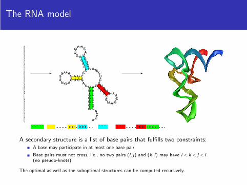
((((((( .. (((( ........ )))) . ((((( ....... ))))) ..... ((((( ....... ))))) ))))))) ....A secondary structure is a list of base pairs that fulfills two constraints:
A base may participate in at most one base pair.
Base pairs must not cross, i.e., no two pairs (i , j) and (k, l) may have i < k < j < l .(no pseudo-knots)
The optimal as well as the suboptimal structures can be computed recursively.
The HP-model
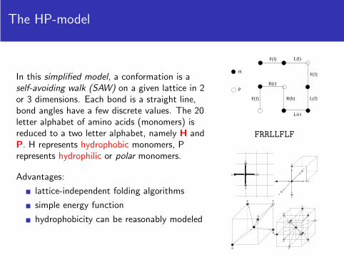
In this simplified model, a conformation is aself-avoiding walk (SAW) on a given lattice in 2or 3 dimensions. Each bond is a straight line,bond angles have a few discrete values. The 20letter alphabet of amino acids (monomers) isreduced to a two letter alphabet, namely H andP. H represents hydrophobic monomers, Prepresents hydrophilic or polar monomers.
Advantages:
lattice-independent folding algorithms
simple energy function
hydrophobicity can be reasonably modeled
H
L(r)
L(f)
F(f)
L(l)F(l)
P
F(f)
R(r)
R(b)
FRRLLFLF
B
L
R
F
U
L
R
B F
D
Q
P F
R
B
Q F
B
L
M
W
Z
Y
P
N
R X
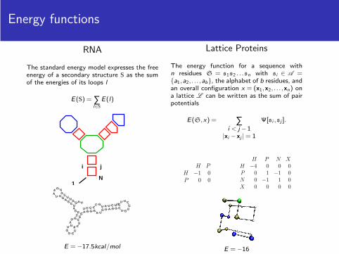
Energy functions
RNA
The standard energy model expresses the freeenergy of a secondary structure S as the sumof the energies of its loops l
E(S) = ∑l∈S
E(l)
1N
i j
UAGG
UU
CG
UGAA
U UG
AG
CUAG CC
GGAUU
GG G
UA C
UCGG
A G G GA U
G U A G G CU G
UG
CUUGUUCUAU
GCCCCU
E = −17.5kcal/mol
Lattice Proteins
The energy function for a sequence withn residues S = s1s2 . . .sn with si ∈ A ={a1,a2, . . . ,ab}, the alphabet of b residues, andan overall configuration x = (x1,x2, . . . ,xn) ona lattice L can be written as the sum of pairpotentials
E(S,x) = ∑i < j −1
|xi −xj | = 1
Ψ[si ,sj ].
H P
H −1 0
P 0 0
H P N X
H −4 0 0 0
P 0 1 −1 0
N 0 −1 1 0
X 0 0 0 0
E = −16
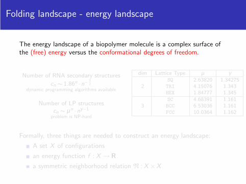
Folding landscape - energy landscape
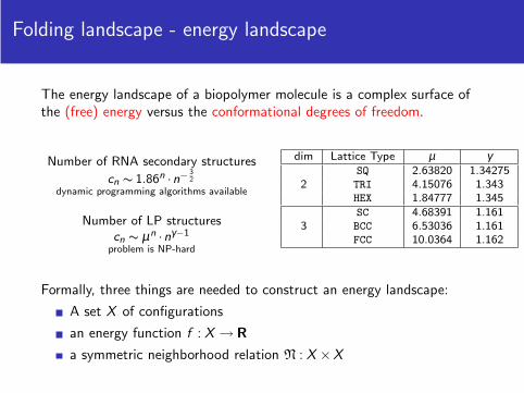
The energy landscape of a biopolymer molecule is a complex surface ofthe (free) energy versus the conformational degrees of freedom.
Number of RNA secondary structures
cn ∼ 1.86n ·n−32
dynamic programming algorithms available
Number of LP structurescn ∼ µn ·nγ−1
problem is NP-hard
dim Lattice Type µ γSQ 2.63820 1.34275
2 TRI 4.15076 1.343HEX 1.84777 1.345SC 4.68391 1.161
3 BCC 6.53036 1.161FCC 10.0364 1.162
Formally, three things are needed to construct an energy landscape:
A set X of configurations
an energy function f : X → R
a symmetric neighborhood relation N : X ×X
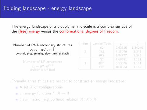
Folding landscape - energy landscape
The energy landscape of a biopolymer molecule is a complex surface ofthe (free) energy versus the conformational degrees of freedom.
Number of RNA secondary structures
cn ∼ 1.86n ·n−32
dynamic programming algorithms available
Number of LP structurescn ∼ µn ·nγ−1
problem is NP-hard
dim Lattice Type µ γSQ 2.63820 1.34275
2 TRI 4.15076 1.343HEX 1.84777 1.345SC 4.68391 1.161
3 BCC 6.53036 1.161FCC 10.0364 1.162
Formally, three things are needed to construct an energy landscape:
A set X of configurations
an energy function f : X → R
a symmetric neighborhood relation N : X ×X
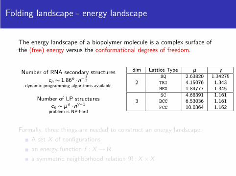
Folding landscape - energy landscape
The energy landscape of a biopolymer molecule is a complex surface ofthe (free) energy versus the conformational degrees of freedom.
Number of RNA secondary structures
cn ∼ 1.86n ·n−32
dynamic programming algorithms available
Number of LP structurescn ∼ µn ·nγ−1
problem is NP-hard
dim Lattice Type µ γSQ 2.63820 1.34275
2 TRI 4.15076 1.343HEX 1.84777 1.345SC 4.68391 1.161
3 BCC 6.53036 1.161FCC 10.0364 1.162
Formally, three things are needed to construct an energy landscape:
A set X of configurations
an energy function f : X → R
a symmetric neighborhood relation N : X ×X

The move set
oo
o
oo
o
o o
oo
o
o o
o o
oo
o
o o
o o
FRLLRLFRR FRLLFLFRR
FUDLUDLU FURLUDLU
For each move there must be an inverse move
Resulting structure must be in X
Move set must be ergodic
Energy barriers and barrier trees
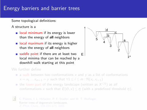
Some topological definitions:
A structure is a
local minimum if its energy is lowerthan the energy of all neighbors
local maximum if its energy is higherthan the energy of all neighbors
saddle point if there are at least twolocal minima thar can be reached by adownhill walk starting at this point
23
45
1*
a
cb
d
E
We further define
a walk between two conformations x and y as a list of conformationsx = x1 . . .xm+1 = y such that ∀1 ≤ i ≤ m : N(xi ,xi+1)
the lower part of the energy landscape (written as X≤η ) as all
conformations x such that E(S,x) ≤ η (with a predefined threshold η).
C. Flamm, I. L. Hofacker, P. F. Stadler, and M. T. Wolfinger.
Barrier trees of degenerate landscapes.Z. Phys. Chem., 216:155–173, 2002.
Energy barriers and barrier trees
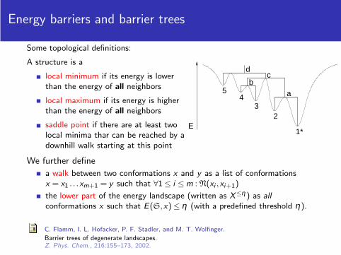
Some topological definitions:
A structure is a
local minimum if its energy is lowerthan the energy of all neighbors
local maximum if its energy is higherthan the energy of all neighbors
saddle point if there are at least twolocal minima thar can be reached by adownhill walk starting at this point
23
45
1*
a
cb
d
E
We further define
a walk between two conformations x and y as a list of conformationsx = x1 . . .xm+1 = y such that ∀1 ≤ i ≤ m : N(xi ,xi+1)
the lower part of the energy landscape (written as X≤η ) as all
conformations x such that E(S,x) ≤ η (with a predefined threshold η).
C. Flamm, I. L. Hofacker, P. F. Stadler, and M. T. Wolfinger.
Barrier trees of degenerate landscapes.Z. Phys. Chem., 216:155–173, 2002.
The lower part of the energy landscape
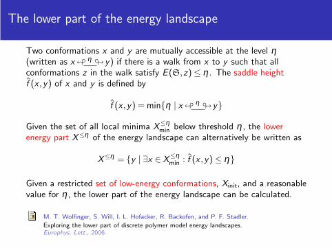
Two conformations x and y are mutually accessible at the level η(written as x "
η#y) if there is a walk from x to y such that all
conformations z in the walk satisfy E (S,z) ≤ η . The saddle heightf̂ (x ,y) of x and y is defined by
f̂ (x ,y) = min{η | x "η
#y}
Given the set of all local minima X≤ηmin below threshold η , the lower
energy part X≤η of the energy landscape can alternatively be written as
X≤η = {y | ∃x ∈ X≤ηmin : f̂ (x ,y) ≤ η}
Given a restricted set of low-energy conformations, Xinit, and a reasonablevalue for η , the lower part of the energy landscape can be calculated.
M. T. Wolfinger, S. Will, I. L. Hofacker, R. Backofen, and P. F. Stadler.
Exploring the lower part of discrete polymer model energy landscapes.Europhys. Lett., 2006.

The Flooder approach
������������������������������������������������������������������������������������������������������������������������������������������������������������������������������������������������������������������������������������������������������������������������������������������������������������������������������������������������������������������������������������������������������������������������������������������������������������������������������������������������������������������������������������������������������������������������������������������������������������������������������������������������������������������������������������������������������������������������������������������������������������������������������������������������������������������������������������������������������������������������������������������������������������������������������������������������������������������������������������������������
������������������������������������������������������������������������������������������������������������������������������������������������������������������������������������������������������������������������������������������������������������������������������������������������������������������������������������������������������������������������������������������������������������������������������������������������������������������������������������������������������������������������������������������������������������������������������������������������������������������������������������������������������������������������������������������������������������������������������������������������������������������������������������������������������������������������������������������������������������������������������������������������������������������������������������������������������������������������������������������������
E
Ep
C
B
D
A������������������������������������������������������������������������������������������������������������������������������������������������������������������������������������������������������������������������������������������������������������������������������������������������������������������������������������������������������������������������������������������������������������������������������������������������������������������������������������������������������������������������������������������������������������������������������������������������������������������������������������������������������������������������������������������������������������������������������������������������������������������������������������������������������������������������������������������������������������������������������������������������������������������������������������������������������������������������������������������������������������������������������������������������
������������������������������������������������������������������������������������������������������������������������������������������������������������������������������������������������������������������������������������������������������������������������������������������������������������������������������������������������������������������������������������������������������������������������������������������������������������������������������������������������������������������������������������������������������������������������������������������������������������������������������������������������������������������������������������������������������������������������������������������������������������������������������������������������������������������������������������������������������������������������������������������������������������������������������������������������������������������������������������������������������������������������������������������������
A
B
C
D
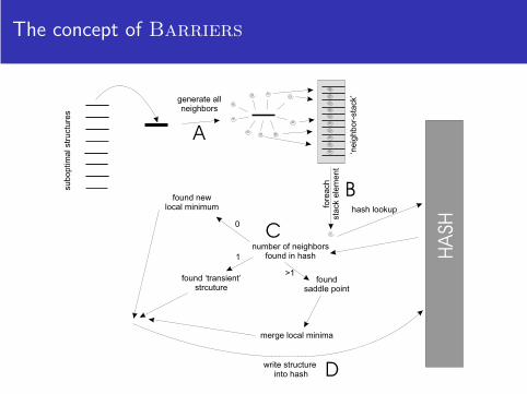
The concept of Barriers
The algorithm of Barriers
Barriers
Require: all suboptimal secondary structures within a certain energy range from mfe1: B ⇐ /02: for all x ∈ subopt do
3: K ⇐ /04: N ⇐ generate neighbors(x)5: for all y ∈ N do
6: if b ⇐ lookup hash(y) then
7: K ⇐ K ∪b
8: end if
9: end for
10: if K = /0 then
11: B ⇐ B∪{x}12: end if
13: if |K | ≥ 2 then
14: merge basins(K )15: end if
16: write hash(x)17: end for
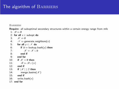
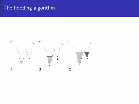
The flooding algorithm
1
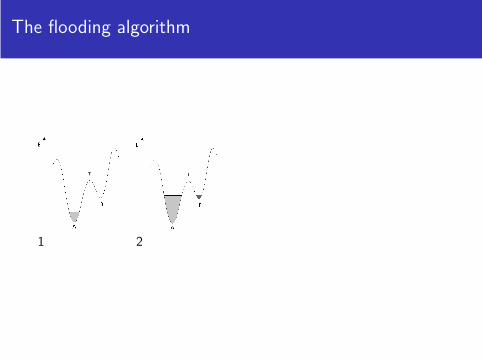
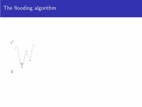
The flooding algorithm
1 2
The flooding algorithm
1 2 3
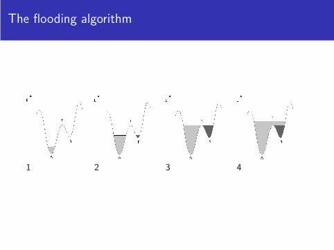
The flooding algorithm
1 2 3 4
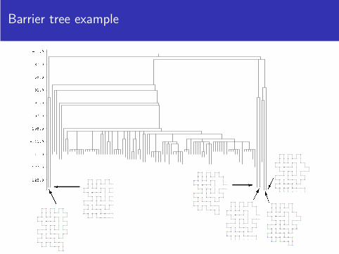
Barrier tree example
Information from the barrier trees
Local minima
Saddle points
Barrier heights
Gradient basins
Partition functions and free energies of (gradient) basins
A gradient basin is the set of all initial points from which a gradient walk(steepest descent) ends in the same local minimum.
Folding kinetics
Biomolecules may have kinetic traps which prevent them from reachingequilibrium within the lifetime of the molecule. Long molecules are oftentrapped in such meta-stable states during transcription.
Possible solutions are
Stochastic folding simulations (predict folding pathways)
Predicting structures for growing fragments of the sequence
Analysis of the energy landscape based on complete suboptimalfolding

Biopolymer dynamics
The probability distribution P of structures as a function of time is ruledby a set of forward equations, also known as the master equation
dPt(x)
dt= ∑
y 6=x
[Pt(y)kxy −Pt(x)kyx ]
Given an initial population distribution, how does the system evolve intime? (What is the population distribution after n time-steps?)
d
dtPt = UPt =⇒ Pt = etUP0
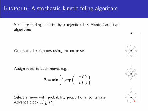
Kinfold: A stochastic kinetic foling algorithm
Simulate folding kinetics by a rejection-less Monte-Carlo typealgorithm:
Generate all neighbors using the move-set
Assign rates to each move, e.g.
Pi = min
{
1,exp
(
−∆E
kT
)}
Select a move with probability proportional to its rateAdvance clock 1/∑i Pi .
P4
P3
P5P6
P7
P8
P1 P2
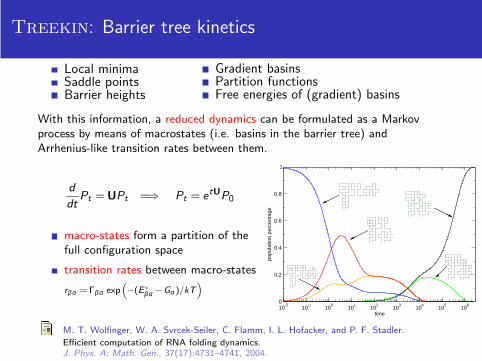
Treekin: Barrier tree kinetics
Local minimaSaddle pointsBarrier heights
Gradient basinsPartition functionsFree energies of (gradient) basins
With this information, a reduced dynamics can be formulated as a Markovprocess by means of macrostates (i.e. basins in the barrier tree) andArrhenius-like transition rates between them.
d
dtPt = UPt =⇒ Pt = etUP0
macro-states form a partition of thefull configuration space
transition rates between macro-states
rβα = Γβα exp(
−(E ∗βα −Gα )/kT
)
10-2
10-1
100
101
102
103
104
105
106
time
0
0.2
0.4
0.6
0.8
1
popu
latio
n pe
rcen
tage
✟✟✟✙
✟✟✟✟✙
❍❍❍❍❥
❍❍❍❍❥
��✠
M. T. Wolfinger, W. A. Svrcek-Seiler, C. Flamm, I. L. Hofacker, and P. F. Stadler.
Efficient computation of RNA folding dynamics.J. Phys. A: Math. Gen., 37(17):4731–4741, 2004.

Dynamics of a short artificial RNA
CUGCGGCUUUGGCUCUAGCC n = 20
1
2
3
45
6 789
10
11
12
1314 15
1617
18 19
20
21
22232425 26
27
28
29
30
3132
33
34
-4.0
-2.0
0.0
2.0
4.0
6.0
10-2
10-1
100
101
102
103
104
time
0
0.2
0.4
0.6
0.8
1
popu
latio
n pr
obab
ility
mfe23458

Dynamics of tRNA
GCGGAUUUAGCUCAGDDGGGAGAGCGCCAGACUGAAYAUCUGGAGGUCCUGUGTPCGAUCCACAGAAUUCGCACCA
100
101
102
103
104
105
106
107
108
time
0
0.2
0.4
0.6
0.8
1
popu
latio
n pr
obab
ility
mfe58056
103
104
105
106
107
108
109
1010
time
0
0.2
0.4
0.6
0.8
1
popu
latio
n pr
obab
ility
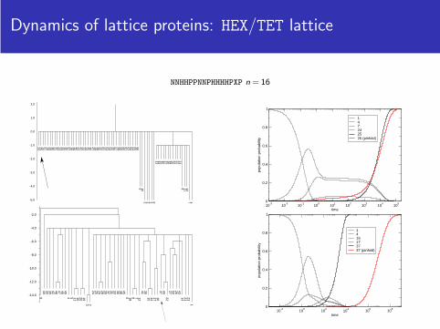
Dynamics of lattice proteins: HEX/TET lattice
NNHHPPNNPHHHHPXP n = 16
12 3 4 5 6 7
89 10 11 12
13 14 15 16 17 18 19 20 21 22 23
24 25 26 27 28 29 30 31 32 33 34 35 36 37 38 39 40 41 42 43 44 45 46 47 48 49 50 51 52 53 54 55 56 57 58 59 60 61 62 63 64 65 66
-5.0
-4.0
-3.0
-2.0
-1.0
0.0
1.0
2.0
NNHHPPNNPHHHHPXP n = 16
123
4 5 6 789 1011 12 131415 1617181920 2122 23
24 25 26272829 30 3132 3334 3536 37383940 4142 434445464748 49 50
-14.0
-12.0
-10.0
-8.0
-6.0
-4.0
-2.0
10-3
10-2
10-1
100
101
102
103
104
105
time
0
0.2
0.4
0.6
0.8
1
popu
latio
n pr
obab
ility
147242525 (pinfold)
10-2
100
102
104
106
108
time
0
0.2
0.4
0.6
0.8
1
popu
latio
n pr
obab
ility
1416173737 (pinfold)
Barrier tree kinetics - problems and pitfalls
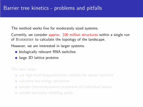
The method works fine for moderately sized systems.
Currently, we consider approx. 100 million structures within a single runof Barriers to calculate the topology of the landscape.
However, we are interested in larger systems:
biologically relevant RNA switches
large 3D lattice proteins
The next steps:
use high-level diagonalization routines for sparse matrices
calculate low-energy structures
sample (thermodynamics properties of) individual basins
sample low-enery refolding paths
Barrier tree kinetics - problems and pitfalls
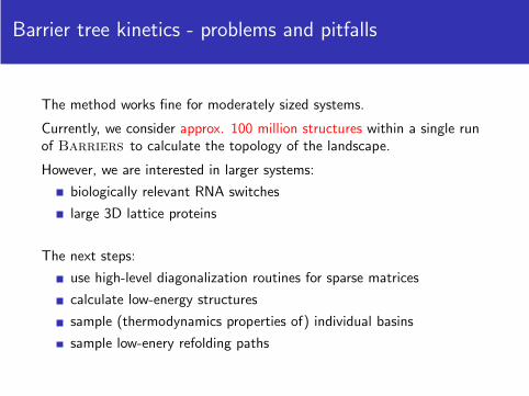
The method works fine for moderately sized systems.
Currently, we consider approx. 100 million structures within a single runof Barriers to calculate the topology of the landscape.
However, we are interested in larger systems:
biologically relevant RNA switches
large 3D lattice proteins
The next steps:
use high-level diagonalization routines for sparse matrices
calculate low-energy structures
sample (thermodynamics properties of) individual basins
sample low-enery refolding paths
The PathFinder tool
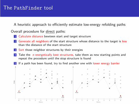
A heuristic approach to efficiently estimate low-energy refolding paths
Overall procedure for direct paths:1 Calculate distance bewteen start and target structure
2 Generate all neighbors of the start structure whose distance to the target is lessthan the distance of the start structure
3 Sort those neighbor structures by their energies
4 Take the n energetically best structures, take them as new starting points andrepeat the procedure until the stop structure is found
5 If a path has been found, try to find another one with lower energy barrier
012345678
Distance
Ene
rgy
START
STOP
012345678
Distance
Ene
rgy
START
STOP
PathFinder example - SV11
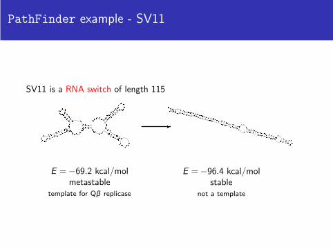
SV11 is a RNA switch of length 115
E = −69.2 kcal/molmetastable
template for Qβ replicase
E = −96.4 kcal/molstable
not a template
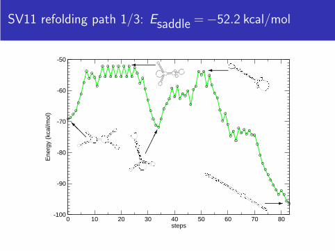
SV11 refolding path 1/3: Esaddle = −52.2 kcal/mol
0 10 20 30 40 50 60 70 80steps
-100
-90
-80
-70
-60
-50
Ene
rgy
(kca
l/mol
)
❅❅❅■
✲
✛
✁✁✁✁✕
✛
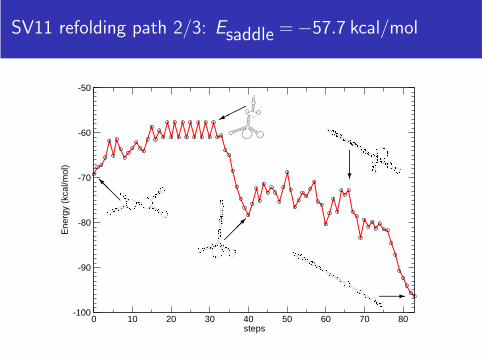
SV11 refolding path 2/3: Esaddle = −57.7 kcal/mol
0 10 20 30 40 50 60 70 80steps
-100
-90
-80
-70
-60
-50
Ene
rgy
(kca
l/mol
)
❅❅❅■
✲
✟✟✟✙
���✒
❄
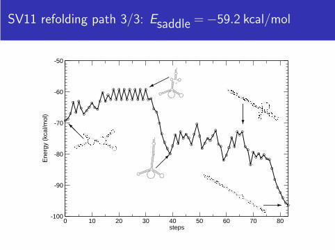
SV11 refolding path 3/3: Esaddle = −59.2 kcal/mol
0 10 20 30 40 50 60 70 80steps
-100
-90
-80
-70
-60
-50
Ene
rgy
(kca
l/mol
)
❅❅❅■
✲
✟✟✟✙
GGG
CACCCCCCUUCGGGGGGUCA
CCUCGCGUAGCUA G
C U A C G C G A G GGU
UAAAG
G G C CUUUC
UC
C C U C G C G UA
G C UAA
CCACGCGAGGUGACCCCCCGAAAAGGGGGGU
UU
CCCA
��✒
❄
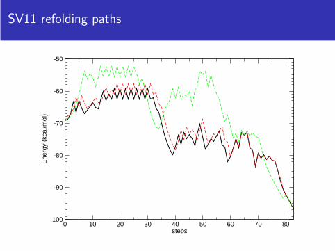
SV11 refolding paths
0 10 20 30 40 50 60 70 80steps
-100
-90
-80
-70
-60
-50
Ene
rgy
(kca
l/mol
)
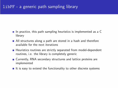
libPF - a generic path sampling library
In practice, this path sampling heuristics is implemented as a Clibrary
All structures along a path are stored in a hash and thereforeavailable for the next iterations
Heuristics routines are strictly separated from model-dependentroutines, i.e. the library is completely generic
Currently, RNA secondary structures and lattice proteins areimplemented
It is easy to extend the functionality to other discrete systems
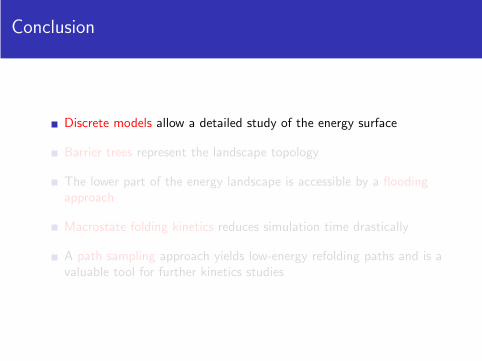
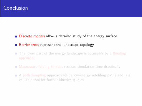
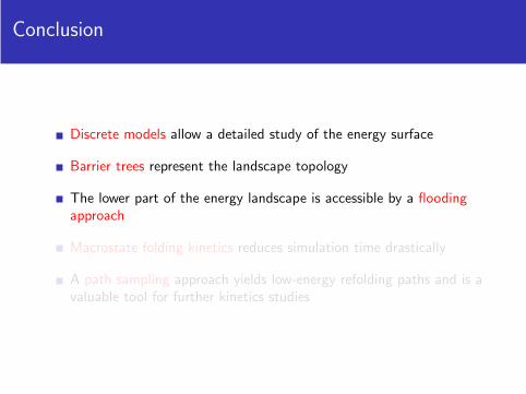
Conclusion
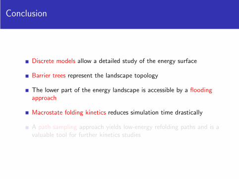
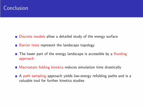
Discrete models allow a detailed study of the energy surface
Barrier trees represent the landscape topology
The lower part of the energy landscape is accessible by a floodingapproach
Macrostate folding kinetics reduces simulation time drastically
A path sampling approach yields low-energy refolding paths and is avaluable tool for further kinetics studies
Conclusion
Discrete models allow a detailed study of the energy surface
Barrier trees represent the landscape topology
The lower part of the energy landscape is accessible by a floodingapproach
Macrostate folding kinetics reduces simulation time drastically
A path sampling approach yields low-energy refolding paths and is avaluable tool for further kinetics studies
References
Christoph Flamm, Ivo Hofacker, Peter StadlerRolf Backofen, Sebastian Will, Martin Mann
M. T. Wolfinger, W. A. Svrcek-Seiler, C. Flamm, I. L. Hofacker, and P. F. Stadler.
Efficient computation of RNA folding dynamics.J. Phys. A: Math. Gen., 37(17):4731–4741, 2004.
M. T. Wolfinger, S. Will, I. L. Hofacker, R. Backofen, and P. F. Stadler.
Exploring the lower part of discrete polymer model energy landscapes.Europhys. Lett., 74(4):725–732, 2006.
Ch. Flamm, W. Fontana, I.L. Hofacker, and P. Schuster.
RNA folding at elementary step resolution.RNA, 6:325–338, 2000
C. Flamm, I. L. Hofacker, P. F. Stadler, and M. T. Wolfinger.
Barrier trees of degenerate landscapes.Z. Phys. Chem., 216:155–173, 2002.