Large variance and fat tail of damage by natural disaster

Large variance and fat tail of damage by natural disaster

Hang-Hyun Jo1,2 and Yu-li Ko3

1Dept. of Physics, Pohang University of Science and Technology, Republic of Korea2Dept. of Computer Science, Aalto University School of Science, Finland

3Dept. of Economics, Rensselaer Polytechnic Institute, USA

The 3rd International Workshop on Physics of Social ComplexityPohang, Korea, May 27, 2016

Extreme events occur!

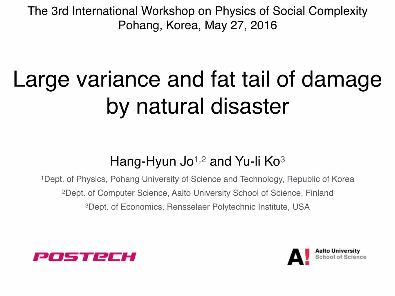
Statistics of damage

Nishenko & Barton, USGS (1995)

Cum

ulat

ive

Num

ber o

f Eve

nts/

Year

p o

TI

D) r-+

D) V) m

o

o o

o

o o

o

o

o

o o 3 o D) o o h C ^ "

Q.

tt> 3" -* c^ C/5 2 Si c g 0} TI

0} -+

0}

Statistics of damage

10-8

10-6

10-4

10-2

100

100 101 102 103

P(D

)

D

(a)

γ=1.93(7)

γ=2.03(4)

deathinjured

10-10

10-8

10-6

10-4

10-2

100

100 101 102 103 104 105 106

P(D

)

D

(b)

γ=1.49(6)

γ=1.55(7)

propertycrop

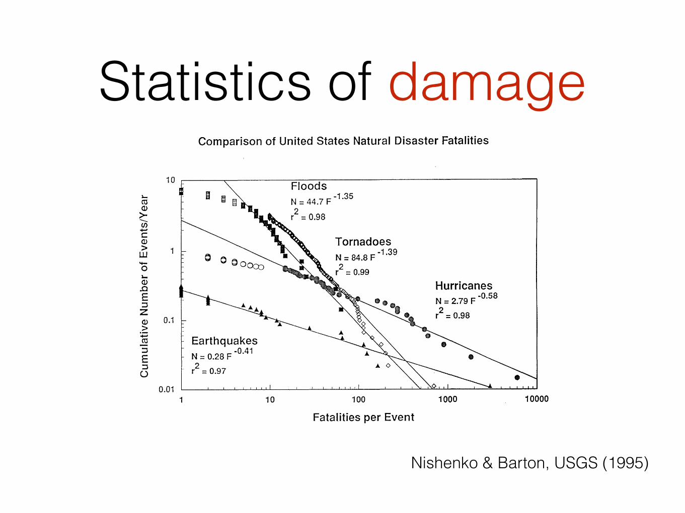
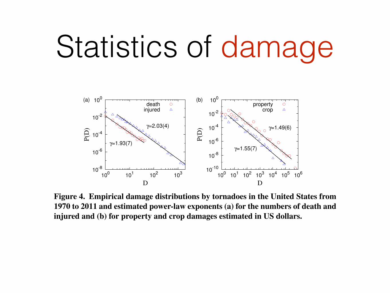
Figure 4. Empirical damage distributions by tornadoes in the United States from1970 to 2011 and estimated power-law exponents (a) for the numbers of death andinjured and (b) for property and crop damages estimated in US dollars.

configurations may enhance the variance of damage by introducing more fluctuationsin exposed values when the tail of value distribution is sufficiently fat (↵ < 2). On theother hand, the randomness may reduce the variance of damage by mixing the valueswhen the tail of value distribution is sufficiently thin (↵ > 2). The former explains theanalytic expectation that the damage will have fatter tails for more correlated configu-rations, while the latter does the numerical observations of the opposite tendency.

Empirical results. In order to support our results, we empirically study casualty andproperty damage distributions by tornadoes in the United States from 1970 to 2011, forwhich the data were retrieved on 24 June 2011 from the website of National ClimaticData Center. By assuming a power-law form for those distributions, the power-lawexponents are estimated as � ⇡ 2 for the numbers of death and the injured, and � ⇡ 1.5

for property and crop damages, as shown in Fig. 4. The significantly different valuesof power-law exponent, i.e., 1.5 and 2, could imply that they represent qualitativelydifferent underlying mechanisms or origins.

In order to account for these observations for tornadoes, our simple model can beextended to take into account various factors like position-dependent vulnerability. Forexample, let us consider that the vulnerability at a site scales with the value at that siteas A ⇠ v

⌘, where the scaling exponent ⌘ can be positive or negative depending on thesituation. Since the effective value, denoted by v

0 ⌘ Av, is proportional to v

1+⌘, the fattail of the PDF of effective value is characterized by the power-law exponent ↵0

=

↵+⌘

1+⌘

.Note that ↵0 reduces to ↵ for ⌘ = 0 as in our simplest setup. More detailed analysis forthe effect of position-dependent vulnerability is left for future works.

CONCLUSION

We have developed a simple model to show that damages by natural disasters couldhave large variances in terms of fat-tailed distributions of natural disaster and popu-lation/property, as well as in terms of their spatial correlations. The damage has been

2752Vulnerability, Uncertainty, and Risk ©ASCE 2014

Vulnerability, Uncertainty, and Risk

Dow

nloa

ded

from

asc

elib

rary

.org

by

Uni

vers

ity o

f Liv

erpo

ol o

n 07

/08/

14. C

opyr

ight

ASC

E. F

or p

erso

nal u

se o

nly;

all

right

s res

erve

d.

Extreme events occur!

damage = natural disaster × population/property × vulnerability

Stromberg, J. Econ. Perspect. (2007)

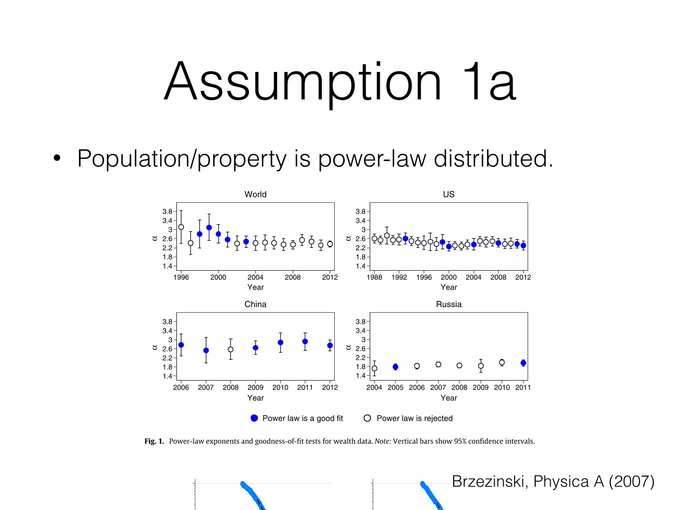
Assumption 1a• Population/property is power-law distributed.

158 M. Brzezinski / Physica A 406 (2014) 155–162

αα

αα

Fig. 1. Power-law exponents and goodness-of-fit tests for wealth data. Note: Vertical bars show 95% confidence intervals.

Fig. 2. The complementary cumulative distribution functions and their power-law fits.

this purpose. However, as stated by Ref. [32], there is no consensusmethodology to overcome this problem. Our conclusionsapply, therefore, only to the original data taken from the ‘rich lists’, which is, however, the most popular form of data usedin the relevant literature. It is worth noticing here also that the described data correlation does not occur in our data sets forRussia, as no Russian billionaire gained his or her wealth due to inheritance. Still, the power-law hypothesis is inconsistentwith these data sets in all but one case.

Our results are inconsistent with those of Ref. [28], who found that the power-law behaviour of the wealth of the world’srichest persons according to Forbes’ data in every year between 2000 and 2009 is ruled out by conventional goodness-of-fittests. On the contrary, we find that the wealth of the world’s billionaires is fitted well by a power-law model in 2000, 2001,and 2003. This inconsistency can be explained by noticing that Ref. [28] has not estimated the lower bound on the power-law behaviour, xmin, but has fitted power-lawmodels to the whole range of Forbes’ observations. However, fixing xmin at theminimum wealth level in Forbes’ data seems to be statistically unjustified.

Brzezinski, Physica A (2007)

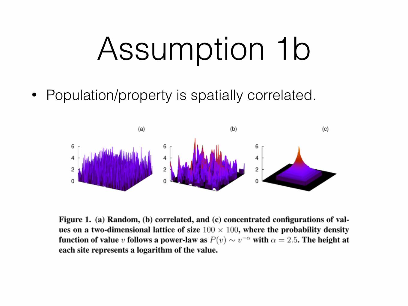
Assumption 1b• Population/property is spatially correlated.

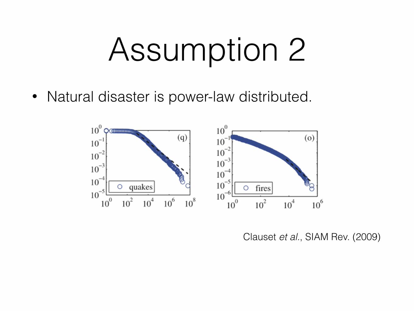
Assumption 2• Natural disaster is power-law distributed.

Clauset et al., SIAM Rev. (2009)

Assumption 3• Vulnerability is constant.

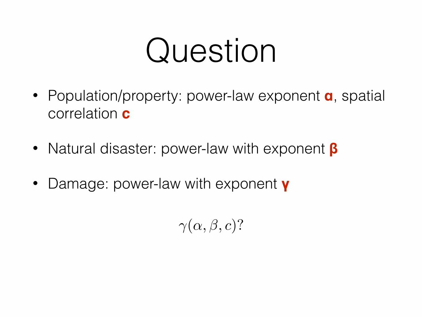
Question• Population/property: power-law exponent α, spatial

correlation c

• Natural disaster: power-law with exponent β

• Damage: power-law with exponent γ

�(↵,�, c)?

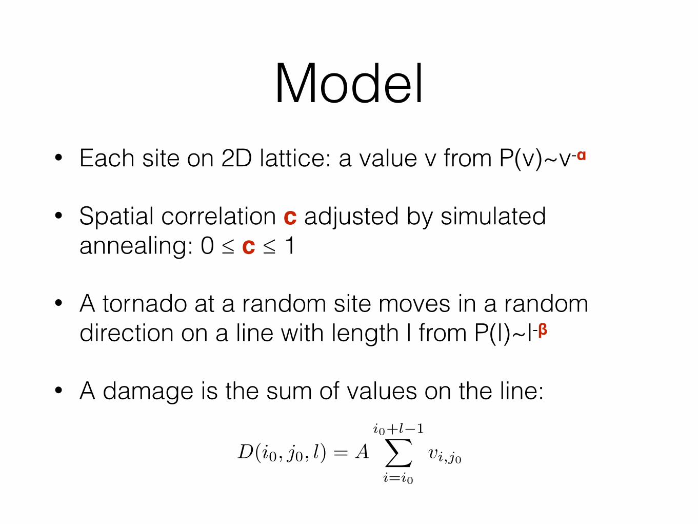
Model• Each site on 2D lattice: a value v from P(v)~v-α

• Spatial correlation c adjusted by simulated annealing: 0 ≤ c ≤ 1

• A tornado at a random site moves in a random direction on a line with length l from P(l)~l-β

• A damage is the sum of values on the line:

D(i0, j0, l) = Ai0+l�1X

i=i0

vi,j0

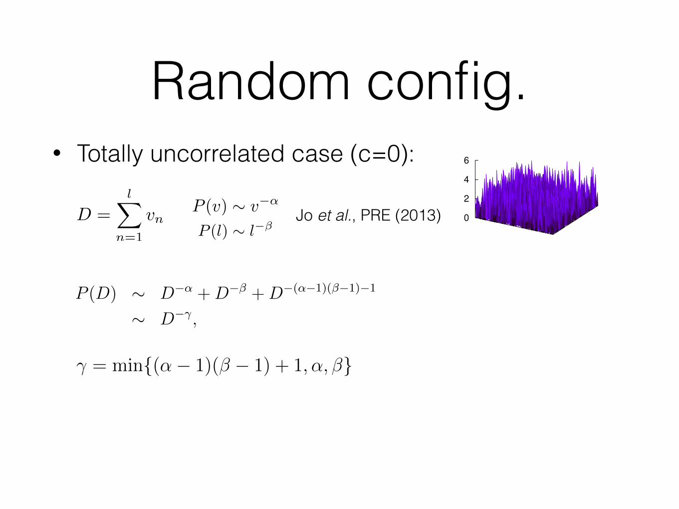
Random config.• Totally uncorrelated case (c=0):

D =lX

n=1

vn

The zero centrality, c = 0, corresponds to the random configuration, while the max-imum centrality, c = 1, implies that the values are concentrated in the central area,i.e., around the origin (0, 0). The configuration with intermediate c is formulated usinga simulated annealing algorithm. Starting from a random configuration, two randomlyselected sites swap their values only if the swapping increases the correlation. Theswapping is repeated until the correlation reaches the desired value of c. Figure 1 showsexemplary configurations of value for random (c = 0), correlated (c ⇡ 0.85), andconcentrated (c = 1) cases.

For natural disasters, we focus on moving disasters like tornadoes that move alonga trajectory. We assume that a disaster initiated at a random site moves in a randomdirection, i.e., one of ±x and ±y directions, over the trajectory with length l. Thelength l is randomly drawn from a distribution P (l) ⇠ l

�� with exponent � > 1.The vulnerability A

i,j

at site (i, j) is assumed to be constant for all sites in the systemsuch that A

i,j

= 1 for all (i, j) for convenience. Then, the damage D by the disasterinitiated at (i

0

, j

0

) and moving l sites, say in the direction of +x-axis, is given as thesum of values over the trajectory:

D(i

0

, j

0

, l) =

i0+l�1X

i=i0

A

i,j0vi,j0 =

i0+l�1X

i=i0

v

i,j0 .

RESULT

It is expected that the damage D has a large variance by showing a fat-tailed distribu-tion, P (D) ⇠ D

�� with exponent �. In general, the value of � depends on exponents↵, �, and the centrality c.

Random configurations. The case of random configurations with zero centrality canbe analytically solved due to its uncorrelated nature (Jo et al., 2013). The damage D isindependent of the initiation position and moving direction of the disaster, hence it canbe written as a sum of l independent and identical random variables, vs:

D =

lX

n=1

v

n

.

For small l, as l is mostly 1, i.e., D = v

1

, we obtain D

�↵ for P (D). For sufficientlylarge l, if the variance of {v

n

} is small, one can approximate as D ⇡ lhvi, where h·idenotes an average, leading to D

�� for P (D). Finally, for sufficiently large l, if thevariance of {v

n

} is large, D is dominated by max{vn

} that is proportional to l

1/(↵�1).By means of the identity P (D)dD = P (l)dl, one gets D

�(↵�1)(��1)�1 for P (D). Weobtain apart from the coefficients

P (D) ⇠ D

�↵

+D

��

+D

�(↵�1)(��1)�1

⇠ D

��

,



Dow

nloa

ded

from

asc

elib

rary

.org

by

Uni

vers

ity o

f Liv

erpo

ol o

n 07

/08/

14. C

opyr

ight

ASC

E. F

or p

erso

nal u

se o

nly;

all

right

s res

erve

d.

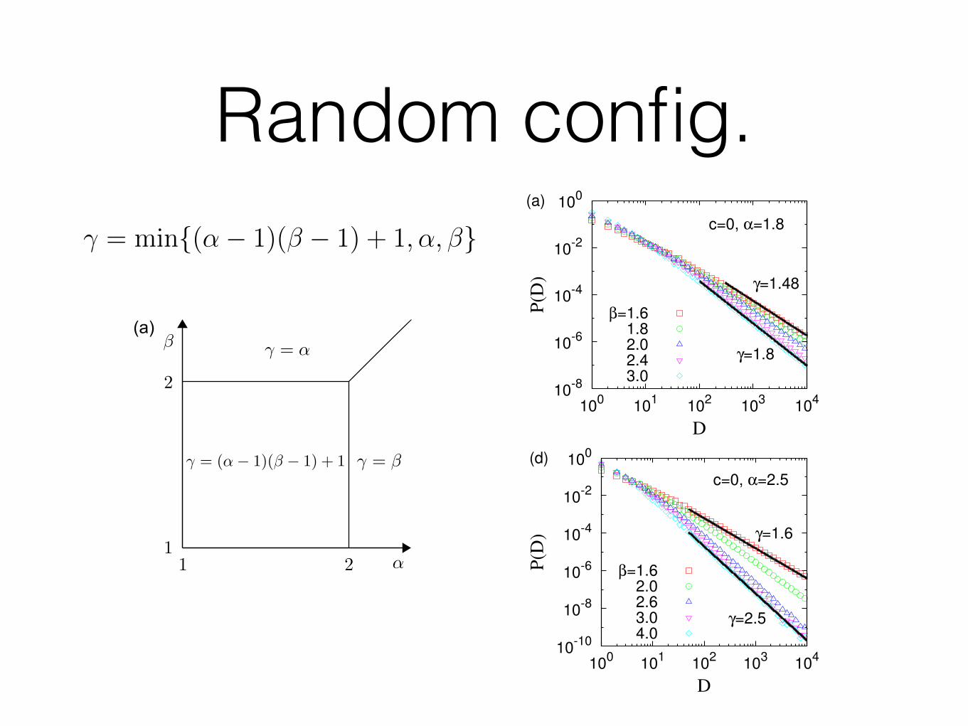
Figure 2. Phase diagrams summarizing analytic results (a) for random configura-tions and (b) for concentrated configurations.

thus for large D,� = min{(↵� 1)(� � 1) + 1,↵, �}, (1)

which is depicted in Fig. 2(a). This solution has been also obtained by rigorous calcu-lations (Jo et al., 2013). In case with ↵ > 2 and ↵ > �, i.e., when the tail of valuedistribution is sufficiently thin, one obtains � = �, implying that statistical propertiesof damage are determined only by those of disaster. In case with � > 2 and � > ↵,one gets � = ↵, implying the dominance of statistical properties of value in decidingdamage. Only when both value and disaster distributions have sufficiently fat tails, i.e.,when ↵, � < 2, the fat tail of damage can be explained in terms of the interplay of bothvalue and disaster. We perform numerical simulations on the square lattice of linear sizeL = 3 · 103 to confirm our analysis as shown in Fig. 3.

Concentrated configurations. Since a concentrated configuration with c = 1 has arotational symmetry around the origin (0, 0), it can be described simply by a function ofthe distance r from the origin, i.e., v(r) ' v

0

r

�µ with µ =

2

↵�1

. The relation µ =

2

↵�1

has been obtained by the identity P (v)dv / 2⇡rdr. For convenience, we calculate D

in a continuum limit of lattice as

D(r

0

, ✓

0

, l,�) ' wv

0

Zl

0

r(t)

�µ

dt,

r(t) =

p(r

0

cos ✓

0

+ t cos�)

2

+ (r

0

sin ✓

0

+ t sin�)

2

,

where the polar coordinate (r

0

, ✓

0

) and the angle � are the initiation position andmoving direction of the disaster, and w denotes the transverse dimension or widthof the disaster. Since r(t) can be written in terms of r

x

⌘ r

0

cos(� � ✓

0

) andr

y

⌘ r

0

sin(�� ✓

0

), we get

D ' wv

0

Zl

0

[(t+ r

x

)

2

+ r

2

y

]

�µ/2

dt. (2)



Dow

nloa

ded

from

asc

elib

rary

.org

by

Uni

vers

ity o

f Liv

erpo

ol o

n 07

/08/

14. C

opyr

ight

ASC

E. F

or p

erso

nal u

se o

nly;

all

right

s res

erve

d.

a location with more disasters if natural phenomena related to a certain disaster canbenefit people despite possible damage by such disaster. For example, coastal area ismore likely to be affected by tsunamis, while it provides ports for trade and fishing.

Thirdly, we consider the vulnerability as a fraction of the realized damage out ofeach unit of population/property. It differs by variables such as wealth, building code,and network structure of infrastructure. Since there are more hospitals and more laborwho are devoted to control disasters in cities, cities could have less vulnerability. Onthe other hand, cities could be more vulnerable due to a cascading effect of damage.In our model, since the property of vulnerability is hard to measure, we assume thatthe vulnerability is constant through the trajectory of disaster. Our model with theassumption of constant vulnerability can provide benchmark results for further realisticrefinements.

Finally, the total damage by a natural disaster is modeled to be as the sum ofpopulation/property exposed to that disaster, multiplied by the vulnerability of thosepopulation/property.

Model setting. We first generate landscapes or configurations of population/propertyon a two-dimensional square lattice of size L⇥ L with a periodic boundary condition,see Fig. 1. The population/property, or a value for convenience, at site (i, j) is denotedby v

i,j

for i, j = �L

2

, · · · , L2

� 1. The PDF of value is assumed to follow a power law,P (v) ⇠ v

�↵ with exponent ↵ > 1. To parameterize the degree of spatial correlation ofvalue, we define a normalized centrality c as a function of value configuration {v}:

c({v}) = E

rand

� E({v})E

rand

� E

conc

, E({v}) =X

i,j

✓��lnv

i,j

v

i+1,j

��+��ln

v

i,j

v

i,j+1

��

◆,

where E measures the total difference between values of neighboring sites. Erand

andE

conc

denote the values of E for random and concentrated configurations, respectively.

0

2

4

6

(a)

0

2

4

6

(b)

0

2

4

6

(c)

Figure 1. (a) Random, (b) correlated, and (c) concentrated configurations of val-ues on a two-dimensional lattice of size 100 ⇥ 100, where the probability densityfunction of value v follows a power-law as P (v) ⇠ v

�↵ with ↵ = 2.5. The height ateach site represents a logarithm of the value.



Dow

nloa

ded

from

asc

elib

rary

.org

by

Uni

vers

ity o

f Liv

erpo

ol o

n 07

/08/

14. C

opyr

ight

ASC

E. F

or p

erso

nal u

se o

nly;

all

right

s res

erve

d.

Jo et al., PRE (2013)P (v) ⇠ v�↵

P (l) ⇠ l��

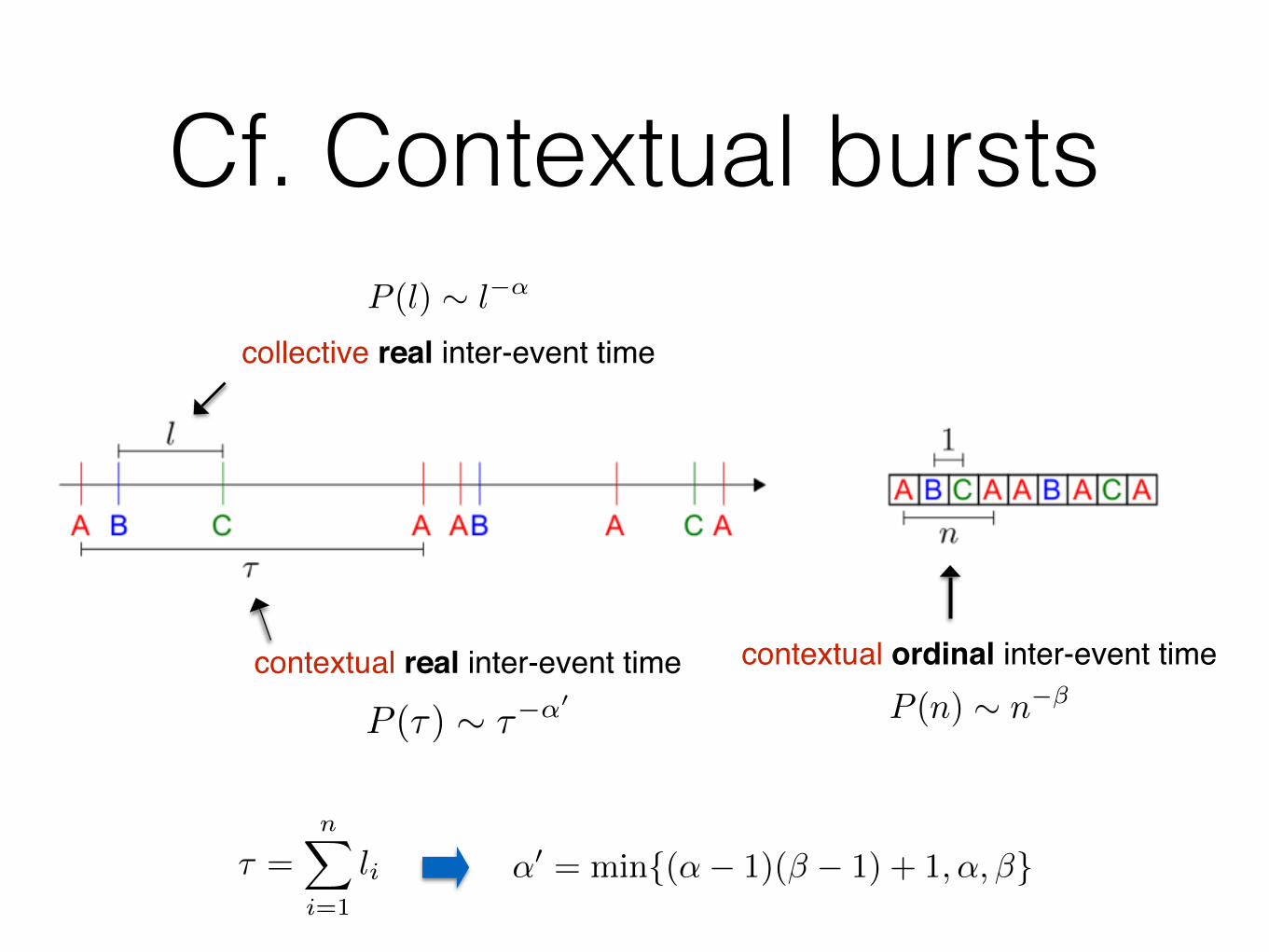
collective real inter-event timeP (l) ⇠ l�↵

contextual real inter-event time

P (⌧) ⇠ ⌧�↵0

contextual ordinal inter-event timeP (n) ⇠ n��

⌧ =nX

i=1

li ↵0 = min{(↵� 1)(� � 1) + 1,↵,�}

Cf. Contextual bursts

Topical Review R199

Particle:

Site:

u(1)u(2)

u(3)

u(1)u(3) u(2)

1 2 3 4

1 2 3 4

5

5

(a)

(b)

Figure 1. Mapping between the zero-range process and the asymmetric exclusion process.

the ZRP with a corresponding configuration of particles in an exclusion model. (The mappingis unique up to translations of the exclusion process lattice.) To do this, one thinks of particlesin the ZRP as vacancies in the exclusion process, and sites in the ZRP as occupied sites in theexclusion process. Thus, in figure 1, site 1 in the ZRP becomes particle 1 in the exclusionprocess. The next three vacancies in the exclusion process represent the particles at site 2in the ZRP and then site 2 itself is represented by particle 2 in the exclusion process, and soon. In this way, one obtains an exclusion model on a lattice containing L + N sites and Lparticles.

The exclusion process dynamics are inferred from the way in which configurations evolvewhen the corresponding ZRP configurations evolve under the ZRP dynamics: the hop ratesin the ZRP, which depend on the number of particles at the departure site, become hop ratesin the exclusion process which depend on the distance to the next particle in front. Thus,depending on the form chosen for u(n), there may be a long-range interaction between theparticles in the exclusion process.

We remark that this mapping relies on the preservation of the order of particles under theexclusion process dynamics, therefore it is only really useful in one dimension.

2.2. Solution of the steady state

One of the most important properties of the ZRP is that its steady state is given by a simplefactorized form. This means that the steady state probability P({nl}) of finding the systemin a configuration {nl} = n1, n2, . . . , nL is given by a product of (scalar) factors f (nl) (onefactor for each site of the system) i.e.,

P({nl}) = Z−1L,N

L!

l=1

f (nl), (2)

where ZL,N is a normalization which ensures that the sum of probabilities for all configurationscontaining N particles is equal to 1, hence

ZL,N ="

{nl}

L!

l=1

f (nl)δ

#L"

l=1

nl − N

$

. (3)

Here, the δ-function has been introduced to guarantee that we only include those configurationscontaining N particles in the sum. Finally, the factors f (nl) are determined by the hop rates:

f (n) =n!

i=1

u(i)−1 for n > 0, f (0) = 1. (4)

We now turn to the proof of the steady state (2) to (4). The first step is to write thesteady state condition that is satisfied by the probabilities P({nl}). This condition balances

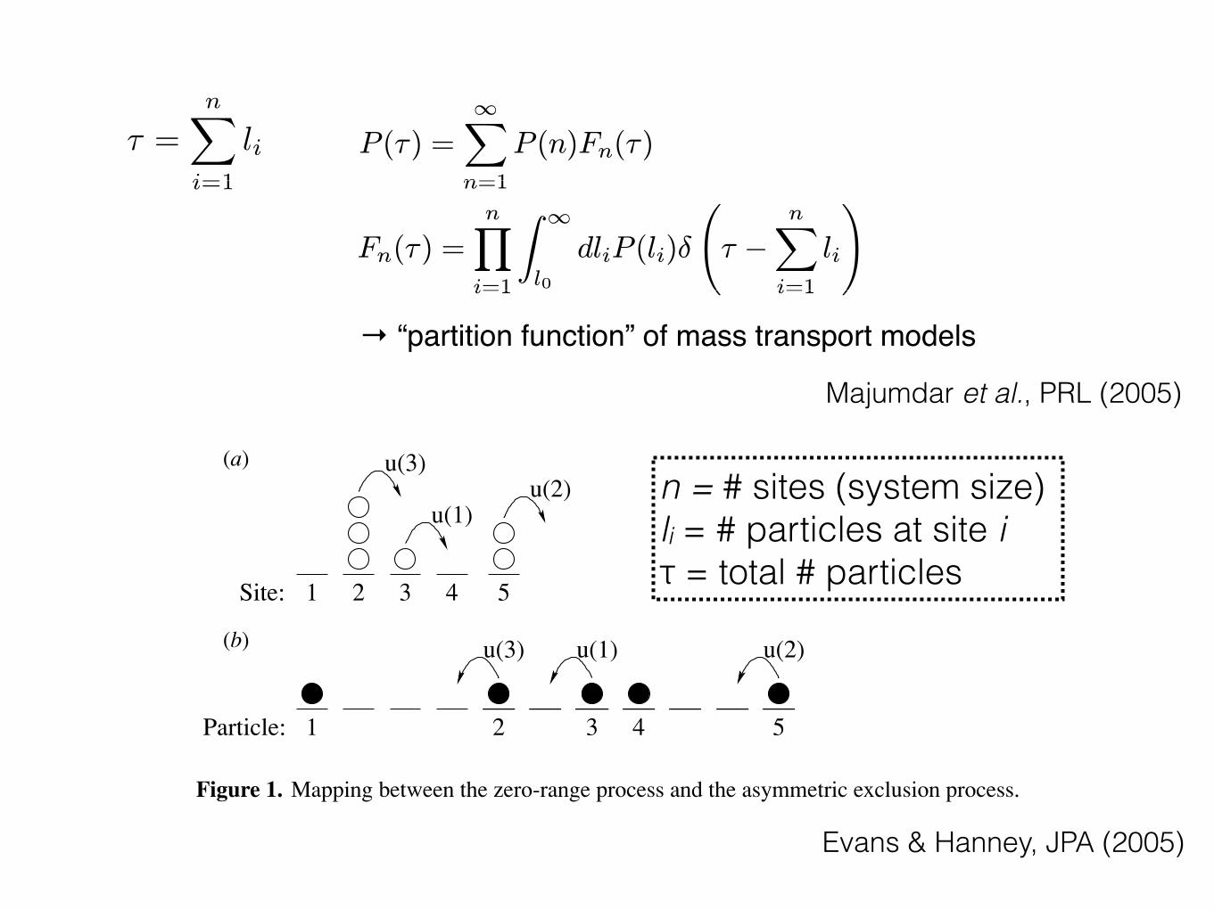
⌧ =nX

i=1

li¿ =

nX

i=1

li P (¿) =

1X

n=1

P (n)Fn(¿)

Fn(¿) =nY

i=1

Z 1

l0

dliP (li)±

Ã¿ ¡

nX

i=1

li

!

→ “partition function” in mass transport models [Majumdar et al., PRL ’05]

[Evans & Hanney, JPA ’05]

¿li

n

Majumdar et al., PRL (2005)

Evans & Hanney, JPA (2005)

→ “partition function” of mass transport models

n = # sites (system size) li = # particles at site i τ = total # particles

Random config.

(a)





0

r

�µ with µ =

2

↵�1

. The relation µ =

2

↵�1



D(r

0

, ✓

0

, l,�) ' wv

0

Zl

0

r(t)

�µ

dt,

r(t) =

p(r

0

cos ✓

0

+ t cos�)

2

+ (r

0

sin ✓

0

+ t sin�)

2

,


0

, ✓

0


x

⌘ r

0

cos(� � ✓

0

) andr

y

⌘ r

0

sin(�� ✓

0

), we get

D ' wv

0

Zl

0

[(t+ r

x

)

2

+ r

2

y

]

�µ/2

dt. (2)



Dow

nloa

ded

from

asc

elib

rary

.org

by

Uni

vers

ity o

f Liv

erpo

ol o

n 07

/08/

14. C

opyr

ight

ASC

E. F

or p

erso

nal u

se o

nly;

all

right

s res

erve

d.

1

1.2

1.4

1.6

1.8

2

1 2 3 4 5

γ

β

(c)α=1.8

analysis: c=0c=1

numeric: c=0t=104

t=5x104

c=1

1

1.5

2

2.5

3

1 2 3 4 5

γ

β

(f)α=2.5

analysisnumeric: c=0

t=104

t=5x104

c=1

10-8

10-6

10-4

10-2

100

100 101 102 103 104

P(D

)

D

(a)

c=0, α=1.8

γ=1.48

γ=1.8

β=1.61.82.02.43.0

10-8

10-6

10-4

10-2

100

100 101 102 103 104

P(D

)

D

(b)

c=1, α=1.8

γ=1.6

γ=1.8

β=1.61.82.02.43.0

10-10

10-8

10-6

10-4

10-2

100

100 101 102 103 104

P(D

)

D

(d)

c=0, α=2.5

γ=1.6

γ=2.5

β=1.62.02.63.04.0

10-10

10-8

10-6

10-4

10-2

100

100 101 102 103 104

P(D

)

D

(e)

c=1, α=2.5

γ=1.6

γ=2.5

β=1.62.02.63.04.0

Figure 3. Numerical results of damage distributions and their power-law expo-nents for ↵ = 1.8 (top) and for ↵ = 2.5 (bottom). In (c) and (f), t denotes the MonteCarlo time in the simulated annealing to generate correlated configurations.

hence it is independent of the spatial correlation or centrality c. The second term D

��

is due to D =

Pl

n=1

v

n

/ l. That is, most disasters move along trajectories consistingof small v

n

s when the tail of P (v) is sufficiently thin, i.e., when ↵ > 2. This leadsto the irrelevance of the spatial correlation. Thus, one can expect that � = min{↵, �}holds for the entire range of c. This is confirmed by numerical simulations for the caseof ↵ = 2.5 in Fig. 3(f), with some deviations mainly due to logarithmic corrections toscaling, like lnD, and finite size effects. It is observed that the estimated values of � aresystematically smaller for larger centrality, implying fatter tails of damage distributions.

For ↵ < 2 and � < 2, the difference in values of � for c = 0 and for c = 1 issummarized as follows:

�� ⌘ �

c=1

� �

c=0

=

⇢(2� ↵)(� � 1) if � < ↵,(↵� 1)(2� �) if � > ↵.

This implies that the tail of damage distribution for the concentrated case is alwaysthinner than that for the random case. The maximum value of the difference �� is 1/4when ↵ = � = 3/2. The numerical simulations for the case of ↵ = 1.8 in Fig. 3(c)confirm the analytic solution, with deviations due to corrections to scaling and finitesize effects. While such deviations seem to be large, we systematically observe that inthe region of � < 2, the values of � for c = 1 are slightly larger than those for c = 0,comparable to the analytic results.

It turns out that whether the spatial correlation of value enhances or reduces thefat tail property of damage is not a simple issue as expected. The randomness in value



Dow

nloa

ded

from

asc

elib

rary

.org

by

Uni

vers

ity o

f Liv

erpo

ol o

n 07

/08/

14. C

opyr

ight

ASC

E. F

or p

erso

nal u

se o

nly;

all

right

s res

erve

d.





0

r

�µ with µ =

2

↵�1

. The relation µ =

2

↵�1



D(r

0

, ✓

0

, l,�) ' wv

0

Zl

0

r(t)

�µ

dt,

r(t) =

p(r

0

cos ✓

0

+ t cos�)

2

+ (r

0

sin ✓

0

+ t sin�)

2

,


0

, ✓

0


x

⌘ r

0

cos(� � ✓

0

) andr

y

⌘ r

0

sin(�� ✓

0

), we get

D ' wv

0

Zl

0

[(t+ r

x

)

2

+ r

2

y

]

�µ/2

dt. (2)



Dow

nloa

ded

from

asc

elib

rary

.org

by

Uni

vers

ity o

f Liv

erpo

ol o

n 07

/08/

14. C

opyr

ight

ASC

E. F

or p

erso

nal u

se o

nly;

all

right

s res

erve

d.

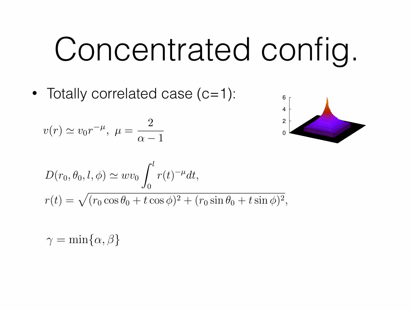
Concentrated config.• Totally correlated case (c=1):





0

r

�µ with µ =

2

↵�1

. The relation µ =

2

↵�1



D(r

0

, ✓

0

, l,�) ' wv

0

Zl

0

r(t)

�µ

dt,

r(t) =

p(r

0

cos ✓

0

+ t cos�)

2

+ (r

0

sin ✓

0

+ t sin�)

2

,


0

, ✓

0


x

⌘ r

0

cos(� � ✓

0

) andr

y

⌘ r

0

sin(�� ✓

0

), we get

D ' wv

0

Zl

0

[(t+ r

x

)

2

+ r

2

y

]

�µ/2

dt. (2)



Dow

nloa

ded

from

asc

elib

rary

.org

by

Uni

vers

ity o

f Liv

erpo

ol o

n 07

/08/

14. C

opyr

ight

ASC

E. F

or p

erso

nal u

se o

nly;

all

right

s res

erve

d.

For small l, the integration is approximated up to the first order of l, leading to D /v

0

r

�µ

0

l ' v(r

0

)l. Thus, we obtain D

�↵

+ D

�� for P (D) apart from the coefficients.For large l, by substituting the variable of integration as t+ r

x

= r

y

tan ✓, one gets

D ' wv

0

r

1�µ

y

Ztan

�1 l+r

x

r

y

tan

�1 r

x

r

y

cos

µ�2

✓d✓.

Note that tan�1

r

x

r

y

=

⇡

2

� (�� ✓

0

). The following formula can be used:

Zcos

µ�2

✓d✓ =

sgn(sin ✓) cosµ�1

✓

2

F

1

(

1

2

,

µ�1

2

;

µ+1

2

; cos

2

✓)

1� µ

+ const.,

where sgn(x) gives the sign of x and2

F

1

is the hypergeometric function. We considertwo cases according to the moving direction of the disaster. In case with |��✓

0

| < ⇡/2,i.e., r

x

> 0, the disaster moves away from the central area. We get the result up to theleading terms as

D ⇡ wv

0

l

1�µ � a

1

r

1�µ

0

1� µ

(3)

with a constant a1

⌘2

F

1

(

1

2

,

µ�1

2

;

µ+1

2

; sin

2

(� � ✓

0

)). If µ > 1 (↵ < 3), from D ⇠r

1�µ

0

⇠ v

µ�1µ , we have the term D

�↵+13�↵ for P (D). This is dominated by D

�↵ because↵+1

3�↵

> ↵ for ↵ < 3. If µ < 1 (↵ > 3), D ⇠ l

1�µ leads to the term D

� (↵�1)(��1)↵�3 �1 for

P (D), which is dominated by D

�� for � > 1. On the other hand, for |� � ✓

0

| > ⇡/2,i.e., r

x

< 0, the disaster approaches the central area to some extent and eventuallymoves away. The domain of integration in Eq. (2) can be divided into two at the closestposition of the disaster to the origin given by t⇥ ⌘ �r

x

:Z

l

t⇥

dt Z

l

0

dt =

Zt⇥

0

dt+

Zl

t⇥

dt 2

Zl

t⇥

dt.

Here the second inequality holds for sufficiently large l. Similarly to the case with|� � ✓

0

| < ⇡/2, we get the same result up to the leading terms as Eq. (3) but with a

1

replaced by a

2

⌘ sin

1�µ

(��✓

0

)�(

µ+1

2

)�(

1

2

)/�(

µ

2

). Finally, since P (D) ⇠ D

�↵

+D

�� ,we obtain the result for � as

� = min{↵, �}. (4)

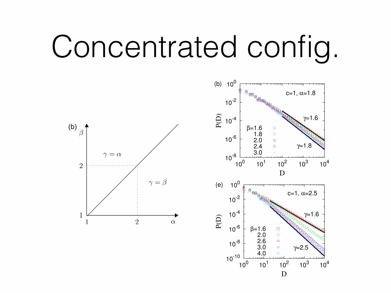
This solution is depicted in Fig. 2(b), and confirmed by numerical simulations as shownin Fig. 3.

Correlated configurations. Before investigating the effect of correlated configura-tions with 0 < c < 1, we compare the results for random and concentrated cases,Eqs. (1, 4). If ↵ > 2 or � > 2, we get � = min{↵, �} from P (D) ⇠ D

�↵

+D

�� forboth cases of c = 0 and c = 1. The first term D

�↵ is mainly due to D = v when l = 1,



Dow

nloa

ded

from

asc

elib

rary

.org

by

Uni

vers

ity o

f Liv

erpo

ol o

n 07

/08/

14. C

opyr

ight

ASC

E. F

or p

erso

nal u

se o

nly;

all

right

s res

erve

d.

a location with more disasters if natural phenomena related to a certain disaster canbenefit people despite possible damage by such disaster. For example, coastal area ismore likely to be affected by tsunamis, while it provides ports for trade and fishing.

Thirdly, we consider the vulnerability as a fraction of the realized damage out ofeach unit of population/property. It differs by variables such as wealth, building code,and network structure of infrastructure. Since there are more hospitals and more laborwho are devoted to control disasters in cities, cities could have less vulnerability. Onthe other hand, cities could be more vulnerable due to a cascading effect of damage.In our model, since the property of vulnerability is hard to measure, we assume thatthe vulnerability is constant through the trajectory of disaster. Our model with theassumption of constant vulnerability can provide benchmark results for further realisticrefinements.

Finally, the total damage by a natural disaster is modeled to be as the sum ofpopulation/property exposed to that disaster, multiplied by the vulnerability of thosepopulation/property.

Model setting. We first generate landscapes or configurations of population/propertyon a two-dimensional square lattice of size L⇥ L with a periodic boundary condition,see Fig. 1. The population/property, or a value for convenience, at site (i, j) is denotedby v

i,j

for i, j = �L

2

, · · · , L2

� 1. The PDF of value is assumed to follow a power law,P (v) ⇠ v

�↵ with exponent ↵ > 1. To parameterize the degree of spatial correlation ofvalue, we define a normalized centrality c as a function of value configuration {v}:

c({v}) = E

rand

� E({v})E

rand

� E

conc

, E({v}) =X

i,j

✓��lnv

i,j

v

i+1,j

��+��ln

v

i,j

v

i,j+1

��

◆,

where E measures the total difference between values of neighboring sites. Erand

andE

conc

denote the values of E for random and concentrated configurations, respectively.

0

2

4

6

(a)

0

2

4

6

(b)

0

2

4

6

(c)

Figure 1. (a) Random, (b) correlated, and (c) concentrated configurations of val-ues on a two-dimensional lattice of size 100 ⇥ 100, where the probability densityfunction of value v follows a power-law as P (v) ⇠ v

�↵ with ↵ = 2.5. The height ateach site represents a logarithm of the value.



Dow

nloa

ded

from

asc

elib

rary

.org

by

Uni

vers

ity o

f Liv

erpo

ol o

n 07

/08/

14. C

opyr

ight

ASC

E. F

or p

erso

nal u

se o

nly;

all

right

s res

erve

d.

v(r) ' v0r�µ, µ =

2

↵� 1

Concentrated config.

1

1.2

1.4

1.6

1.8

2

1 2 3 4 5

γ

β

(c)α=1.8

analysis: c=0c=1

numeric: c=0t=104

t=5x104

c=1

1

1.5

2

2.5

3

1 2 3 4 5

γ

β

(f)α=2.5


t=104

t=5x104

c=1

10-8

10-6

10-4

10-2

100

100 101 102 103 104

P(D

)

D

(a)

c=0, α=1.8

γ=1.48

γ=1.8

β=1.61.82.02.43.0

10-8

10-6

10-4

10-2

100

100 101 102 103 104

P(D

)

D

(b)

c=1, α=1.8

γ=1.6

γ=1.8

β=1.61.82.02.43.0

10-10

10-8

10-6

10-4

10-2

100

100 101 102 103 104

P(D

)

D

(d)

c=0, α=2.5

γ=1.6

γ=2.5

β=1.62.02.63.04.0

10-10

10-8

10-6

10-4

10-2

100

100 101 102 103 104

P(D

)

D

(e)

c=1, α=2.5

γ=1.6

γ=2.5

β=1.62.02.63.04.0



��

is due to D =

Pl

n=1

v

n


n



�� ⌘ �

c=1

� �

c=0

=

⇢(2� ↵)(� � 1) if � < ↵,(↵� 1)(2� �) if � > ↵.





Dow

nloa

ded

from

asc

elib

rary

.org

by

Uni

vers

ity o

f Liv

erpo

ol o

n 07

/08/

14. C

opyr

ight

ASC

E. F

or p

erso

nal u

se o

nly;

all

right

s res

erve

d.

(b)





0

r

�µ with µ =

2

↵�1

. The relation µ =

2

↵�1



D(r

0

, ✓

0

, l,�) ' wv

0

Zl

0

r(t)

�µ

dt,

r(t) =

p(r

0

cos ✓

0

+ t cos�)

2

+ (r

0

sin ✓

0

+ t sin�)

2

,


0

, ✓

0


x

⌘ r

0

cos(� � ✓

0

) andr

y

⌘ r

0

sin(�� ✓

0

), we get

D ' wv

0

Zl

0

[(t+ r

x

)

2

+ r

2

y

]

�µ/2

dt. (2)



Dow

nloa

ded

from

asc

elib

rary

.org

by

Uni

vers

ity o

f Liv

erpo

ol o

n 07

/08/

14. C

opyr

ight

ASC

E. F

or p

erso

nal u

se o

nly;

all

right

s res

erve

d.

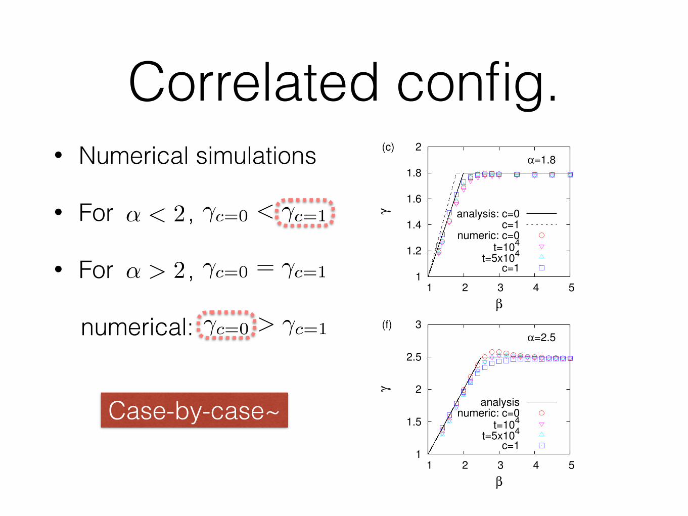
Correlated config.• Numerical simulations

• For ,

• For ,

numerical:

�c=0 = �c=1↵ > 2

�c=0 < �c=1↵ < 2

1

1.2

1.4

1.6

1.8

2

1 2 3 4 5

γ

β

(c)α=1.8

analysis: c=0c=1

numeric: c=0t=104

t=5x104

c=1

1

1.5

2

2.5

3

1 2 3 4 5

γ

β

(f)α=2.5


t=104

t=5x104

c=1

10-8

10-6

10-4

10-2

100

100 101 102 103 104

P(D

)

D

(a)

c=0, α=1.8

γ=1.48

γ=1.8

β=1.61.82.02.43.0

10-8

10-6

10-4

10-2

100

100 101 102 103 104

P(D

)

D

(b)

c=1, α=1.8

γ=1.6

γ=1.8

β=1.61.82.02.43.0

10-10

10-8

10-6

10-4

10-2

100

100 101 102 103 104

P(D

)

D

(d)

c=0, α=2.5

γ=1.6

γ=2.5

β=1.62.02.63.04.0

10-10

10-8

10-6

10-4

10-2

100

100 101 102 103 104

P(D

)

D

(e)

c=1, α=2.5

γ=1.6

γ=2.5

β=1.62.02.63.04.0



��

is due to D =

Pl

n=1

v

n


n



�� ⌘ �

c=1

� �

c=0

=

⇢(2� ↵)(� � 1) if � < ↵,(↵� 1)(2� �) if � > ↵.





Dow

nloa

ded

from

asc

elib

rary

.org

by

Uni

vers

ity o

f Liv

erpo

ol o

n 07

/08/

14. C

opyr

ight

ASC

E. F

or p

erso

nal u

se o

nly;

all

right

s res

erve

d.

�c=0 > �c=1

Case-by-case~

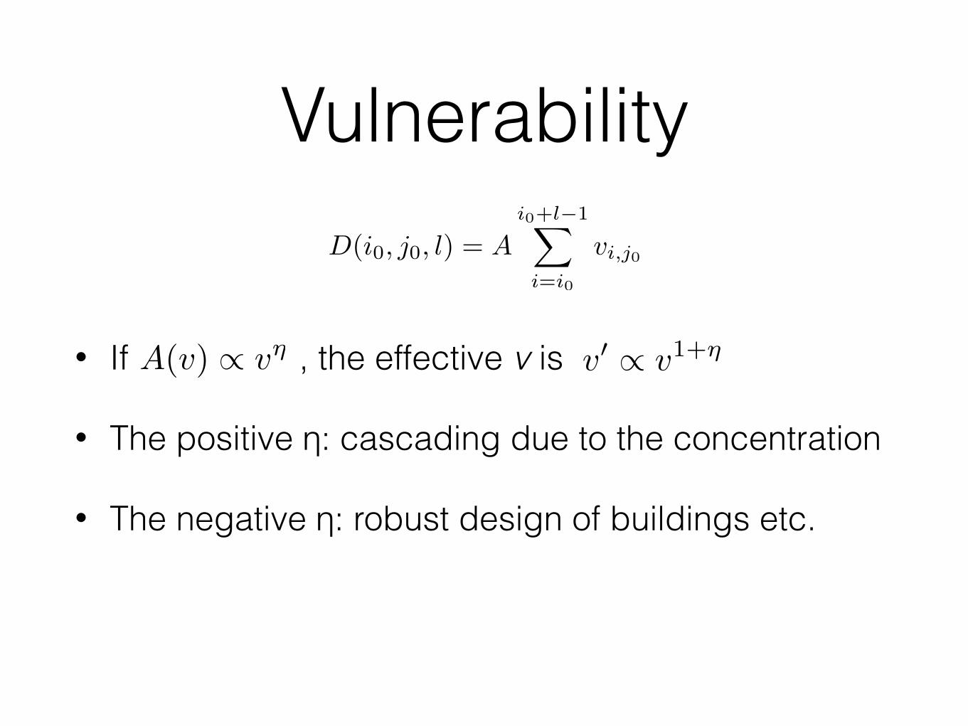
Vulnerability

• If , the effective v is

• The positive η: cascading due to the concentration

• The negative η: robust design of buildings etc.

A(v) / v⌘ v0 / v1+⌘

D(i0, j0, l) = Ai0+l�1X

i=i0

vi,j0

Remarks

• The risk analysis based on the thin-tailed distributions must be improved.

• More realistic simulation and theory?