Optimal multi-configuration approximation of anN -fermion wave function

Jiang-min Zhang

In collaboration with Marcus Kollar

December 12, 2013

Outline

I A basic (but surprisingly overlooked) problem

I How to approximate a given fermionic wave function with Slaterdeterminants

I A simple iterative algorithmI converges monotonically and thus definitelyI easily parallelized

I Some analytic resultsI Mathematically interesting and challenging

I Multi-configuration time-dependent Hartree FockI Spinless fermions in 1D

A Basic Problem

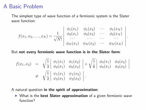
The simplest type of wave function of a fermionic system is the Slaterwave function:

f(x1, x2, . . . , xN ) =1√N !

∣∣∣∣∣∣∣∣φ1(x1) φ1(x2) · · · φ1(xN )φ2(x1) φ2(x2) · · · φ2(xN )· · · · · · · · · · · ·

φN (x1) φN (x2) · · · φN (xN )

∣∣∣∣∣∣∣∣ .But not every fermionic wave function is in the Slater form:

f(x1, x2) =

√1

3

∣∣∣∣ φ1(x1) φ1(x2)φ2(x1) φ2(x2)

∣∣∣∣+√

1

6

∣∣∣∣ φ3(x1) φ3(x2)φ4(x1) φ4(x2)

∣∣∣∣6=

√1

2

∣∣∣∣ ψ1(x1) ψ1(x2)ψ2(x1) ψ2(x2)

∣∣∣∣ .A natural question in the spirit of approximation:

I What is the best Slater approximation of a given fermionic wavefunction?

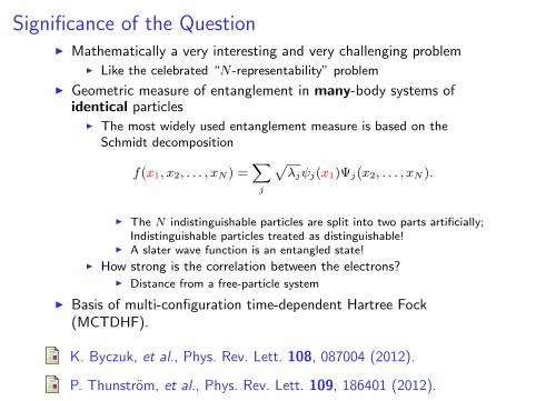
Significance of the QuestionI Mathematically a very interesting and very challenging problem

I Like the celebrated “N -representability” problem

I Geometric measure of entanglement in many-body systems ofidentical particles

I The most widely used entanglement measure is based on theSchmidt decomposition

f(x1, x2, . . . , xN ) =∑j

√λjψj(x1)Ψj(x2, . . . , xN ).

I The N indistinguishable particles are split into two parts artificially;Indistinguishable particles treated as distinguishable!

I A slater wave function is an entangled state!I How strong is the correlation between the electrons?

I Distance from a free-particle system

I Basis of multi-configuration time-dependent Hartree Fock(MCTDHF).

K. Byczuk, et al., Phys. Rev. Lett. 108, 087004 (2012).

P. Thunstrom, et al., Phys. Rev. Lett. 109, 186401 (2012).

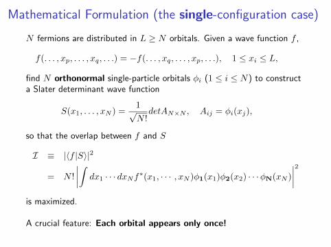
Mathematical Formulation (the single-configuration case)

N fermions are distributed in L ≥ N orbitals. Given a wave function f ,

f(. . . , xp, . . . , xq, . . .) = −f(. . . , xq, . . . , xp, . . .), 1 ≤ xi ≤ L,

find N orthonormal single-particle orbitals φi (1 ≤ i ≤ N) to constructa Slater determinant wave function

S(x1, . . . , xN ) =1√N !

detAN×N , Aij = φi(xj),

so that the overlap between f and S

I ≡ |〈f |S〉|2

= N !

∣∣∣∣∫ dx1 · · · dxNf∗(x1, · · · , xN )φ1(x1)φ2(x2) · · ·φN(xN )

∣∣∣∣2is maximized.

A crucial feature: Each orbital appears only once!

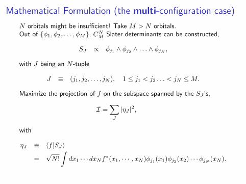
Mathematical Formulation (the multi-configuration case)

N orbitals might be insufficient! Take M > N orbitals.Out of {φ1, φ2, . . . , φM}, CNM Slater determinants can be constructed,

SJ ∝ φj1 ∧ φj2 ∧ . . . ∧ φjN ,

with J being an N -tuple

J ≡ (j1, j2, . . . , jN ), 1 ≤ j1 < j2 . . . < jN ≤M.

Maximize the projection of f on the subspace spanned by the SJ ’s,

I =∑J

|ηJ |2,

with

ηJ ≡ 〈f |SJ〉

=√N !

∫dx1 · · · dxNf∗(x1, · · · , xN )φj1(x1)φj2(x2) · · ·φjN (xN ).

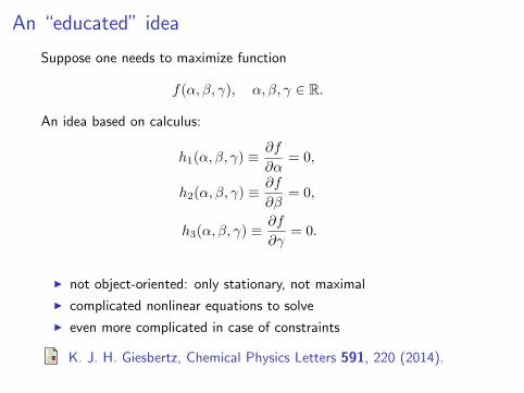
An “educated” idea

Suppose one needs to maximize function

f(α, β, γ), α, β, γ ∈ R.

An idea based on calculus:

h1(α, β, γ) ≡∂f

∂α= 0,

h2(α, β, γ) ≡∂f

∂β= 0,

h3(α, β, γ) ≡∂f

∂γ= 0.

I not object-oriented: only stationary, not maximal

I complicated nonlinear equations to solve

I even more complicated in case of constraints

K. J. H. Giesbertz, Chemical Physics Letters 591, 220 (2014).

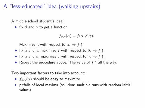
A “less-educated” idea (walking upstairs)

A middle-school student’s idea:

I fix β and γ to get a function

fβ,γ(α) ≡ f(α, β, γ).

Maximize it with respect to α. ⇒ f ↑.I fix α and γ, maximize f with respect to β. ⇒ f ↑.I fix α and β, maximize f with respect to γ. ⇒ f ↑.I Repeat the procedure above. The value of f ↑ all the way.

Two important factors to take into account:

I fβ,γ(α) should be easy to maximize

I pitfalls of local maxima (solution: multiple runs with random initialvalues)

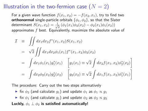
Illustration in the two-fermion case (N = 2)

For a given wave function f(x1, x2) = −f(x2, x1), try to find twoorthonormal single-particle orbitals {φ1, φ2}, so that the Slaterdeterminant S(x1, x2) =

1√2(φ1(x1)φ2(x2)− φ2(x1)φ1(x2))

approximates f best. Equivalently, maximize the absolute value of

I ≡∫∫

dx1dx2f∗(x1, x2)S(x1, x2)

=√2

∫∫dx1dx2φ1(x1)f

∗(x1, x2)φ2(x2)

=

∫dx1φ1(x1)g

∗1(x1)

[g1(x1) ≡

√2

∫dx2f(x1, x2)φ

∗2(x2)

]=

∫dx2φ2(x2)g

∗2(x2)

[g2(x2) ≡

√2

∫dx1f(x1, x2)φ

∗1(x1)

]The procedure: Carry out the two steps alternatively

I fix φ2 (and calculate g1) and update φ1 as φ1 ∝ g1I fix φ1 (and calculate g1) and update φ2 as φ2 ∝ g2

Luckly, φ1 ⊥ φ2 is satisfied automatically!

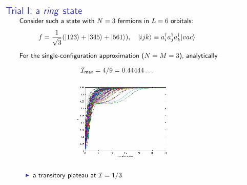
Trial I: a ring stateConsider such a state with N = 3 fermions in L = 6 orbitals:

f =1√3(|123〉+ |345〉+ |561〉), |ijk〉 ≡ a†ia

†ja†k|vac〉

For the single-configuration approximation (N =M = 3), analytically

Imax = 4/9 = 0.44444 . . .

I a transitory plateau at I = 1/3

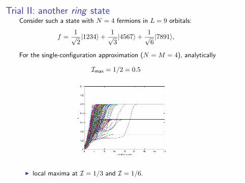
Trial II: another ring stateConsider such a state with N = 4 fermions in L = 9 orbitals:

f =1√2|1234〉+ 1√

3|4567〉+ 1√

6|7891〉,

For the single-configuration approximation (N =M = 4), analytically

Imax = 1/2 = 0.5

I local maxima at I = 1/3 and I = 1/6.

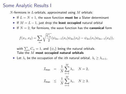
Some Analytic Results I

N -fermions in L-orbitals, approximated using M orbitals:

I If L = N + 1, the wave function must be a Slater determinant

I If M = L− 1, just drop the least occupied natural orbital

I If N = 2, for fermions, the wave function has the canonical form

f(x1, x2) =∑α

√Cα2

(ψ2α−1(x1)ψ2α(x2)− ψ2α(x1)ψ2α−1(x2)),

with∑α Cα = 1, and {ψi} being the natural orbitals.

Take the M most occupied natural orbitals

I Let λi be the occupation of the ith natural orbital, λi ≥ λi+1,

Imax =1

N

M∑i=1

λi, N = 2,

Imax ≤ 1

N

M∑i=1

λi, N ≥ 3.

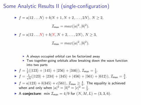
Some Analytic Results II (single-configuration)

I f = a|12 . . . N〉+ b|N + 1, N + 2, . . . , 2N〉, N ≥ 2,

Imax = max(|a|2, |b|2).

I f = a|12 . . . N〉+ b|N,N + 2, . . . , 2N〉, N ≥ 3,

Imax = max(|a|2, |b|2).

I A always occupied orbital can be factorized awayI Two together-going orbitals allow breaking down the wave function

into two parts

I f = 12 (|123〉+ |145〉+ |256〉+ |346〉), Imax = 1

2 .

I f = 1√6(|123〉+ |234〉+ |345〉+ |456〉+ |561〉+ |612〉), Imax = 3

4 .

I f = a|123〉+ b|345〉+ c|561〉, Imax ≥ 49 . The equality is achieved

when and only when |a|2 = |b|2 = |c|2 = 13 .

I A conjecture: min Imax = 4/9 for (N,M,L) = (3, 3, 6).

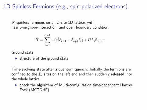
1D Spinless Fermions (e.g., spin-polarized electrons)

N spinless fermions on an L-site 1D lattice, withnearly-neighbor-interaction, and open boundary condition,

H =

L−1∑i=1

−(c†i ci+1 + c†i+1ci) + Unini+1.

Ground state

I structure of the ground state

Time-evolving state after a quantum quench: Initially the fermions areconfined to the Li sites on the left end and then suddenly released intothe whole lattice.

I check the algorithm of Multi-configuration time-dependent HartreeFock (MCTDHF)

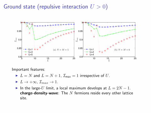
Ground state (repulsive interaction U > 0)

5 10 15 20 250.8

0.85

0.9

0.95

1

L

Imax

(a) N = M = 5U=1

U=3

U=5

10 15 20 250.8

0.85

0.9

0.95

1

L

Imax

(b) N = M = 6U=1

U=2

U=4

Important features:

I L = N and L = N + 1, Imax = 1 irrespective of U .

I L→ +∞, Imax → 1.

I In the large-U limit, a local maximum develops at L = 2N − 1.charge-density-wave: The N fermions reside every other latticesite.

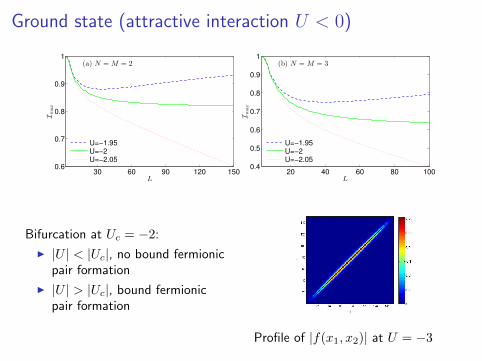
Ground state (attractive interaction U < 0)

30 60 90 120 1500.6

0.7

0.8

0.9

1

L

Imax

(a) N = M = 2

U=−1.95

U=−2

U=−2.05

20 40 60 80 1000.4

0.5

0.6

0.7

0.8

0.9

1

L

Imax

(b) N = M = 3

U=−1.95

U=−2

U=−2.05

Bifurcation at Uc = −2:

I |U | < |Uc|, no bound fermionicpair formation

I |U | > |Uc|, bound fermionicpair formation

Profile of |f(x1, x2)| at U = −3

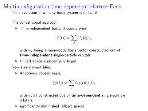
Multi-configuration time-dependent Hartree FockTime evolution of a many-body system is difficult!

The conventional approach:

I Time-independent basis, chosen a priori

|ψ(t)〉 =∑J

CJ(t)eJ ,

with eJ being a many-body basis vector constructed out oftime-independent single-particle orbitals.

I Hilbert space exponentially large!

Now a very smart idea:

I Adaptively chosen basis,

|ψ(t)〉 '∑J

CJ(t)eJ(t),

with eJ(t) constructed out of time-dependent single-particleorbitals.

I significantly diminished Hilbert space!

Multi-configuration time-dependent Hartree Fock

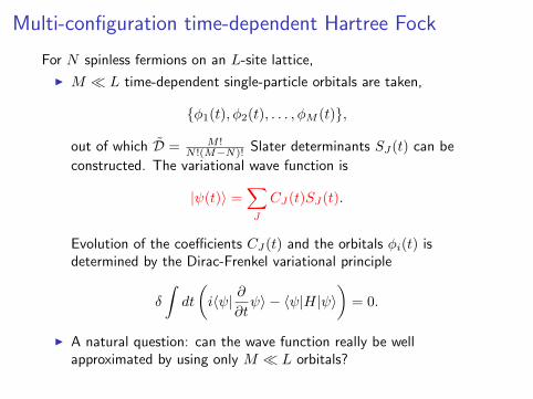
For N spinless fermions on an L-site lattice,

I M � L time-dependent single-particle orbitals are taken,

{φ1(t), φ2(t), . . . , φM (t)},

out of which D = M !N !(M−N)! Slater determinants SJ(t) can be

constructed. The variational wave function is

|ψ(t)〉 =∑J

CJ(t)SJ(t).

Evolution of the coefficients CJ(t) and the orbitals φi(t) isdetermined by the Dirac-Frenkel variational principle

δ

∫dt

(i〈ψ| ∂

∂tψ〉 − 〈ψ|H|ψ〉

)= 0.

I A natural question: can the wave function really be wellapproximated by using only M � L orbitals?

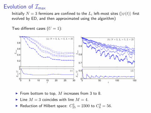
Evolution of Imax

Initially N = 3 fermions are confined to the Li left-most sites (|ψ(t)〉 firstevolved by ED, and then approximated using the algorithm)

Two different cases (U = 1):

0

0.2

0.4

0.6

0.8

1

Imax

(a) N = 3, Li = 3, L = 25

0 5 10 15 20 25 300

1

2

t

Eint/U (c)

0.7

0.8

0.9

1

Imax

(b) N = 3, Li = 5, L = 25

0 50 100 1500

0.5

t

Eint/U (d)

I From bottom to top, M increases from 3 to 8.

I Line M = 3 coincides with line M = 4.

I Reduction of Hilbert space: C325 = 2300 to C3

8 = 56.

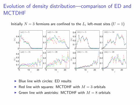
Evolution of density distribution—comparison of ED andMCTDHF

Initially N = 3 fermions are confined to the Li left-most sites (U = 1)

0

0.2

0.4

〈ni〉

(a1) t = 5

0

0.1

0.2

(a2) t = 10

0 10 200

0.1

0.2

0.3

0.4

i

〈ni〉

(a3) t = 15

0 10 200

0.1

0.2

0.3

i

(a4) t = 20

0

0.1

0.2

0.3

0.4

〈ni〉

(b1) t = 5

0

0.1

0.2

(b2) t = 10

0 10 200

0.2

0.4

0.6

i〈n

i〉

(b3) t = 15

0 10 200

0.1

0.2

0.3

i

(b4) t = 20

I Blue line with circles: ED results

I Red line with squares: MCTDHF with M = 3 orbitals

I Green line with aestrisks: MCTDHF with M = 8 orbitals

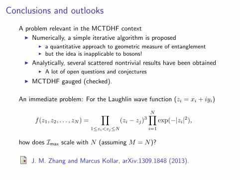
Conclusions and outlooks

A problem relevant in the MCTDHF context

I Numerically, a simple iterative algorithm is proposedI a quantitative approach to geometric measure of entanglementI but the idea is inapplicable to bosons!

I Analytically, several scattered nontrivial results have been obtainedI A lot of open questions and conjectures

I MCTDHF gauged (checked).

An immediate problem: For the Laughlin wave function (zi = xi + iyi)

f(z1, z2, . . . , zN ) =∏

1≤zi<zj≤N

(zi − zj)3N∏i=1

exp(−|zi|2),

how does Imax scale with N (assuming M = N)?

J. M. Zhang and Marcus Kollar, arXiv:1309.1848 (2013).