GRASSLAND ECOSYSTEM

Methods of Vegetation Analysis Through the use of Plot sampling

_______________

A Scientific Paper

Presented to:

Liza A. Adamat, Ph.D.

Department of Biological Sciences

CSM, MSU – IIT

_______________

Presented by:

Shaina Mavreen D. Villaroza

In Partial Fulfillment of the course Bio 107.2 General Ecology

Second Semester 2014-2015

1

ACKNOWLEDGEMENT

Apart from the effort I have done, the success of this field sampling depends

largely on the encouragement and guidelines of many others. I take this opportunity to

express my gratitude to the people who have been instrumental in this successful

sampling. I would like to show my greatest appreciation to Prof. Liza Adamat for the

guidance and help. Without the guidance, this sampling would not have been successful.

2

ABSTRACT

Grassland is entirely composed of tall grasses and lacks trees to grow because

of its scarcity in water. It is maintained by fire to improve the poor quality in it and is an

important natural component of many grassland communities. The purpose of the study is

to determine the cover and density estimates, the species-area curve and the density of

plant species in a grassland ecosystem. With the use of quadrats for plot sampling and the

transect line for transect sampling method, results were determined. Different set-up was

conducted to obtain a certain result. Quadrat and Transect line were entirely used in this

experiment. A 10-m transect line was laid and the 1 square meter quadrat was put at the

end of the 10m transect line and number of species were counted. Results show that in

the tabulation for the species-area curve, the number of species found increases as the

area examined increases. For the estimation of top cover of grasses in the quadrat, varied

percentages were recorded when using different methods of estimation but more or less

follows the same pattern in showing which species are more abundant than the other.

Density estimation, along with Dominance, Frequency, and Importance Value were also

computed for each grass species found in the quadrat. The species richness during the

conduction of Zonation and Density Estimation was 8 and the computed Diversity Index

(Simpson’s Index) value is 0.1932 which implies that the species in the grassland

community is diverse.

3

INTRODUCTION

Grassland characterizes as terrestrial ecosystem in which grasses dominates in

it rather than the large shrubs or trees. This area is entirely compose of tall grasses and is

too dry for many trees to grow and is maintain by fire. One of the simplest and least

expensive practices to improve poor quality grassland is burning. Research within the

past few decades show that fire is an important natural component of many grassland

communities (Daubenmire, 1968). It allows the plant to reach water quickly and makes

the plant particularly resistant to fire. Because of the open landscape and widely spread

trees, grasslands are home to large herds of grazing mammals. Species use to live in it

because of its richness in grasses that are dominant in grassland. It is characterizing by

mix herbaceous (nonwoody) vegetation cover and is composed of different individuals of

plant species.

The objectives of this experiment are to train the students on the principles of

plot and transect sampling as applied in ecological research, to construct a zonation of

diagram of a grassland ecosystem, to be able to interpret the implication of different

combined parameters and to determine the cover and density estimates, the species area

curve and the density of plant species in a grassland ecosystem.

In determining its area, one of the most effective methods of vegetation

analysis is through the use of Plot sampling. This method is use for obtaining samples of

both terrestrial and aquatic such as the plants and slow moving organisms. Quadrat size

depends to a large extent on the type of survey being conducted. As a general guideline,

0.5-1.0 square meter quadrats would be suggested for short grassland. Quadrats ranging

from 0.5 to 2.0 square meters are suggested for grassland vegetation.

4

MATERIALS AND METHODS

This fieldwork sampling was conducted at New Frontier Court, Santiago,

Iligan City (Figure 1). Plot sampling method was entirely used in this study area with the

square meter quadrat, tape measure and the transect line.

Figure 1. Location of the sampling site.

In preparing the Species area curve, only 1 square meter quadrat was used

and positioned in the area that has been selected randomly to be sampled in. Plant species

present in the smallest quadrat that is 10 cm x 10 cm within the 1 square meter quadrat

was counted and being recorded. The smallest subquadrat was being doubled and the

number of species in this new area was observed and recorded. The step in which the

smallest subquadrat was doubled and counted has been repeated until the number of

species counted at each doubled subquadrat size gave no new species. In obtaining the

species area curve, the number of species against the quadrat size was plotted.

5

In obtaining the Cover estimation of vegetation, the area covered with

grasses in the 1 square meter quadrat was estimated and being recorded. The cover of

estimation of vegetation was categorized into direct estimation top cover, Subquadrat

estimation of top cover, 50% method, Braun-Blanquet 5 point scale and the Domin scale.

In the direct estimation, the top cover for the whole quadrat was visually

estimated and each species was recorded to the nearest percent. Thus, the total for all

species and bare ground will be equaled to 100%.

The Subquadrat estimation of top cover was computed as the sum of the

results in the 25 of the 100 10cm x 10 cm subquadrat, that is, every fourth quadrat. In

obtaining the estimate of cover percentages for the 1 square meter quadrat, the mean of

the sum of the results was calculated and recorded.

The 50% method was obtained in the 100 subquadrats. Species in the

quadrat occupies greater than or equal to 50%. In this method, the summed values often

lie below 100% since many subquadrats will contain a species mixed where no single

species or bare ground will reach 50%.

In the Braun-Blanquet 5 point scale, the cover of each species and bare

ground for the square meter plot was visually estimated using the following scale:

+ Very rare less than 1%1 rare 1-5%2 occasional 6-25%3 frequent 26-50%4 common 51-75%5 abundant 76-100%

In the Domin scale, visually estimate the cover of each species for the 1 square meter plot using the following scale:

+ A single individual 1 Scarce, 1-2 individual2 Very scattered, cover small, less than 1%3 Scattered, cover small 1-4%4 Abundant, cover 5-10%

6

5 Abundant, cover 11-25%6 Abundant, cover 26-33%7 Abundant, cover 34-50%8 Abundant, cover 51-75%9 Abundant, cover greater than 75% but not complete10 Cover practically complete

In determining the Zonation and Density estimation, the calibrated 10 m

transect line was laid down across the study area by connecting two randomly selected

points. Transect line must be at least 5m distance from those of other groups. The number

of plants intercepted by the transect line were counted and identified. Begin at one end of

the line. It included those plants whose Arial foliage overlies the transect line and those

that are touched by the line or intercepted within a 1 cm strip of the line. The distance

intercepted by each plant in the line was measured with the use of the Tape measure. In

making the Zonation diagram, brackets were used to indicate the intercepted distance.

Plant height, type of substrate and depth of standing water if present, may also be noted.

Also, the side and top view images must be illustrated.

In the setup of a 100m transect line on the study area, two 10m transects per

group will be put up and placed a 1 square meter quadrat at the end of the 10m transect

line and the number of species then is being counted. Reposition the quadrat at the end of

the next transects line and estimate the number of species at each new position. There

will be a total of 10 samplings units or quadrats for the entire study area. Thus, sampling

size will be 100 square meter. Zonation and Density estimation can be computed by the

following formula:

Density of a species = No. of individuals of a species Total area sampled

Relative Density = Density of a species x 100 Total density of all species

Dominance of a species = Total area covered by a speciesTotal area sampled

Relative Dominance = Dominance of a species x 100 Total dominance of all species

7

Frequency of a species = No. of quadrats where a species occursRelative Frequency = Frequency value for a species x 100

Total frequency of all species

Importance value = relative density + relative dominance + relative frequency

In determining diversity measurements, the Simpson’s and Shannon Weiner’s

indices for measuring diversity can be used and computed using the data from different

sampling techniques on the species composition and number of individuals for species.

8

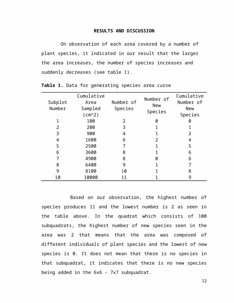
RESULTS AND DISCUSSION

On observation of each area covered by a number of plant species, it indicated in

our result that the larger the area increases, the number of species increases and suddenly

decreases (see table 1).

Table 1. Data for generating species area curve

Subplot Number

Cumulative Area Sampled

(cm^2)

Number of Species

Number of New Species

Cumulative Number of

New Species1 100 2 0 02 200 3 1 13 900 4 1 24 1600 6 2 45 2500 7 1 56 3600 8 1 67 4900 8 0 68 6400 9 1 79 8100 10 1 810 10000 11 1 9

Based on our observation, the highest number of species produces 11 and the

lowest number is 2 as seen in the table above. In the quadrat which consists of 100

subquadrats, the highest number of new species seen in the area was 2 that means that the

area was composed of different individuals of plant species and the lowest of new species

is 0. It does not mean that there is no species in that subquadrat, it indicates that there is

no new species being added in the 6x6 - 7x7 subquadrat.

9

0 2000 4000 6000 8000 10000 120000

2

4

6

8

10

12

species

Area (cm^2)

Num

ber o

f Spe

cies

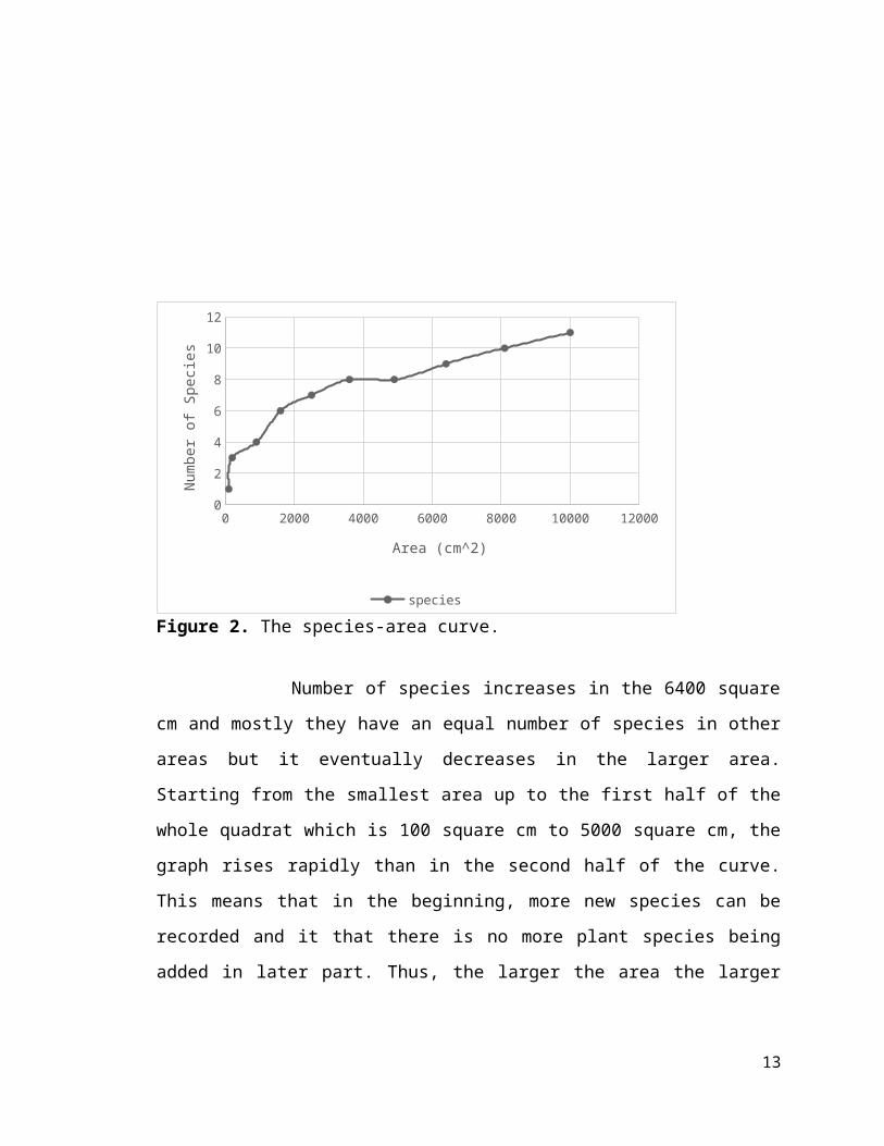
Figure 2. The species-area curve.

Number of species increases in the 6400 square cm and mostly they have an

equal number of species in other areas but it eventually decreases in the larger area.

Starting from the smallest area up to the first half of the whole quadrat which is 100

square cm to 5000 square cm, the graph rises rapidly than in the second half of the curve.

This means that in the beginning, more new species can be recorded and it that there is no

more plant species being added in later part. Thus, the larger the area the larger number

of species occurred in it but then suddenly decreases.

On the estimation of top cover in quadrat no. 1, it resulted that Species A has

the highest value estimated compared to that in the Species B (see Table 2).

Table 2.Estimation of top cover in quadrat no.1

Species Direct Estimation

SubquadratEstimation

50% Method

Braun - Blanquet

Domin Scale

1 40% 45% 40% 5 92345

30%20%5%5%

30%15%5%5%

25%25%5%5%

5432

8654

10

In the above table, it can be inferred that Species 1 had dominated the area

being conducted in the sample compared to the other species 2-5. Species 1 was abundant

in the area than the rest of the species from 2-5.

On observation of the tabulation of raw data for density estimation, it

resulted that Quadrat number 1 has richer species with eight species recorded while

Quadrat number 2 only had three species but with greater count of individuals included in

the quadrat (see Table 3).

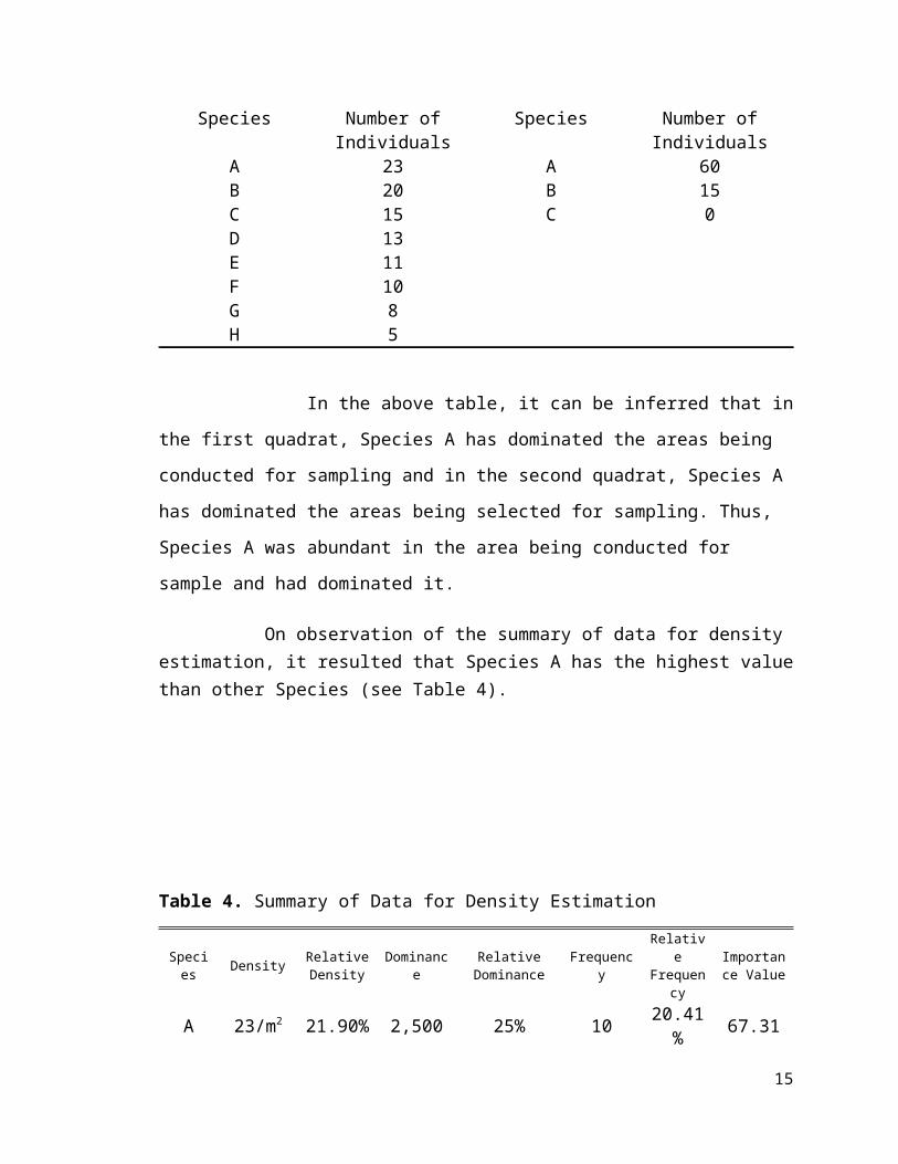
Table 3.Tabulation of Raw Data for Density Estimation

Quadrat no.1 Quadrat no. 2Species Number of

IndividualsSpecies Number of

IndividualsA 23 A 60B 20 B 15CDEFGH

1513111085

C 0

In the above table, it can be inferred that in the first quadrat, Species A has

dominated the areas being conducted for sampling and in the second quadrat, Species A

has dominated the areas being selected for sampling. Thus, Species A was abundant in

the area being conducted for sample and had dominated it.

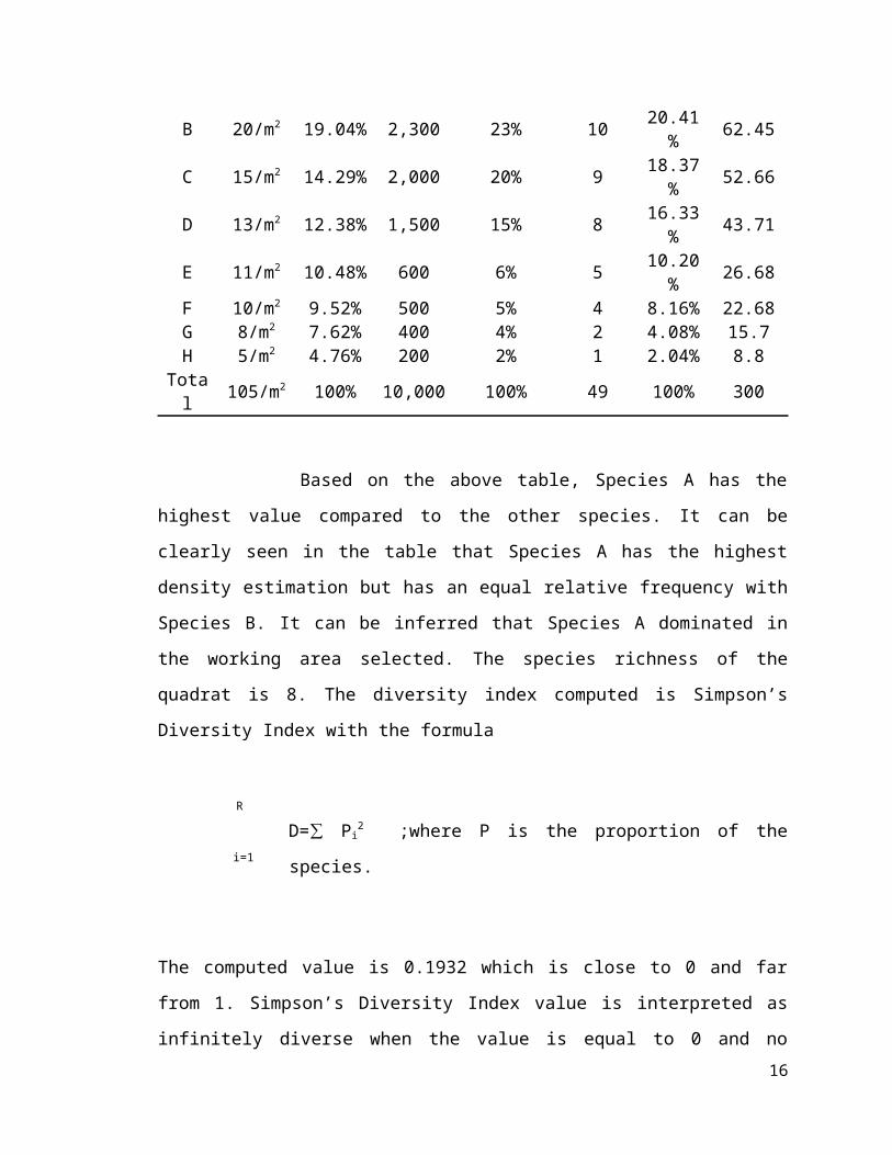
On observation of the summary of data for density estimation, it resulted that Species A has the highest value than other Species (see Table 4).

Table 4. Summary of Data for Density Estimation

Species Density Relative Dominance Relative Frequency Relative Importance

11

Density Dominance Frequency Value

A 23/m2 21.90% 2,500 25% 10 20.41% 67.31B 20/m2 19.04% 2,300 23% 10 20.41% 62.45C 15/m2 14.29% 2,000 20% 9 18.37% 52.66D 13/m2 12.38% 1,500 15% 8 16.33% 43.71E 11/m2 10.48% 600 6% 5 10.20% 26.68F 10/m2 9.52% 500 5% 4 8.16% 22.68G 8/m2 7.62% 400 4% 2 4.08% 15.7H 5/m2 4.76% 200 2% 1 2.04% 8.8

Total 105/m2 100% 10,000 100% 49 100% 300

Based on the above table, Species A has the highest value compared to the

other species. It can be clearly seen in the table that Species A has the highest density

estimation but has an equal relative frequency with Species B. It can be inferred that

Species A dominated in the working area selected. The species richness of the quadrat is

8. The diversity index computed is Simpson’s Diversity Index with the formula

D=∑ Pi2 ;where P is the proportion of the species.

The computed value is 0.1932 which is close to 0 and far from 1. Simpson’s Diversity

Index value is interpreted as infinitely diverse when the value is equal to 0 and no

diversity when the value is equal to 1. The result tells us that there is a diverse species of

plant species in the grassland.

12

R

i=1

CONCLUSION

This report introduces two methods which are Plot sampling and the Transect

sampling method. The species-area curve, the cover and density of plant species in a

grassland ecosystem conducted were determined with the use of quadrats and the transect

line as well as the top cover estimation methods. Based on the results, the number of

species present in the area being conducted ranges from 2-11. It can be inferred that the

larger the area, the larger number of species will occur in that area but then eventually

decreases. It can be that there is no more plant species added in the said area. In the

estimation of top cover and the tabulation of raw data for density estimation, it can be

inferred that Species A had dominated the area being conducted compared to that of the

other species found within the qaudrat. Thus, species A was abundant in the area being

conducted and selected and had dominated it. Species A also had the greatest Importance

Value which could mean of it being the keystone species in the grassland ecosystem.

13

REFERENCES

Daubenmire, R.F. 1968. Grassland ecosystem

Grassland Ecosystem. 2002. Retrieved on March 11, 2015. http://encyclopedia2. The freedictionary.com/Grassland + Ecosystem

McGraw-Hill concise Encyclopedia of Bioscience ©2002 by the McGraw-HillCompanies, Inc.

14

COASTAL MARINE ECOSYSTEM

Assessment of Macrobenthic Flora and Fauna in the Intertidal Area

_______________

A Scientific Paper

Presented to:

Liza A. Adamat, Ph.D.

Department of Biological Sciences

CSM, MSU – IIT

_______________

Presented by:

Shaina Mavreen D. Villaroza

In Partial Fulfillment of the course Bio 107.2 General Ecology

Second Semester 2014-2015

15

ABSTRACT

Philippines has a vast territory of marine coastal water and people get their livelihood

from the abundance of the resources provided by the coastal marine ecosystem. This

ecosystem is greatly affected by many factors and any damage to it could affect the

country’s economy and therefore, people must be aware of its importance as well as

understand different methods to assess coastal bioresources to gain more knowledge

regarding its conservation. The objectives of the study is to assess the macrobenthic flora

and fauna species to correlate the relative abundance of the flora and fauna to the

physico-chemical paramaters, and to determine the ecological indices of the area. It is

hypothetical to expect the presence of macrobenthic flora and fauna in an area with good

and normal physic-chemical parameters. The study was done with the use of Quadrat and

Transect method. A 1x1m steel quadrat was laid along the calibrated transect line in

every 10 meters and algae and seagrass individuals within the quadrat were counted.

Specimen sample was collected for documentation and indentification. The physico-

chemical parameters were measured with three repeated trials using a thermometer for

the water and soil temperature, improvised psychrometer for humidity, and pH paper for

the pH. Sediment grain size analysis was conducted. Results show that there is only one

species of green algae (Chlorophyta) that was found in the area. Macrobenthic fauna is

also absent. Physico-chemical parameters were at a normal range. However, the sampling

site was located in a seaport near Mabuhay Vinyl Corporation (MVC) and the beach was

also inhabited by the locals. This means that the area is disturbed and unprotected which

makes it inhabitable for algae and especially for seagrasses.

16

INTRODUCTION

Marine ecosystem are among the largest of Earth's aquatic ecosystem. They

include oceans, salt marshes, intertidal zones, estuaries, lagoons, mangrove, coral reefs,

the deep sea, and the sea floor. They can be constrasted with freshwater considered

ecosystems because the land life support the animal life and vice-versa. According to

Finke et al. (2007), marine ecosystem usually have a large biodiversity and are therefore

thought to have a good resistance against invasive species. However, exceptions have

been observed, and the mechanisms responsible in determining the success of an invasion

are not yet clean.

Coastal marine ecosystem are severely threatened by climate change due to

changes in sea level, storm and wave regimes, flooding, altered sediment budgets and the

loss of coastal habitat ( Harley et al. 2006; Jones, Gladstone & Hacking 2007). In the

intertidal Area, it has macrobenthic flora and fauna zonation pattern (McLachlan &

Jaramillo 1995) concluded that macrofauna and flora distribution across shore assumes

the form of three distinct and universal zones level on the distribution of characteristics

taxa.

Marine environment can be characterized broadly as a water, pelagic,

environment and a bottom, or benthic environment. Within the pelagic environment the

water are divided into the neritic province, which includes the water above continental

shelf, and the oceanic province which includes all the open waters beyond the continental

self.

17

The aim of this study is to determine the composition and relative abundance of

macrobenthic flora ( red, green, brown algae and seagrass), composition and relative

abundance of different macrobenthic faunal species, sediment type in each sampling area,

correlation between relative abundance of the flora and fauna to the physico-chemical

parameters and ecological indeces ( Index of dominance, similarity, evenness, and

diversity).

18

MATERIALS AND METHODS

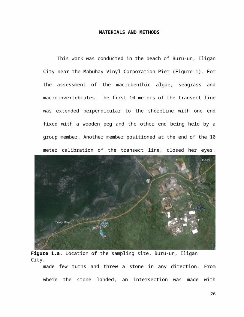
This work was conducted in the beach of Buru-un, Iligan City near the Mabuhay

Vinyl Corporation Pier (Figure 1). For the assessment of the macrobenthic algae, seagrass

and macroinvertebrates. The first 10 meters of the transect line was extended

perpendicular to the shoreline with one end fixed with a wooden peg and the other end

being held by a group member. Another member positioned at the end of the 10 meter

calibration of the transect line, closed her eyes, made few turns and threw a stone in any

direction. From where the stone landed, an intersection was made with another rope to

the 10 meter transect line and the 1x1 meter square steel quadrat was thrown near the

intersection aligned with the 10-meter transect line (Figure 2.)

19

Figure 1.a. Location of the sampling site, Buru-un, Iligan City.

20

The number of squares with a particular algal group (red, green, or brown) and

seagrasses were counted. Observations were recorded in a field notebook. Small

21

Figure 3.b. View of Mabuhay Vinyl Corporation (MVC) seaport from Timoga, Iligan City.

Figure 4. Representation in aerial view of the setting up of quadrat and transect for the assessment proper.

representative samples were collected for every species of each algal group for

documentation. The collected specimen was placed in a plastic bag with adequate

seawater to immerse the specimen.

The physico-chemical parameters of the coastal marine ecosystem were

determined. Three readings for each parameter were recorded including the Soil and

Water Temperature, Humidity, and pH using a thermometer, improvised psychrometer,

and pH paper respectively. Sediment grain size analysis was also conducted.

22

RESULTS AND DISCUSSION

The sampling area is a disturbed area since it is located near a pier of the

Mabuhay Vinyl Corporation seaport. The shore was also lined up with local residents

making the area unprotected and aggravated. This can be correlated with the findings

after the assessment of the macrobenthic flora and fauna in the intertidal area shown in

the following tables.

Table 1.1 Relative abundance of macrobenthic flora.

Quadrat Number Number of squares Percentage Relative Abundance10 1 1% 100%20 0 0% 0%30 0 0% 0%40 0 0% 0%50 0 0% 0%60 0 0% 0%70 0 0% 0%80 0 0% 0%

Table 1.1 indicates the number of macrobenthic flora on a certain corresponding

quadrat number and it shows that only the first quadrat with only one subquadrat covered

any macrobenthic flora. The relative abundance is 100% since there are no other species

found for it to be compared with.

23

Table 1.2 Relative abundance of macrobenthic fauna.

Quadrat Number Animal Species Count Relative Abundance

10 0 0 0

20 0 0 030 0 0 040 0 0 050 0 0 060 0 0 070 0 0 0

On the other hand, Table 1.2 shows total absence of macrobenthic fauna. There

were absolutely no crabs, sea stars, fishes, or others found within the quadrat. This makes

the diversity and species richness of the area extremely low or zero.

Table 1.3 Physico-chemical parameters

Quadrat Number

Temperature(oC)

HumiditySediment

TypepH

Water Soil10 27 25 26 Sand 730 26 26 26 Sand 760 27 25 26 Sand 790 27 25 26 Sand 7

Table 1.3 shows the different physico-chemical parameters such as Temperature,

Humidity, Sediment Type, and pH. These parameters were obtained based on the quadrat

number 10, 30, 60 and 90. The water temperature ranges from 26-27 oC while the soil

temperature is at 25-26 oC. Humdity is generally the same around the area, as well as the

sediment type and pH. These values indicate a normal water condition. However, there is

scarcity of the macrobenthic flora and fauna in the area.

24

Table 1.4 Summary Table of the Macrobenthic flora.

Quadrat Number Chlorophyta Phaeophyta Rhodophta SeagrassCount / Relative

AbundanceCount / Relative

AbundanceCount / Relative

Abundance

Count / Relative

Abundance10 1/100% 0 / 0% 0 / 0% 0 / 0%20 0 / 0% 0 / 0% 0 / 0% 0 / 0%30 0 / 0% 0 / 0% 0 / 0% 0 / 0%40 0 / 0% 0 / 0% 0 / 0% 0 / 0%50 0 / 0% 0 / 0% 0 / 0% 0 / 0%60 0 / 0% 0 / 0% 0 / 0% 0 / 0%70 0 / 0% 0 / 0% 0 / 0% 0 / 0%

Only one individual of the Chlorophyta species or the green algae was found the

area. Red and brown algae as well as seagrasses were absent. Seagrasses are indicators of

the health of a body of water. Their presence means that a body of water is not polluted

and not disturbed. Seagrasses and algae are primary producers in the marine ecosystem.

They form organic food molecules from carbon dioxide and water through

photosynthesis. Any damage to the primary producers can cause imbalance in the entire

marine ecosystem. The absence of these primary producers could be the cause of the

absence of the macrobenthic fauna in the area.

Table 1.5 Ecological Indices of each Stations.

Ecological Indices

Station 1 Station 2 Station 3 Station 4 Station 5

Diversity NA NA NA NA NASimilarity NA NA NA NA NAEvenness NA NA NA NA NA

Dominance NA NA NA NA NA

Ecological indices cannot be analyzed since only one species was found in the entire activity.

25

CONCLUSION

The general condition of the area has many different factors such as the physico-

chemical parameters (temperature, salinity, pH, humidity, organic matter, etc), weather,

altitude, and others. However, the health of a body of water doesn’t only depend on such

factors mentioned. Otherwise, it can be expected that since the sampling area had normal

physic-chemical parameters, plant and animal species must be present. The results

showed clearly the opposite. There can be correlation between physico-chemical factors

and the relative abundance such that if physico-chemical measurements fall in a normal

range for the plants and animals to thrive in, then plants and animals can live in a

particular area. Albeit, other factors such as pollution, disturbance or aggravation,

overfishing, eutrophication, climate change, and other human and natural impacts must

be taken into account in determining the total and general condition of a body of water.

However, this is outside of the scope and limitation of the study conducted, and it can be

advised for further examiners to consider such factors in the assessment of the coastal

marine ecosystem.

26

REFERENCES

Aranico, E., Dagoc, KM., Jimenez, B., Mag-aso, A., Responte, J.A, Tampus, A. (2004). General

Biology,. Laboratory and Field Manual in Bio. 107.2; p.65-67. Mindanao State

University-Iligan Institute of Technology, College of Science and Mathematics,

Department of Biological Science; Iligan City

Finke GR, Navarrete SA, Bozinovic F (2007) Tidal kegiro of temperate coasts and their

influences in

aerial exposure for intertidal organisms Marine Ecology Progress Series, 34.3; 57-62

Harley, C.D.G, Randall Hughes, A, Hultgren, K.M., Miner, B.G, Sorte, C.J.B., Thornber, C.S.,

Rodriguez, L.F., Tomek, L. Z. Williams, S, L. (2006). The impacts of climate change in

coastal marine ecosystems. Ecology Lotters, 9, 228-241.

Jones, A. R., Gladstone, W. & Hacking, N.J. (2007) Australian sandy-beach ecosystems and

climate

change: ecology and management Australian Zoologist, 34, 190-201.

McLachlan, A. & Jaramillo E. 1995. Zonation on sandy beaches; oceanorgr. Mar . Biol, a arev.

33:395-335

http: //en.wikipedia.org/wiki/Marine_ecosystem

27