Embed Size (px)
Citation preview
Scaling structured predictionTommi Jaakkola
MIT
in collaboration withM. Collins, M. Fromer, T. Hazan, T. Koo,
O. Meshi, A. Rush, D. Sontag
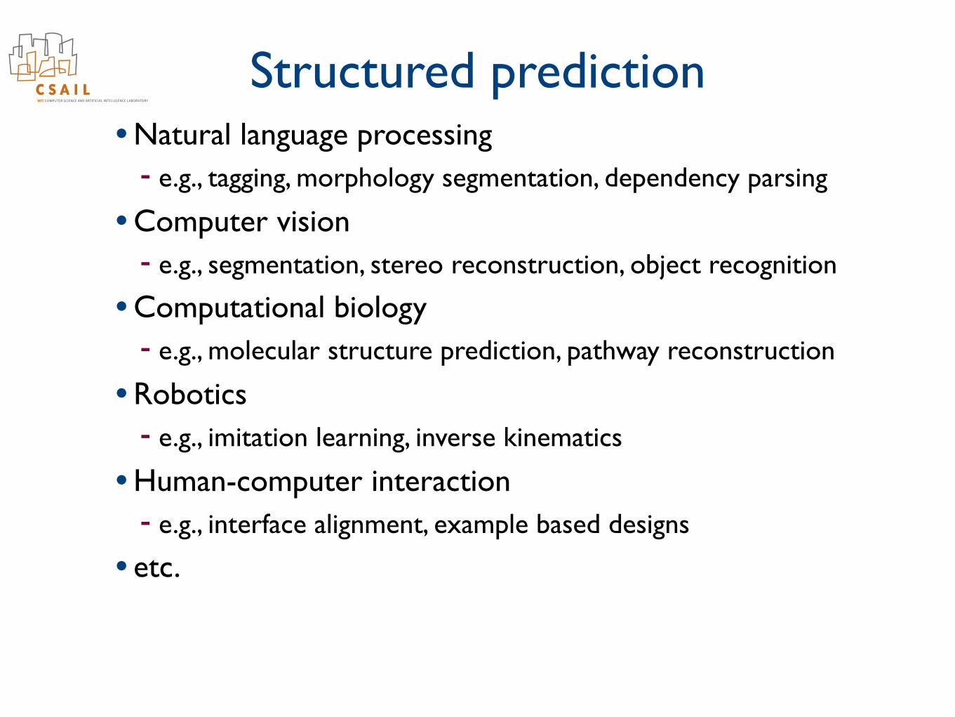
Structured prediction• Natural language processing
- e.g., tagging, morphology segmentation, dependency parsing
• Computer vision- e.g., segmentation, stereo reconstruction, object recognition
• Computational biology- e.g., molecular structure prediction, pathway reconstruction
• Robotics- e.g., imitation learning, inverse kinematics
• Human-computer interaction- e.g., interface alignment, example based designs
• etc.
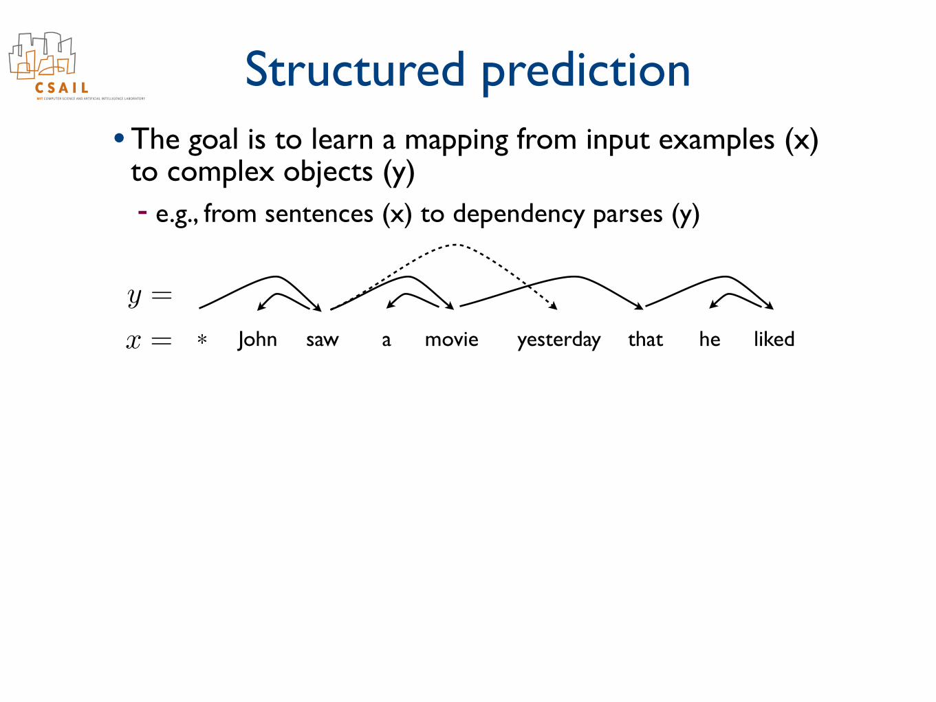
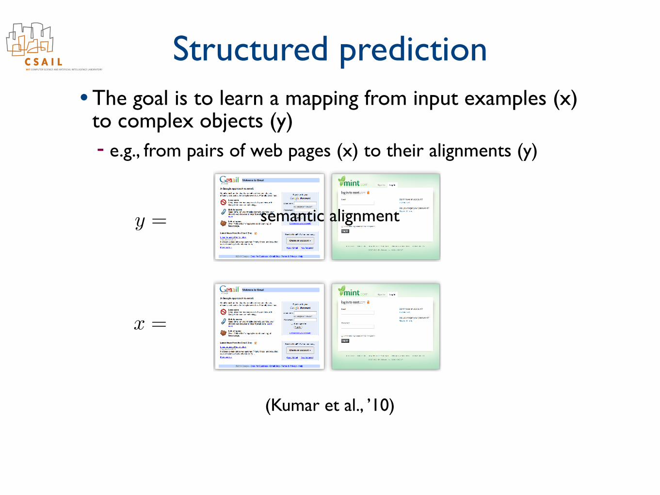
Structured prediction• The goal is to learn a mapping from input examples (x)
to complex objects (y) - e.g., from sentences (x) to dependency parses (y)
John saw a movie yesterday that he liked*x =
y =
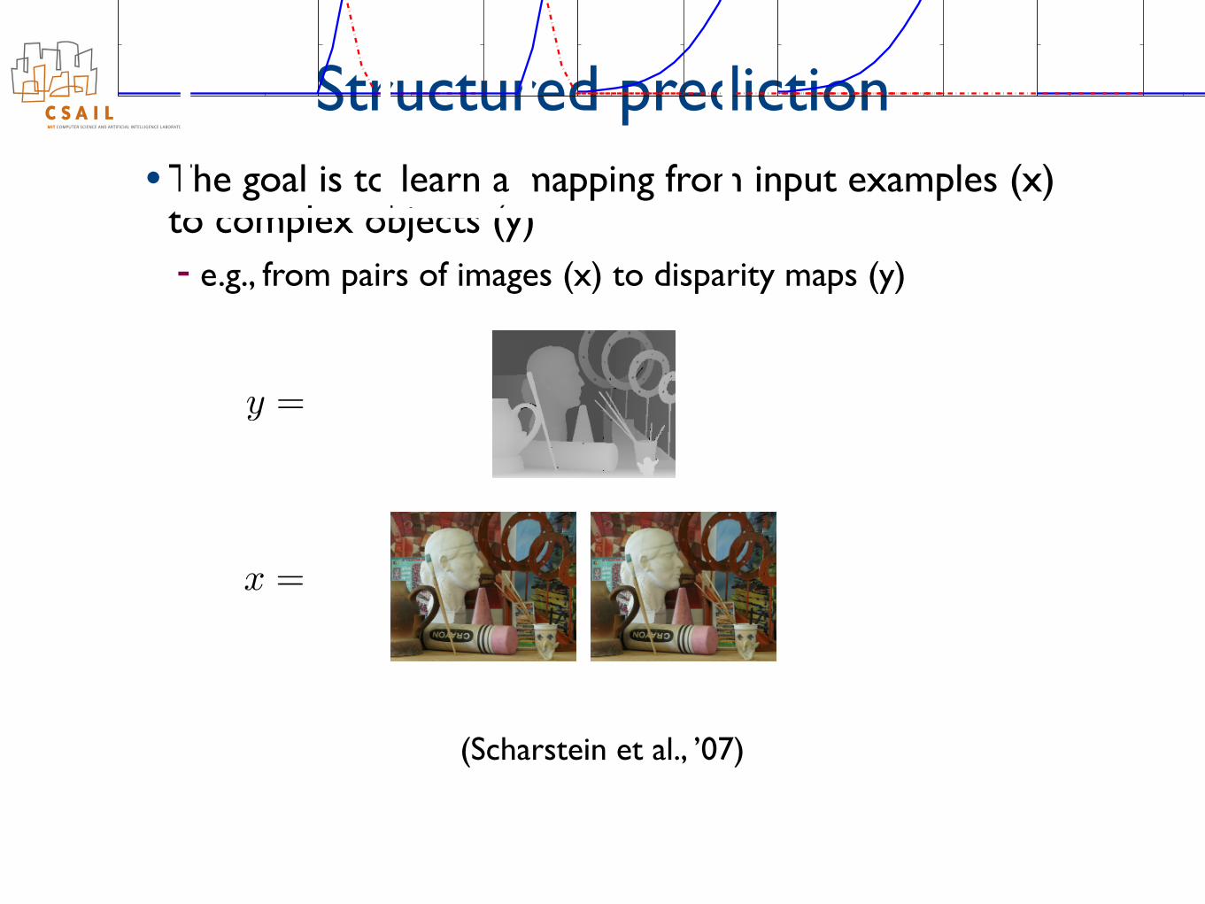
Structured prediction• The goal is to learn a mapping from input examples (x)
to complex objects (y) - e.g., from pairs of images (x) to disparity maps (y)
x =
y =
Small scale validation cont’d• We can also directly examine changes due to OR1 knock-out
Preliminary validation• The �-phage (bacteria infecting virus)!"#$%&'#($)*#+,-./
0#,12(#'
3-142(#
5&1-6#
7&8.6,
OR3 OR1OR2cI cro
cI RNAp2
Arkin et al. 1998
• We can find the equilibrium of the game (binding frequencies)as a function of overall protein concentrations.
50
10!2
100
102
0
0.2
0.4
0.6
0.8
1
Binding in OR
3
frepressor
/fRNA
Bin
din
g F
req
ue
ncy (
tim
e!
ave
rag
e)
RepressorRNA!polymerase
(a) OR3
10!2
100
102
0
0.2
0.4
0.6
0.8
1
Binding in OR
2
frepressor
/fRNA
Bin
din
g F
req
ue
ncy (
tim
e!
ave
rag
e)
RepressorRNA!polymerase
(b) OR2
10!2
100
102
0
0.2
0.4
0.6
0.8
1
Binding in OR
1
frepressor
/fRNA
Bin
din
g F
req
ue
ncy (
tim
e!
ave
rag
e)
RepressorRNA!polymerase
(c) OR1
Figure 3: Predicted protein binding to sites OR3, OR2, and mutated OR1 for increasing amounts of cI2.
became su⇥ciently high do we find cI2 at the mutatedOR1 as well. Note, however, that cI2 inhibits transcrip-tion at OR3 prior to occupying OR1. Thus the bindingat the mutated OR1 could not be observed without in-terventions.
7 Discussion
We believe the game theoretic approach provides a com-pelling causal abstraction of biological systems with re-source constraints. The model is complete with prov-ably convergent algorithms for finding equilibria on agenome-wide scale.
The results from the small scale application are en-couraging. Our model successfully reproduces knownbehavior of the ��switch on the basis of molecularlevel competition and resource constraints, without theneed to assume protein-protein interactions between cI2dimers and cI2 and RNA-polymerase. Even in the con-text of this well-known sub-system, however, few quan-titative experimental results are available about bind-ing. Proper validation and use of our model thereforerelies on estimating the game parameters from availableprotein-DNA binding data (in progress). Once the gameparameters are known, the model provides valid pre-dictions for a number of possible perturbations to thesystem, including changing nuclear concentrations andknock-outs.
Acknowledgments
This work was supported in part by NIH grant GM68762and by NSF ITR grant 0428715. Luis Perez-Breva is a“Fundacion Rafael del Pino” Fellow.
References
[1] Adam Arkin, John Ross, and Harley H. McAdams.Stochastic kinetic analysis of developmental path-way bifurcation in phage �-infected excherichia colicells. Genetics, 149:1633–1648, August 1998.
[2] Kenneth J. Arrow and Gerard Debreu. Existence ofan equilibrium for a competitive economy. Econo-metrica, 22(3):265–290, July 1954.
[3] Z. Bar-Joseph, G. Gerber, T. Lee, N. Rinaldi,J. Yoo, B. Gordon F. Robert, E. Fraenkel,T. Jaakkola, R. Young, and D. Gi�ord. Compu-tational discovery of gene modules and regulatorynetworks. Nature Biotechnology, 21(11):1337–1342,2003.
[4] Otto G. Berg, Robert B. Winter, and Peter H. vonHippel. Di�usion- driven mechanisms of proteintranslocation on nucleic acids. 1. models and theory.Biochemistry, 20(24):6929–48, November 1981.
[5] Drew Fudenberg and Jean Tirole. Game Theory.The MIT Press, 1991.
10
• Predictions are again qualitatively correct
52
Structured Prediction• Prediction is often done by maximizing an MRF
x
s(y;x) =X
f
✓f (yf ;x)
max
ys(y;x)
y
• We’d like to learn these functions from data.
Art Books Dolls Laundry Moebius ReindeerFigure 2. The six datasets used in this paper. Shown is the left image of each pair and the corresponding ground-truth disparities.
have an MPE estimate from running graph cuts we use itto compute our expectation in a manner similar to the em-pirical distribution. Training a lattice-structured model us-ing the approach described here is thus a generalization ofViterbi path-based methods described in [32]. For our learn-ing experiments we use straightforward gradient-based up-dates with a variable learning rate.
4. Datasets
In order to obtain a significant amount of training datafor stereo learning approaches, we have created 30 newstereo datasets with ground-truth disparities using an auto-mated version of the structured-lighting technique of [2].Our datasets are available for use by other researchersat http://vision.middlebury.edu/stereo/data/.Each dataset consists of 7 rectified views taken fromequidistant points along a line, as well as ground-truth dis-parity maps for viewpoints 2 and 6. The images are about1300 ⇥ 1100 pixels (cropped to the overlapping field ofview), with about 150 different integer disparities present.Each set of 7 views was taken with three different exposuresand under three different lighting conditions, for a total of 9different images from each viewpoint.
For the work reported in this paper we only use the sixdatasets shown in Figure 2: Art, Books, Dolls, Laundry,Moebius and Reindeer. As input images we use a single im-age pair (views 2 and 6) taken with the same exposure andlighting. In future work we plan to ultilize the other viewsand the additional datasets for learning from much largertraining sets. To make the images tractable by the graph-cutstereo matcher, we downsample the original images to onethird of their size, resulting in images of roughly 460⇥ 370
pixels with a disparity range of 80 pixels. The resulting im-ages are still more challenging than standard stereo bench-marks such as the Middlebury Teddy and Cones images,due to their larger disparity range and higher percentage ofuntextured surfaces.
Figure 3. Disparity maps of the entire training set for K = 3 pa-rameters after 0, 10, and 20 iterations. Occluded areas are masked.
5. Experiments
In this section we first examine the convergence of learn-ing for models with different numbers of parameters ✓v , us-ing all six datasets as training set. We then use a leave-one-out approach to evaluate the performance of the learned pa-rameters on a new dataset. Finally, we examine how the
x
y
[Scharstein & Pal 07, Middlebury dataset]
Parameters learned from data
s(y;x,w)
(Scharstein et al., ’07)
Structured prediction• The goal is to learn a mapping from input examples (x)
to complex objects (y) - e.g., from pairs of web pages (x) to their alignments (y)
x =
y =Bricolage: A Structured-Prediction Algorithm for Example-Based Web Design
Ranjitha Kumar Jerry O. Talton Salman Ahmad Scott R KlemmerStanford University⇤
Abstract
The Web today provides a corpus of design examples unparalleledin human history. However, leveraging existing designs to pro-duce new pages is currently difficult. This paper introduces theBricolage algorithm for automatically transferring design and con-tent between Web pages. Bricolage introduces a novel structured-prediction technique that learns to create coherent mappings be-tween pages by training on human-generated exemplars. The pro-duced mappings can then be used to automatically transfer the con-tent from one page into the style and layout of another. We showthat Bricolage can learn to accurately reproduce human page map-pings, and that it provides a general, efficient, and automatic tech-nique for retargeting content between a variety of real Web pages.
1 INTRODUCTIONDesigners in many fields rely on examples for inspiration [Herringet al. 2009], and examples can facilitate better design work [Leeet al. 2010]. Examples can illustrate the space of possible solutions,and also how to implement those possibilities [Brandt et al. 2009;Buxton 2007]. Furthermore, repurposing successful elements fromprior ideas can be more efficient than reinventing them from scratch[Gentner et al. 2001; Kolodner and Wills 1993; Hartmann et al.2007].
The Web today provides a corpus of design examples unparalleledin human history. Unfortunately, this powerful resource is un-derutilized. While current systems assist with browsing examples[Lee et al. 2010] and cloning individual design elements [Fitzger-ald 2008], adapting the gestalt structure of Web designs remains atime-intensive, manual process.
Most design reuse today is accomplished via templates, which arespecially created for this purpose [Gibson et al. 2005]. With tem-plates’ standardized page semantics, people can render content intopredesigned layouts. This strength is also a weakness: templateshomogenize page structure, limit customization and creativity, andyield cookie-cutter designs. Ideally, tools should offer both the easeof templates and the diversity of the entire Web. What if any Webpage could be a design template?
This paper introduces the Bricolage algorithm for automaticallytransferring design and content between Web pages. Bricolagematches visually and semantically similar elements in pages to cre-ate coherent mappings between them. These mappings can then beused to transfer the content from one page into the style and layoutof the other, without any user intervention (Figure 1).
Bricolage learns how to transfer content between pages by train-ing on a corpus of exemplar mappings. To generate this corpus, wecreated a Web-based crowdsourcing interface for collecting human-generated mappings. The collector was populated with 50 popularWeb pages, and 39 participants with some Web design experiencewere recruited to specify correspondences between two to four pairsof pages each. After matching every fifth element, participants alsoanswered a free-response question about their rationale. The result-ing data was used to guide the development of the algorithm, trainBricolage’s machine learning components, and verify the results.
⇤e-mail:{ranju,jtalton,saahmad,srk}@cs.stanford.eduUNPUBLISHED TECHNICAL REPORT
Figure 1: Bricolage computes coherent mappings between Webpages by matching visually and semantically similar page elements.The produced mapping can then be used to guide the transfer ofcontent from one page into the design and layout of the other.
Since the mappings collected in our study are highly structured andhierarchical, Bricolage employs structured prediction techniques tomake the mapping process tractable. Each page is segmented intoa tree of contiguous regions, and mappings are predicted betweenpages by identifying elements in these trees. Bricolage introducesa novel tree matching algorithm that allows local and global con-straints to be optimized simultaneously. The algorithm matchessimilar elements between pages while preserving important struc-tural relationships across the trees.
This paper presents the page segmentation algorithm, the data col-lection study, the mapping algorithm, and the machine learningmethod. It then shows results demonstrating that Bricolage canlearn to reproduce human mappings with a high degree of accu-racy. Lastly, it gives examples of Bricolage being used for creat-ing design alternatives, including rapid prototyping and retargetingcontent to alternate form factors such as mobile devices.
2 PAGE SEGMENTATION
Creating mappings between Web pages is facilitated by hav-ing some abstract representation of each page’s structure that isamenable to matching. One candidate for this representation is theDocument Object Model tree of the page, which provides a directcorrespondence between each page region and the HTML that com-prises it. However, the DOM may contain many nodes that have novisual effect on the rendered page, and lack other high-level struc-tures that human viewers might expect.
semantic alignment
(Kumar et al., ’10)
Structured prediction• Natural language processing
- e.g., tagging, morphology segmentation, dependency parsing
• Computer vision- e.g., segmentation, stereo reconstruction, object recognition
• Computational biology- e.g., molecular structure prediction, pathway reconstruction
• Robotics- e.g., imitation learning, inverse kinematics
• Human-computer interaction- e.g., interface alignment, example based designs
• etc.
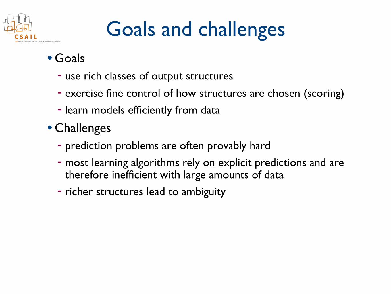
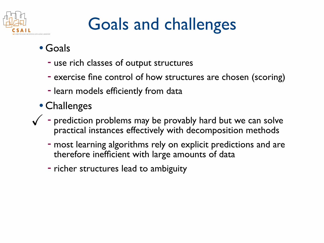
Goals and challenges• Goals
- use rich classes of output structures- exercise fine control of how structures are chosen (scoring)- learn models efficiently from data
• Challenges- prediction problems are often provably hard- most learning algorithms rely on explicit predictions and are
therefore inefficient with large amounts of data- richer structures lead to ambiguity
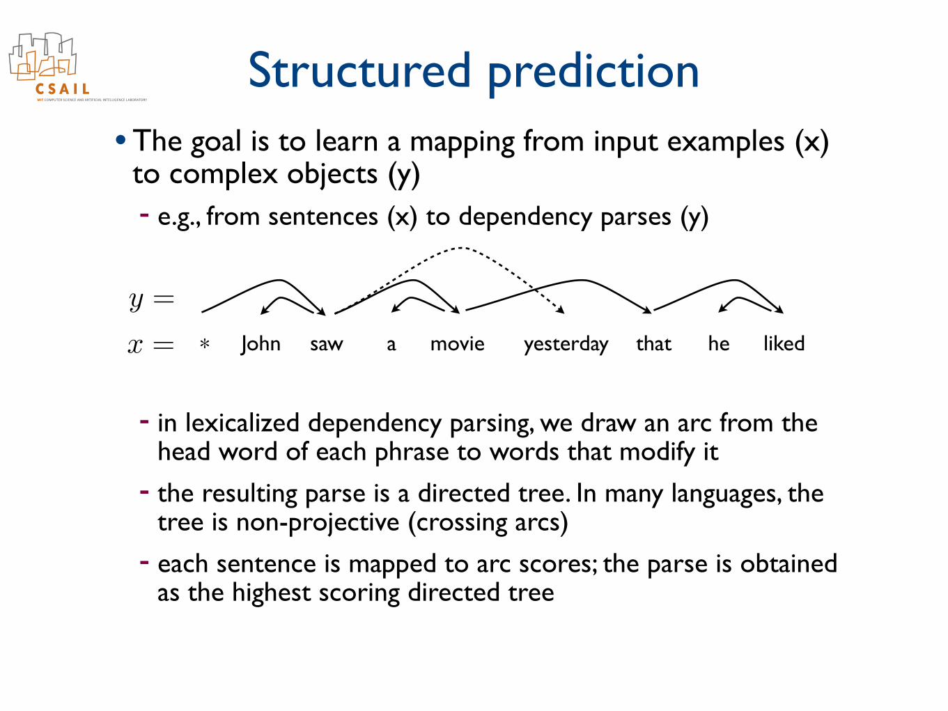
Structured prediction• The goal is to learn a mapping from input examples (x)
to complex objects (y) - e.g., from sentences (x) to dependency parses (y)
- in lexicalized dependency parsing, we draw an arc from the head word of each phrase to words that modify it
- the resulting parse is a directed tree. In many languages, the tree is non-projective (crossing arcs)
- each sentence is mapped to arc scores; the parse is obtained as the highest scoring directed tree
John saw a movie yesterday that he liked*x =
y =
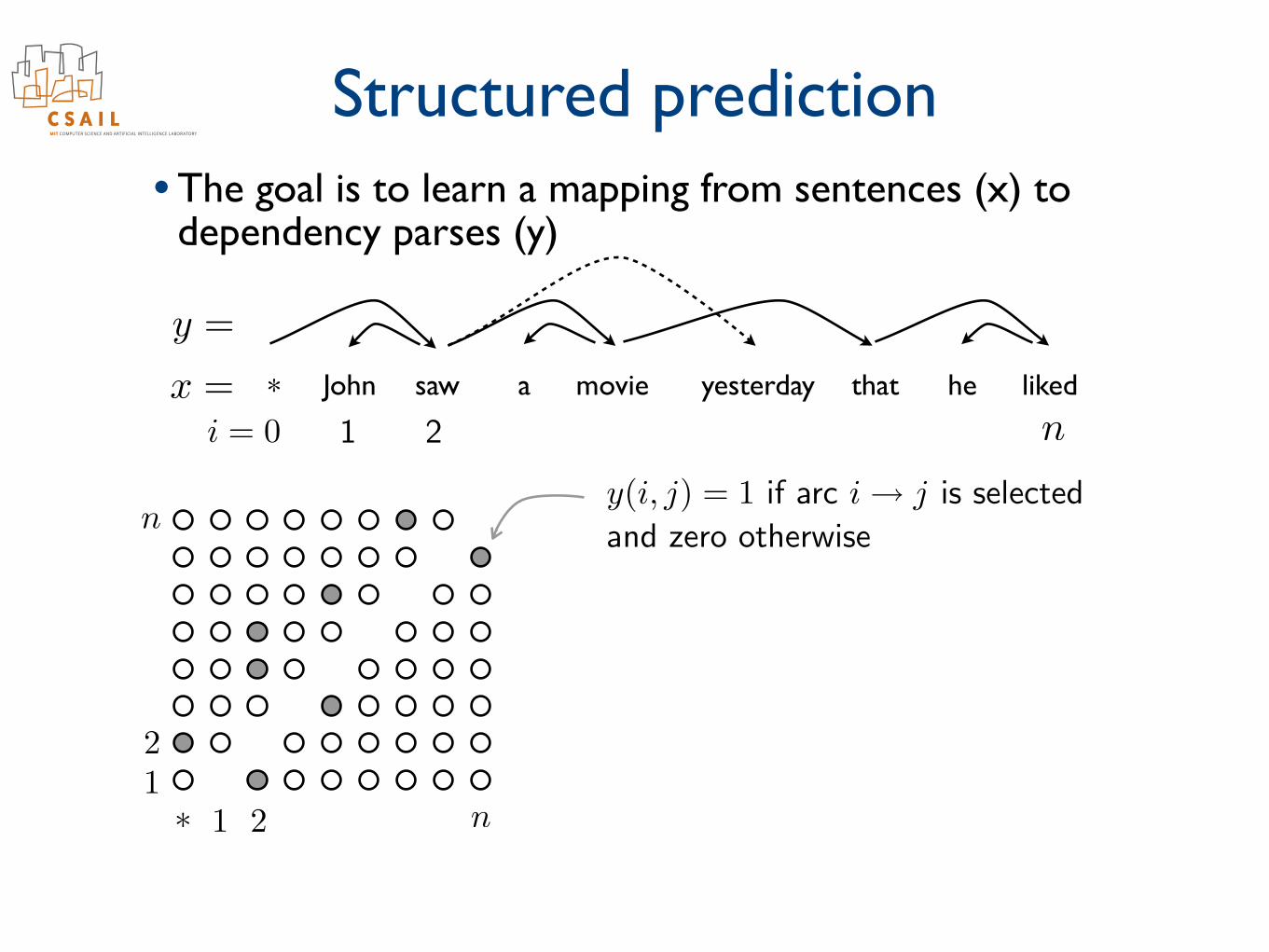
Structured prediction• The goal is to learn a mapping from sentences (x) to
dependency parses (y)
John saw a movie yesterday that he liked*x =
y =
ni = 0 1 2
⇤ 1 2 n12
ny(i, j) = 1 if arc i! j is selected
and zero otherwise
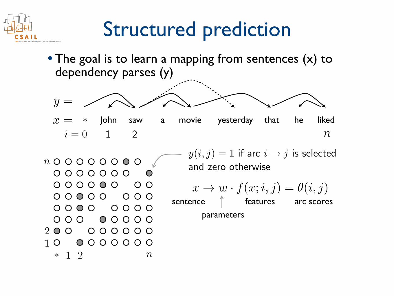
Structured prediction• The goal is to learn a mapping from sentences (x) to
dependency parses (y)
John saw a movie yesterday that he liked*x =
y =
ni = 0 1 2
⇤ 1 2 n12
ny(i, j) = 1 if arc i! j is selected
and zero otherwise
x ! w · f(x; i, j) = ✓(i, j)
parametersfeatures arc scoressentence
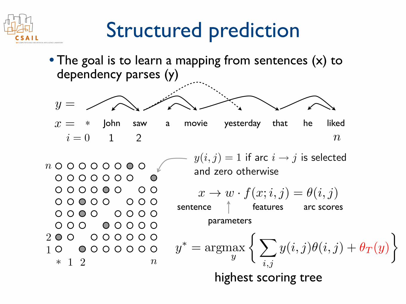
Structured prediction• The goal is to learn a mapping from sentences (x) to
dependency parses (y)
John saw a movie yesterday that he liked*x =
y =
ni = 0 1 2
⇤ 1 2 n12
ny(i, j) = 1 if arc i! j is selected
and zero otherwise
x ! w · f(x; i, j) = ✓(i, j)
parametersfeatures arc scoressentence
y⇤ = argmax
y
⇢X
i,j
y(i, j)✓(i, j) + ✓T (y)
�
highest scoring tree
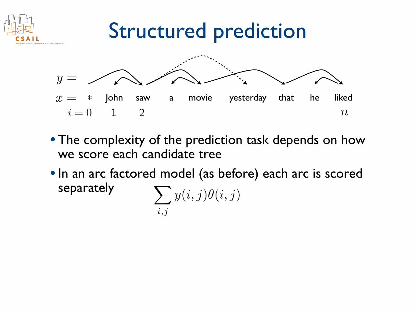
Structured prediction
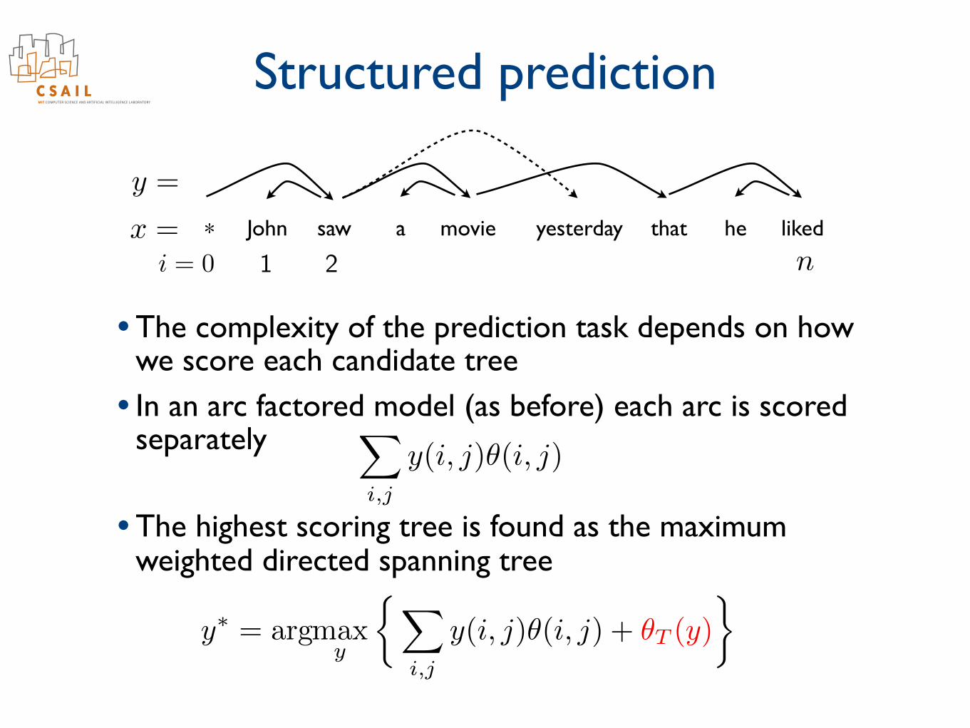
• The complexity of the prediction task depends on how we score each candidate tree
• In an arc factored model (as before) each arc is scored separately
• The highest scoring tree is found as the maximum weighted directed spanning tree
John saw a movie yesterday that he liked*x =
y =
ni = 0 1 2
y⇤ = argmax
y
⇢X
i,j
y(i, j)✓(i, j) + ✓T (y)
�
X
i,j
y(i, j)✓(i, j)
Structured prediction
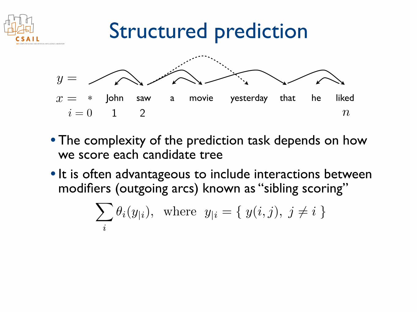
• The complexity of the prediction task depends on how we score each candidate tree
• It is often advantageous to include interactions between modifiers (outgoing arcs) known as “sibling scoring”
John saw a movie yesterday that he liked*x =
y =
ni = 0 1 2
X
i
✓i(y|i), where y|i = { y(i, j), j 6= i }
Structured prediction
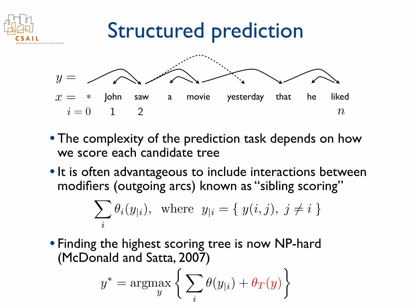
• The complexity of the prediction task depends on how we score each candidate tree
• It is often advantageous to include interactions between modifiers (outgoing arcs) known as “sibling scoring”
• Finding the highest scoring tree is now NP-hard (McDonald and Satta, 2007)
John saw a movie yesterday that he liked*x =
y =
ni = 0 1 2
X
i
✓i(y|i), where y|i = { y(i, j), j 6= i }
y⇤ = argmax
y
⇢X
i
✓(y|i) + ✓T (y)
�
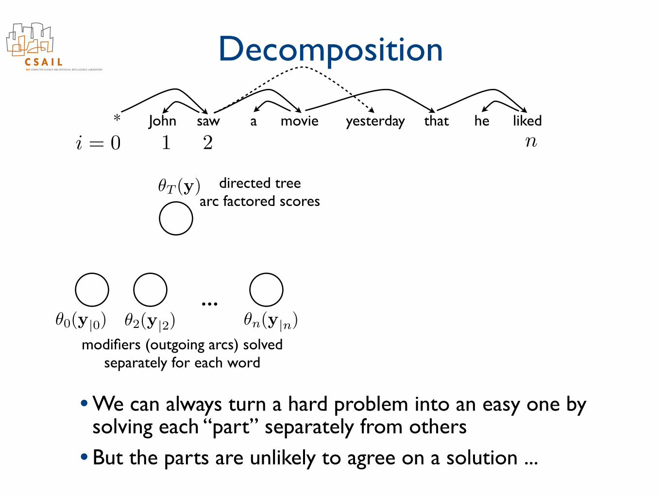
Decomposition
...
i = 0 1 2 n* John saw a movie yesterday that he liked
✓0(y|0) ✓2(y|2) ✓n(y|n)
✓T (y) directed treearc factored scores
modifiers (outgoing arcs) solvedseparately for each word
• We can always turn a hard problem into an easy one by solving each “part” separately from others
• But the parts are unlikely to agree on a solution ...
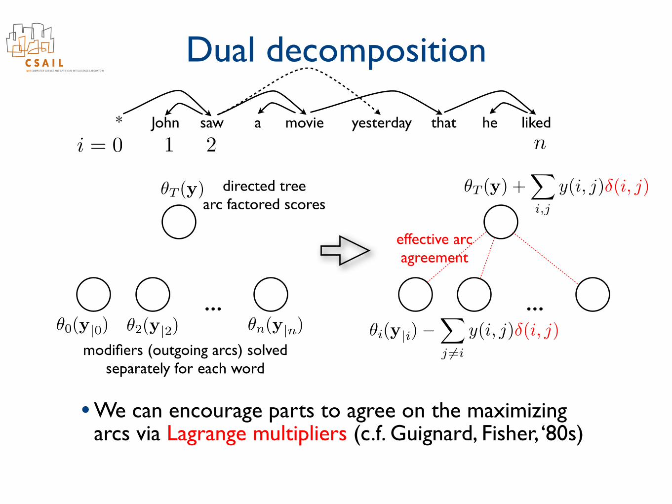
Dual decomposition
...
i = 0 1 2 n* John saw a movie yesterday that he liked
✓0(y|0) ✓2(y|2) ✓n(y|n)
✓T (y) directed treearc factored scores
modifiers (outgoing arcs) solvedseparately for each word
• We can encourage parts to agree on the maximizing arcs via Lagrange multipliers (c.f. Guignard, Fisher, ‘80s)
...
✓T (y) +X
i,j
y(i, j)�(i, j)
✓i(y|i)�X
j 6=i
y(i, j)�(i, j)
effective arc agreement
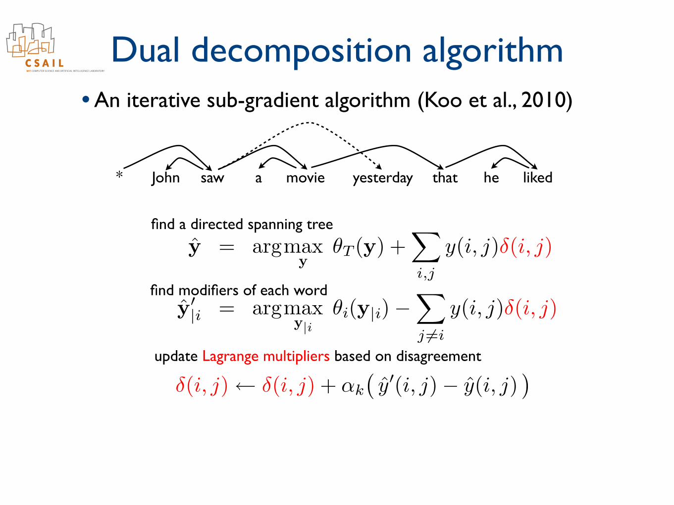
Dual decomposition algorithm• An iterative sub-gradient algorithm (Koo et al., 2010)
find a directed spanning tree
find modifiers of each word
update Lagrange multipliers based on disagreement
�(i, j) �(i, j) + ↵k
�y0(i, j)� y(i, j)
�
* John saw a movie yesterday that he liked
ˆy = argmax
y✓T (y) +
X
i,j
y(i, j)�(i, j)
ˆy0|i = argmax
y|i✓i(y|i)�
X
j 6=i
y(i, j)�(i, j)
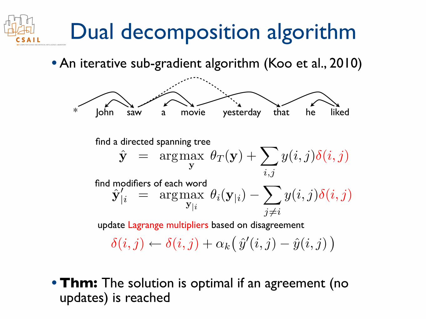
Dual decomposition algorithm• An iterative sub-gradient algorithm (Koo et al., 2010)
• Thm: The solution is optimal if an agreement (no updates) is reached
find a directed spanning tree
find modifiers of each word
update Lagrange multipliers based on disagreement
�(i, j) �(i, j) + ↵k
�y0(i, j)� y(i, j)
�
* John saw a movie yesterday that he liked
ˆy = argmax
y✓T (y) +
X
i,j
y(i, j)�(i, j)
ˆy0|i = argmax
y|i✓i(y|i)�
X
j 6=i
y(i, j)�(i, j)
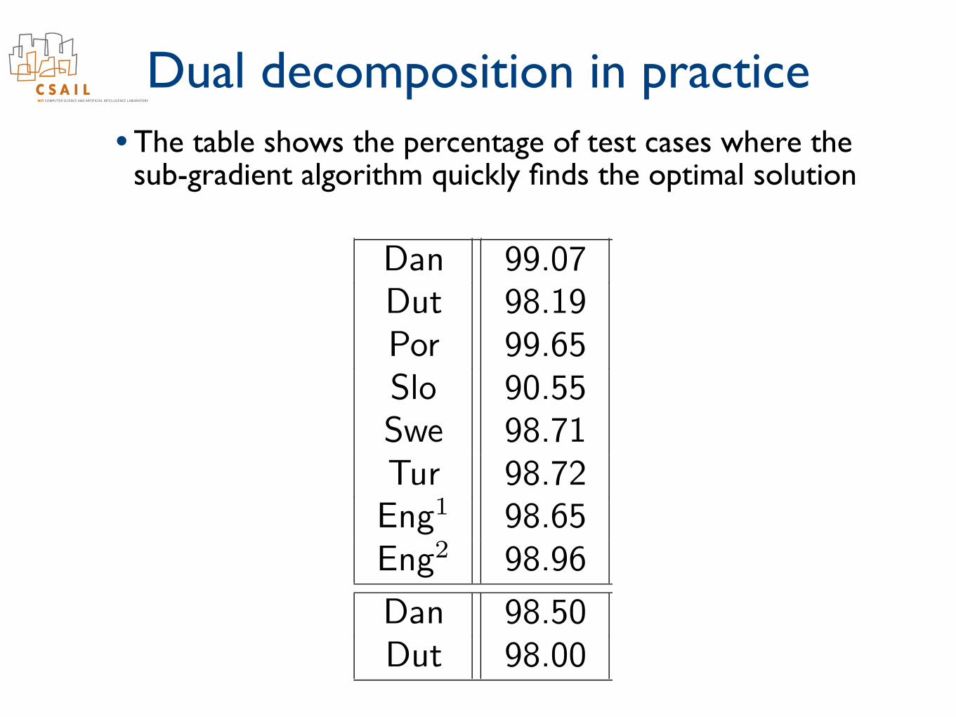
Convergence
CertS CertGDan 99.07 98.45Dut 98.19 97.93Por 99.65 99.31Slo 90.55 95.27Swe 98.71 98.97Tur 98.72 99.04Eng1 98.65 99.18Eng2 98.96 99.12
Dan 98.50 98.50Dut 98.00 99.50
CertS CertGPTB 98.89 98.63PDT 96.67 96.43
(Percentage of test data sentences where a certificate of optimalityis provided, with K = 5000)
• The table shows the percentage of test cases where the sub-gradient algorithm quickly finds the optimal solution
Dual decomposition in practice
Goals and challenges• Goals
- use rich classes of output structures- exercise fine control of how structures are chosen (scoring)- learn models efficiently from data
• Challenges- prediction problems may be provably hard but we can solve
practical instances effectively with decomposition methods- most learning algorithms rely on explicit predictions and are
therefore inefficient with large amounts of data- richer structures lead to ambiguity
X
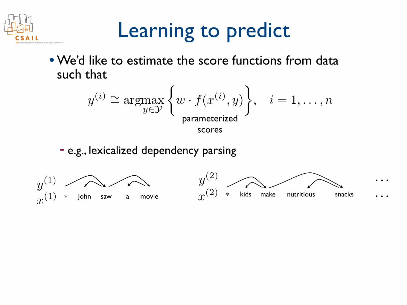
Learning to predict• We’d like to estimate the score functions from data
such that
- e.g., lexicalized dependency parsing
. . .
parameterizedscores
y
(i) ⇠=
argmax
y2Y
⇢w · f(x(i)
, y)
�, i = 1, . . . , n
John saw a movie* kids make nutritious snacks*x
(1)y(1)
x
(2)y(2) . . .
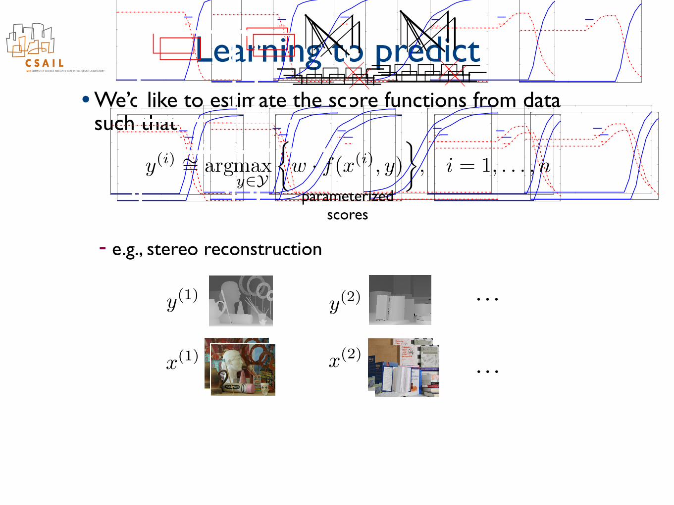
Learning to predict• We’d like to estimate the score functions from data
such that
- e.g., stereo reconstruction
Small scale validation cont’d• We can also directly examine changes due to OR1 knock-out
Preliminary validation• The �-phage (bacteria infecting virus)!"#$%&'#($)*#+,-./
0#,12(#'
3-142(#
5&1-6#
7&8.6,
OR3 OR1OR2cI cro
cI RNAp2
Arkin et al. 1998
• We can find the equilibrium of the game (binding frequencies)as a function of overall protein concentrations.
50
10!2
100
102
0
0.2
0.4
0.6
0.8
1
Binding in OR
3
frepressor
/fRNA
Bin
din
g F
req
ue
ncy (
tim
e!
ave
rag
e)
RepressorRNA!polymerase
(a) OR3
10!2
100
102
0
0.2
0.4
0.6
0.8
1
Binding in OR
2
frepressor
/fRNA
Bin
din
g F
req
ue
ncy (
tim
e!
ave
rag
e)
RepressorRNA!polymerase
(b) OR2
10!2
100
102
0
0.2
0.4
0.6
0.8
1
Binding in OR
1
frepressor
/fRNA
Bin
din
g F
req
ue
ncy (
tim
e!
ave
rag
e)
RepressorRNA!polymerase
(c) OR1
Figure 3: Predicted protein binding to sites OR3, OR2, and mutated OR1 for increasing amounts of cI2.
became su⇥ciently high do we find cI2 at the mutatedOR1 as well. Note, however, that cI2 inhibits transcrip-tion at OR3 prior to occupying OR1. Thus the bindingat the mutated OR1 could not be observed without in-terventions.
7 Discussion
We believe the game theoretic approach provides a com-pelling causal abstraction of biological systems with re-source constraints. The model is complete with prov-ably convergent algorithms for finding equilibria on agenome-wide scale.
The results from the small scale application are en-couraging. Our model successfully reproduces knownbehavior of the ��switch on the basis of molecularlevel competition and resource constraints, without theneed to assume protein-protein interactions between cI2dimers and cI2 and RNA-polymerase. Even in the con-text of this well-known sub-system, however, few quan-titative experimental results are available about bind-ing. Proper validation and use of our model thereforerelies on estimating the game parameters from availableprotein-DNA binding data (in progress). Once the gameparameters are known, the model provides valid pre-dictions for a number of possible perturbations to thesystem, including changing nuclear concentrations andknock-outs.
Acknowledgments
This work was supported in part by NIH grant GM68762and by NSF ITR grant 0428715. Luis Perez-Breva is a“Fundacion Rafael del Pino” Fellow.
References
[1] Adam Arkin, John Ross, and Harley H. McAdams.Stochastic kinetic analysis of developmental path-way bifurcation in phage �-infected excherichia colicells. Genetics, 149:1633–1648, August 1998.
[2] Kenneth J. Arrow and Gerard Debreu. Existence ofan equilibrium for a competitive economy. Econo-metrica, 22(3):265–290, July 1954.
[3] Z. Bar-Joseph, G. Gerber, T. Lee, N. Rinaldi,J. Yoo, B. Gordon F. Robert, E. Fraenkel,T. Jaakkola, R. Young, and D. Gi�ord. Compu-tational discovery of gene modules and regulatorynetworks. Nature Biotechnology, 21(11):1337–1342,2003.
[4] Otto G. Berg, Robert B. Winter, and Peter H. vonHippel. Di�usion- driven mechanisms of proteintranslocation on nucleic acids. 1. models and theory.Biochemistry, 20(24):6929–48, November 1981.
[5] Drew Fudenberg and Jean Tirole. Game Theory.The MIT Press, 1991.
10
• Predictions are again qualitatively correct
52
Structured Prediction• Prediction is often done by maximizing an MRF
x
s(y;x) =X
f
✓f (yf ;x)
max
ys(y;x)
y
• We’d like to learn these functions from data.
Art Books Dolls Laundry Moebius ReindeerFigure 2. The six datasets used in this paper. Shown is the left image of each pair and the corresponding ground-truth disparities.
have an MPE estimate from running graph cuts we use itto compute our expectation in a manner similar to the em-pirical distribution. Training a lattice-structured model us-ing the approach described here is thus a generalization ofViterbi path-based methods described in [32]. For our learn-ing experiments we use straightforward gradient-based up-dates with a variable learning rate.
4. Datasets
In order to obtain a significant amount of training datafor stereo learning approaches, we have created 30 newstereo datasets with ground-truth disparities using an auto-mated version of the structured-lighting technique of [2].Our datasets are available for use by other researchersat http://vision.middlebury.edu/stereo/data/.Each dataset consists of 7 rectified views taken fromequidistant points along a line, as well as ground-truth dis-parity maps for viewpoints 2 and 6. The images are about1300 ⇥ 1100 pixels (cropped to the overlapping field ofview), with about 150 different integer disparities present.Each set of 7 views was taken with three different exposuresand under three different lighting conditions, for a total of 9different images from each viewpoint.
For the work reported in this paper we only use the sixdatasets shown in Figure 2: Art, Books, Dolls, Laundry,Moebius and Reindeer. As input images we use a single im-age pair (views 2 and 6) taken with the same exposure andlighting. In future work we plan to ultilize the other viewsand the additional datasets for learning from much largertraining sets. To make the images tractable by the graph-cutstereo matcher, we downsample the original images to onethird of their size, resulting in images of roughly 460⇥ 370
pixels with a disparity range of 80 pixels. The resulting im-ages are still more challenging than standard stereo bench-marks such as the Middlebury Teddy and Cones images,due to their larger disparity range and higher percentage ofuntextured surfaces.
Figure 3. Disparity maps of the entire training set for K = 3 pa-rameters after 0, 10, and 20 iterations. Occluded areas are masked.
5. Experiments
In this section we first examine the convergence of learn-ing for models with different numbers of parameters ✓v , us-ing all six datasets as training set. We then use a leave-one-out approach to evaluate the performance of the learned pa-rameters on a new dataset. Finally, we examine how the
x
y
[Scharstein & Pal 07, Middlebury dataset]
Parameters learned from data
s(y;x,w)
Small scale validation cont’d• We can also directly examine changes due to OR1 knock-out
Preliminary validation• The �-phage (bacteria infecting virus)!"#$%&'#($)*#+,-./
0#,12(#'
3-142(#
5&1-6#
7&8.6,
OR3 OR1OR2cI cro
cI RNAp2
Arkin et al. 1998
• We can find the equilibrium of the game (binding frequencies)as a function of overall protein concentrations.
50
10!2
100
102
0
0.2
0.4
0.6
0.8
1
Binding in OR
3
frepressor
/fRNA
Bin
din
g F
requency (
tim
e!
avera
ge)
RepressorRNA!polymerase
(a) OR3
10!2
100
102
0
0.2
0.4
0.6
0.8
1
Binding in OR
2
frepressor
/fRNA
Bin
din
g F
requency (
tim
e!
avera
ge)
RepressorRNA!polymerase
(b) OR2
10!2
100
102
0
0.2
0.4
0.6
0.8
1
Binding in OR
1
frepressor
/fRNA
Bin
din
g F
requency (
tim
e!
avera
ge)
RepressorRNA!polymerase
(c) OR1
Figure 3: Predicted protein binding to sites OR3, OR2, and mutated OR1 for increasing amounts of cI2.
became su⇥ciently high do we find cI2 at the mutatedOR1 as well. Note, however, that cI2 inhibits transcrip-tion at OR3 prior to occupying OR1. Thus the bindingat the mutated OR1 could not be observed without in-terventions.
7 Discussion
We believe the game theoretic approach provides a com-pelling causal abstraction of biological systems with re-source constraints. The model is complete with prov-ably convergent algorithms for finding equilibria on agenome-wide scale.
The results from the small scale application are en-couraging. Our model successfully reproduces knownbehavior of the ��switch on the basis of molecularlevel competition and resource constraints, without theneed to assume protein-protein interactions between cI2dimers and cI2 and RNA-polymerase. Even in the con-text of this well-known sub-system, however, few quan-titative experimental results are available about bind-ing. Proper validation and use of our model thereforerelies on estimating the game parameters from availableprotein-DNA binding data (in progress). Once the gameparameters are known, the model provides valid pre-dictions for a number of possible perturbations to thesystem, including changing nuclear concentrations andknock-outs.
Acknowledgments
This work was supported in part by NIH grant GM68762and by NSF ITR grant 0428715. Luis Perez-Breva is a“Fundacion Rafael del Pino” Fellow.
References
[1] Adam Arkin, John Ross, and Harley H. McAdams.Stochastic kinetic analysis of developmental path-way bifurcation in phage �-infected excherichia colicells. Genetics, 149:1633–1648, August 1998.
[2] Kenneth J. Arrow and Gerard Debreu. Existence ofan equilibrium for a competitive economy. Econo-metrica, 22(3):265–290, July 1954.
[3] Z. Bar-Joseph, G. Gerber, T. Lee, N. Rinaldi,J. Yoo, B. Gordon F. Robert, E. Fraenkel,T. Jaakkola, R. Young, and D. Gi�ord. Compu-tational discovery of gene modules and regulatorynetworks. Nature Biotechnology, 21(11):1337–1342,2003.
[4] Otto G. Berg, Robert B. Winter, and Peter H. vonHippel. Di�usion- driven mechanisms of proteintranslocation on nucleic acids. 1. models and theory.Biochemistry, 20(24):6929–48, November 1981.
[5] Drew Fudenberg and Jean Tirole. Game Theory.The MIT Press, 1991.
10
• Predictions are again qualitatively correct
52
Structured Prediction• Prediction is often done by maximizing an MRF
x
s(y;x) =X
f
✓f (yf ;x)
max
ys(y;x)
y
• We’d like to learn these functions from data.
Art Books Dolls Laundry Moebius ReindeerFigure 2. The six datasets used in this paper. Shown is the left image of each pair and the corresponding ground-truth disparities.
have an MPE estimate from running graph cuts we use itto compute our expectation in a manner similar to the em-pirical distribution. Training a lattice-structured model us-ing the approach described here is thus a generalization ofViterbi path-based methods described in [32]. For our learn-ing experiments we use straightforward gradient-based up-dates with a variable learning rate.
4. Datasets
In order to obtain a significant amount of training datafor stereo learning approaches, we have created 30 newstereo datasets with ground-truth disparities using an auto-mated version of the structured-lighting technique of [2].Our datasets are available for use by other researchersat http://vision.middlebury.edu/stereo/data/.Each dataset consists of 7 rectified views taken fromequidistant points along a line, as well as ground-truth dis-parity maps for viewpoints 2 and 6. The images are about1300 ⇥ 1100 pixels (cropped to the overlapping field ofview), with about 150 different integer disparities present.Each set of 7 views was taken with three different exposuresand under three different lighting conditions, for a total of 9different images from each viewpoint.
For the work reported in this paper we only use the sixdatasets shown in Figure 2: Art, Books, Dolls, Laundry,Moebius and Reindeer. As input images we use a single im-age pair (views 2 and 6) taken with the same exposure andlighting. In future work we plan to ultilize the other viewsand the additional datasets for learning from much largertraining sets. To make the images tractable by the graph-cutstereo matcher, we downsample the original images to onethird of their size, resulting in images of roughly 460⇥ 370
pixels with a disparity range of 80 pixels. The resulting im-ages are still more challenging than standard stereo bench-marks such as the Middlebury Teddy and Cones images,due to their larger disparity range and higher percentage ofuntextured surfaces.
Figure 3. Disparity maps of the entire training set for K = 3 pa-rameters after 0, 10, and 20 iterations. Occluded areas are masked.
5. Experiments
In this section we first examine the convergence of learn-ing for models with different numbers of parameters ✓v , us-ing all six datasets as training set. We then use a leave-one-out approach to evaluate the performance of the learned pa-rameters on a new dataset. Finally, we examine how the
x
y
[Scharstein & Pal 07, Middlebury dataset]
Parameters learned from data
s(y;x,w)
Small scale validation cont’d• We can also directly examine changes due to OR1 knock-out
Preliminary validation• The �-phage (bacteria infecting virus)!"#$%&'#($)*#+,-./
0#,12(#'
3-142(#
5&1-6#
7&8.6,
OR3 OR1OR2cI cro
cI RNAp2
Arkin et al. 1998
• We can find the equilibrium of the game (binding frequencies)as a function of overall protein concentrations.
50
10!2
100
102
0
0.2
0.4
0.6
0.8
1
Binding in OR
3
frepressor
/fRNA
Bin
din
g F
req
ue
ncy (
tim
e!
ave
rag
e)
RepressorRNA!polymerase
(a) OR3
10!2
100
102
0
0.2
0.4
0.6
0.8
1
Binding in OR
2
frepressor
/fRNA
Bin
din
g F
req
ue
ncy (
tim
e!
ave
rag
e)
RepressorRNA!polymerase
(b) OR2
10!2
100
102
0
0.2
0.4
0.6
0.8
1
Binding in OR
1
frepressor
/fRNA
Bin
din
g F
req
ue
ncy (
tim
e!
ave
rag
e)
RepressorRNA!polymerase
(c) OR1
Figure 3: Predicted protein binding to sites OR3, OR2, and mutated OR1 for increasing amounts of cI2.
became su⇥ciently high do we find cI2 at the mutatedOR1 as well. Note, however, that cI2 inhibits transcrip-tion at OR3 prior to occupying OR1. Thus the bindingat the mutated OR1 could not be observed without in-terventions.
7 Discussion
We believe the game theoretic approach provides a com-pelling causal abstraction of biological systems with re-source constraints. The model is complete with prov-ably convergent algorithms for finding equilibria on agenome-wide scale.
The results from the small scale application are en-couraging. Our model successfully reproduces knownbehavior of the ��switch on the basis of molecularlevel competition and resource constraints, without theneed to assume protein-protein interactions between cI2dimers and cI2 and RNA-polymerase. Even in the con-text of this well-known sub-system, however, few quan-titative experimental results are available about bind-ing. Proper validation and use of our model thereforerelies on estimating the game parameters from availableprotein-DNA binding data (in progress). Once the gameparameters are known, the model provides valid pre-dictions for a number of possible perturbations to thesystem, including changing nuclear concentrations andknock-outs.
Acknowledgments
This work was supported in part by NIH grant GM68762and by NSF ITR grant 0428715. Luis Perez-Breva is a“Fundacion Rafael del Pino” Fellow.
References
[1] Adam Arkin, John Ross, and Harley H. McAdams.Stochastic kinetic analysis of developmental path-way bifurcation in phage �-infected excherichia colicells. Genetics, 149:1633–1648, August 1998.
[2] Kenneth J. Arrow and Gerard Debreu. Existence ofan equilibrium for a competitive economy. Econo-metrica, 22(3):265–290, July 1954.
[3] Z. Bar-Joseph, G. Gerber, T. Lee, N. Rinaldi,J. Yoo, B. Gordon F. Robert, E. Fraenkel,T. Jaakkola, R. Young, and D. Gi�ord. Compu-tational discovery of gene modules and regulatorynetworks. Nature Biotechnology, 21(11):1337–1342,2003.
[4] Otto G. Berg, Robert B. Winter, and Peter H. vonHippel. Di�usion- driven mechanisms of proteintranslocation on nucleic acids. 1. models and theory.Biochemistry, 20(24):6929–48, November 1981.
[5] Drew Fudenberg and Jean Tirole. Game Theory.The MIT Press, 1991.
10
• Predictions are again qualitatively correct
52
Structured Prediction• Prediction is often done by maximizing an MRF
x
s(y;x) =X
f
✓f (yf ;x)
max
ys(y;x)
y
• We’d like to learn these functions from data.
Art Books Dolls Laundry Moebius ReindeerFigure 2. The six datasets used in this paper. Shown is the left image of each pair and the corresponding ground-truth disparities.
have an MPE estimate from running graph cuts we use itto compute our expectation in a manner similar to the em-pirical distribution. Training a lattice-structured model us-ing the approach described here is thus a generalization ofViterbi path-based methods described in [32]. For our learn-ing experiments we use straightforward gradient-based up-dates with a variable learning rate.
4. Datasets
In order to obtain a significant amount of training datafor stereo learning approaches, we have created 30 newstereo datasets with ground-truth disparities using an auto-mated version of the structured-lighting technique of [2].Our datasets are available for use by other researchersat http://vision.middlebury.edu/stereo/data/.Each dataset consists of 7 rectified views taken fromequidistant points along a line, as well as ground-truth dis-parity maps for viewpoints 2 and 6. The images are about1300 ⇥ 1100 pixels (cropped to the overlapping field ofview), with about 150 different integer disparities present.Each set of 7 views was taken with three different exposuresand under three different lighting conditions, for a total of 9different images from each viewpoint.
For the work reported in this paper we only use the sixdatasets shown in Figure 2: Art, Books, Dolls, Laundry,Moebius and Reindeer. As input images we use a single im-age pair (views 2 and 6) taken with the same exposure andlighting. In future work we plan to ultilize the other viewsand the additional datasets for learning from much largertraining sets. To make the images tractable by the graph-cutstereo matcher, we downsample the original images to onethird of their size, resulting in images of roughly 460⇥ 370
pixels with a disparity range of 80 pixels. The resulting im-ages are still more challenging than standard stereo bench-marks such as the Middlebury Teddy and Cones images,due to their larger disparity range and higher percentage ofuntextured surfaces.
Figure 3. Disparity maps of the entire training set for K = 3 pa-rameters after 0, 10, and 20 iterations. Occluded areas are masked.
5. Experiments
In this section we first examine the convergence of learn-ing for models with different numbers of parameters ✓v , us-ing all six datasets as training set. We then use a leave-one-out approach to evaluate the performance of the learned pa-rameters on a new dataset. Finally, we examine how the
x
y
[Scharstein & Pal 07, Middlebury dataset]
Parameters learned from data
s(y;x,w)
Small scale validation cont’d• We can also directly examine changes due to OR1 knock-out
Preliminary validation• The �-phage (bacteria infecting virus)!"#$%&'#($)*#+,-./
0#,12(#'
3-142(#
5&1-6#
7&8.6,
OR3 OR1OR2cI cro
cI RNAp2
Arkin et al. 1998
• We can find the equilibrium of the game (binding frequencies)as a function of overall protein concentrations.
50
10!2
100
102
0
0.2
0.4
0.6
0.8
1
Binding in OR
3
frepressor
/fRNA
Bin
din
g F
requency (
tim
e!
avera
ge)
RepressorRNA!polymerase
(a) OR3
10!2
100
102
0
0.2
0.4
0.6
0.8
1
Binding in OR
2
frepressor
/fRNA
Bin
din
g F
requency (
tim
e!
avera
ge)
RepressorRNA!polymerase
(b) OR2
10!2
100
102
0
0.2
0.4
0.6
0.8
1
Binding in OR
1
frepressor
/fRNA
Bin
din
g F
requency (
tim
e!
avera
ge)
RepressorRNA!polymerase
(c) OR1
Figure 3: Predicted protein binding to sites OR3, OR2, and mutated OR1 for increasing amounts of cI2.
became su⇥ciently high do we find cI2 at the mutatedOR1 as well. Note, however, that cI2 inhibits transcrip-tion at OR3 prior to occupying OR1. Thus the bindingat the mutated OR1 could not be observed without in-terventions.
7 Discussion
We believe the game theoretic approach provides a com-pelling causal abstraction of biological systems with re-source constraints. The model is complete with prov-ably convergent algorithms for finding equilibria on agenome-wide scale.
The results from the small scale application are en-couraging. Our model successfully reproduces knownbehavior of the ��switch on the basis of molecularlevel competition and resource constraints, without theneed to assume protein-protein interactions between cI2dimers and cI2 and RNA-polymerase. Even in the con-text of this well-known sub-system, however, few quan-titative experimental results are available about bind-ing. Proper validation and use of our model thereforerelies on estimating the game parameters from availableprotein-DNA binding data (in progress). Once the gameparameters are known, the model provides valid pre-dictions for a number of possible perturbations to thesystem, including changing nuclear concentrations andknock-outs.
Acknowledgments
This work was supported in part by NIH grant GM68762and by NSF ITR grant 0428715. Luis Perez-Breva is a“Fundacion Rafael del Pino” Fellow.
References
[1] Adam Arkin, John Ross, and Harley H. McAdams.Stochastic kinetic analysis of developmental path-way bifurcation in phage �-infected excherichia colicells. Genetics, 149:1633–1648, August 1998.
[2] Kenneth J. Arrow and Gerard Debreu. Existence ofan equilibrium for a competitive economy. Econo-metrica, 22(3):265–290, July 1954.
[3] Z. Bar-Joseph, G. Gerber, T. Lee, N. Rinaldi,J. Yoo, B. Gordon F. Robert, E. Fraenkel,T. Jaakkola, R. Young, and D. Gi�ord. Compu-tational discovery of gene modules and regulatorynetworks. Nature Biotechnology, 21(11):1337–1342,2003.
[4] Otto G. Berg, Robert B. Winter, and Peter H. vonHippel. Di�usion- driven mechanisms of proteintranslocation on nucleic acids. 1. models and theory.Biochemistry, 20(24):6929–48, November 1981.
[5] Drew Fudenberg and Jean Tirole. Game Theory.The MIT Press, 1991.
10
• Predictions are again qualitatively correct
52
Structured Prediction• Prediction is often done by maximizing an MRF
x
s(y;x) =X
f
✓f (yf ;x)
max
ys(y;x)
y
• We’d like to learn these functions from data.
Art Books Dolls Laundry Moebius ReindeerFigure 2. The six datasets used in this paper. Shown is the left image of each pair and the corresponding ground-truth disparities.
have an MPE estimate from running graph cuts we use itto compute our expectation in a manner similar to the em-pirical distribution. Training a lattice-structured model us-ing the approach described here is thus a generalization ofViterbi path-based methods described in [32]. For our learn-ing experiments we use straightforward gradient-based up-dates with a variable learning rate.
4. Datasets
In order to obtain a significant amount of training datafor stereo learning approaches, we have created 30 newstereo datasets with ground-truth disparities using an auto-mated version of the structured-lighting technique of [2].Our datasets are available for use by other researchersat http://vision.middlebury.edu/stereo/data/.Each dataset consists of 7 rectified views taken fromequidistant points along a line, as well as ground-truth dis-parity maps for viewpoints 2 and 6. The images are about1300 ⇥ 1100 pixels (cropped to the overlapping field ofview), with about 150 different integer disparities present.Each set of 7 views was taken with three different exposuresand under three different lighting conditions, for a total of 9different images from each viewpoint.
For the work reported in this paper we only use the sixdatasets shown in Figure 2: Art, Books, Dolls, Laundry,Moebius and Reindeer. As input images we use a single im-age pair (views 2 and 6) taken with the same exposure andlighting. In future work we plan to ultilize the other viewsand the additional datasets for learning from much largertraining sets. To make the images tractable by the graph-cutstereo matcher, we downsample the original images to onethird of their size, resulting in images of roughly 460⇥ 370
pixels with a disparity range of 80 pixels. The resulting im-ages are still more challenging than standard stereo bench-marks such as the Middlebury Teddy and Cones images,due to their larger disparity range and higher percentage ofuntextured surfaces.
Figure 3. Disparity maps of the entire training set for K = 3 pa-rameters after 0, 10, and 20 iterations. Occluded areas are masked.
5. Experiments
In this section we first examine the convergence of learn-ing for models with different numbers of parameters ✓v , us-ing all six datasets as training set. We then use a leave-one-out approach to evaluate the performance of the learned pa-rameters on a new dataset. Finally, we examine how the
x
y
[Scharstein & Pal 07, Middlebury dataset]
Parameters learned from data
s(y;x,w)
. . .
. . .
parameterizedscores
y
(i) ⇠=
argmax
y2Y
⇢w · f(x(i)
, y)
�, i = 1, . . . , n
x
(1)
y(1)
x
(2)
y(2)
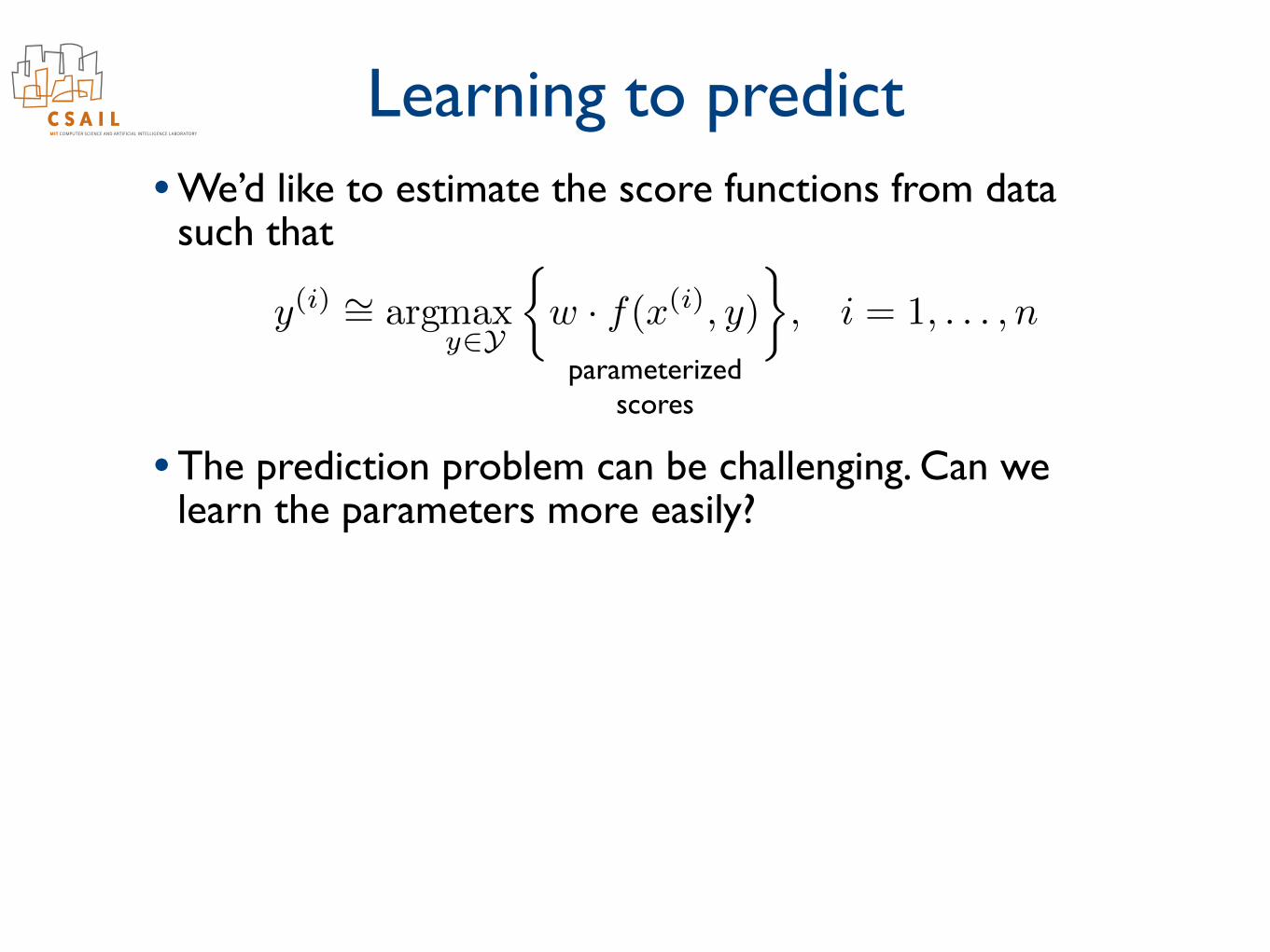
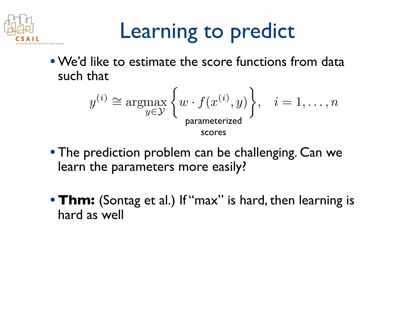
Learning to predict• We’d like to estimate the score functions from data
such that
• The prediction problem can be challenging. Can we learn the parameters more easily?
parameterizedscores
y
(i) ⇠=
argmax
y2Y
⇢w · f(x(i)
, y)
�, i = 1, . . . , n
Learning to predict• We’d like to estimate the score functions from data
such that
• The prediction problem can be challenging. Can we learn the parameters more easily?
• Thm: (Sontag et al.) If “max” is hard, then learning is hard as well
parameterizedscores
y
(i) ⇠=
argmax
y2Y
⇢w · f(x(i)
, y)
�, i = 1, . . . , n
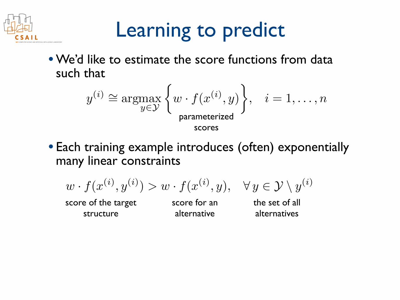
Learning to predict• We’d like to estimate the score functions from data
such that
• Each training example introduces (often) exponentially many linear constraints
parameterizedscores
y
(i) ⇠=
argmax
y2Y
⇢w · f(x(i)
, y)
�, i = 1, . . . , n
w · f(x(i), y
(i)) > w · f(x(i), y), 8 y 2 Y \ y(i)
score of the target structure
score for an alternative
the set of all alternatives
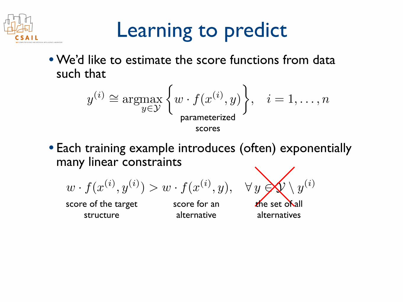
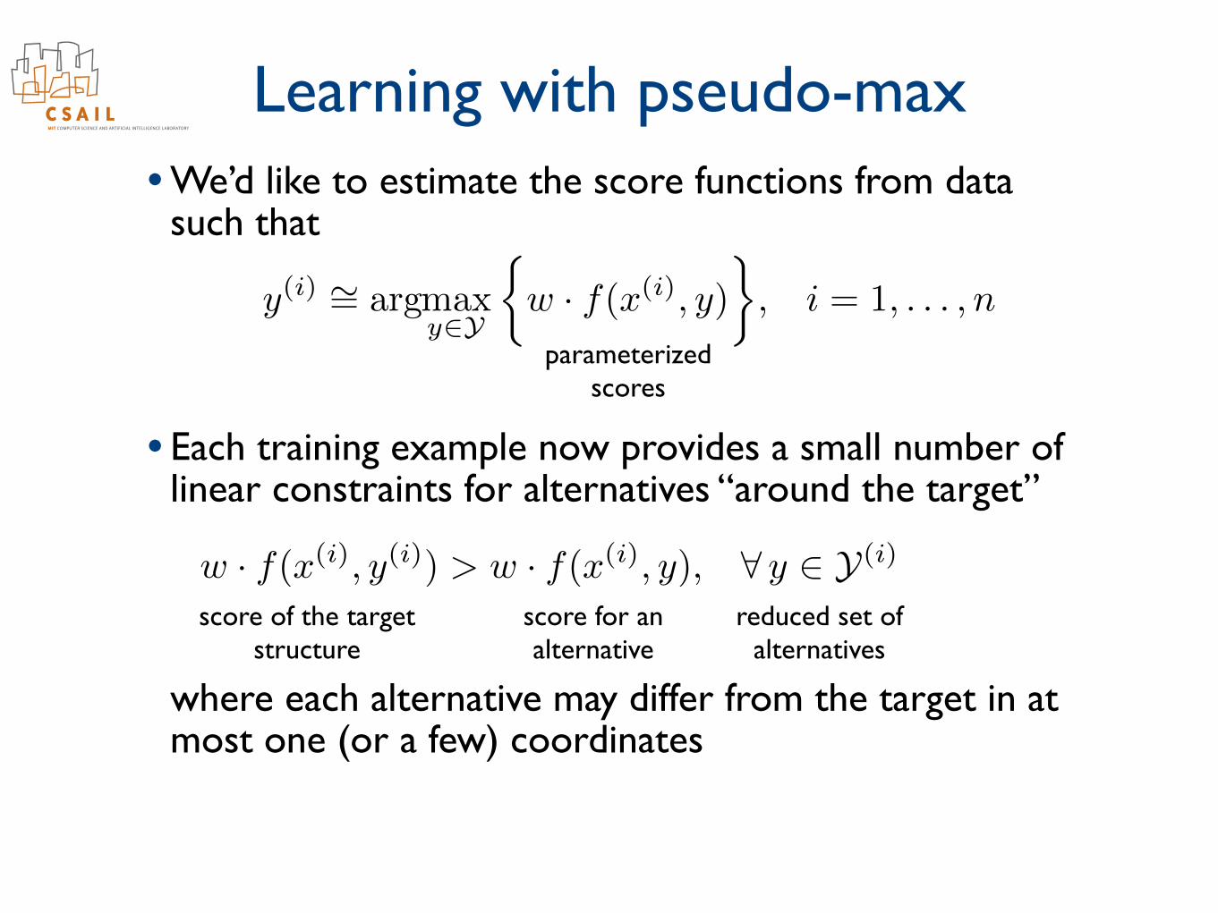
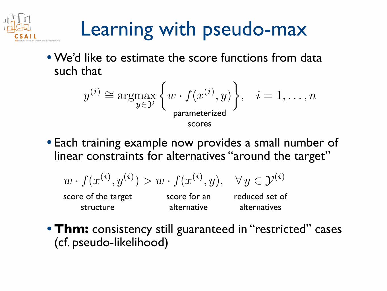
Learning with pseudo-max• We’d like to estimate the score functions from data
such that
• Each training example now provides a small number of linear constraints for alternatives “around the target”
where each alternative may differ from the target in at most one (or a few) coordinates
parameterizedscores
y
(i) ⇠=
argmax
y2Y
⇢w · f(x(i)
, y)
�, i = 1, . . . , n
score of the target structure
score for an alternative
w · f(x(i), y
(i)) > w · f(x(i), y), 8 y 2 Y(i)
reduced set of alternatives
Learning with pseudo-max• We’d like to estimate the score functions from data
such that
• Each training example now provides a small number of linear constraints for alternatives “around the target”
• Thm: consistency still guaranteed in “restricted” cases (cf. pseudo-likelihood)
parameterizedscores
y
(i) ⇠=
argmax
y2Y
⇢w · f(x(i)
, y)
�, i = 1, . . . , n
score of the target structure
score for an alternative
w · f(x(i), y
(i)) > w · f(x(i), y), 8 y 2 Y(i)
reduced set of alternatives
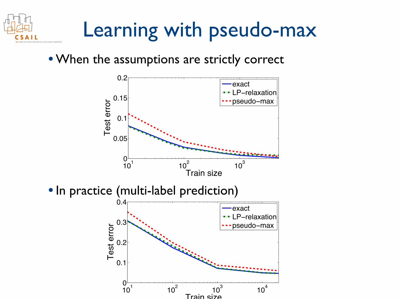
Learning with pseudo-max• When the assumptions are strictly correct
• In practice (multi-label prediction)
101 102 103 1040
0.1
0.2
0.3
0.4
Train size
Test
erro
r
exactLP−relaxationpseudo−max
101 102 103 1040
0.1
0.2
0.3
0.4
Train size
Test
erro
r
exactLP−relaxationpseudo−max
101 102 103 1040
0.1
0.2
0.3
0.4
Train size
Test
erro
r
exactLP−relaxationpseudo−max
101 102 103 1040
0.1
0.2
0.3
0.4
Train size
Test
erro
r
exactLP−relaxationpseudo−max
101 102 1030
0.05
0.1
0.15
0.2
Train size
Test
erro
r
exactLP−relaxationpseudo−max
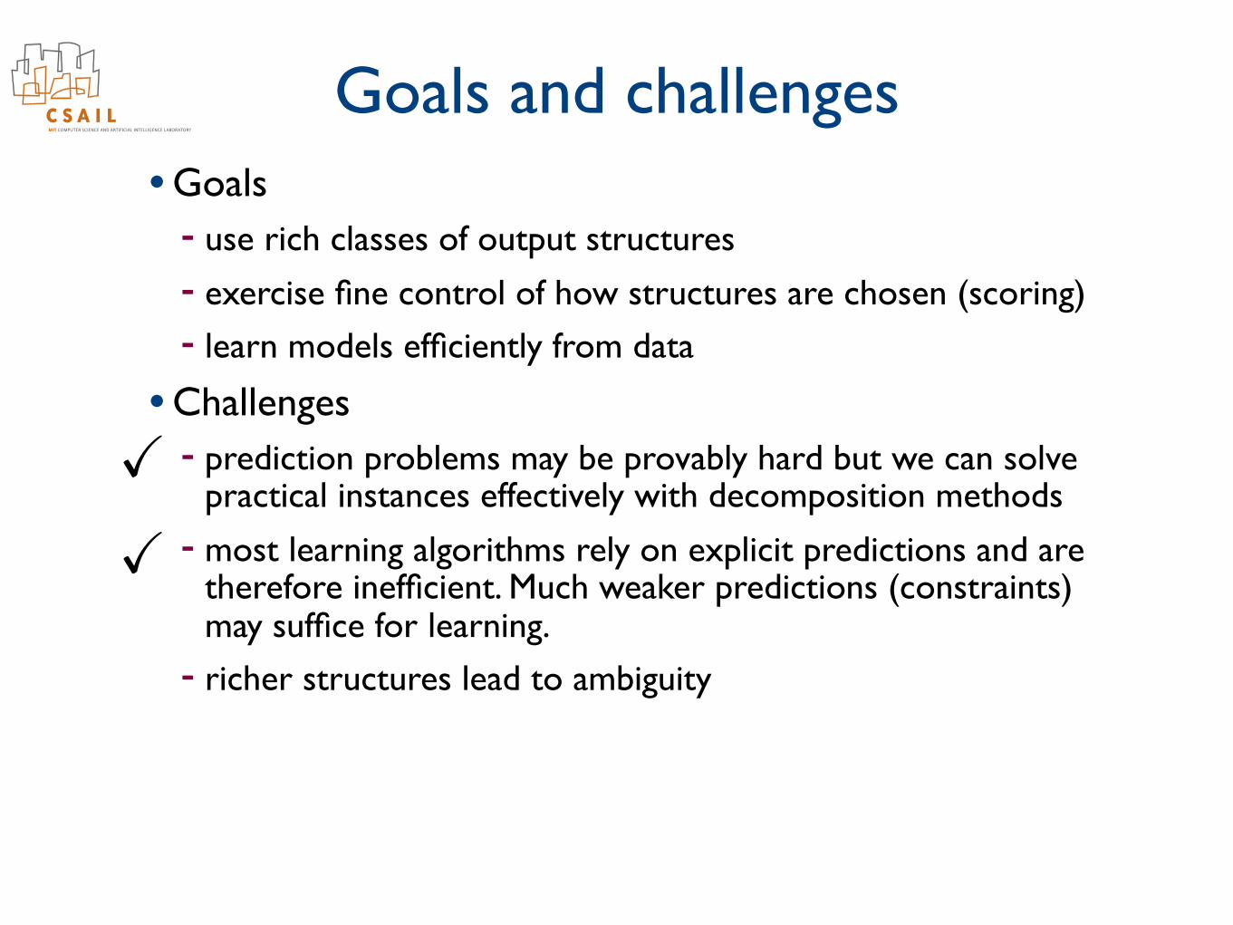
Goals and challenges• Goals
- use rich classes of output structures- exercise fine control of how structures are chosen (scoring)- learn models efficiently from data
• Challenges- prediction problems may be provably hard but we can solve
practical instances effectively with decomposition methods- most learning algorithms rely on explicit predictions and are
therefore inefficient. Much weaker predictions (constraints) may suffice for learning.
- richer structures lead to ambiguity
XX
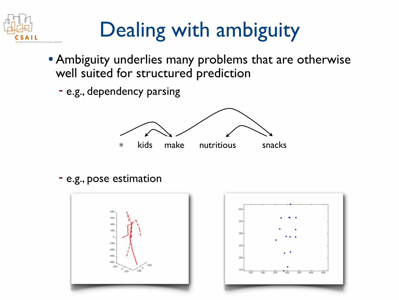
Dealing with ambiguity• Ambiguity underlies many problems that are otherwise
well suited for structured prediction- e.g., dependency parsing
- e.g., pose estimation
kids make nutritious snacks*
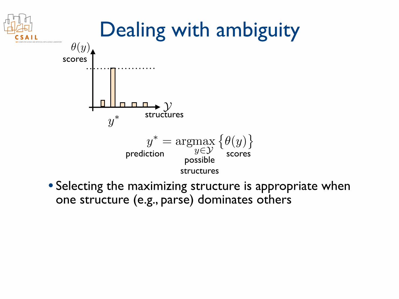
Dealing with ambiguity
• Selecting the maximizing structure is appropriate when one structure (e.g., parse) dominates others
Ystructures
scores
scorespredictionpossible
structures
y⇤
✓(y)
y⇤ = argmax
y2Y
�✓(y)
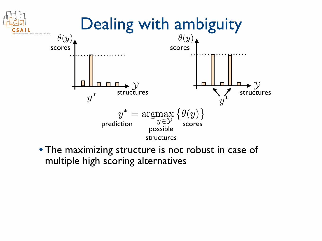
Dealing with ambiguity
• The maximizing structure is not robust in case of multiple high scoring alternatives
Y Ystructures structures
scorespredictionpossible
structures
y⇤ y⇤
y⇤ = argmax
y2Y
�✓(y)
✓(y) ✓(y)scores scores
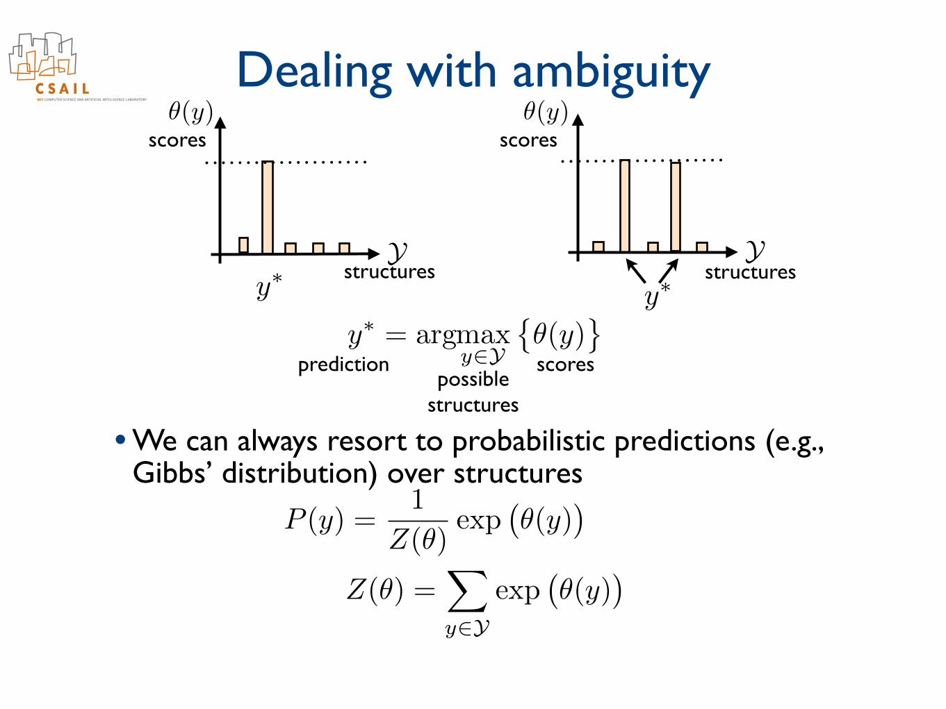
Dealing with ambiguity
• We can always resort to probabilistic predictions (e.g., Gibbs’ distribution) over structures
scorespredictionpossible
structures
P (y) =1
Z(✓)exp
�✓(y)
�
Z(✓) =X
y2Yexp
�✓(y)
�
y⇤ = argmax
y2Y
�✓(y)
Y Ystructures structures
y⇤ y⇤
✓(y) ✓(y)scores scores
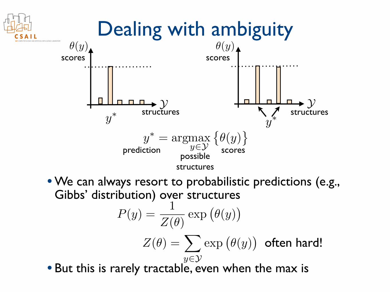
Dealing with ambiguity
• We can always resort to probabilistic predictions (e.g., Gibbs’ distribution) over structures
• But this is rarely tractable, even when the max is
scorespredictionpossible
structures
P (y) =1
Z(✓)exp
�✓(y)
�
Z(✓) =X
y2Yexp
�✓(y)
�
y⇤ = argmax
y2Y
�✓(y)
Y Ystructures structures
y⇤ y⇤
✓(y) ✓(y)scores scores
often hard!

Perturbed Max
• We can induce probabilistic predictions by maximizing randomly perturbed scores- little effect when the maximizing structure is “evident”
perturbed scorespredictionpossible
structures
Ystructures
y⇤
✓(y)scores
y⇤ = argmax
y2Y
�✓(y) + �(y)
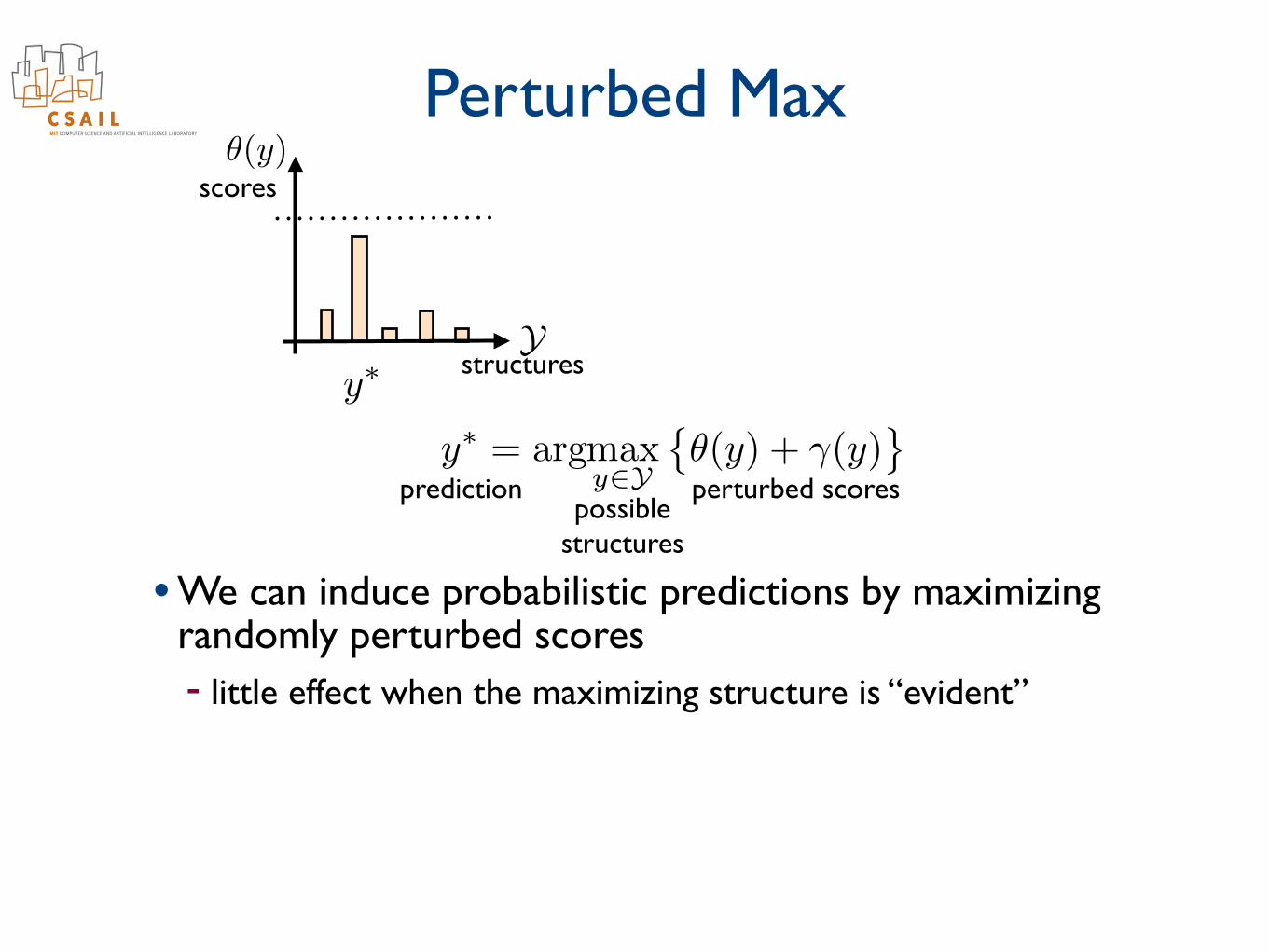
Perturbed Max
• We can induce probabilistic predictions by maximizing randomly perturbed scores- little effect when the maximizing structure is “evident”
perturbed scorespredictionpossible
structures
Ystructures
y⇤
✓(y)scores
y⇤ = argmax
y2Y
�✓(y) + �(y)
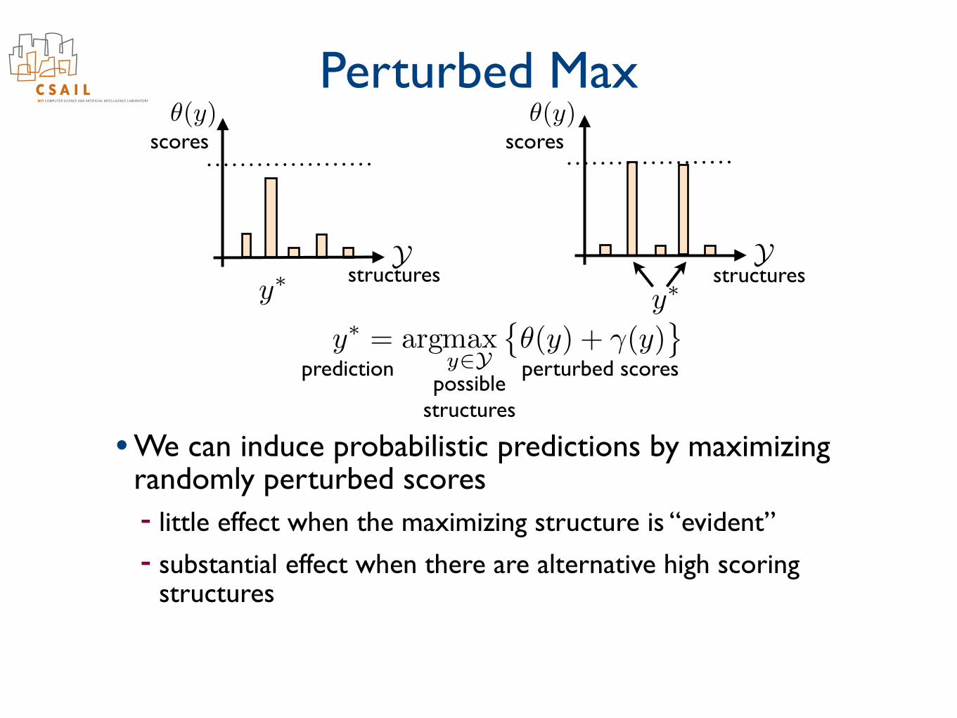
Perturbed Max
• We can induce probabilistic predictions by maximizing randomly perturbed scores- little effect when the maximizing structure is “evident”- substantial effect when there are alternative high scoring
structures
perturbed scorespredictionpossible
structures
Ystructures
y⇤
✓(y)scores
y⇤ = argmax
y2Y
�✓(y) + �(y)
Ystructures
y⇤
✓(y)scores
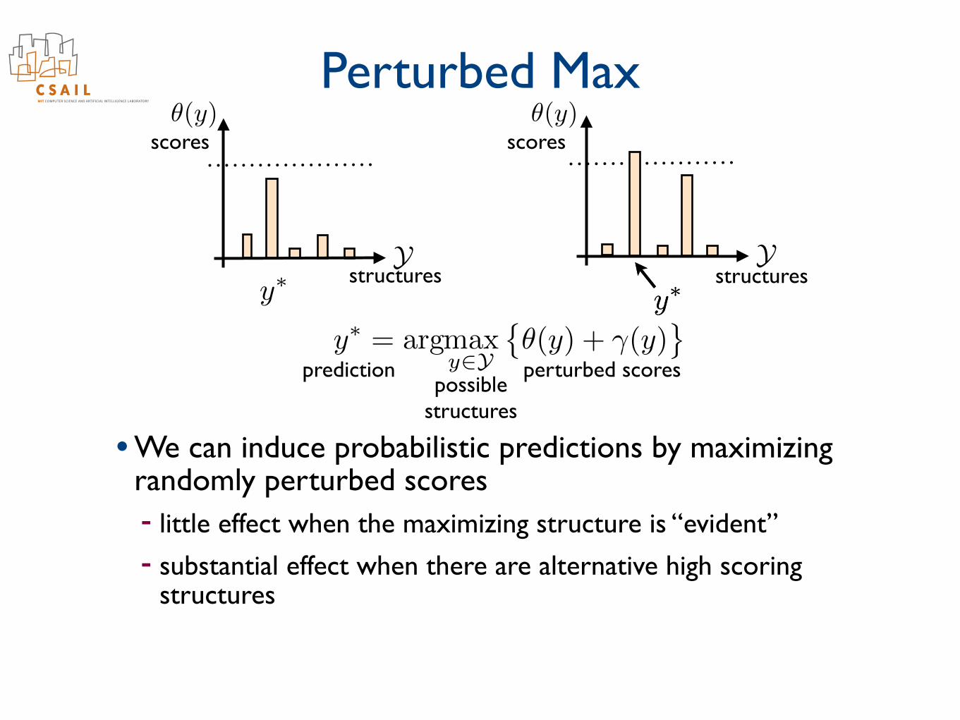
y⇤
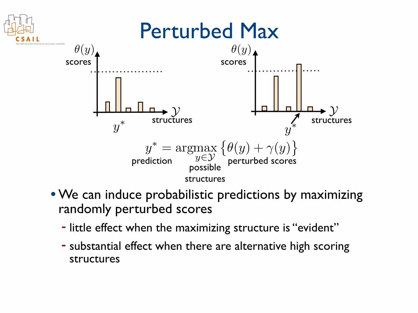
Perturbed Max
• We can induce probabilistic predictions by maximizing randomly perturbed scores- little effect when the maximizing structure is “evident”- substantial effect when there are alternative high scoring
structures
perturbed scorespredictionpossible
structures
Ystructures
y⇤
✓(y)scores
y⇤ = argmax
y2Y
�✓(y) + �(y)
Ystructures
✓(y)scores
y⇤
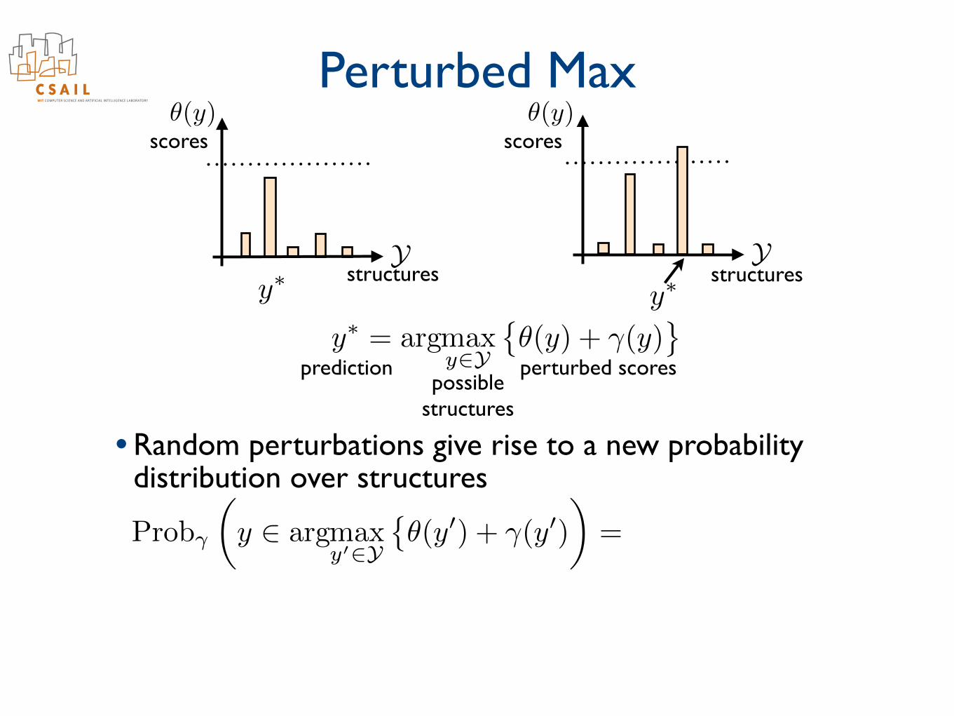
perturbed scorespredictionpossible
structures
Ystructures
y⇤
✓(y)scores
y⇤ = argmax
y2Y
�✓(y) + �(y)
Ystructures
✓(y)scores
y⇤
Prob�
✓y 2 argmax
y02Y
�✓(y0) + �(y0)
◆=
1
Z(✓)exp
�✓(y)
�
• Random perturbations give rise to a new probability distribution over structures
Perturbed Max
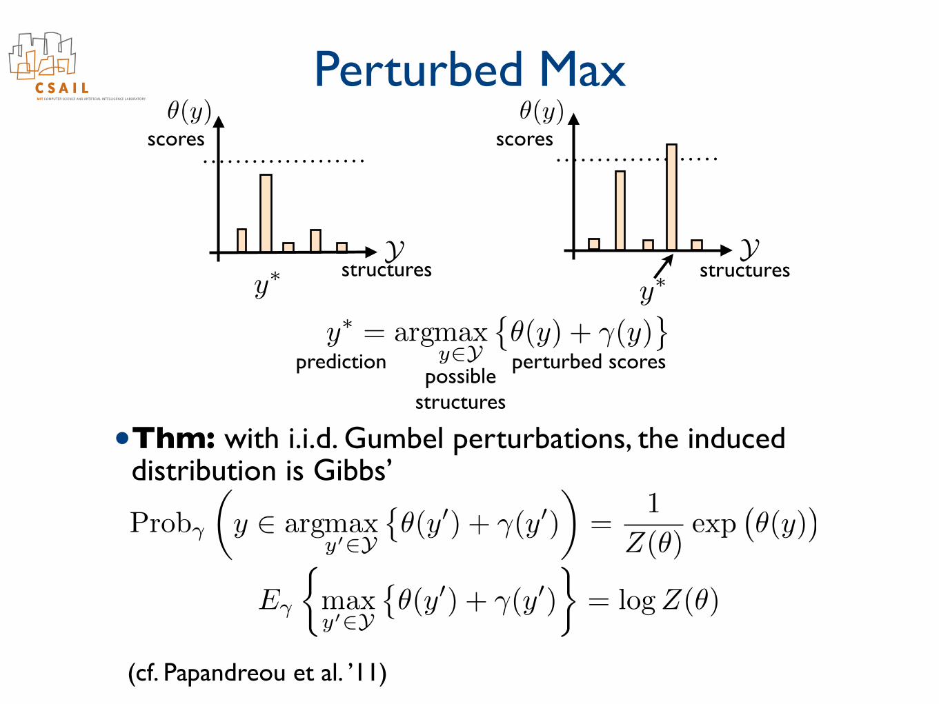
•Thm: with i.i.d. Gumbel perturbations, the induced distribution is Gibbs’
perturbed scorespredictionpossible
structures
Ystructures
y⇤
✓(y)scores
y⇤ = argmax
y2Y
�✓(y) + �(y)
Ystructures
✓(y)scores
y⇤
Prob�
✓y 2 argmax
y02Y
�✓(y0) + �(y0)
◆=
1
Z(✓)exp
�✓(y)
�
(cf. Papandreou et al. ’11)
Perturbed Max
E�
⇢max
y02Y
�✓(y0) + �(y0)
�= logZ(✓)
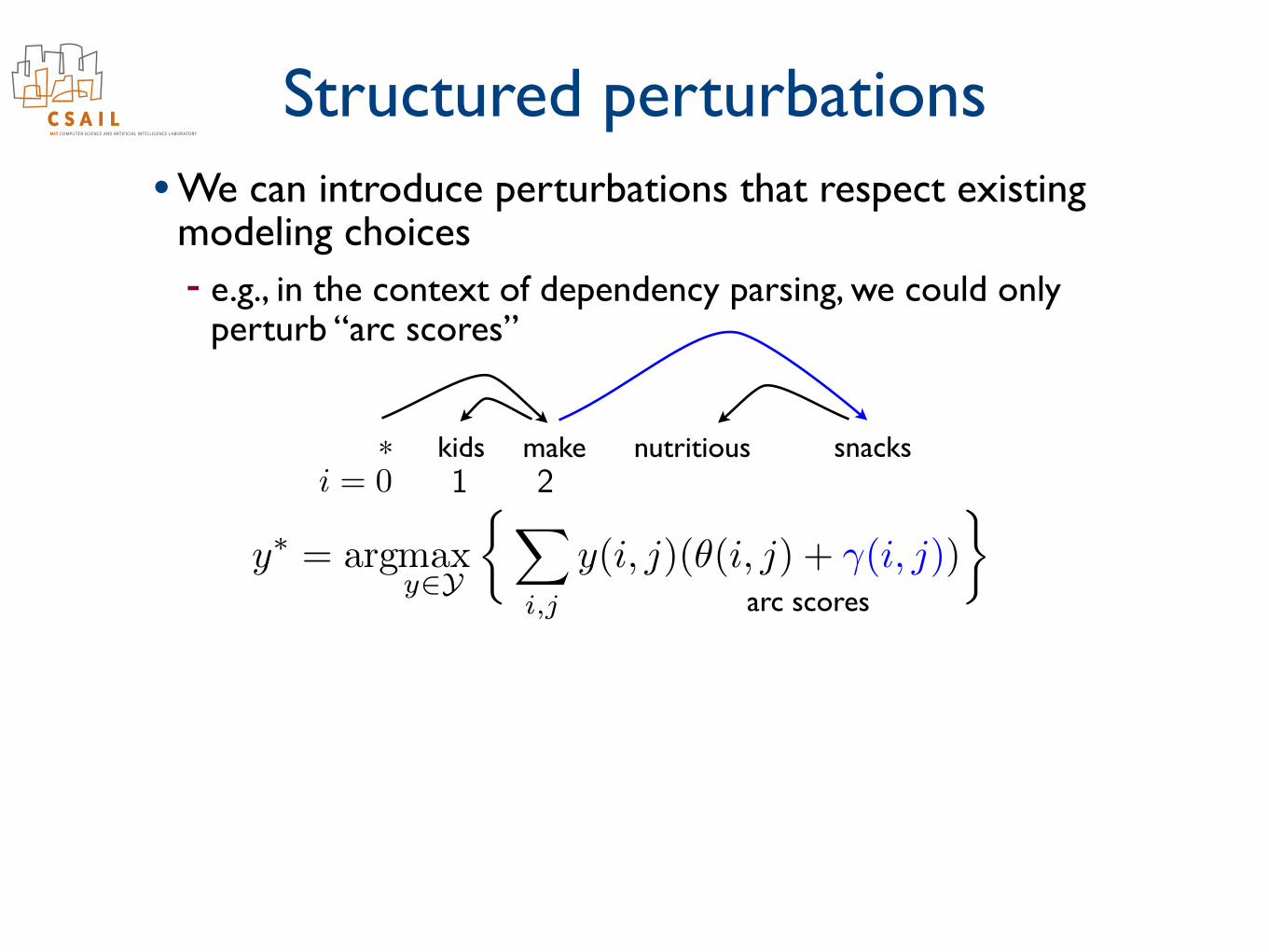
Structured perturbations• We can introduce perturbations that respect existing
modeling choices- e.g., in the context of dependency parsing, we could only
perturb “arc scores”
arc scores
kids make nutritious snacks*i = 0 1 2
y⇤ = argmax
y2Y
⇢X
i,j
y(i, j)(✓(i, j) + �(i, j))
�
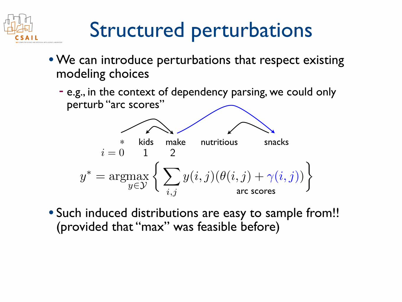
Structured perturbations• We can introduce perturbations that respect existing
modeling choices- e.g., in the context of dependency parsing, we could only
perturb “arc scores”
• Such induced distributions are easy to sample from!! (provided that “max” was feasible before)
arc scores
kids make nutritious snacks*i = 0 1 2
y⇤ = argmax
y2Y
⇢X
i,j
y(i, j)(✓(i, j) + �(i, j))
�
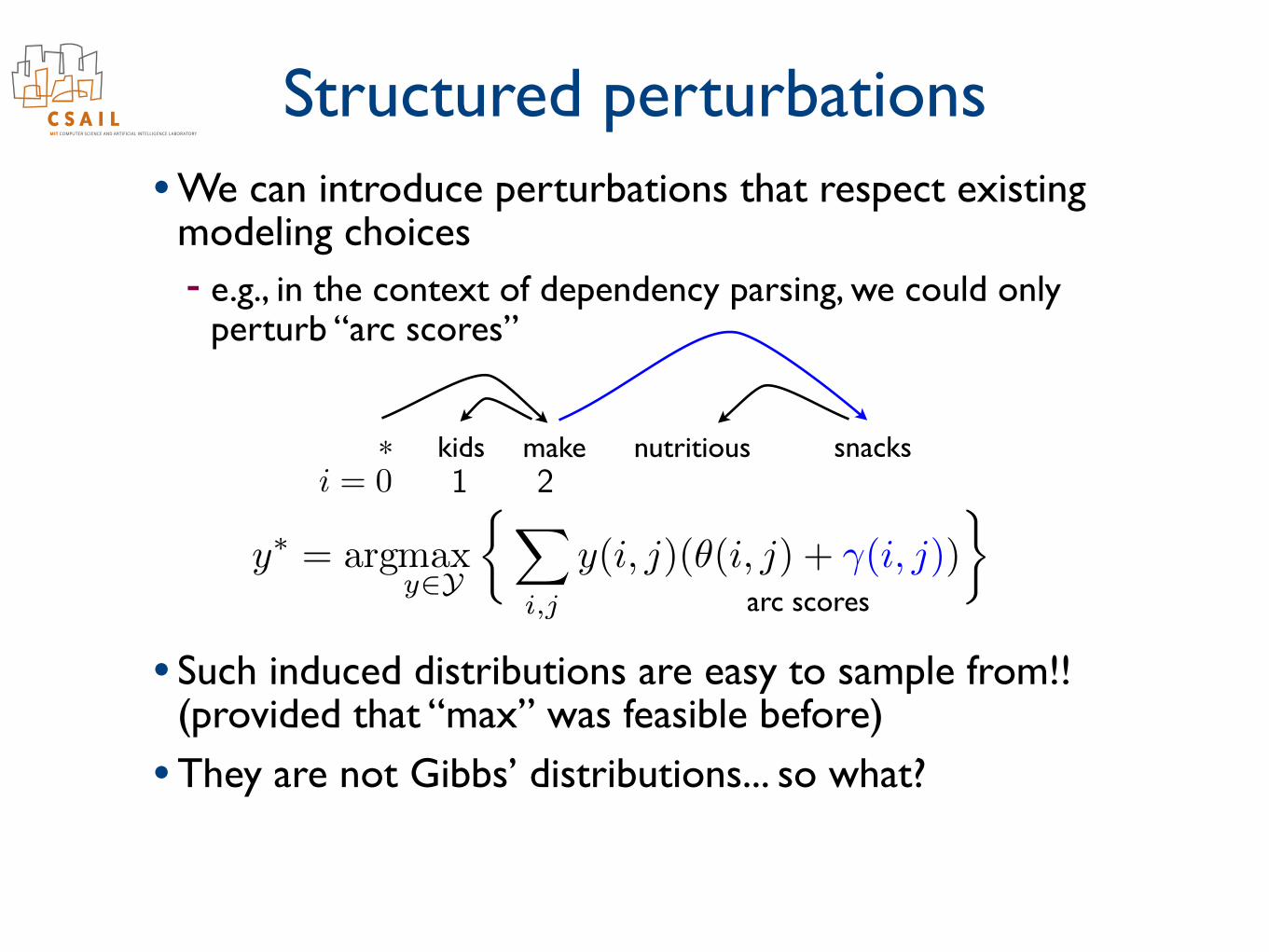
Structured perturbations• We can introduce perturbations that respect existing
modeling choices- e.g., in the context of dependency parsing, we could only
perturb “arc scores”
• Such induced distributions are easy to sample from!! (provided that “max” was feasible before)
• They are not Gibbs’ distributions... so what?
arc scores
kids make nutritious snacks*i = 0 1 2
y⇤ = argmax
y2Y
⇢X
i,j
y(i, j)(✓(i, j) + �(i, j))
�
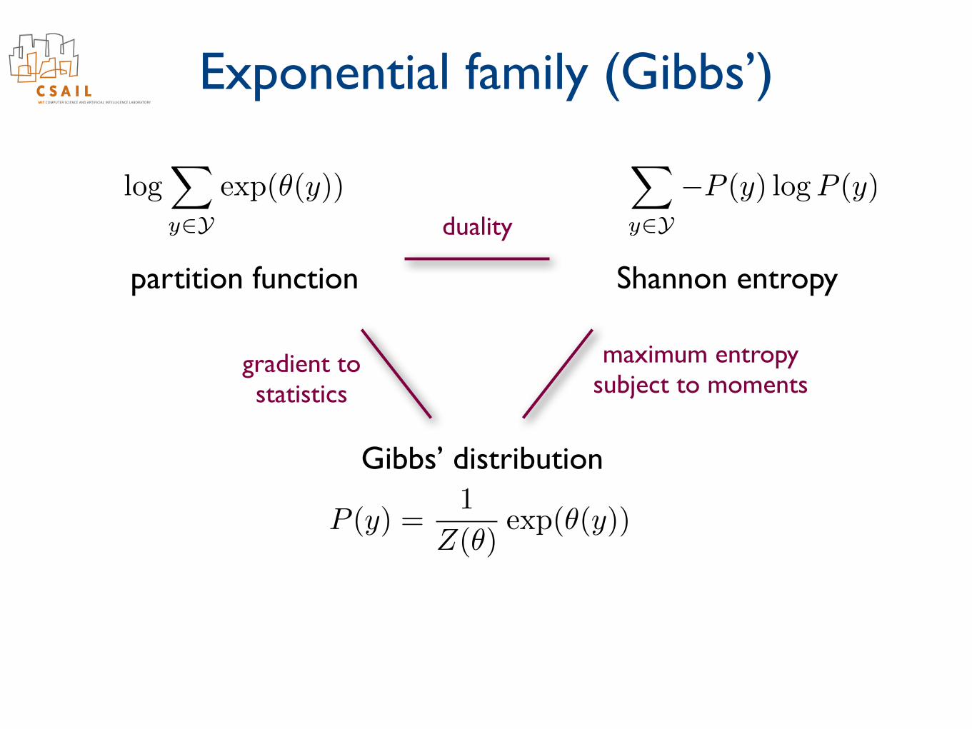
Exponential family (Gibbs’)
partition function Shannon entropy
Gibbs’ distribution
log
X
y2Yexp(✓(y))
X
y2Y�P (y) logP (y)
P (y) =1
Z(✓)exp(✓(y))
duality
gradient tostatistics
maximum entropysubject to moments
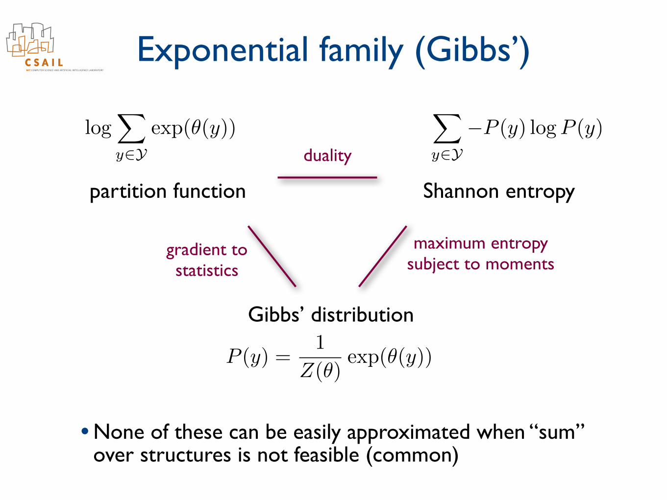
Exponential family (Gibbs’)
partition function Shannon entropy
Gibbs’ distribution
log
X
y2Yexp(✓(y))
X
y2Y�P (y) logP (y)
P (y) =1
Z(✓)exp(✓(y))
duality
gradient tostatistics
maximum entropysubject to moments
• None of these can be easily approximated when “sum” over structures is not feasible (common)
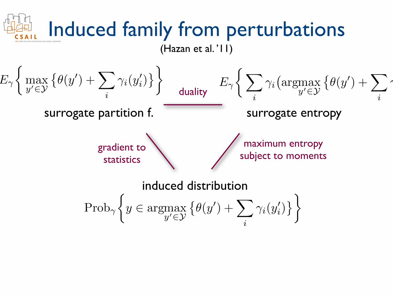
Induced family from perturbations
surrogate partition f. surrogate entropy
induced distribution
duality
gradient tostatistics
maximum entropysubject to moments
E�
⇢max
y02Y
�✓(y0) +
X
i
�i(y0i) �
(Hazan et al. ’11)
Prob�
⇢y 2 argmax
y02Y
�✓(y0) +
X
i
�i(y0i) �
E�
⇢X
i
�i�argmax
y02Y
�✓(y0) +
X
i
�i(y0i) ��
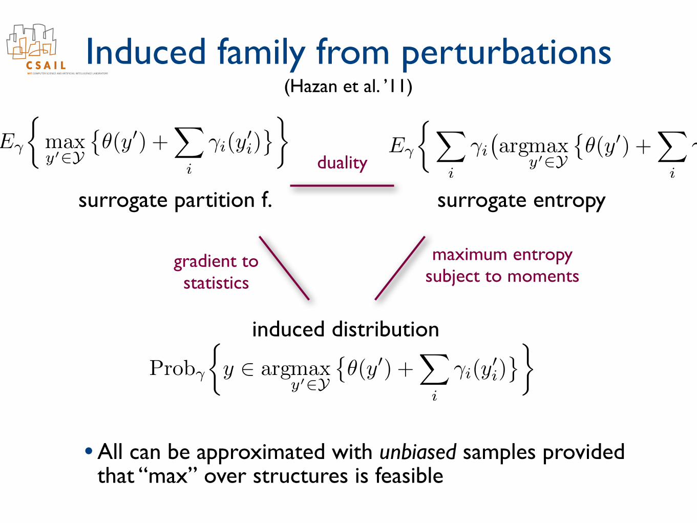
• All can be approximated with unbiased samples provided that “max” over structures is feasible
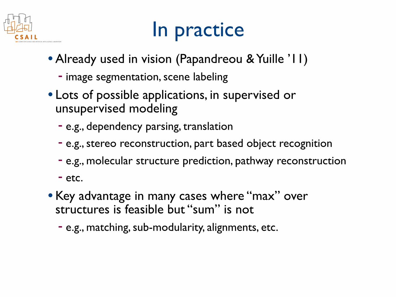
In practice• Already used in vision (Papandreou & Yuille ’11)
- image segmentation, scene labeling
• Lots of possible applications, in supervised or unsupervised modeling- e.g., dependency parsing, translation- e.g., stereo reconstruction, part based object recognition- e.g., molecular structure prediction, pathway reconstruction- etc.
• Key advantage in many cases where “max” over structures is feasible but “sum” is not- e.g., matching, sub-modularity, alignments, etc.
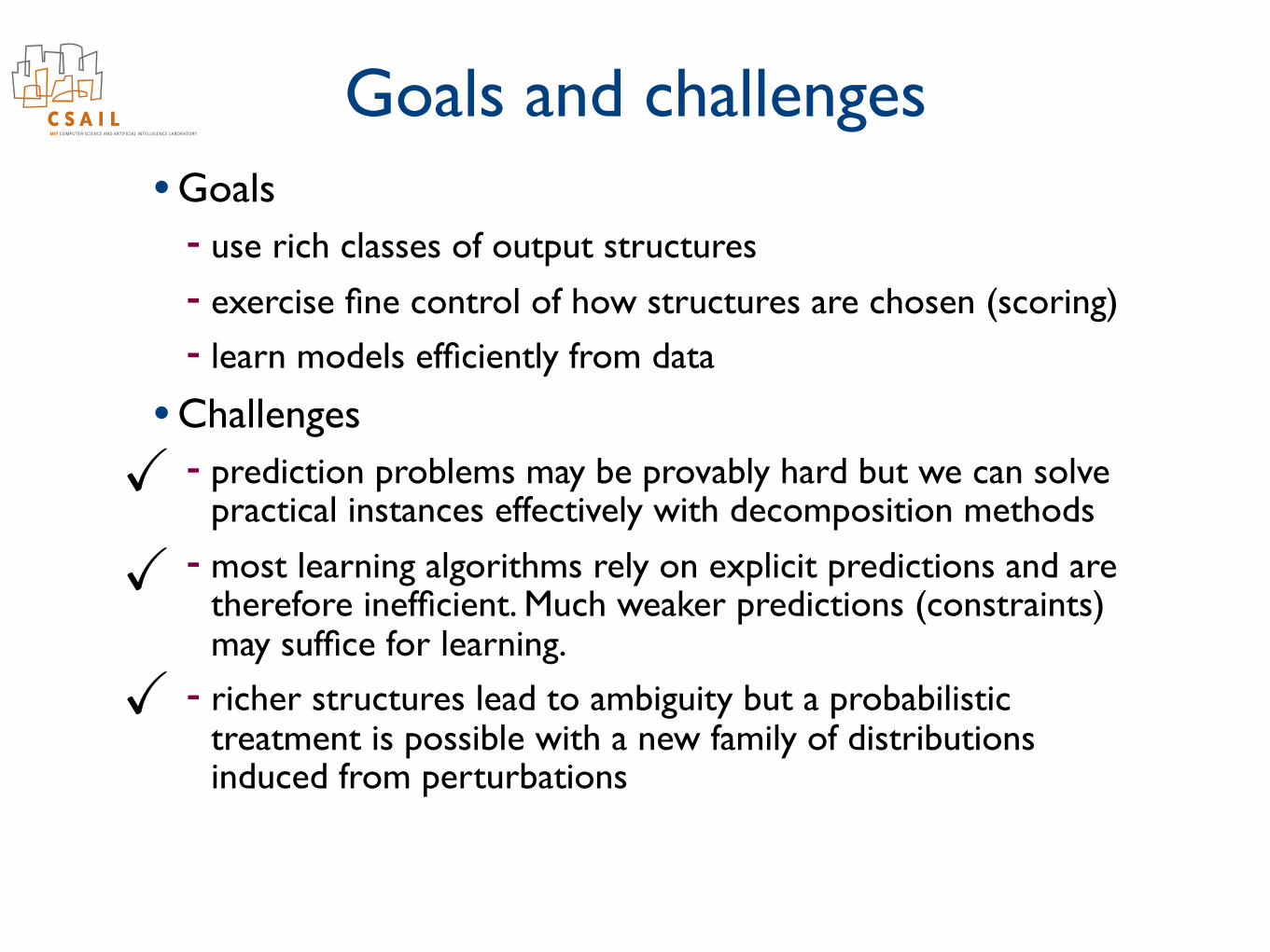
Goals and challenges• Goals
- use rich classes of output structures- exercise fine control of how structures are chosen (scoring)- learn models efficiently from data
• Challenges- prediction problems may be provably hard but we can solve
practical instances effectively with decomposition methods- most learning algorithms rely on explicit predictions and are
therefore inefficient. Much weaker predictions (constraints) may suffice for learning.
- richer structures lead to ambiguity but a probabilistic treatment is possible with a new family of distributions induced from perturbations
XX
X