Embed Size (px)
Citation preview
10
A Survey of Online Failure Prediction Methods
FELIX SALFNER, MAREN LENK, and MIROSLAW MALEK
Humboldt-Universitat zu Berlin
With the ever-growing complexity and dynamicity of computer systems, proactive fault management is aneffective approach to enhancing availability. Online failure prediction is the key to such techniques. In con-trast to classical reliability methods, online failure prediction is based on runtime monitoring and a varietyof models and methods that use the current state of a system and, frequently, the past experience as well.This survey describes these methods. To capture the wide spectrum of approaches concerning this area, ataxonomy has been developed, whose different approaches are explained and major concepts are describedin detail.
Categories and Subject Descriptors: C.4 [Performance of Systems]: Reliability, availability, and serviceabil-ity; Fault tolerance; D.2.5 [Software Engineering]: Testing and Debugging—Error handling and recovery
General Terms: Algorithms, Reliability
Additional Key Words and Phrases: Error, failure prediction, fault, prediction metrics, runtime monitoring
ACM Reference Format:Salfner, F., Lenk, M., and Malek, M. 2010. A survey of online failure prediction methods. ACM Comput. Surv.42, 3, Article 10 (March 2010), 42 pages.DOI = 10.1145/1670679.1670680 http://doi.acm.org/10.1145/1670679.1670680
1. INTRODUCTION
Predicting the future has fascinated people from the beginning of time. Several millionsof people work on prediction daily: astrologers, meteorologists, politicians, pollsters,stock analysts, and doctors, as well as computer scientists and engineers. As computerscientists, we focus on the prediction of computer system failures, a topic that hasattracted interest for more than 30 years. However, what is understood by the termfailure prediction varies among research communities and has also changed over thedecades.
As computer systems are growing more and more complex, they are also changingdynamically due to the mobility of devices, changing execution environments, frequentupdates and upgrades, online repairs, the addition and removal of system components,and the system/network complexity itself. Classical reliability theory and conventional
This research was supported in part by Intel Corporation and by German Research Foundation.Authors’ addresses: Department of Computer Science, Humboldt-Universitat zu Berlin, Unter den Linden6, 10099 Berlin, Germany; email: {salfner,lenk,malek}@informatik.hu-berlin.de.Permission to make digital or hard copies of part or all of this work for personal or classroom use is grantedwithout fee provided that copies are not made or distributed for profit or commercial advantage and thatcopies show this notice on the first page or initial screen of a display along with the full citation. Copyrights forcomponents of this work owned by others than ACM must be honored. Abstracting with credit is permitted.To copy otherwise, to republish, to post on servers, to redistribute to lists, or to use any component of thiswork in other works requires prior specific permission and/or a fee. Permissions may be requested fromPublications Dept., ACM, Inc., 2 Penn Plaza, Suite 701, New York, NY 10121-0701 USA, fax +1 (212) 869-0481, or [email protected]©2010 ACM 0360-0300/2010/03-ART10 $10.00
DOI 10.1145/1670679.1670680 http://doi.acm.org/10.1145/1670679.1670680
ACM Computing Surveys, Vol. 42, No. 3, Article 10, Publication date: March 2010.
10:2 F. Salfner et al.
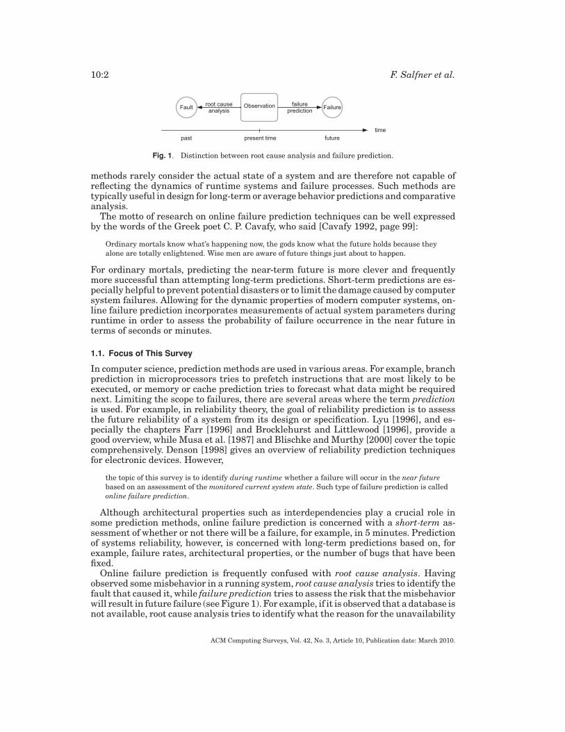
Fig. 1. Distinction between root cause analysis and failure prediction.
methods rarely consider the actual state of a system and are therefore not capable ofreflecting the dynamics of runtime systems and failure processes. Such methods aretypically useful in design for long-term or average behavior predictions and comparativeanalysis.
The motto of research on online failure prediction techniques can be well expressedby the words of the Greek poet C. P. Cavafy, who said [Cavafy 1992, page 99]:
Ordinary mortals know what’s happening now, the gods know what the future holds because theyalone are totally enlightened. Wise men are aware of future things just about to happen.
For ordinary mortals, predicting the near-term future is more clever and frequentlymore successful than attempting long-term predictions. Short-term predictions are es-pecially helpful to prevent potential disasters or to limit the damage caused by computersystem failures. Allowing for the dynamic properties of modern computer systems, on-line failure prediction incorporates measurements of actual system parameters duringruntime in order to assess the probability of failure occurrence in the near future interms of seconds or minutes.
1.1. Focus of This Survey
In computer science, prediction methods are used in various areas. For example, branchprediction in microprocessors tries to prefetch instructions that are most likely to beexecuted, or memory or cache prediction tries to forecast what data might be requirednext. Limiting the scope to failures, there are several areas where the term predictionis used. For example, in reliability theory, the goal of reliability prediction is to assessthe future reliability of a system from its design or specification. Lyu [1996], and es-pecially the chapters Farr [1996] and Brocklehurst and Littlewood [1996], provide agood overview, while Musa et al. [1987] and Blischke and Murthy [2000] cover the topiccomprehensively. Denson [1998] gives an overview of reliability prediction techniquesfor electronic devices. However,
the topic of this survey is to identify during runtime whether a failure will occur in the near futurebased on an assessment of the monitored current system state. Such type of failure prediction is calledonline failure prediction.
Although architectural properties such as interdependencies play a crucial role insome prediction methods, online failure prediction is concerned with a short-term as-sessment of whether or not there will be a failure, for example, in 5 minutes. Predictionof systems reliability, however, is concerned with long-term predictions based on, forexample, failure rates, architectural properties, or the number of bugs that have beenfixed.
Online failure prediction is frequently confused with root cause analysis. Havingobserved some misbehavior in a running system, root cause analysis tries to identify thefault that caused it, while failure prediction tries to assess the risk that the misbehaviorwill result in future failure (see Figure 1). For example, if it is observed that a database isnot available, root cause analysis tries to identify what the reason for the unavailability
ACM Computing Surveys, Vol. 42, No. 3, Article 10, Publication date: March 2010.
Survey of Online Failure Prediction Methods 10:3
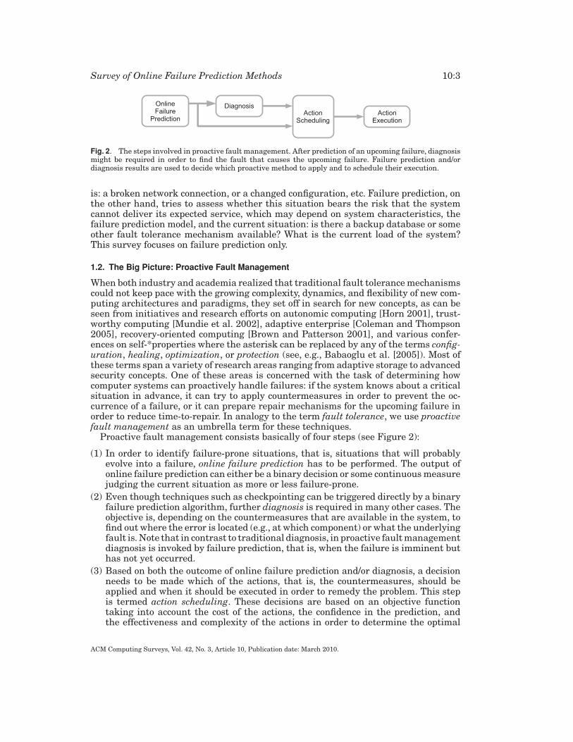
Fig. 2. The steps involved in proactive fault management. After prediction of an upcoming failure, diagnosismight be required in order to find the fault that causes the upcoming failure. Failure prediction and/ordiagnosis results are used to decide which proactive method to apply and to schedule their execution.
is: a broken network connection, or a changed configuration, etc. Failure prediction, onthe other hand, tries to assess whether this situation bears the risk that the systemcannot deliver its expected service, which may depend on system characteristics, thefailure prediction model, and the current situation: is there a backup database or someother fault tolerance mechanism available? What is the current load of the system?This survey focuses on failure prediction only.
1.2. The Big Picture: Proactive Fault Management
When both industry and academia realized that traditional fault tolerance mechanismscould not keep pace with the growing complexity, dynamics, and flexibility of new com-puting architectures and paradigms, they set off in search for new concepts, as can beseen from initiatives and research efforts on autonomic computing [Horn 2001], trust-worthy computing [Mundie et al. 2002], adaptive enterprise [Coleman and Thompson2005], recovery-oriented computing [Brown and Patterson 2001], and various confer-ences on self-*properties where the asterisk can be replaced by any of the terms config-uration, healing, optimization, or protection (see, e.g., Babaoglu et al. [2005]). Most ofthese terms span a variety of research areas ranging from adaptive storage to advancedsecurity concepts. One of these areas is concerned with the task of determining howcomputer systems can proactively handle failures: if the system knows about a criticalsituation in advance, it can try to apply countermeasures in order to prevent the oc-currence of a failure, or it can prepare repair mechanisms for the upcoming failure inorder to reduce time-to-repair. In analogy to the term fault tolerance, we use proactivefault management as an umbrella term for these techniques.
Proactive fault management consists basically of four steps (see Figure 2):
(1) In order to identify failure-prone situations, that is, situations that will probablyevolve into a failure, online failure prediction has to be performed. The output ofonline failure prediction can either be a binary decision or some continuous measurejudging the current situation as more or less failure-prone.
(2) Even though techniques such as checkpointing can be triggered directly by a binaryfailure prediction algorithm, further diagnosis is required in many other cases. Theobjective is, depending on the countermeasures that are available in the system, tofind out where the error is located (e.g., at which component) or what the underlyingfault is. Note that in contrast to traditional diagnosis, in proactive fault managementdiagnosis is invoked by failure prediction, that is, when the failure is imminent buthas not yet occurred.
(3) Based on both the outcome of online failure prediction and/or diagnosis, a decisionneeds to be made which of the actions, that is, the countermeasures, should beapplied and when it should be executed in order to remedy the problem. This stepis termed action scheduling. These decisions are based on an objective functiontaking into account the cost of the actions, the confidence in the prediction, andthe effectiveness and complexity of the actions in order to determine the optimal
ACM Computing Surveys, Vol. 42, No. 3, Article 10, Publication date: March 2010.
10:4 F. Salfner et al.
tradeoff. For example, in order to trigger a rather costly technique, the schedulershould be almost sure about an upcoming failure, whereas for a less expensiveaction less confidence in the correctness of failure prediction is required. Candeaet al. [2004] have examined this relationship quantitatively. They showed that shortrestart times (microreboots) allow for a higher false positive rate in comparison toslower restarts (process restarts).1 Many emerging concepts such as the policiesused in IBM’s autonomic manager relate to action scheduling as well.
(4) The last step in proactive fault management is the actual execution of actions. Chal-lenges for action execution include online reconfiguration of globally distributedsystems, data synchronization of distributed data centers, and many more.
In summary, accurate online failure prediction is only the prerequisite in the chainand each of the remaining three steps constitutes a whole field of research of its own.Not devaluing the efforts that have been made in the other fields, this survey providesan overview of online failure prediction.
In order to build a proactive fault management solution that is able to boost sys-tem dependability by up to an order of magnitude, the best techniques from all fourfields for the given surrounding conditions have to be combined. However, this re-quires comparability of approaches, which can only be achieved if two conditions aremet:
—a set of standard quality evaluation metrics is available, and
—publicly available reference data sets can be accessed.
Regarding reference data sets, a first initiative was started in 2006 by Carnegie MellonUniversity, called the Computer Failure Data Repository,2 that publicly provides de-tailed failure data from a variety of large production systems such as high-performanceclusters at the Lawrence Livermore National Laboratory.
Regarding standard metrics, this survey provides the first step by presenting anddiscussing major metrics for the evaluation of online failure prediction approaches.
1.3. Outline
This article is a survey on failure prediction methods that have been used to predictfailures of computer systems online, that is, those based on the current system state.Starting from a definition of the basic terms such as errors, failures, and lead time(Section 2), established metrics to investigate the quality of failure prediction algo-rithms are reviewed in Section 3. In order to structure the wide spectrum of meth-ods, a taxonomy is introduced in Section 4 and almost 50 online failure predictionapproaches are surveyed in Section 5. A comprehensive list of all failure predictionmethods together with demonstrated and potential applications is provided in the sum-mary and conclusions (Section 6). In order to give further insight into online failureprediction approaches, selected representative methods are described in greater de-tail in the electronic appendix available in the ACM Digital Library. In Appendix A atable of the selected methods is provided, and in Appendices B–K the techniques arediscussed.
1Although in Candea et al. [2004] false positives relate to falsely suspecting a component to be at fault,similar relationships should hold for failure predictions too.2http://cfdr.usenix.org.
ACM Computing Surveys, Vol. 42, No. 3, Article 10, Publication date: March 2010.

Survey of Online Failure Prediction Methods 10:5
2. DEFINITIONS
The aim of online failure prediction is to predict the occurrence of failures during run-time based on the current system state. The following sections provide more precisedefinitions of the terms used throughout this article.
2.1. Faults, Errors, Symptoms, and Failures
Several attempts have been made to get to a precise definition of faults, errors, andfailures, among which are Melliar-Smith and Randell [1977]; Avizienis and Laprie[1986]; Laprie and Kanoun [1996]; and IEC: International Technical Comission [2002];Siewiorek and Swarz [1998], page 22; and most recently Avizienis et al. [2004]. Sincethe latter seems to have broad acceptance, its definitions are used in this article, withsome additional extensions and interpretations.
—A failure is defined as “an event that occurs when the delivered service deviates fromcorrect service.” The main point here is that a failure refers to misbehavior that canbe observed by the user, which can either be a human or another computer system.Things may go wrong inside the system, but as long as the problem does not resultin incorrect output (including the case where there is no output at all) there is nofailure.
—The situation when “things go wrong” in the system can be formalized as the situationwhen the system’s state deviates from the correct state, which is called an error.Hence, “an error is the part of the total state of the system that may lead to itssubsequent service failure.”
—Finally, faults are the adjudged or hypothesized cause of an error—the root cause ofan error. In most cases, faults remain dormant for some time and, once they becomeactive, they cause an incorrect system state, which is an error. That is why errors arealso called manifestations of faults. Several classifications of faults have been pro-posed in the literature, among which the distinction between transient, intermittent,and permanent faults [Siewiorek and Swarz 1998, page 22] is best known.
—The definition of an error implies that the activation of a fault leads to an incorrectstate; however, this does not necessarily mean that the system knows about it. Inaddition to the definitions given by Avizienis et al. [2004], we distinguish betweenundetected errors and detected errors: an error remains undetected until an errordetector identifies the incorrect state.
—Besides causing a failure, undetected or detected errors may cause out-of-norm be-havior of system parameters as a side effect. We call this out-of-norm behavior asymptom.3 In the context of software aging, symptoms are similar to aging-relatederrors, as implicitly introduced in Grottke and Trivedi [2007] and explicitly namedin Grottke et al. [2008].
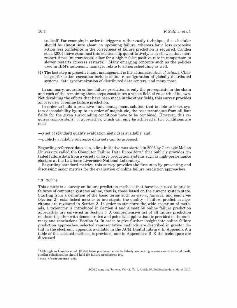
Figure 3 visualizes how a fault can evolve into a failure. Note that there can be anm-to-n mapping between faults, errors, symptoms, and failures: For example, severalfaults may result in one single error or one fault may result in several errors. Thesame holds for errors and failures: some errors result in a failure, some errors do not,and more complicated, some errors only result in a failure under special conditions.As is also indicated in the figure, an undetected error may cause a failure directly ormight even be nondistinguishable from it. Furthermore, errors do not necessarily showsymptoms.
3This should not be confused with Iyer et al. [1986], who used the term symptom for the most significanterrors within an error group.
ACM Computing Surveys, Vol. 42, No. 3, Article 10, Publication date: March 2010.
10:6 F. Salfner et al.
Fig. 3. Interrelations of faults, errors, symptoms, and failures. Encapsulating boxes show the technique bywhich the corresponding flaw can be made visible.
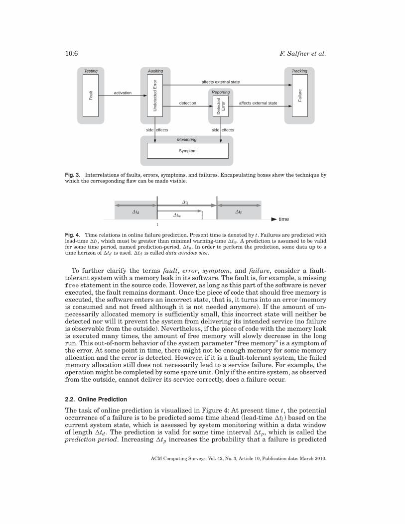
Fig. 4. Time relations in online failure prediction. Present time is denoted by t. Failures are predicted withlead-time �tl , which must be greater than minimal warning-time �tw. A prediction is assumed to be validfor some time period, named prediction-period, �tp. In order to perform the prediction, some data up to atime horizon of �td is used. �td is called data window size.
To further clarify the terms fault, error, symptom, and failure, consider a fault-tolerant system with a memory leak in its software. The fault is, for example, a missingfree statement in the source code. However, as long as this part of the software is neverexecuted, the fault remains dormant. Once the piece of code that should free memory isexecuted, the software enters an incorrect state, that is, it turns into an error (memoryis consumed and not freed although it is not needed anymore). If the amount of un-necessarily allocated memory is sufficiently small, this incorrect state will neither bedetected nor will it prevent the system from delivering its intended service (no failureis observable from the outside). Nevertheless, if the piece of code with the memory leakis executed many times, the amount of free memory will slowly decrease in the longrun. This out-of-norm behavior of the system parameter “free memory” is a symptom ofthe error. At some point in time, there might not be enough memory for some memoryallocation and the error is detected. However, if it is a fault-tolerant system, the failedmemory allocation still does not necessarily lead to a service failure. For example, theoperation might be completed by some spare unit. Only if the entire system, as observedfrom the outside, cannot deliver its service correctly, does a failure occur.
2.2. Online Prediction
The task of online prediction is visualized in Figure 4: At present time t, the potentialoccurrence of a failure is to be predicted some time ahead (lead-time �tl ) based on thecurrent system state, which is assessed by system monitoring within a data windowof length �td . The prediction is valid for some time interval �tp, which is called theprediction period. Increasing �tp increases the probability that a failure is predicted
ACM Computing Surveys, Vol. 42, No. 3, Article 10, Publication date: March 2010.

Survey of Online Failure Prediction Methods 10:7
Table I. Contingency Table(Any failure prediction belongs to one out of four cases: if the prediction algorithm decides in
favor of an upcoming failure, which is called a positive, it results in raising a failure warning. Thisdecision can be right or wrong. If in reality a failure is imminent, the prediction is a true positive. Ifnot, a false positive. Analogously, in case the prediction indicates that the system is running well
(a negative prediction), this prediction may be right (true negative) or wrong (false negative)).True failure True nonfailure Sum
Prediction: failure True positive (TP) False positive (FP) Positives(failure warning) (correct warning) (false warning) (POS)
Prediction: no failure False negative (FN) True negative (TN) Negatives(no failure warning) (missing warning) (correctly no warning) (NEG)
Sum Failures (F ) Nonfailures (NF) Total (N )
correctly.4 On the other hand, if �tp is too large, the prediction is of little use since itis not clear when exactly the failure will occur. Since failure prediction does not makesense if the lead-time is larger than the time the system needs to react in order to avoida failure or to prepare for it, Figure 4 introduces the minimal warning time �tw. Ifthe lead-time were shorter than the warning time, there would not be enough time toperform any preparatory or preventive actions.
3. EVALUATION METRICS
In order to investigate the quality of failure prediction algorithms and to compare theirpotential, it is necessary to specify metrics (figures of merit). It is the goal of failureprediction to predict failures accurately: covering as many failures as possible whileat the same time generating as few false alarms as possible. A perfect failure predic-tion would achieve a one-to-one matching between predicted and true failures. Thissection will introduce several established metrics for the goodness of fit of prediction.Some other metrics have been proposed, for example, the kappa statistic Altman [1991,page 404], but they are rarely used by the community. A more detailed discussion andanalysis of evaluation metrics for online failure prediction can be found in Salfner[2008], Chapter 8.2.
Table I defines four cases: a failure prediction is a true positive if a failure occurswithin the prediction period and a failure warning is raised. If no failure occurs anda warning is given, the prediction is a false positive. If the algorithm fails to predicta true failure, it is a false negative. If no true failure occurs and no failure warning israised, the prediction is a true negative.
3.1. Contingency Table Metrics
The metrics presented here are based on the contingency table (see Table I) andtherefore called contingency table metrics. They are often used in pairs such as pre-cision/recall, true positive rate/false positive rate, sensitivity/specificity, and positivepredictive value/negative predictive value. Table II provides an overview.
In various research areas, different names have been established for the same met-rics. Hence the leftmost column indicates which terms are used in this article, and therightmost column lists additional names.
Precision is defined as the ratio of correctly identified failures to the number of allpredicted failures:
precision = TPTP + FP
. (1)
4For �tp → ∞, simply predicting that a failure will occur would always be 100% correct!
ACM Computing Surveys, Vol. 42, No. 3, Article 10, Publication date: March 2010.
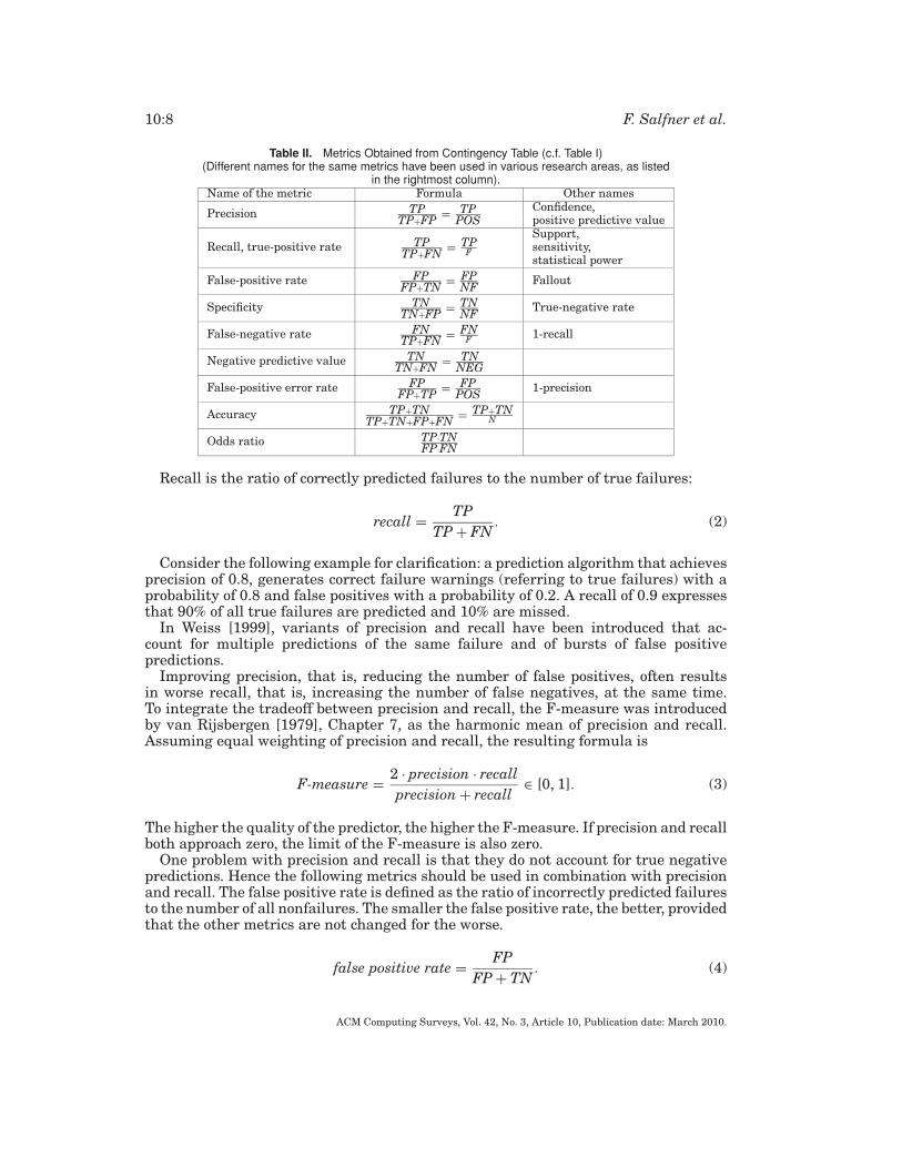
10:8 F. Salfner et al.
Table II. Metrics Obtained from Contingency Table (c.f. Table I)(Different names for the same metrics have been used in various research areas, as listed
in the rightmost column).Name of the metric Formula Other names
Precision TPTP+FP = TP
POSConfidence,positive predictive value
Recall, true-positive rate TPTP+FN = TP
F
Support,sensitivity,statistical power
False-positive rate FPFP+TN = FP
NF Fallout
Specificity TNTN+FP = TN
NF True-negative rate
False-negative rate FNTP+FN = FN
F 1-recall
Negative predictive value TNTN+FN = TN
NEG
False-positive error rate FPFP+TP = FP
POS 1-precision
Accuracy TP+TNTP+TN+FP+FN = TP+TN
N
Odds ratio TP·TNFP·FN
Recall is the ratio of correctly predicted failures to the number of true failures:
recall = TPTP + FN
. (2)
Consider the following example for clarification: a prediction algorithm that achievesprecision of 0.8, generates correct failure warnings (referring to true failures) with aprobability of 0.8 and false positives with a probability of 0.2. A recall of 0.9 expressesthat 90% of all true failures are predicted and 10% are missed.
In Weiss [1999], variants of precision and recall have been introduced that ac-count for multiple predictions of the same failure and of bursts of false positivepredictions.
Improving precision, that is, reducing the number of false positives, often resultsin worse recall, that is, increasing the number of false negatives, at the same time.To integrate the tradeoff between precision and recall, the F-measure was introducedby van Rijsbergen [1979], Chapter 7, as the harmonic mean of precision and recall.Assuming equal weighting of precision and recall, the resulting formula is
F-measure = 2 · precision · recallprecision + recall
∈ [0, 1]. (3)
The higher the quality of the predictor, the higher the F-measure. If precision and recallboth approach zero, the limit of the F-measure is also zero.
One problem with precision and recall is that they do not account for true negativepredictions. Hence the following metrics should be used in combination with precisionand recall. The false positive rate is defined as the ratio of incorrectly predicted failuresto the number of all nonfailures. The smaller the false positive rate, the better, providedthat the other metrics are not changed for the worse.
false positive rate = FPFP + TN
. (4)
ACM Computing Surveys, Vol. 42, No. 3, Article 10, Publication date: March 2010.
Survey of Online Failure Prediction Methods 10:9
Specificity is defined as the ratio of all correctly not raised failure warnings to thenumber of all nonfailures:
specificity = TNFP + TN
= 1 − false positive rate. (5)
The negative predictive value (NPV) is the ratio of all correctly not raised failurewarnings to the number of all not raised warnings:
negative predictive value = TNTN + FN
. (6)
Accuracy is defined as the ratio of all correct predictions to the number of all predic-tions that have been performed:
accuracy = TP + TNTP + FP + FN + TN
. (7)
Due to the fact that failures usually are rare events, accuracy does not appear to be anappropriate metric for failure prediction: a strategy that always classifies the systemto be nonfaulty can achieve excellent accuracy since it is right in most of the cases,although it does not catch any failure (recall is zero).
From this discussion it might be concluded that true negatives are not of interest forthe assessment of failure prediction techniques. This is not necessarily true since thenumber of true negatives can help to assess the impact of a failure prediction approachon the system. Consider the following example: for a given time period including agiven number of failures, two prediction methods do equally well in terms of TP, FP,and FN; hence both achieve the same precision and recall. However, one predictionalgorithm performs 10 times as many predictions as the second since, for example, oneoperates on measurements taken every second and the other on measurements thatare taken only every 10s. The difference between the two methods is reflected only inthe number of TNs and will hence only become visible in metrics that include TNs.The number of true negatives can be determined by counting all predictions that wereperformed when no true failure was imminent and no failure warning was issued as aresult of the prediction.
It should also be pointed out that quality of predictions depends not only on algo-rithms but also on the data window size �td , lead-time �tl , and prediction-period �tp.For example, since it is very unlikely to predict that a failure will occur at one exactpoint in time but only within a certain time interval (prediction period), the number oftrue positives depends on �tp: the longer the prediction period, the more failures arecaptured and hence the number of true positives goes up, which affects, for example,recall. That is why the contingency table should only be determined for one specificcombination of �td , �tp, and �tl .
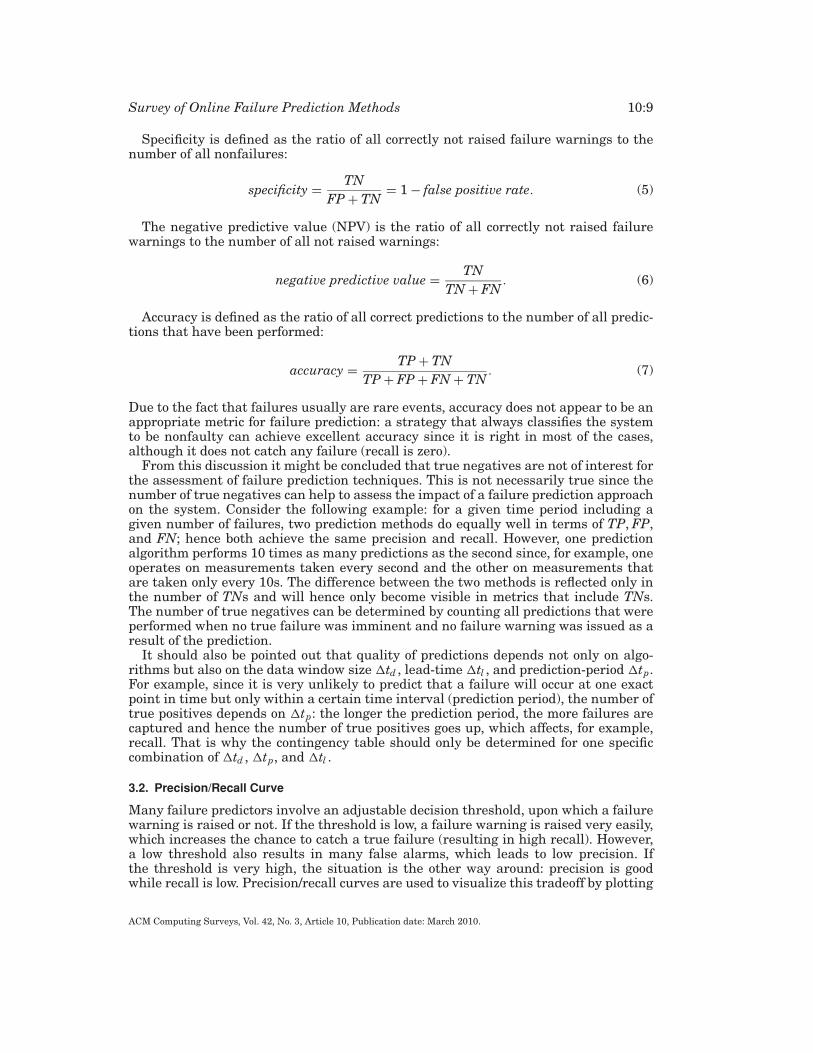
3.2. Precision/Recall Curve
Many failure predictors involve an adjustable decision threshold, upon which a failurewarning is raised or not. If the threshold is low, a failure warning is raised very easily,which increases the chance to catch a true failure (resulting in high recall). However,a low threshold also results in many false alarms, which leads to low precision. Ifthe threshold is very high, the situation is the other way around: precision is goodwhile recall is low. Precision/recall curves are used to visualize this tradeoff by plotting
ACM Computing Surveys, Vol. 42, No. 3, Article 10, Publication date: March 2010.
10:10 F. Salfner et al.
Fig. 5. Sample precision/recall curves visualizing the tradeoff between precision and recall. Curve A showsa predictor that is performing quite poorly: there is no point, where precision and recall simultaneously havehigh values. The failure prediction method pictured by curve B performs slightly better. Curve C reflects analgorithm whose predictions are mostly correct.
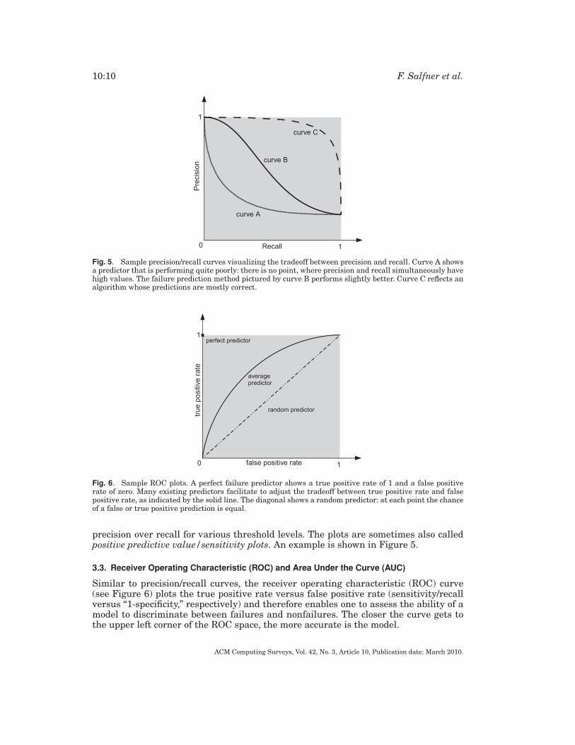
Fig. 6. Sample ROC plots. A perfect failure predictor shows a true positive rate of 1 and a false positiverate of zero. Many existing predictors facilitate to adjust the tradeoff between true positive rate and falsepositive rate, as indicated by the solid line. The diagonal shows a random predictor: at each point the chanceof a false or true positive prediction is equal.
precision over recall for various threshold levels. The plots are sometimes also calledpositive predictive value/sensitivity plots. An example is shown in Figure 5.
3.3. Receiver Operating Characteristic (ROC) and Area Under the Curve (AUC)
Similar to precision/recall curves, the receiver operating characteristic (ROC) curve(see Figure 6) plots the true positive rate versus false positive rate (sensitivity/recallversus “1-specificity,” respectively) and therefore enables one to assess the ability of amodel to discriminate between failures and nonfailures. The closer the curve gets tothe upper left corner of the ROC space, the more accurate is the model.
ACM Computing Surveys, Vol. 42, No. 3, Article 10, Publication date: March 2010.
Survey of Online Failure Prediction Methods 10:11
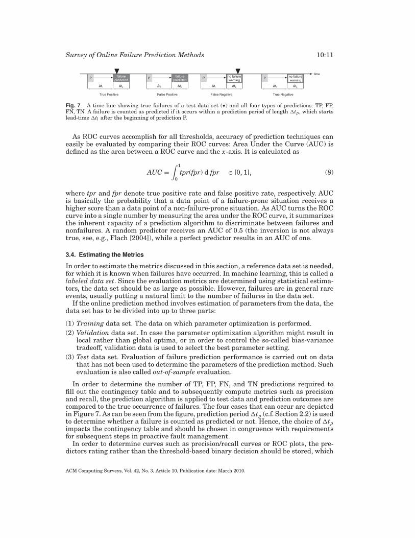
Fig. 7. A time line showing true failures of a test data set (�) and all four types of predictions: TP, FP,FN, TN. A failure is counted as predicted if it occurs within a prediction period of length �tp, which startslead-time �tl after the beginning of prediction P.
As ROC curves accomplish for all thresholds, accuracy of prediction techniques caneasily be evaluated by comparing their ROC curves: Area Under the Curve (AUC) isdefined as the area between a ROC curve and the x-axis. It is calculated as
AUC =∫ 1
0tpr(fpr) d fpr ∈ [0, 1], (8)
where tpr and fpr denote true positive rate and false positive rate, respectively. AUCis basically the probability that a data point of a failure-prone situation receives ahigher score than a data point of a non-failure-prone situation. As AUC turns the ROCcurve into a single number by measuring the area under the ROC curve, it summarizesthe inherent capacity of a prediction algorithm to discriminate between failures andnonfailures. A random predictor receives an AUC of 0.5 (the inversion is not alwaystrue, see, e.g., Flach [2004]), while a perfect predictor results in an AUC of one.
3.4. Estimating the Metrics
In order to estimate the metrics discussed in this section, a reference data set is needed,for which it is known when failures have occurred. In machine learning, this is called alabeled data set. Since the evaluation metrics are determined using statistical estima-tors, the data set should be as large as possible. However, failures are in general rareevents, usually putting a natural limit to the number of failures in the data set.
If the online prediction method involves estimation of parameters from the data, thedata set has to be divided into up to three parts:
(1) Training data set. The data on which parameter optimization is performed.(2) Validation data set. In case the parameter optimization algorithm might result in
local rather than global optima, or in order to control the so-called bias-variancetradeoff, validation data is used to select the best parameter setting.
(3) Test data set. Evaluation of failure prediction performance is carried out on datathat has not been used to determine the parameters of the prediction method. Suchevaluation is also called out-of-sample evaluation.
In order to determine the number of TP, FP, FN, and TN predictions required tofill out the contingency table and to subsequently compute metrics such as precisionand recall, the prediction algorithm is applied to test data and prediction outcomes arecompared to the true occurrence of failures. The four cases that can occur are depictedin Figure 7. As can be seen from the figure, prediction period �tp (c.f. Section 2.2) is usedto determine whether a failure is counted as predicted or not. Hence, the choice of �tpimpacts the contingency table and should be chosen in congruence with requirementsfor subsequent steps in proactive fault management.
In order to determine curves such as precision/recall curves or ROC plots, the pre-dictors rating rather than the threshold-based binary decision should be stored, which
ACM Computing Surveys, Vol. 42, No. 3, Article 10, Publication date: March 2010.
10:12 F. Salfner et al.
enables one to generate the curve for all possible threshold values using an algorithmsuch as that described in Fawcett [2004].
Estimating evaluation metrics from a finite set of test data only yields an ap-proximate assessment of the prediction performance and should hence be accompa-nied by confidence intervals. Confidence intervals are usually estimated by runningthe estimation procedure several times. Since this requires an enormous amountof data, techniques such as cross validation, jackknife, or bootstrapping are ap-plied. A more detailed discussion of such techniques can be found in Salfner [2008],Chapter 8.4.
4. A TAXONOMY OF ONLINE FAILURE PREDICTION METHODS
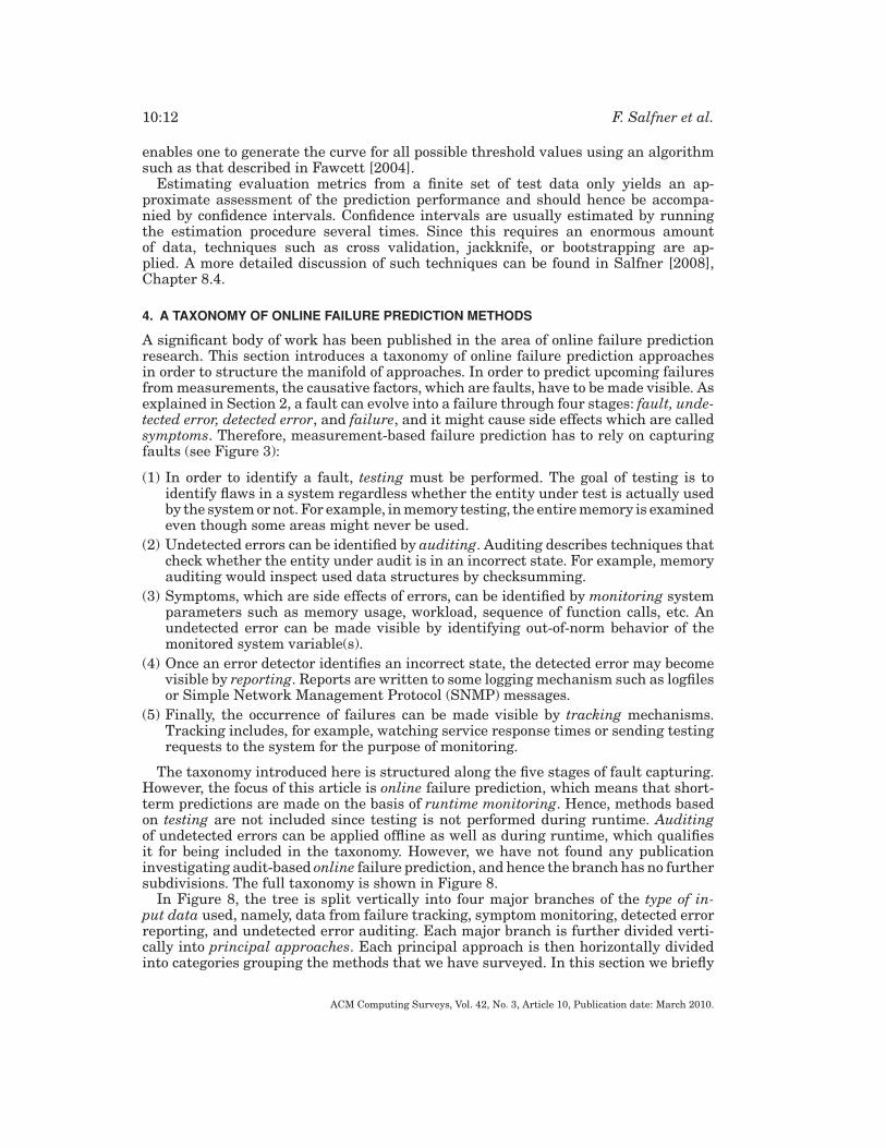
A significant body of work has been published in the area of online failure predictionresearch. This section introduces a taxonomy of online failure prediction approachesin order to structure the manifold of approaches. In order to predict upcoming failuresfrom measurements, the causative factors, which are faults, have to be made visible. Asexplained in Section 2, a fault can evolve into a failure through four stages: fault, unde-tected error, detected error, and failure, and it might cause side effects which are calledsymptoms. Therefore, measurement-based failure prediction has to rely on capturingfaults (see Figure 3):
(1) In order to identify a fault, testing must be performed. The goal of testing is toidentify flaws in a system regardless whether the entity under test is actually usedby the system or not. For example, in memory testing, the entire memory is examinedeven though some areas might never be used.
(2) Undetected errors can be identified by auditing. Auditing describes techniques thatcheck whether the entity under audit is in an incorrect state. For example, memoryauditing would inspect used data structures by checksumming.
(3) Symptoms, which are side effects of errors, can be identified by monitoring systemparameters such as memory usage, workload, sequence of function calls, etc. Anundetected error can be made visible by identifying out-of-norm behavior of themonitored system variable(s).
(4) Once an error detector identifies an incorrect state, the detected error may becomevisible by reporting. Reports are written to some logging mechanism such as logfilesor Simple Network Management Protocol (SNMP) messages.
(5) Finally, the occurrence of failures can be made visible by tracking mechanisms.Tracking includes, for example, watching service response times or sending testingrequests to the system for the purpose of monitoring.
The taxonomy introduced here is structured along the five stages of fault capturing.However, the focus of this article is online failure prediction, which means that short-term predictions are made on the basis of runtime monitoring. Hence, methods basedon testing are not included since testing is not performed during runtime. Auditingof undetected errors can be applied offline as well as during runtime, which qualifiesit for being included in the taxonomy. However, we have not found any publicationinvestigating audit-based online failure prediction, and hence the branch has no furthersubdivisions. The full taxonomy is shown in Figure 8.
In Figure 8, the tree is split vertically into four major branches of the type of in-put data used, namely, data from failure tracking, symptom monitoring, detected errorreporting, and undetected error auditing. Each major branch is further divided verti-cally into principal approaches. Each principal approach is then horizontally dividedinto categories grouping the methods that we have surveyed. In this section we briefly
ACM Computing Surveys, Vol. 42, No. 3, Article 10, Publication date: March 2010.

Survey of Online Failure Prediction Methods 10:13
Fig. 8. A taxonomy for online failure prediction approaches.
ACM Computing Surveys, Vol. 42, No. 3, Article 10, Publication date: March 2010.
10:14 F. Salfner et al.
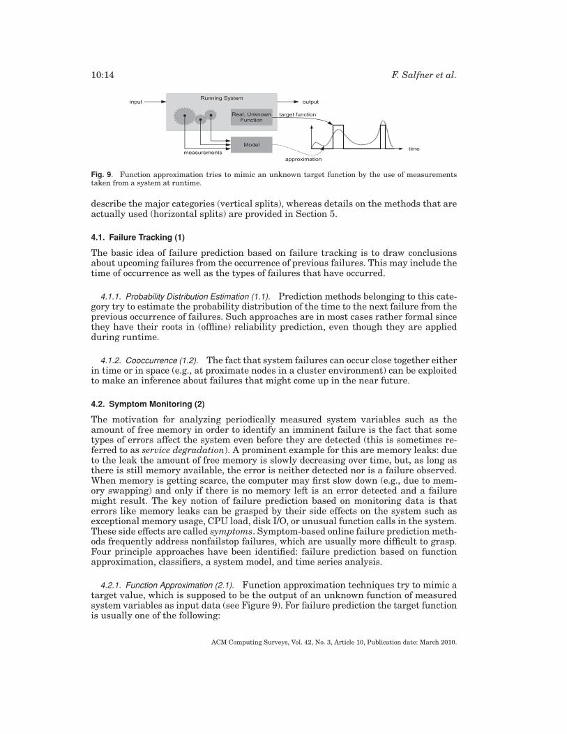
Fig. 9. Function approximation tries to mimic an unknown target function by the use of measurementstaken from a system at runtime.
describe the major categories (vertical splits), whereas details on the methods that areactually used (horizontal splits) are provided in Section 5.
4.1. Failure Tracking (1)
The basic idea of failure prediction based on failure tracking is to draw conclusionsabout upcoming failures from the occurrence of previous failures. This may include thetime of occurrence as well as the types of failures that have occurred.
4.1.1. Probability Distribution Estimation (1.1). Prediction methods belonging to this cate-gory try to estimate the probability distribution of the time to the next failure from theprevious occurrence of failures. Such approaches are in most cases rather formal sincethey have their roots in (offline) reliability prediction, even though they are appliedduring runtime.
4.1.2. Cooccurrence (1.2). The fact that system failures can occur close together eitherin time or in space (e.g., at proximate nodes in a cluster environment) can be exploitedto make an inference about failures that might come up in the near future.
4.2. Symptom Monitoring (2)
The motivation for analyzing periodically measured system variables such as theamount of free memory in order to identify an imminent failure is the fact that sometypes of errors affect the system even before they are detected (this is sometimes re-ferred to as service degradation). A prominent example for this are memory leaks: dueto the leak the amount of free memory is slowly decreasing over time, but, as long asthere is still memory available, the error is neither detected nor is a failure observed.When memory is getting scarce, the computer may first slow down (e.g., due to mem-ory swapping) and only if there is no memory left is an error detected and a failuremight result. The key notion of failure prediction based on monitoring data is thaterrors like memory leaks can be grasped by their side effects on the system such asexceptional memory usage, CPU load, disk I/O, or unusual function calls in the system.These side effects are called symptoms. Symptom-based online failure prediction meth-ods frequently address nonfailstop failures, which are usually more difficult to grasp.Four principle approaches have been identified: failure prediction based on functionapproximation, classifiers, a system model, and time series analysis.
4.2.1. Function Approximation (2.1). Function approximation techniques try to mimic atarget value, which is supposed to be the output of an unknown function of measuredsystem variables as input data (see Figure 9). For failure prediction the target functionis usually one of the following:
ACM Computing Surveys, Vol. 42, No. 3, Article 10, Publication date: March 2010.
Survey of Online Failure Prediction Methods 10:15
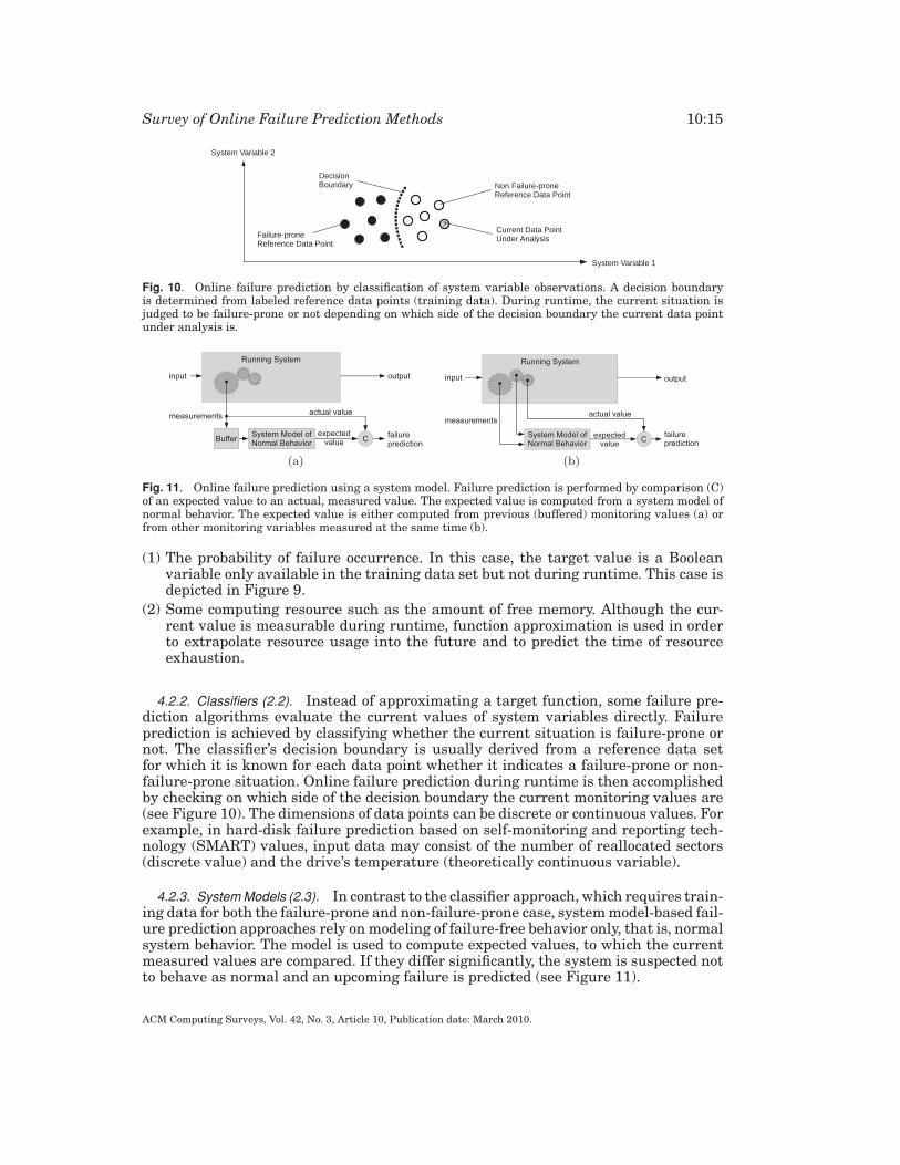
Fig. 10. Online failure prediction by classification of system variable observations. A decision boundaryis determined from labeled reference data points (training data). During runtime, the current situation isjudged to be failure-prone or not depending on which side of the decision boundary the current data pointunder analysis is.
(b)(a)
Fig. 11. Online failure prediction using a system model. Failure prediction is performed by comparison (C)of an expected value to an actual, measured value. The expected value is computed from a system model ofnormal behavior. The expected value is either computed from previous (buffered) monitoring values (a) orfrom other monitoring variables measured at the same time (b).
(1) The probability of failure occurrence. In this case, the target value is a Booleanvariable only available in the training data set but not during runtime. This case isdepicted in Figure 9.
(2) Some computing resource such as the amount of free memory. Although the cur-rent value is measurable during runtime, function approximation is used in orderto extrapolate resource usage into the future and to predict the time of resourceexhaustion.
4.2.2. Classifiers (2.2). Instead of approximating a target function, some failure pre-diction algorithms evaluate the current values of system variables directly. Failureprediction is achieved by classifying whether the current situation is failure-prone ornot. The classifier’s decision boundary is usually derived from a reference data setfor which it is known for each data point whether it indicates a failure-prone or non-failure-prone situation. Online failure prediction during runtime is then accomplishedby checking on which side of the decision boundary the current monitoring values are(see Figure 10). The dimensions of data points can be discrete or continuous values. Forexample, in hard-disk failure prediction based on self-monitoring and reporting tech-nology (SMART) values, input data may consist of the number of reallocated sectors(discrete value) and the drive’s temperature (theoretically continuous variable).
4.2.3. System Models (2.3). In contrast to the classifier approach, which requires train-ing data for both the failure-prone and non-failure-prone case, system model-based fail-ure prediction approaches rely on modeling of failure-free behavior only, that is, normalsystem behavior. The model is used to compute expected values, to which the currentmeasured values are compared. If they differ significantly, the system is suspected notto behave as normal and an upcoming failure is predicted (see Figure 11).
ACM Computing Surveys, Vol. 42, No. 3, Article 10, Publication date: March 2010.
10:16 F. Salfner et al.
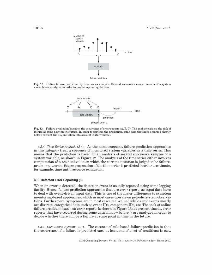
Fig. 12. Online failure prediction by time series analysis. Several successive measurements of a systemvariable are analyzed in order to predict upcoming failures.
Fig. 13. Failure prediction based on the occurrence of error reports (A, B, C). The goal is to assess the risk offailure at some point in the future. In order to perform the prediction, some data that have occurred shortlybefore present time t0 are taken into account (data window).
4.2.4. Time Series Analysis (2.4). As the name suggests, failure prediction approachesin this category treat a sequence of monitored system variables as a time series. Thismeans that the prediction is based on an analysis of several successive samples of asystem variable, as shown in Figure 12. The analysis of the time series either involvescomputation of a residual value on which the current situation is judged to be failure-prone or not, or the future progression of the time series is predicted in order to estimate,for example, time until resource exhaustion.
4.3. Detected Error Reporting (3)
When an error is detected, the detection event is usually reported using some loggingfacility. Hence, failure prediction approaches that use error reports as input data haveto deal with event-driven input data. This is one of the major differences to symptommonitoring-based approaches, which in most cases operate on periodic system observa-tions. Furthermore, symptoms are in most cases real-valued while error events mostlyare discrete, categorical data such as event IDs, component IDs, etc. The task of onlinefailure prediction based on error reports is shown in Figure 13: at present time t0, errorreports that have occurred during some data window before t0 are analyzed in order todecide whether there will be a failure at some point in time in the future.
4.3.1. Rule-Based Systems (3.1). The essence of rule-based failure prediction is thatthe occurrence of a failure is predicted once at least one of a set of conditions is met.
ACM Computing Surveys, Vol. 42, No. 3, Article 10, Publication date: March 2010.
Survey of Online Failure Prediction Methods 10:17
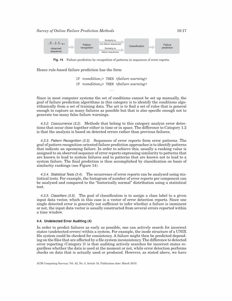
Fig. 14. Failure prediction by recognition of patterns in sequences of error reports.
Hence rule-based failure prediction has the form
IF <condition1> THEN <failure warning>IF <condition2> THEN <failure warning>
. . .
Since in most computer systems the set of conditions cannot be set up manually, thegoal of failure prediction algorithms in this category is to identify the conditions algo-rithmically from a set of training data. The art is to find a set of rules that is generalenough to capture as many failures as possible but that is also specific enough not togenerate too many false failure warnings.
4.3.2. Cooccurrence (3.2). Methods that belong to this category analyze error detec-tions that occur close together either in time or in space. The difference to Category 1.2is that the analysis is based on detected errors rather than previous failures.
4.3.3. Pattern Recognition (3.3). Sequences of error reports form error patterns. Thegoal of pattern recognition-oriented failure prediction approaches is to identify patternsthat indicate an upcoming failure. In order to achieve this, usually a ranking value isassigned to an observed sequence of error reports expressing similarity to patterns thatare known to lead to system failures and to patterns that are known not to lead to asystem failure. The final prediction is then accomplished by classification on basis ofsimilarity rankings (see Figure 14).
4.3.4. Statistical Tests (3.4). The occurrence of error reports can be analyzed using sta-tistical tests. For example, the histogram of number of error reports per component canbe analyzed and compared to the “historically normal” distribution using a statisticaltest.
4.3.5. Classifiers (3.5). The goal of classification is to assign a class label to a giveninput data vector, which in this case is a vector of error detection reports. Since onesingle detected error is generally not sufficient to infer whether a failure is imminentor not, the input data vector is usually constructed from several errors reported withina time window.
4.4. Undetected Error Auditing (4)
In order to predict failures as early as possible, one can actively search for incorrectstates (undetected errors) within a system. For example, the inode structure of a UNIXfile system could be checked for consistency. A failure might then be predicted depend-ing on the files that are affected by a file system inconsistency. The difference to detectederror reporting (Category 3) is that auditing actively searches for incorrect states re-gardless whether the data is used at the moment or not, while error detection performschecks on data that is actually used or produced. However, as stated above, we have
ACM Computing Surveys, Vol. 42, No. 3, Article 10, Publication date: March 2010.
10:18 F. Salfner et al.
not found any failure prediction approaches that apply online auditing and hence thetaxonomy contains no further subbranches.
5. SURVEY OF PREDICTION METHODS
In this survey, failure prediction methods are briefly described with appropriate refer-ence to the source, and summarized in Table III in Section 6. Representative selectedmethods are explained in greater detail in online Appendices A–K available in the ACMDigital Library.
5.1. Failure Tracking (1)
Two principal approaches to online failure prediction based on the previous occurrenceof failures can be determined: estimation of the probability distribution of a randomvariable for time to the next failure, and approaches that build on the co-occurrence offailure events.
5.1.1. Probability Distribution Estimation (1.1). In order to estimate the probability distri-bution of the time to the next failure, Bayesian predictors as well as non-parametricmethods have been applied.
5.1.1.1. Bayesian Predictors (1.1.1). The key notion of Bayesian failure prediction is toestimate the probability distribution of the next time to failure by benefiting from theknowledge obtained from previous failure occurrences in a Bayesian framework.
In Csenki [1990], such a Bayesian predictive approach [Aitchison and Dunsmore1975] was applied to the Jelinski-Moranda software reliability model [Jelinski andMoranda 1972] in order to yield an improved estimate of the next time to failure prob-ability distribution. Although developed for (offline) software reliability prediction, theapproach could be applied in an online manner as well.
5.1.1.2. Nonparametric Methods (1.1.2). It has been observed that the failure process canbe nonstationary and hence the probability distribution of time-between-failures (TBF)varies. The reasons for nonstationarity are manifold, since the fixing of bugs, changesin configuration, or even varying utilization patterns can affect the failure process. Inthese cases, techniques such as histograms result in poor estimations since station-arity (at least within a time window) is inherently assumed. For these reasons, thenonparametric method of Pfefferman and Cernuschi-Frias [2002] assumes the failureprocess to be a Bernoulli experiment where a failure of type k occurs at time n withprobability pk(n). From this assumption, it follows that the probability distribution ofTBF for failure type k is geometric since only the nth outcome is a failure of type k, andhence the probability is
Pr{
TBFk(n) = m | failure of type k at n} = pk(n)
(1 − pk(n)
)m−1. (9)
The authors proposed a method to estimate pk(n) using an autoregressive averagingfilter with a “window size” depending on the probability of the failure type k.
5.1.2. Cooccurrence (1.2). Due to sharing of resources, system failures can occur closetogether either in time or in space (at a closely coupled set of components or computers)(see, e.g., Tang and Iyer [1993]). However, in most cases, cooccurrence has been analyzedfor root cause analysis rather than failure prediction.
It has been observed several times that failures occur in clusters in a temporal as wellas in a spatial sense. Liang et al. [2006] chose such an approach to predict failures of
ACM Computing Surveys, Vol. 42, No. 3, Article 10, Publication date: March 2010.

Survey of Online Failure Prediction Methods 10:19
IBM’s BlueGene/L from event logs containing reliability, availability, and serviceabilitydata. The key to their approach is data preprocessing employing first a categorizationand then temporal and spatial compression: temporal compression combines all eventsat a single location occurring with interevent times lower than some threshold, andspatial compression combines all messages that refer to the same location within sometime window. Prediction methods are rather straightforward: using data from temporalcompression, if a failure of type application I/O or network appears, it is very likely thata next failure will follow shortly. If spatial compression suggests that some componentshave reported more events than others, it is very likely that additional failures willoccur at that location. Please refer to online Appendix B for further details.
Fu and Xu [2007] further elaborated on temporal and spatial compression and in-troduced a measure of temporal and spatial correlation of failure events in distributedsystems.
5.2. Symptom Monitoring (2)
Symptoms are side effects of errors. In this section, online failure prediction methodsare surveyed that analyze monitoring data in order to detect symptoms that indicatean upcoming failure.
5.2.1. Function Approximation (2.1). Function approximation is a term used in a largevariety of scientific areas. Applied to the task of online failure prediction, there is anassumed unknown functional relationship between monitored system variables (inputto the function) and a target value (output of the function). The objective is to revealthis relationship from measurement data.
5.2.1.1. Stochastic Models (2.1.1). Vaidyanathan and Trivedi [1999] tryed to approx-imate the amount of swap space used and the amount of real free memory (tar-get functions) from workload-related input data such as the number of system calls.They constructed a semi-Markov reward model in order to obtain a workload-basedestimation of resource consumption rate, which was then used to predict the timeto resource exhaustion. In order to determine the states of the semi-Markov rewardmodel, the input data was clustered. The authors assumed that these clusters rep-resented 11 different workload states. State transition probabilities were estimatedfrom the measurement dataset and sojourn-time distributions were obtained by fittingtwo-stage-hyperexponential or two-stage-hypoexponential distributions to the train-ing data. Then, a resource consumption “reward” rate for each workload state wasestimated from the data: Depending on the workload state the system was in, the statereward defined at what rate the modeled resource was changing. The rate was estimatedby fitting a linear function to the data using the method of Sen [1968]. Experimentshave been performed on data recorded from a SunOS 4.1.3 workstation. Please refer toonline Appendix C for more details on the approach.
Li et al. [2002] collected various parameters such as used swap space from an ApacheWeb server and built autoregressive model with auxiliary input (ARX) to predict thefurther progression of system resources utilization. Failures were predicted by estimat-ing resource exhaustion times. They compared their method to that of Castelli et al.[2001] (see Category 2.4.1) and showed that, on their data set, ARX modeling resultedin much more accurate predictions.
5.2.1.2. Regression (2.1.2). In curve fitting, which is another name for regression, pa-rameters of a function are adapted such that the curve best fits the measurement data,for example, by minimizing mean square error. The simplest form of regression is curvefitting of a linear function.
ACM Computing Surveys, Vol. 42, No. 3, Article 10, Publication date: March 2010.
10:20 F. Salfner et al.
Andrzejak and Silva [2007] applied deterministic function approximation techniquessuch as splines to characterize the functional relationships between the target function(the authors used the term aging indicator) and “work metrics” as input data. Workmetrics are, for example, the work that has been accomplished since the last restart ofthe system. Deterministic modeling offers a simple and concise description of systembehavior with few parameters. Additionally, using work-based input variables ratherthan time-based variables offers the advantage that the function does not depend onabsolute time anymore: for example, if there is only little load on a server, aging factorsaccumulate slowly and so does accomplished work whereas, in the case of high load,both accumulate more quickly. The authors presented experiments where performanceof an Apache Axis SOAP (Simple Object Access Protocol) server has been modeled asa function of various input data such as requests per second or the percentage of CPUidle time.
5.2.1.3. Machine Learning (2.1.3). Function approximation is one of the predominantapplications of machine learning. It seems natural that various techniques have along tradition in failure prediction, as can also be seen from various patents in thatarea. Troudet et al. [1990] proposed using neural networks for failure prediction ofmechanical parts and Wong et al. [1996] used neural networks to approximate theimpedance of passive components of power systems. The authors used an RLC-� model,which is a standard electronic circuit consisting of a two resistors (R), an inductor (L),and two capacities (C), where faults have been simulated to generate the trainingdata. Neville [1998] described how standard neural networks can be used for failureprediction in large-scale engineering plants.
Turning to publications regarding failure prediction in large-scale computer systems,various techniques have been applied there, too.
Hoffmann [2006] developed a failure prediction approach based on universal basisfunctions (UBF), which are an extension to radial basis functions (RBF) that use aweighted convex combination of two kernel functions instead of a single kernel. UBFapproximation has been applied to predict failures of a telecommunication system.Hoffmann et al. [2007] conducted a comparative study of several modeling techniqueswith the goal to predict resource consumption of the Apache Web server. The studyshowed that UBF turned out to yield the best results for free physical memory predic-tion, while server response times could be predicted best by support vector machines(SVM). Online Appendix D provides further details on UBF-based failure prediction.
One of the major findings in Hoffmann et al. [2007] was that the issue of choosinga good subset of input variables has a much greater influence on prediction accuracythan the choice of modeling technology. This means that the result might be better if,for example, only workload and free physical memory are taken into account and othermeasurements such as used swap space are ignored. Variable selection (some authorsalso use the term feature selection) is concerned with finding the optimal subset of mea-surements. Typical examples of variable selection algorithms are principle componentanalysis (PCA; see Hotelling [1933]) as used in Ning et al. [2006], or Forward StepwiseSelection (see, e.g., Hastie et al. [2001], Chapter 3.4.1), which was used in Turnbull andAlldrin [2003]. In addition to UBF, Hoffmann [2006] has also developed a new algo-rithm called the Probabilistic Wrapper Approach (PWA), which combines probabilistictechniques with forward selection or backward elimination.
Instance-based learning methods store the entire training dataset including inputand target values and predict by finding similar matches in the stored database oftraining data (and eventually combining them). Kapadia et al. [1999] have applied threelearning algorithms (k-nearest-neighbors, weighted average, and weighted polynomialregression) to predict the CPU time of the semiconductor manufacturing simulation
ACM Computing Surveys, Vol. 42, No. 3, Article 10, Publication date: March 2010.
Survey of Online Failure Prediction Methods 10:21
software T-Suprem3. The prediction was based on input parameters to the software suchas minimum implant energy or number of etch steps in the simulated semiconductormanufacturing process.
Fu and Xu [2007] built a neural network to approximate the number of failuresin a given time interval. The set of input variables consisted of a temporal and spatialfailure correlation factor together with variables, such as CPU utilization or the numberof packets transmitted by a computing node. The authors used (not further specified)neural networks. Data of 1 year of operation of the Wayne State University Grid wasanalyzed as a case study. Due to the fact that a correlation value of previous failures wasused as input data as well, this prediction approach also partly fits into Category 1.2.
In Abraham and Grosan [2005], the target function is the so-called stressor-susceptibility-interaction (SSI), which basically denotes failure probability as a functionof external stressors such as environment temperature or power supply voltage. Theoverall failure probability can be computed by the integration of single SSIs. The pa-per presents an approach where genetic programming has been used to generate coderepresenting the overall SSI function from training data of an electronic device’s powercircuit.
5.2.2. Classifiers (2.2). Failure prediction methods in this category build on classifiersthat are trained from failure-prone as well as non-failure-prone data samples.
5.2.2.1. Bayesian Classifiers (2.2.1). In Hamerly and Elkan [2001], two Bayesian failureprediction approaches were described. The first Bayesian classifier proposed by the au-thors is abbreviated by NBEM, expressing that a specific naıve Bayes model is trainedwith the Expectation Maximization algorithm based on a real data set of SMART val-ues of Quantum Inc. disk drives. Specifically, a mixture model was proposed whereeach naıve Bayes submodel m is weighted by a model prior P (m) and an expectationmaximization algorithm is used to iteratively adjust model priors as well as submodelprobabilities. Second, a standard naıve Bayes classifier is trained from the same inputdata set. More precisely, SMART variables xi such as read soft error rate or numberof calibration retries are divided into bins. The term naıve derives from the fact thatall attributes xi in the current observation vector �x are assumed to be independentand hence the joint probability P (�x | c) can simply be computed as the product of singleattribute probabilities P (xi | c). The authors reported that both models outperformedthe rank sum hypothesis test failure prediction algorithm of Hughes et al. [2002]5 (seeCategory 2.3.1). Please refer to online Appendix E for more details on these methods.In a later study, Murray et al. [2003], the same research group applied two additionalfailure prediction methods: support vector machines (SVM) and an unsupervised clus-tering algorithm. The SVM approach is assigned to Category 2.2.2 and the clusteringapproach belongs to Category 2.3.2.
Pizza et al. [1998] proposed a method to distinguish (i.e., classify) between transientand permanent faults: whenever erroneous component behavior is observed (e.g., bycomponent testing), the objective is to find out whether this erroneous behavior wascaused by a transient or permanent fault. Although not mentioned in the paper, thismethod could be used for failure prediction. For example, a performance failure of agrid computing application might be predicted if the number of permanent grid nodefailures exceeded a threshold (under the assumption that transient outages do notaffect overall grid performance severely). This method enables one to decide whether atested grid node has a permanent failure or not.
5Although Hughes et al. [2002] appeared after Hamerly and Elkan [2001], it was announced and submittedalready in 2000.
ACM Computing Surveys, Vol. 42, No. 3, Article 10, Publication date: March 2010.
10:22 F. Salfner et al.
5.2.2.2. Fuzzy Classifier (2.2.2). Bayes classification requires that input variables takeon discrete values. Therefore, monitoring values are frequently assigned to finite num-ber of bins (as, e.g., in Hamerly and Elkan [2001]). However, this can lead to bad assign-ments if monitoring values are close to a bin’s border. Fuzzy classification addressesthis problem by using probabilistic class membership.
Turnbull and Alldrin [2003] used radial basis functions networks (RBFNs) to classifymonitoring values of hardware sensors such as temperatures and voltages on moth-erboards. More specifically, all N monitoring values occurring within a data windowwere represented as a feature vector which was then classified as belonging to a failure-prone or non-failure-prone sequence using RBFNs. Experiments were conducted on aserver with 18 hot-swappable system boards with four processors, each. The authorsachieved good results, but failures and nonfailures were equally likely in the dataset.
Berenji et al. [2003] used an RBF rule base to classify whether a component is faultyor not: using Gaussian rules, a so-called diagnostic model computes a diagnostic signalbased on input and output values of components ranging from zero (fault-free) to 1(faulty). The rule base is algorithmically derived by means of clustering of trainingdata, which consists of input/output value pairs both for the faulty and the fault-freecase. The training data is generated from so-called component simulation models thattry to mimic the input/output behavior of system components (fault-free and faulty).The same approach is then applied on the next hierarchical level to obtain a system-wide diagnostic models. The approach has been applied to model a hybrid combustionfacility developed at the NASA Ames Research Center. The diagnostic signal can beused to predict slowly evolving failures.
Murray et al. [2003] applied SVMs in order to predict failures of hard-disk drives.SVMs were developed by Vapnik [1995] and are powerful and efficient neural networkclassifiers. In the case of hard-disk failure prediction, five successive samples of eachselected SMART attribute set up the input data vector. The training procedure of SVMsadapts the classification boundary such that the margin between the failure-prone andnon-failure-prone data points becomes maximal. Although the naıve Bayes approachdeveloped by the same group (see Hughes et al. [2002], Category 2.3.1) is mentioned inthe paper, no comparison has been carried out.
In Bodık et al. [2005] hit frequencies of Web pages were analyzed in order to quicklyidentify nonfailstop failures in the operation of a big commercial Web site. The authorsused a naıve Bayes classifier. Following the same pattern as described in Category 2.2.1,the probability P (k | �x), where k denotes the class label (normal or abnormal behavior)and �x denotes the vector of hit frequencies, was computed from likelihoods P (xi | k)which are approximated by Gaussian distributions. Since the training data set wasnot labeled (it was not known when failures had occurred), likelihoods for the failurecase were assumed to be uniformly distributed and unsupervised learning techniqueshad to be applied. The output of the naıve Bayes classifier was an anomaly score. Inthe article, a second prediction technique based on a χ2 test was proposed which isdescribed in Category 2.3.1.
Another valuable contribution of this work was a successful combination of anomalydetection and detailed analysis support in the form of a visual tool.
5.2.2.3. Other Approaches (2.2.3). In a joint effort, the University of California Berkeleyand Stanford University have developed a computing approach called recovery-orientedcomputing. As main references, see Brown and Patterson [2001] and Patterson et al.[2002] for an introduction and Candea et al. [2003, 2006] for a description of JAGR(JBoss with Application Generic Recovery), which combines several of the techniquesto build a dependable system. Although primarily targeted toward a quick detection and
ACM Computing Surveys, Vol. 42, No. 3, Article 10, Publication date: March 2010.
Survey of Online Failure Prediction Methods 10:23
analysis of failures after their occurrence, several techniques could be used for failureprediction as well. Hence, in this survey runtime path-based methods are included,which are Pinpoint (Category 2.3.1), path modeling using probabilistic context-freegrammars (Category 2.3.3), component peer models (Category 2.3.4), and decision trees,which belong to this category.
Kiciman and Fox [2005] proposed constructing a decision tree from runtime pathsin order to identify faulty components. The term runtime path denotes the sequence ofcomponents and other features such as IP addresses of server replicas in the cluster, etc.,that are involved in handling one request in a component-based software such as a J2EEapplication server. Runtime paths are obtained using Pinpoint (see Category 2.3.1).Having recorded a sufficiently large number of runtime paths including failed andsuccessful requests, a decision tree for classifying requests as failed or successful isconstructed using algorithms such as ID3 or C4.5. Although primarily designed fordiagnosis, the authors pointed out that the approach could be used for failure predictionof single requests as well.
Daidone et al. [2006] proposed using a hidden Markov model approach to inferwhether the true state of a monitored component is healthy or not. Since the outcomeof a component test does not always represent its true state, hidden Markov modelswere used where observation symbols related to outcomes of component probing, andhidden states related to the (also hidden) component’s true state. The true state (ina probabilistic sense) was inferred from a sequence of probing results by the so-calledforward algorithm of hidden Markov models. Although not intended by the authors, theapproach could be used for failure prediction in the following way: assuming that thereare some erroneous states in a system that lead to future failures and others that donot, the proposed hidden Markov model approach can be used to determine (classify)whether a failure is imminent or not on the basis of probing.
5.2.3. System Models (2.3). Online failure prediction approaches belonging to this cat-egory utilize a model of failure-free normal system behavior. The current measuredsystem behavior is compared to the expected normal behavior and a failure is pre-dicted in case of a significant deviation. We have categorized system model-based pre-diction approaches according to how normal behavior is stored: as instances, by clus-tered instances, using stochastic descriptions, or using formalisms known from controltheory.
5.2.3.1. Instance Models (2.3.1). The most straightforward data-driven way to memorizehow a system behaves normally is to store monitoring values recorded during failure-free operation. If the current monitoring values are not similar to any of the storedvalues, a failure is predicted.
Elbaum et al. [2003] carried out experiments where function calls, changes in theconfiguration, module loading, etc., of the email client “pine” had been recorded. Theauthors proposed three types of failure prediction among which sequence-based check-ing was most successful: a failure was predicted if two successive events occurringin “pine” during runtime did not belong to any of the event transitions in the storedtraining data.
Hughes et al. [2002] applied a simple albeit robust statistical test for hard-disk fail-ure prediction. The authors employed a rank sum hypothesis test to identify failureprone hard disks. The basic idea was to collect SMART values from fault-free drivesand store them as reference data set. Then, during runtime, SMART values of themonitored drive were tested the following way: the combined data set consisting ofthe reference data and the values observed at runtime was sorted and the ranks of
ACM Computing Surveys, Vol. 42, No. 3, Article 10, Publication date: March 2010.
10:24 F. Salfner et al.
the observed measurements were computed.6 The ranks were summed up and com-pared to a threshold. If the drive was not fault-free, the distribution of observed valueswere skewed and the sum of ranks tended to be greater or smaller than for fault-freedrives.
Pinpoint [Chen et al. 2002] tracked requests to a J2EE application server on theirway through the system in order to identify the software components that are correlatedwith a failure. Tracking of the requests yields a set of components used to process therequest. In case of a failure, the sets of components for several requests are clusteredusing a Jaccard score-based metric measuring similarity of the sets. A similar approachcould be applied for online failure prediction. If several sets of failure-free request pathswere stored, the same distance metric could be used to determine whether the currentset of components were similar to any of the known sets, and if not a failure would besupposed to be imminent.
In Bodık et al. [2005], which was described in Category 2.2.2, a second detec-tion/prediction technique was applied to the same data: The current hit frequenciesof the 40 most frequently used pages were compared to previous, “historically normal”hit frequencies of the same pages using a χ2 test. If the two distributions were dif-ferent with a significance level of 99%, the current observation period was declaredanomalous. In addition to this binary decision, an anomaly score was assigned to eachpage in order to support quick diagnosis. The results achieved using the χ2 test werecomparable to those of the naive Bayes approach described in Category 2.2.2.
5.2.3.2. Clustered Instance Models (2.3.2). If the amount of storage needed for instancesystem models exceeds a reasonable level or if a more general representation of traininginstances is required, training instances can be clustered. In this case, only clustercentroids or the boundaries between clusters need to be stored.
In a followup comparative study to Hughes et al. [2002] (see Category 2.3.1), Murrayet al. [2003] introduced a clustering-based failure predictor for hard-disk failure predic-tion. The basic idea was to identify areas of SMART values where a failure is very un-likely using unsupervised clustering. In other words, all areas of SMART values wherethe disk operates normally were algorithmically identified from failure-free trainingdata. In order to predict an upcoming failure, the current SMART values were as-signed to the most likely cluster. If they did not fit any known cluster (more specifically,maximum class membership probability was below a given threshold), the disk wasassumed not to behave normally and a failure was assumed to be imminent.
5.2.3.3. Stochastic Models (2.3.3). Especially in the case of complex and dynamic sys-tems, it seems appropriate to store system behavior using stochastic tools such asprobability distributions.
Ward et al. [1998] estimated the mean and variance of the number of TCP connectionsfrom two Web proxy servers in order to identify Internet service performance failures.Using a statistical test developed by Pettitt [1977], the values were compared to theprevious number of connections at the same time of the day (holidays were treatedseparately). If the current value deviated significantly, a failure was predicted.
In Chen et al. [2004]7 a runtime path analysis technique based on probabilistic con-text free grammars (PCFG) was proposed. Probabilistic context-free grammars havebeen developed in the area of statistical natural language processing (see, e.g., Manningand Schutze [1999, page 381]). The notion of the approach is to build a grammar ofall possible nonfaulty sequences of components. By assigning a probability to each
6Which in fact only involved simple counting.7The same approach was described in more detail in Kiciman and Fox [2005].
ACM Computing Surveys, Vol. 42, No. 3, Article 10, Publication date: March 2010.
Survey of Online Failure Prediction Methods 10:25
grammar rule, the overall probability of a given sequence of components can be com-puted. From this, an anomaly score is computed and, if a sufficiently large amount ofpaths (i.e., requests) have a high anomaly score, a failure is assumed. The approachhas been applied to call paths collected from a Java 2 Enterprise Edition (J2EE) demoapplication, an industrial enterprise voice application network, and from eBay servers.Although not intended by the authors, the same approach could be used to predict, forexample, service level failures: if a significant amount of requests do not seem to behavenormally, the system might not be able to deliver the required level of service shortly inthe future. It might also be applicable for request failure prediction: if the probabilityof the beginning of a path is very low, there is an increased probability that a failurewill occur in the further course of the request.
5.2.3.4. Graph Models (2.3.4). In Kiciman and Fox [2005], a second approach was pro-posed based on component interaction graphs (a so-called peer model). The peer modelreflects how often one component interacts with another component: each componentis a node and how often one component interacts with another is expressed by weightedlinks. One specific instance of a component is checked to see whether it is errorfree byusing a χ2 goodness-of-fit test: if the proportion of runtime paths between a componentinstance and other component classes deviates significantly from the reference modelrepresenting fault-free behavior, the instance is suspected to be faulty. By conducting atrend analysis on the anomaly score, a future failure of the component instance mightbe predicted.
5.2.3.5. Control Theory Models (2.3.5). It is common in control theory to have an abstrac-tion of the controlled system estimating the internal state of the system and its progres-sion over time by some mathematical equations, such as linear equation systems, differ-ential equation systems, Kalman filters, etc. (see, e.g., Lunze [2003], Chapter 4). Thesemethods are widely used for fault diagnosis (see, e.g., Korbicz et al. [2004], Chapters 2and 3) but have only rarely been used for failure prediction. However, many of themethods inherently include the possibility of predicting future behavior of the systemand hence have the ability to predict failures. For example, in his doctoral dissertationNeville [1998] described the prediction of failures in large-scale engineering plants.Another example was Discenzo et al. [1999], who mention that such methods havebeen used to predict failures of an intelligent motor using the standard IEEE motormodel.
With regard to online failure prediction, Singer et al. [1997] proposed the MultivariateState Estimation Technique (MSET) to detect system disturbances by a comparisonof the estimated and measured system state. More precisely, a matrix D of selectedmeasurement data of normal operation is collected. In the operational phase, a stateestimation is computed as a combination of D and the current (runtime) observations.The difference between the observed and estimated states constitutes a residual thatis checked for significant deviation by a sequential probability ratio test (SPRT). Grosset al. [2002] applied the method to detect software aging [Parnas 1994] in an experimentwhere a memory-leak fault injector consumed system memory at an adjustable rate.MSET and SPRT have been used to detect whether the fault injector was active and, ifso, at what rate it was operating. By this, time to memory consumption can be estimated.MSET has also been applied to online transaction processing servers in order to detectsoftware aging [Cassidy et al. 2002].
5.2.3.6. Other Potential Approaches. A more theoretic approach that could in principlebe applied to online failure prediction is to abstract system behavior by a queuing modelthat incorporates additional knowledge about the current state of the system. Failureprediction can be performed by computing the input value dependent expected response
ACM Computing Surveys, Vol. 42, No. 3, Article 10, Publication date: March 2010.
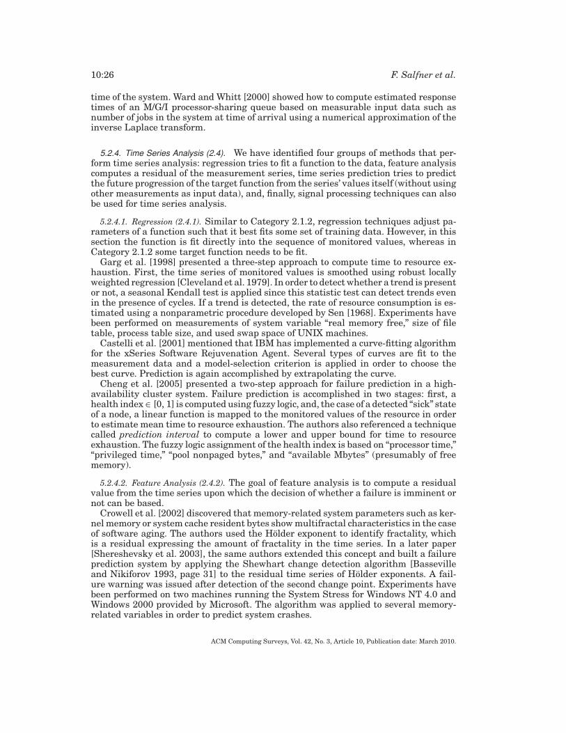
10:26 F. Salfner et al.
time of the system. Ward and Whitt [2000] showed how to compute estimated responsetimes of an M/G/I processor-sharing queue based on measurable input data such asnumber of jobs in the system at time of arrival using a numerical approximation of theinverse Laplace transform.
5.2.4. Time Series Analysis (2.4). We have identified four groups of methods that per-form time series analysis: regression tries to fit a function to the data, feature analysiscomputes a residual of the measurement series, time series prediction tries to predictthe future progression of the target function from the series’ values itself (without usingother measurements as input data), and, finally, signal processing techniques can alsobe used for time series analysis.
5.2.4.1. Regression (2.4.1). Similar to Category 2.1.2, regression techniques adjust pa-rameters of a function such that it best fits some set of training data. However, in thissection the function is fit directly into the sequence of monitored values, whereas inCategory 2.1.2 some target function needs to be fit.
Garg et al. [1998] presented a three-step approach to compute time to resource ex-haustion. First, the time series of monitored values is smoothed using robust locallyweighted regression [Cleveland et al. 1979]. In order to detect whether a trend is presentor not, a seasonal Kendall test is applied since this statistic test can detect trends evenin the presence of cycles. If a trend is detected, the rate of resource consumption is es-timated using a nonparametric procedure developed by Sen [1968]. Experiments havebeen performed on measurements of system variable “real memory free,” size of filetable, process table size, and used swap space of UNIX machines.
Castelli et al. [2001] mentioned that IBM has implemented a curve-fitting algorithmfor the xSeries Software Rejuvenation Agent. Several types of curves are fit to themeasurement data and a model-selection criterion is applied in order to choose thebest curve. Prediction is again accomplished by extrapolating the curve.
Cheng et al. [2005] presented a two-step approach for failure prediction in a high-availability cluster system. Failure prediction is accomplished in two stages: first, ahealth index ∈ [0, 1] is computed using fuzzy logic, and, the case of a detected “sick” stateof a node, a linear function is mapped to the monitored values of the resource in orderto estimate mean time to resource exhaustion. The authors also referenced a techniquecalled prediction interval to compute a lower and upper bound for time to resourceexhaustion. The fuzzy logic assignment of the health index is based on “processor time,”“privileged time,” “pool nonpaged bytes,” and “available Mbytes” (presumably of freememory).
5.2.4.2. Feature Analysis (2.4.2). The goal of feature analysis is to compute a residualvalue from the time series upon which the decision of whether a failure is imminent ornot can be based.
Crowell et al. [2002] discovered that memory-related system parameters such as ker-nel memory or system cache resident bytes show multifractal characteristics in the caseof software aging. The authors used the Holder exponent to identify fractality, whichis a residual expressing the amount of fractality in the time series. In a later paper[Shereshevsky et al. 2003], the same authors extended this concept and built a failureprediction system by applying the Shewhart change detection algorithm [Bassevilleand Nikiforov 1993, page 31] to the residual time series of Holder exponents. A fail-ure warning was issued after detection of the second change point. Experiments havebeen performed on two machines running the System Stress for Windows NT 4.0 andWindows 2000 provided by Microsoft. The algorithm was applied to several memory-related variables in order to predict system crashes.
ACM Computing Surveys, Vol. 42, No. 3, Article 10, Publication date: March 2010.
Survey of Online Failure Prediction Methods 10:27
Fig. 15. Failure prediction using signal processing techniques on measurement data.
5.2.4.3. Time Series Prediction (2.4.3). Hellerstein et al. [1999], described an approachto predict if a time series will violate a threshold. In order to achieve this, several timeseries models are employed to model stationary as well as nonstationary effects. Forexample, the model accounts for the influence of the day-of-the-week, or time-of-the-day,etc. Experiments have been carried out on prediction of HTTP operations per secondof a production Web server. A similar approach has also been described in Vilalta et al.[2002]. In online Appendix F, a more detailed description of this method can be found.
Sahoo et al. [2003] applied various time series models to data of a 350-node clus-ter system to predict parameters like percentage of system utilization, idle time, andnetwork IO.
A relatively new technique on the rise is based on “rough set theory” [Pawlak et al.1988], which is an approximation of conventional sets by providing a set of upper andlower values. Meng et al. [2007] combined rough set theory with wavelet networks inorder to predict memory usage of a J2EE application server. In the experiments, memoryusage was monitored every 12 min and the next monitoring value was predicted basedon a series of previous monitoring values. From this one-step-ahead prediction of themonitoring variable, it follows that the lead time �tl equals the monitoring period(12 min in this case). The same authors published a similar paper about a combinationof fuzzy logic and wavelet networks [Ning et al. 2006], which are called fuzzy waveletnetworks (FWN) [Ho et al. 2001].
5.2.4.4. Other Potential Approaches. Signal processing techniques are of course relatedto methods that have already been described (e.g., Kalman filters in Category 2.3.5).Algorithms that fall into this category use signal processing techniques such as low-pass or noise filtering to obtain a clean estimate of a system resource measurement.For example, if free system memory is measured, observations will vary greatly due tothe allocation and freeing of memory. Such measurement series can be seen as a noisysignal where noise filtering techniques can be applied in order to obtain the “true”behavior of free system memory: if it is a continuously decreasing function, softwareaging is likely in progress and the amount of free memory can be estimated for the nearfuture by means of signal processing prediction methods such as low-pass filtering orfrequency transformation (see Figure 15).
5.3. Detected Error Reporting (3)
There are two main groups of failure prediction approaches that analyze error reports:rule-based or error pattern-based approaches.
5.3.1. Rule-Based Approaches (3.1). Failure prediction methods in this category derivea set of rules where each rule consists of error reports.
To our knowledge, the first rule-based approach to failure prediction based on re-ported error events was published by Hatonen et al. [1996]. The authors described asystem that identifies episode rules from error logs (the authors used the term alarm).Episode rules express temporal ordering of events in the form “if errors A and B oc-cur within five seconds, then error C occurs within 30 s with probability 0.8.” Several
ACM Computing Surveys, Vol. 42, No. 3, Article 10, Publication date: March 2010.
10:28 F. Salfner et al.
parameters such as the maximum length of the data window, types of error messages,and ordering requirements have to be prespecified. However, the algorithm returnedtoo many rules such that they had to be presented to human operators with systemknowledge in order to filter out informative ones.
Weiss [1999] introduced a failure prediction technique called timeweaver that basedon a genetic training algorithm. In contrast to searching and selecting patterns thatexist in the database, rules are generated “from scratch” by the use of a simple lan-guage: error events are connected with three types of ordering primitives. The geneticalgorithm starts with an initial set of rules (initial population) and repetitively appliescrossing and mutation operations to generate new rules. The quality of the obtainedcandidates is assessed using a special fitness function that incorporates both predic-tion quality (based on a variant of the F-measure, that allows one to adjust the relativeweight of precision and recall) and diversity of the rule set. After generating a ruleset with the genetic algorithm, the rule set is pruned in order to remove redundantpatterns. The approach was applied to telecommunication equipment failure data andresults compared to three standard machine learning algorithms: C4.5rules [Quinlan1993], RIPPER [Cohen 1995], and FOIL [Quinlan 1990]. Please refer to online AppendixG for further details on timeweaver.
Vilalta and Ma [2002] described a data-mining approach that is tailored to short-termprediction of Boolean data building on a concept termed eventsets. The method searchesfor predictive subsets of events occurring prior to a target event. In the terminology usedhere, events refer to error reports and target events to failures. The method addressesthe issue of class skewness (failures occur very rarely in comparison to nonfailureevents) by first considering only failure-prone sequences, and by incorporating non-failure-prone data in a later step. More precisely, the method is divided into three steps:first, frequent subsets of error events preceding a failure are extracted. Second, subsetsthat occur frequently before failures but also frequently when no failure occurs areremoved by a threshold on confidence and by applying a statistical test. In a final thirdstep, overly general sets are removed. Please refer to online Appendix H for furtherdetails on this approach. The eventset method has been applied to failure prediction ina 350-node cluster system, as described in Sahoo et al. [2003] (Category 2.4.3).
5.3.1.1. Other Potential Approaches. Fault trees were developed in the 1960s and havebecome a standard tool reliability modeling. A comprehensive treatment of fault treeswas given, for example, by Vesely et al. [1981]. The purpose of fault trees is to modelconditions under which failures can occur using logical expressions. Expressions arearranged in the form of a tree, and probabilities are assigned to the leaf nodes, facili-tating the computation of the overall failure probability. Fault tree analysis is a staticalanalysis that does not take the current system status into account. However, if the leafnodes are combined with online fault detectors, and logical expressions are transformedinto a set of rules, they can be used as a rule-based online failure predictor. Althoughsuch an approach has been applied to chemical process failure prediction [Ulerich andPowers 1988] and power systems [Rovnyak et al. 1994], we have not found the approachbeing applied to computer systems.
Bai et al. [2005] employed a Markov Bayesian Network for reliability prediction buta similar approach might work for online failure prediction as well. The same holds fordecision tree methods: upcoming failures can be predicted if error events are classifiedusing a decision tree approach similar to that proposed by Kiciman and Fox [2005] (seeCategory 2.2.3). In this case, however, the decision tree would have to classify errorreports rather than monitored runtime paths.
Regarding data mining, several developments could potentially be used to furtherimprove data mining-based online failure prediction: sequential pattern mining and
ACM Computing Surveys, Vol. 42, No. 3, Article 10, Publication date: March 2010.
Survey of Online Failure Prediction Methods 10:29
the use of ontologies, as described in, for example, Srikant and Agrawal [1996], or pathtraversal patterns (see, e.g., Chen et al. [1998]), which could be applied in transaction-based systems.
5.3.2. Cooccurrence (3.2). Levy and Chillarege [2003] analyzed data of an industrialvoice mail system and identified three characteristics they called principles, two ofwhich support the assumptions on which failure prediction approaches in this categoryare based: principle 1 (“counts tell”) again emphasizes the property that the numberof errors (since the article is about a telecommunication system, the authors used theterm alarm for what is termed an error, here) per time unit increases before a failure.Principle 2 (“the mix changes”) is described in Category 3.4. Principle 3 (“clusters formearly”) basically is the same as principle 1 but puts more emphasis on the fact that forcommon failures the effect is even more apparent if errors are clustered into groups.Similar observations have been made by Liang et al. [2006]: the authors analyzed jobsof an IBM BlueGene/L supercomputer and supported the following thesis: “On average,we observe that if a job experiences two or more nonfatal events after filtering, thenthere is a 21.33% chance that a fatal failure will follow. For jobs that only have onenonfatal event, this probability drops to 4.7%” (p. 444).
According to Siewiorek and Swarz [1998], page 262, Nassar and Andrews [1985]were one of the first to propose two ways of failure prediction based on the occurrenceof error reports. The first approach investigates the distribution of error types. If thedistribution of error types changes systematically (i.e., one type of error occurs morefrequently), a failure is supposed to be imminent. The second approach investigateserror distributions for all error types obtained for intervals between crashes. If the errorgeneration rate increases significantly, a failure is looming. Both approaches result inthe computation of threshold values upon which a failure warning can be issued.
The dispersion frame technique (DFT) developed by Lin and Siewiorek [1990] usesa set of heuristic rules on the time of occurrence of consecutive error events of eachcomponent to identify looming permanent failures. A detailed description of the DFTcan be found in online Appendix I.
Lal and Choi [1998] showed plots and histograms of errors occurring in a UNIXServer. The authors proposed aggregating errors in an approach similar to tupling (c.f.Tsao and Siewiorek [1983]) and stated that the frequency of clustered error occurrenceindicates an upcoming failure. Furthermore, they showed histograms of error occur-rence frequency over time before failure.
More recently, Leangsuksun et al. [2004] presented a study where hardware sen-sors measurements such as fan speed, temperature, etc., are aggregated using severalthresholds to generate error events with several levels of criticality. These events are an-alyzed in order to eventually generate a failure warning that can be processed by othermodules. The study was carried out on data of a high-availability, high-performanceLinux cluster.
5.3.3. Pattern Recognition (3.3). Pattern recognition techniques operate on sequencesof error events trying to identify patterns that indicate a failure-prone system state.
Methods such as eventset [Vilalta et al. 2002] investigate the type of error reports(e.g., the error message ID) while methods such as the dispersion frame technique[Lin and Siewiorek 1990] focus on the time when errors are detected. If both parts oferror reports—time and type—are considered together, the sequence of error reportsturns into a temporal sequence. Salfner and colleagues proposed two failure predictionmethods that identify patterns in temporal sequences.
Salfner et al. [2006] presented Similar Events Prediction (SEP), which is a semi-Markov chain model. Each error report event corresponds to a state in the semi-Markov
ACM Computing Surveys, Vol. 42, No. 3, Article 10, Publication date: March 2010.
10:30 F. Salfner et al.
chain while the time between two reports is represented by the continuous-time statetransition duration of the semi-Markov chain using uniform distributions. Sequencesimilarity is computed by the product of state traversal probabilities. Training of themodel involves hierarchical clustering of error sequences leading to a failure and thecomputation of relative frequencies to estimate state transition probabilities. The arti-cle included experiments with data from an industrial telecommunication system.
Salfner and Malek [2007] proposed using hidden semi-Markov models (HSMM) inorder to add one additional level of flexibility. Associating error detections with obser-vations that are generated by the states of the HSMM, errors may be mapped to groupsof hidden states. With HSMMs, similarity of error sequences can be computed by theuse of the forward algorithm, which is an efficient dynamic programming algorithm tocompute the sequence likelihood. One advantage of HSMMs in comparison to Salfneret al. [2006] is that HSMMs can handle permutations in the input event sequences.In addition to the classification step depicted in Figure 14, which is an evaluation offailure probability for some fixed point in time in the future, failure prediction canalso be accomplished by computing the time-to-failure distribution (c.f. Salfner [2006]).Salfner [2008] provided more details on the HSMM method, including a comparativeanalysis of HSMM with DFT, eventset method, and SVD-SVM (see Category 3.5). Thestudy also included a comparison of computational overhead both for the training andapplication of the methods.
5.3.3.1. Other Potential Approaches. Computing the similarity between sequences is oneof the key tasks in biological sequence analysis [Durbin et al. 1998, Chapter 2], whichis called pairwise alignment. Various algorithms have been developed such as theNeedleman-Wunsch algorithm [Needleman and Wunsch 1970] the Smith-Watermanalgorithm [Smith and Waterman 1981], or the BLAST algorithm [Altschul et al. 1990].The outcome of such algorithms is usually a score evaluating the alignment of twosequences. If used as a similarity measure between the sequence under investigationand known failure sequences, failure prediction can be accomplished as depicted inFigure 14. One of the advantages of alignment algorithms is that they build on a sub-stitution matrix providing scores for the substitution of symbols. In terms of error eventsequences, this technique has the potential to define a score for one error event being“replaced” by another event, giving rise to the use of a hierarchical grouping of errors,as proposed in Salfner et al. [2004].
In Category 2.3.3, the method of Kiciman and Fox [2005] was described, which usedprobabilistic context-free grammars (PCFG) to analyze runtime paths. However, run-time paths contain symptoms rather than errors. Nevertheless, PCFGs could also beused to perform error report-based failure prediction: following the approach depictedin Figure 14, PCFGs can be used to compute sequence similarity to error report se-quences that have lead to a failure in the training dataset, and to compute sequencesimilarity to error report sequences that usually do not lead to a failure.
A further well-known stochastic speech modeling technique is n-gram models[Manning and Schutze 1999, page 192]. n-grams represent sentences by conditionalprobabilities taking into account a context of up to n words in order to compute theprobability of a given sentence.8 Conditional densities are estimated from training data.Transferring this concept to failure prediction, error events correspond to words anderror sequences to sentences. If the probabilities (the “grammar”) of an n-gram modelwere estimated from failure sequences, high sequence probabilities would translateinto “failure-prone” and low probabilities into “not failure-prone”.
8Although, in most applications of statistical natural language processing, the goal is to predict the nextword using P (wn|w1, . . . , wn−1), the two problems are connected via the theorem of conditional probabilities.
ACM Computing Surveys, Vol. 42, No. 3, Article 10, Publication date: March 2010.
Survey of Online Failure Prediction Methods 10:31
5.4. Statistical Tests (3.4)
Principle 2 (“the mix changes”) in Levy and Chillarege [2003] mentioned in Cate-gory 3.2 delineates the discovery that the order of subsystems sorted by error generationfrequency changes prior to a failure. According to the article, relative error generationfrequencies of subsystems follow a Pareto distribution: most errors are generated byonly a few subsystems while most subsystems generate only very few errors (which isalso known as Zipf’s law [Zipf 1949]). The proposed failure prediction algorithm mon-itors the order of subsystems and predicts a failure if it changes significantly, whichbasically is a statistical test. Using data of the voice mail application analyzed, the au-thors showed examples where the change in order can be observed; however, no resultswith respect to false negatives or false positives were reported.
5.5. Classifiers (3.5)
Classifiers usually associate an input vector with a class label. In this Category 3, inputdata consists of one or more error reports that have to be represented by a vector inorder to be processed by a classification algorithm. A straightforward solution would beto use the error type of the first event in a sequence as the value of the first input vectorcomponent, the second type as the second component, and so on. However, it turnsout that such a solution does not the work: if the sequence is shifted only one step,the sequence vector is orthogonally rotated in the input space and most classifiers willnot judge the two vectors as similar. One solution to this problem has been proposedby Domeniconi et al. [2002]: SVD-SVM (Singular-Value-Decomposition and Support-Vector-Machine) borrows a technique known from information retrieval: the so-called“vector space model” representation of texts [Manning and Schutze 1999, page 539].In the vector space model representation, there is a dimension for each word of thelanguage. Each text is a point in this high-dimensional space where the magnitudealong each dimension is defined by the number of occurrences of the specific word in thetext. SVD-SVM applies the same technique to represent error event sequences: Eachdimension of the vector corresponds to one event type and the magnitude is eithera Boolean value indicating whether an error type is present or not, the number ofoccurrences of the event type in the data window, or a binary encoded timestamp. SVD-SVM performs two steps: the first step involves the simplification and decorrelation ofevent sequences by the use of singular value decomposition. The second step involvesclassification by the use of support vector machines. The approach has been applied todata of a production computer network where failures were defined to be the occurrenceof an error event with severity level “critical” or “fatal.” Further details on this methodcan be found in online Appendix K.
6. SUMMARY AND CONCLUSIONS
We have surveyed failure prediction methods that have been proposed and many ofthem used to predict failures of computer systems online. The goal of online failureprediction is to identify if a failure, which is a misbehavior of the system resultingin a deviation from the expected output, will occur in the near future. This can beaccomplished by runtime observation and measurement of the current system state.Although failure prediction approaches exist that base predictions on upcoming failureswithout measuring the current system state (e.g., by lifetime probability distributions),these are beyond the scope of this survey.
We have developed a comprehensive taxonomy in order to structure and classify awide spectrum of existing techniques dealing with online failure prediction to helppotential users to easily find a method that might be attractive in their application
ACM Computing Surveys, Vol. 42, No. 3, Article 10, Publication date: March 2010.
10:32 F. Salfner et al.
environment. Online failure prediction methods can be divided into four categories ac-cording to the type of input data that is processed. Specifically, the approaches evaluate(a) the times of previous failure occurrence (failure tracking), (b) monitoring data re-flecting symptoms (side effects) of errors, (c) the detection of errors that have not yetevolved to become a failure, or (d) the search for undetected errors by means of auditing.Three of the categories have been divided further by the principle approach they em-ploy and subsequently by the methods they use. Concepts have been briefly explained,followed by appropriate references.
We have surveyed almost 50 approaches from various research areas such as pat-tern recognition, control theory, and function approximation. The majority of describedapproaches focus on failure prediction concerning software but there are also manymethods predicting failures of hardware, for example, Hughes et al. [2002], Hamerlyand Elkan [2001], Murray et al. [2003], or Weiss [1999].
A comprehensive summary of all models/approaches together with demonstrated ap-plications including appropriate references and classification can be found in Table III.In addition, the table provides a brief synopsis of each approach and its potential appli-cation areas, along with remarks about it. In order to shorten the table, the followingnumbers are used for text that appears several times across the table:
Failure-based long term prediction;Failure prediction in distributed systems;Prediction of resource-scarcity failures;Prediction of service level failures;Single request failure prediction;Component failure prediction;Event-based failure prediction (as a superset to error reports).
In order to provide better insight into categories, the online appendices describe var-ious approaches that are representative for each category. Table IV online Appendix Alists the approaches that are described in online Appendices B to K. Classificationrefers to the category of our taxonomy the approach is assigned to; application areadenotes the areas the method was or could be implemented in, the metrics indicatesused to assess the quality of the corresponding failure prediction approach;’ and, finally,failure model names the failures and/or faults that can be predicted by the examinedtechnique. Most of these techniques have been tested and evaluated in practice.
Let us reiterate and summarize: dependability and resilience are and will remain apermanent challenge for the following reasons:
—ever-increasing systems complexity,—ever-growing number of attacks and threats,—novice users,—third-party, open-source software, commercial-off-the-shelf (COTS) components,—growing connectivity and interoperability,—dynamicity (frequent configurations, reconfigurations, updates, upgrades and
patches, ad hoc extensions), and—systems proliferation to applications in all domains of human activity.
In such circumstances, proactive fault management by runtime monitoring and on-line failure prediction seem to be one of a very few alternatives for effective online de-pendability assessment and enhancement. In our opinion, proactive fault management
ACM Computing Surveys, Vol. 42, No. 3, Article 10, Publication date: March 2010.
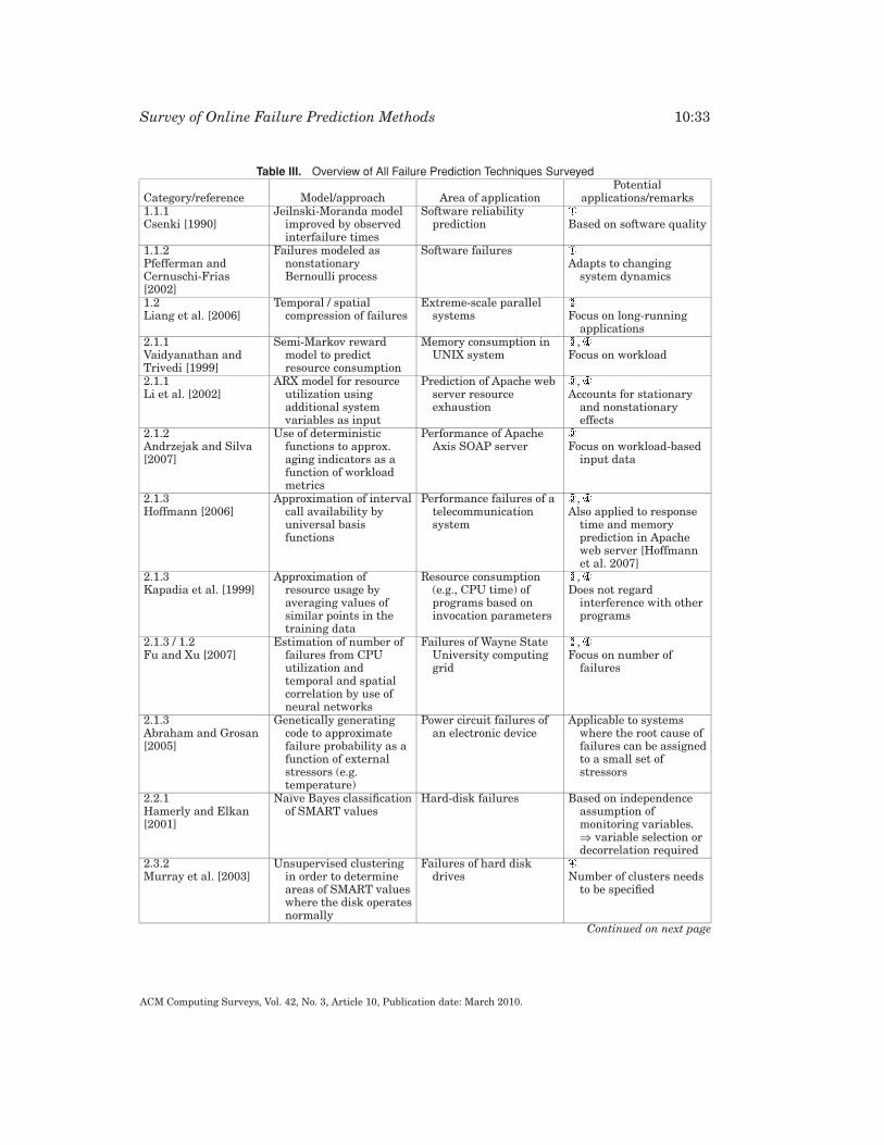
Survey of Online Failure Prediction Methods 10:33
Table III. Overview of All Failure Prediction Techniques SurveyedPotential
Category/reference Model/approach Area of application applications/remarks1.1.1Csenki [1990]
Jeilnski-Moranda modelimproved by observedinterfailure times
Software reliabilityprediction Based on software quality
1.1.2Pfefferman andCernuschi-Frias[2002]
Failures modeled asnonstationaryBernoulli process
Software failuresAdapts to changing
system dynamics
1.2Liang et al. [2006]
Temporal / spatialcompression of failures
Extreme-scale parallelsystems Focus on long-running
applications2.1.1Vaidyanathan andTrivedi [1999]
Semi-Markov rewardmodel to predictresource consumption
Memory consumption inUNIX system
,Focus on workload
2.1.1Li et al. [2002]
ARX model for resourceutilization usingadditional systemvariables as input
Prediction of Apache webserver resourceexhaustion
,Accounts for stationary
and nonstationaryeffects
2.1.2Andrzejak and Silva[2007]
Use of deterministicfunctions to approx.aging indicators as afunction of workloadmetrics
Performance of ApacheAxis SOAP server Focus on workload-based
input data
2.1.3Hoffmann [2006]
Approximation of intervalcall availability byuniversal basisfunctions
Performance failures of atelecommunicationsystem
,Also applied to response
time and memoryprediction in Apacheweb server [Hoffmannet al. 2007]
2.1.3Kapadia et al. [1999]
Approximation ofresource usage byaveraging values ofsimilar points in thetraining data
Resource consumption(e.g., CPU time) ofprograms based oninvocation parameters
,Does not regard
interference with otherprograms
2.1.3 / 1.2Fu and Xu [2007]
Estimation of number offailures from CPUutilization andtemporal and spatialcorrelation by use ofneural networks
Failures of Wayne StateUniversity computinggrid
,Focus on number of
failures
2.1.3Abraham and Grosan[2005]
Genetically generatingcode to approximatefailure probability as afunction of externalstressors (e.g.temperature)
Power circuit failures ofan electronic device
Applicable to systemswhere the root cause offailures can be assignedto a small set ofstressors
2.2.1Hamerly and Elkan[2001]
Naıve Bayes classificationof SMART values
Hard-disk failures Based on independenceassumption ofmonitoring variables.⇒ variable selection ordecorrelation required
2.3.2Murray et al. [2003]
Unsupervised clusteringin order to determineareas of SMART valueswhere the disk operatesnormally
Failures of hard diskdrives Number of clusters needs
to be specified
Continued on next page
ACM Computing Surveys, Vol. 42, No. 3, Article 10, Publication date: March 2010.
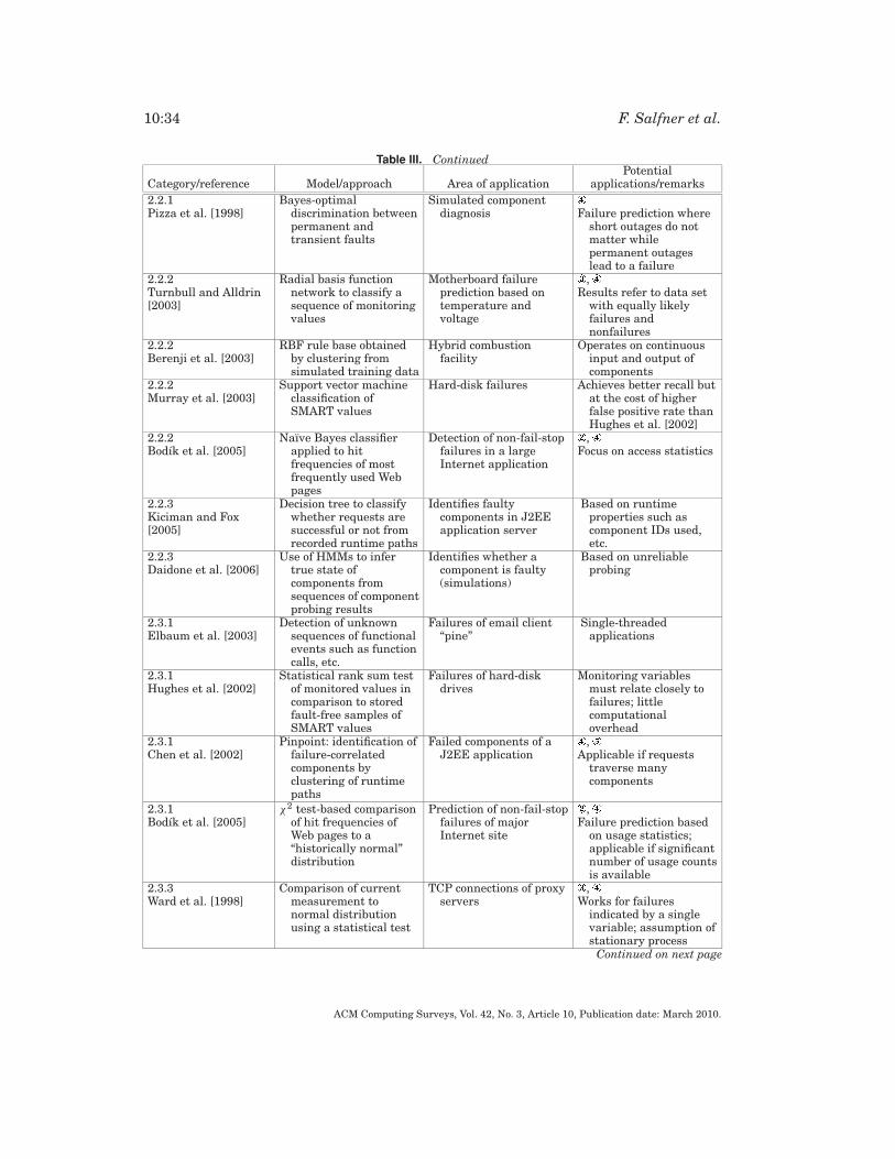
10:34 F. Salfner et al.
Table III. ContinuedPotential
Category/reference Model/approach Area of application applications/remarks2.2.1Pizza et al. [1998]
Bayes-optimaldiscrimination betweenpermanent andtransient faults
Simulated componentdiagnosis Failure prediction where
short outages do notmatter whilepermanent outageslead to a failure
2.2.2Turnbull and Alldrin[2003]
Radial basis functionnetwork to classify asequence of monitoringvalues
Motherboard failureprediction based ontemperature andvoltage
,Results refer to data set
with equally likelyfailures andnonfailures
2.2.2Berenji et al. [2003]
RBF rule base obtainedby clustering fromsimulated training data
Hybrid combustionfacility
Operates on continuousinput and output ofcomponents
2.2.2Murray et al. [2003]
Support vector machineclassification ofSMART values
Hard-disk failures Achieves better recall butat the cost of higherfalse positive rate thanHughes et al. [2002]
2.2.2Bodık et al. [2005]
Naıve Bayes classifierapplied to hitfrequencies of mostfrequently used Webpages
Detection of non-fail-stopfailures in a largeInternet application
,Focus on access statistics
2.2.3Kiciman and Fox[2005]
Decision tree to classifywhether requests aresuccessful or not fromrecorded runtime paths
Identifies faultycomponents in J2EEapplication server
Based on runtimeproperties such ascomponent IDs used,etc.
2.2.3Daidone et al. [2006]
Use of HMMs to infertrue state ofcomponents fromsequences of componentprobing results
Identifies whether acomponent is faulty(simulations)
Based on unreliableprobing
2.3.1Elbaum et al. [2003]
Detection of unknownsequences of functionalevents such as functioncalls, etc.
Failures of email client“pine”
Single-threadedapplications
2.3.1Hughes et al. [2002]
Statistical rank sum testof monitored values incomparison to storedfault-free samples ofSMART values
Failures of hard-diskdrives
Monitoring variablesmust relate closely tofailures; littlecomputationaloverhead
2.3.1Chen et al. [2002]
Pinpoint: identification offailure-correlatedcomponents byclustering of runtimepaths
Failed components of aJ2EE application
,Applicable if requests
traverse manycomponents
2.3.1Bodık et al. [2005]
χ2 test-based comparisonof hit frequencies ofWeb pages to a“historically normal”distribution
Prediction of non-fail-stopfailures of majorInternet site
,Failure prediction based
on usage statistics;applicable if significantnumber of usage countsis available
2.3.3Ward et al. [1998]
Comparison of currentmeasurement tonormal distributionusing a statistical test
TCP connections of proxyservers
,Works for failures
indicated by a singlevariable; assumption ofstationary process
Continued on next page
ACM Computing Surveys, Vol. 42, No. 3, Article 10, Publication date: March 2010.

Survey of Online Failure Prediction Methods 10:35
Table III. ContinuedPotential
Category/reference Model/approach Area of application applications/remarks2.3.3Chen et al. [2004]
Probability of runtimepaths computed usingPCFGs
Request failure detectionin J2EE appl. server,Tellme enterprise voiceappl. network, andeBay online auctionsystem
,Component-based
systems
2.3.4Kiciman and Fox[2005]
Comparison of componentinteractions toreference “peer model”using χ2 test
Detects anomalouscomponent instances inJ2EE applicationserver
Densly connectedcomponent interactiongraph required
2.3.5Singer et al. [1997]
Estimated statecomputed by MSET iscompared to themeasured state bysequential probabilityratio test
Detection whether amemory consumingfault injector is activeor not, and detectionssoftware aging intransaction processingservers
Focus on correlatedmultivariate systemvariables; details notpublicly available dueto patent restrictions
2.4.1Garg et al. [1998]
Smoothing of monitoredresources, seasonalKendall test, trendestimation
Memory, file table size,process table size inUNIX system
Works for systems wheretime-based (ratherthan workload-based)approach is appropriate
2.4.1Castelli et al. [2001]
Fitting of several curvetypes, selecting thebest, extrapolationuntil resourceexhaustion
IBM xSeries SoftwareRejuvenation Agent Li et al. [2002] showed
inferior performancecompared to ARXmodeling
2.4.1 Cheng et al.[2005]
Fuzzy logic to detect“unhealthy state,”linear regression todetermine mean timeto resource exhaustion
High-availability clustersystem Sufficiently linear
resource evolutionrequired
2.4.2Shereshevsky et al.[2003]
Detection of softwareaging by use of theHolder exponent andsubsequent Shewhartchange detectionalgorithm
Predicts system crashesof Windows NT 4.0 andWindows 2000 servers
Predicts any softwareaging-related failures
2.4.3Hellerstein et al.[1999]
Application of severaltime series models toremove stationary andnonstationary effects;predicts failure bythreshold violation
Predict number of HTTPoperations onproduction server
Requires sufficientamount of data in orderto identify station-ary/nonstationaryeffects
2.4.3Vilalta et al. [2002]
Stochastic time seriesmodel accounting fortime-of-the-day, weekly,and monthly effects;generalized likelihoodratio test forchange-point detection
Forecasting Web serverworkload by predictingthe number of HTTPoperations per second
Requires sufficientamount of data in orderto identify station-ary /nonstationaryeffects
2.4.3Sahoo et al. [2003]
Various linear time seriesmodels includingARMA to predict e.g.,percentage of systemutilization, idle time,network IO
350-node cluster ,
2.4.3Meng et al. [2007]
Rough set waveletnetwork to predict nextmonitoring value
Memory consumption ofJ2EE server One step ahead prediction
⇒ lead-time equal tomonitoring interval
Continued on next pageACM Computing Surveys, Vol. 42, No. 3, Article 10, Publication date: March 2010.
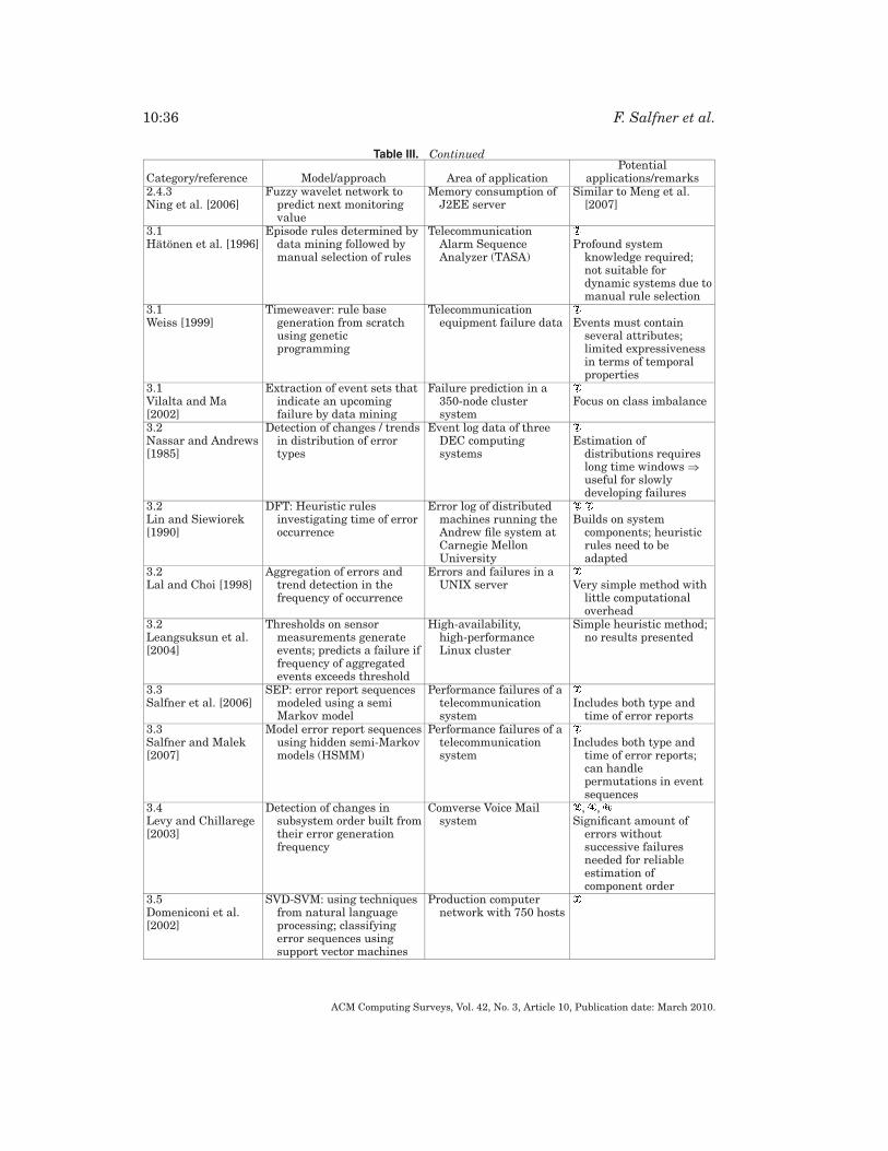
10:36 F. Salfner et al.
Table III. ContinuedPotential
Category/reference Model/approach Area of application applications/remarks2.4.3Ning et al. [2006]
Fuzzy wavelet network topredict next monitoringvalue
Memory consumption ofJ2EE server
Similar to Meng et al.[2007]
3.1Hatonen et al. [1996]
Episode rules determined bydata mining followed bymanual selection of rules
TelecommunicationAlarm SequenceAnalyzer (TASA)
Profound systemknowledge required;not suitable fordynamic systems due tomanual rule selection
3.1Weiss [1999]
Timeweaver: rule basegeneration from scratchusing geneticprogramming
Telecommunicationequipment failure data Events must contain
several attributes;limited expressivenessin terms of temporalproperties
3.1Vilalta and Ma[2002]
Extraction of event sets thatindicate an upcomingfailure by data mining
Failure prediction in a350-node clustersystem
Focus on class imbalance
3.2Nassar and Andrews[1985]
Detection of changes / trendsin distribution of errortypes
Event log data of threeDEC computingsystems
Estimation ofdistributions requireslong time windows ⇒useful for slowlydeveloping failures
3.2Lin and Siewiorek[1990]
DFT: Heuristic rulesinvestigating time of erroroccurrence
Error log of distributedmachines running theAndrew file system atCarnegie MellonUniversity
Builds on systemcomponents; heuristicrules need to beadapted
3.2Lal and Choi [1998]
Aggregation of errors andtrend detection in thefrequency of occurrence
Errors and failures in aUNIX server Very simple method with
little computationaloverhead
3.2Leangsuksun et al.[2004]
Thresholds on sensormeasurements generateevents; predicts a failure iffrequency of aggregatedevents exceeds threshold
High-availability,high-performanceLinux cluster
Simple heuristic method;no results presented
3.3Salfner et al. [2006]
SEP: error report sequencesmodeled using a semiMarkov model
Performance failures of atelecommunicationsystem
Includes both type andtime of error reports
3.3Salfner and Malek[2007]
Model error report sequencesusing hidden semi-Markovmodels (HSMM)
Performance failures of atelecommunicationsystem
Includes both type andtime of error reports;can handlepermutations in eventsequences
3.4Levy and Chillarege[2003]
Detection of changes insubsystem order built fromtheir error generationfrequency
Comverse Voice Mailsystem
, ,Significant amount of
errors withoutsuccessive failuresneeded for reliableestimation ofcomponent order
3.5Domeniconi et al.[2002]
SVD-SVM: using techniquesfrom natural languageprocessing; classifyingerror sequences usingsupport vector machines
Production computernetwork with 750 hosts
ACM Computing Surveys, Vol. 42, No. 3, Article 10, Publication date: March 2010.
Survey of Online Failure Prediction Methods 10:37
(where failure prediction plays a crucial role) will be the key enabler for the next gener-ation of dependability improvement. Researchers have adopted various concepts fromcomputer science resulting in a diverse landscape of approaches to online failure predic-tion. The goal of this survey is to provide an overview of existing approaches includingkey properties and fields of application in order to prepare researchers for the nextchallenge of proactive fault handling: the prediction-based triggering of effective coun-termeasures to enhance system availability by potentially an order of magnitude ormore [Candea et al. 2004; Salfner et al. 2005] by using effective failure avoidance anddowntime minimization methods.
ACKNOWLEDGMENTS
We would like to express our gratitude to the reviewers who provided several constructive comments thathelped to improve this survey.
REFERENCES
ABRAHAM, A. AND GROSAN, C. 2005. Genetic programming approach for fault modeling of electronic hard-ware. In Proceedings of the IEEE Congress on Evolutionary Computation (CEC). Edinburgh, U.K., Vol. 2,1563–1569.
AITCHISON, J. AND DUNSMORE, I. R. 1975. Statistical Prediction Analysis. Cambridge University Press,Cambridge, U.K.
ALTMAN, D. G. 1991. Practical Statistics for Medical Research. CRC Press, Boca Raton, FL.ALTSCHUL, S., GISH, W., MILLER, W., MYERS, E., AND LIPMAN, D. 1990. Basic local alignment search tool. J.
Molec. Biol. 215, 3, 403–410.ANDRZEJAK, A. AND SILVA, L. 2007. Deterministic models of software aging and optimal rejuvenation sched-
ules. In Proceedings of the 10th IEEE/IFIP International Symposium on Integrated Network Manage-ment (IM). 159–168.
AVIZIENIS, A. AND LAPRIE, J.-C. 1986. Dependable computing: From concepts to design diversity. Proc.IEEE 74, 5 (May), 629–638.
AVIZIENIS, A., LAPRIE, J.-C., RANDELL, B., AND LANDWEHR, C. 2004. Basic concepts and taxonomy of dependableand secure computing. IEEE Trans. Dependable Secure Comput. 1, 1, 11–33.
BABAOGLU, O., JELASITY, M., MONTRESOR, A., FETZER, C., LEONARDI, S., VAN MOORSEL A., AND VAN STEEN, M.,EDS. 2005. Self-Star Properties in Complex Information Systems. Lecture Notes in Computer Science,vol. 3460. Springer-Verlag, Berlin, Germany.
BAI, C. G., HU, Q. P., XIE, M., AND NG, S. H. 2005. Software failure prediction based on a Markov Bayesiannetwork model. J. Syst. Softw. 74, 3 (Feb.), 275–282.
BASSEVILLE, M. AND NIKIFOROV, I. 1993. Detection of Abrupt Changes: Theory and Application. Prentice Hall,Englewood Cliffs, NJ.
BERENJI, H., AMETHA, J., AND VENGEROV, D. 2003. Inductive learning for fault diagnosis. In Proceedings ofthe IEEE 12th International Conference on Fuzzy Systems (FUZZ). Vol. 1.
BLISCHKE, W. R. AND MURTHY, D. N. P. 2000. Reliability: Modeling, Prediction, and Optimization. Probabilityand Statistics Series. John Wiley and Sons, New York, NY.
BODIK, P., FRIEDMAN, G., BIEWALD, L., LEVINE, H., CANDEA, G., PATEL, K., TOLLE, G., HUI, J., FOX, A., JORDAN,M. I., AND PATTERSON, D. 2005. Combining visualization and statistical analysis to improve operatorconfidence and efficiency for failure detection and localization. In Proceedings of the IEEE Interna-tional Conference on Autonomic Computing (ICAC). IEEE Computer Society Press, Los Alamitos, CA,89–100.
BROCKLEHURST, S. AND LITTLEWOOD, B. 1996. Techniques for prediction analysis and recalibration. In Hand-book of Software Reliability Engineering, M. R. Lyu, Ed. McGraw-Hill, New York, NY, Chapter 4,119–166.
BROWN, A. AND PATTERSON, D. 2001. Embracing failure: A case for recovery-oriented computing (ROC). InProceedings of the High Performance Transaction Processing Symposium.
CANDEA, G., KAWAMOTO, S., FUJIKI, Y., FRIEDMAN, G., AND FOX, A. 2004. Microreboot—a technique for cheaprecovery. In Proceedings of the 6th Symposium on Operating Systems Design and Implementation.31–44.
ACM Computing Surveys, Vol. 42, No. 3, Article 10, Publication date: March 2010.
10:38 F. Salfner et al.
CANDEA, G., KICIMAN, E., KAWAMOTO, S., AND FOX, A. 2006. Autonomous recovery in componentized Internetapplications. Cluster Comput. 9, 2, 175–190.
CANDEA, G., KICIMAN, E., ZHANG, S., KEYANI, P., AND FOX, A. 2003. Jagr: An autonomous self-recovering appli-cation server. In Proceedings of the 5th International Workshop on Active Middleware Services (Seattle,WA).
CASSIDY, K. J., GROSS, K. C., AND MALEKPOUR, A. 2002. Advanced pattern recognition for detection of complexsoftware aging phenomena in online transaction processing servers. In Proceedings of the Conference onDependable Systems and Networks (DSN). 478–482.
CASTELLI, V., HARPER, R., P., H., HUNTER, S., TRIVEDI, K., VAIDYANATHAN, K., AND ZEGGERT, W. 2001. Proactivemanagement of software aging. IBM J. Res. Develop. 45, 2 (Mar.), 311–332.
CAVAFY, C. P. 1992. But the wise perceive things about to happen. In Collected Poems, G. Savidis, Ed.Princeton University Press, Princeton, NJ.
CHEN, M., ACCARDI, A., LLOYD, J., KICIMAN, E., FOX, A., PATTERSON, D., AND BREWER, E. 2004. Path-based failureand evolution management. In Proceedings of the USENIX/ACM Symposium on Networked SystemsDesign and Implementation (NSDI, San Francisco, CA).
CHEN, M., KICIMAN, E., FRATKIN, E., FOX, A., AND BREWER, E. 2002. Pinpoint: Problem determination in large,dynamic Internet services. In Proceedings of the 2002 International Conference on Dependable Systemsand Networks, IPDS track (DSN). IEEE Computer Society Press, Los Alamitos, CA, 595–604.
CHEN, M.-S., PARK, J. S., AND YU, P. S. 1998. Efficient data mining for path traversal patterns. IEEE Trans.Knowl. Data Eng. 10, 2, 209–221.
CHENG, F., WU, S., TSAI, P., CHUNG, Y., AND YANG, H. 2005. Application cluster service scheme for near-zero-downtime services. In Proceedings of the IEEE International Conference on Robotics and Automation.4062–4067.
CLEVELAND, W. ET AL. 1979. Robust locally weighted regression and smoothing scatterplots. J. Amer. Statist.Assoc. 74, 368, 829–836.
COHEN, W. W. 1995. Fast effective rule induction. In Proceedings of the Twelfth International Conferenceon Machine Learning. 115–123.
COLEMAN, D. AND THOMPSON, C. 2005. Model based automation and management for the adaptive enterprise.In Proceedings of the 12th Annual Workshop of the HP OpenView University Association. 171–184.
CROWELL, J., SHERESHEVSKY, M., AND CUKIC, B. 2002. Using fractal analysis to model software aging. Tech.rep. West Virginia University, Lane Department of CSEE, Morgantown, WV. May.
CSENKI, A. 1990. Bayes predictive analysis of a fundamental software reliability model. IEEE Trans. Re-liab. 39, 2 (Jun.), 177–183.
DAIDONE, A., DI GIANDOMENICO, F., BONDAVALLI, A., AND CHIARADONNA, S. 2006. Hidden Markov models as asupport for diagnosis: Formalization of the problem and synthesis of the solution. In Proceedings of the25th IEEE Symposium on Reliable Distributed Systems (SRDS, Leeds, U.K.).
DEERWESTER, S., DUMAIS, S., FURNAS, G., LANDAUER, T., AND HARSHMAN, R. 1990. Indexing by latent semanticanalysis. J. Amer. Soc. Inform. Sci. 41, 6, 391–407.
DENSON, W. 1998. The history of reliability prediction. IEEE Trans. Reliab. 47, 3 (Sep.), 321–328.DISCENZO, F., UNSWORTH, P., LOPARO, K., AND MARCY, H. 1999. Self-diagnosing intelligent motors: a key en-
abler for nextgeneration manufacturing systems. In Proceedings of the IEEE Colloquium on Intelligentand Self-Validating Sensors.
DOMENICONI, C., PERNG, C.-S., VILALTA, R., AND MA, S. 2002. A classification approach for prediction of targetevents in temporal sequences. In Proceedings of the 6th European Conference on Principles of DataMining and Knowledge Discovery (PKDD’02), T. Elomaa, H. Mannila, and H. Toivonen, Eds. LectureNotes in Artificial Intelligence, vol. 2431. Springer-Verlag, Heidelberg, Germany, 125–137.
DURBIN, R., EDDY, S. R., KROGH, A., AND MITCHISON, G. 1998. Biological Sequence Analysis: ProbabilisticModels of Proteins and Nucleic Acids. Cambridge University Press, Cambridge, U.K.
ELBAUM, S., KANDURI, S., AND AMSCHLER, A. 2003. Anomalies as precursors of field failures. In Proceedingsof the 14th IEEE International Symposium on Software Reliability Engineering (ISSRE). 108–118.
FARR, W. 1996. Software reliability modeling survey. In Handbook of Software Reliability Engineering,M. R. Lyu, Ed. McGraw-Hill, New York, NY, Chapter 3, 71–117.
FAWCETT, T. 2004. ROC graphs: Notes and practical considerations for researchers. Mach. Learn. 31, 1–38.FLACH, P. A. 2004. The many faces of ROC analysis in machine learning. Tutorial at the International
Conference on Machine Learning (ICML’04). http://www.cs.bris.ac.uk/flach/ICML04tutorial/.FU, S. AND XU, C.-Z. 2007. Quantifying temporal and spatial fault event correlation for proactive fail-
ure management. In Proceedings of the IEEE Symposium on Reliable and Distributed Systems(SRDS).
ACM Computing Surveys, Vol. 42, No. 3, Article 10, Publication date: March 2010.
Survey of Online Failure Prediction Methods 10:39
GARG, S., VAN MOORSEL, A., VAIDYANATHAN, K., AND TRIVEDI, K. S. 1998. A methodology for detection andestimation of software aging. In Proceedings of the 9th International Symposium on Software ReliabilityEngineering (ISSRE).
GROSS, K. C., BHARDWAJ, V., AND BICKFORD, R. 2002. Proactive detection of software aging mechanisms inperformance critical computers. In SEW ’02: Proceedings of the 27th Annual NASA Goddard SoftwareEngineering Workshop (SEW-27’02). IEEE Computer Society Press, Los Alamitos, CA.
GROTTKE, M., MATIAS, R., AND TRIVEDI, K. S. 2008. The fundamentals of software aging. In Proceedings ofthe IEEE Workshop on Software Aging and Rejuvenation (Seattle, WA).
GROTTKE, M. AND TRIVEDI, K. 2007. Fighting bugs: Remove, retry, replicate, and rejuvenate. IEEE Comput.40, 107–109.
GUYON, I. AND ELISSEEFF, A. 2003. An introduction to variable and feature selection. J. Mach. Learn. Res. 3,1157–1182. Special Issue on Variable and Feature Selection.
HAMERLY, G. AND ELKAN, C. 2001. Bayesian approaches to failure prediction for disk drives. In Proceedingsof the Eighteenth International Conference on Machine Learning. Morgan Kaufmann Publishers, SanFrancisco, CA, 202–209.
HASTIE, T., TIBSHIRANI, R., AND FRIEDMAN, J. 2001. The Elements of Statistical Learning: Data Mining, Infer-ence, and Prediction. Springer Series in Statistics. Springer Verlag, Berlin, Germany.
HATONEN, K., KLEMETTINEN, M., MANNILA, H., RONKAINEN, P., AND TOIVONEN, H. 1996. Tasa: Telecommuni-cation alarm sequence analyzer, or: How to enjoy faults in your network. In Proceedings of the IEEENetwork Operations and Management Symposium (Kyoto, Japan). Vol. 2., 520–529.
HELLERSTEIN, J. L., ZHANG, F., AND SHAHABUDDIN, P. 1999. An approach to predictive detection for service man-agement. In Proceedings of the 6th IEEE International Symposium on Integrated Network Management.309–322.
HO, D. W. C., ZHANG, P. A., AND XU, J. 2001. Fuzzy wavelet networks for function learning. IEEE Trans.Fuzzy Syst. 9, 1, 200–211.
HOFFMANN, G. A. 2004. Adaptive transfer functions in radial basis function (RBF) networks. In Proceed-ings of the 4th International Conference on Computational Science (ICCS 2004), M. Bubak, G. D. vanAlbada, P. M. A. Sloot, et al., Eds. Lecture Notes in Computer Science, vol. 3037. Springer-Verlag, Berlin,Germany, 682–686.
HOFFMANN, G. A. 2006. Failure Prediction in Complex Computer Systems: A Probabilistic Approach. ShakerVerlag, Herzogexrath, Germany.
HOFFMANN, G. A. AND MALEK, M. 2006. Call availability prediction in a telecommunication system: A datadriven empirical approach. In Proceedings of the 25th IEEE Symposium on Reliable Distributed Systems(SRDS), Leeds, U.K.
HOFFMANN, G. A., SALFNER, F., AND MALEK, M. 2004. Advanced failure prediction in complex softwaresystems. Res. rep. 172, Department of Computer Science, Humboldt University, Berlin, Germany.www.rok.informatik.hu-berlin.de/Members/salfner.
HOFFMANN, G. A., TRIVEDI, K. S., AND MALEK, M. 2006. A best practice guide to resource forecasting for theApache Webserver. In IEEE Proceedings of the 12th International Symposium Pacific Rim DependableComputing (PRDC). University of California, Riverside, Riverside, CA.
HOFFMANN, G. A., TRIVEDI, K. S., AND MALEK, M. 2007. A best practice guide to resource forecasting forcomputing systems. IEEE Trans. Reliab. 56, 4 (Dec.), 615–628.
HORN, P. 2001. Autonomic computing: IBM’s perspective on the state of information technology. Tech. rep.IBM, Yorktown Heights, NY.
HOTELLING, H. 1933. Analysis of a complex of statistical variables into principal components. J. Educat.Psych. 24, 417–441.
HUGHES, G., MURRAY, J., KREUTZ-DELGADO, K., AND ELKAN, C. 2002. Improved disk-drive failure warnings.IEEE Trans. Reliab. 51, 3 (Sep.), 350–357.
IEC: INTERNATIONAL TECHNICAL COMISSION, ED. 2002. Dependability and Quality of Service, 2nd ed. IEC,Geneva, Switzerland, Chapter 191.
IYER, R. K., YOUNG, L. T., AND SRIDHAR, V. 1986. Recognition of error symptoms in large systems. In Pro-ceedings of the 1986 ACM Fall Joint Computer Conference. IEEE Computer Society Press, Los Alamitos,CA, 797–806.
JELINSKI, Z. AND MORANDA, P. 1972. Software reliability research. In Statistical Computer Performance Eval-uation, W. Freiberger, Ed. Academic Press, New York, NY.
KAPADIA, N. H., FORTES, J. A. B., AND BRODLEY, C. E. 1999. Predictive application-performance modelingin a computational gridenvironment. In Procedings of the 8th International IEEE Symposium on HighPerformance Distributed Computing. 47–54.
ACM Computing Surveys, Vol. 42, No. 3, Article 10, Publication date: March 2010.
10:40 F. Salfner et al.
KICIMAN, E. AND FOX, A. 2005. Detecting application-level failures in component-based Internet services.IEEE Trans. Neural Netw. 16, 5 (Sep.), 1027–1041.
KORBICZ, J., KOSCIELNY, J. M., KOWALCZUK, Z., AND CHOLEWA, W., EDS. 2004. Fault Diagnosis: Models, ArtificialIntelligence, Applications. Springer-Verlag, Berlin, Germany.
LAL, R. AND CHOI, G. 1998. Error and failure analysis of a unix server. In Proceedings of the IEEE 3rdInternational High-Assurance Systems Engineering Symposium (HASE). IEEE Computer Society Press,Los Alamitos, CA, 232–239.
LAPRIE, J.-C. AND KANOUN, K. 1996. Software reliability and system reliability. In Handbook of SoftwareReliability Engineering, M. R. Lyu, Ed. McGraw-Hill, New York, NY, Chapter 2, 27–69.
LEANGSUKSUN, C., LIU, T., RAO, T., SCOTT, S., AND LIBBY, R. 2004. A failure predictive and policy-based highavailability strategy for Linux high performance computing cluster. In Proceedings of the 5th LCI Inter-national Conference on Linux Clusters: The HPC Revolution. 18–20.
LEVY, D. AND CHILLAREGE, R. 2003. Early warning of failures through alarm analysis—a case study intelecom voice mail systems. In ISSRE ’03: Proceedings of the 14th International Symposium on SoftwareReliability Engineering. IEEE Computer Society Press, Los Alamitos, CA.
LI, L., VAIDYANATHAN, K., AND TRIVEDI, K. S. 2002. An approach for estimation of software aging in a Webserver. In Proceedings of the Intenational Symposium on Empirical Software Engineering (ISESE, Nara,Japan).
LIANG, Y., ZHANG, Y., SIVASUBRAMANIAM, A., JETTE, M., AND SAHOO, R. 2006. Bluegene/l failure analysis andprediction models. In Proceedings of the IEEE International Conference on Dependable Systems andNetworks (DSN). 425–434.
LIN, T.-T. Y. AND SIEWIOREK, D. P. 1990. Error log analysis: Statistical modeling and heuristic trend analysis.IEEE Trans. Reliab. 39, 4 (Oct.), 419–432.
LUNZE, J. 2003. Automatisierungstechnik, 1st ed. Oldenbourg, Munich, Germany.LYU, M. R., ED. 1996. Handbook of Software Reliability Engineering. McGraw-Hill, New York, NY.MANNING, C. D. AND SCHUTZE, H. 1999. Foundations of Statistical Natural Language Processing. MIT Press,
Cambridge, MA.MELLIAR-SMITH, P. M. AND RANDELL, B. 1977. Software reliability: The role of programmed exception han-
dling. SIGPLAN Not. 12, 3, 95–100.MENG, H., DI HOU, Y., AND CHEN, Y. 2007. A rough wavelet network model with genetic algorithm and its
application to aging forecasting of application server. In Procedings of the IEEE International Conferenceon Machine Learning and Cybernetics. Vol. 5.
MUNDIE, C., DE VRIES, P., HAYNES, P., AND CORWINE, M. 2002. Trustworthy computing. Tech. rep., MicrosoftCorp., Redmond, WA. Oct.
MURRAY, J., HUGHES, G., AND KREUTZ-DELGADO, K. 2003. Hard drive failure prediction using non-parametricstatistical methods. In Proceedings of ICANN/ICONIP.
MUSA, J. D., IANNINO, A., AND OKUMOTO, K. 1987. Software Reliability: Measurement, Prediction, Application.McGraw-Hill, New York, NY.
NASSAR, F. A. AND ANDREWS, D. M. 1985. A methodology for analysis of failure prediction data. In Proceedingsof the IEEE Real-Time Systems Symposium. 160–166.
NEEDLEMAN, S. B. AND WUNSCH, C. D. 1970. A general method applicable to the search for similarities in theamino acid sequence of two proteins. J. Molec. Biol. 48, 3, 443–53.
NEVILLE, S. W. 1998. Approaches for early fault detection in large scale engineering plants. Ph.D. disser-tation, University of Victoria, Victoria, B.C., Canada.
NING, M. H., YONG, Q., DI, H., YING, C., AND ZHONG, Z. J. 2006. Software aging prediction model based on fuzzywavelet network with adaptive genetic algorithm. In Proceedings of the IEEE 18th IEEE InternationalConference on Tools with Artificial Intelligence (ICTAI). IEEE Computer Society Press, Los Alamitos,CA, 659–666.
PARNAS, D. L. 1994. Software aging. In Proceedings of the 16th IEEE International Conference on SoftwareEngineering (ICSE). IEEE Computer Society Press, Los Alamitos, CA, 279–287.
PATTERSON, D. A., BROWN, A., BROADWELL, P., CANDEA, G., CHEN, M., CUTLER, J., ENRIQUEZ, P., FOX, A., KICIMAN,E., MERZBACHER, M., OPPENHEIMER, D., SASTRY, N., TETZLAFF, W., TRAUPMAN, J., AND TREUHAFT, N. 2002.Recovery-oriented computing (ROC): Motivation, definition, techniques, and case studies. Tech. rep.UCB//CSD-02-1175. Computer Science Department, University of California, Berkeley, Berkeley, CA.March.
PAWLAK, Z., WONG, S. K. M., AND ZIARKO, W. 1988. Rough sets: Probabilistic versus deterministic approach.Internat. J. Man-Mach. Stud. 29, 81–95.
ACM Computing Surveys, Vol. 42, No. 3, Article 10, Publication date: March 2010.

Survey of Online Failure Prediction Methods 10:41
PETTITT, A. 1977. Testing the normality of several independent samples using the anderson-darling statis-tic. Appl. Statist. 26, 2, 156–161.
PFEFFERMAN, J. AND CERNUSCHI-FRIAS, B. 2002. A nonparametric nonstationary procedure for failure predic-tion. IEEE Trans. Reliab. 51, 4 (Dec.), 434–442.
PIZZA, M., STRIGINI, L., BONDAVALLI, A., AND DI GIANDOMENICO, F. 1998. Optimal discrimination be-tween transient and permanent faults. In Proceedings of the IEEE 3rd International High-Assurance Systems Engineering Symposium (HASE). IEEE Computer Society Press, Los Alamitos, CA,214–223.
QUINLAN, J. 1990. Learning logical definitions from relations. Mach. Learn. 5, 3, 239–266.QUINLAN, J. 1993. C4. 5: Programs for Machine Learning. Morgan Kaufmann, San Francisco, CA.RABINER, L. R. 1989. A tutorial on hidden Markov models and selected applications in speech recognition.
Proc. IEEE 77, 2 (Feb.), 257–286.ROVNYAK, S., KRETSINGER, S., THORP, J., AND BROWN, D. 1994. Decision trees for real-time transient stability
prediction. IEEE Trans. Power Syst. 9, 3, 1417–1426.SAHNER, R. A., TRIVEDI, K. S., AND PULIAFITO, A. 1996. Performance and Reliability Analysis of Computer
Systems: An Example-Based Approach Using the SHARPE Software Package (The Red Book). KluwerAcademic Publishers, Dordrecht, The Netherlands.
SAHOO, R. K., OLINER, A. J., RISH, I., GUPTA, M., MOREIRA, J. E., MA, S., VILALTA, R., AND SIVASUBRAMANIAM, A.2003. Critical event prediction for proactive management in large-scale computer clusters. In Proceed-ings of the 9th ACM SIGKDD International Conference on Knowledge Discovery and Data Mining (KDD).ACM Press, New York, NY, 426–435.
SALFNER, F. 2006. Modeling event-driven time series with generalized hidden semi-Markov models. Tech.rep. 208. Department of Computer Science, Humboldt-Universitat zu Berlin, Berlin, Germany.http://edoc.hu-berlin.de/docviews/abstract.php?id=27653.
SALFNER, F. 2008. Event-based Failure Prediction: An Extended Hidden Markov Model Approach.dissertation.de—Verlag im Internet GmbH, Berlin, Germany. http://www.rok.informatik.hu-berlin.de/Members/salfner/publications/salfner08event-based.pdf.
SALFNER, F., HOFFMANN, G. A., AND MALEK, M. 2005. Prediction-based software availability enhancement. InSelf-Star Properties in Complex Information Systems, O. Babaoglu, M. Jelasity, A. Montresor, C. Fetzer,S. Leonardi, van Moorsel A., and M. van Steen, Eds. Lecture Notes in Computer Science, vol. 3460.Springer-Verlag, Berlin, Germany.
SALFNER, F. AND MALEK, M. 2007. Using hidden semi-Markov models for effective online failure pre-diction. In Proceedings of the IEEE 26th International Symposium on Reliable Distributed Systems(SRDS).
SALFNER, F., SCHIESCHKE, M., AND MALEK, M. 2006. Predicting failures of computer systems: A case studyfor a telecommunication system. In Proceedings of the IEEE International Parallel and DistributedProcessing Symposium (IPDPS, Rhodes Island, Greece).
SALFNER, F., TSCHIRPKE, S., AND MALEK, M. 2004. Comprehensive logfiles for autonomic systems. In Pro-ceedings of the IEEE International Parallel and Distributed Processing Symposium (IPDPS), Workshopon Fault-Tolerant Parallel, Distributed and Network-Centric Systems (FTPDS). IEEE Computer SocietyPress, Los Alamitos, CA.
SEN, P. K. 1968. Estimates of the regression coefficient based on Kendall’s tau. J. Amer. Statist.Assoc. 63, 324 (Dec.), 1379–1389.
SHERESHEVSKY, M., CROWELL, J., CUKIC, B., GANDIKOTA, V., AND LIU, Y. 2003. Software aging and multifrac-tality of memory resources. In Proceedings of the International Conference on Dependable Systems andNetworks (DSN). IEEE Computer Society Press, Los Alamitos, CA, 721–730.
SIEWIOREK, D. P. AND SWARZ, R. S. 1998. Reliable Computer Systems, 3rd ed. A. K. Peters, Ltd., Wellesley,MA.
SINGER, R. M., GROSS, K. C., HERZOG, J. P., KING, R. W., AND WEGERICH, S. 1997. Model-based nuclear powerplant monitoring and fault detection: Theoretical foundations. In Proceedings of the Conference on Intel-ligent System Application to Power Systems (ISAP, Seoul, Korea). 60–65.
SMITH, T. AND WATERMAN, M. 1981. Identification of common molecular subsequences. J. Molec. Biol. 147,195–197.
SRIKANT, R. AND AGRAWAL, R. 1996. Mining sequential patterns: Generalizations and performance improve-ments. In Proceedings of the 5th International Conference on Extending Database Technology, EDBT,P. M. G. Apers, M. Bouzeghoub, and G. Gardarin, Eds. Lecture Notes in Computer Science, vol. 1057.Springer-Verlag, Berlin, Germany, 3–17.
ACM Computing Surveys, Vol. 42, No. 3, Article 10, Publication date: March 2010.
10:42 F. Salfner et al.
TANG, D. AND IYER, R. 1993. Dependability measurement and modeling of a multicomputer system. IEEETrans. Comput. 42, 1 (Jan.), 62–75.
TROUDET, T., MERRILL, W., CENTER, N., AND CLEVELAND, O. 1990. A real time neural net estimator of fa-tigue life. In Proceedings of the IEEE International Joint Conference on Neural Networks (IJCNN).59–64.
TSAO, M. M. AND SIEWIOREK, D. P. 1983. Trend analysis on system error files. In Proceedings of the 13thInternational Symposium on Fault-Tolerant Computing (Milano, Italy). 116–119.
TURNBULL, D. AND ALLDRIN, N. 2003. Failure prediction in hardware systems. Tech. rep. University ofCalifornia, San Diego, CA. http://www.cs.ucsd.edu/~dturnbul/Papers/ServerPrediction.pdf.
ULERICH, N. AND POWERS, G. 1988. On-line hazard aversion and fault diagnosis in chemical processes: Thedigraph+fault-tree method. IEEE Trans. Reliab. 37, 2 (Jun.), 171–177.
VAIDYANATHAN, K. AND TRIVEDI, K. S. 1999. A measurement-based model for estimation of resource exhaus-tion in operational software systems. In Proceedings of the International Symposium on Software Reli-ability Engineering (ISSRE).
VAN RIJSBERGEN, C. J. 1979. Information Retrieval, second ed. Butterworth, London, U.K.VAPNIK, V. N. 1995. The Nature of Statistical Learning Theory. Springer Verlag, New York, NY.VESELY, W., GOLDBERG, F. F., ROBERTS, N. H., AND HAASL, D. F. 1981. Fault tree handbook. Tech. rep. NUREG-
0492. U.S. Nuclear Regulatory Commission, Washington, DC.VILALTA, R., APTE, C. V., HELLERSTEIN, J. L., MA, S., AND WEISS, S. M. 2002. Predictive algorithms in the
management of computer systems. IBM Syst. J. 41, 3, 461–474.VILALTA, R. AND MA, S. 2002. Predicting rare events in temporal domains. In Proceedings of the IEEE
International Conference on Data Mining (ICDM). IEEE Computer Society Press, Los Alamitos, CA,474–482.
WARD, A., GLYNN, P., AND RICHARDSON, K. 1998. Internet service performance failure detection.SIGMETRICS Perform. Eval. Rev. 26, 3, 38–43.
WARD, A. AND WHITT, W. 2000. Predicting response times in processor-sharing queues. In Proceedings of theFields Institute Conference on Communications Networks, P. W. Glynn, D. J. MacDonald, and S. J. Turner,Eds.
WEISS, G. 1999. Timeweaver: A genetic algorithm for identifying predictive patterns in sequences ofevents. In Proceedings of the Genetic and Evolutionary Computation Conference. Morgan Kaufmann,San Francisco, CA, 718–725.
WEISS, G. 2002. Predicting telecommunication equipment failures from sequences of network alarms. InHandbook of Knowledge Discovery and Data Mining, W. Kloesgen and J. Zytkow, Eds. Oxford UniversityPress, Oxford, U.K., 891–896.
WONG, K. C. P., RYAN, H., AND TINDLE, J. 1996. Early warning fault detection using artificial intelligentmethods. In Proceedings of the Universities Power Engineering Conference.
ZIPF, G. K. 1949. Human Behavior and the Principle of Least Effort: An Introduction to Human Ecology.Addison-Wesley Press, Cambridge, MA.
Received July 2007; revised June 2008; accepted October 2008
ACM Computing Surveys, Vol. 42, No. 3, Article 10, Publication date: March 2010.