TransferLearningforImprovingModelPredictionsinRoboticSystems

Pooyan Jamshidi, Miguel Velez, Christian KästnerNorbert Siegmund, Prasad Kawthekar

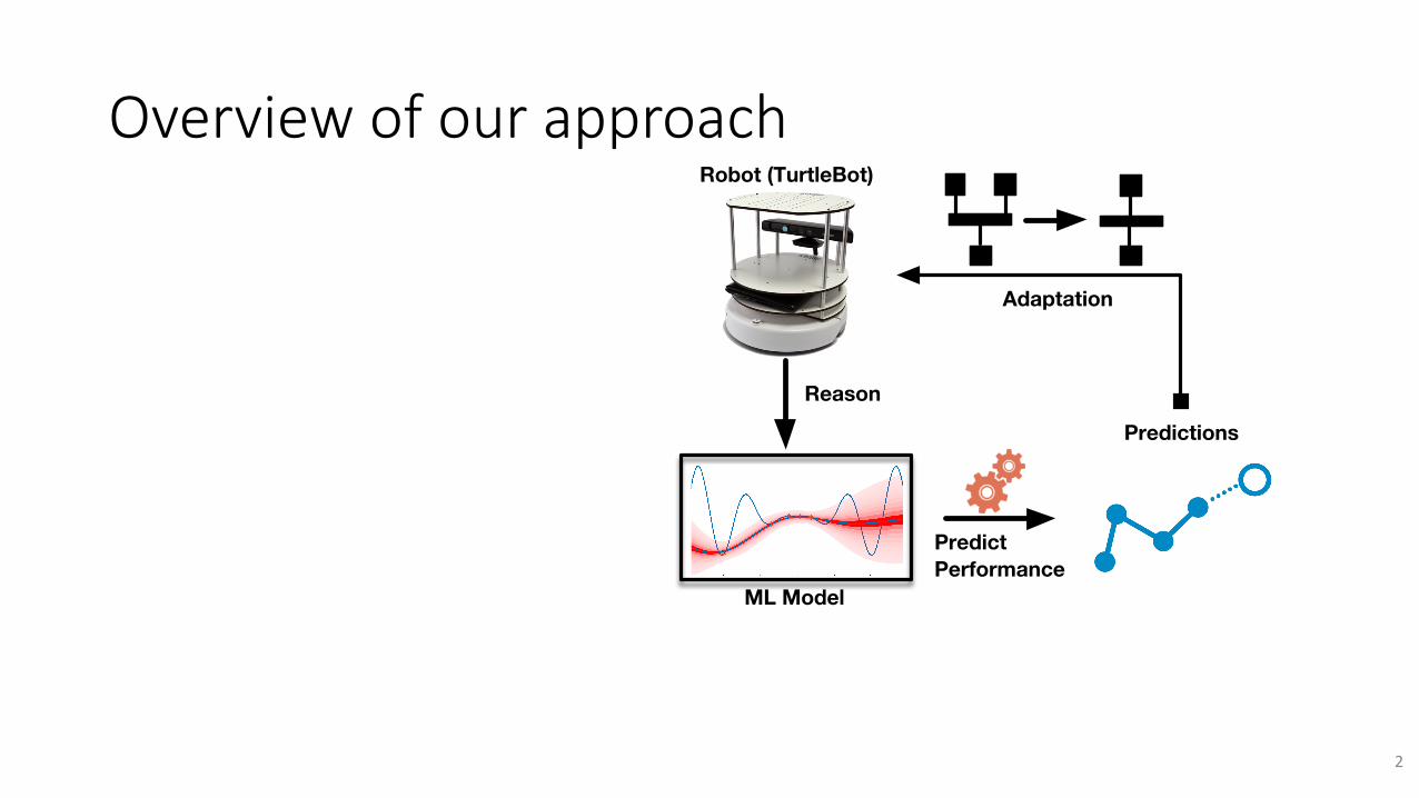
Overviewofourapproach

ML Model

Learn Model

MeasureMeasure

DataSourceTarget

Simulator (Gazebo) Robot (TurtleBot)

Predict Performance

Predictions

Adaptation

Reason

2

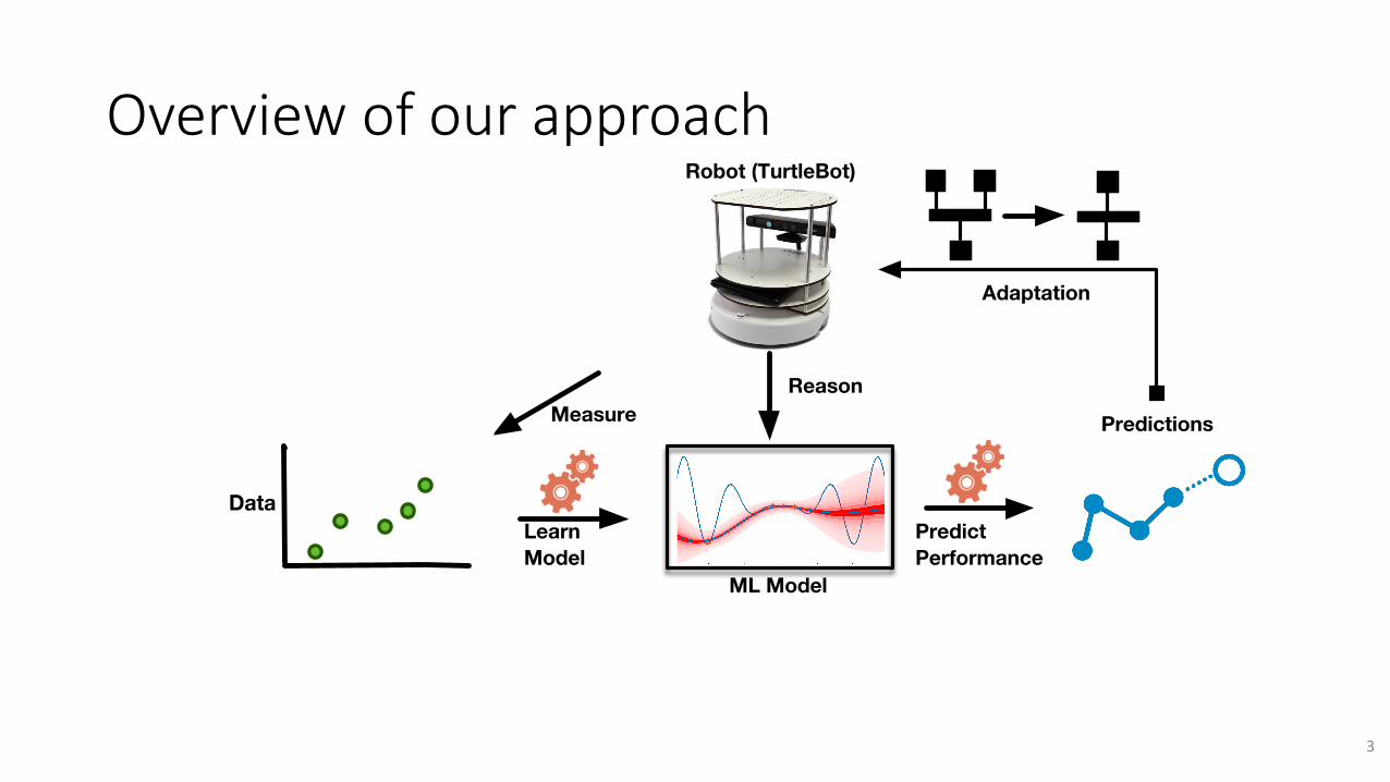
Overviewofourapproach

ML Model

Learn Model

MeasureMeasure

DataSourceTarget

Simulator (Gazebo) Robot (TurtleBot)

Predict Performance

Predictions

Adaptation

Reason

Data

3

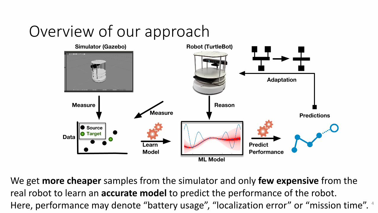
Overviewofourapproach

Wegetmore cheaper samplesfromthesimulatorandonlyfewexpensivefromtherealrobottolearnanaccuratemodeltopredicttheperformanceoftherobot.Here,performancemaydenote“batteryusage”,“localizationerror”or“missiontime”.

ML Model

Learn Model

MeasureMeasure

DataSourceTarget

Simulator (Gazebo) Robot (TurtleBot)

Predict Performance

Predictions

Adaptation

Reason

4

Traditionalmachinelearningvs.transferlearningSourceDomain

(cheap)TargetDomain(expensive)

LearningAlgorithm

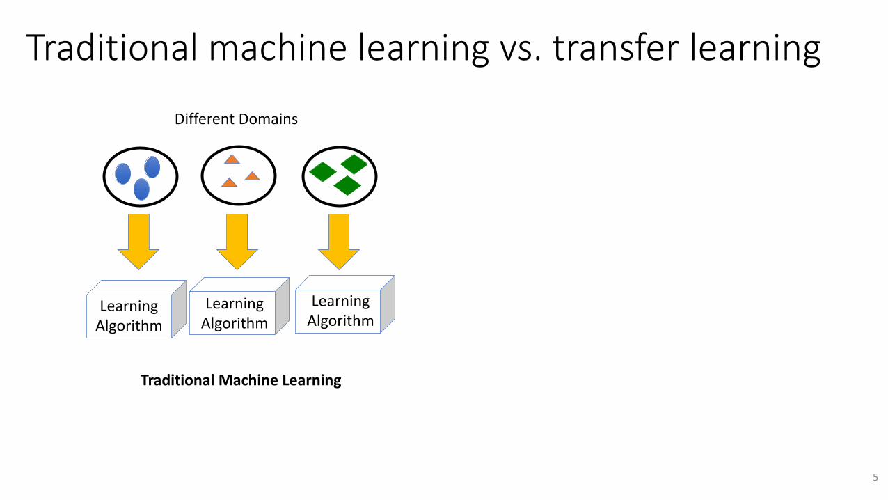
DifferentDomains

LearningAlgorithm

LearningAlgorithm

LearningAlgorithm

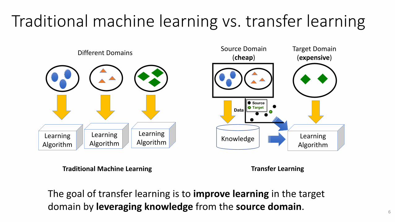
TraditionalMachineLearning TransferLearning

Knowledge

DataSourceTarget

5

Traditionalmachinelearningvs.transferlearningSourceDomain

(cheap)TargetDomain(expensive)

LearningAlgorithm

DifferentDomains

LearningAlgorithm

LearningAlgorithm

LearningAlgorithm

TraditionalMachineLearning TransferLearning

Thegoaloftransferlearningistoimprovelearninginthetargetdomainbyleveragingknowledgefromthesourcedomain.

Knowledge

DataSourceTarget

6

PerformancepredictionforCoBot

5 10 15 20 25

5

10

15

20

25

14

16

18

20

22

24

5 10 15 20 25

5

10

15

20

25

8

10

12

14

16

18

20

22

24

26

5 10 15 20 25

5

10

15

20

25

5

10

15

20

25

30CPU usage [%] CPU usage [%]

(a) (b)

(c) (d)

Prediction without transfer learning

5 10 15 20 25

5

10

15

20

25

10

15

20

25

Prediction with transfer learning

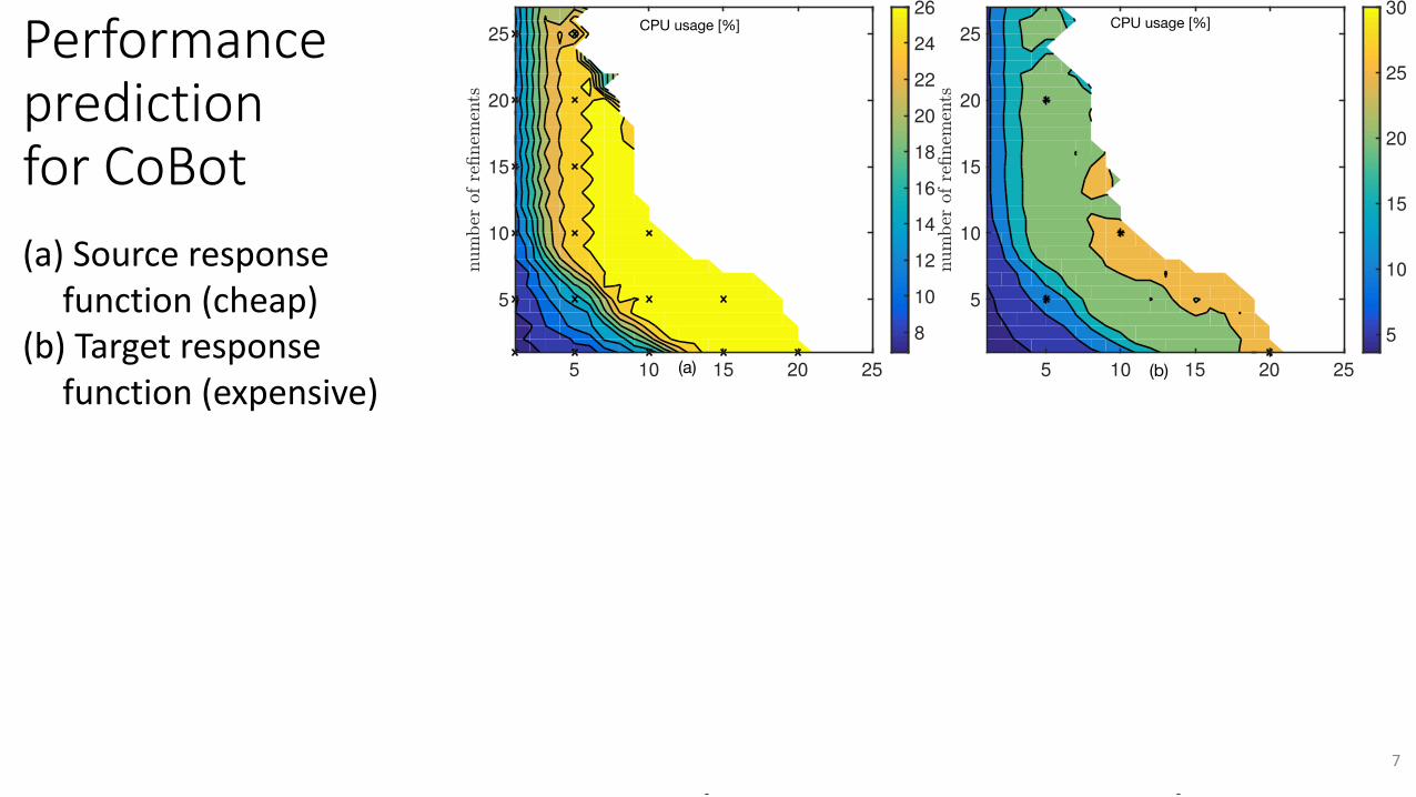
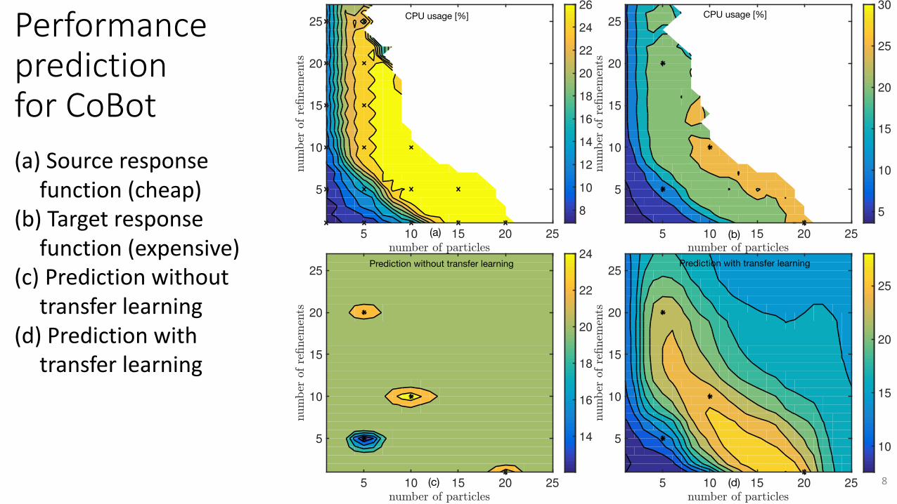
(a) Sourceresponsefunction(cheap)

(b) Targetresponsefunction(expensive)

7

PerformancepredictionforCoBot

5 10 15 20 25

5

10

15

20

25

14

16

18

20

22

24

5 10 15 20 25

5

10

15

20

25

8

10

12

14

16

18

20

22

24

26

5 10 15 20 25

5

10

15

20

25

5

10

15

20

25

30CPU usage [%] CPU usage [%]

(a) (b)

(c) (d)

Prediction without transfer learning

5 10 15 20 25

5

10

15

20

25

10

15

20

25

Prediction with transfer learning

(a) Sourceresponsefunction(cheap)

(b) Targetresponsefunction(expensive)

(c) Predictionwithouttransferlearning

(d) Predictionwithtransferlearning

8

Predictionaccuracyandmodelreliability

2

2

2

2

2

2

2

2

2

44

4

4

6

6

68

8 1012

14 16

1 2 3 4 5 6 7 8 9 100

10

20

30

40

50

60

70

80

90

100

5

5

5

55

5

5

55

1010

10

10

1515

15

20

20

25303540

1 2 3 4 5 6 7 8 9 100

10

20

30

40

50

60

70

80

90

100

(a) (b)

0.5 0.5 0.51 1 1

1.5 1.5 1.5

2

2 2

2.5 2.52.5

33

3

3

3.5

3.5

3.5

3.5

4

4 4

4

4

4.5 4.5 4.5

5

1 2 3 4 5 6 7 8 9 100

10

20

30

40

50

60

70

80

90

100

0.005 0.005 0.0050.01 0.01 0.01

0.015 0.015 0.0150.02 0.02 0.02 0

.02

0.0

25

0.025

0.025 0.025

0.025

0.02

50.025

0.0

3

0.03

0.03

0.0

3

0.03

0.0

30.03

0.035

0.0

35 0.0

35

0.04

1 2 3 4 5 6 7 8 9 100

10

20

30

40

50

60

70

80

90

100

(c) (d)

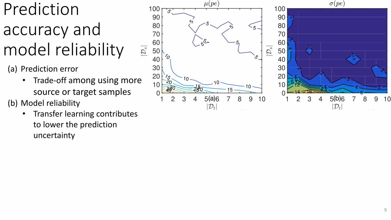
(a) Predictionerror• Trade-offamongusingmore

sourceortargetsamples(b) Modelreliability

• Transferlearningcontributestolowerthepredictionuncertainty

9

Predictionaccuracyandmodelreliability

2

2

2

2

2

2

2

2

2

44

4

4

6

6

68

8 1012

14 16

1 2 3 4 5 6 7 8 9 100

10

20

30

40

50

60

70

80

90

100

5

5

5

55

5

5

55

1010

10

10

1515

15

20

20

25303540

1 2 3 4 5 6 7 8 9 100

10

20

30

40

50

60

70

80

90

100

(a) (b)

0.5 0.5 0.51 1 1

1.5 1.5 1.5

2

2 2

2.5 2.52.5

33

3

3

3.5

3.5

3.5

3.5

4

4 4

4

4

4.5 4.5 4.5

5

1 2 3 4 5 6 7 8 9 100

10

20

30

40

50

60

70

80

90

100

0.005 0.005 0.0050.01 0.01 0.01

0.015 0.015 0.0150.02 0.02 0.02 0

.02

0.0

25

0.025

0.025 0.025

0.025

0.02

50.025

0.0

3

0.03

0.03

0.0

3

0.03

0.0

30.03

0.035

0.0

35 0.0

35

0.04

1 2 3 4 5 6 7 8 9 100

10

20

30

40

50

60

70

80

90

100

(c) (d)

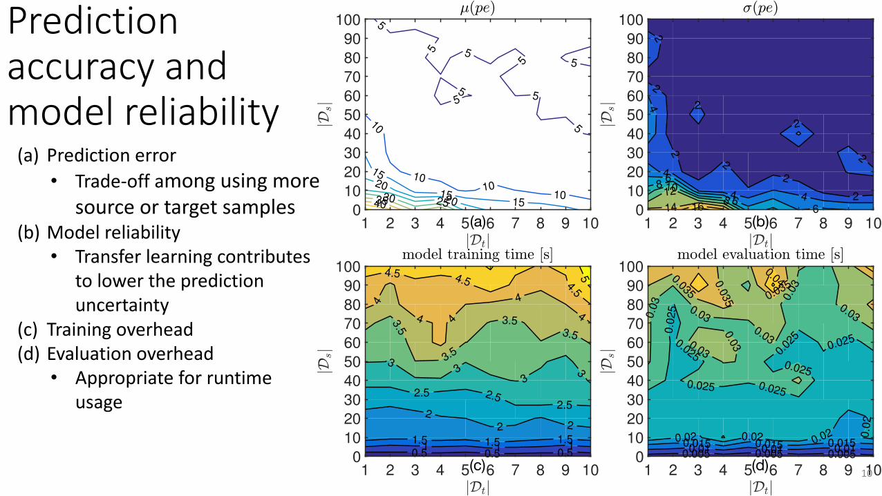
(a) Predictionerror• Trade-offamongusingmore

sourceortargetsamples(b) Modelreliability

• Transferlearningcontributestolowerthepredictionuncertainty

(c) Trainingoverhead(d) Evaluationoverhead

• Appropriateforruntimeusage

10

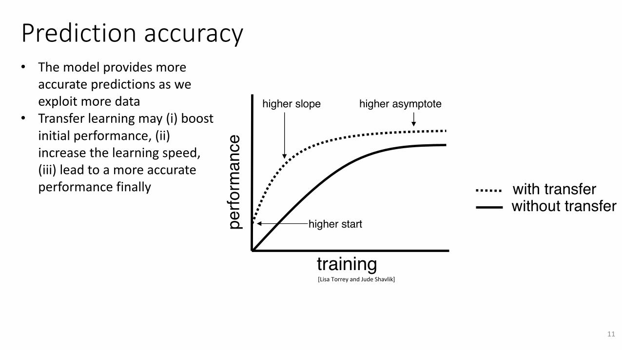
Predictionaccuracy• Themodelprovidesmore

accuratepredictionsasweexploitmoredata

• Transferlearningmay(i)boostinitialperformance,(ii)increasethelearningspeed,(iii)leadtoamoreaccurateperformancefinally

Given

Data

Source-TaskKnowledge

Learn

Target Task

Fig. 1. Transfer learning is machine learning with an additional source of informationapart from the standard training data: knowledge from one or more related tasks.

The goal of transfer learning is to improve learning in the target task byleveraging knowledge from the source task. There are three common measures bywhich transfer might improve learning. First is the initial performance achievablein the target task using only the transferred knowledge, before any further learn-ing is done, compared to the initial performance of an ignorant agent. Second isthe amount of time it takes to fully learn the target task given the transferredknowledge compared to the amount of time to learn it from scratch. Third is thefinal performance level achievable in the target task compared to the final levelwithout transfer. Figure 2 illustrates these three measures.

If a transfer method actually decreases performance, then negative transferhas occurred. One of the major challenges in developing transfer methods isto produce positive transfer between appropriately related tasks while avoidingnegative transfer between tasks that are less related. A section of this chapterdiscusses approaches for avoiding negative transfer.

When an agent applies knowledge from one task in another, it is often nec-essary to map the characteristics of one task onto those of the other to specifycorrespondences. In much of the work on transfer learning, a human providesthis mapping, but some methods provide ways to perform the mapping auto-matically. Another section of the chapter discusses work in this area.

perfo

rman

ce

training

with transferwithout transfer

higher start

higher slope higher asymptote

Fig. 2. Three ways in which transfer might improve learning.

2

[LisaTorreyandJudeShavlik]

11

Currentpriority

Wehavelookedintotransferlearningfromsimulatortorealrobot,butnow,weconsiderthefollowingscenarios:• Workloadchange(Newtasksormissions,newenvironmentalconditions)• Infrastructurechange(NewIntelNUC,newCamera,newSensors)• Codechange(newversionsofROS,newlocalizationalgorithm)

12

Backupslides

13

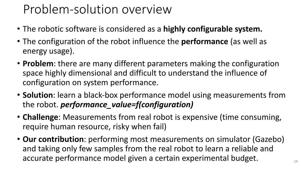
Problem-solutionoverview• Theroboticsoftwareisconsideredasahighlyconfigurablesystem.• Theconfigurationoftherobotinfluencetheperformance (aswellasenergyusage).• Problem:therearemanydifferentparametersmakingtheconfigurationspacehighlydimensionalanddifficulttounderstandtheinfluenceofconfigurationonsystemperformance.• Solution:learnablack-boxperformancemodelusingmeasurementsfromtherobot.performance_value=f(configuration)• Challenge:Measurementsfromrealrobotisexpensive(timeconsuming,requirehumanresource,riskywhenfail)• Ourcontribution:performingmostmeasurementsonsimulator(Gazebo)andtakingonlyfewsamplesfromtherealrobottolearnareliableandaccurateperformancemodelgivenacertainexperimentalbudget. 14

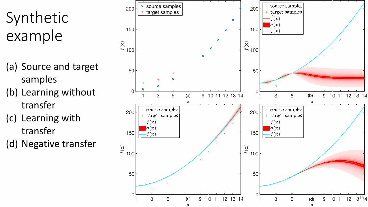
Syntheticexample

(a) Sourceandtargetsamples

(b) Learningwithouttransfer

(c) Learningwithtransfer

(d) Negativetransfer

1 3 5 9 10 11 12 13 140

50

100

150

200source samplestarget samples

(a) (b)

(c) (d) 15

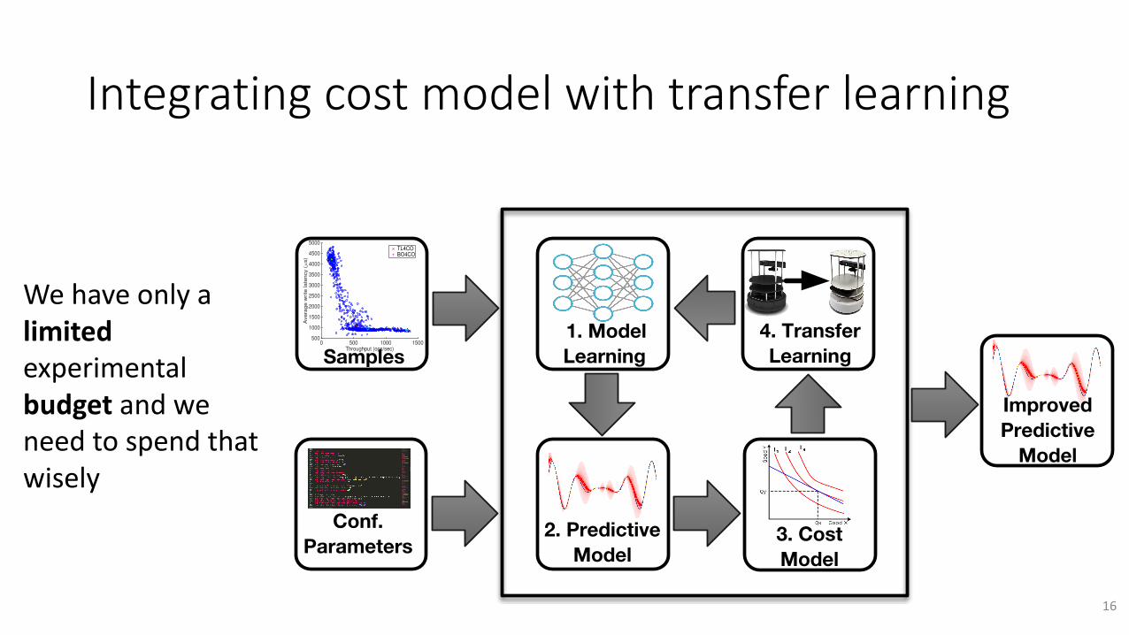
Integratingcostmodelwithtransferlearning

1. Model Learning

2. Predictive Model

4. Transfer Learning

3. Cost Model

ImprovedPredictive

Model

Conf.Parameters

Samples0 500 1000 1500

Throughput (ops/sec)

500

1000

1500

2000

2500

3000

3500

4000

4500

5000

Avera

ge w

rite

late

ncy (µ

s)

TL4COBO4CO

Wehaveonlyalimitedexperimentalbudget andweneedtospendthatwisely

16

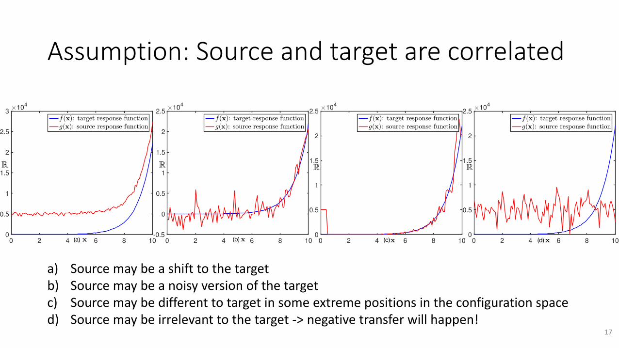
Assumption:Sourceandtargetarecorrelated

0 2 4 6 8 100

0.5

1

1.5

2

2.510

4

0 2 4 6 8 100

0.5

1

1.5

2

2.5

310

4

0 2 4 6 8 100

0.5

1

1.5

2

2.510

4

(a) (b) (c)

0 2 4 6 8 100

0.5

1

1.5

2

2.5

310

4

(d)

0 2 4 6 8 100

0.5

1

1.5

2

2.5

310

4

0 2 4 6 8 10-0.5

0

0.5

1

1.5

2

2.510

4

0 2 4 6 8 100

0.5

1

1.5

2

2.5

310

4

0 2 4 6 8 100

0.5

1

1.5

2

2.5

310

4

gain from the relationship of simulation samples and the fewones on real system to train a performance model that is moreaccurate at less costly comparing with the situation where werely only on observations from real systems.

B. ChallengesAlthough we can take relatively cheap samples from simula-

tion, it is impractical and naive to exhaustively run simulationenvironments for all possible combination of configurationoptions:

• The configuration space of just 20 parameters with binaryoptions for each comprises of 220 = 1m possible options.Note that real systems typically have much larger config-uration parameters. But even for this small configurationspace, if we spend just one minute for collecting eachsample, it will take 694 days (⇡ 2 years) to perform anexhaustive sampling. Therefore, we can sample only asubset of this space, and we need to do this purposefully.

• Not all samples from a simulator reflects the real behaviorand, as a result, would be useful for learning a perfor-mance model. More specifically, the measurements fromsimulators typically contain noise and for some configu-ration, the data may not have any relationship with thedata we may observe on the real system. Therefore, if welearn a model based on these data, it becomes inaccurateand far from real system behavior and any reasoningbased on the model predictions becomes misleading orineffective. This is the case of negative transfer and wewill demonstrate specific cases where a negative transferhappens.

• Often, there exist different sources of data (e.g., differentsimulators, different versions of a system) that we canlearn from. However, too many training samples causelong training time. Since the learned model may be usedin some time constrained environments (e.g., runtimedecision making in a feedback loop for robots), it isimportant to select the sources purposefully.

C. Problem formulation: Model learningIn order to introduce the concepts in our approach precisely

and concisely, we define the model learning problem usingmathematical notation. Let X

i

indicate the i-th configurationparameter, which ranges in a finite domain Dom(X

i

). Ingeneral, X

i

may either indicate (i) an integer variable such asthe number of iterative refinements in a localization algorithmor (ii) a categorical variable such as sensor names or binaryoptions (e.g., local vs global localization method). There-fore, the configuration space is mathematically a Cartesianproduct of all of the domains of the parameters of interestX = Dom(X1)⇥ · · ·⇥Dom(X

d

).A configuration x resides in the design parameter space

x 2 X. A black-box response function f : X ! R isused to build a performance model given some observationsof the system performance under different settings, D ✓ X.In practice, though, such measurements may contain noise,i.e., y

i

= f(xi

) + ✏

i

where ✏

i

⇠ N (0,�i

). In other words,a performance model is simply a function (mapping) fromconfiguration space to a measurable performance metric thatproduces interval-scaled data (here we assume it produces real

numbers). Note that we can learn a model for all measurableattributes (including accuracy, safety), but here we mostly trainpredictive models on performance attributes (e.g., responsetime, throughput, CPU utilization).

The goal here is to learn a reliable regression model, f̂(·)that can predict the performance of the system, f(·), given alimited number of measurements taken from the real systemto minimize the prediction error:

arg minx2D

pe = |f̂(x)� f(x)| (1)

In order to solve the problem above, we assume f(·) isreasonably smooth, but where otherwise little is known aboutthe response function. Intuitively, we expect that for “near-by”input points x and x

0 their corresponding output points y andy

0 to be “near-by” as well. This allows us to build a modelusing black-box models that can predict unobserved values.

D. State-of-the-artIn literature, this problem has been approached from two

different standpoints: (i) sampling strategies and (ii) learningmethods.

1) Model learning: Sampling. Random sampling has beenused to collect unbiased observations in computer-based exper-iments. However, based on our experience, random samplingmay require a large number of samples to build an accuratemodel, and since the overall tuning time is an importantconsideration in an auto-tuner, a long training time can reduceits effectiveness. More intelligent sampling approaches (suchas Latin Hypercube, Box Behnken, and Plackett Burman) havebeen developed in statistics and machine learning community,in which experimental designs have been developed to ensurecertain statistical properties [22]. The aim of these differentexperimental design is to ensure that we gain high level ofinformation from sparse sampling (partial design) in highdimensional spaces. Relevant to software engineering commu-nity, several approaches tried different experimental designsfor highly configurable software [14] and some even considercost as an explicit factor to determine optimal sampling [26].

Recently, researchers have tried novel way of sampling witha feedback embedded inside the process where new samplesare derived based on information gain from previous set ofsamples. Recursive Random Sampling (RRS) [33] integratesa restarting mechanism into the random sampling to achievehigh search efficiency. Smart Hill Climbing (SHC) [32] inte-grates the importance sampling with Latin Hypercube Design(lhd). SHC estimates the local regression at each potentialregion, then it searches toward the steepest descent direction.An approach based on direct search [35] forms a simplex inthe parameter space by a number of samples, and iterativelyupdates a simplex through a number of well-defined operationsincluding reflection, expansion, and contraction to guide thesample generation. Quick Optimization via Guessing (QOG)in [23] speeds up the optimization process exploiting someheuristics to filter out sub-optimal configurations. Some recentwork [34] exploited a characteristic of the response surface ofthe configurable software to learn Fourier sparse functions byonly a small sample size. Another approach also exploited thisfact, but iteratively construct a regression model representingperformance influences in an active learning process.

gain from the relationship of simulation samples and the fewones on real system to train a performance model that is moreaccurate at less costly comparing with the situation where werely only on observations from real systems.

B. ChallengesAlthough we can take relatively cheap samples from simula-

tion, it is impractical and naive to exhaustively run simulationenvironments for all possible combination of configurationoptions:

• The configuration space of just 20 parameters with binaryoptions for each comprises of 220 = 1m possible options.Note that real systems typically have much larger config-uration parameters. But even for this small configurationspace, if we spend just one minute for collecting eachsample, it will take 694 days (⇡ 2 years) to perform anexhaustive sampling. Therefore, we can sample only asubset of this space, and we need to do this purposefully.

• Not all samples from a simulator reflects the real behaviorand, as a result, would be useful for learning a perfor-mance model. More specifically, the measurements fromsimulators typically contain noise and for some configu-ration, the data may not have any relationship with thedata we may observe on the real system. Therefore, if welearn a model based on these data, it becomes inaccurateand far from real system behavior and any reasoningbased on the model predictions becomes misleading orineffective. This is the case of negative transfer and wewill demonstrate specific cases where a negative transferhappens.

• Often, there exist different sources of data (e.g., differentsimulators, different versions of a system) that we canlearn from. However, too many training samples causelong training time. Since the learned model may be usedin some time constrained environments (e.g., runtimedecision making in a feedback loop for robots), it isimportant to select the sources purposefully.

C. Problem formulation: Model learningIn order to introduce the concepts in our approach precisely

and concisely, we define the model learning problem usingmathematical notation. Let X

i

indicate the i-th configurationparameter, which ranges in a finite domain Dom(X

i

). Ingeneral, X

i

may either indicate (i) an integer variable such asthe number of iterative refinements in a localization algorithmor (ii) a categorical variable such as sensor names or binaryoptions (e.g., local vs global localization method). There-fore, the configuration space is mathematically a Cartesianproduct of all of the domains of the parameters of interestX = Dom(X1)⇥ · · ·⇥Dom(X

d

).A configuration x resides in the design parameter space

x 2 X. A black-box response function f : X ! R isused to build a performance model given some observationsof the system performance under different settings, D ✓ X.In practice, though, such measurements may contain noise,i.e., y

i

= f(xi

) + ✏

i

where ✏

i

⇠ N (0,�i

). In other words,a performance model is simply a function (mapping) fromconfiguration space to a measurable performance metric thatproduces interval-scaled data (here we assume it produces real

numbers). Note that we can learn a model for all measurableattributes (including accuracy, safety), but here we mostly trainpredictive models on performance attributes (e.g., responsetime, throughput, CPU utilization).

The goal here is to learn a reliable regression model, f̂(·)that can predict the performance of the system, f(·), given alimited number of measurements taken from the real systemto minimize the prediction error:

arg minx2D

pe = |f̂(x)� f(x)| (1)

In order to solve the problem above, we assume f(·) isreasonably smooth, but where otherwise little is known aboutthe response function. Intuitively, we expect that for “near-by”input points x and x

0 their corresponding output points y andy

0 to be “near-by” as well. This allows us to build a modelusing black-box models that can predict unobserved values.

D. State-of-the-artIn literature, this problem has been approached from two

different standpoints: (i) sampling strategies and (ii) learningmethods.

1) Model learning: Sampling. Random sampling has beenused to collect unbiased observations in computer-based exper-iments. However, based on our experience, random samplingmay require a large number of samples to build an accuratemodel, and since the overall tuning time is an importantconsideration in an auto-tuner, a long training time can reduceits effectiveness. More intelligent sampling approaches (suchas Latin Hypercube, Box Behnken, and Plackett Burman) havebeen developed in statistics and machine learning community,in which experimental designs have been developed to ensurecertain statistical properties [22]. The aim of these differentexperimental design is to ensure that we gain high level ofinformation from sparse sampling (partial design) in highdimensional spaces. Relevant to software engineering commu-nity, several approaches tried different experimental designsfor highly configurable software [14] and some even considercost as an explicit factor to determine optimal sampling [26].

Recently, researchers have tried novel way of sampling witha feedback embedded inside the process where new samplesare derived based on information gain from previous set ofsamples. Recursive Random Sampling (RRS) [33] integratesa restarting mechanism into the random sampling to achievehigh search efficiency. Smart Hill Climbing (SHC) [32] inte-grates the importance sampling with Latin Hypercube Design(lhd). SHC estimates the local regression at each potentialregion, then it searches toward the steepest descent direction.An approach based on direct search [35] forms a simplex inthe parameter space by a number of samples, and iterativelyupdates a simplex through a number of well-defined operationsincluding reflection, expansion, and contraction to guide thesample generation. Quick Optimization via Guessing (QOG)in [23] speeds up the optimization process exploiting someheuristics to filter out sub-optimal configurations. Some recentwork [34] exploited a characteristic of the response surface ofthe configurable software to learn Fourier sparse functions byonly a small sample size. Another approach also exploited thisfact, but iteratively construct a regression model representingperformance influences in an active learning process.

gain from the relationship of simulation samples and the fewones on real system to train a performance model that is moreaccurate at less costly comparing with the situation where werely only on observations from real systems.

B. ChallengesAlthough we can take relatively cheap samples from simula-

tion, it is impractical and naive to exhaustively run simulationenvironments for all possible combination of configurationoptions:

• The configuration space of just 20 parameters with binaryoptions for each comprises of 220 = 1m possible options.Note that real systems typically have much larger config-uration parameters. But even for this small configurationspace, if we spend just one minute for collecting eachsample, it will take 694 days (⇡ 2 years) to perform anexhaustive sampling. Therefore, we can sample only asubset of this space, and we need to do this purposefully.

• Not all samples from a simulator reflects the real behaviorand, as a result, would be useful for learning a perfor-mance model. More specifically, the measurements fromsimulators typically contain noise and for some configu-ration, the data may not have any relationship with thedata we may observe on the real system. Therefore, if welearn a model based on these data, it becomes inaccurateand far from real system behavior and any reasoningbased on the model predictions becomes misleading orineffective. This is the case of negative transfer and wewill demonstrate specific cases where a negative transferhappens.

• Often, there exist different sources of data (e.g., differentsimulators, different versions of a system) that we canlearn from. However, too many training samples causelong training time. Since the learned model may be usedin some time constrained environments (e.g., runtimedecision making in a feedback loop for robots), it isimportant to select the sources purposefully.

C. Problem formulation: Model learningIn order to introduce the concepts in our approach precisely

and concisely, we define the model learning problem usingmathematical notation. Let X

i

indicate the i-th configurationparameter, which ranges in a finite domain Dom(X

i

). Ingeneral, X

i

may either indicate (i) an integer variable such asthe number of iterative refinements in a localization algorithmor (ii) a categorical variable such as sensor names or binaryoptions (e.g., local vs global localization method). There-fore, the configuration space is mathematically a Cartesianproduct of all of the domains of the parameters of interestX = Dom(X1)⇥ · · ·⇥Dom(X

d

).A configuration x resides in the design parameter space

x 2 X. A black-box response function f : X ! R isused to build a performance model given some observationsof the system performance under different settings, D ✓ X.In practice, though, such measurements may contain noise,i.e., y

i

= f(xi

) + ✏

i

where ✏

i

⇠ N (0,�i

). In other words,a performance model is simply a function (mapping) fromconfiguration space to a measurable performance metric thatproduces interval-scaled data (here we assume it produces real

numbers). Note that we can learn a model for all measurableattributes (including accuracy, safety), but here we mostly trainpredictive models on performance attributes (e.g., responsetime, throughput, CPU utilization).

The goal here is to learn a reliable regression model, f̂(·)that can predict the performance of the system, f(·), given alimited number of measurements taken from the real systemto minimize the prediction error:

arg minx2D

pe = |f̂(x)� f(x)| (1)

In order to solve the problem above, we assume f(·) isreasonably smooth, but where otherwise little is known aboutthe response function. Intuitively, we expect that for “near-by”input points x and x

0 their corresponding output points y andy

0 to be “near-by” as well. This allows us to build a modelusing black-box models that can predict unobserved values.

D. State-of-the-artIn literature, this problem has been approached from two

different standpoints: (i) sampling strategies and (ii) learningmethods.

1) Model learning: Sampling. Random sampling has beenused to collect unbiased observations in computer-based exper-iments. However, based on our experience, random samplingmay require a large number of samples to build an accuratemodel, and since the overall tuning time is an importantconsideration in an auto-tuner, a long training time can reduceits effectiveness. More intelligent sampling approaches (suchas Latin Hypercube, Box Behnken, and Plackett Burman) havebeen developed in statistics and machine learning community,in which experimental designs have been developed to ensurecertain statistical properties [22]. The aim of these differentexperimental design is to ensure that we gain high level ofinformation from sparse sampling (partial design) in highdimensional spaces. Relevant to software engineering commu-nity, several approaches tried different experimental designsfor highly configurable software [14] and some even considercost as an explicit factor to determine optimal sampling [26].

Recently, researchers have tried novel way of sampling witha feedback embedded inside the process where new samplesare derived based on information gain from previous set ofsamples. Recursive Random Sampling (RRS) [33] integratesa restarting mechanism into the random sampling to achievehigh search efficiency. Smart Hill Climbing (SHC) [32] inte-grates the importance sampling with Latin Hypercube Design(lhd). SHC estimates the local regression at each potentialregion, then it searches toward the steepest descent direction.An approach based on direct search [35] forms a simplex inthe parameter space by a number of samples, and iterativelyupdates a simplex through a number of well-defined operationsincluding reflection, expansion, and contraction to guide thesample generation. Quick Optimization via Guessing (QOG)in [23] speeds up the optimization process exploiting someheuristics to filter out sub-optimal configurations. Some recentwork [34] exploited a characteristic of the response surface ofthe configurable software to learn Fourier sparse functions byonly a small sample size. Another approach also exploited thisfact, but iteratively construct a regression model representingperformance influences in an active learning process.

gain from the relationship of simulation samples and the fewones on real system to train a performance model that is moreaccurate at less costly comparing with the situation where werely only on observations from real systems.

B. ChallengesAlthough we can take relatively cheap samples from simula-

tion, it is impractical and naive to exhaustively run simulationenvironments for all possible combination of configurationoptions:

• The configuration space of just 20 parameters with binaryoptions for each comprises of 220 = 1m possible options.Note that real systems typically have much larger config-uration parameters. But even for this small configurationspace, if we spend just one minute for collecting eachsample, it will take 694 days (⇡ 2 years) to perform anexhaustive sampling. Therefore, we can sample only asubset of this space, and we need to do this purposefully.

• Not all samples from a simulator reflects the real behaviorand, as a result, would be useful for learning a perfor-mance model. More specifically, the measurements fromsimulators typically contain noise and for some configu-ration, the data may not have any relationship with thedata we may observe on the real system. Therefore, if welearn a model based on these data, it becomes inaccurateand far from real system behavior and any reasoningbased on the model predictions becomes misleading orineffective. This is the case of negative transfer and wewill demonstrate specific cases where a negative transferhappens.

• Often, there exist different sources of data (e.g., differentsimulators, different versions of a system) that we canlearn from. However, too many training samples causelong training time. Since the learned model may be usedin some time constrained environments (e.g., runtimedecision making in a feedback loop for robots), it isimportant to select the sources purposefully.

C. Problem formulation: Model learningIn order to introduce the concepts in our approach precisely

and concisely, we define the model learning problem usingmathematical notation. Let X

i

indicate the i-th configurationparameter, which ranges in a finite domain Dom(X

i

). Ingeneral, X

i

may either indicate (i) an integer variable such asthe number of iterative refinements in a localization algorithmor (ii) a categorical variable such as sensor names or binaryoptions (e.g., local vs global localization method). There-fore, the configuration space is mathematically a Cartesianproduct of all of the domains of the parameters of interestX = Dom(X1)⇥ · · ·⇥Dom(X

d

).A configuration x resides in the design parameter space

x 2 X. A black-box response function f : X ! R isused to build a performance model given some observationsof the system performance under different settings, D ✓ X.In practice, though, such measurements may contain noise,i.e., y

i

= f(xi

) + ✏

i

where ✏

i

⇠ N (0,�i

). In other words,a performance model is simply a function (mapping) fromconfiguration space to a measurable performance metric thatproduces interval-scaled data (here we assume it produces real

numbers). Note that we can learn a model for all measurableattributes (including accuracy, safety), but here we mostly trainpredictive models on performance attributes (e.g., responsetime, throughput, CPU utilization).

The goal here is to learn a reliable regression model, f̂(·)that can predict the performance of the system, f(·), given alimited number of measurements taken from the real systemto minimize the prediction error:

arg minx2D

pe = |f̂(x)� f(x)| (1)

In order to solve the problem above, we assume f(·) isreasonably smooth, but where otherwise little is known aboutthe response function. Intuitively, we expect that for “near-by”input points x and x

0 their corresponding output points y andy

0 to be “near-by” as well. This allows us to build a modelusing black-box models that can predict unobserved values.

D. State-of-the-artIn literature, this problem has been approached from two

different standpoints: (i) sampling strategies and (ii) learningmethods.

1) Model learning: Sampling. Random sampling has beenused to collect unbiased observations in computer-based exper-iments. However, based on our experience, random samplingmay require a large number of samples to build an accuratemodel, and since the overall tuning time is an importantconsideration in an auto-tuner, a long training time can reduceits effectiveness. More intelligent sampling approaches (suchas Latin Hypercube, Box Behnken, and Plackett Burman) havebeen developed in statistics and machine learning community,in which experimental designs have been developed to ensurecertain statistical properties [22]. The aim of these differentexperimental design is to ensure that we gain high level ofinformation from sparse sampling (partial design) in highdimensional spaces. Relevant to software engineering commu-nity, several approaches tried different experimental designsfor highly configurable software [14] and some even considercost as an explicit factor to determine optimal sampling [26].

Recently, researchers have tried novel way of sampling witha feedback embedded inside the process where new samplesare derived based on information gain from previous set ofsamples. Recursive Random Sampling (RRS) [33] integratesa restarting mechanism into the random sampling to achievehigh search efficiency. Smart Hill Climbing (SHC) [32] inte-grates the importance sampling with Latin Hypercube Design(lhd). SHC estimates the local regression at each potentialregion, then it searches toward the steepest descent direction.An approach based on direct search [35] forms a simplex inthe parameter space by a number of samples, and iterativelyupdates a simplex through a number of well-defined operationsincluding reflection, expansion, and contraction to guide thesample generation. Quick Optimization via Guessing (QOG)in [23] speeds up the optimization process exploiting someheuristics to filter out sub-optimal configurations. Some recentwork [34] exploited a characteristic of the response surface ofthe configurable software to learn Fourier sparse functions byonly a small sample size. Another approach also exploited thisfact, but iteratively construct a regression model representingperformance influences in an active learning process.

a) Sourcemaybeashifttothetargetb) Sourcemaybeanoisyversionofthetargetc) Sourcemaybedifferenttotargetinsomeextremepositionsintheconfigurationspaced) Sourcemaybeirrelevanttothetarget->negativetransferwillhappen!

17

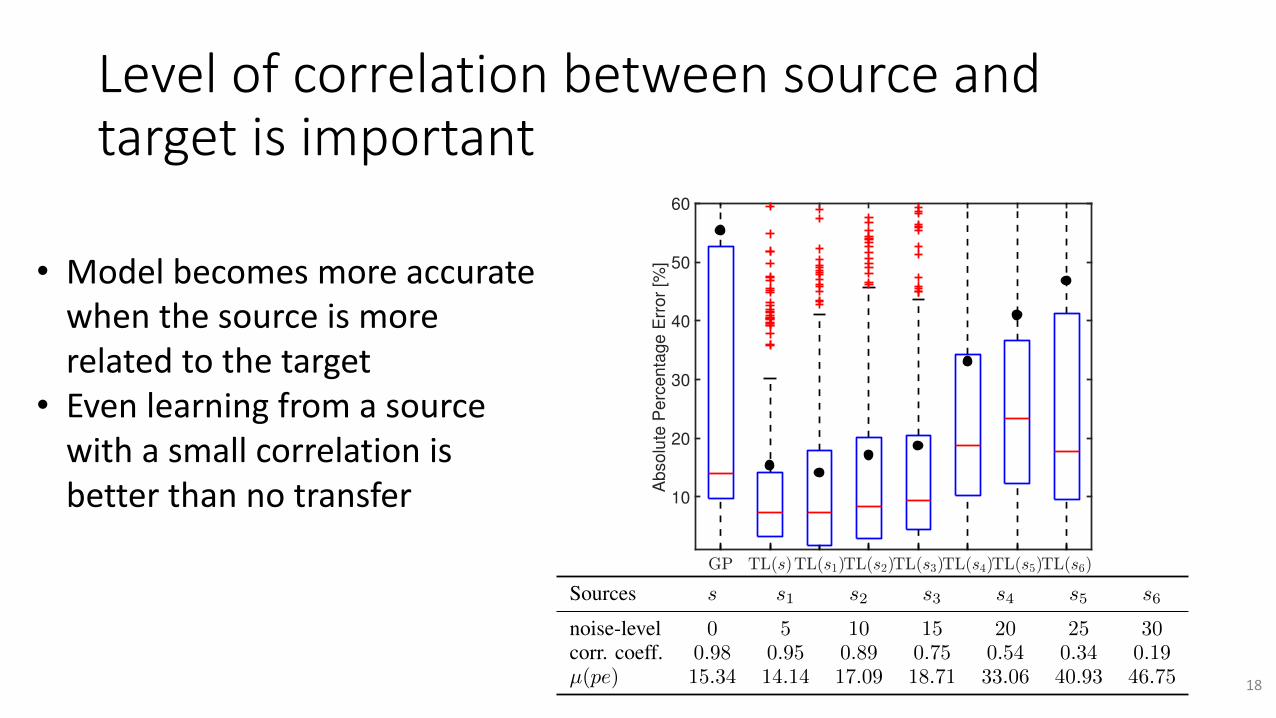
Levelofcorrelationbetweensourceandtargetisimportant

10

20

30

40

50

60

Ab

solu

te P

erc

en

tag

e E

rro

r [%

]

Sources s s1 s2 s3 s4 s5 s6

noise-level 0 5 10 15 20 25 30corr. coeff. 0.98 0.95 0.89 0.75 0.54 0.34 0.19µ(pe) 15.34 14.14 17.09 18.71 33.06 40.93 46.75

Fig. 6: Prediction accuracy of the model learned with samplesfrom different sources of different relatedness to the target.GP is the model without transfer learning.

the incoming stream and it is essentially a CPU intensiveapplication. RollingSort is a memory intensive system thatperforms rolling counts of incoming messages for identifyingtrending topics. SOL is a network intensive system, wherethe incoming messages will be routed through an multi-layer network. These are standard benchmarks that are widelyused in the community, e.g., research papers [14] as well asindustry benchmarks [18]. For more details about the internalarchitecture of these systems, we refer to the appendix [1].

The notion of source and target set depends on the subjectsystem. In CoBot, we again simulate the same navigation mis-sion in the default environment (source) and in a more difficultnoisy environment (target). For the three stream processingapplications, source and target represent different workloads,such that we transfer measurements from one workload forlearning a model for another workload. More specifically, wecontrol the workload using the maximum number of messageswhich we allow to enter the stream processing architecture. Forthe NoSQL application, we analyze two different transfers:First, we use as source a query on a database with 10 millionrecords and as target the same query on a database with 20million records, representing a more expensive environment tosample from. Second, we use as source a query on 20 millionrecords on one cluster and as target a query on the same datasetrun on a different cluster, representing hardware changes.Overall, our subjects cover different kinds of applicationsand different kinds of transfer scenarios (changes in theenvironment, changes in the workload, changes in the dataset,and changes in the hardware).

Experimental setup: As independent variables, we sys-tematically vary the size of the learning sets from both sourceand target environment in each subject system. We samplebetween 0 and 100 % of all configurations in the sourceenvironment and between 1 and 10 % of all configurationsin the target environment.

As dependent variable, we measure learning time and

TABLE I: Overview of our experimental datasets. “Size”column indicates the the number of measurements in thedatasets and “Testbed” refer to the infrastructure where themeasurements are taken and their details are in the appendix.

Dataset Parameters Size Testbed

1 CoBot(4D)

1-odom miscalibration,2-odom noise,3-num particles,4-num refinement

56585 C9

2 wc(6D)1-spouts, 2-max spout,3-spout wait, 4-splitters,5-counters, 6-netty min wait

2880 C1

3 sol(6D)1-spouts, 2-max spout,3-top level, 4-netty min wait,5-message size, 6-bolts

2866 C2

4 rs(6D)1-spouts, 2-max spout,3-sorters, 4-emit freq,5-chunk size, 6-message size

3840 C3

5

6

cass-10

cass-20

1-trickle fsync, 2-auto snapshot,3-con. reads, 4-con. writes5-file cache size in mb6-con. compactors

1024 C6x,C6y

prediction accuracy of the learned model. For each subjectsystem, we measure a large number of random configurationsas the evaluation set, independently from configurations sam-pled for learning, and compare the predictions of the learnedmodel f̂ to the actual measurements of the configurations inthe evaluation set D

o

. We compute the absolute percentageerror (APE) for each configuration x in the evaluation set|f̂(x)�f(x)|

f(x) ⇥ 100 and report the average to characterizeaccuracy of the prediction model. Ideally, we would use thewhole configuration space as evaluation set (D

o

= X), but themeasurement effort would be prohibitively high for most real-world systems [20], [31]; hence we use large random samples(cf. size column in Table I).

The measured and predicted metric depends on the subjectsystem: For the CoBot system, we measure average CPU usageduring the same mission of navigating along a corridor as inour case study; we use the average of three simulation runsfor each configuration. For the stream processing and NoSQLexperiments, we measure average response time (latency) overa window of 8 and 10 minutes respectively. Also, after eachsample collection, the experimental testbed was cleaned whichrequired several minutes for the Storm measurements andaround 1 hour (for offloading and cleaning the database) forthe Cassandra measurements. We sample the given number ofconfigurations in source and target randomly and report aver-age results and standard deviations of accuracy and learningtime over 3 repetitions.

Results: We show results of our experiments in Figure 7.The 2D plot shows average errors across all subject systems.The results in which the set of source samples D

s

is empty rep-resents the baseline case without transfer learning. In Figure 8,we additionally show a specific slice through our accuracyresults, in which we only vary the number of samples from thesource (and only for 4 subject systems to produce a reasonablyclear plot), but keep the number of samples from the target ata constant 1 %. Although the results differ significantly amongsubject systems (not surprising, given different relatedness ofsource and target) the overall trends are consistent.

First, our results show that transfer learning can achievehigh prediction accuracy with only few samples from the target

• Modelbecomesmoreaccuratewhenthesourceismorerelatedtothetarget

• Evenlearningfromasourcewithasmallcorrelationisbetterthannotransfer

18

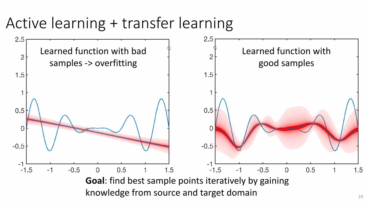
Activelearning+transferlearning

Learnedfunctionwithbadsamples->overfitting

Goal:findbestsamplepointsiterativelybygainingknowledgefromsourceandtargetdomain

Learnedfunctionwithgoodsamples

19

Conclusion:Ourcost-awaretransferlearning

• Improvesthemodelaccuracyuptoseveralordersofmagnitude• Isabletotrade-offbetweendifferentnumberofsamplesfromsourceandtargetenablingacost-awaremodel• Imposesanacceptablemodelbuildingandevaluationcostmakingappropriateforapplicationintheroboticsdomain

20