Clausius-Clapeyron equation

Masatsugu Sei Suzuki

Department of Physics, SUNY at Binghamton

(Date: November 27, 2017)

The Clausius–Clapeyron relation, named after Rudolf Clausius and Benoît Paul Émile

Clapeyron, is a way of characterizing a discontinuous phase transition between two phases of matter of a single constituent. On a pressure–temperature (P–T) diagram, the line separating the two phases is known as the coexistence curve. The Clausius–Clapeyron relation gives the slope of the tangents to this curve. Mathematically,

VT

L

V

S

dT

dP

The derivation of this equation was a remarkable early accomplishment of thermodynamics. Both sides of this equation are easily determined experimentally. The equation has been verified to high precision. 1. Phase diagram of water

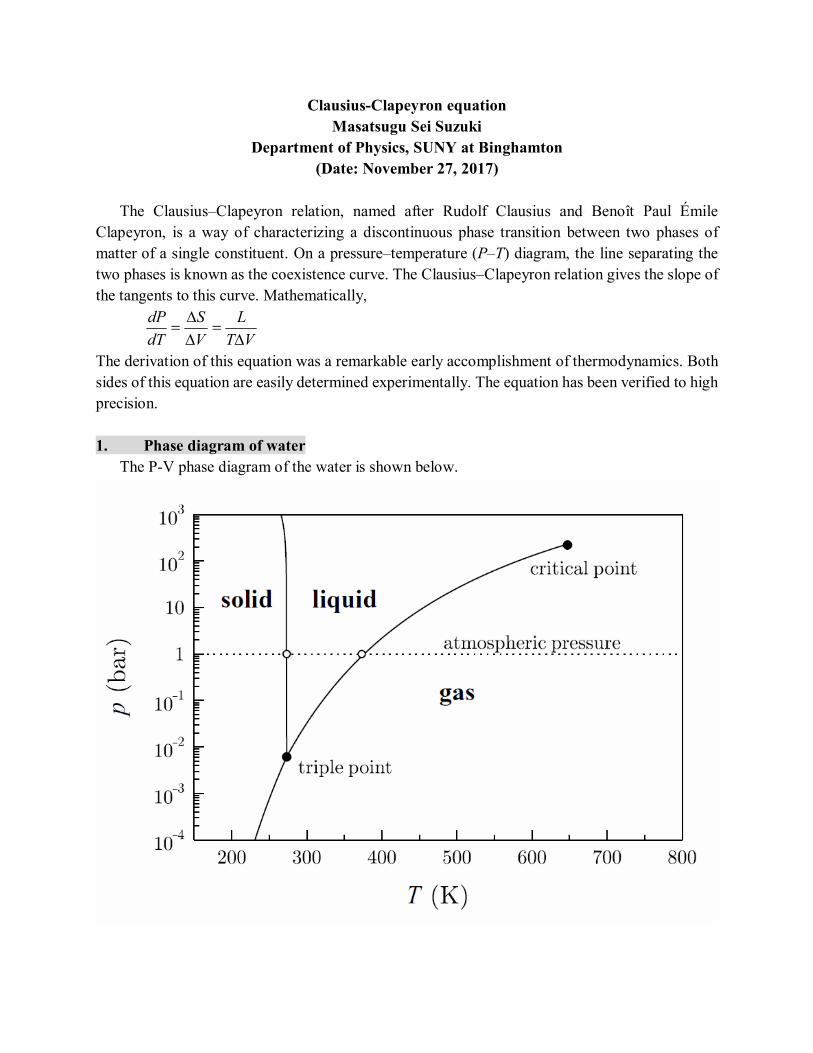
The P-V phase diagram of the water is shown below.

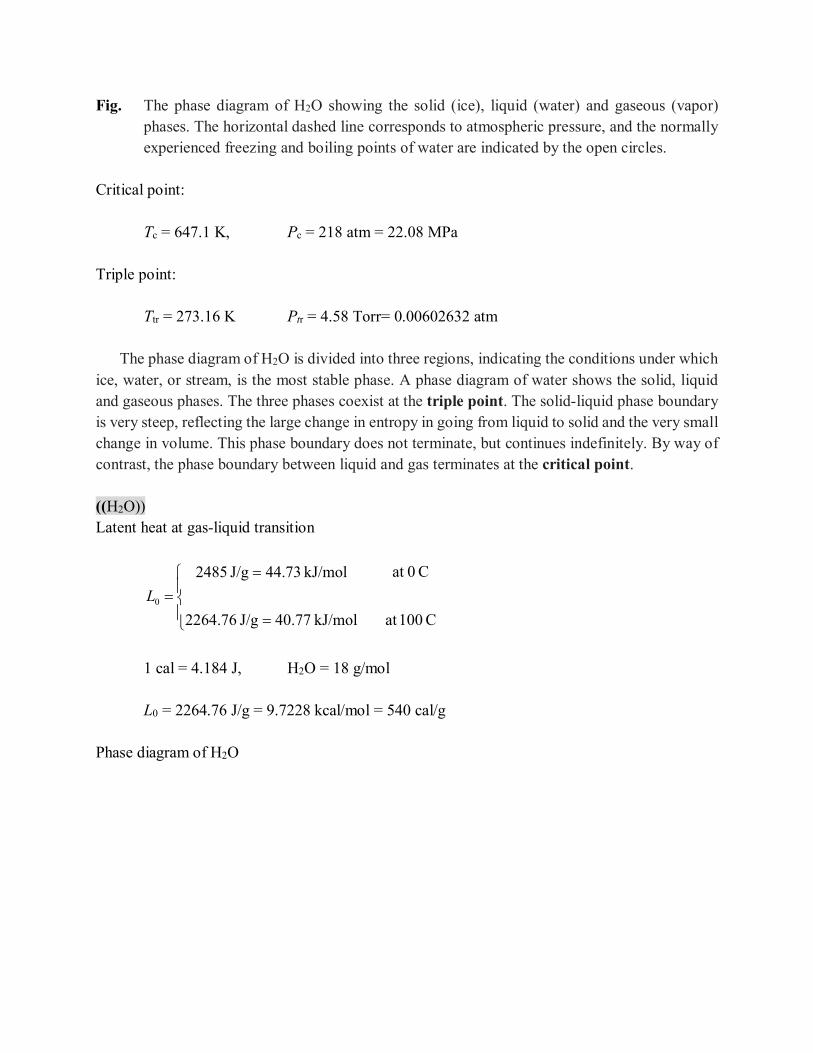
Fig. The phase diagram of H2O showing the solid (ice), liquid (water) and gaseous (vapor) phases. The horizontal dashed line corresponds to atmospheric pressure, and the normally experienced freezing and boiling points of water are indicated by the open circles.

Critical point:

Tc = 647.1 K, Pc = 218 atm = 22.08 MPa Triple point:

Ttr = 273.16 K Ptr = 4.58 Torr= 0.00602632 atm

The phase diagram of H2O is divided into three regions, indicating the conditions under which ice, water, or stream, is the most stable phase. A phase diagram of water shows the solid, liquid and gaseous phases. The three phases coexist at the triple point. The solid-liquid phase boundary is very steep, reflecting the large change in entropy in going from liquid to solid and the very small change in volume. This phase boundary does not terminate, but continues indefinitely. By way of contrast, the phase boundary between liquid and gas terminates at the critical point. ((H2O)) Latent heat at gas-liquid transition

kJ/mol .7704J/g 76.2264

kJ/mol 73.44J/g 2485

0L

C 100at

C 0at

1 cal = 4.184 J, H2O = 18 g/mol

L0 = 2264.76 J/g = 9.7228 kcal/mol = 540 cal/g

Phase diagram of H2O

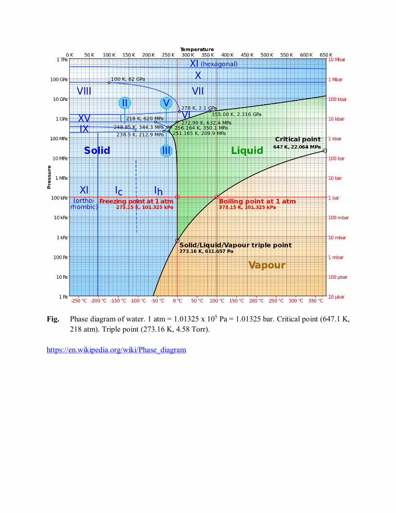
Fig. Phase diagram of water. 1 atm = 1.01325 x 105 Pa = 1.01325 bar. Critical point (647.1 K,

218 atm). Triple point (273.16 K, 4.58 Torr). https://en.wikipedia.org/wiki/Phase_diagram

Table: The vapor pressure and molar latent heat for the solid-gas transformation (first three entries) and the liquid-gas transformation (remaining entries). Data from Keenan et al. (1978) and Lide (1994).

2. Derivation of Clausius-Clapeyron equation from the Carnot cycle (Adkins)

P bar

T C

100 200 300

10 4

0.001

0.010

0.100

1

10

100

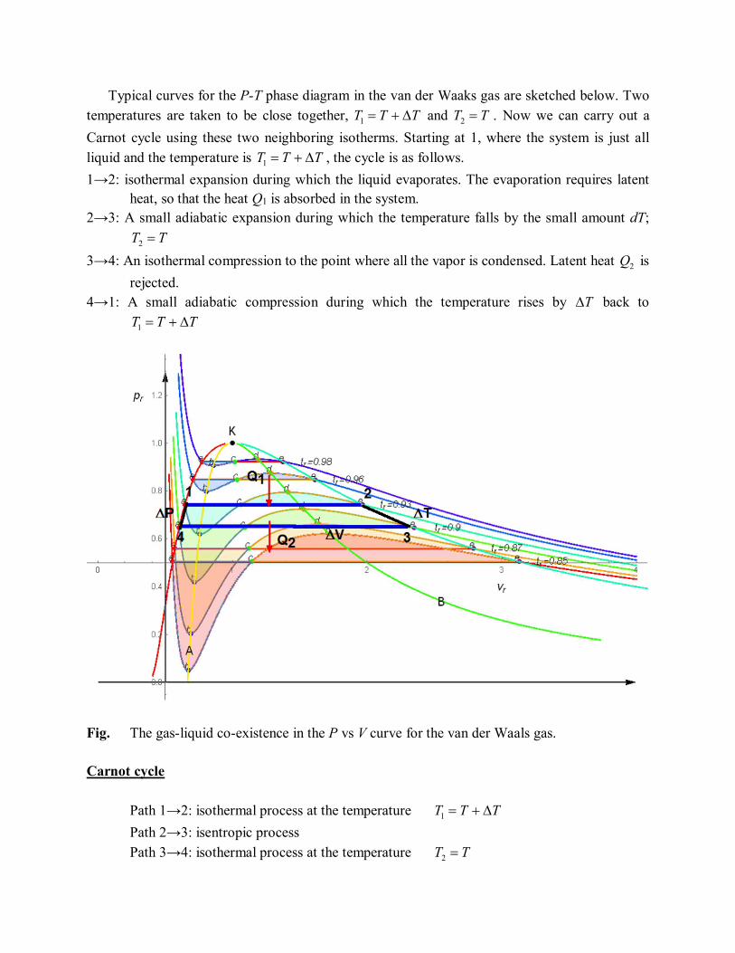
Typical curves for the P-T phase diagram in the van der Waaks gas are sketched below. Two

temperatures are taken to be close together, TTT 1 and TT 2 . Now we can carry out a

Carnot cycle using these two neighboring isotherms. Starting at 1, where the system is just all

liquid and the temperature is TTT 1 , the cycle is as follows.

1→2: isothermal expansion during which the liquid evaporates. The evaporation requires latent heat, so that the heat Q1 is absorbed in the system.

2→3: A small adiabatic expansion during which the temperature falls by the small amount dT;

TT 2

3→4: An isothermal compression to the point where all the vapor is condensed. Latent heat 2Q is

rejected. 4→1: A small adiabatic compression during which the temperature rises by T back to

TTT 1

Fig. The gas-liquid co-existence in the P vs V curve for the van der Waals gas. Carnot cycle

Path 1→2: isothermal process at the temperature TTT 1

Path 2→3: isentropic process

Path 3→4: isothermal process at the temperature TT 2

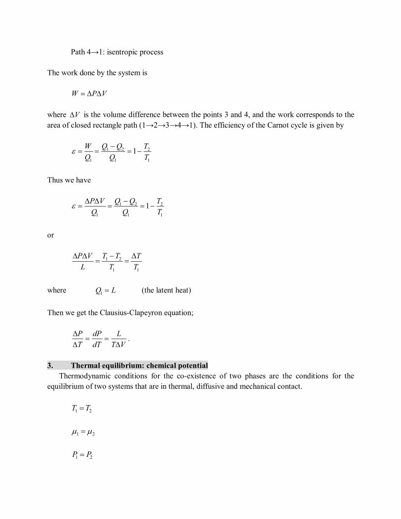
Path 4→1: isentropic process The work done by the system is

VPW where V is the volume difference between the points 3 and 4, and the work corresponds to the area of closed rectangle path (1→2→3→4→1). The efficiency of the Carnot cycle is given by

1

2

1

21

1

1T

T

Q

QQ

Q

W

Thus we have

1

2

1

21

1

1T

T

Q

QQ

Q

VP

or

11

21

T

T

T

TT

L

VP

where LQ 1 (the latent heat)

Then we get the Clausius-Clapeyron equation;

VT

L

dT

dP

T

P

.

3. Thermal equilibrium: chemical potential

Thermodynamic conditions for the co-existence of two phases are the conditions for the equilibrium of two systems that are in thermal, diffusive and mechanical contact.

21 TT

21

21 PP

For liquid and gas

TTT gl , gl , PPP gl .

The chemical potential:

),(),( TPTP gl

At a general point in the P-T plane the two phases do not co-exist.

If gl , the liquid phase alone is stable.

If lg , the gas phase alone is stable.

((Note)) Metastable phases may occur, by supercooling or superheating. 4. Derivative of the co-existence curve, P vs T:

),(),( 0000 TPTP lg

This is a condition of co-existence. We start with an equation

),(),( 0000 dTTdPPdTTdPP lg

We make a series expansion

dTT

dPP

TPdTT

dPP

TPP

l

T

ll

P

g

T

g

g

),(),( 0000

In the limit as dP and dT approach zero,

dTT

dPP

dTT

dPP P

l

T

l

P

g

T

g

This may be rearranged to give

T

l

T

g

P

g

P

l

PP

TT

dT

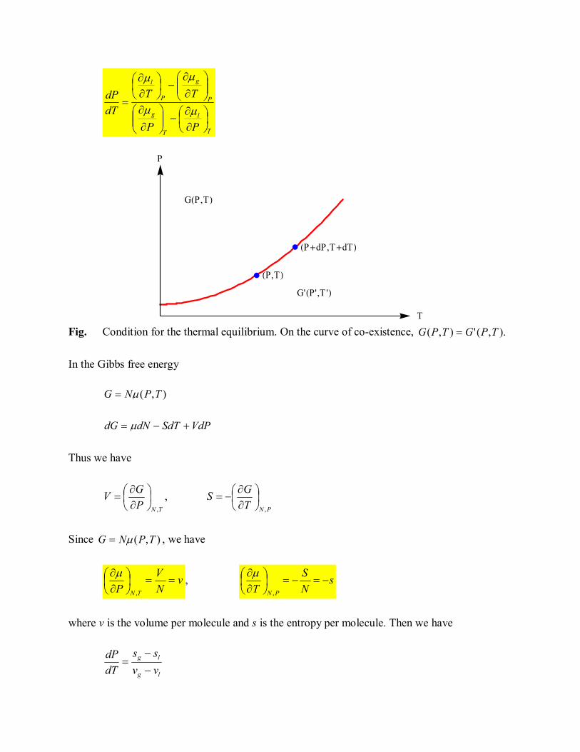
dP

Fig. Condition for the thermal equilibrium. On the curve of co-existence, ).,('),( TPGTPG

In the Gibbs free energy

),( TPNG

VdPSdTdNdG

Thus we have

TNP

GV

,

, PNT

GS

,

Since ),( TPNG , we have

vN

V

P TN

,

, s

N

S

T PN

,

where v is the volume per molecule and s is the entropy per molecule. Then we have

lg

lg

vv

ss

dT

dP

P

T

GHP,TL

G'HP',T 'L

HP+dP,T+dTL

HP,TL

5. Derivation of Clausius-Clapeyron equation from Gibbs-Duhem relation

The Gibbs energy:

VdPSdTdNdG

Since NG , this equation can be rewritten as

VdPSdTdNNddNdG

or

vdPsdTdPN

VdT

N

Sd (Gibbs-Duhem relation)

where S

sN

, V

vN

.

Suppose that two phases 1 and 2 are in-contact and at equilibrium with each other. The chemical potentials are related by

21 .

Furthermore, along the co-existence curve,

21 dd

Here we use the Gibbs-Duhem relation,

vdPsdTd

to obtain

dPvdTsdPvdTs 2211

or

12

12

vv

ss

dT

dP

(Clausius-Clapeyron equation)

6. Clausius-Clapeyron equation

' ( )g ld Q T s s l

l : latent heat of vaporization/molecule

lg vvv

Thus we have the Clausius-Clapeyron equation,

dP l

dT T v

Two approximations:

(a) lg vv

g

g

glgN

Vvvvv

(b)

TkNPV Bgg (ideal gas law)

or

TkPv Bg

Using these two approximations, we have

2g g B

dP l l lP lP

dT T v Tv TPv k T

Suppose that the latent heat l is independent of T;

2B

dP l dT

P k T

or

lnB

lP

k T +constant

or

0( ) exp( )B

lP T P

k T

where L0 is the latent heat of vaporization of one molecule. If 0L refers instead to one mole, then

A

B A

lN L

k N R

0( ) exp( )L

P T PRT

.

where

R = 8.3144598 [J/(K mol)]. AL lN .

L = 2256 x 18.01528 = 40.642 (kJ/mol): latent heat of vaporization/mol for water: 7. Phase diagram of H2O and Clausius-Clapeyron equation

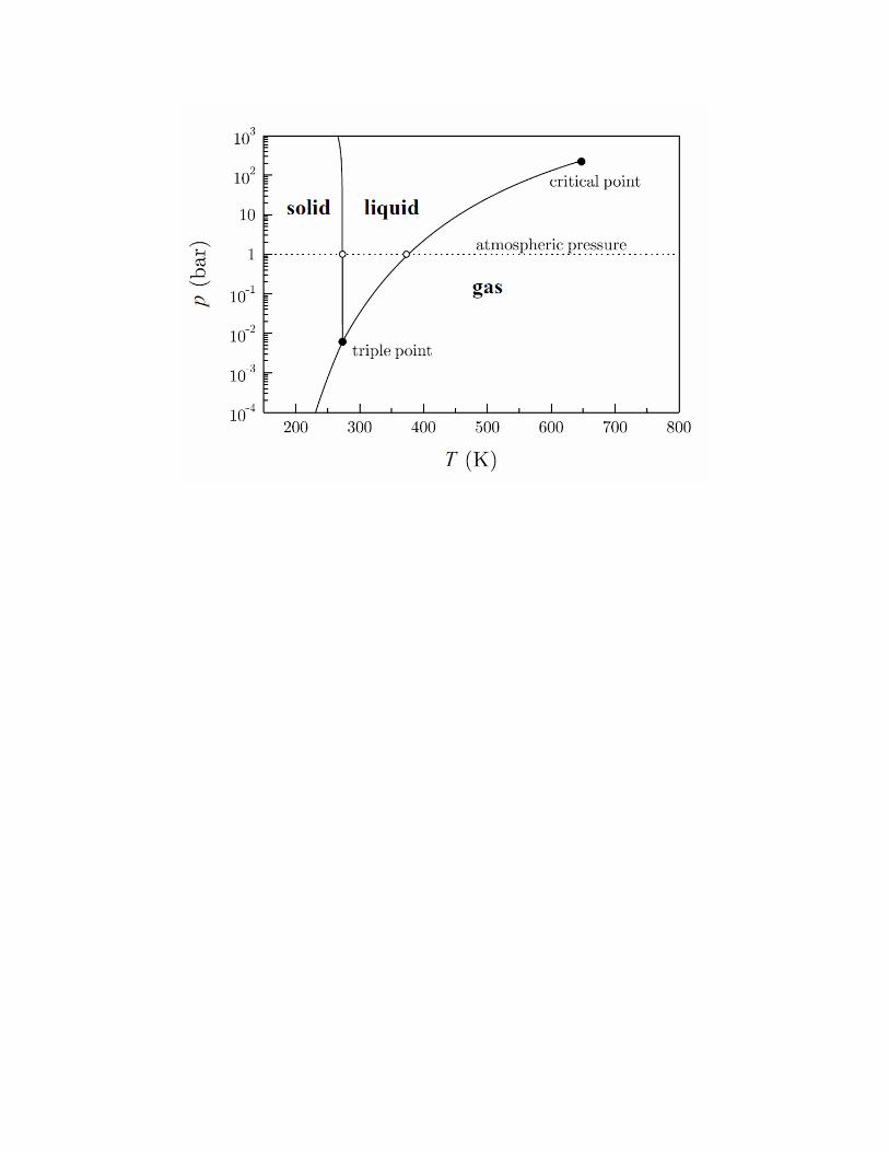
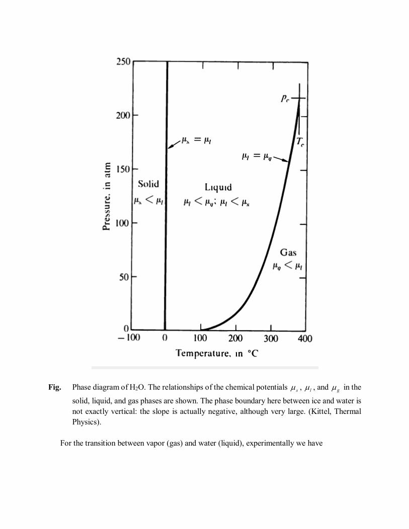
Fig. Phase diagram of H2O. The relationships of the chemical potentials s , l , and g in the

solid, liquid, and gas phases are shown. The phase boundary here between ice and water is not exactly vertical: the slope is actually negative, although very large. (Kittel, Thermal Physics).

For the transition between vapor (gas) and water (liquid), experimentally we have

0

lg

lg

vv

ss

dT

dP (see the phase diagram of water)

Since lg vv , we get

lg ss

For the transition between ice (solid) and water (liquid), experimentally we have

0

ls

ls

vv

ss

dT

dP (see the phase diagram of water)

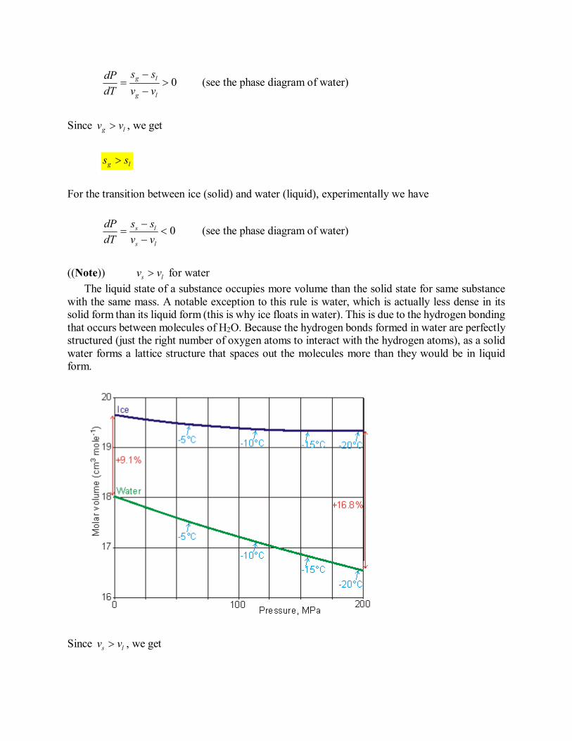
((Note)) ls vv for water

The liquid state of a substance occupies more volume than the solid state for same substance with the same mass. A notable exception to this rule is water, which is actually less dense in its solid form than its liquid form (this is why ice floats in water). This is due to the hydrogen bonding that occurs between molecules of H2O. Because the hydrogen bonds formed in water are perfectly structured (just the right number of oxygen atoms to interact with the hydrogen atoms), as a solid water forms a lattice structure that spaces out the molecules more than they would be in liquid form.

Since ls vv , we get

sl ss

In summary, we have

slg sss

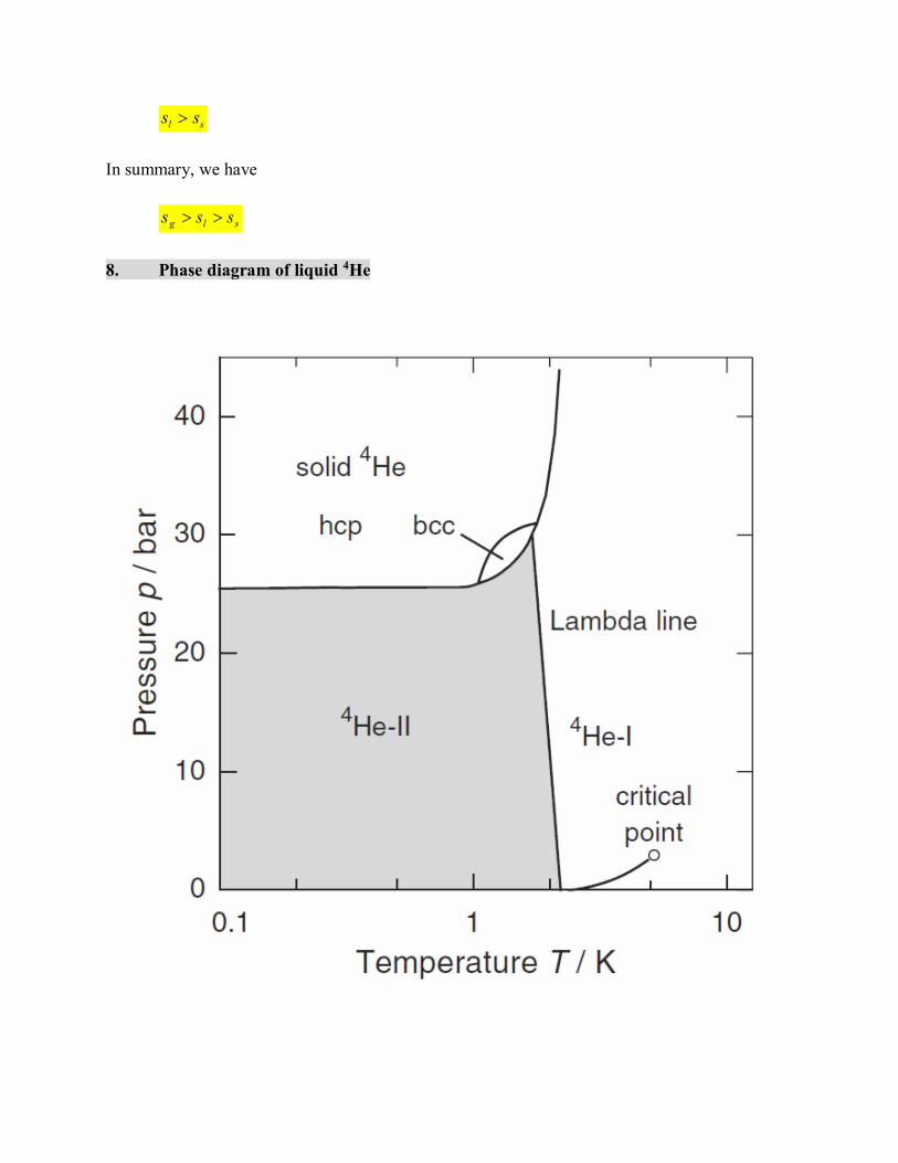
8. Phase diagram of liquid 4He

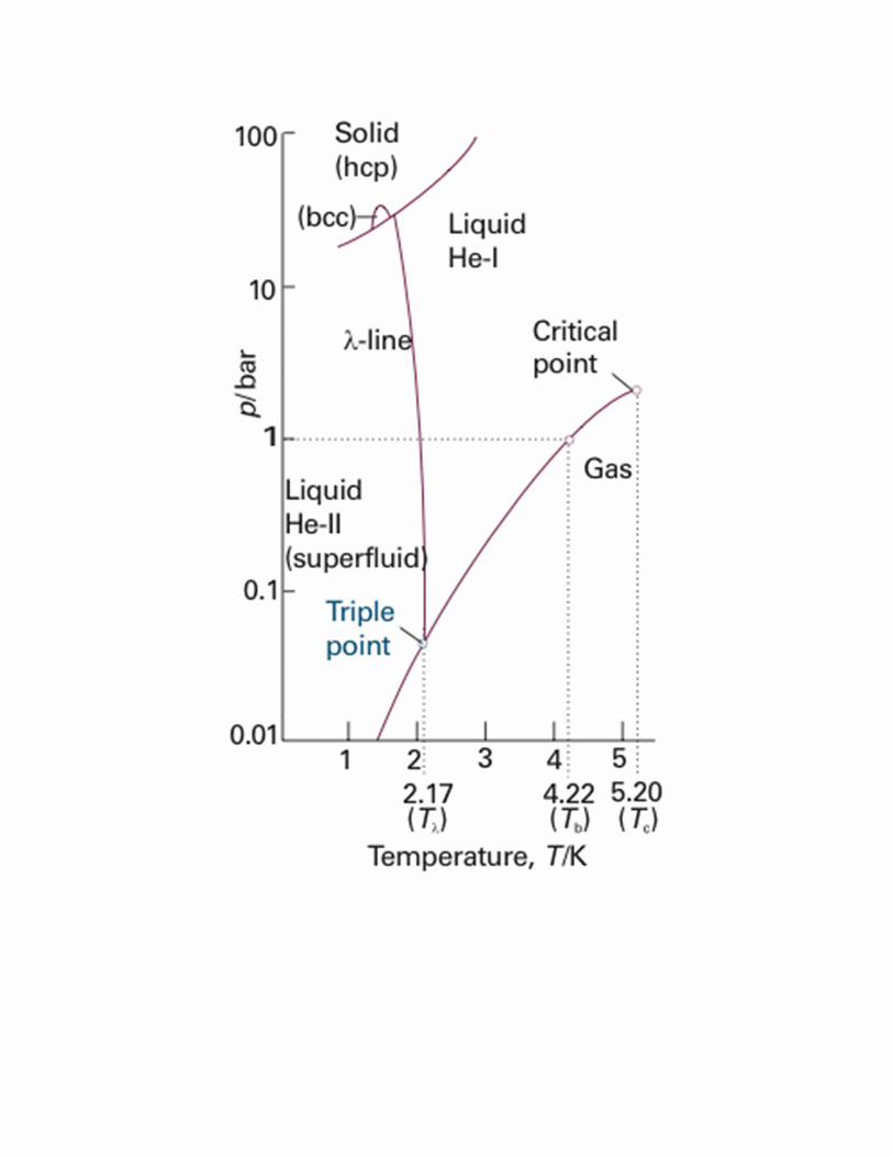
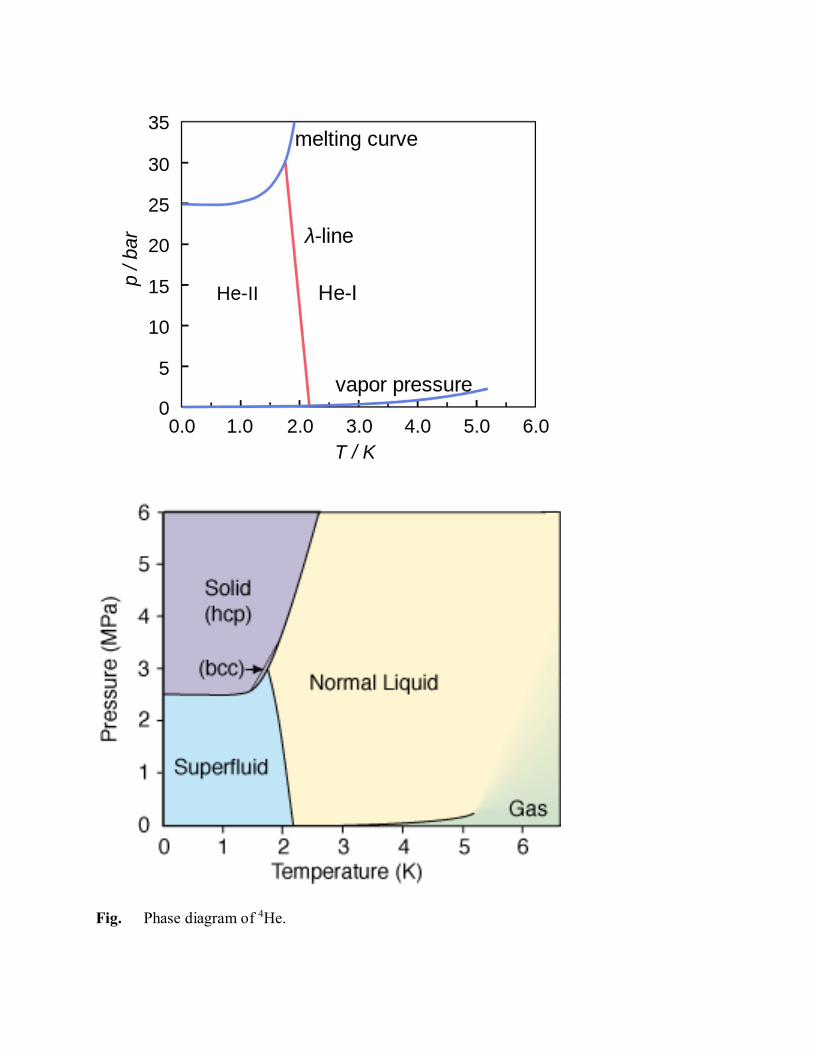
Fig. Phase diagram of 4He.

The Clausius-Clayperon equation is also applied to the solid-liquid transition

sl

sl

vv

ss

dT

dP

In the phase diagram of 4He, the liquid-solid co-existence curve is closely horizontal for T<1.4 K.

sl ss

Note that the entropy of a normal liquid is considerably higher than that of a normal solid.

At low temperatures (T ≈ 0.8 K) the melting curve exhibits a shallow minimum, which is not deep enough to be visible on the scale of the phase diagram of 4He,. Using the Clausius Clapeyron equation curve, we can draw conclusions about the entropies of liquid and solid 4He. Since ls vv ,

we have

sl ss

which means that the entropy of the solid phase is larger than the entropy of the liquid phase. In other words, the disorder in the solid is larger than in the liquid. The entropy of solid and liquid 4He is determined by thermal excitations in this temperature range. It turns out that solid 4He has a slightly higher phonon heat capacity than liquid 4He, because of the low transverse sound velocity in solid 4He. Therefore, at low temperatures the entropy of solid 4He is larger than that of liquid 4He. 9. Phase diagram of liquid 3He

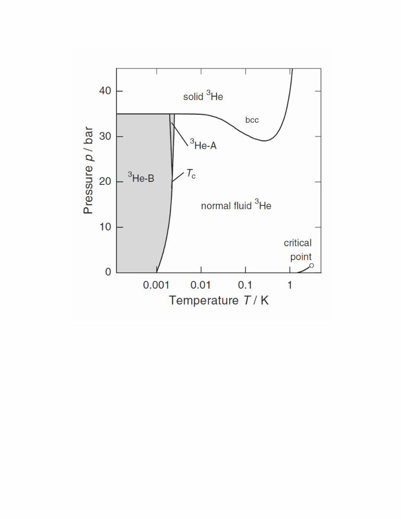
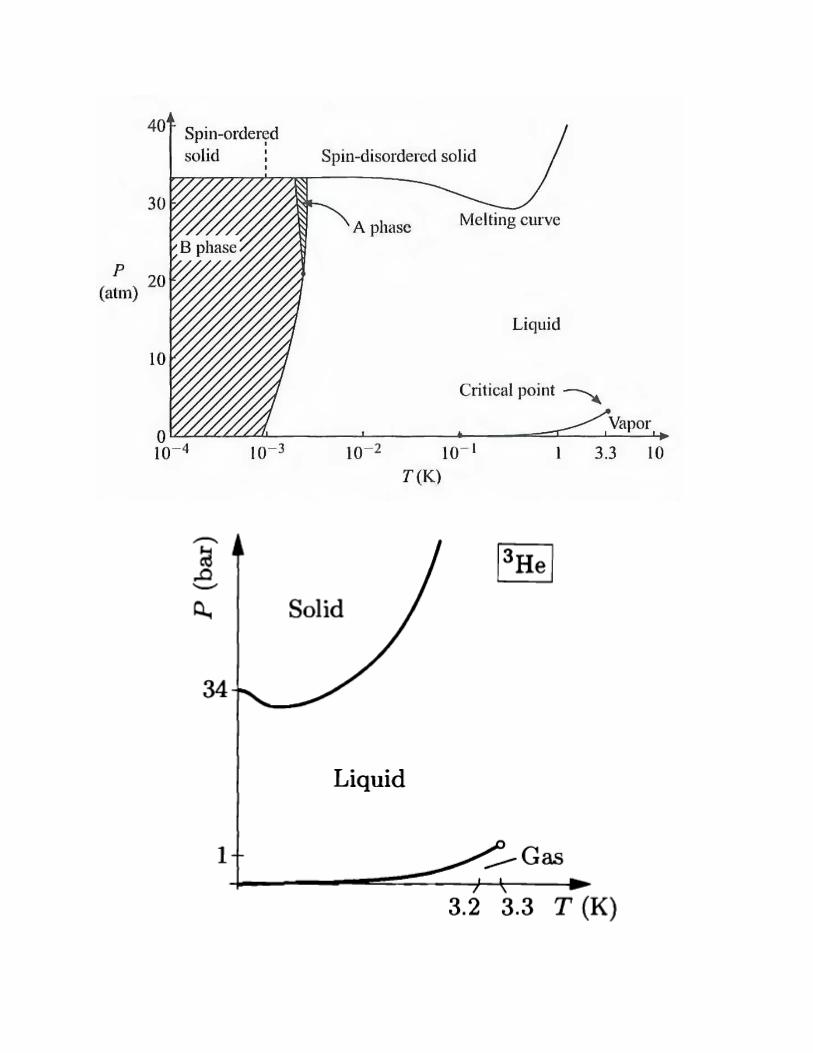
Fig. Phase diagram of 3He.

Fig. Phase diagram of 3He. The Clausius-Clapeyron equation,

0

sl

sl

vv

ss

dT

dP

Since sl vv , we have

sl ss .

The entropy of liquid is less than the entropy of the solid.

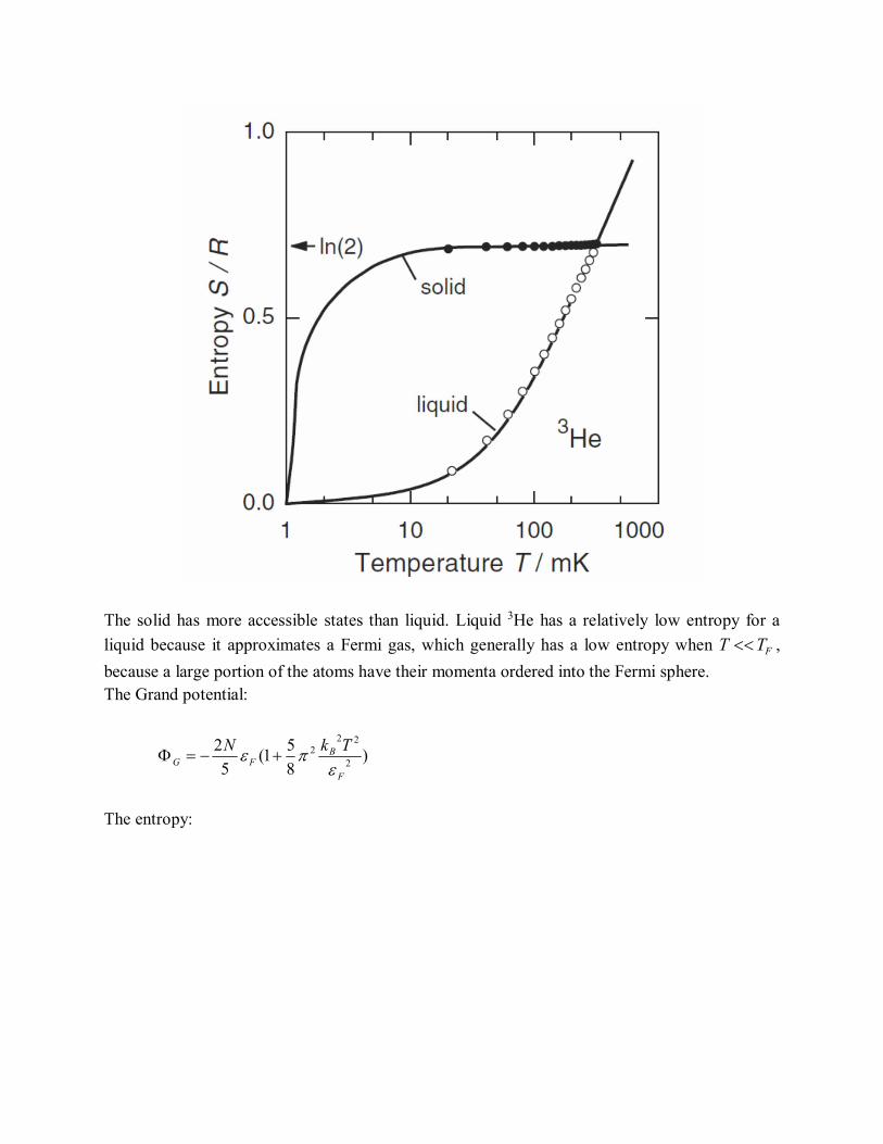
The solid has more accessible states than liquid. Liquid 3He has a relatively low entropy for a

liquid because it approximates a Fermi gas, which generally has a low entropy when FTT ,

because a large portion of the atoms have their momenta ordered into the Fermi sphere. The Grand potential:

)8

51(

5

22

222

F

BFG

TkN

The entropy:

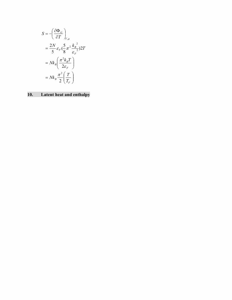
F

B

F

BB

F

BF

V

G

T

TNk

TkNk

TkN

TS

2

2

2)8

5(

5

2

2

2

2

22

,

10. Latent heat and enthalpy

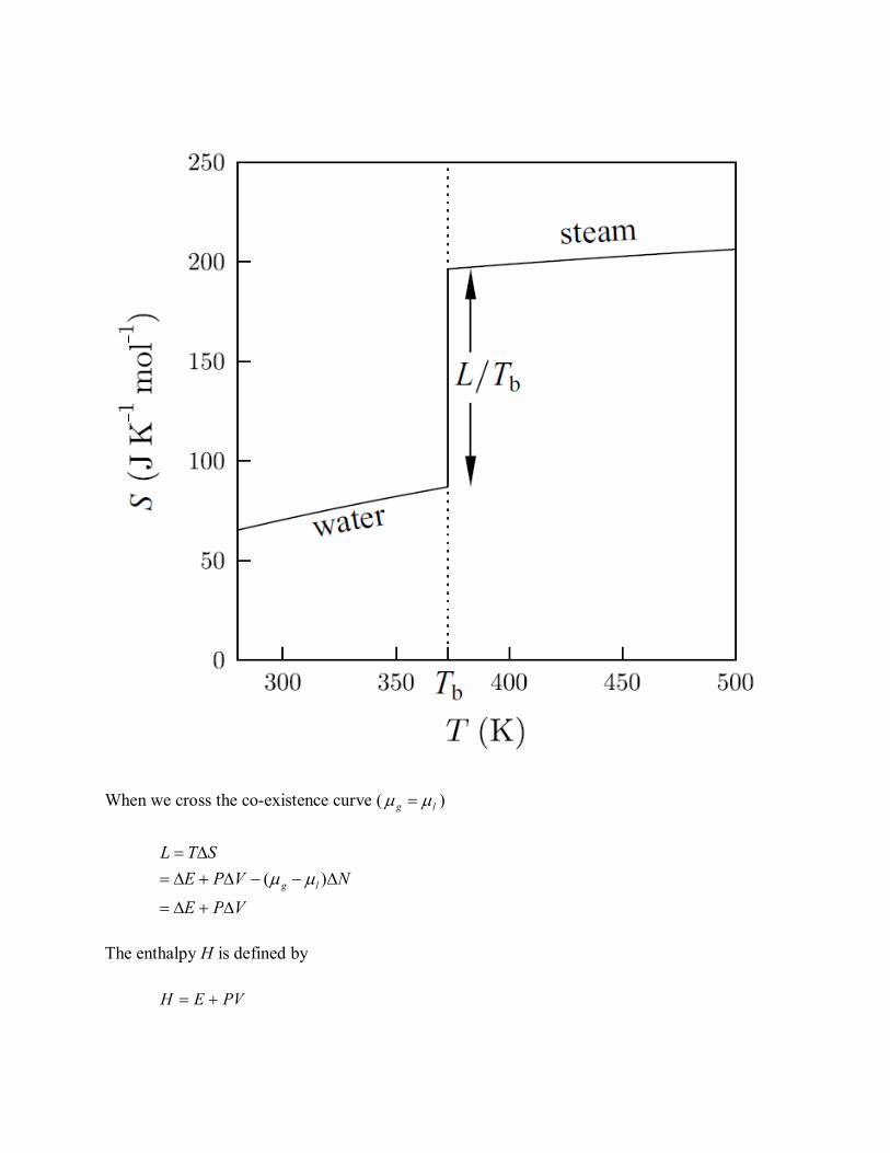
When we cross the co-existence curve ( lg )

VPE

NVPE

STL

lg

)(

The enthalpy H is defined by

PVEH

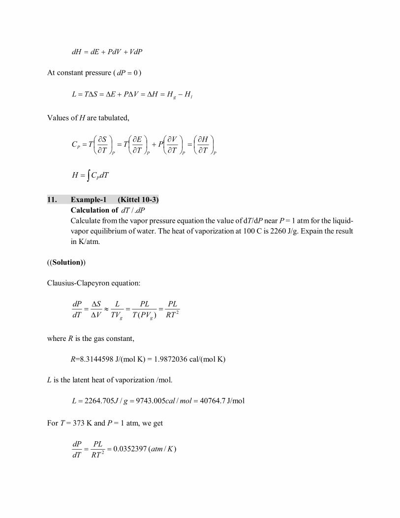
VdPPdVdEdH At constant pressure ( 0dP )

lg HHHVPESTL

Values of H are tabulated,

PPPP

PT

H

T

VP

T

ET

T

STC

dTCH P

11. Example-1 (Kittel 10-3)

Calculation of dPdT ./

Calculate from the vapor pressure equation the value of dT/dP near P = 1 atm for the liquid-vapor equilibrium of water. The heat of vaporization at 100 C is 2260 J/g. Expain the result in K/atm.

((Solution)) Clausius-Clapeyron equation:

2)( RT

PL

PVT

PL

TV

L

V

S

dT

dP

gg

where R is the gas constant,

R=8.3144598 J/(mol K) = 1.9872036 cal/(mol K) L is the latent heat of vaporization /mol.

7.40764/005.9743/705.2264 molcalgJL J/mol

For T = 373 K and P = 1 atm, we get

)/( 0352397.02

KatmRT

PL

dT

dP

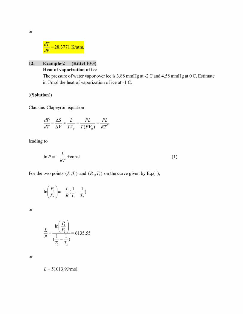
or

dP

dT28.3771 K/atm.

12. Example-2 (Kittel 10-3)

Heat of vaporization of ice

The pressure of water vapor over ice is 3.88 mmHg at -2 C and 4.58 mmHg at 0 C. Estimate in J/mol the heat of vaporization of ice at -1 C.

((Solution)) Clausius-Clapeyron equation

2)( RT

PL

PVT

PL

TV

L

V

S

dT

dP

gg

leading to

RT

LP ln +const (1)

For the two points ),( 11 TP and ),( 212 TP on the curve given by Eq.(1),

)11

(ln212

1

TTR

L

P

P

or

)11

(

ln

22

2

1

TT

P

P

R

L

= 6135.55

or

J/mol9.51013L

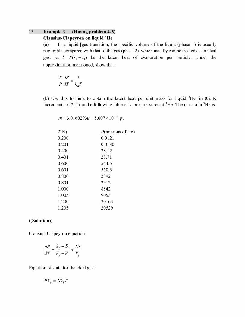
13 Example 3 (Huang problem 4-5)

Clausius-Clapeyron on liquid 3He

(a) In a liquid-[gas transition, the specific volume of the liquid (phase 1) is usually negligible compared with that of the gas (phase 2), which usually can be treated as an ideal

gas. let )( 12 ssTl be the latent heat of evaporation per particle. Under the

approximation mentioned, show that

Tk

l

dT

dP

P

T

B

(b) Use this formula to obtain the latent heat per unit mass for liquid 3He, in 0.2 K increments of T, from the following table of vapor pressures of 3He. The mass of a 3He is

gum 10007.50160293.3 24 .

T(K) P(microns of Hg) 0.200 0.0121 0.201 0.0130 0.400 28.12 0.401 28.71 0.600 544.5 0.601 550.3 0.800 2892 0.801 2912 1.000 8842 1.005 9053 1.200 20163 1.205 20529

((Solution)) Clausius-Clapeyron equation

glg

lg

V

S

VV

SS

dT

dP

Equation of state for the ideal gas:

TNkPV Bg

Thus we get

TNk

SP

PV

SP

dT

dP

Bg

or

Tk

l

TNk

L

Nk

S

dT

dP

P

T

BBB

or

2

1

T

dT

k

ldP

P B

, CTk

lP

B

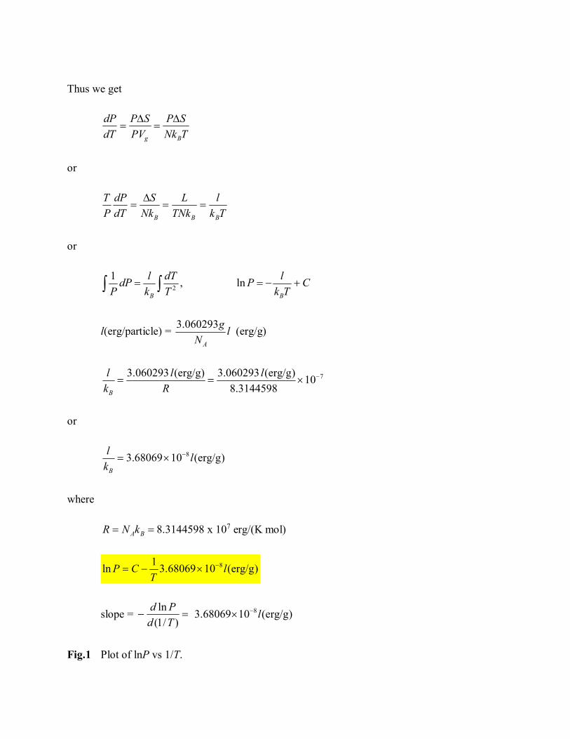
ln

l(erg/particle) = lN

g

A

060293.3 (erg/g)

710 8.3144598

)erg/g( 060293.3(erg/g) 060293.3 l

R

l

k

l

B

or

)erg/g(1068069.3 8 lk

l

B

where

BAkNR 8.3144598 x 107 erg/(K mol)

)erg/g(1068069.31

ln 8 lT

CP

slope = )/1(

ln

Td

Pd )erg/g(1068069.3 8 l

Fig.1 Plot of lnP vs 1/T.

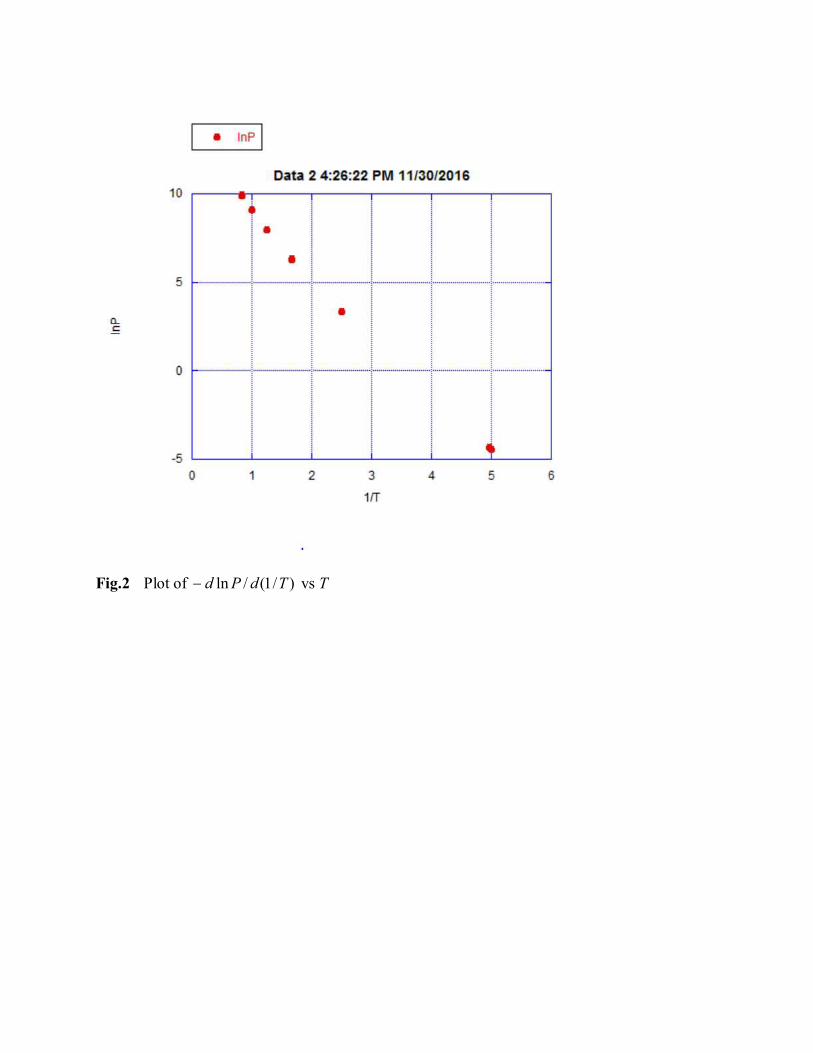
Fig.2 Plot of )/1(/ln TdPd vs T

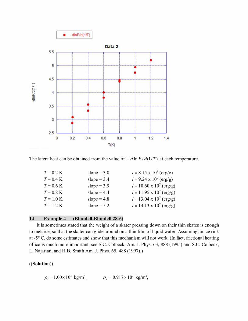
The latent heat can be obtained from the value of )/1(/ln TdPd at each temperature.

T = 0.2 K slope = 3.0 l 8.15 x 107 (erg/g) T = 0.4 K slope = 3.4 l 9.24 x 107 (erg/g) T = 0.6 K slope = 3.9 l 10.60 x 107 (erg/g) T = 0.8 K slope = 4.4 l 11.95 x 107 (erg/g) T = 1.0 K slope = 4.8 l 13.04 x 107 (erg/g) T = 1.2 K slope = 5.2 l 14.13 x 107 (erg/g)

14 Example 4 (Blundell-Blundell 28-6)

It is sometimes stated that the weight of a skater pressing down on their thin skates is enough to melt ice, so that the skater can glide around on a thin film of liquid water. Assuming an ice rink at -5° C, do some estimates and show that this mechanism will not work. (In fact, frictional heating of ice is much more important, see S.C. Colbeck, Am. J. Phys. 63, 888 (1995) and S.C. Colbeck, L. Najarian, and H.B. Smith Am. J. Phys. 65, 488 (1997).) ((Solution))

31000.1 l kg/m3, 310917.0 s kg/m3,

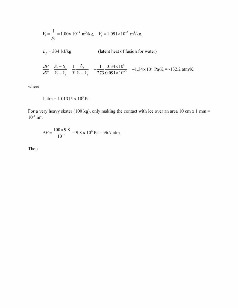
31000.11

l

lV

m3/kg, 310091.1 sV m3/kg,

334fL kJ/kg (latent heat of fusion for water)

73

5

1034.110091.0

1034.3

273

11

sl

f

sl

sl

VV

L

TVV

SS

dT

dP Pa/K = -132.2 atm/K.

where

1 atm = 1.01315 x 105 Pa. For a very heavy skater (100 kg), only making the contact with ice over an area 10 cm x 1 mm = 10-4 m2.

410

8.9100

P = 9.8 x 106 Pa = 96.7 atm

Then

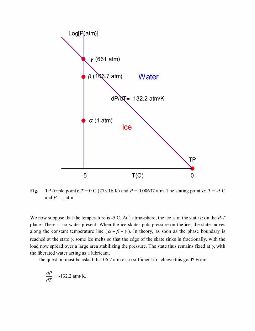
Fig. TP (triple point): T = 0 C (273.16 K) and P = 0.00637 atm. The stating point : T = -5 C and P = 1 atm.

We now suppose that the temperature is -5 C. At 1 atmosphere, the ice is in the state on the P-T plane. There is no water present. When the ice skater puts pressure on the ice, the state moves along the constant temperature line ( ). In theory, as soon as the phase boundary is

reached at the state , some ice melts so that the edge of the skate sinks in fractionally, with the

load now spread over a large area stabilizing the pressure. The state thus remains fixed at , with the liberated water acting as a lubricant.

The question must be asked: Is 106.7 atm or so sufficient to achieve this goal? From

dT

dP -132.2 atm/K.

TP

Log P atm

T C 05

1 atm

106.7 atm

661 atm

Ice

Water

dP dT 132.2 atm K

So a pressure increase of (132.2 atm/K) x 5 K = 661 atm would be required to go to from to . Thus this explanation for the success of the skater appears inadequate. ((Note)) Thermal conductivity:

3.2ice W/(m K)

56.0water W/(m K)

The gas constant:

3145.8R J/(K mol) Latent heat of fusion:

334fL kJ/kg

Latent heat of vaporization:

2260vL kJ/ kg

The density

31000.1 water kg/m3.

310917.0 ice kg/m3.

3100951.011

waterice m3/kg

REFERENCES

C. Kittel and H. Kroemer, Thermal Physics, second edition (W.H. Freeman and Company, 1980). C.J. Adkins, An Introduction to Thermal Physics (Cambridge 1987). C.J. Adkins, Equilibrium Thermodynamics, third edition (Cambridge, 1983). K. Huang, Introduction to Statistical Physics, second edition (CRC Press, 2010).

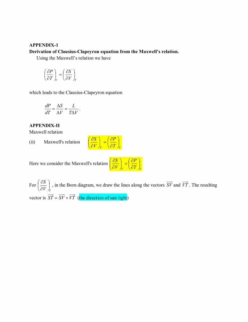
APPENDIX-1

Derivation of Clausius-Clapeyron equation from the Maxwell’s relation.

Using the Maxwell’s relation we have

TV V

S

T

P

which leads to the Clausius-Clapeyron equation

VT

L

V

S

dT

dP

.

APPENDIX-II

Maxwell relation

(ii) Maxwell's relation VT T

P

V

S

Here we consider the Maxwell's relation VT T

P

V

S

For TV

S

, in the Born diagram, we draw the lines along the vectors SV and VT . The resulting

vector is VTSVST (the direction of sun light)

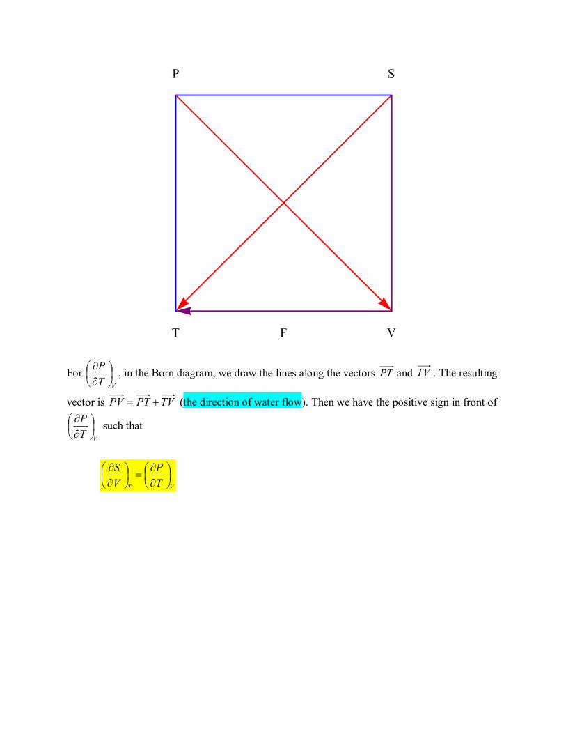
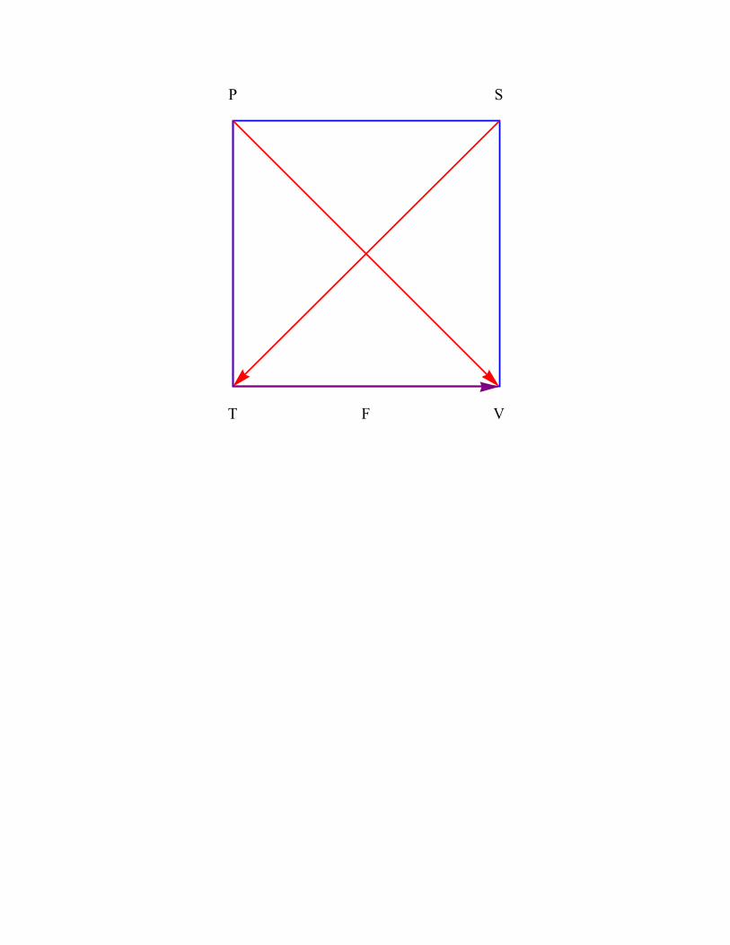
For VT

P

, in the Born diagram, we draw the lines along the vectors PT and TV . The resulting

vector is TVPTPV (the direction of water flow). Then we have the positive sign in front of

VT

P

such that

VT T

P

V

S

T V

P

F

S

T V

P

F

S