1994 ambient monitoring program manual - WA - DNR

76 Timber-Fish-Wildlife . TFW-AM9-94-001

AMBIENT MONITORING PROGRAM MANUAL

M ~ Stream Segment Identification o ~ Reference Point Survey D ~ Habitat Unit Survey U ~ Large Woody Debris Survey L ~ Saimonid Spawning Gravel Composition E ~ Stream Temperature Survey S ~ Quality Assurance

Edited by:

Dave Schuett-Hames Allen Pleus

Lyman Bullchild

Scott Hall

Northwest Indian Fisheries Commission

August 1994

· TIMBER-FISH-WILDLIFE

1994 AMBIENT MONITORING PROGRAM MANUAL

CONTENTS

The TFW Ambient Monitoring Program....... .......... .... Section 1

Stream Segment Identification Module.......... ............. Section 2

Reference Point Survey Module... ........ ............... ........ Section 3

Habitat 1(Jnit Survey Module........................................ Section Ll

Large Woody Debris Survey Module........................... Section 5

Salmonid Spawning Gravel Composition Module....... Section 6

Stream Temperature Module........................................ Section 7

-

Quality Assurance Module......................................... Section 8

(

THE TFW AMBIENT MONITORING PROGRAM

Contents

Acknowledgements .............................................. : ..................................................... 2

Introduction ................................................................................................................ 3

Goals of the Ambient Monitoring Stream Survey Project ............................................ 3

Ambient Monitoring Supports TFW and Watershed Analysis ..................................... 3

Organization of the TFW Ambient Monitoring Program ....... ...................................... 4

Products and Services Provided by the Ambient Monitoring Program ..... ................... 4

The Modular Structure of the Ambient Monitoring Program ....................................... 4

Uses ofTFW Ambient Monitoring Information ..................................................... ~ .... 5

Assessment of stream channel and habitat conditions................................................................ 5 Trend Monitoring...................................................................................................................... 6 Watershed Analysis..... ..... ..... .......... ..... ... ... ...... ... ... ... ... ... ... ... ....... ... ..... ........... ....... ..... ..... ... ...... 6 Estimating Habitat Carrying Capacity.. ........ ....... ........ ....... ..... ............... ......... ....... ............... .... 6

Training, Field Assistance and Quality Control .................................................... ....... 6

Data Processing and Outputs ...................................................................................... 7

For More Information About Participating in the Program .......................................... 7

References .................. ................................................................................................. 7

1994 TFW Ambient Monitoring Manual Introduction - I

L

r----......-----------------

Acknowledgements

The continued development of the TFW Ambient Monitoring project represents several years of ongoing effort by many individuals too numerous to mention. We would like to begin by acknowledging the contributions of people involved in past program development and implementation activities, including present and former members of the Ambient Monitoring Steering Committee and the staff from the past Ambient Monitoring Program at the University of Washington Center for Streamside Studies and the Northwest Indian Fisheries Commission. We would also like to acknowledge past monitoring participants that have contributed data to the statewide data base including: the Colville, Hoh, Lower Elwha, Lummi, Muckleshoot, Nisqually, Nooksack, Quileute, Quinault, Squaxin Island, Skokomish, Tulalip, and Yakima tribes, the Point-No-Point Treaty Council, the Upper Columbia United Tribes, ITT Rainier, Weyerhaeuser, and the U.S. Fish and Wildlife Service.

Manual cover design by Allen Pleus

1994 TFW Ambient Monitoring Manual Introduction - 2

THE TFW AMBIENT MONITORING PROGRAM

Introduction

The TFW Agreement was initiated in 1988 as a result of negotiations between representatives of the timber industry, state resource agencies, Indian Tribes and environmental groups. These negotiations resulted in agreement on a new forest practices management system which promotes management decisions and actions that result in mutual benefits to the timber, fish and wildlife resources.

A cornerstone of the TFW Agreement is the emphasis on use of scientific information to improve management decisions. However, in many cases inadequate scientific information is available to provide certainty in decision-making. Consequently, TFW utilizes the concept of adaptive management, a process which combines scientific research with on-going evaluation of forest practices and allows adjustment of the management system as new information becomes available.

To develop the scientific information necessary to implement adaptive management, the TFW participants established the cooperative monitoring, evaluation and research (CMER) program. The Ambient Monitoring project, charged with monitoring changes in the condition of stream channels and instream habitat, has been part of the CMER program since its inception.

Goals of the Ambient Monitoring Stream Survey Project

The goals of the Ambient Monitoring stream survey project are:

1. to collect information on the current condition of stream channels in forested areas;

2. to monitor changes in stream channels over time, and identify trends occurring as a result of natural and management-induced disturbance and recovery; and

3. to generate information which assists in identifying the cumulative effects of forest practices over time on a watershed scale.

The Ambient Monitoring methodology is designed as an iterative monitoring tool. Monitoring parameters and methodologies have been evaluated and refined to improve accuracy and repeatability and minimize observer bias, enhancing the capability of the methodology to detect and document changes in stream channel conditions over time.

Ambient Monitoring Supports TFW and Watershed Analysis

The TFW Ambient Monitoring survey methodologies and products have been designed to dovetail with the information needs of "Watershed Analysis", the cumulative effects assessment procedure developed by CMER and approved by the Forest Practices Board. The Stream Segment Identifica-


tion Module, the Reference Point Survey, the Habitat Unit Survey, the Large Woody Debris Survey, and the Spawning Gravel Fine Sediment Module all provide information that is compatible with the fish habitat and channel assessment modules of Watershed Analysis.

Development of the Watershed Analysis Monitoring module is in progress and is expected to be completed by late 1994. The TFW Ambient Monitoring Program methods will form the core meth

odologies for Watershed Analysis monitoring.

Organization of the TFW Ambient Monitoring Program

The TFW Ambient Monitoring program is designed to be a cooperative endeavor between CMER, TFW cooperators, and other interested parties. All TFW participants, as well as other interested

parties, are encouraged to participate.

CMER encourages monitoring by providing funding for development and administration of the program, and by providing support services for monitoring cooperators.

Actual CMER oversight of the TFW Ambient Monitoring Program is the responsibility of the Ambient Monitoring Steering Committee (AMSC), which prepares the workplan and oversees implementation of the program. Most implementation activities are accomplished by the Northwest Indian Fisheries Commission (NWlFC), under contract with CMER through the Washington De

partment of Natural Resources.

Products and Services Provided by the Ambient Monitoring Program

Some of the services provided by AMSC and the NWlFC to participants in the cooperative monitor

ing program include:

a. development and evaluation of monitoring methodologies, b. training sessions in field methods, c. follow-up field assistance and quality control, d. development of data forms, e. scanning of data forms, f. data processing, g. preparation of data summaries and reports.

In addition, monitoring information is provided to CMER and TFW participants.

The Modular Structure of the Ambient Monitoring Program

The Ambient Monitoring Program consists of a modular system of standard methodologies organized around specific parameters or concerns, such as large woody debris. The modular system was developed in recognition that stream channel conditions and relevant concerns vary throughout the


state. This system allows cooperators to identify watershed-specific concerns and information needs, and choose appropriate standard methodologies to develop a custom monitoring program for their watershed. The 1993 version of the TFW Ambient Monitoring Manual presents the following

modules:

I. Stream Segment Identification Module. This module provides methods for identifying and labeling discrete stream segments for Ambient Monitoring and Watershed Analysis purposes;

2. Reference Point Survey Module. This module provides methods for establishing permanent reference locations along stream channels, and for taking photographs, bankfuIl width and depth measurements, and canopy closure readings at these locations;

3. Habitat Unit Survey Module. This module provides methods for identifying and measuring channel habitat units and determining the percent pools for Watershed Analysis;

4. Large Woody Debris Survey Module. This module provides methods of documenting information on the amount and characteristics of large woody debris and computing large woody debris

loading rates for Watershed Analysis;

5. Salmonid Spawning Gravel Composition Module. This module provides methods for sampling and characterizing the quality of spawning gravel and for determining the percentage of fine sediments less than 0.85 mm for use in Watershed Analysis, and;

6. Stream Temperature Module. This module provides methods for characterizing the maximum temperature of a stream reach and for coIlecting interpretive information on reach characteristics.

7. Quality Assurance Module. This module provides the guidelines and protocols under which quality assurance surveys are conducted as a service to cooperators.

Uses ofTFW Ambient Monitoring Information

The information gathered by TFW Ambient Monitoring methods is useful for many applications. The four applications most commonly used are for assessment purposes, trend monitoring, Watershed Analysis monitoring, and estimating the carrying capacity of stream habitat.

Assessment of stream channel and habitat conditions

One of the biggest problems cooperators face is that there is little or no information available on stream channel or habitat conditions for many streams in the state. Often, TFW Ambient Monitoring methods are used to collect baseline information to assess current conditions and provide a foundation for iterative monitoring projects. This information can then be compared with similar information from "natural" streams or with indicator targets such as those in the Watershed Analysis rwSA) fish habitat assessment module to determine the current status of the stream. Use ofTFW Ambient Monitoring methods for assessment purposes may take longer, but they provide higher quality


infonnation which fonns a baseline suitable for future trend monitoring. This is because TFWAmbient Monitoring methods are generally more detailed and time-consuming than required for minimum assessment purposes.

Trend Monitoring

TFW Ambient Monitoring methods are also used for monitoring changes and trends in stream channels and fish habitat. The program's primary goal is to provide methods that have the highest accuracy and repeatability. To accomplish this goal, the program provides rigorous quality assurance services as well as a test and refine component to help minimize potential observer bias and error and provide feedback for refinements of methods when necessary. Cooperators using these services can be assured that their crews are applying methods with the consistency and repeatability required for detecting changes and trends.

Watershed Analysis Monitoring

A Watershed Analysis monitoring module is currently under development. The purpose of Watershed Analysis monitoring is to determine the effectiveness of Watershed Analysis generated prescriptions (revised forest practices) in achieving resource objectives. TFW Ambient Monitoring methods would fonn the core methods for monitoring fish habitat variables. Additional methods will be developed as identified to monitor channel conditions, water quality, and triggering mechanisms.

Estimating Habitat Carrying Capacity

nata on stream channel and habitat conditions can also be used to detennine habitat carrying capacity, help estimate salmonid populations, and identify salmonid production limiting factors. This is typically done using models that require infonnation on habitat availability which is analyzed using research on species-specific habitat preference and carrying capacities. See Lestelle et al. (1993) for an example of a model that estimates changes in coho population abundance in response to habitat alteration and supplementation, and Reeves et al. (1989) for an example of a model that identifies factors limiting juvenile coho production. The applicability of TFW Ambient Monitoring data will depend on the requirements of the model being used. We recommend careful study of the model to identify additional parameters requiring data collection prior to conducting surveys if this is your primary goal.

Training, Field Assistance and Quality Assurance

This manual is intended as a reference for those collecting infonnation using TFW Ambient Monitoring methods. In addition to the manual, the monitoring program offers (and encourages the use of) fonnal training sessions and infonnal field assistance visits to help cooperators learn and implement the methodologies.

The Ambient Monitoring Program also provides a quality assurance service that involves having an experienced crew perfonn replicate or observational field surveys for cooperators. The purpose of quality control surveys is to identify and correct inconsistencies in application of the methods and to


provide documentation that data being collected is repeatable and consistent throughout the state. The quality assurance surveys also help to identify problems with the methodologies that need to be addressed. More detailed information on the quality asSurance service can be found in the Quality Assurance Module section of the manual.

Data Processing and Outputs

The TFW Ambient Monitoring Program provides field forms for recording monitoring data. Cooperators that use these forms can have their data scanned into a database and will receive both a hard copy data summary sheet for each segment surveyed and a copy of their database on floppy disk. Data from all cooperators is stored in a statewide database for use in Watershed Analysis and other TFW -related applications.

For More Information About Participating in the Program

We encourage organizations interested in conducting stream monitoring to participate in the TFW Ambient Monitoring Program and to utilize the services provided. Please contact the Northwest Indian Fisheries Commission (1-206-438-1180) for more information concerning the TFW Ambient Monitoring Program.

References

Lestelle, L.C., M.L. Rowse, and C. Weller. 1993. Evaluation of natural stock improvement mea sures for Hood Canal coho salmon. PNPTC Tech. Rpt. TR 93-1. Point No Point Treaty Council. Kingston, Washington.

Reeves, G.H., F.H. Everest, and T.E. Nickelson. 1989. Identification of physical habitats limiting the production of coho salmon in Western Oregon and Washington. Gep. Tech. Rpt PNWGTR-245. USDA Forest Service. Pacific Northwest Research Station. Portland, Oregon.


I

Timber-Fish-Wildlife Ambient Monitoring Program

STREAM SEGMENT IDENTIFICATION MODULE

August 1994




Contents

Acknowledgements .................................................................................................... 2

Introduction ................................................................................................................ 3

Purpose of the Stream Segment Identification Module ............................................... 3

Stream Segment Identification Methodology .............................................................. 4

Equipment Needed .................................................................................................................... 4 Detennining Tributary Junctions ................................................................................................ 4 Detennining Stream Gradient .................................................................................................... 5 Detennining Channel Confinement ............................................................................................ 6 Finalizing Stream Segment Delineation ..................................................................................... 8

Filling Out the Segment Summary Fonn ..................................................................... 9 Header Information ................................................................................................................... 9 Upper and Lower Boundary Locations ................................................................................... 11 Field Notes and Segment Location Maps ................................................................................. 13

Using Stream Segments to Develop a Monitoring Strategy ....................................... 13

Training and Field Assistance .................................................................................... 14

References............................................................... ..... .......... .................................. 15

APPENDIXES .......................................................................................................... 17

1994 TFW Ambient Monitoring Manual Stream Segment - I

Acknowledgements

Thanks to Tim Beechie for contributing to the development of this module.

Module cover design by Allen Pleus

1994 TFW Ambient Monitoring Manual Stream Segment - 2


Introduction

In the TFW Ambient Monitoring system, survey reaches are stratified within a hierarchical framework (Frissen et aI., 1986). The highest level of stratification occurs at the eco-region level, addressing factors that affect river systems on a watershed scale, such as precipitation, relief, and lithology. Typically, eco-regions are large areas, often incorporating several watersheds (or portions of watersheds) that share similar climatic, hydrologic, geologic, topographic and vegetational conditions.

The next level of stratification within the classification system occurs at the stream segment scale. Stratification at this level is based on the rationale that given similar watershed conditions and inputs to stream channels within an eco-region, the characteristics of the channels will vary in response to differences in physical factors such as gradient, channel confinement and stream size (Beechie and Sibley, 1990).

Purpose of the Stream Segment Identification Module

The purpose of the Stream Segment Identification Module is to:

1. identify discrete stream segments for conducting monitoring surveys using a system of channel and floodplain characteristics compatible with Watershed Analysis; and

2. identify characteristics of stream segments for use in analysis of monitoring information.

In the TFW-Watershed Analysis system, a stream segment is defined as a section of stream with relatively homogeneous stream gradient, channel confinement and stream size. Breaking streams into stream segments is helpful to provide a means of organizing and stratifying (making sense out of) highly variable stream systems and to provide a systematic means of predicting the response of stream segments to changes in sediment, hydrology and L WD loading resulting from human and natural disturbances.

-This is based on the premise that a stream system is one of physical change and variability from its headwaters to its mouth. Without a system to sort this structure, information gathered about a stream would provide a poor characterization based either on a meaningless averages of all conditions encountered or comparisons of stream sections that could not be expected to have similar attributes. However, by sorting and stratifying stream systems into more homogeneous segments, withinsegment variation is reduced significantly to a point where unique stream conditions and attributes can be more accurately characterized. This system also allows identification of similar stream segments within the same stream, watershed, or eco-region to make valid comparisons for reference site or control purposes.

The stream segment identification method can also be used to identify functions of a segment's dominant processes and to predict the responses of each segment to changes in the input processes.


In this system, segments with similar physical characteristics would be expected to respond similarly to changes in inputs of sediment, L WD, and water.

Stream Segment Identification Methodology

This section describes procedures for identifying and delineating stream segments for TFW Ambient Monitoring purposes and describes documentation of additional information on segment characteristics.

The stream segment classification procedure divides river systems into discrete survey segments based on stream gradient, channel confinement (ratio of valley floodplain width:bankfull channel width), and the location of tributary junctions.

The procedure for delineating stream segments involves two steps:

1. an initial step using information from topographic maps and aerial photographs to identify major tributary junctions, determine stream gradient and estimate channel confinement; and

2. field verification of mapping information, particularly the initial channel confinement estimate.

Equipment Needed

Segment summary forms (Form I) USGS topographic maps (7.5 minute maps work best, if available) Aerial photos (helpful but not necessary) Map wheel or gradient template Architect scale Colored pens or pencils *Fiberglass tape or rangefinder (metric)

(·calibration required)

Determining Tributary Junctions

First, identify all significant tributary junctions in the river system. Tributaries supply additional water and sediment loads which result in changes in channel morphology. Consequently, channel characteristics often change below the confluence of significant tributaries (Richards, 1980).

Begin by making photocopies of the USGS 7.5 minute topographic maps for the watershed. Determine the stream order of the channels using the Strahler method described in Dunne and Leopold (1978; pages 498-499). In this system, small headwater streams that have no tributaries (depicted as blue lines on the map) are designated as first-order streams. When two first-order streams meet they


fonn a second-order stream. Where two second-order streams join they form a third-order stream, and so forth. The stream order changes only when two streams of equal order meet, so the confluence of a lower order tributary does not alter the order of a larger stream (Figure 1).

Note all tributary junctions where the stream order of the tributary is the same, or the next smaller order, as the main channel. In addition, note any smaller tributary junctions where you are aware of changes in factors such as sediment load, channel width, or channel morphology. Mark all the appropriate tributary junctions on the working copy of your map.

Fig. 1. A stream system broken into segments based on stream order criteria.

Determining Stream Gradient

Next, determine stream gradients and break the stream system into smaller segments based on the following six gradient categories:

Category 1 < 1% 1 % > Category 2 :::; 2% 2% > Category 3 :::; 4% 4% > Category 4 < 8% 8% > Category 5 < 20%

20% > Category 6

Highlight the stream channels and mark where each contour line crosses the stream channel with a colored pencil or pen (Figure 2).

Gradient is determined by dividing the difference in elevation (rise) over the horizontal distance (run). There are several ways to determine stream gradient from a topographic map. In situations where the stream channel is relatively straight, the gradient category can be determined by using a clear plastic sheet marked at intervals corresponding with the breaks between the six gradient categories. Overlay this template on the stream channel and compare the distance between


Fig. 2. Example of a stream system broken into segments based on gradient criteria.

Confined (C) Mod. Confined (M) Unconfined (U)

1994 TFW Ambient Monitoring Manual

the marks with the distance between the points where the contour lines cross the stream channel. The distance between the marks will depend upon the scale of the map and the elevation difference between contour lines (which often varies between adjacent USGS topographic maps). A copy of the gradient template is provided in Appendix A.

A map wheel can be used as an alternative method to determine gradient in situations where the channel is sinuous. First, identifY two places where elevation contour lines cross the stream channel. Then measure the distance between these two points by following the stream channel with the map wheel. Read the distance from the map wheel using the scale corresponding to the scale of the map. Finally, use a calculator to divide the rise (the elevation difference between the two chosen contour lines) by the run (the distance between them along the stream channel) to calculate stream gradient.

When the contour lines cross the stream at regularly spaced intervals, it is not necessary to do a calculation between each individual contour line. Separate calculations are required when the spacing of the contour lines crossing the stream changes, or where spacing is highly variable. Mark and label the boundaries between the six gradient categories on the working copy of your map.

Determining Channel Confinement

Channel confinement is the ratio between the width of the valley floodplain and the bankfull channel width. Stream channels are placed in one of four channel confinement categories:

- valley width less than 2 channel widths - valley width 2-4 channel widths - valley width greater than 4 channel widths

Stream Segment - 6

Channel confinement is difficult to determine from maps or aerial photographs. Often the channel is obscured by vegetation, making it difficult to ascertain channel width. It is also difficult to differentiate valley floor floodplains from raised terraces that are not flooded (and are not included in the valley width measurement).'

Make an initial estimation of channel confinement based on your personal knowledge of the river system and the surrounding landscape, and information from maps and photos. Mark and label the estimated break-points between the channel confinement categories on your work-map copy.

Then, spend some time in the field examining the stream channels and their floodplains. Using a fiberglass tape or rangefinder, take several measurements of channel width and valley floodplain width in representative locations. For this purpose, the valley width is the width of the "active" floodplain that receives waters during large flood events and is susceptible to channel-forming processes such as widening, meandering, braiding, and avulsion. It does not include elevated terrac-es that do not flood and act to confine an incised channel. Divide the total valley width (including the channel) by the bankfull channel width to compute channel confinement (Figure 3). Compare with your estimated values and mark and label any adjustments or corrections on the working copy of your map.

Floodplain

vw

Figure 3. Confinement is a ratio of valley Width (VW) to chrumeI width (CW).

Calibration

Calibration of field measurement equipment is the first task before the start of the survey season, and for some types of equipment at the start of each survey day. Calibration information should be recorded and a copy incorporated with your project files.

All linear measurement equipment is calibrated against a designated 50 meter fiberglass tape (a 30 meter tape will work ifit the longest or best you have). To designate your calibration standard tape,

1994 TFW Ambient MonitOring Manual Stream Segment - 7

choose the newest equipment that does not have any breaks or splices for its entire length. The accuracy of the calibration standard is determined by comparing it to other tapes that are not spliced or broken. Once you have designated a fiberglass tape, identifY it as such by writing "Calibration Standard" in permanent marker on the housing and include the date.

Fig. 4. Finalized segmenting according to tributary junctions, gradient and confinement.

1994 lFW Ambient Monitoring Manual

To calibrate other equipment to your standard, find an open area and roll out the tape in a straight line with the zero end anchored. The Reference Point Survey Module has several pieces of equipment which need to be calibrated at least once per year as follows:

Fiberglass Tape: Anchor the zero ends at the same point as the calibration standard and run the tape out completely. Return to the zero end. While holding both tapes taught, proceed along the tapes and compare markings at each 0.1 meter for two meters and at each meter mark for the rest of the length. Note any damage such as breaks or splices and repair or replace them if necessary. Using a permanent marker, write "Calibrated" on the housing of the equipment and include the date.

Rangefinder: The rangefinder is an measure-ment instrument which uses optical components to determine distances. This instrument requires a minimum of two field calibration checks per day (before starting and at the midpoint) for optimal accuracy. Use a pre-calibrated fiberglass tape to test the instrument at 5, 10, and 15 meter intervals (depending on instrument range this may change). Calibrate the instrument to the tape by adjusting it according to manufacturer's instructions. Note this procedure and how much calibration adjustments was necessary.

Finalizing Stream Segment Delineation

Your working map should now be marked with break-points based on tributary junctions. the boundaries between stream gradient categories, and the boundaries between channel confinement categories. Transfer this information to a clean USGS 7.5 minute topographic map (Figure 4). Each discrete segment on the map represents a reach with a unique combination of stream gradi-

Stream Segment - 8

ent, channel confinement and watershed area. SequentiaIly number the segments from the mouth (start at 001) to the headwaters. These segments are the basic units for Ambient Monitoring stream surveys and the habitat module in Watershed Analysis. .

In many cases, a stream segment that appears to be uniform according to information from the map may not actually prove to be of uniform gradient or channel confinement in the field. Often, there are short sections of greater or lesser gradient (or confinement) interspersed within a segment that appears homogenous on the map. This poses the question of whether to break out short, anomalous reaches identified in the field (or on the map) as separate segments, or to include them in a larger segment. Combining them with a larger segment has the advantage of reducing the number of segments and simplifying record-keeping, but results in loss of resolution as data from smaIl, unique areas is blended in with that from larger areas. Splitting out smaIler segments increases complexity, but documents the unique characteristics of each distinct area.

As a general guideline, anomalous stream reaches longer than 300 meters should be treated as separate segments. The choice of whether to split or lump anomalous reaches shorter than 300 meters is left with the project leader, and will depend on factors such as the degree of difference and the intended use of the information. For each segment that is surveyed, please describe the extent of variation in gradient and confinement within the section in the field notes section of the segment summary form.

Filling Out the Segment Summary Form

Segment Summary Form 1 (Appendix B) is used to record information used to identify and characterize each segment surveyed. One form should be fiIled out for each segment.

Header Information

Begin by filling out the header information section of Form I (Figure 5.)

Project Start and End Date - The project start and end dates are for cooperator use only to provide information about a project's time1ine.

W.R.I.A. - Fill in the Water Resource Inventory Area (W.R.I.A.) number which can be found in the Washington Department of Fisheries stream catalog (WilIiams et a!., 1975). This is one of the two primary keys for the TFW Ambient Monitoring database. The first two digits of the number represent the basin's code number. The next five spaces are provided for the four digit W.R.I.A. stream number and a space to record a W.R.I.A. code letter if applicable.

The next four spaces are provided for un-numbered tributaries. In these cases, use the spaces provided for the W.R.I.A. number to record the W.R.I.A. number of the larger stream the un-numbered tributary flows into. Then check one of the boxes to record whether the unlisted trib enters the listed stream from the right bank (RB) or the left bank (LB). Use the next two spaces to assign a tributary number beginning with 01,02, etc. (cooperator designated). Leave the unlisted tributary spaces blank if the stream has a W.R.I.A. number.


I STREAM SEGMENT IDENTIFICATION I Project Start Date 2- I .:L I ~ Project End Date .J_-, 3 0 1.!!:!.....

1.E:' -roA! I( 2 (;. 0 ~.Q:J.... _ . ___ Stream Name ......:::.s'-,-,kc..:"I.:...M..:..O""k",A,-,-",Wc:..:-t,--C=.cIl.",E::..:CK.= __ 1 W.R.I.A.

Segment # 1 0 ORB OLB Basin Name c.ol ... ".,e.I"I /ZJve:R. -MouT H

Map Gradient Actual Confinement Stream Order Topo Map Name(s)

q % Gradient Category -.L 1.3 (vwlcw) Confinement Category ~ ;2.

Figure 5. Form I information example.

-g ~ Reference Point 'a I2SI Habitat Unit . ~ Large Woody Debris '" 0 - Level I -3 [3l - Level 2 -g 0 Spawning Gravel ::;s 0 Stream Temp

Segment # - Use the three segment identification spaces to assign each gradient/confinement segment a unique identification number, beginning with the number 001 at the downstream end of the basin and sequentially numbering the segments to the headwaters. The segment number is the second primary key used in the database. Segments numbers correspond to individual W.R.I.A.s, Therefore, whenever a W.R.I.A. stream number changes, the segmenting process starts over with the segment number 001 at the downstream end of the stream. Mark the segment identification numbers on your map.

Stream name- Fill in the full name of the stream you are surveying. This should be the same name as listed in the W.R.I.A. catalog or the topographic map. If the stream is unnamed in both locations, write 'unnamed trib' and in parentheses include the local name if any. Designate the stream as either a creek or a river.

Basin name - Record the basin name. This information is based on the first two-letter code of the W.R.I.A. identification. If your stream has a W.R.I.A. greater than 24 or you do not know your basin name, the TFW Ambient Monitoring database will fill it in for you.

Gradient: map and category- Map gradient is the number resulting from the calculation of rise over run for the specific segment. First determine the rise in elevation using the topographic map and following the contour intervals. Next, use a map wheel to calculate the distance from the lower segment boundary to the upper. Then, divide the elevation gain (rise) by the segment distance (run) to produce the map gradient. Using this number, assign the gradient category.

1% > 2% > 4% > 8% >

20%>

Cat. 1 Cat. 2 Cat. 3 Cat. 4 Cat. 5 Cat. 6

< 1% < 2% < 4% < 8% :s 20%

Confinement: actual and category- Actual confinement is the number resulting from the average confinement calculation taken from aerial photo or field measurements for a specific segment. For example, segment 10 had confinement measurements of 1, 1.5,2, 1, 1.5, and 0.5. The actual confinement would then be 1.3 (sum of the measurements divided by the number taken). This number

1994 lFW Ambient Monitoring Manual Stream Segment - 10

can then be assigned a confinement category using (C) for Confined - valley width less than 2 channel widths, (M) for Moderately Confined - valley width is 2-4 times the channel width, and (U) for Unconfined - valley width is greater than 4 channel widths.

Stream order- Record the stream order of the segment being surveyed from the working copy of the map.

Topo Map Name(s) - Record the name of the USGS topographic map which covers the specific segment. If the segment starts on one map and ends on another, record all map names which apply.

Modules Applied - This box is provided for cooperator use to note which monitoring modules were conducted on the segment for that project.

Upper and Lower Boundary Locations

To complete this section of Form 1, refer to the examples in Figure 6 (lower half of Form 1) and Figure 7 (topographic elevation and township, range, and section identification).

Township - First, using the USGS 7.5 minute topographic maps, locate and record the Township location for the lower and upper segment boundaries. Township information is displayed in bold red letters along a horizontal Township boundary bold red line. The number is preceded by a "T" and followed by either an "N" or "S" compass direction. Everything above the line is in one Township and everything below the line is in another. For example, segment 1 0 lower and upper boundaries are both located in Township "TION".

Township

Range

Section

Quarter of Quarter

ElevationlUnits (mIt)

Rivermile

Reference PointlBank

Latitude

Longitude

Lower Boundary

-.L2-L o 6 vi

SIAl of Sf:

LfLfO IA '2...S-

o "

o "

Upper Boundary

L2-J:!...

Q~\J

/ ~ --5f: of tJ€

72.0 IE '3.0

o "

o "

Fig. 6. Lower and Upper Boundary section of Form I with example of L.F. Skamokawa information.

1994 TFW Ambient Monitoring Manual Stream Segment - II

Range - Next, using the USGS 7.5 minute topographic maps, locate and record the Range location for the lower and upper segment boundaries. The Range information is displayed in bold red letters along a vertical Range boundary bold red line. The number is preceded by an "R" and followed by either an "E" or "W" compass direction. Everything to the right of the line is in one Range and everything to the left of the line is in another. For example, segment 10 lower and upper boundaries are both located in Range "R6W".

Section - The land masses displayed on USGS topographic maps are divided into Sections and these are identified by square-shaped red dashed or solid lines with a number in bold red in the center. For example, segment 10 upper and lower boundaries are both located in Section 18. Note: Section boundaries are not always perfectly square and in some locations (National Parks), the topo maps do not provide Section information.

Quarter of Quarter - Next, divide the section into quarter-sections (NW, NE, SW or SE) to determine the upper and lower boundary quarter locations. Then, divide each quarter-section into quarters (NW, NE, SW, and SE) to determine the quarter of the quarter-section. A template is provided in Appendix A to copy onto overhead material and use for this purpose. For Segment 10, the downstream boundary is located in the SW quarter of the SE quarter of Section 18. Record this informa-

Range and Township markings on topo maps are located along the edges. Ranges are oriented parallel to the longitudinal line and Townships are oriented parallel to the latitudinal line.

Fig. 7. Using Elevation, Township, Range and Section information to iocate Segment lO's boundaries.


tion on Form I, using the first space for the quarter of the quarter-section and the second space for the quarter-section. Using this method, the upper boundary location falls into the SE quarter of the NE quarter of Section 18.

Elevation - From the USGS topographic map, determine the elevation of the upper and lower boundaries of the segment being surveyed. Record the elevation and the unit of measurement (meters/feet) of the contour line that crosses the stream closest to each respective boundary of the segment. For segment 10 each contour line represents a 40 ft. elevation interval (be sure to check each topographic map to find out the elevation scale). For the lower boundary, count up the contour lines from the 400 ft line to locate the segment break at 440 ft. For the upper boundary, count down the elevation contours from the 1000 ft line to locate the segment break at 720 ft.

Rivermile - From the WDF stream catalog for your area, determine and record the river mile (to the nearest tenth of a mile) of the upstream and downstream segment boundary.

Reference PointlBank - If and when a Reference Point Survey is conducted, record the beginning and ending reference point numbers. The beginning (downstream boundary) reference point should always be o.

Latitude and longitude - This field is provided to record segment boundary location data from global positioning systems as it becomes available. If this information is not available, leave the spaces blank.

Field Notes and Segment Location Maps

Space is provided on Form I for field notes and drawing a segment location map displaying access routes, physical reference locations or other information useful in positively identifYing the segment boundaries at any point in the future. As part of the statewide database system, the TFW Ambient Monitoring Program requests that the cooperator provide the program office with a copy of the completed Form 1 and the USGS map showing the boundaries of each segment surveyed at the end of your project.

Using Stream Segments to Develop a Monitoring Strategy

The map should now display all the potential monitoring survey segments in the watershed. The choice of segments to monitor is up to the cooperator. Segments may be selected for a variety of reasons, depending on the needs and goals of the organization undertaking the survey. Many surveys will be conducted in areas undergoing Watershed Analysis. See the Watershed Analysis manual for suggestions on selecting "response reaches" where the effects of processes such as sedimentation are best monitored (Appendix C).

To obtain a watershed-scale perspective on the current condition of your river system, select segments representing a variety of stream gradient/channel confinement categories. Include a variety of land-use categories, if present, such as areas where forest activities are planned, areas where forest practices have been completed and natural "reference" segments, if available.


You may also want to base your sampling strategy on instream resources of special interest (for example, habitat utilized by a specific salmonid stock). The Ambient Monitoring Program staff are available to assist you in developing a monitoring strategy to meet your needs. See MacDonald et al. (1991) for additional information on designing a monitoring plan.

Training and Field Assistance

This manual is intended as a reference for using the TFW Ambient Monitoring Stream Segment Identification Module. The TFW Ambient Monitoring Program offers formal training sessions and informal field assistance visits to help cooperators learn and implement the stream segment identification methodology.

We encourage cooperators to utilize these services. Please contact the Northwest Indian Fisheries Commission (1-206-438-1180) for more information concerning the TFW Ambient Monitoring Program.

1994 lFW Ambient Monitoring Manual Stream Segment - 14

References

Beechie, T.J. and T.H. Sibley. 1990. Evaluation of the TFW stream classification system: stratification of physical habitat area and distribution. Final Report; 1988-1990. Wash. Dept. of Natural Resources. Forest Regulation and Assistance Division. Olympia.

Dunne, T. and L.B. Leopold. 1978. Water in environmental planning. W.H. Freeman and Co. New York.

Frissell, C.A., W.J. Liss, C.E. Warren and M.D. Hurley. 1986. A hierarchical framework for stream classification: viewing streams in a watershed context. Env. Mngt. 10(2): 199-214.

MacDonald, L.H., A.W. Smart and R.C. Wissmar. 1991. Monitoring guidelines to evaluate the effects offorestry activities on streams in the Pacific Northwest. EPA/910/9-91-001. Region 10. USEPA. Seattle.

Richards, K.S. 1980. A note on changes in channel geometry at tributary junctions. Wat. Resour. Res. 16(1):241-244. Feb. 1980.

Williams, R.W., R.M. Laramie and J.1. Ames. 1975. A catalog of Washington streams and salmon utilization. Vol. 1, Puget Sound Region; Volume 2, Coastal Washington. Wash. Dept. of Fisheries. Olympia.

1994 1FW Ambient Monitoring Manual Stream Segment - 15


APPENDIXES

Appendix A. Stream Segmenting Templates

Appendix B. Form 1

Appendix C. Watershed Analysis "Response Reaches" Table


II SCALE 1 :24,000 II 20 ft.

1%

2,000 ft.

2%

1,000 ft. 4%

500 ft. 8% 250 ft.

20% 100 ft.

Gradient Category

Cat. I :S 1% 1% > Cat. 2 :5 2% 2% > Cat. 3 :5 4% 4% > Cat. 4 :5 8% 8% > Cat. 5 :520%

20% > Cat. 6

r-----------, I Copy this page onto clear acetate I I or overhead projector film - cut out I

individual pieces and laminate for I durability. I L ___________ .J

NW NE NW NE

I NEI I NW I I

SW SE SW SE ,r ,

_/ '-NW NE NW NE

I SW I r SE I I I I I

SW SE SW SE

APPENDIX A

II SCALE 1 :24,000 II 10m

1%

1,000 m

2%

4%

8% 20%

Gradient· Category

500 m

250m 125 m 50 m

Cat.I :S 1% 1 % > Cat. 2 :5 2% 2% > Cat. 3 :5 4% 4% > Cat. 4 :5 8% 8% > Cat. 5 :5 20%

20% > Cat. 6

II SCALE 1:24,000 II 40 ft.

1%

____ - 4,000 ft.

2%

2,000 ft.

4%

1,000 ft. 8%

500 ft. 20% 200 ft.

Gradient Category

Cat. I :S 1% 1% > Cat. 2 :5 2% 2% > Cat. 3 :5 4% 4% > Cat. 4 :5 8% 8% > Cat. 5 :520%

20% > Cat. 6

Gradient category templates for 7.5 minute USGS topo

graphical maps.

Template for determining Section of Section locations of segment boundaries.

g:\manuaI94\segapdx l.pm4

I APPENDIX B I TFW A b· tM ·t . P ogram rn leD 001 onng r Page of

I STREAM SEGMENT IDENTIFICATION; I ~ Project Start Date I I Project End Date I I ----

W.R.I.A. Stream Name -- ------ ---Segment # ORB OLB Basin Name

Map Gradient % Gradient Category ~ o Reference Point ~ o Habitat Unit

Actual Confinement (vw/cw) Confinement Category __ . "" Large Woody Debris « Stream Order '" o -Levell

Topo Map Name(s) -3 0 -Level 2 -cI o Spawning Gravel 0 ::;E o Stream Temp

Lower Boundary Upper Boundary

Township --- ----Range ------ ---

Section ----, ---Quarter of Quarter of __ of

Elevation/Units (m/t) '- , Rivermile

Reference PointlBank '- ,-Latitude

.. 0 , " 0 ,

" ------- -------

LongitUde 0 , " 0 ,

" -------- -------

-Segment Field Notes

.. Northwest indian Fisheries CommissIon, 6730 Martm Way E., Olympia. WA 98506 (206) 438-1180 g:\manual94\fonnl.pm4

--_. -------'-------------------......

Hand-Entry Field Fonn TFW Ambient Monitoring Program FORM 1 (cont.)

Segment Field Notes (cont.) •

Map of segment showing lower and upper boundaries, access points, tributaries, and other reference features.

-

-

.. Northwest indian FlshenesCommISSI01\ 6730 Martm Way E., Olympia, WA 98506 (206) 438-1180 g:\manuaI94\fonnJ.pm4

SEDIMENT

FS Fine Sediment Deposition CS -: Coarse Sediment Deposition

VW > 4CW UNCONFINED

2CW < VW < 4CW

MODERATELY CONFINED

VW < 2CW CONFINED

FS BE

WA

FS BE

WA

•••••••••• '_0 ••••••

••••••• 0 •••••••••• 0

•••••••• 0 •••• 0 •• 0 ••

• 0.0 •••••••••••••••

••• 0, •••••• 0 •••••••

••••••• 0 ••• 0 •••••••

. 0··.·.0 ........... ••• 0 •••••••

< 1.0

Pool-Riffle

DISCHARGE

SC • Scour "Depth SF • Scour Frequency BE • Bank Erosion

WL SF FS BE

CS BE SO WL FS

CS WL

1.0 - 2.0

Pool-Riffle. Plane-Bed

WOOD

WL • Wood Loss WA • Wood Accumulation

DB DFS/DFD DFD DB BE WL CS SF WL

CS DFS/DFD BE DB DB SF SO WL

DFD WL SF

CS DFS/DFD SD DB WL SF OFD WL DB

2.0·4.0 4.0 - 8.0

Plane-Bed. Step-Pool Forced Pool-Riffle

CATASTROPHIC EVENTS

DFS • Debris Flow Scour DFD • Debris Flow Deposition DB • Dam Break Flood

........... '_ ••• 0 •••

DFS .000 ••• 0.0 ••••• 0 •••

................... ••• 0 ••• 0 ••• 0 ••• 0 •••

••••••• 0. _' •••• 0'_.

.................... ••• 0.0.0 _0 •••••••••

••••• 0.0 •••••••••••

................

DFS DFS

DFS DFS

8.0· 20.0 > 20.0

Cascade Colluvial

VALLEY GRADIENT AND TYPICAL CHANNEL BED MORPHOLOGY

~

~ "'" " "'-;,.

" " ~ ~ . ;,. ~ '" " !!,

" " -I " 1II 51; CD m > , !'l

~ C') ~ = ~ 1II ::::I

~ ::::I ~

::c S< CD ((I

" ~ 0 ::::I ((I CD

s: 1II .... :!. ><

t>J

~ ~

" ~ '" ~ ~ " -;,. 1:: " ~ " &


REFERENCE POINT SURVEY MODULE

Ref. Pt. 0

August 1994

t..yout reference points at I ()() meter Intervals alonQ a nne down the rente" of

the bankrun d"lannel.

Ref. Pt. I


Lyman Bullchild


·,- . - --- -- - - --


Contents


Introduction ...................................................................... ; ......................................... 3

Purpose of the Reference Point Survey Module .......................................................... 3

Reference Point Survey Methodology ......................................................................... 3

. Information and Equipment Needed .......................................................................................... 3 Establishing Permanent Reference Points .................................................................................. 5 Taking Photographs ................................................................................................................... 7 Bankfull Width and Depth ......................................................................................................... 7 Canopy Closure Measurement ................................................................................................. 11

Filling Out the Reference Point Survey Form ........................................................... 13

Data Processing and Analysis ................................................................................... 14

Training, Field Assistance and Quality Control ......................................................... 14

References ................................................................................................................. 14

APPENDIXES .......................................................................................................... 15

1994 TFW Ambient Monitoring Manual Reference Point - 1

- ~ ..... -~.-- --.-~,.---~,,,,,,,,,,,,--,-,,--,-,.-,-,,-~~~-----

Acknowledgements

Thanks to Jim Hatten, Jeff Light, Paul Faulds, and Mindy Rowse for helpful discussions concerning

the methods in this module.

Manual cover design by Allen Pleus


-'."; . ..: _.. . ' ... , .. --_. - .. --.-.--


Introduction

Reference points refer to a series of permanently marked points established along the edge of the stream channel. Channel and habitat features observed during stream surveys are located and described relative to these points. Reference points are also used as systematic sampling sites for data collected at specific points along the stream channel, such as canopy closure and bankfull channel width and depth. In addition, reference points provide permanent locations from which to photograph the stream channel over time.

Purpose of the Reference Point Survey Module

The purpose of the reference point survey module is to:

1. Establish permanent, marked locations along the channel to reference channel features and information from other modules.

2. Establish discrete 100 meter reaches used to characterize segment variation and allow future sub-sampling of stream reaches.

3. Establish permanent photo-points where photographs can be taken and compared over time.

4. Collect information on bankfull width and depth.

5. Collect canopy closure information.

Reference Point Survey Methodology

The following section describes how to establish reference points, take reference photographs, determine bankfull width and depth, and take optional canopy closure measurements.

Information and Equipment Needed

To undertake this module you must first identify a survey segment (see the TFW Ambient Monitoring Stream Segment Identification Module). We also suggest that you secure permission from landowners adjacent to the stream and come to an agreement with them concerning appropriate techniques for marking reference points.


EQJ.Iipment Needs

*Hip chain (metric) *Fiberglass tape measures (metric, 50 or 100 meter length, depending on channel width) *Stadia rod (metric) *Densiometer (for canopy closure measurement) Steel (rebar) rods- 24" or longer Nails- l6d (use aluminum, if available) MaSonry or rock nails Flagging Hammer Tags, aluminum or durable plastic Hip boots or waders Rain gear First aid supplies ("Calibration required)

Reference point survey forms (Form 2) Number 2 pencils Permanent ink marker Camera (water/shockproof) Film Calculator Field notebook

FIELD NOTE: Make a copy of this list and use it each time before heading off to the stream.

Calibration


All linear measurement equipment is calibrated against a designated 50 meter fiberglass tape (a 30 meter tape will work if it the longest or best you have). To designate your calibration standard tape, choose the newest equipment that does not have any breaks or splices for its entire length. The accuracy of the calibration standard is determined by comparing it to other tapes that are not spliced or broken. Once you have designated a fiberglass tape, identify it as such by writing "Calibration Standard" in permanent marker on the housing and include the date.

To calibrate other equipment to your standard, find an open area and roll out the tape in a straight line with the zero end anchored. The Reference Point Survey Module has several pieces of equipment which need to be calibrated at least once per year as follows:


Hip chain: Place stakes (pencils will work) at the zero and 50 meter ends of the calibration standard. Tie-off the hip chain line at the zero end and run the line out to the 1 meter mark. Zero-out the hip chain counter and proceed to the 50 meter stake. Check your counter, it should read 49 meters. Wrap the hip chain line around the stake once and return to the zero end of the calibration standard. Check your counter, it should read 99 meters. If you are between 1 and 5 meters off, note

1994 TFW Ambient Monitoring Manual Reference Point· 4

your correction factor on the housing. If you are more than 5 meters off, repair or replace the unit. Using a permanent marker, write "Calibrated" on the housing of the equipment and include the date.

Stadia Rod: Place the stadia rod parallel to the calibration standard with the zero ends at the same point. Check the accuracy of the markings to the 0.0 I meter level for the first 2 meters and the rest at the 0.1 meter level. Check the rod for damaged and illegible markings. Locking buttons are often replaceable if they no longer function properly. Illegible markings can be fixed by permanent marker if not too severe. Avoid using any correction factors for damaged equipment.

Densiometer: The only calibration possible for the densiometer is to check for obvious damage to the mirror, bubble or mirror placement in the housing. Repair if possible or replace unit.

Establishing Permanent Reference Points

Laying Out Reference Points

To begin establishing reference points, first locate the boundary of the stream segment, using information from the map produced during stream segment identification (see the Stream Segment Identification Module). In some cases, the map boundary may not correspond with actual field conditions. Adjust the boundary as necessary and mark the changes on the stream segment identification map.

Whenever possible, layout and number the reference points beginning at the downstream boundary and working upstream. The first reference point, at the lower boundary of the segment, is assigned the reference point number O. Attach one end of the tape measure, or hip chain line, in the center of the channel (midway between the banks). Proceed up the center of the channel, staying midway between the banks and following the curvature of the channel. You will not necessary be at the thalweg or even in the wetted portion of the channel at all times. The idea is to measure the length along the middle of the bankfull channel (Figure I) because this distance should remain most constant over time.

As you proceed up the channel, establish another reference point every 100 meters. The reference points should be numbered consecutively (0,1,2,3 ... ) as you move upstream. The distance between reference points should be 100 meters, however the last one, which ends at the segment boundary, will vary in length. -

Begin the numbering sequence over again at the boundary of each successive segment. Consequently, the reference point at the end of one segment and the beginning of another will have two numbers. One will correspond to the end of the sequence for the first segment, the other will be number 0 for the next segment.


Ref. Pt 0

b<nI:ftJU wldth'..-_7'"' .... left bink.

NoIe: lle oIf hlp chain Ire as}OJ proceed ~ 10

help keep In center r:I chameI

Layout reference points at I 00 meter intervals along a fine down the renter of

the bankfull channel.

Ref. Pt I

Figure 1. Measuring 100m intervals in the bankfull channel for reference point layout.

Tagging and Marking Reference Points

The reference point markers should be placed far enough back from the edge of the channel so they will not be washed out by floods or bank erosion, but ideally in a place which can be easily seen from the stream channel. Place them at least three meters from the bank and one meter above the ground. More distance may be necessary in locations where extensive bank erosion, braiding or channel migration is occurring. If you intend to put in reference points during the winter or spring, choose places where the leaves of brush and small trees won't hide the marker during the summer

Three methods are commonly used to permanently mark reference points; nailing a tag into a tree, pounding a steel 'rebar' rod into the ground and attaching a tag, or affixing a tag to a bedrock canyon wall with masonry nails. If there is a large, sturdy tree at the proper location, attaching the tag with a nail is the easiest option. You should have landowner permission to nail_ tags to trees. Use aluminum nails if possible to minimize potential hazards for loggers and sawyers in the future. The tags should be placed and flagged so they are readily visible from the stream. Trees should be stable and firmly rooted. Those leaning over, or being undercut by the stream are not good prospects for reference points.

Note: Leave at least 2-3 inches of room for the tag when pounding-in nails. Some species (alder) grow rapidly and swallow-up nails and tags. If your monitoring project is expected to last more than two years, we recommend the use of 6" eyed lag screws which can be unscrewed over successive years to accommodate growth. Use nylon "zip ties" to attach tags which helps prevent electrolysis between two different metals.

Steel "rebar" rods make good reference points when there are no trees in the proper location, or


where there are concerns about nailing tags in trees. Locate rebar rods at least three meters back from the bank; further back if the channel appears unstable. Rods should be at least 24 inches long and driven deep enough into the ground so they are difficult to pull out They should protrude at least six inches (or more) from the ground to be visible and avoid burial, particularly in low-lying floodplain areas where active deposition occurs during floods. Rebar rods should have the tag attached with wire or nylon zip ties, and be marked with flagging. Place flagging on nearby branches to make it easier to find the rods in the future.

Finally, masonry or rock nails can be used to attach tags to the walls in bedrock canyons, or bridge abutments, where the other techniques are not possible. Tags can be of either aluminum or durable plastic. Tags should identify the program (TFW Ambient Monitoring), the segment, and the reference point number.

To aid in locating reference points in the future, keep detailed notes on the type of marker and the distance from the edge of the bank and nearby trees in a field notebook or the "Notes" section on the hand-entry Form 2 (Appendix A).

Thking Photographs

Photographs should be taken from the center of the channel at each reference point Try to place yourself in the best vantage point to capture the most channel information. Brush or branches close to the camera will detract from channel information. The first photograph should be taken looking downstream, the second looking upstream. Note the roll and frame number for each shot. Use the first frame of each roll to photograph a sheet of paper with the roll number, segment and date (Figure 2). Streams with dense canopy cover have low light conditions so we recommend using a film with an ASA of 200 or 400.

Bankfull Width and Depth

The width and depth of stream channels reflect the discharge and sediment load the channel receives, and must convey, from its drainage area. Channels are formed during peak flow events, and channel dimensions typically reflect hydraulic conditions during bankfull (channel-forming) flows.

Bankfull width and bankfull depth refer to the width and average depth of the channel at bankfull flow. These dimensions are related to discharge at the channel-forming flow, and can be used to characterize the relative size of the stream channel. In addition, the ratio of bankfull width to bankfull depth (the width:depth ratio) of a stream channel provides information on channel morphology. Width:depth ratio is related to bankfull discharge, sediment load, and the resistance of the


banks to erosion (Richards, 1982). For example, channels with large amounts of bedload and sandy, cohesionless banks are typically wide and shallow, while channels with suspended sediment loads and silty erosion-resistant banks are usually deep and narrow. Changes in width:depth ratio indicate morphological adjustments in response to alteration of one of the controlling factors (Schumm, 1977).

Identifring the Boundaries of the Bankfull Channel

To measure bankfull width and depth, you must first determine the edge of the bankfull channel. Unfortunately, the boundaries of the bankfull channel are not always easy to identify. Geomorphologists have used many methods to delineate the bankfull channel. None are without shortcomings, and the most accurate methods are not feasible for stream surveys on remote and ungaged stream reaches because they require long-term discharge records or the use of surveying techniques (Williams, 1978).

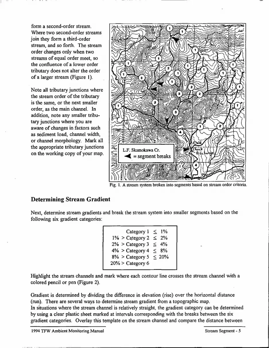
The TFW Ambient Monitoring Program uses a combination of indicators developed by Dunne and Leopold (1978) to delineate the bankfull channels. These indicators are used to identify the boundaries of the actively changing channel boundaries. The indicators include floodplain level, the shape of the bank, and changes in vegetation (Figure 3). Treat each bankfull width placement as unique and weight all the indicators present equally. There are no key indicators applicable to all situations because most stream systems are in a continual cycle of change due to human or natural disturbance regimes. It is important to remember that indicators respond to the energy of peakflow events and reflect their ability to resist or alter that energy.

alder salmonberry shrub

gravel

Figure 3. Common floodplain, bank/channel, and vegetafive indicators of Floodplain indicators- bankfull channel boundaries.

In channels with natural (un-diked) riparian areas and a low, flat floodplain, the boundary of the bankfull channel is located near the top of the low bank between the active channel and the floodplain. The floodplain may be frequently flooded (i.e., a recurrence interval of greater than 1.5 - 2 years), but the boundary we are looking for is where the energy of the water is no longer sufficient to erode or scour away the bank.

In many streams in forested parts of the state, frequently inundated floodplains are often absent, particularly when the channel is confined between steep hillslopes or is incised into an elevated terrace deposit that is not frequently flooded. This indicator is also not appropriate for streams that have been artificially diked or channelized.


Bank/channel indicators- The shape of the bank as well as the changes in channel substrate size can be indicators of bankfull width locations. Observe the banks closely to determine the extent to where active erosion has made a distinctive change in the shape of the bank. Often the bank will slowly curve down from the terrace or floodplain then abruptly cut almost vertically to the bankfull channel. The point where this change takes place can be a useful indicator except in bankcut or slough-off areas. Also, look for changes in substrate size such as where cobble changes to sand and then to soil.

Vegetative indicators- The bankfull channel boundary is often marked by a distinct demarcation line in the vegetation between lower areas that are either bare or have aquatic vegetation, and higher areas vegetated with perennial vegetation such as shrubs, ferns, and trees. In boulder or bedrock confined channels, it may be marked by the line between bare rock and moss. However, moss is a very poor indicator because it often grows on rocks or wood within the bankfull area.

It is important to remember that the general vegetation line changes over time, retreating due to disturbance during large peak flow events, and advancing during periods between larger floods. Identifying the bankfull channel boundary using vegetative indicators requires caution. The vegetation line can be deceptively low when moisture-tolerant species are present. Reed canary-grass, willow and sedges are examples of plants that may actively invade and colonize areas within the bankfull channel. When using vegetative indicators, use only perennial vegetation greater than I meter in height.

Default system- When situations arise where the bankfull width is impossible to pinpoint, use the following default system. First, locate the point at which you feel confident that you are in the bankfull channel. Second, locate the point at which you feel confident that you are above the bankfull channel either on the floodplain or canyon wall. Use the point midway between these two as your bankfull width for that bank.

Other situations- Sometimes it may be possible to identify the height of the bankfull channel on one side of the channel but not the other. For example, this often occurs when there is a low floodplain with vegetative indicators on one side of the stream and a steep, eroding bank on the other. In these cases, extend a level line horizontally across the channel from the side with good indicators to determine bankfull height on the side lacking indicators.

One of the most difficult situations is encountered in stream reaches where large gravel bars have been deposited by large flood events. It can be very difficult to determine if the tops of newly deposited bars protrude above the level of the bankfull channel. Vegetative indicators are unreliable because riparian vegetation is often disturbed during large storm events and revegetation of bars with perennial vegetation may take many years. In these cases, examine the margins of the channel for perennial riparian vegetation and extend a horizontal line across the channel to determine if the bar tops are above or below the bankfull level. If you are still in doubt after doing this, include the area within the bankfull channel.

In other cases, physical obstructions such as debris jams, undercut banks, or a complete lack of indicators may make determination or measurement of bankfull dimensions impossible at the reference point (Figure 4). In these cases, take the measurement at the nearest place where it is feasible and note the distance up- or downstream on Form 2 or in your field notebook.


Aoodjllaln (LeitBanIQ

Criteria for finding BanldUll Width

• PereITIaI vegeiatlon I'NOOdt stml pIantIls a prime IndIcaIcr - alders - ferns -

• Floodplain bemllndicatcr W caused t:(f 1.5 - 2 'P e.oent

I NoIe: If one bani: does not haIIe definable Ilar1I:fU1 v.Id1h IndIcatcrs. nn tape I fiom good bani: and Ie.<eIIt to de1ennIne opp::sIte b;riS' heIglt

Figure 4. Measuring the bankfull width of channels.

Taking Bankfull Width and Depth Measurements

Tenace(Ri!tot Bril r.reIy If eoJer

ftooded

To measure bankfull width, securely attach the end of the fiberglass tape measure at one boundary of the bankfull channel. Extend the tape across the channel to the other boundary of the bankfull channel. This distance is the bankfull width. If a side-channel is present, add the bankfull width of the side-channel to that of the main channel.

While the tape is stretched between these two points, determine the average bankfull depth. Bankfull depth measurements are taken to the nearest 0.01 meter at regular intervals across the stream channel. The number of measurements depends on the width of the channel (Figure 5). Take measurements at 0.5 meter intervals in channels less than 5 meters in width, at 1 meter intervals in channels between 5 and IS meters in width, at 2 meter intervals for channels between 15 and 25 meters, and every 4 meters in channels greater than 25 meters in width. In addition, take an initial measurement 0.1 meter out from the starting point, and 0.1 meter before the endpoint.

Bankfull depth is the distance from the channel bed to the estimated active water surface elevation at bankfull flow, represented by a tape stretched horizontally between the bankfull boundaries. The depth of water at the time of the survey, or its absence, does not affect this measurement. Record all depth measurements in the Field notes section on Form 2 or your field notebook for error checking documentation. The sum of all depth measurements are then divided by the number of measurements taken to compute average bankfull depth. The result is rounded to the nearest 0.1 meter. All calculations need to be error-checked at least once - note when this has been done on Form 2.


Depths !al:en at regular in1efVa1s on the !ape according to banl:llill width

R1ght~ln banl:llilllNldth

width exposed bar

Banl:llill Width of: < m

5m> 15m 15m>25m 25m>

Figure 5. Measuring bankfull depth.

Canopy Closure Measurement

ElevatIon ofwa1Ef Ie.IeI at banldiJl ftc7N used 10 position tape

Note: lal:e additional depth measurements at .1 m fiom each end of the tape and average with all depths

Canopy closure measurements are taken at every reference point This measurement is an average of four systematic canopy closure readings taken in the middle of the wetted channel along the reference point cross-section.

To take a densiometer reading, hold the densiometer 12-18" in front of you at elbow height Use the circular bubble-level to ensure that it is level. Look down on the surface of the densiometer, which has 24 squares etched into its reflective face. The reflection of the top of your head should just touch the outside of the grid. Imagine that each square is SUb-divided into four additional squares, so that there are 96 smaller quarter-squares. Envision a dot in the center of each quarter-square. Count the total number of quarter-square dots covered by the reflection of vegetation (Figure 6). Read the number to your partner who records them on in the appropriate column of Form 2.

To measure canopy closure systematically, four readings are made with a densiometer. Begin with a reading facing directly upstream (Up); then turn clockwise 90 degrees and take a reading facing the left bank (LB); then turn another 90 degrees clockwise and take a reading facing downstream (On); and fmally turn clockwise another 90 degrees and take a reading facing the right bank (RB). For Canopy Closure: sum the number of quarter-square dots obscured with vegetation for all four readings; multiply the result by 1.04 (correction factor); and divide this result by 4. The result is the average percentage of canopy closure at that reference point and it is recorded in the "%" column on Form 2.

If more than one channel is present at the site, take canopy closure measurements in the main channel and each side channel (e.g., main channel = 75%, side channel A = 85%, side channel B = 95%.)

1994 TFW Ambient Monitoring Manual Reference Point - II

Head Reflection Top Line Crosses Top of Head

Bubble Leveled

Figure 5. View into a convex spherical densiometer showing placement of head reflection and bubble level. Visualize four equi-spaced dots in each square and count the number covered by vegetation. Note: Concave densiometers are also available.

Next, measure the wetted width of each channel and then divide the wetted width of each channel by the sum of the wetted width of all the channels to determine the percentage of the total width provided by each channel (main channel = 85%, side channel A = 10%, and side channel B = 5% of the wetted width.) Multiply the canopy closure measurements for each channel by its respective percentage of the total channel width (main channel: 75 X .85 = ill , side channel A: 85 X .10 =.8...5. , and side channel B: 95 X .05 = 4..8..) Finally, sum these measurements to determine the average canopy closure at the reference point (63.8 + 8.5 + 4.8 = 77% adjusted canopy closure.) Record this number on Form 2. All calculations need to be error checked at least once - note when this has been done on Form 2.


Filling Out the Reference Point Survey Form 2

:fwo options are available for recording information collected in the Reference Point Survey. Use the regular Reference Point Survey Form 2 (Appendix A) to record your data if you want to enter it by hand into the database. Use the scannable version Form 2 (Appendix B) to record your data if you want to scan the data directly into the database. The hand-entry version has is laid out and has space included for field notes and writing actual measurements used in calculations. Using this space or keeping detailed notes provides error-checking documentation. The following section describes how to record data on this form.

Background information - Begin a new form at the start of each day and completely fill-out the header information on each sheet used during the survey. Number the sheets sequentially for the entire segment (e.g., I of 10, 2 of 10 and so forth). Record the Water Resource Inventory Area (W.R.I.A.) number segment number, and survey start date. Next, record the Stream Name, Basin Name, and beginning and ending Rivermiles for the segment. Next, record the names of the crew leader and recorder(s) for the survey and note the actual date of the survey.

Reference point number - Record the number of each reference point in this column, beginning with reference point #0 at the lower boundary of the segment. Note if the tag was placed on the left bank, right bank, or both (right and left bank are always determined looking downstream.)

Cumulative distance - Record the cumulative distance (in meters) from the lower boundary to each successive reference point. For instance, when the reference points are laid out at 100 meter intervals, the cumulative distance to reference point #0 would be 0 meters, to reference point #1 would be 100 meters, to reference point #2 would be 200 meters, and so forth. If one or more of the reference points are not laid out at 100 meter intervals, record the actual cumulative distance and adjust the next reference point placement to bring the cumulative distance back to an even hundred meter position (e.g., RP# 3 cum. dist. @ 294 meters; RP# 4 cum. dist. @ 400 meters).

Photographs - Record the roll and frame number for both the upstream and downstream photographs.

Bankfull width - Record the bankfull width measurement at each reference point to the nearest tenth of a meter.

Bankfull depth - Record the avera&<: bankfull depth at each reference point to the nearest 0.1 meter. This number is computed by adding together the individual bankfull depth measurements (recorded in the Field notes column to the nearest 0.01 meter) and dividing them by the number of measurements taken (see measuring bankfull width and depth, above).

Canopy closure - Record each of the four systematic canopy closure readings (sky obscured by vegetation) in the appropriate space on the hand-entry Form 2. Calculate the average percentage of canopy closure (sum the four readings; multiply by 1.04; divide by 4) and record this number in the % column.


Data Processing and Analysis

After data has been hand entered (by the cooperator) or scanned into the database, it is error checked back to the original field form. When all errors have been corrected, reference point survey information is summarized in the Stream Segment Summary Report (Appendix C). This report provides information including: average bankfull width, average bankfull depth, width/depth ratio and average percent canopy closure. In addition, cooperators receive a copy of the database on floppy disk for their use. Data is also stored in a statewide database at NWIFC for future TFW-related use.

Training, Field Assistance, and Quality Control

This manual is intended as a reference for those collecting monitoring information using the TFW Ambient Monitoring Program Reference Point Survey Module. Because of the difficulty in relying solely on a manual to learn and implement monitoring methodologies, the TFW Ambient Monitoring Program offers formal training sessions and informal field assistance visits to help cooperators learn and implement the methodologies.

In addition, the Ambient Monitoring Program also provides a quality control service that involves having an experienced crew perform replicate surveys for cooperators. The purpose of these surveys is to identify and correct inconsistencies in application of the methods and to provide documentation that data is being collected in a replicable and consistent manner throughout the state. The quality assurance service entails both pre- and mid-season QA surveys. The pre-season QA survey documents that your crews are collecting high quality data from day one. The mid-season QA survey documents crew consistency and whether training or corrections applied to problems during the first QA survey were effective. For more information on quality assurance protocols, refer to the Quality Assurance Module.


References

Dunne, T. and L.B. Leopold. 1978. Water in environmental planning. W.H. Freeman and Co. New York.

Richards, K. 1982. Rivers: form and process in alluvial channels. Methuen. New York.

Schumm, S.A. 1977. The fluvial system. Wiley-Interscience. New York.


APPENDIXES

Appendix A Reference Point Survey Fonn 2 - hand entry

AppendixB Reference Point Survey Fonn 2 - scan entry

Appendix C Stream Segment Summary Report sample


*

Field Form TFW Ambient

REFERENCE POINT SURVEY

Stream Name Basin Name Rivermile from to

Crew Lead ____________ _ Recorder

Cumulative

I W.R.LA., , Segment#-- -----OLBC)'RB

Survey Start Date _,_, __ Survey End Date _,_, __ Fill out all infonnation on every fonn. Full

names req~ired on flnt fann for each day· • inifials can be used on secondary pages

Affiliation Survey, Date _'_' , __

Field Notes (R<£pL distance from bank, tree type, list all

BFD~~'::"ts,~

'5 ~1--------r---r---------+---+---+---+--------+--------1_-t~r_+-_r----~--------------------------~

,S ~

~r--------r---+-----------r---+----r---+---------4-------~~~--~~--4-----~~----------------------------~

Jr-------r---r---------+---+---+---+-----~-+------~1--+~r-+--r----~--------------------------~ ~

* 1---------t---+-----------r---+----r---+---------4_---------r~~~~--4_----~~----------------------------~

Northwest Indian Fish.:ries Commission. 6730 Martin Way E., Olympia, WA 98506 (206) 438-1180 g:\rnanual94\form2.pm4

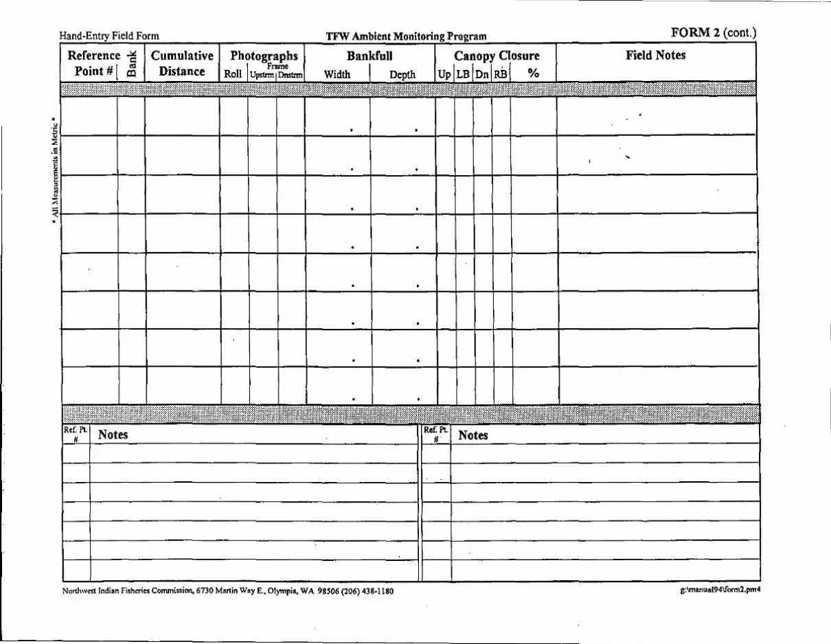
• o

Field Form

Cumulative

TFW Ambient FORM 2

Field Notes

.~

~~----~--+--------+--4---~-4----~-+----~-+-4~~~+---~~----------------------.5

i~------~--~---------4--~~--~--+-----~~~----~-+--+-~-4--+------+--------------------------~ ~ o ::;

•

Northwest Indian Fisheries Commission. 6730 Martin Way E., Olympia, WA 98506 (206) 438·1180 g:l.rnanuaI94\fonnl.pm4

TFW Ambient Monitoring FORM 2

REFERENCE POINT SURVEY

Use a No~ 2 pencil. Fill bubbles darkly and completely. Do not make stray marks. Page_of_.

STREAM NAME

REFERENCE POINTS "n"

o 000~~'JK 000

2 f2\ f2\ 0 RIGHT 'V'V BANK

300 000 ®®® 6®@ 000 @@0 000

"n +, .. "

o 0@O~~K '00 2 f2\ f2\ 0 RIGHT

'V'V BANK 300' 400 5®® 6®0 700 000 '0®

REFERENCE POINTS -n + 2" . "n + 3"

o I(i\ I(i\ 0 LEFT "'-' "'-' BANK

000 0000~~~~ 300 000 5®® @@@ 700 000 .®®

rev, 8/92

®0@O~~'JK 000

2 f2\ f2\ 0 RIGHT 'V'V BANK

300 400 5®® 6®0 000 B00 • • 0

DATE

MO.

I

CUMULATIVE DISTANCE 1m)

0000 0000 0000 0000 0000 ®®®® @0®® 0000 00®0 '000

CUMULATIVE DISTANCE {ml

I I I ,00@0 0000 0000 0000 0000 ®®0® @@0@ 0000 0000 0000

DAY

I YR.

I

CONF.! GRAD.

PHOTOGRAPHS u D

ROLL FRAME FRAME

I I' ! U LL 000 070' 00 00q:

';: 00 00

000 00 "00 000 00 00 ~00 """~ =0 ®®® l@ ® ~00 @ 0 000 0 . 0 000 0 0 0®® ,r.,

~ ,,;.

PHOTOGRAPHS . U,. D

ROLL FRAME FRAME

0@ 00 0 2

30 o ® @ o B

•

00 00 00 0 3

o ® o o o •

W.R.I.A. NUMBER'

CANOPY CLOSURE

000 '00 00 00 00 ®® 00 00 0 B

00

CANOPY CLOSURE

000 '00 00 00 00 ®® @0 00 0 B

Continue on back of form"

UNLISTED SEGMENT

TRIB NUMBER

BEGINNING RIVER MilE

I I !

BANKFULL WIDTH DEPTH

BANKFULL

WIDTH DEPTH

I I . • 000 0 00 @ 000 0 00 0 0000000 00001ill,0!@ 0000 00 ~®®@ ~® 00@0 0@ 0000 ~0 0000 ~0 0000 ~ill

ENDING RIVER MILE

I I !

> ~ ~ t!!'j

~ S< =

8 N • <

;; ~ ~

N

~ m • ~ ~ u z > ~

". • ;; ~

~ ~

• ~

~ ,< ~ • ~

• • •

© NW Indian Fisheries Commission

•

• • • I

utie a 1\10. L. pencil. 1"IIIIJuIJbles aarl<1y ana completely. Uo not mal<e stray marl<s.

REFERENCE POINTS

REFERENCE POINTS

REFERENCE POINTS

"n + S" "n + 9"

@@o o LEFT BANK 000 000 o RIGHT

BANK 000 000 00' 0@@ 00 7

®@® '00

I I I I I I I I

CUMULATIVE DISTANCE (m)

-Ill @@@@ 0000 0000 0000 0000 @000 @@@® 0000 @@®® 00(.)0

CUMULATIVE DISTANCE 1m.

@@@@ 0000 0000 0000 0000 @@00 ®®®® 0000 ®®®®

CUMULATIVE DISTANCE 1m}

I I I @@@@ 0000 0000 0000 0000 0000 0®@@ 0000 @®®® 0(.)®0

I I I I

PHOTOGRAPHS U D

ROLL FRAME FRAME

4

• @ @ •

7

® ,

PHOTOGRAPHS U D

FRAME FRAME

I I I I I I I

CANOPY CLOSURE

CANOPY CLOSURE

CANOPY CLOSURE

@@o 100 00 0' 00 0@ @@ 00 ®. ®®

I II.

BANKFULL

WIDTH DEPTH

. .. @@@@@@)@ '00000 ' 0000000 , 00' , 00 0000 4 4

@00' @@®® 0000 .®®. 0' , ,

BANKFULL

BANKFULL

WIDTH DEPTH

I I ! ! @@@ @ @@ @ 1000 0 00 0 000 0 00 0 000 0 ~0 I@ 000 0 0 0 @@@ @ @ 0 @®@ @ @ @ 000 0 0 0 @@® ® ®@ 0(.)0 ® ~ill

I I I II I I

'-'.'..., - . _.",:

-'

:::>~>. ~<~.:·r

': ~ .~ ~\:.~ ~:';~~ ;~~; ..

, .... : .

.... : .... : .

.... : -•... : ....

'. "

' ... " '. : .

.....

. '.: .. '.;' ';'.::~ . ..... .: ..

:: :

II APPENDIX C II -TFW--Amblent--Monitoring Stream Segment Summary 1992

Stream Segment Identi fication ( FileID: CC ) -----------------------------

StYeam name: WRIA number: Rive\'" mile:

DESCHUTES R. 13.0028 35.3 to

Segment number: '36.6

StYeam Segment Chayacteyistics ------------------------------

18

Confinement: U

WAU name:

Gradient category: 2 Avg bankfull width: 20.2 M Segment length: 2615.0 M

Avg bankfull depth: 0.4 M Uppey elevation: 550 r

•

WAU #:

StYeam order: 4 Width / depth: 46.66 Lower elevation: 510 F

.. ~ •.. ---.-.------.----- '·P"c~"""":U.N=a. ,,_~-...,=~===-- _ .. '- --.... ---- .. - .


HABITAT UNIT SURVEY MODULE

August 1994


Lyman Bullchild



Contents


Introduction .............. .................................................................................................. 3

Purpose of the Habitat Dnit Survey Module ................................................................ 4

The Habitat Dnit Methodology ................................................................................... 4

Infonnation and Equipment Needed .......................................................................................... 4 Discharge ............................................................................................................................... .... 6 Identification of Habitat Units ................................................................................................... 8 Channel Location of Habitat Units ........................................................................................... 13 Measuring Lengths and Widths of Habitat Units ...................................................................... 15 -Splitting Units at Reference Points ........................................................................................... 20 Determining Residual Pool Depth ............................................................................................ 20 IdentifYing Factors Contributing to Pool Fonnation ................................................................. 22

Filling out the Habitat Dnit Survey Form .................................................................. 23

Header Infonnation .................................................................................................................. 24 Habitat Unit Infonnation ......................................................................................................... 25

Data Processing and Analysis.. ......... ............................. ....... .................................... 26

Training, Field Assistance and Quality Control .. ....................................................... 26

References ........................................................................................ _ ...................... 27

Appendixes ........ ....................................................................................................... 29

J 994 TFW Ambient Monitoring Manual Habitat Unit - J

Acknowledgements

Thanks to Bruce Baxter, Carol Bernthal, Phil DeCillis, Larry Dominguez, Paul Faulds, Hugo Flores, Brian Fransen, Jeff Light, Mark Mobbs, Ed Rashin, Mindy Rowse, and Jim Ward for contributing ideas, comments and field assistance during the development of this module.

Cover photograph by Allen Pleus. Lyman Bullchild (L) and Joe Apfel measuring a pool unit on the West Fork Teanaway Creek, 1991.

1994 TFW Ambient Monitoring Manual Habitat Unit - 2


Introduction

Hydraulic conditions such as water depth and velocity vary within stream channels. This variation often occurs in somewhat orderly patterns with distinct, alternating areas of deep water (pools) and shallow water (riffles). These distinct areas are referred toas "habitat units" (Figure 1).

Various species and life history stages of aquatic organisms have adapted to the rigors and opportunities presented by particular hydraulic conditions. Consequently, they are more likely to be found in particular habitat units (Bisson et al., 1982). The type and amount of habitat units present in a stream reach can be used as an indicator of its suitability for a particular species or life history stage.

Intrinsic factors such as stream size, gradient and confinement influence the type and relative abundance of habitat units found in a particular reach (Beechie and Sibley, 1990). In addition, the relative abundance and characteristics of various habitat units responds to changes in 10caI- and watershed-scale processes that determine sediment supply, runoff during storm events and recruitment of large woody debris. These processes and their inputs may be altered by human activities such as forest practices and by changing natural conditions.

Figure 1. Lyman Bullchild (foreground) and Joe Apfel measuring the length ofa rille unit. West Fork Teanaway Creek. 1991.

Because the utilization of instream habitat varies by species, life history stage and physiographic region, no single habitat survey methodology can accurately characterize habitat conditions for all salmonids throughout the State of Washington. Instead, the habitat unit survey focuses on partitioning streams into basic morphological features. The intent of the survey is to characterize current


morphological conditions, and to monitoring changes in the size and frequency of these units in response to changing inputs of sediment, discharge and large woody debris associated with natural or management-induced disturbance and recovery.

Purpose of the Habitat Unit Survey Module

The purpose of the habitat unit module is to:

I. Provide a means of accurately characterizing the current status of basic channel morphology at a level of precision and detail suitable for use as a foundation for monitoring.

2. Provide an accurate methodology that can be repeated over time to document changes and trends in habitat unit frequency and abundance.

3. Provide information on the percentage of pools suitable for use as a resource condition index in the Watershed Analysis cumulative effects assessment procedure.

The Habitat Unit Methodology

This section describes procedures for identifying and measuring the characteristics of habitat units. The habitat unit survey uses a classification system consisting of four "macro" habitat units (pools, tailouts, riffles, and cascades). The change to the four unit system from the more complex microhabitat unit system used prior to 1992 was made to improve observer recognition of units and to improve our ability to replicate surveys. See Ralph et a1. (1991) for a discussion of replication problems with the micro-habitat system.

Please record all measurements in metric units to reduce confusion and streamline data processing. The decision to use metric units was made because most scientific studies used for comparison and interpretation of monitoring data are reported in metric units.


In order to complete the habitat unit survey, it is necessary to have previously identified a stream segment to survey (see the Stream Segment Identification Module). It is also necessary to have established reference points (see the Reference Point Survey Module) so the habitat units can be associated with a permanent reference location. In addition, you will need to know the average bankfull width for the survey segment. To determine the average bankfull width of the segment, examine the completed reference point survey forms for the segment, sum the bankfull width measurements and divide by the number of measurements.


You will need the following equipment to conduct the survey:

* Fiberglass tape (metric) * Stadia rod (metric) * Abney level or clinometer * Electronic or Optical rangefinders Flow meter Wading rod for flow meter Hip boots or waders (* Calibration required)

Calibration

Habitat unit survey forms (Form 3) Clip board or form holder Field notebook Map Number 2 pencils First aid supplies Insect Repellant


All linear measurement equipment is calibrated against a designated 50 meter fiberglass tape (a 30 meter tape will work ifit the longest or best you have). To designate your calibration standard tape, choose the newest equipment that does not have any breaks or splices for its entire length. The accuracy of the calibration standard is determined by comparing it to other tapes that are not spliced or broken. Once you have designated a fiberglass tape, identify it as such by writing "Calibration Standard" in permanent marker on the housing and include the date.

To calibrate other equipment to your standard, find an open area and roll out the tape in a straight line with the zero end anchored. The Habitat Unit Survey Module has several pieces of equipment which need to be calibrated at least once per year as follows:


Stadia Rod: Place the stadia rod parallel to the calibration standard with the zero ends at the same point. Check the accuracy of the markings to the 0.01 meter level for the first 2 meters and the rest at the 0.1 meter level. Check the rod for damaged and illegible markings. Locking buttons are often replaceable if they no longer function properly. Illegible markings can be fixed by permanent marker if not too severe. Avoid using any correction factors for damaged equipment.

Abney Level or Clinometer: To measure water surface gradients for determining cascade and riffle units, it is necessary to use the instrument to mark your eye-level on a stadia rod or measuring stick. First, find an area that is level such as the floor in your office. Parking lots are not good locations because most of them are sloped to aide rain runoff Next, extend the stadia rod out and have your partner hold it I meter away with the zero end on the ground and the rod vertically level.


The person holding the abney level or clinometer should stand in a normal position (one that you can consistently repeat in the field) with their hip or chest waders on and sight the instrument on the stadia rod. Have your partner hold a finger or pencil along the rod and adjust it until they intersect the zero or level mark on your instrument. Use a permanent felt pen to mark your eye-level position on the stadia rod. Repeat this process for all crew who will be making this measurement, if you buy new boots, and if you use different boots.

Electronic and Optical rangefinders (metric): Electronic rangefinders must be calibrated daily and optical rangefinders must be calibrated at least twice daily and more if needed. Use your calibration standard tape and check the accuracy of your instruments at 5, 15, and 30 meter intervals. Adjust instruments according to manufacturer guidelines and stated accuracy ranges. Note: Optical rangefinders are the least precise measurement instrument and it is recommended that cooperators do not use them.

Discharge

The suTface area of the wetted channel and individual habitat units changes with discharge, so measurements are affected by the amount of water flowing in the channel at the time of the survey. The Habitat Unit Survey methodology is designed to be applied during relatively stable flow conditions characteristic of the summer low flow period. Surveys should not be conducted during periods of high water associated with summer storms, during extreme low base-flow conditions when sections of typically perennial streams are dry, or during periods of rapidly fluctuating discharge.

Discharge should be measured at the time you begin to survey each segment and every subsequent week until the survey is completed. If discharge changes significantly during the time the segment is being surveyed, additional discharge measurements need to be taken. As a general rule, take a discharge measurement any time the flow changes by +/- 10%.

In order to obtain comparable data, future surveys of the same segment should be conducted at a discharge similar to that of the original survey. At this time, the sensitivity of the methodology to changes in discharge has not been determined. Pending further analysis, we recommend that discharge at the time of repeat surveys be +/- 10% of the discharge during the original survey.

Discharge should be determined using the following standard stream flow measurement methods. Begin by selecting a suitable location (within the segment being surveyed) with adequate depth and smooth, laminar flow. A suitable site should not have flow diversions, side-channels, or undercut banks. Select sites relatively free of turbulence and flow obstructions such as large rocks, logs, and aquatic vegetation.

Stretch a fiberglass tape across the wetted portion of the stream channel perpendicular to the direction of flow. Attach each side of the tape securely and note the distance on the tape corresponding to the water's edge on each side of the stream. Next, assemble your flow meter and test it to ensure that it is working properly. A variety of flow meter designs are available that are suitable for this purpose. Operate your meter according to instructions provided by the manufacturer.

The next step is to divide the stream cross-section into cells and to measure water depth and velocity

1994 TFW Ambient Morutoring Manual Habitat Unit - 6

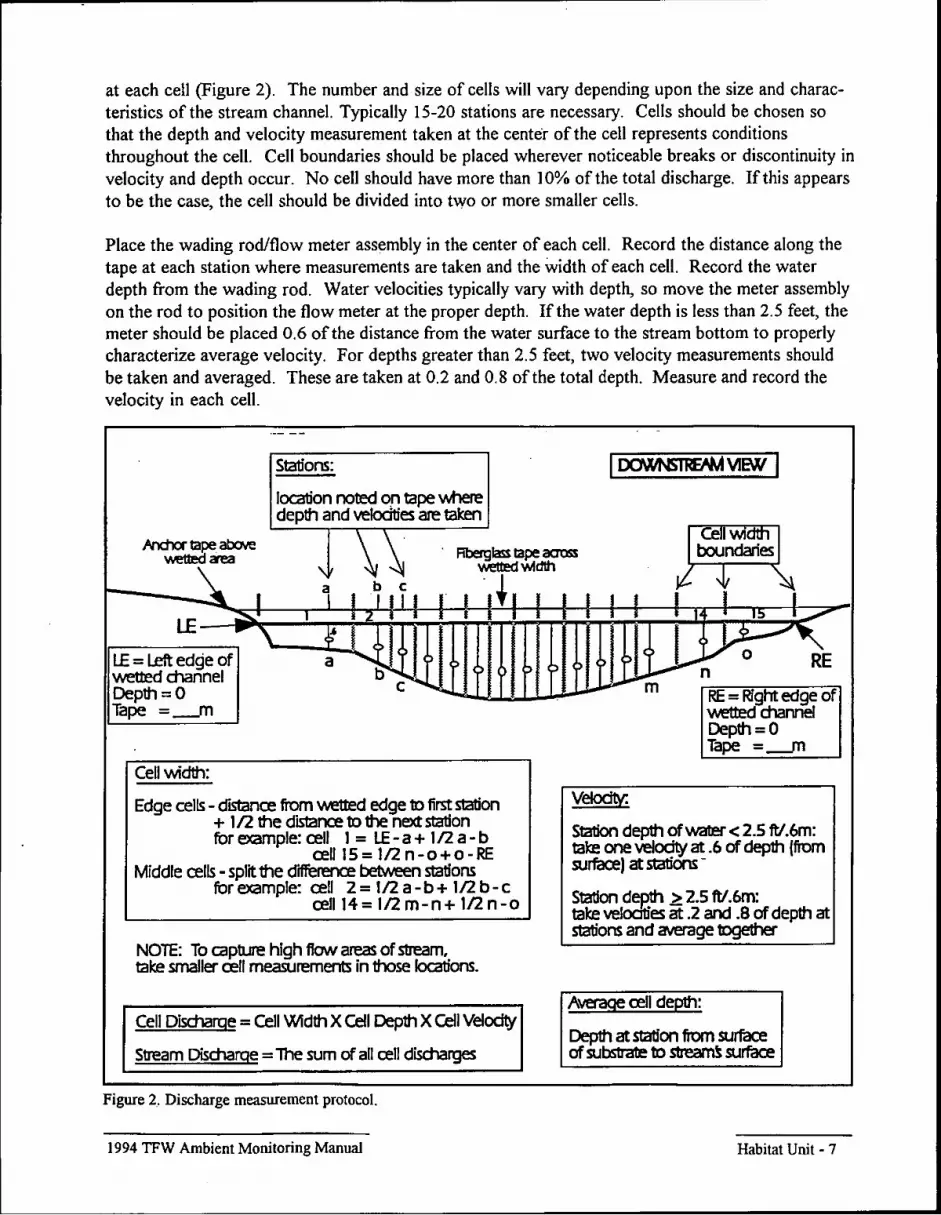
at each cell (Figure 2). The number and size of cells will vary depending upon the size and characteristics of the stream channel. Typically 15-20 stations are necessary. Cells should be chosen so that the depth and velocity measurement taken at the center of the cell represents conditions throughout the cell. Cell boundaries should be placed wherever noticeable breaks or discontinuity in velocity and depth occur. No cell should have more than 10% of the total discharge. If this appears to be the case, the cell should be divided into two or more smaller cells.

Place the wading rod/flow meter assembly in the center of each cell. Record the distance along the tape at each station where measurements are taken and the width of each cell. Record the water depth from the wading rod. Water velocities typically vary with depth, so move the meter assembly on the rod to position the flow meter at the proper depth. If the water depth is less than 2.5 feet, the meter should be placed 0.6 of the distance from the water surface to the stream bottom to properly characterize average velocity. For depths greater than 2.5 feet, two velocity measurements should be taken and averaged. These are taken at 0.2 and 0.8 of the total depth. Measure and record the velocity in each cell.

.- -

Stations: I~VlBVI

location noted on tape where depth and velodties are taken

Hldlor tape aboIie \\ ~ Rberglass tape across boundaries

~~ , WetII!d wldIh

I , . ~ I I I • f i 1

LE I I I ......

\. .J;' I ;, ./

( ,...../0 LE = Left edge of a ...... '0 RE wetted channel ........... n Depth =0 c m RE _ Right edge of Tape =-"1 wetted channel

Depth = 0 Tape =-"1

Cell width:

Edge cells - cflStance rom wetted edge 10 first station VeIodtv: + 112 the distance 10 the next station Station depth of water < 2.5 ftI.6m: for example: cell 1 = LE-a+ 112 a-b

cell 15= Il2n-o+o-RE take one velocity at.6 of depth (fi"om

Middle cells - split the difference between stations surface) at stations -for example: cell 2 = 112 a - b + 112 b - c Station d~ ~ 2.5 ftI.6m: cell 14 = 112 m-n + 112 n-o take velOCities at .2 and .8 of depth at

stations and average together NOTE: To capture high flow areas of stream. take smaller cell measurements in those locations.

Average cell depth: Cell Discharge = Cell Width X Cell Depth X Cell Velocity

Depth at station fi"om surface Stream Discharge = The sum of all cell discharges of substrate 10 stream~ surface

Figure 2. Discharge measurement protocol.


To determine the total discharge: (I) calculate the discharge for each cell by the multiplying cell width by the water depth to produce the cross-sectional area; (2) multiply the cross-sectional area by the velocity to get the discharge; and (3) sum the discharge measurements for all cells to calculate the total discharge. An example of a completed discharge measurement Form 7 is shown in Appendix A. A blank discharge measurement Form 7 that can be copied for field use is included in Appendix B. The form also contains a formula for converting cubic feet per second (cfs) to cubic meters per second (cms).

Identification of Habitat Units

The first step in this procedure is to determine the type of habitat units present. Wetted portions of the main channel and side channels where water is present are assigned to one of four habitat unit

Pool Riffle

Habitat Units

Cascade Tailout Obscured Wetland Sub-Surface Flow

=

=

= =

= = =

P R C T o W 8

Figure 3. List of Habitat Units and single letter codes.

types, pool (P), riffle (R), cascade (C), or tail out (T). When portions of the channel are not visible, for example when it passes under a massive debris jam or through a long culvert, it is designated obscured (0). If it dissipates into a wetland without a distinct channel, it should be designated as a wetland (W). If the main channel is dry it should be designated as sub-surface flow (8) (Figure 3).

To qualifY as a pool, riffle, cascade, or tailout a potential unit must meet a minimum size criteria. The minimum size requirement for a habitat unit varies with channel size, expressed as bankfull width (Table 1). Areas that do not meet the minimum size criteria should be combined with the

most similar adjacent unit.

Table 1. Minimum unit size by channel bankfull width.

Channel Bankfull width (meters)

0 2.5

2.5 5

5 10

10 15

15 20

> 20

Minimum unit size (square meters)

0.5

1.0

2.0

3.0

4.0

5.0

Characteristics of Habitat Units

The purpose of the minimum unit size criteria is to provide guidance and improve consistency between observers who tend to lump and those who tend to split units. A consistent minimum size criteria is also necessary to reduce variability associated with crew bias towards identifYing smaller units of a particular habitat type. This can often be a problem where a cooperator is only interested in· pooVriffie ratios and does

not quantifY "small" cascade units.

Once the minimum size criteria is met, pools, riffles, cascades, and tail outs are distinguished on the basis of several hydraulic and geomorphic factors such as depth and gradient.

Pools- Pools are areas of deep water with low water surface gradients (generally less than I %). They are typically created by scour adjacent to obstructions or impoundment of water behind

1994 TFW Ambient MonitOring Manual Habitat Unit - 8

channel blockages and hydraulic controls such as logjams, bedforms or beaver dams. To qualify as a pool, a unit must not only the minimum surface area size criteria, but also meet a minimum residual depth requirement based on the same bankfull width scale.

Riffies- Riffles are shallow, low gradient areas that do not meet the residual pool depth requirement. They are distinguished from cascades by having a water surface gradient ofless than 3.5 percent. Many riffles exhibit surface turbulence associated with increased velocity and shallow water depth over gravel or cobble beds. However, the riffle classification also includes shallow areas without surface turbulence such as glides and pocketwater conditions that do not meet the minimum pool depth requirement.

Cascades- Cascades are steep areas with a wat.er surface gradient exceeding 3.5 percent. Some cascades are very short and smooth, such as slip-face cascades located on the downstream faces of channel bars or bedrock outcrops. Step-pool cascades occur where boulder or cobble substrate forms stair-steps. They often are very turbulent, and have numerous small pools associated with the cobblelboulder steps.

Tailouts- Tailouts are situated on the downstream end of pools, in the transitional area between the pool and the head of the downstream riffle. They are areas of moderately shallow water with an even, laminar flow and a lack of pronounced surface turbulence. These units provide deposition sites for fine bedload materials (Lisle 1982). They have a flat, smooth bottom, lacking the scour typically associated with the pool. Because they are located on the upstream side of the riffle crest, they lack the velocity and surface turbulence associated with riffles or cascades located on the downstream slope of the riffle crest. Tailouts are most commonly found in larger, low-gradient channels associated with elongated pools that have well-sorted substrate. They are uncommon in small, highgradient streams with coarse substrate.

Using Minimum Residual Pool Depth to Distinguish Pools

Although some pools are quite distinct, in many cases it is difficult to differentiate shallow pools from deep glides or riffles. Considerable divergence occurs in habitat calls made by experienced observers in these situations. To eliminate this problem and provide consistent, replicable survey results, a criteria for minimum residual pool depth has been established. A pool must exceed a minimum residual pool depth criteria that corresponds with channel size, expressed as bankfull width (Table 2).

To determine if a potential unit qualifies as a pool, take a residual depth measurement (see the "Determining Residual Pool Depth section below), and compare with the minimum value for the appropriate channel size using the average bankfull width computed from your Reference Point Survey Form 2.

1994 TFW Ambient MonitOring Manual

Table 2. Minimum residual depth criteria for pools by channel bankfull width.

Channel Bankfull Minimum Residual width (meters) Pool depth (meters)

0 - 2.5 0.10

2.5 - 5 0.20

5 - 10 0.25

10 - 15 0.30

15 - 20 0.35

> 20 0.40

Habitat Unit - 9

If the minimum residual depth requirement is met, the next step is to establish the boundaries of the pool unit and determine if it meets the minimum unit size requirement. In most cases, pool boundaries extend laterally to the waters edge. However, if there is a riffle or cascade unit adjacent to the pool that meets the minimum unit size criteria, it should be treated as a separate, adjacent unit.

Delineating the upstream, downstream, and adjacent boundaries of pools to other units can be difficult. The variety of situations encountered make the use of a single boundary indicator impractical. Look for distinct changes in water surface gradient, surface turbulence, water velocity, direction of flow, substrate size, and channel morphology. It is important to weight all indicators together when making unit boundary decisions. Factors which make identification of boundaries difficult are water clarity, reflection of the sun, heavily shaded areas, and areas obscured by vegetation or overhanging banks. The use of weighted flags (Figure 4) is helpful in marking and remembering boundary locations for accurate surface area measurements.

In situations where the boundary between the pool and another unit is indistinct, use the following default method. First, use weighted flags to mark the boundary point where you can distinguish a definite pool unit. Next, mark the boundary point where you can definitely distinguish the other unit's boundary. Place a third flag half-way between those marks and remove the other two. This is your pool boundary.

Distinguishing Tailouts

flagging material

12" -----.l~1

1 oz. lead "bank" sinker

Figure 4. Weighted flag for helping mark unit boundary and other instream locations.

Once a pool has been identified, the next step is to determine if a tail out unit is present at its lower end. Often, a gradual increase in velocity and decrease in depth occurs in a transitional tail out area below larger, elongated pools. In these situations, the boundary between the pool and the tailout is delineated by examining the bedform of the channel and determining the downstream extent of distinct streambed scour. Where the cross-sectional profile of the bed becomes even and flat, the downstream boundary of the pool has been reached. The area below this boundary IS designated as a tailout (Figure 5).

The tail out extends downstream to the riffle crest, where the water increases in velocity as it flows down the downstream slope of the crest. This boundary is typically distinguished by surface turbulence associated with the riffle or cascade. Most pools, particularly smaller pools in moderate to high gradient channels, do not have distinct tailouts because the zone of scour extends to the riffle crest. In these cases, extend the pool unit to the riffle crest and do not delineate a tailout unit.

In situations where the boundary between the pool and the tailout is indistinct, use the following default method. First, use weighted flags to mark the furthest downstream point where you can distinguish a definite pool unit. Next, mark the furthest upstream point where you can distinguish a

1994 TFW Ambient Monitoring Manual Habitat Unit - IO

-'" 'e

c:: e. ~ , --

--- -------------------------------------,

Fig.la

Fig. Ib

Fig. Ie

Pool outIetlRiffle crest

Riffle

0iteIfa fix calling Tailouts: Same as other habitat units -must meet minimum surface area fix bankfull width.

-- Flow

Tailout

~Flow

Tailout units are designed to help monitor sediment filli~ of pools and provide addittonal habitat resolution

··In riffle and tailout units the substrate forms a relatively unifonn depth aaoss the wetted width.

Pool

I Profile I

"" sediment Increases -13Iout unit leng1h Increases and pooIleng1h decreases

I Crossection I

··The pool unit substrate has a rupped or bowed wetted depth fbrmed I:!Y rurrent or high flow scouring action.

Figure 5. Criteria for Pools and Tailouts.

definite tailout unit. Place a third flag half-way between those marks and remove the other two. This is your poolltailout boundary.

Distinguishing Riflles from Cascades

For the purposes of this survey, areas that do not meet the criteria for pools or tailouts are classified as either riflles or cascades. Riflle and cascade units are distinguished from each other on the basis of water surface gradient. Riflle units have water surface gradients less than 3.5 percent; cascade units have gradients equal to or greater than 3.5 percent.

To measure the water surface gradient of a riflle or cascade, observers are positioned at the upstream and downstream boundaries of the potential unit and parallel to the flow of water across the unit's length. One person stands at the suspected downstream unit boundary water's edge, with the bottom of their boots at the water surface level, and sights through a hand-held Abney level or clinometer at a stadia rod held at the suspected upstream unit boundary with its base held at the water surface by the other crew. The Abney level or clinometer is sighted at a point on the stadia rod equal to the observer's eye-level (see calibration section) and the gradient is read from the instrument. To identify the boundary between a riflle and cascade, look for a gradient break where one side has a water surface gradient less than 3.5 percent and the other side is 3.5 percent or greater.

A common problem among crews is lumping smaller cascade units which meet minimum surface area criteria into a larger riflle unit. The solution is to spend a little more time and take more gradient measurements at smaller distances to determine whether a cascade meets the minimum gradient and surface area size criteria. Remember, if you can measure it and it meets the criteria, you must split it out as a separate unit. The minimum unit size requirement occasionally forces the observer to split more small areas then they are use to. However, using this criteria will improve the repeatability of surveys performed by different observers over time and provide consistent data for comparisons between surveys.

Figure 6. Example of small pool unit within a cascade on Willaby Creek.

1994 1FW Ambient Monitoring Manual

Distinguishing Small Pools and Riflles within Cascades

Cascades with boulder/cobble stair-steps (step-pool cascades) often contain numerous small pools and occasional riflles, posing the question of whether to split them out as separate units (Figure 6). These small pools and riflles should be examined and classified as separate riflle units if they meet the appropriate minimum unit size and water surface gradient requirements (see Table 1); and classified as separate pool units if they meet the minimum unit size and residual pool depth requirements (see Table 2). Small pool units that occur within riflles should be treated in the same manner.

Habitat Unit - 12

Optional Habitat Sub-unit Types

The TFW Ambient Monitoring Program does not train or provide quality assurance for this category. To provide flexibility to those cooperators who wish to collect more detailed information on habitat unit types, the TFW Ambient Monitoring Program provides an optional "Sub-unit Type" category for database entry purposes. The choice of sub-classification system is solely the cooperator's responsibility. However, any sub-unit type system used IIll.lS1 fit hierarchically and consistently into the TFW Ambient Monitoring pool, riffle, cascade, and tailout classification system. Do not use sub-unit types interchangeably such as when using "glides" for a description of both TFW riffles and tail outs.

Sub-Surface Flow Obscured and Wetland Units

In situations where a habitat cannot be classified as either a pool, riffle, cascade, or tail out unit, use the following habitat classifications.

SubcSurface Flow (S) - Occasionally, stream reaches will alternate between wet and dry areas, or be completely dry. If the stream is dry because of extreme low flow associated with drought, it is not an appropriate time to conduct a habitat unit survey because the information generated will not be useful for comparative purposes. On the other hand, if intermittent flow is a typical low flow condition, or if it appears to be resulting from changing conditions such as coarse sediment aggradation, then documenting its occurrence is useful.

When intermittent dry areas are encountered in the main channel, they are recorded as sub-surface flow units. Only main channel sub-surface flow areas are counted and recorded dry side-channels and dry secondary units are !1Qt recorded.

Obscured Units (0)- Sometimes it is impossible to identify habitat units such as when a stream runs through a culvert, under a logjam, or through a large undercut bank. When habitat units cannot be seen or their boundaries cannot be identified, record the habitat unit as obscured.

Wetland Units (W) - Sometimes a stream flows through a wetland area and the main channel becomes indistinguishable from the surrounding vegetation, side channels, and pools. In these situations, classify habitat units upstream or downstream to the first side channel which does not reconnect with the main channel upstream (they become indistinguishable from the surrounding wetland); or ifthere are no side channels, stop when the main channel itself becomes indistinguishable from the surrounding conditions. The area in between is recorded as a wetland unit.

Channel Location of Habitat Units

Habitat units are classified in one of three categories, depending on their location and relative significance within the stream channel (Figure 7). Information on habitat unit location allows determination of the relative abundance of side-channels and main channel habitat during summer low flow conditions. The three categories are:


Crf1Eria for an Island:

II Must have perennial vegetation growing on ~ (e.g., plants which survive cwerwin1er such as alders, wll1ows, COtIOnWOOd, rems, =1

21 Must have a 1eng1h equal 10 at least two ba11:fU1 widths (e.g., for a segmentwfth an average banI:1iJ1I ~ 13m. an Island must be 26m!n length orgreater.1

CatagOIy I - Pril1'lalYunit width covers greater1han 50%~wetted channel width.

CatagOIy 2 -"'l)acent unit width covers less 1han 50% ~wetted channe1 width May be separa1Ied fiom pril1'lalY unit ~ a gravel bar.

CatagOIy 3 -Side<t1anne1 unit channels w1ich ae separated fiom pril1'lalY d1ameI . ~a island.

Figure 7. Habitat unit categories.

Note: Gravel bars of any length wfth or without amuaI vegetation ore not oonsIder Islands for ambient monitor1ng purposes.

Category 1- Primary units. These are the dominant units in the main channel. They occupy at least 50% of the wetted channel width. At any given point along the length of the channel, there can be only one primary channel unit.

Category 2- Secondary units. These are sub-dominant units in the main channel that occupy less than 50% of the wetted channel width. They may be either physically adjacent to a primary unit, lie embedded within a primary unit, or are separated from the primary unit by a gravel bar or obstruction.

Category 3- Side-channel units. These are found in stream channels that are isolated from the main channel by an island. An island must: a) have a length equal to at least two bankfull widths, and b) be colonized by perennial vegetation greater than 1 meter in height. Units separated only by bare gravel bars (regardless oflength) are treated as adjacent units.


Measuring Lengths and Widths of Habitat Units

The lengths and widths of habitat units are measured in order to compute the surface area of each habitat unit. All measurements should be taken to the nearest 0.1 meter reading. During data analysis, the total surface area and relative percentage of each habitat type is calculated.

Measuring Lengths of Pool Riffie Cascade and Tailout Units

There are two length measurement protocols recommended depending upon the complexity of the unit shape. The length protocols are part of the overall design to provide the highest accuracy and consistency of habitat unit surface area measurements possible. The accuracy of unit surface area in regards to length measurements is a factor of: (I) the identification of and access to unit length boundaries; (2) the placement of the length measurement as a true geometric baseline for taking an average width; and (3) the accuracy and precision of the measurement instruments used.

Identification and Access - Consistent identification of the unit type as well as its boundaries is a key factor in surface area accuracy. For length measurements, downstream and upstream boundaries are particularly important. Refer to the previous section on distinguishing habitat units for guidelines on identification. Another accuracy factor is access to the unit boundaries and obstructions within a unit that physically prevent proper length measurements. In these situations, crews must do the best they can in regards to limitations of equipment and safety. Sometimes using multiple measurement equipment such as a fiberglass tape up to the obstruction and a stadia rod that can reach to the boundary is a helpful technique.

Length Placement - The first protocol (General) is geared towards length measurements taken on habitat units typically encountered in Washington stream systems. The second protocol (Complex) is geared for situations where habitat units are more complex due to shape or waterflow.

General: The first protocol is for the types of units generally found during habitat surveys where the stream enters and exits the unit in a linear progression. The use of single, cumulative, or average length measurements is dictated by the shape of the unit.

Single length measurements are best used on units with a straight flow pattern such as in Figure 8. In these situations, habitat unit lengths should be measured from the middle of the boundary with the adjacent downstream unit to the middle of the boundary with the adjacent upstream unit. Using the middle of the unit boundary provides the mean length point of the unit in the stream channel and geometrically balances-out surface areas (Figure 9).

Cumulative length measurements are best used on units which are sinuous such as in

1994 TFW Ambient MonitOring Manual

flow

Figure 8. Using single length measurements on units with straight flow patterns.

Habitat Unit - 15

Areas Compensate

iE--- 1/2 ----)j

Upper Unit

Boundary

Figure 9. Using the mid-point of the unit boundary .

flow

Figure 10. Using cumulative length measurements on units with long or sinuous shapes.

flow

Figure II. Using average length measurements on units whose width is greater than its length.

flow

1994 lFW Ambient Monitoring Manual

Figure 10. In these situations, habitat unit lengths should also be measured from the middle of the boundary with the adjacent downstream unit to the middle of the boundary with the adjacent upstream unit. Measurements should follow the shape of the unit along the center of its width. For instance, if the unit curves around a bend, the measurement should follow the curve, rather than taking the shortest distance between the middle of the upper and lower boundary.

Average length measurements are best used on units whose width is greater than its length as in Figure 11. In these situations, it is necessary to reverse the length/width protocols and first take a single width measurement to provide the baseline for the length measurements. The number of length measurements is relative to the unit's total width and shape. The placement of the length measurements are at a 90· angle to the width baseline (see the "Measuring Average Widths" section below for guidelines on frequency of length measurements).

Complex: The second protocol is for complex units with highly irregular shapes and when a stream enters and exits the unit from the sides. In these situations, habitat unit lengths should use a single measurement connecting the furthest points of the unit (Figure 12).

Length Measurement Instmments - For a twoperson crew on a typical size "Stream, a 30 to 50 meter fiberglass tape is the most accurate and consistent instrument for taking length measurements. The fiberglass tape is preferred for the following reasons: (1) it has the highest accuracy; (2) it does not lose calibration; and (3) the tape provides a visual reference for remembering the length baseline.

Figure 12. Using single length measurements on complex units connecting the furthest points.

-----Habitat Unit - 16

Stadia rods are useful for measuring smaller unit lengths. Electronic rangefinders are lightweight and accurate in many situations, but are marginal in heavily vegetated, noisy or humid conditions. The use of optical rangefinders is discouraged due to low accuracy and precision due to their tendency to lose calibration quickly.

Measuring Lengths of Sub-surface Flow Obscured and Wetland Units

Only length measurements are required for sub-surface flow, obscured, and wetland units. Use the following guidelines to make these measurements.

In areas where the main channel goes dry, the length of the sub-surface flow unit is the distance between the middle of the upper boundary on the last downstream wetted unit and the middle of the lower boundary of the next upstream wetted unit. Use a single point-to-point measurement unless the area is very long and the general curvature of the channel can be determined (Figure 13).

In areas where the wetted portion of the channel is not visible and habitat unit identity or dimensions are not possible to quantifY, the length of the obscured unit is the distance from the middle of the upper boundary on the last downstream unit to the middle of the lower boundary of the next upstream unit. Use a single point-to-point measurement unless the area is very long and the general curvature of the channel can be determined (Figure 14).

In areas where the stream flows into and out of a wetland, the length of the wetland unit is the distance from the middle of the upstream boundary of the last definable unit to the middle of the downstream boundary of the next definable unit. Use a single point-to-point measurement to describe the unit length (Figure 15).

SubSmface Flow

Figure 13. Taking Sub-Surface Flow unit lengths.

Obscured

Figurc 14. Taking Obscured unit lengths.

Measuring Average Widths of Pool Riffie Cascade and Tailout Units

Wetland

Figure 15. Taking Wetland unit lcngths.

Average widths are the second important variable used to determine the surface area of habitat units. The accuracy of the average unit width is a factor of: (1) the identification of and access to unit width boundaries; (2) the placement and frequency of width measurements taken along the length baseline; and (3) the accuracy and precision of the measurement instruments used. Average widths are not measured for sub-surface flow, obscured or wetland units.


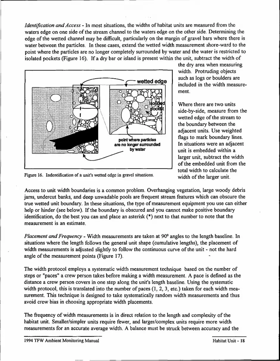
Identification and Access - In most situations, the widths of habitat units are measured from the waters edge on one side of the stream channel to the waters edge on the other side. Determining the edge of the wetted channel may be difficult, particularly on the margin of gravel bars where there is water between the particles. In these cases, extend the wetted width measurement shore-ward to the point where the particles are no longer completely surrounded by water and the water is restricted to isolated pockets (Figure 16). If a dry bar or island is present within the unit, subtract the width of

DOfr,! wt'91B partfclas 8111 no longer surrounded

by water

Figure 16. Indentification of a unit's wetted edge in gravel situations.

the dry area when measuring width. Protruding objects such as logs or boulders are included in the width measurement.

Where there are two units side-by-side, measure from the wetted edge of the stream to the boundary between the adjacent units. Use weighted flags to mark boundary lines. In situations were an adjacent unit is embedded within a larger unit, subtract the width of the embedded unit from the total width to calculate the width of the larger unit.

Access to unit width boundaries is a common problem. Overhanging vegetation, large woody debris jams, undercut banks, and deep unwadable pools are frequent stream features which can obscure the true wetted unit boundary. In these situations, the type of measurement equipment you use can either help or hinder (see below). If the boundary is obscured and you cannot make positive boundary identification, do the best you can and place an asterisk (*) next to that number to note that the measurement is an estimate.

Placement and Frequency - Width measurements are taken at 90° angles to the length baseline. In situations where the length follows the general unit shape (cumulative lengths), the placement of width measurements is adjusted slightly to follow the continuous curve of the unit - not the hard angle of the measurement points (Figure 17).

The width protocol employs a systematic width measurement technique based on the number of steps or "paces" a crew person takes before making a width measurement. A pace is defined as the distance a crew person covers in one step along the unit's length baseline. Using the systematic width protocol, this is translated into the number of paces (1,2,3, etc.) taken for each width measurement. This technique is designed to take systematically random width measurements and thus avoid crew bias in choosing appropriate width placements.

The frequency of width measurements is in direct relation to the length and complexity of the habitat unit. Smaller/simpler units require fewer, and larger/complex units require more width measurements for an accurate average width. A balance must be struck between accuracy and the


of unit

9

to length baseline

to length baseline

Figure 17. Placement of width measurements at 90' angles to the length baseline in relation to unit shape.

time required to make the measurements. As a general guideline, use Table 3 to determine how many individual widths to take in relation to unit length.

For example, if a habitat unit is 15 meters long, you will need to take between 4 and 10 individual width measurements. The pace frequency can be determined by using the following format. If your average pace is about 1 meter long, taking a width at every one pace would produce 13 width measurements; every two paces would produce 7 measurements; and every three paces would produce 4 measurements. Therefore, taking a width every two paces would provide an adequate number of individual widths. As each crew's pace length is different, some experience is required to determine individual pace frequency.

Table 3. Width frequency based on unit lengths

Unit Length # Widths

< 2.5 m 1 - 3 2.5 - S.Om 2 - 4 5.0 - 10.0 m 3 - 6

10.0 - 20.0_m 4 - 10 20.0 > m 8+

NOTE: ~ take width measurements at the downstream and upstream unit boundaries. The general rule is that a width measurement cannot be closer than 1 pace from the beginning or ending unit boundary as defined by the length baseline. Also, be careful when the downstream and upstream boundaries are diagonal across the stream. Adjust your pace frequency to avoid taking widths in these areas as it will result in the calculation of a smaller surface area (Figure 18).


adjust paces to avoid

taking widths in these

areas

Figure 18. Avoid taking width measurements in the areas where the unit boundary ends form diagonals.

Width Measurement Instruments - For a two-person crew on a typical size stream, a 5 meter stadia rod is the most accurate and consistent instrument for width measurements. The stadia rod is preferred for the following reasons: (I) it requires only one person to operate; (2) it does not lose calibration; (3) it's rigidity is useful in probing and reaching wetted boundaries across deep or undercut areas; and (4) it provides an excellent base to gauge 900 angles to the length baseline.

Other equipment such as fiberglass tapes and electronic or optical rangefinder are best used on larger streams and using three-person crews with one person on each bank and the third person providing the pace frequency and 900 angle placement guidelines. The use of optical rangefinders is discouraged due to low accuracy and their tendency to lose calibration quickly. Remember to use weighted flags to mark wetted unit boundaries for accurate surface area measurements, especially for adjacent unit situations.

Splitting Units at Reference Points

To separate habitat unit data into discrete 100 meter reaches it is necessary to be able to divide individual units at reference points. This provides an opportunity to randomly or systematically subsample 100 meter reaches for future monitoring, instead of re-surveying entire segments. It will also provide the opportunity to document and display variation in conditions throughout the segment in 100 meter increments. All types and categories of habitat units are split at reference points. Remember to use weighted flags to mark this boundary for accurate surface area measurements.

To separate the habitat unit data into 100 meter reaches, identifY the units that cross reference points and split them where the reference point intersects the unit. The unit number and type will remain the same, but you will record separate lengths and average widths for each portion of the unit above and below the reference point boundary (Figure 19). Split units require a separate entry on the form for each portion of the habitat unit. Both entries will share the same habitat unit number, but will have different downstream reference point numbers, indicating that they are in different 100 meter reaches. Ifthe unit is a pool, only one entry for maximum depth, outlet depth, and pool forming obstruction should be recorded for the entire unit.

Determining Residual Pool Depth

Residual pool depth is a discharge-independent measure of the depth of a pool relative to the depth of the adjacent downstream hydraulic control structure that controls the total water depth in the pool, such as a gravel bar or a log. It is only measured in pool habitat units. Residual pool depth is used as a criteria for identifYing pools and as a means of monitoring the filling of pools with sediment over time.


Begin sulVe}'where perpendiaJlar line from Ref. PI. 0 crosses d1anneI

Figure 19. Splitting habitat units at reference points.

Assigl these uri! portions to Ref. PI. 0

Ref. PI. 1

Assign these un~ por1Ions to Ref. PI. 1

Where pril11illy. secondaJy. or sidechannel units cross a ,efeie ICe point. spr~ the unit at the line. Make a separate ermy for each poItion eX a unit Both ento1es share the same unit number but have cflfli:rent downs1ream ,ei'ele ICe point rn.mbers. Record the appropriate length and aveoage \Meith measurement for each poItion.

Residual pool depth represents the difference between the elevation of the deepest point (maximum depth) in the pool and the elevation of the lowest point of the crest (outlet depth) that forms the pool's hydraulic control (Figure 20). Residual depth is calculated by subtracting the outlet depth from the maximum depth. To visualize the concept of residual pool depth, imagine what would happen if the water level dropped until it was no longer flowing over the downstream riffle, isolating the pool. The depth of the water that would remain in the pool at its deepest point would be the residual pool depth. See Lisle (1987) for a detailed discussion of residual pool depth.

Maximum Depth - To determine the pool's maximum depth, use your stadia rod to locate the deepest spot in the pool and measure the distance from the deepest point to the surface of the water. You may need to probe around a little to find the deepest spot. In situations where the maximum depth is not accessible (unwadable pools) take the deepest measurement possible and place an asterisk (*) next to the number to note that it is an estimate.

Outlet Depth - To determine the pool's outlet depth, locate the downstream riffle crest or hydraulic control structure that controls the release of water from the pool. The correct location to make the measurement is where the thalweg (deepest part) of the channel crosses the top of the control. It can be visualized as the summit of a mountain pass where the last water will flow past before the pool becomes isolated. You may need to probe around with your stadia rod a little to find the deepest spot. CAUTION: the outlet depth is sometimes located on the side of pool units or in small scour channels along the stream bank.

For dam pools caused by logs or beavers, the deepest point in the water flowing over the obstruction

1994 TFW Ambient MonitOring Manual Habitat Unit - 21

I Note: Resldual Pool depth = Maximum depth - Pool Outlet depth I Pool outlet

depth

Maximum pool depth

Streambed/substrate surface

Figure 10, Measuring maximum pool depth and depth of pool outlet.

I Measure depths rom substrate I surface to water surface

RIffle:

would be the pool outlet depth. If the water is not flowing over the downstream hydraulic control, then the pool outlet depth would be zero. For large cobble or boulder pool outlets (step-pool cascades), the water surface may actually start lowering before it reaches the outlet point. In these situations, do not try to compensate. Follow the standard procedure listed above and measure the depth to the water surface at that point.

Identifying Factors Contributing to Pool Formation

Pools typically form as a result of scour adjacent to channel obstructions or due to impoundment of water behind blockages. Information on the factors contributing to pool formation is collected in order to document changes over time and to provide interpretive information related to current conditions such as percentage of pools and residual pool depth as used in Watershed Analysis.

Table 4 lists a number off actors that often contribute to pool formation. Record any that appear to be contributing to the scour and/or damming effect forming the pool you are observing. Imagine the pool-forming processes at bankfull flow in order to make this determination. Selecnhe primary factor and up to three more, if applicable.

Log, Rootwad or Debris Jam: use the TFW Ambient Monitoring Large Woody Debris Survey Module to identify.

Roots of standing tree(s) or stump(s): applies to pools formed by hydraulic scour when the stream's flow is deflected by the roots of live or dead standing trees and stumps.

Rock(s) or Boulder(s): applies to pools formed by hydraulic scour caused by the stream flowing around larger rocks or boulders.


Bedrock outcrop: applies to pools formed by a hydraulic constriction caused by a geologic protrusion of bedrock material.

Channel bedform: refers to in wetted channel situations (not along the bank) where the channel bed creates pools, such as where two channels join or where pools form next to bars in the absence of other contributing factors.

Scour associated with resistant banks: applies to pools scoured along banks which resist erosion due to their natural composition (clay, rock, rootmass not covered in #4, etc.).

Artificial bank: applies to pools formed by scour along banks protected by structures of riprap, concrete, etc.

Beaver dam: applies to pools formed by the constriction of flow caused by debris placed in the stream by beavers.

Table 4. List of factors contributing to pool formation and their codes.

Factors contributing to pool information

Log(s)

Rootwad(s)

Debris Jam

Roots of standing

tree(s) or stump(s)

Rock or Boulder(s)

Bedrock outcrop

Channel bedform

Scour associated with

resistant banks

Artificial bank

Beaver dam

OtherlUnknown

Code

1

2

3

4

5

6

7

8

9

10

11

OtherlUnknown: when you observe a facior co where you cannot determine the cause, select "0

ntributing to pool formation that is not on the list or ther" and describe the feature in the field notes

section.

Filling out the Hab itat Unit Survey Form

urvey is recorded on forms provided by the TFW The information gathered for the Habitat Unit S Ambient Monitoring Program. Copies of these fi module or can be requested at the program offic the forms is entered into the program's statewid Survey Form 3 (Appendix C) to record data if y the scannable version of Forms 3A and 3B (App a database at NWIFC. Please measure and reco sion chart is provided in Appendix E.

orms are located in the Appendixes section of this e. Once a survey has been completed, the data on

e relational database. Use the regular Habitat Unit ou plan on entering it by hand into a database. Use endix D) if you want to have your data scanned into rd data in metric units. An EnglishlMetric conver-

y-step procedure for completing data categories on The following section provides a detailed step-b the Habitat Unit Survey hand-entry Form 3. He Ambient Monitoring modules and this will be c

ader information is consistent throughout all TFW overed first.

1994 1FW Ambient Monitoring Manual Habilat Unit - 23

---

Header Information

All header information must be completed fuJly for each sheet of each type fonn for the entire segment. Start each day with a new form and number the pages sequentially for the entire segment. This level of documentation is required for continuity of data quality for short and long-term purposes.

W.R.LA. (Water Resource Inventory Areas) - This six to seven number code is found in the Washington Department of Fisheries Stream catalog. Refer to the Stream Segment Identification module (page 9) for detennining an unlisted number.

Segment # (Segment Number) - Record the segment number of the stream reach you are conducting the LWD survey on.

Survey Start Date - Record the date of the first day you begin this survey. This date does not change from fonn to fonn.

Survey End Date - Record the date of the last day of this survey. This date reflects all field gathering and error-checking activities up to entering the data into the database.

Stream Name - Record the official stream name (W.R.I.A. designated) and any local names (in Notes section).

Basin Name - Record the basin name as stated in the W.R.I.A. catalog. If your stream is in W.R.I.A. 25 or greater, or you cannot find the official basin name, leave blank and the database will fiJI it in for you.

Rivermile from _ to _ - Record the segment's beginning (downstream) and ending (upstream) boundary rivermile location according to the W.R.I.A. catalog.

Ref. Pt. from _ to _ (Reference Point number) - Record the segment's beginning (usuaJly "0") and ending reference point numbers. Use your segment's completed Reference Point Survey Fonn 2 for this infonnation.

Crew LeadlRecorder/Affiliation - Record the full names of the survey crew and each person's Tribal, agency, or other work affiliation. This infonnation is important when there are questions regarding past data that only a survey crew member might be able to answer.

Survey Date - Record the actual day that this fonn is being used. Each new day requires starting with a new form.

Average Segment Bankfull Width - Record the segment's average bankfull width (Form 2: sum all bankfuJl width measurements and divide this by the number of measurements taken). This number is used to detennine minimum unit size and residual pool depths.

Discharge _._CMS (cubic meters per second)/Discharge Date - Record your most recent discharge measurement in cubic meters per second and the month/day/year taken from your Fonn 7.


Habitat Unit Information

Unit # (Unit number) - Each habitat unit should be given a discrete number. Begin at the downstream segment boundary (Unit # 1) and sequentially number habitat units to the upstream boundary of the segment. Begin the numbering sequence over again for each segment surveyed.

Dwn RefPt # (Downstream reference point number) - Record the number of the nearest downstream reference point for each unit. Remember to split habitat units at reference points.

Note: When a habitat unit is split at a reference point, make two separate entries. Make one entry for the portion of the unit above the reference point and one for the portion below the reference point. Record the same habitat unit number for each entry, since both portions are part of the same unit. Each entry will have a different downstream reference point number, since the upper portion of the unit has crossed a reference point. Record the same unit type and unit category for each portion of the split unit. Record different lengths and average widths for each portion of the unit. Make only one maximum pool depth, pool outlet depth and pool fonning obstruction entry for each pool unit, even if the unit is split. Record this information on the first entry for split pool units. See "Splitting Units at Reference Points", above, for more information on this topic.

Unit Type - Note the type of unit with a single-letter code as a Pool (P), Riffle (R), Cascade (C), Tailout (T), Sub-surface flow (8), Obscured (0), or Wetland (W).

Sub-Unit Type - Optional Use this column to record any sub-unit habitat types. Typically, these should be three-letter codes or single-letter codes which do not conflict with the TFW units listed above. A data dictionary of the sub-unit type system being used must be entered into the database notes section.

Unit Cat (Unit stream location category) - Record the unit category as Primary (1), Secondary (2) or Side-channel (3). Primary units are over 50% of the wetted width, secondary units are less than 50%, and side-channels are separated from the main channel by an island (over two bankfull widths in length with perennial vegetation over 1 meter high).

Note: record units systematically by category using the following rule - All secondary and side channel units are numbered sequentially according to their position with an adjacent primary unit. The primary unit is always numbered first and any secondary adjacent units are given the next sequential numbers. For side channels or long secondary units, number the primary units to the head of the category 2 or 3 units, then walk back downstream and continue sequentially numbering the non-primary units to their upstream end.

Lengths - Record each length measurement (one per bracket) and fill-in the bubble indicating if the individual length measurements are to be cumulatively (cum) added together or to be averaged (avg) for the habitat unit. If you take more than six individual length measurements, continue into the next row. If you are using an average length, take only one width measurement. Lengths are measured to the nearest 0.1 meter. All cumulative and average length calculations must be error checked at least once prior to database entry. Note that this has been done on each form.


Widths - Record each width measurement (one per bracket). If you take more than twelve individual width measurements, continue into the next row. If you are using an average width, take only one length (cumulative) measurement. Widths are measured to the nearest 0.1 meter. All average width calculations must be error checked at least once prior to database entry. Note that this has been done on each form.

Pool Max Depth (Maximum pool depth) - Record the maximum water depth of each pool to the nearest 0.01 meter. Maximum depth measurements are recorded only for pool units.

Pool Out Depth (pool outlet depth) - Record the pool outlet depth of each pool unit to the nearest 0.01 meter. Outlet depth measurements are recorded only for pool units.

Pool Obs 1-11 (Factors contributing to pool formation) - Record the code number (up to 4 codes) for the factors that are contributing to the formation of the pool. Circle the primary factor on your form. See Table 4 or the Field Code Sheet (Appendix F) for the appropriate codes.

Field Code Sheet - All the codes for the habitat unit survey (and the level 2 large woody debris survey) have been compiled on the field code sheet in Appendix F. Copy this sheet onto weatherproof paper and carry it in the field with you for easy reference.


After data has been hand entered (by the cooperator) or scanned into the database, it is error checked. Habitat unit survey information is then summarized in the Stream Segment Summary Report (Appendix G). This report provides habitat information including: the frequency and total surface area of the four habitat unit types, percent pools for use in Watershed Analysis, mean and maximum residual pool depth, and factors contributing to pool formation. A separate Pool Summary Report provides information on the characteristics of all pools surveyed. In addition, cooperators receive a copy of the database on floppy disk for their use. Data is also stored in a statewide database at NWIFC for future TFW-related use.

Training, Field Assistance and Quality Control

This manual is intended as a reference for those collecting monitoring information using the TFW Ambient Monitoring Program Habitat Unit Survey Module. Because of the difficulty in relying solely on a manual to learn and implement monitoring methodologies, the TFW Ambient Monitoring Program offers formal training sessions and informal field assistance visits to help cooperators learn and implement the methodologies.

In addition, the Ambient Monitoring Program also provides a quality control service that uses an experienced crew to perform replicate surveys for cooperators. The purpose of these replicate surveys is to identifY and correct inconsistencies in application of the methods and to provide documentation that data is being collected in a replicable and consistent manner throughout the state. The


quality assurance service entails both pre- and mid-season QA surveys. The pre-season QA survey documents that your crews are collecting high quality data from day one. The mid-season QA survey documents crew consistency and whether training 'or corrections applied to problems during the first QA survey were effective. For more information on quality assurance protocols, refer to the Quality Assurance Module.

We encourage cooperators to utilize these services. Please contact the Northwest Indian Fisheries Commission (1-206-438-1181 ext. 332) for more information concerning the TFW Ambient Moni-toring Program. .

References

Beechie, T.J. and T.H. Sibley. 1990. Evaluation of the TFW stream classification system: stratifi cation of physical habitat area and distribution. Final Report; 1988-1 990. State of Washing ton Dept. of Natural Resources. Forest Regulation and Assistance Division. Olympia.

Bisson, P.A., J.L. Nielsen, R.A. Palmason and L.E. Grove. 1982. A system of naming habitat types in small streams, with examples of habitat utilization by salmonids during low streamflow. Pages 62-73 IN: N.B. Armantrout (ed.). Acquisition and utilization of aquatic habitat inventory information: proceedings of a symposium. Western Div. Amer. Fish. Soc.

Lisle, T .E. 1982. Effects of aggradation and degradation on riffle-pool morphology in natural gravel channels, Northwestern California. Water Res. Research. 18(6):1643-1651.

Lisle, T.E. 1987. Using residual depths to monitor pool depths independently of discharge. USDA For. Servo Res. Note PSW-394. Pac. Southwest Range and Exp. Stat. Berkeley.

Ralph, S.C., T. Cardoso, G.C. Poole, L.L. Conquest and R.J. Naiman. 1991. Status and trends of in stream habitat in forested lands of Washington: the Timber-Fish-Wildlife Ambient Moni toring Project, 1989-1991 Biennial Progress Report. CSS. Univ.ofWash. Seattle.



APPENDIXES

Appendix A Competed Discharge Measurement Form 7 (example)

Appendix B Discharge Measurement Form 7

Appendix C Habitat Unit Survey Form 3 (hand entry)

Appendix D Habitat Unit Survey Form 3A & 3B (scan entry)

Appendix E Metric Conversion Chart

Appendix F TFW Ambient Monitoring Field Code Sheet

Appendix G Stream Segment Summary Report (sample)

1994 1FW Ambient Monitoring Manual Habitat Unit - 29

APPENDIX A TFW Ambient

Discbarge Date 21 I>; 'f'i Stream Segment Discharge

W.R.I.A. __ . _____ . __ Basin Name 511££.7"0'\1 Segment # /1 OLB ORB

Downstrm Ref Pt. # / / Distance from ;! S- (m) Survey Start Date _'_I

Crew Lead ,4t-l.cN /L£U$ Affiliation Recorder ,t:?,lJvc .5c.~u~l'I-

Record Station Location

Cell Width Station Depth Velocity at Station

Cell Discharge

2

3

4

5

6

7

8

9

10 11

12

• Z:2-

. ;/.(., • 2../

2.'1

• '2-S 2.7

•

· )./ 07)"

o 6S

0.1- .. (,~

O.l. o 2.S'

0.1- .0'1 0.3 •

Conversion: Cubic Feet/Second (CFS) to Cubic Meters/Second (CMS)

CFS x .0283 =

Nor1hwost Ind;an F;.bcrics Co!mniss;on, 6730 Martin Way E.. OIymp;a, WA 98506 (206) 438·1180

Add this column together to get

ToW

.. 0 15"

.. 01."1

7}

Total Discharge

D.')..'? eMS

g:l.manua194\fonn7.pm4

I

I ~

APPENDIXB TFW Ambient Page. of

Ir Stream Segment Discbarge I Discbarge Date

~ I I

Stream Name W.R.I.A. __ ' _____ ' _____

Basin Name Segment # OLB ORB

Downstnn RefPt, # Distance from (m) Survey Start Date / /

Crew Lead Affiliation Recorder

Record Station CeU Width Station Depth Velocity at CeU Discharge Location Station

I~ Add this column together to gel. r= Total .

1 '2 3

4 5 L-

6 I

7 != 8 L-

9 != 10 ~

11 ....--12 I ;:= 13 ';= 14

I~ I 16 17 18 '--

19 If2q

21 ~ 22 L-

23 ~

24 L-

25 .

Conversion: Cubic Feet/Second (CFS) to Cubic Meters/Second (CMS) Total Discharge

CFS x ,0283 = eMS Northwest Indian Fisheries Commission,. 6730 Martin Way E.. Olympia. WA 98S06 (206) 438·1180 g:\manua194\fonn7.pm4


HABITAT UNIT SURVEY ~ W.R.I.A. -_._-_.......--._--

~ Segment # OLB ORB Stream Name Survey Start Date _ I _ 1 __ Basin Name

.', .

Survey End Date _I-I Fill out all information on every form. Full

Rivermile from to names required on fm form for each day-

Ref. Pt. from to initials can be used on secondary pages

Crew Lead Affiliation Survey Date _1_1 __ Recorder

Discharge Avg. Seg. ---eMS Bankfull Width Discharge Date _,_,_

Unit Unit Pool Pool Pool

Unit Type Cat Lengths Widths AVE Max Out Obs I· , Iru.sing In nerage Lenath -take only one Width Irusing 11\ lVmgt Width - take only one Width Depth Depth 1·11

( )( )( )( )( )( ) ( )( )( )( > «

0 ( )( )( )( )( )( ) ~ '5 ~ )( )( ) ~

( )( )( )( )( )( ) t,!!!j .= ( )( )( )( )( )( ) ~ ( )( )( )( )( )( )

( )( )( )( )( )( ) ( )( )( )( )( )( ) ~ ( )( ~

~ ( )( )( )( )( )( )

( )( )( )( )( )( ) «

( )( )( )( )( )( ) ( )( )( )( )( )( )

( )( )( )( )( )( ) --

( )( )( )( )( )( ) )

( )( )( )( )( )( ) -- -( )( )( )

( )( )( )( )( )( )

( )( )( )( )( )( ) -'--

( )( )

Northwest Indian Fisheries Commission, 6730 Martin Way E., Olympia. WA 98506 (206) 438·1180 g:'rnlInual94lfonnJ.pm4

Hand-Entry Field Form TFW Ambient Monitoring Program FORM 3 (cont.)

Own Unit

Ir1t~~1\ Unit CUm

Unit RefPt Type Cat Lengths or Widths A'l

# # P1RlCfflOlSIW 1·3 Ifusm, an 'Ymlle Length • take only one Width L<n2th If using Inlveage Width· takc only one Length (cum okay)

Pool Pool Pool

Ave Max Out Obs Width Depth Depth I . II

( )( )( )( )( )( ) ( )( )( )( )( )( )

« 0 o cum Oa'g ( )( )( )( )( )( ) ·C --'-- -'--

~ ( )( )( )( )( )( ) ( )( )( )( )( )(. )

.S ( )( )( )( )( ) .'!l o cum Oavg )( --'-- -'--'" " ( )( )( )( )( )( ) Ei ( )( )( )( )( )( ) " ~ ( )( )( )( )( )( ) " o cum Oavg ~ oj --"-- -'--

" ( )( )( )( )( )( ) ::E ( )( )( )( )( )( ) :;;: o cum Oavg ( )( )( )( )( )( ) «

1--._- -'--

( )( )( )( )( )( ) ( )( )( )( )( )( )

o cum Oavg ( )( )( )( )( )( ) --"-- -"--( )( )( )( )( )( )

( )( )( )( )( )( )

o cum Oavg ( )( )( )( )( )( ) -'--( )( )( )( )( )( )

( )( )( )( )( )( )

o cum Oo'g ( )( )( )( )( )( ) 1--._- -'--

( )( )( )( )( )( ) ( )( )( )( )( )( )

0= O.vg ( )( )( )( )( )( ) --'-- -'--

~u~nit~#~N~o~te~s ______________________________ -4~u=n~~#~N~ot~~~ ____________________________ ~

Northwest Indian Fishenes Conunission, 6730 Martin Way E., Olympia, WA 98'06 (206) 438-1180 g:lmanuaI94\formJ.pm4

,,'

TFW Ambient Monitoring

HABITAT UNIT SURVEY

, '~.I, ,~' •. '1.. •• / •• " • ...• _. , '~' ..

1. Use this form when beginning a survey of a new confinement/gradient segment OR as the first form used each day to complete the survey of the valley segment.

2. Assign new date each day. 3. Continue recording habitat unit data on FORM 4B ..

FORM3A

Use a No.2 pencil. Fill bubbles darkly and completely. Do not make stray marks. Page_of_.

STREAM NAME DATE CONF.!

GRAD. W.R.I.A. NUMBER

DISCHARGE (CMS)

BEGINNING RIVER MILE I I I I I I I I I I I I I

UNIT DOWN· UNIT UNIT NUMBER STREAM TYPE CAT.

REF. POINT

I I I \ I ® 05 @@@@ @@@

@000 000 ® 0 0000 000 @ ill 0000 000 (i)

@000 000 0 ®®®® ®®® @ ®®®® ®®® ~(i)(i)(i) (i)(i)(i) ~®®® ®®® ®®®® I®®®

rev. 8/92

LENGTH WIDTH (m) (m)

\.,\4\U I I . @@@@ @ @@@ @ 0000 0 000 0 0000 0 ®00 0 0000 0 000 0 0000 0 000 0 ®®®® ® ®®® ® ®®@® ® ®®® ® (i)(i)(i)(i) (i) (i)(i)(i) (i) ®®®® ® ®®® ® ®®®® 9 9Jl')® ®

.---.----r- OUNUSTED

W.RIA. NUMBER UNUSTED TRIB SEGMENT NUMB£R

7

OUTLET MAX POOL UNIT DOWN· UNIT UNIT LENGTH

DEPTH DEPTH OBS NUMBER STREAM TYPE CAT. (m) POOL(m) POOl(m) REF. POINT

. I . \ I I I I I I ~\~UII~ 7p; 05! @ @@ @@ @@ @@ @@@@ @@@ @@@@

0 00 00 00 00 0000 000 10 Ir,- 0"000 0 00 00 00 00 0000 000 @ ~ 0000 0 00 00 00 00 0000 000 (i) 0000 0 00 =0 00 00 0000 000 ® 0000 ® ®® ® ®® <J?® <J?®®® ®®® ~ II: ®®®® ® ®® ® ®® ®® ®®®® ®®® It ®®-®-® ~ (i)(i) (i) (i)(i) (i)(i) (i)(i)(i)(i) (i)(i)(i) (i)(i)(i)(i) ® ®® ® ®® ®® ®®®® ®®® ®®®® ® I®~ 0 00 k.s:l_0 l®(9)t9)t9 9)00 00®9

~. 'iI',

@ 0 0 0 0 ® ® (i) ® 9

> '"= '"= ~

~ S< ~

L-...J

WIDTH OUTLET

(m) DEPTH

POOL(m)

'. I I . . I @@@@ @@@ 0000 000 0000 000 0000 000 0000 000 ®®®® ®®® ®®®® ®®® (i)(i)(i)(i) (i)(i)(i) ®®® ® ® ®® 9®0 0 0 0d:

ill

ENDING RIVER MILE

ill

MAX DEPTH

POOL(m)

. \ @@@@ 0000 0000 0000 1""000

®®® ®®® (i)(i)(i) ® ®® 0 ®®

g N

~

;;

" ~ M

~ • ~ u z ~ • : £ ~

~

• ~ POOL;

OBS : ~ ., ~

I ; 1: ~

@@ 00 00 00 00. • ~® ®® (i)(i) ®® ®0 •

• Continue on back of form. I!) NW Indian Fisheries Commission

- - - ~ - - - - - - - - - - - - - - - - - ~ ~ . ~ - ~ ~ - - - - - - - - - - - - - - - - - - - - - -

UNIT DOWN·

NUMBER STREAM REf. POINT

I I I I 1 rfl®®® ®®® 0000 000 0000 000 0000 000 0000 000 ®®®® ®®® ®®®® ®®® 0000 000 ®®®® ®®® ®®®® ®®®

UNIT DOWN·

NUMBER STREAM REf. POINT

II I I 1 ®®®® ®®®

•

0000 000 10000 0.00 0000 000 ~000 000 ®®®® ®®® ®®®® ®@@ 0000 000 ®®@@ @@® ®®®® ®®®

UNIT DOWN-

NUMBER STREAM REF. POINT

. I I I _I 1 •

• •

®®®® ®®® 0000 000 0000000 @000000 0000000 ~®®®®®® ®®®®®®® ~000000 ®®®®®®®

UNIT TYPE

® ® @ 0 ® ® fij)

UNIT TYPE

® ® @ 1;'-I@ ® fij)

UNIT TYPE

® ® @ 0 ® ® fij)

~<p®~®®® I I I I I I I I I

Use a No.2 pencil. Fill bubbles darkly and completely. Do not make stray marks.

UNIT LENGTH WIDTH OUTLET MAX POOL UNIT DOWN· UNIT

CAT. (m) (m) DEPTH DEPTH

OBS NUMBER STREAM TYPE POOL(m) POOl(m) REF, POINT

f -"'Til, I'; '" 1 I • • I • I I I I I I 1 ~ ® t;·I~@®~ I~ ®®®® ®®® ®®®® ®® ®®®® ®®® 10 0000 0000 000 0000 00 0000 000 1;'-[J) 0000 0 000 0 0 00 00 00 00 0000 000 P©

0000 0 000 0 0 00 ~0 00 00 0000 000 ~ 0000 0 000 0 0 00 0 00 00 0000 000 ® \< ®"®®® ® ®®® ® ® ®® ® ®® ®® ®®®® ®®® ® \ ®®®® ® ®®® ® ® ®® ® ®® ®® ®®®® ®®® e 0000 0 000 0 0 00 0 00 00 0000 000 ®®®® ® ®®® ® ® ®® ® ®® ®® ®®®® ®®® ®®®® ® ®®r,; ® ® ®® ® 1®0 ®® l®®®® 1®0®

UNIT LENGTH WIDTH ounET MAX POOL UNIT DOWN· UNIT


OBS NUMBER STREAM TYPE PDOl(m) POOL(m) REF POINT

'~~~I~I~.~ , 11 • • 1 • I 1 1 I I I 1 ~ ®®®® ®®® ®®®® ®® ®®®® ®®® ® 0 ·00000 0000 000 0000 00 0000 000 ® 0 0000 0 000 0 0 00 00 00 00 0000 000 @ """. 0.000 0 000 0 0 00 00 ~0 00 0000 000 ~ ~

0000 0 000 0 0 00 =0 00 00 0000 000 ® r· ®®®® ® ®®® ® ® ®® ® ®® ®® ®®®® ®®® ® \. ®@®® @ ®®® ® ® ®® ® ®® ®® ®®®® ®®® ~ 0000 0 000 0 0 00 0 00 00 0000 000 ®®®® ® ®®® ® ® ®® @ @® @® ®®®® ®®® ®®®® ® ®®® ® ® ®® 0 ®® ®® ®®®® ®f.l®

UNIT LENGTH WIDTH OUTLET MAX POOL UNIT DOWN· UNIT

CAT. (m) (m) DEPTH DEPTH OBS NUMBER STREAM

TYPE POOL(m) POOL 1m) REF. POINT

i"I- kV i' d 1 I • • 1 • 1 I 1 1 1 " . ~ . ··OJ ! .

Z!> ®®®® ® ®®®® ®®® ®®®® ®® ®®®® ®®® ® 0 000.0 0 000 0 0 00 00 00 00 0000 000 ® 0 0000 0 000 0 0 00 00 00 00 0000 000 @

0000 0 000 0 0 00 00 00 00 0000 000 19 @0@0 0 000 0 0 00 1-""0 00 00 0000 000 10 ®®®® ® ®®® ® ® ®® ® ®® ®® ®®®® ®®® ® ®®@® ® ®®® ® ® ®® ® ®® ®® ®®®® ®®® fij) 0'0'00 0 000 0 0 00 0 00 00 0000 000 ®®®® ® ®®® ® ® ®® ® ®® ®® ®®®® ®®® ®®®® ® ®®® 9 9 .® ® ®@ I®® I®®®® ®(.i®

"'" I I I I I I I I I I I I I I I I I I I I I I I I I I I . I

UNIT LENGTH WIDTH OUTLET MAX POOL


OBS POOL(ml POOLlmi

I .I~)IW (ill I 1 • • I • I I Z!>

;~

®,®®® ® ®®® ® ® ®® ®® ®® ®® 0 0000 0 000 0 0 00 00 00 00 0, 0000 0 000 0 0 00 00 00 00 =;, 0000 0 000 0 0 00 00 00 00 1:;; 0000' 0 000 0 0 00 =0 00 00 E' ·Po. ®'®®® ® ®®® ® ® ®® ® ®® ®@

®®®® ® ®®® ® ® ®® ® ®® ®® 0000 0000 0 0 00 0 00 00 ®®®® ® ®®® ® ® ®® ® ®® ®® l®®®® ® ®®® ® ® ®® ® ®® ®®

UNIT LENGTH WIDTH OUTLET MAX POOL

CAT. (m) (m) DEPTH DEPTH OBS POOL 1m) POOL 1m)

.11"1. .. 1~ ~'"I. \ II . • 1 .1 1 .,

~i ®®®® ® ®®®® ®®® ®®®® ®® 0, 0"'000 0 0000 000 0000 00 IQ): 0000 0 0000 000 0000 00

0000 0 0000 000 0000 00 \ @000 @ @000 000 =000 00 \®®®® ® ®®® ® ® ®® ® ®® ®® '®®®® ® ®®® ® ® ®@ ® ®® @® 0000 0 000 0 0 00 0 00 00 ®®®@ @ ®@® ® @ ®® ® ®® ®® ®®®® ® ®®<E ® ® ®® ® ®® ®®

UNIT LENGTH WIDTH OUTlET MAX POOL

CAT. (m) (m) DEPTH DEPTH OBS POOL 1m) POOL 1m}

1i.lbl:·' .... . " . • I • 1 1 I tEl -~ .t.~.~ ..

~ ,'®®®®® ®®®® ®®® ®®®® ®® 0 0000 0 000 0 0 00 00 00 00 .0 0000 0 000 0 0 00 00 00 00

0000 0 000 0 0 00 00 00 00 L 0'000 0 000 0 0 00 r0 00 00 r.". ®®®® ® ®®® ® ® ®® ® ®® ®® \ ®®®® ® ®®® @ ® ®® ® ®® ®® 0000 0 000 0 0 00 0 00 00 ®®®® ® ®®® ® ® ®® ® ®® ®® ®®®® ® ®®® ® ® ®® ®®®®@

I I I I I I I I I I I I I I I I I I I ---'-'! ,-,"",' ,.

-.--- --------------------------------.

, " :':."""

TFW Ambient lI(Ionitoring 1, Date is carried from FORM 3A. 2, Ref~r to cod~ reference sheet and fieid m~nual ior codes and procedures.

FORM3B

HABITAT UNIT SURVEY (CONTO) -;.

Use a No, 2 penCil. Fill bubbles darkly and completely. Do not make stray marks. Page _ of _._ .

STREAM NAME DATE CONE/ GRAD •.

Bf::GlNNING RIVER MILE

ENDING RIVER MILE DISCHARGE

W.R.I.A. NUMBER

UNLISTED SEGMENT

MO. DAY YR.

J I 1 I I 1 I 11

UNIT DOWN- UNIT UNIT LENGTH WIDTH MAX OUTLET POOL UNIT DOWN- UNIT

NUMBER STREAM

TYPE CAT. 1m) 1m) DEPTH DEPTH OBS NUMBER

srnEAM TYPE REF.POINT POOl(ml POOl(m) REF,POINT

I I I I I 1. ... 1('1> 1 II 1 I • I I J I I II b:;' Ir,; I?,;; ®®®® ®®® I@ 10 [<g?®®® ® ®®® ® ® ~® ®® ®® ®® ®®®® ®®® I@ CP000 000 000.0 0 000 0 0 00 00 00 00 0000 000

0000 000 I~ IQ) <!?000 0 000 0 0 00 00 00 00 0000 000 @ 0000 000 0 0000 0 000 0 0 00 00 00 00 0000 000 0 0000 000 @ ~000 0 000 0 0 00 t=0 00 00 0000 000 ,... ~@@@ @@@ ® @@@@ @ @@@ @ @ @® @ @@ @@ @@@@ @@@ @ ®®®® ®®® ~ @®®.® ® ®®® ® ® ®® ® ®® ®® ®®®® ®®® ~ ~000 000 000'0 0 000 0 0 00 0 00 00 0000 000 ®®®® ®®~ @®®® ® ®®® ~ ® ®® ® ®® ®® ~®®® ®®~ I®®®® ®®~ ~@®® 1;,1 ®®® ® 1;,1 ®® ® ®® ®..® ®®®® ®..®®

UNIT DOWN- UNIT UNIT LENGTH WIDTH MAX OUTLET POOL UNIT DOWN· UNIT

NUMBER STREA.M

TYPE CAT. 1m) 1m) DEPTH DEPTH OBS NUMBER

STREAM TYPE REf.POINT POOL(m) POOl!m) REF. POINT

III 11 ';1":1":1:' .~"., \ I I 1 I I I I I I I I ~ ?,'

i 1 '.'~~ 4 ..... :~i·

r.' ~®®® ®®~ ,

®..®®® ® @®® ® ®®® ®® ®® ®® ®®®® ®®@ ® ~, @ 0000 000 ® 0000 0 000 0 000 00 00 00 0000 000

@000 00q; '<' ill 0@00 @ 000 0 0 00 00 00 00 0000 ®0@ '2

0000 000 0 @0®0 0 000 0 0 ®0 0® ®0 00 0000 000 ~ ~

~000 000 r.- 0000 0 000 0 0 00 =0 00 00 0000 000 Ir,. @®®® ®®® @ \ ~@®® ® ®®® ® ® ®® ® ®® ®® ®@®® ®®® I@ ~®®® ®®® ~ i@'.@,,®,,® ® ®®® ® ® ®® ® ®® ®@ ®®®® ®®® fi!2

000 tJ2'@0eJ tv 000 0 0 00 0 00 00 0000 00<j? 0000 ~®®® ®®~ ®®®® ® ®®® ® ~ ®® ® ®® ®® ®®®® ®®® r,..r,..r,..;,1 10l®_c!: ®®®® r" ®®® , , 'Jl' ® K9)® ;;: , 91(,)00 !ili®..ill

rev. 8/92

TRIB NUMBER

I 111

UNIT LENGTH WIDTH MAX OUTlET POOL

CAT, 1m) 1m) DEPTH DEPTH

OBS POOL 1m} POOL 1m}

r,;/ 41/lt~1 "' . .""!" .....;. -\".'. . I I I .1 1 . ~ ... ®.®®®~ ®®® ® ® ®® ®®®® ®~ 0 00000 000 0 0 00 0000 00 r,- 00000 000 0 0 00 0000 00 "" 00000 000 0 0 00 0000 00

00000 000 0 0 00 =000 00· < · · " ~@@@@ @ :'®.0-®.® ® 0000 0 ®®®® 10l®®@

® r.-

UNIT LENGTH CAT. 1m)

I 1"1" : i(D

.. ,. . ®®@®®

~. 0'0000 ill" 0,0@@0

r¢:' 00®®0 t2 ~0000 ",' .f.l

~®®~® ®®®®® f 00000 ®®®® 0l0l0l@

® r.-

®®@ ® ® ®® ® @@ ®® ®®® ® ® ®® ® ®® ®® 000 0 0 00 0 00 00 ®®® ® ® ®® ® ®® ®® ®®® r" ® ~® ® i®® i@0

WIDTH MAX OUTlET POOL

1m) DEPTH DEPTH

OBS POOl(m) POOL 1m)

I I • . I • I I ®®®® ®®® ®® ®® ®® 0000 000 00 00 00 0000 0®@ 00 00 0@ 0000 000 00 ®0 00 0000 000 =0 00 00 ®®®® ®®® ® ®@ ®® ®®®® ®®® ® ®® ®® 0000 000 0 00 00 ®®® ® ® ®® ® ®® ®® ®®_0 ® ® 0® r" i®® i0@

ttJ NW Indian Fisheries Commission

< :1

•

•

• •

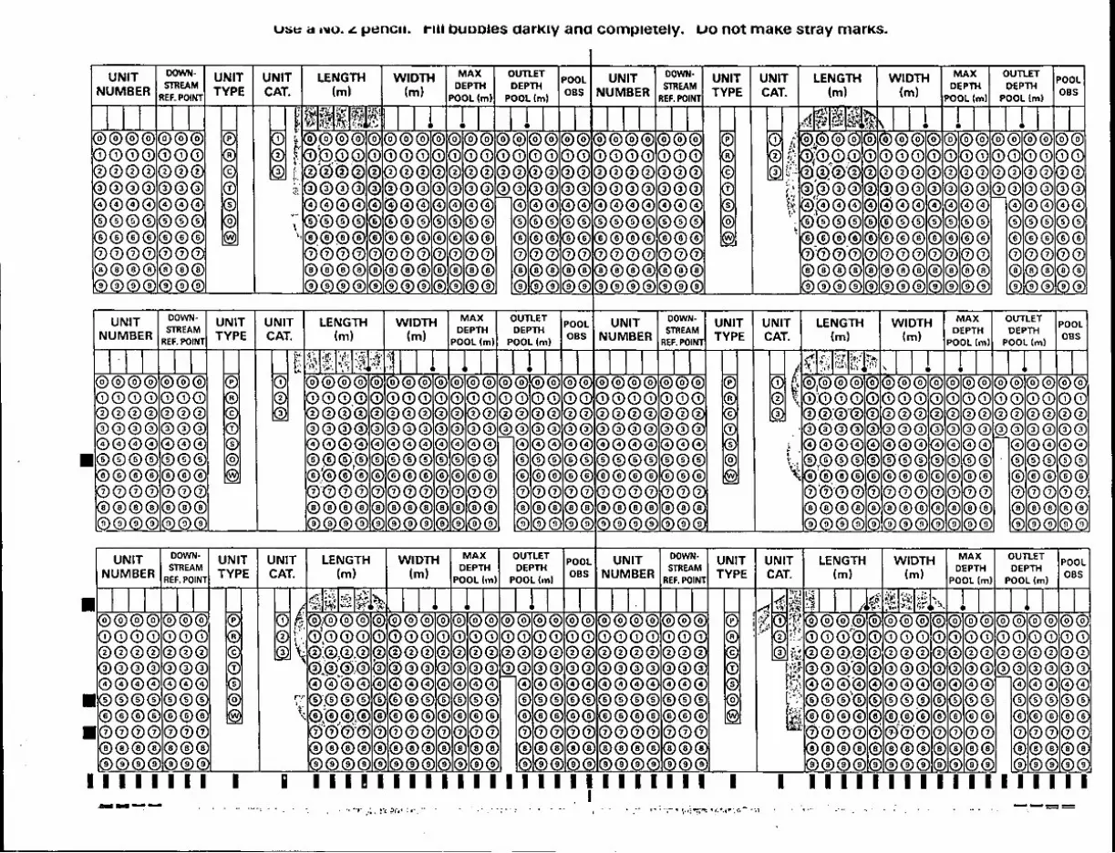
u .. t: .. '''0. "- ... ,mcl!. 1'"111 bUDDies aarKIY ana completely. L10 not maKe stray marKs.

UNIT DOWN- UNIT UNIT LENGTH WIDTH MAX OUTLET POOL UNIT DOWN- UNIT UNIT LENGTH WIDTH MAX OUTLET POOL

NUMBER R~~'~' TYPE CAT. (m) (m) Ip~~~) P~~~~) OBS NUMBER '~:'~T TYPE CAT. (m) (m) Ip~~~;~) P~~~) OBS

I I liE ~;!ltj;~J ~;! .. I J 1 I I I '" IS;:H(·, l:'~\ I I I

UNIT DOWN- UNIT

NUMBER R!':~'~' TYPE

-----

UNIT CAT.

LENGTH (m)

11i. H,'.~ IL : . )(

.. ~,:)\

WIDTH (m)

I I

, " .". ,;, ~.~ ?,',' : " ..

MAX ounET pnm UNIT DEPTH DEPTH ...........

POOL 1m) POOL (m) OBS NUMBER

I 1 I I

DOWN· STREAM

I

UNIT UNIT TYPE CAT_

I

LENGTH (m)

. .... ",

WIDTH (m)

MAX ounET IDI"'I."'I

DEPTH DEPTH 1';8"'5" POOl{m) POOl{m)

I I ~-==

To Convert;

Centigrade Fahrenheit

Centimeters

I APPENDIX E I

CONVERSIONS

Multiply BYi

(nOC * l.8) + 32 (n"F * .5556) -17.8

0.03281

To Obtain;

Fahrenheit Centigrade

Feet Centimeters 0.3937 Inches

~_SubicFe~ _____ ~.028~ _____ ~bicMae~~ Cubic Meters 35.31 Cubic Feet Decimeters 0.1 Meters

Feet 30.48 Centimeters Feet 0.3048 Meters

~ __ ye~ ______ 28,940.0 ______ ~les __ Inches 2.54 Centimeters Inches 0.0254 Meters Inches 0.02778 Yards Meters 100.0 Centimeters

~ __ Met~ _______ 3.28L _______ Fee~ __ Meters 39.37 Inches Meters 0.0006214 Miles Meters l.094 Yards

Meters/Sec 3.281 Feet/Sec 1-___ Mile1.. _______ 5..J80.Q. _______ Fe~ __

Miles 1,609.0 Meters Miles 1,760.0 Yards

Pounds 0.4536 Kilograms Yards 0.9144 Meters Yards 0.0005682 Miles

TFW Ambient Monitoring Program Code Sheet I APPENDIX F I

Habitat Unit Survey I I Large Woody Debris Survey I UnithPe

P-POOL R-RIFFLE C-CASCADE T-TAILOUT

Unit CategOlY

1 - Primary Unit (>50% wetted stream width)

2 - Secondary Unit « 50% wetted stream width)

3 - Side Channel Piece Length by Zone S - SUB-SURFACE O-OBSCURED W-WETLAND

(isolated by an island. Island = length is 2x BFW + perennial vegetation Furthest extent the piece influences:

Factors contributing to pool information

Log(s)

Rootwad(s)

Debris Jam

Roots of standing

Bedrock outcro

Channel bedform

Code

. 1

·2

3

4

5

6

7


resistant banks

8

Artificial bank

Beaverdam

Other

BFW I M' I RPD Table

* Habitat Unit Survey -Unit Identification; Lumping

and Splitting Criteria

* LWD Survey - Pool Fonning Function

9

10

11

Bankfull Width (m)

0.0 - 2.5 2.5 - 5.0 5.0 - 10.0

10.0 - 15.0 15.0 - 20.0

> 20.0

Zone 1 - W/in Wetted Channel Zone 2 - W lin Bankfull Channel Zone 3 - Above Bankfull Channel Zone 4 - Outside Bankfull Channel

Piece Stability

R - Root System B - Partially Buried (> 50% dia.) P - Pinned or Pegged

U - Unstable

Wood Type

C - Conifer D - Deciduous U - Unknown

Minimum Unit Surface Area

(m')

0.5 1.0 2.0 3.0 4.0 5.0

Y - Yes N -No

Minimum Residual Pool Depth

(m)

0.10 0.20 0.25 0.30 0.35 0.40

Northwest Indian Fisheries Commission, 6730 Martin Way E., Olympia., WA 98506 (206) 438-] 181 ext. 332 g:\manuaJ94\1wdadx.pm4

APPENDIXG TFW Ambi~nt Monitoring Stream Segment Summary 1992

Stream Segment Identification ( Fi leID: CC )

stream name, WF.:IA number:

DESCHUTES P. WAU name: WAU #, 13 .. 0028

F.:iver mile: to Segment number:

36.6

Stream Segment Characteristics

18

Gradient category: 2 CClnfinement: U Stream order, 4 Avg bankfull width: 20.2 M Segment length: 2615.0 M

Avg bankfull depth: 0.4 M Upper elevation: 550 F

Width / depth: 46.66 Lower elevation: 510 ~

Resource Condition Indice Summary

Percent pools = 51.81. rated as a GOOD ()=50X 'habitat condition In-channel LWD pieces / bankfull width = 3.11 rated unkwn target value of Average canopy closure: 23 %

Habitat Unit Summary Information

Habitat Units pel' Kilometer = 40.54

I. Total X Mean Ma:.{i mLlm Freq Total Area (W"2) T,:,tal F:PD (M) F.:PD (M)

----- ---------- ----- ------- -------Pools F:iffles Cascades Tailout

50 40 15

1

106

47.2 37.7 14.2 o. '3

18120.1 51.8 15011.7 42. '3

1748 .. 6 5.0 10'3. 1 O~3

34'38'3.4

Factors Contributing to Pool Formation

Factor Description Freq ------ -----------------------------

1 Log(s) 4 2 F~c,ot wad (s) 15 3 Debris .jam 10 4 RC'C,ts of standing trees 1:IY stumps 2 5 F.:CII: k (5) ell'" belLll del'" (5) 1 6 Bedl'" ell: k clutCl'"OP 4 7 Channel bedform 0 8 SCOUl'" associated with resistant banks 8 '3 Artificial bank

10 Beaver-11 Othe~

Subsurface flow Obscur-ed flow Wetland

Total

Dam

Freq

o o (>

o

pr-otection

Length

0.0 0.0 0.0

0.0

0 0 0

Main channel Secondayy I:h Side channel

Total

0.61 2.70

I. Area Tc,tal (M .... ··2) ----- ------

8.0 8'32.0 30.0 35'37 .. 3 20.0 3888.5 4.0 673 .. 2 2.0 51'3.1 8.0 1205a5 0.0 0.0

16.0 3371.2 0.0 0.0 0.0 0.0 0.0 0.0

Freq Length

76 2615.0 16 443. '3 14 321. 1

106 3380.0

I.Total Area

------4. '3

1'3. '3 21.5 3.7 2. ':3 6.7 0.0

18.6 0.0 0.0 0.0

Timber-fish-Wildlife Ambient Monitoring Program

LARGE WOODY DEBRIS SURVEY MODULE

August 1994

Dave Schuett-Hames Jim Ward

Martin Fox Allen Pleus Jeff Light


,.....----------------------~ .. ---


Contents


Introduction ................................................................................................................ 3

Purpose of the Large Woody Debris Survey Module ................................................... 4

Large Woody Debris Survey Methodology ................................................................. 4

Infonnation and Equipment Needed .......................................................................................... 5 IdentifYing Large Woody Debris ............................................................................................... 6 The Level I Large Woody Debris Method .. , ............................................................................... 8 The Level 2 Large Woody Debris Method .... ; ............................................................................. 9 Large Woody Debris Jams ....................................................................................................... 14

Filling Out Large Woody Debris Survey Forms ........................................................ 15

Header Infonnation .................................................................................................................. IS LWDLeve11 Fonn4.1 ............................................................................................................ 16 LWD Level 2 Fonn 4.2 ............................................................................................................ 17 LWD Jams Levell & 2 Fonn 5 ................................................................................................ 18

Data Processing and Analysis ..................................................................................... 18

Training, Field Assistance and Quality Control ......................................................... 18

References ........................................................................................ _ ...................... 19

Appendixes ............................................................................................................... 21

1994 TFW Ambient Monitoring Manual Large Woody Debris - I

Acknowledgements

Thanks to Larry Dominguez, Paul Faulds, Mark Mobbs and Mindy Rowse for comments and suggestions used in the development and refinement of this module.

Cover photograph by Allen PIeus.

1994 lFW Ambient Monitoring Manual Large Woody Debris - 2

:=i7- - -


Introduction

Large woody debris (LWD) is an important component of stream channels in the Pacific Northwest. It plays an integral role in the formation of channel morphology and fish habitat. Logs and rootwads enter stream channels due to bank cutting, blowdown, and mass wasting. Once in the channel, the effect of L WD is related to the size, stability and longevity of the individual pieces, and to the tendency of wood to collect in large accumulations known as debris jams (Figure J).

Figure I. CSS Field Tech. Joe Apfel surrounded by a large debris jam on West Fork Taneum Creek.

Large woody debris influences channel morphology in several ways. Pools often form in association with L WD, due to adjacent scouring or impoundment of water behind channel-spanning pieces. Large woody debris often traps and stores sediment, having a moderating affect on sediment transport rates. In steeper, smaller channels, it often forms distinct steps that capture sediment on the upstream side and dissipate energy as the flow drops over the step.

Large woody debris plays an important biological role in Pacific Northwest streams, creating and enhancing fish habitat in streams of all sizes (Bisson et aI., 1987). Pools formed in association with L WD often provide deep, low velocity habitat with cover. This habitat is beneficial for a variety of salmonid species and life history stages, particularly those that over-winter in stream channels. Large woody debris also functions to retain spawning gravel in high energy channels and provides thermal and physical cover.

1994 TFW Ambient Monitoring Manual Large Woody Debris - 3

The nature and abundance oflarge woody debris in a stream channel reflects past and present recruitment rates. This is largely determined by the age and composition of past and present adjacent riparian stands. Activities that disturb riparian vegetation, including timber removal in riparian areas, can reduce LWD recruitment. In addition, current conditions also reflect the past history of both natural and management-related channel disturbances, such as flood events, debris flows, splash damming, and stream clean out.

Our understanding of the function oflarge woody debris in stream channels is still developing. To help increase the state of knowledge regarding L WD distribution and characteristics in Washington streams, Peterson et al. (1992) recommend expanding the type and amount of information collected in L WD monitoring and inventory surveys.

Purpose of the Large Woody Debris Survey Module

The purpose of the large woody debris survey module is to:

1. Provide a means of accurately documenting the current abundance and characteristics of large woody debris in stream channels.

2. To provide a repeatable methodology that can be used to monitor changes in the status of large woody debris over time.

3. To provide information on the abundance, size and function oflarge woody debris that is suitable for use in the Watershed Analysis cumulative effects assessment procedure.

4. To improve our knowledge of the distribution and characteristics oflarge woody debris in Pacific Northwest streams.

Large Woody Debris Survey Methodology

This method is designed to be used in conjunction with the Stream Segment Identification and Reference Point Survey modules. Please refer to these modules if you have not completed them.

This section describes procedures for identifYing and measuring large woody debris and large debris jams. Two options are provided for collecting information on logs and rootwads. The Level I method is least intensive and does not require measurement of individual pieces of wood. It is designed to collect a minimal amount of information on L WD rather rapidly and generate information on the abundance and size class ofLWD suitable for Watershed Analysis Levell. The more intensive Level 2 method'involves taking measurements on individual pieces of wood. This method is more time consuming, however it provides detailed information on attributes such as diameter, length, volume, channel location, wood type and stability that is suitable for Watershed Analysis Level 2. Please record all measurements in metric units to reduce confusion and streamline data processing.



In order to complete the Ambient Monitoring large woody debris survey, it is necessary to have previously identified a survey segment (see stream segment identification module). It is also desirable to have established reference points (see the reference point survey module) so that large woody debris and debris jams can be associated with pennanent reference locations. You will need the following equipment:

*Fiberglass tape (metric) *Stadia rod (metric) *Calipers, Biltmore Stick, Logger's tape (metric) *Electronic or Optical rangefinders (metric) Large Woody Debris survey Fonn 4.1 or 4.2 Large Debris Jam survey Fonn 5 Number 2 pencils Clip board or fonn holder Field notebook Field guide to tree identification (to help distinguish coniferous and deciduous species) Hip boots or waders First aid supplies (* calibration required)

Calibration

Calibration of field measurement equipment is the first task before the start of the survey season, and for some types of equipment at the start of each survey day. Calibration infonnation should be recorded and a copy incorporated with your project files.

All linear measurement equipment is calibrated against a designated 50 meter fiberglass tape (a 30 meter tape will work ifit the longest or best you have). To designate your calibration standard tape, choose the newest equipment that does not have any breaks or splices for its entire length. The accuracy of the calibration standard is determined by comparing it to other tapes that are not spliced or broken. Once you have designated a fiberglass tape, identifY it as such by writing "Calibration Standard" in pennanent marker on the housing and include the date.

To calibrate other equipment to your standard, find an open area and roll out the tape in a straight line with the zero end anchored. The Large Woody Debris Survey Module has several pieces of equipment which need to be calibrated at least once per year as follows:

Fiberglass Tape: Anchor the zero ends at the same point as the calibration standard and run the tape out completely. Return to the zero end. While holding both tapes taught, proceed along the tapes and compare markings at each 0.1 meter for two meters and at each meter mark for the rest of the length. Note any damage such as breaks or splices and repair or replace them if necessary. Using a penn anent marker, write "Calibrated" on the housing of the equipment and include the date.


-....,.."....,.....,.,,.....,.,.....,.----------------------------_ ...... _.-

Stadia Rod: Place the stadia rod parallel to the calibration standard with the zero ends at the same point. Check the accuracy of the markings to the 0.01 meter level for the first 2 meters and the rest at the 0.1 meter level. Check the rod for damaged and illegible markings. Locking buttons are often replaceable if they no longer function properly. Illegible markings can be fixed by permanent marker if not too severe. Avoid using any correction factors for damaged equipment.

Log Calipers, Biltmore Sticks, Logger's tape (metric): Log calipers are checked against the calibration standard tape at the centimeter level. Also, inspect the equipment for damage or misaligned blades. Biltmore sticks and logger's tapes must be checked with similar equipment and cross-checked with the log caliper readings.

Electronic and Optical rangefinders (metric): Electronic rangefinders must be calibrated daily and optical rangefinders must be calibrated at least twice daily and more if needed. Use your calibration standard tape and check the accuracy of your instruments at 5, 15, and 30 meter intervals. Adjust instruments according to manufacturer guidelines and stated accuracy ranges.

Identifying Large Woody Debris

For the purposes of the large woody debris survey module, there are three types ofLWD; logs, rootwads and large debris jams. Somewhat different information is collected for each type, so the first step is to identifY the type of piece being observed.

How to IdentifY a Log

To qualifY as a log, a piece of wood must (Figure 2a):

1. be dead (or imminently dying with no chance of survival); 2. have a root system that is wholly or partially detached and is no longer capable of supporting

the log's weight; 3. have a diameter of at least 10 cm for at least 2 meters of its length, and; 4. intrude into the bankfull channel.

This criteria is based on the definition ofLWD used by Bilby and Ward (1989; 1991), and is compatible with the Watershed Analysis L WD assessment procedure. Pieces that meet the minimum length and diameter criteria above are classified as logs regardless of whether or not they have roots attached.

Individual stems that have grown in a cluster and meet at the base may be counted as separate pieces if they meet the minimum length and diameter criteria. Branches that are attached to the trunk of the tree should not be counted regardless of their size. Trees or logs which have been broken into smaller pieces are counted as separate if they meet minimum criteria. Use the "pick-up" technique to help determine if they are separate. To do this, imagine a crane picking-up one of the broken pieces; if the other piece did not remain attached, it would be counted separately. This technique can also be used to determine the length of an extensively rotted log or rootwad.


Take dia11etI:r ac:nm midpoint

/H,~------'-- > 2m -------------;.1

LOG Fig.2a Oiteria: 1) must be dead or death Is Immenant [NO d'Iance of survivaQ

21 roots must no longer support !he weight of !he log 3 1 Oem diameter for at least 2m length

Note: measure log length 10 bo!Iom of rootwad if al!a1Ll lEd 4) must Intrude on bankftJD dlannel

ROOTWAD Oiterta: I) roots must be detatd1ed: eIttler It has faDen CNer or It

has the abtTrtylO fall CNer

21 length less than 2 meters 3 dIameter where stem meets roots greater than 20 an 4 must intrude on bankfull channel

Fig. :2. b

Figure 2. Criteria for large woody debris.

How to IdentifY a Rootwad

<2m-~

Rootwads are pieces of wood with a root system that do not meet the minimum length criteria for a log. To qualifY as a rootwad, a piece (Figure 2b);

1. must be less than 2 meters long (except for old-growth stumps) and have a root system attached;

2. must be at least 20 cm diameter at the base of the stem where it meets the roots; 3. must have roots that are detached from their original position on the floodplain or terrace;

and/or the rootwad has the ability to fall over; and 4. must intrude into the bankfull channel.

1994 TFW Ambient MonitOring Manual Large Woody Debris - 7

Old stumps are often found along the banks of stream channels running through areas that were harvested in the past. Often the stream has cut into the bank, exposing the roots of these standing stumps. The exposed roots are within the bankfull channel, aiJd may have an influence on channel morphology. However, to maintain consistency with Bilby and Ward (1989; 1991), stumps with root systems that are still anchored in their original position on the floodplain or terrace are not counted as rootwads. This factor can be difficult to determine especially if the piece is still in an upright position and the root system is buried. If this is the case, you must determine if the piece was originally anchored at a higher level but was undercut by the stream action and eventually recruited into the bankfull channel. If you are unsure that the stump is in its original position, don't count it. If the stem (above the roots) has fallen into the bankfull channel, the root system has obviously become detached and the piece is counted.

How to IdentifY a Large Debris Jam

Large debris jams are defined as accumulations of 10 or more qualifying logs or rootwads that are in contact with one another (Figure 3). Each qualifying piece must meet the minimum size criteria ( defined above) and must intrude into Zone 1, 2 or 3. While smaller accumulations may sometimes function as debris jams, for our purposes they are not counted as "large debris jams". Only limited information is collected on individual pieces of wood in large debris jams (see section on large debris jams, below). Figure 3. Lyman Bullchild on top of a large debris jam

in the headwaters of Charley Creek, 1991

The Levell Large Woody Debris Method

The following information is collected on qualifying logs and rootwads during the Level 1 survey. This type of information is not collected for logs or rootwads that occur in accumulations of 10 or more pieces; they are treated separately as large debris jams (see the "Large Woody Debris Jams" section).

Piece Identification

Begin the survey at the downstream start of the stream segment and walk the channel, counting the number of qualifying pieces encountered. In the Level 1 L WD survey, qualifying pieces are assigned to one of the following four categories:

*Rootwad: *Small Log: *Medium Log: "Large Log:


20 cm or greater at base of stem 10-20 cm diameter at midpoint 20-50 cm diameter at midpoint greater than 50 cm diameter at midpoint

Large Woody Debris - 8

Zone Identification

Next, determine the lowest zone to which the piece intrudes into the channel. Assign the piece to either channel location zone 1 or 2 (optional zone 3). If a portion of the piece intrudes into the water at low flow, it is assigned to Zone 1. If it does not intrude into the water at low flow but would be partially submerged at bankfull flow, it would be assigned to Zone 2. See the section on length and channel location in the Level 2 LWD method (below) for a detailed discussion of the channel location zones.

Once the size category and channel location have been determined, tally the piece in the appropriate column (size category) and row (channel location zone) in the matrix on the Level 1 Form 4.1. Each piece should only be tallied once. It may be helpful to use a piece of street or logger's chalk to mark those pieces tallied to prevent missing or duplication in complex areas. At the end of the survey add up all the tally marks in each cell of the matrix and record the total at the bottom of each cell. The sum of the totals for all cells equals the count of individual pieces in the segment. Add this number to the total number ofpieces counted in large debris jams to calculate the total number ofLWD pieces surveyed.

The Level 2 Large Woody Debris Method

The following information is collected on qualifying logs and rootwads during the Level 2 survey. This type of information is not collected for logs or rootwads that occur in accumulations of 10 or more pieces; they are treated separately as large debris jams (see the "Large Woody Debris Jams" section below).

Piece Identification

Follow the procedures for identifying a log and rootwad as noted above.

Association with Reference Points

Each log or rootwad should be assigned to a 100 meter reach delineated by established reference points (see Reference Point Survey module). Locate the mid-point along the log or rootwad, and record the number of the nearest downstream reference point (Figure 4).

Diameter

Diameter information is useful in determining the relative size and volume of individual logs. Diameter (to the nearest centimeter) is measured at the mid-point along the length of each log with a caliper, Biltmore stick, Of logger's tape. A log caliper is the most versatile instrument of the three. If a log cannot be measured, for example if the water is too deep or part of th·e log is suspended above the channel, estimate the diameter and note it as such in your field notes. If the log is divided into several large branches at the mid-point, measure the diameter immediately below the point where

1994 TFW Ambient MonitOring Manual Large Woody Debris - 9

Bounda!yot segments: End ot"3" 5t<rtof"4"

Ref. PI. 12 Ref. PI. 0

AssIgn to SeQ. "3" Ref. PI. n

Midpoint of Joq between Ref. PI. 0 andl. assign

to Ref. PI. 0

AssIgn to Ref.l't. 0

Ref. PI. I

Note: Assign large woody debris to nearest downstream reference point

Figure 4. Assigning large woody debris to reference points.

Midpoint of Joq between Ref. PI. I and-:.! - assign

. to Ref. PI. I

Midpoint of Large Debris Jam between Ref. PI. I and 2

-assign to Ref. PI. I

the branches fork. The diameter of rootwads is measured on the stem just above where the roots begin.

If the piece is round, measure the diameter with the spline of the caliper parallel to the channel substrate or water surface. If the piece of wood is irregular in shape (non-circular), take a measurement at the widest and narrowest point, sum the measurements and divide by two to calculate the average diameter.

Channel Location

Information on the length of logs and rootwads is useful in determining their relative size and volume. In conjunction with the length measurement, information on the channel location of the piece is collected. The system used to describe channel location (based on Robison and Beschta, 1991) consists offour location zones or categories (Figure 5).

Zone 1 is the wetted low flow channel, defined as the area under water at the time of the survey.

Zone 2 is the area within the influence of the bankfull flow. This zone is within the perimeter of the bankfull channel and below the elevation of the water at bankfull flow (excluding areas defined as Zone 1). Zone 2 includes areas such as gravel bars that are exposed at low flow.

Zone 3 is the area directly above the bankfull channel -from the bankfull flow waterline upwards indefinitely. This zone includes pieces that extend out over the channel but are suspended above the elevation of the water at bankfull flow;

1994 TFW Ambienl Monitoring Manual Large Woody Debris - 10

ZONE 4 • all area outside

of bankfUU channel

ftoodplafn _

"INTRUSION" into Zone: any portion of stem or rootwad which breaks its plane - no mInimum length requIrement

ZONE 3 • within banl:fIJil perfmeter

• above barldiJD stage water level

ZONE;Z • within chameI filled at banldiJU stage

• above aJII'eI"Itwetted surface _----

ZONE 4 • aU <rea outside of

barldiJU channel

... ________ ~::::~~~I ZONE 1 • OJrl'ent wetted area of stream

Figure 5. Description ofLWD zones in stream channel.

Zone 4 is the area outside of the bankfull channel perimeter. This zone includes the upper banks and riparian areas not directly influenced by bankfull flows.

Collecting information on L WD pieces in Zone 1 and 2 is important because they interact with the stream during bankfull (channel-forming) flows. These pieces can play an important role in formation of pool habitat and creation of habitat diversity during these events. They also play an important role in regulating sediment transport, routing and storage and can control the abundance and distribution of spawning gravels in some stream segments. Pieces or portion of pieces in Zone 1 also provide critical cover for salmonids during summer low flows. Pieces (especially accumulations) in both Zone 1 and 2 provide critical winter refuge habitat for juvenile coho salmon during freshets.

Collecting information on portions ofLWD pieces in Zone 3, although they do not affect a stream hydraulically, can provide information on cover quality, L WD recruitment resources to the channel, and identifY key pieces which are causing debris accumulations or jams. Collecting information on portions of L WD pieces in Zone 4 is important because their size or placement often act as anchors for the portions within the bankfull channel as well as provide potential recruitment into the channel.

Measuring Lengths by Channel Location

To measure length and channel location, first determine which zones the log or footwad passes through. A variety of methods have been used by geomorphologists to establish the outer boundaries of the bankfull channel, however many require discharge records or surveying techniques. For ambient monitoring purposes, use bank form and vegetation indicators to identifY the perimeter of the bankfull channel. See the Reference Point Survey module (pages 8-9) for a detailed discussion on determining bankfull channel dimensions. Often, it is useful to identifY all the zone boundaries on the piece before taking the length measurements. A piece of chalk is useful to help mark and remember boundary locations.

To locate the boundaries of Zone 1, first identifY where the end of the piece is. In situations where this boundary of the piece is buried or extends into deep water, use your stadia rod to quickly probe for this end. Next, locate the upper boundary where Zone 1 meets Zone 2. The boundary line

1994 TFW Ambient MonitOring Manual Large Woody Debris - II

between two zones generally passes through the log at an angle and the point you are looking for is located at the furthest extent that the log influences Zone 1. Often, this point is found where the waterline last touches the bottom of the log. At this point, use your chalk to place a 90° mark on the piece to that boundary point.

The lower boundary of Zone 2 is now established and the outer boundary needs to be located. To find this point, it is necessary to determine the point on each bank that represents the high water mark at bankfull flow. Extend this line across the channel to locate where it intersects the piece you are measuring. It is helpful to use an extend stadia rod for this purpose by placing one end at the bankfull width and having your partner step back to determine when it is level. Use this to sight along to determine the furthest extent that the piece influences Zone 2. Often, this point is found where a bankfull waterline would last touch the bottom of the piece. At this point, use your chalk to place a 900 mark on the piece to that boundary point.

The lower boundary of Zone 3 is now established and the outer boundary needs to be located. To find this point, use the bankfull width point used for establishing Zone 2 and imagine a boundary line from that point straight up. Again, it is helpful to use your stadia rod to represent this line and determine where the upper Zone 3 boundary intersects the piece. Locate the furthest extent that the piece influences Zone 3 and this is often found along the top of the piece. At this point, use your chalk to place a 900 mark on the piece to that boundary point.

The lower boundary of Zone 4 is now established and the outer boundary needs to be located. This boundary is the end of the piece located on or above the floodplain/terrace. Often, locating the end of a piece in Zone 4 is difficult, too time-consuming, or too dangerous to accurately determine. In these situations, estimate the boundary and note on Form 4.2 the accuracy of the estimate (+/- .5, 1.0, 5.0 meter).

Once the zones have been determined, measure the length of the log (Figure 6) or rootwad (Figure 7) along its main stem in each of the four zones and note estimated zone lengths as needed. If part of a piece that is within Zone 1 or 2 also extends into Zone 3 or 4, measure and record the length in Zone 3 and/or 4. It is not required to count or measure pieces which intrude only into Zone 3, however, this information can be collected if desired (see below). Pieces which lay only in Zone 4 are not counted in the survey.

Extend the length measurement from the base of the attached roots, if present, to the furthest end of the log, even if the end is less than the minimum diameter. If a portion of a log is buried and the entire length cannot be determined, measure only the exposed portion of the log. When a piece of wood forks into numerous small branches, such as the branches at the top of a tree, measure to the point where the main stem is no longer distinctly larger than the branches forking off of it.

Cooperators may also want to count and measure pieces of debris that are suspended or bridged over the channel in Zone 3. To do this, also enter data for qualifYing pieces that intrude into Zone 3 but do not enter Zone 1 or 2. These pieces will not be included in the regular wood count but will be reported in a separate category. The decision on whether to count pieces in Zone 3 within a segment is made by the project leader prior to initiating the survey.


Dead snag NOT counted as L'JVD -falls aiteria because roots still SUpport Jog~ weight ~

BankliJlI \Ii1dth

Measure zone Jeng1hs to the point where the Jog first Intrudes Into the next Jowest zone

Figure 6. Assigning portions of logs to stream channel zones.

Not ax.n1ed ac:coo:!ing to aIteia

Crtteria for measuring rootwads: • detatrt1ed rootwad must Intrude

Into Zone 1 or 2

ZONE 3

Figure 7. Assigning portions of rootwads to stream channel zones.

Wood Type

ZONE 2

Logs are classified in one of three categories based on the species of tree. The three categories are Coniferous (C), Deciduous (D) or Unknown (U). This provides information on the type of material that is entering the channel and its potential longevity, since conifers resist rot and persist longer than deciduous pieces. Characteristics of the bark, wood fiber, and branching pattern can often be used to identifY the type of wood. A tree identification guide may be useful to help identifY various species. If unsure about the type of wood, enter Unknown.

Stabilizing Factors

Note if the piece has a Root system (R), is partially Buried (B), is Pinned (P), or is unstable (U). A root system is defined as having increased stability at bankfull flow due to the presence of roots or a rootball. Buried is defined as having increased stability at bankfull flow due to complete burial of either end or lateral burial of 50% or more of the piece. Pinned is defined as having increased stability at bankfull flows due to having another qualifYing L WD piece on top of it, or due to being pegged between other logs, standing trees or bedrock. A piece can have all three factors noted if present. If none of the above stability factors are present, then the piece is considered unstable.


Pool Forming Function

Note if the log or rootwad is associated with pool formation" contributing to channel scour and the impoundment of water. Use the Habitat Unit Survey module pool criteria based on a segment's average bankfull channel width for minimum surface area and residual pool depth to help determine qualifYing pools for this category (Appendix A). This includes Zone 2 pieces outside of the summer low-flow wetted perimeter that you determine contribute to pool formation at bankfull flows.

Orientation and Decay Class

Collection of this information is optional. The classification systems listed below are not currently being trained or part of the quality assurance testing.

For Orientation, see Robison and Beschta (1990) for a more detailed description of this method. The orientation method used ("0· - 180·"; or "0·, 90·, 180") must accompany any data entered into the TFW Ambient Monitoring database.

There are two Decay classification systems recommended by the TFW Ambient Monitoring Program. These are a five-class system by Robison and a seven-class system by Grette (Appendix B). Other classification systems are acceptable. The classification method or a concise definition of the method. used must accompany any data entered into the TFW· Ambient Monitoring database.

Large Woody Debris Jams

Large woody debris jams consist of accumulations of ten or more qualifYing pieces (either logs or rootwads) that are touching. Pieces must be wholly or partially within Zones I or 2 (Zone 3 optional) to be counted in LWD jams. This information is used in both Levelland Level 2 LWD surveys.

The following information is collected on logs and rootwads that are found in L WD jams. Walking on top of L WD jams can be difficult and dangerous, so this information is intended to be collected while walking around the outside of the jam and does not necessitate actual measurement of individual pieces of wood.

Associating Large Debris Jams with Reference Points

Each debris jam should be associated with a 100 meter reach delineated by established reference points (see the Reference Point Survey Module). Locate the mid-point along the length of the debris jam, and record the number of the nearest downstream reference point (see Figure 5).

Number and Size of Visible Pieces

Walk around the debris jam and count the visible pieces that meet the minimum size criteria for logs and rootwads. Because it is often not possible to see both ends of logs that go through the middle of large jams, it may be difficult to know if you are counting the same piece twice. Using chalk to


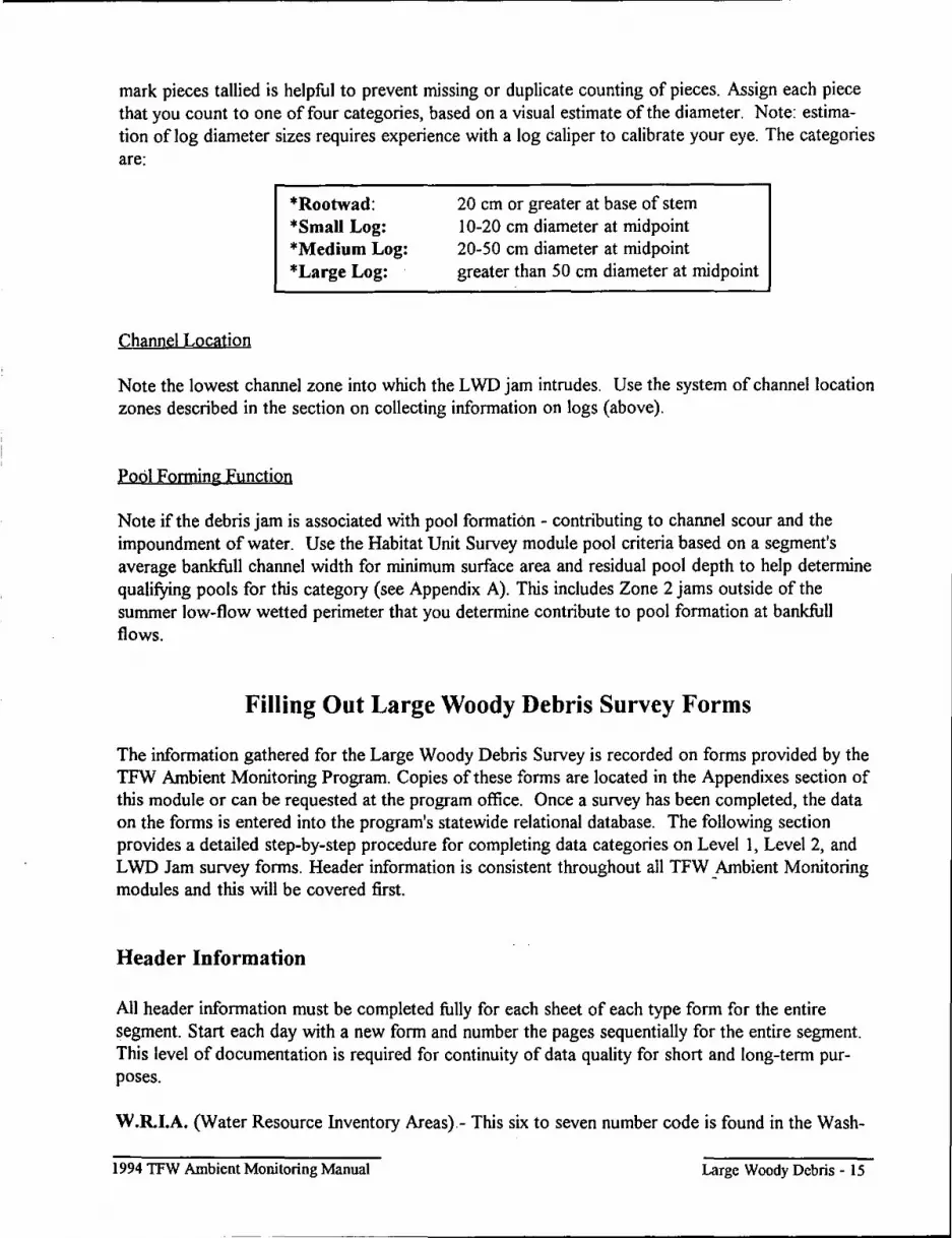
mark pieces tallied is helpful to prevent missing or duplicate counting of pieces. Assign each piece that you count to one of four categories, based on a visual estimate of the diameter. Note: estimation of log diameter sizes requires experience with a log caliper to calibrate your eye. The categories are:

Channel Location

*Rootwad: *Small Log: *Medium Log: *Large Log:

20 cm or greater at base of stem 10-20 cm diameter at midpoint 20-50 cm diameter at midpoint greater than 50 cm diameter at midpoint

Note the lowest channel zone into which the LWD jam intrudes. Use the system of channel location zones described in the section on collecting information on logs (above).

Pool Fonning Function

Note if the debris jam is associated with pool formation - contributing to channel scour and the impoundment of water. Use the Habitat Unit Survey module pool criteria based on a segment's average bankfull channel width for minimum surface area and residual pool depth to help determine qualifYing pools for this category (see Appendix A). This includes Zone 2 jams outside of the summer low-flow wetted perimeter that you determine contribute to pool formation at bankfull flows.

Filling Out Large Woody Debris Survey Forms

The information gathered for the Large Woody Debris Survey is recorded on forms provided by the TFW Ambient Monitoring Program. Copies of these forms are located in the Appendixes section of this module or can be requested at the program office. Once a survey has been completed, the data on the forms is entered into the program's statewide relational database. The following section provides a detailed step-by-step procedure for completing data categories on Level I, Level 2, and LWD Jam survey forms. Header information is consistent throughout all TFW _Ambient Monitoring modules and this will be covered first.

Header Information

All header information must be completed fully for each sheet of each type form for the entire segment. Start each day with a new form and number the pages sequentially for the entire segment. This level of documentation is required for continuity of data quality for short and long-term purposes.

W.R.I.A. (Water Resource Inventory Areas).- This six to seven number code is found in the Wash-


ington Department of Fisheries Stream catalog. Refer to the Stream Segment Identification module (page 9) for determining an unlisted number.

Segment # (Segment Number) - Record the segment number of the stream reach you are conducting the LWD survey on.

Survey Start Date - Record the date of the first day you begin this survey. This date does not change from form to form.

Survey End Date - Record the date of the last day of this survey. This date reflects all field gathering and error-checking activities up to entering the data into the database.

Stream Name - Record the official stream name (W.RI.A. designated) and any local names (in Notes section).

Basin Name - Record the basin name as stated in the W.R.I.A catalog. If your stream is in W.R.I.A 25 or greater, or you cannot find the official basin name, leave blank and the database will fill it in for you.

Rivermile from _ to _ - Record the segment's beginning (downstream) and ending (upstream) boundary rivermile location according to the W.R.I.A catalog.

Ref. PI. from _ to _ (Reference Point number) - Record the segment's beginning (usually "0") and ending reference point numbers. Use your segment's completed Reference Point Survey Form 2 for this information.

Crew LeadIRecorderl Affiliation - Record the full names of the survey crew and each person's Tribal, agency, or other work affiliation. This information is important when there are questions regarding past data that only a survey crew member might be able to answer.

Survey Date - Record the actual day that this form is being used. Each new day requires starting with a new form.

Discbarge _._CMS (cubic meters per second)/Discbarge Date - Record your most recent discharge measurment in cubic meters per second and the month/day/year taken from your Form 7 (see Habitat Unit Survey module).

LWD Levell Form 4.1

The TFW Ambient Monitoring Program provides field forms for recording monitoring data. For the Levell LWD survey, use Form 4.1 (Appendix C). There are no scan-able forms available for this level of survey. All data must be entered by hand into the database. The following section describes how to record data on this form.

Category and Zone Tally - Assign one tally-mark for each qualifYing L WD piece to one of eight (8) Category/Zone combinations (12 combinations if you are collecting Zone 3 information).


.. _------------------------------------'

Add the tally marks together at the end of the segment survey and record the number in the small "Total" box located in the lower-center portion of the tally boxes.

LWD Level 2 Form 4.2

Two options are available for recording information collected on large debris jams. Use the regular Large Woody Debris Survey Form 4.2 (Appendix D) if you plan on entering data by hand into the database. Use the scan-able version Form 4 (Appendix E) if you want to scan the data directly into the database·by NWIFC. Scan-able forms are available from NWIFC. The following section describes how to record data on the hand-entry Form 4.2.

Piece # (piece number) - Assign each qualifYing LWD piece a unique piece number, beginning with 001 and continuing sequentially to the last piece in the stream segment. Fill-out one row on the Form 4.2 for each qualifYing piece of wood (except those in LWD jams).

Dwn RefPt # (Downstream reference point number) - Record the number of the nearest downstream reference point using the mid-point of the log or rootwad.

Piece Type L-R - Record (L) for Log or (R) for Rootwad in the piece type column.

Piece Dia cm (piece Diameter in centimeters) - Record the diameter measurement (to the nearest centimeter) in the diameter column. Document estimated measurements due to buried or obstructed pieces in the Notes section.

Length - The form has separate columns for each of the channel location zones. Record the length of the portion of the log or rootwad assigned to each zone in the appropriate column. If there is no length in one or more of the zones, place a diagonal mark across that box documenting that you did not simply forget a length. Lengths are measured to the nearest 0.1 meter unless estimated and documented in the Notes section. Total lengths and volumes are computed during data processing.

Wood type - Record the type of wood in this column using (C) for Conifer, (D) for Deciduous or (U) for Unknown.

Stability - Use this column to record all of the applicable stability factors for tIle piece using (R) for Root system, (B) for Buried, (P) for Pinned, and (U) for Unstable.

PFF (pool Forming Function) - After determining if the log or rootwad is associated with a pool, use this column to record (Y) for Yes and (N) for No.

Orientation - Optional. Use this column to record the angle of orientation of the piece in the bankfull channel (0° - 180°; or 0°, 90°, or 180°). Document in Notes section which method is being used on the first form of the survey.

Decay - Optional. Use this column to record the number or letter code relating to the method used. Document in Notes section which method is being used on the first form of the survey.


LWD Jams Levell & 2 Form 5

Two options are available for recording information collected on large debris jams. Use the regular Large Woody Debris Jam Survey Form 5 (Appendix F) if you plan on entering data by hand into the database. Use the scan-able version Form 5 (Appendix G) if you want to scan the data directly into the database by NWIFC. Scan-able forms are available from NWIFC. The following section describes how to record data on this form.

Jam # (LWD jam number) - Assign each LWD jam in the segment a unique number beginning with 001 and sequentially numbering each jam to the end of the segment. Fill-out one row of Form 5 for each qualifying LWD jam (10 or more interconnected qualifYing pieces of wood).

Dwn RefPt # (Downstream reference point number) - Record the number of the nearest downstream reference point using the mid-point along the length of the LWD jam.

Visible pieces - Tally the total number of visible pieces in each of the size categories in the appropriate column, add the tally marks together at the end of the survey and record the number in the small box located in the lower-right-hand corner of the tally boxes.

Zone (Jam channel location zone) - Record the zone number (I, 2, or optional 3) documenting the lowest zone the L WD j am intrudes into the bankfull channel.

PFF (pool Forming Function) - After determining if the jam is associated with a pool, use this column to record (Y) for Yes or (N) for No.


After data has been hand entered (by the cooperator) or scanned into the database, it is error checked. Then, an in-channel Large Woody Debris summary report is generated (Appendix H). This report provides information on LWD for the segment including: the frequency, average diameter, length and volume by channel location zone ofiogs and rootwads; frequency and volume by species type; and the size and composition of debris jams. This information is suitable for use in Watershed Analysis or for assessment and monitoring purposes. In addition, cooperators will receive a copy of the database on floppy disk for their use. Data is stored in a statewide database at NWIFC for future TFW -related use.


This manual is intended as a reference for those collecting information using the TFW Ambient Monitoring Program Large Woody Debris Survey Module. Because of the difficulty in relying solely on a manual to learn and implement monitoring methodologies, the TFW Ambient Monitoring Program offers formal training sessions and informal field assistance visits to help cooperators learn and implement the methodologies.


In addition, the Ambient Monitoring Program also provides a quality control service that uses an experienced crew to perform replicate surveys for cooperators. The purpose of these replicate surveys is to identifY and correct inconsistencies in application of the methods and to provide documentation that data is being collected in a replicable and consistent manner throughout the state. The quality assurance service entails both pre- and mid-season QA surveys. The pre-season QA survey documents that your crews are collecting high quality data from day one. The mid-season QA survey documents crew consistency and whether training or corrections applied to problems during the first QA survey were effective. For more information on quality assurance protocols, refer to the Quality Assurance Module. .

We encourage cooperators to utilize these services. Please contact the Northwest Indian Fisheries Commission (1-206-438-1181 ext. 332) for more information concerning the TFW Ambient Monitoring Program.

References

Bilby, RE. and J.W. Ward. 1989. Changes in characteristics and function of woody debris with increasing size of streams in western Washington. Trans. Amer. Fish. Soc. 118:368-378.

Bilby, RE. and J.W. Ward. 1991. Characteristics and function oflarge woody debris in streams draining old-growth, c1earcut and second growth forests in southwestern Washington. Can. J Fish. Aquat. Sci. 48:2499-2508.

Bisson, PA, RE. Bilby, M.D. Bryant, c.A. Dolloff, G.B. Grette, RA. House, M.L. Murphy, K.Y. Koski and JR Sedell. 1987. Large woody debris in forested streams in the Pacific Northwest: past, present and future. Pages 143-190 IN' E.O. Salo and T. Cundy (eds.). Streamside management: forestry and fishery interactions. College of For. Res. Univ. of Wash. Seattle.

Peterson, N.P., A. Hendry and T.P. Quinn. 1992. Assessment of cumulative effects on salmonid habitat: some suggested parameters and target conditions. Center for Streamside Studies. Univ. of Wash. Seattle.

Robison, E.G. and R.L. Beschta. 1990. Characteristics of coarse woody debris for several coastal streams of southeast Alaska, USA. Can. J Fish. Aquat. Sci. 47:1684-1693.



APPENDIXES

Appendix A HabitatILWD Code Sheet

Appendix B Decay Class Codes

Appendix C LWD Level IForm 4.1 - Hand entry

Appendix D LWD Level 2 Form 4.2 - Hand entry

Appendix E LWD Level 2 Form 4 - Scan entry

Appendix F LWD Jam Form 5 - Hand entry

Appendix G LWD Jam Form 5 - Scan entry

Appendix H LWD Summary Report - example


TFW Ambient Monitoring Program Code Sheet APPENDIX A I

I Habitat Unit Survey I Unit Type

P-POOL R-RJFFLE C-CASCADE T-TAILOUT

Unit Category

1 - Primary Unit (>50% wetted stream width)

2 - Secondary Unit « 50% wetted stream width)

3 - Side Channel

I Large Woody Debris Survey

Piece Length by Zone S - SUB-SURFACE O-OBSCURED W-WETLAND

(isolated by an island. Island = length is 2x BFW + perennial vegetation Furthest extent the piece influences:

Factors contributing to pool infonnation

Log(s)

Rootwad(s)

Debris Jam

Roots of standing

Bedrock outcro

Channel bedfonn


resistant banks

Artificial bank

Beaver dam

Other

Code

. 1

3

4

5

6

7

8

9

10

11

BFW I W I RPD Table Bankfull Width

* Habitat Unit Survey -Unit Identification; Lumping

and Splitting Criteria

* LWD Survey - Pool Forming Function

(m)

0.0 - 2.5 2.5 - 5.0 5.0 - 10.0

10.0 - 15.0 15.0 - 20.0

> 20.0

Zone 1 - Wlin Wetted Channel Zone 2 - W/in Bankfull Channel Zone 3 - Above Bankfull Channel Zone 4 - Outside Bankfull Channel

Piece Stability

R - Root System B - Partially Buried (> 50% dia.) P - Pinned or Pegged

U - Unstable

Wood Type

C - Conifer D - Deciduous U - Unknown

Minimum Unit Surface Area

(m')

0.5 1.0 2.0 3.0 4.0 5.0

Y - Yes N-No

Minimum Residual Pool Depth

(m)

0.10 0.20 0.25 0.30 0.35 0.40

Northwest Indian Fisheries Conurussion. 6730 Martin Way E .. Olympia, WA 98506 (206) 438·1181 ext. 332 g:\manuaI94\1wdadx.pm4

APPENDIXB

Decay Class Methods usable with the TFW Ambient Monitoring Program Large Woody Debris Level 2 Survey.

Robison and Beschta (1991)

TABLE 2. A five-class system of evaluating de,cay of coniferous aquatic coarse woody debris, adapled from Maser and Trappe (I984):if .

Decay class

I

2

:3

;-

Grette (1985)

Class

1 2 3 4 5 6 7

Twigs Bar\:: (3 cm; 1.18 in) Te.lUre Shape

iniaC! Preseot iniaC! Round

IniaC! Absenl iniaC! Round

Trace Absenl Smooth; Round some surface abrasion

Absent Absenl Abrasion; Round 10 some holes oval and openings

Absenl Absenl Vesicular; Irregular many holes and openings

*··M.~ER. C:. ANI?J: M. TRApPe. 11'EcH. ED.). 1984. The seen and unseen world of the rallen tree. USDA For. Servo (}en. Tech. Rep. PNW-I64. S6 p.

Description

bark intact, limbs present bark intact, limbs absent bark loose or absent bark absent, surface slightly rotted surface extensively rotted surface rotted, center solid surface rotted, center rotted

Northwesl Indian Fisheries Conunission, 6730 Martin Way E .. Olympia, WA 98506 (206)438-1 t 81 ,,1. 332

Wood coJor

Original coJor

Original color

Origial color; darkening

Dar\::

Dar\::

g:lmanuaI94Uwdapx2.pm4

~---------

Form TFW Ambient

W.R.LA. --'-----'---LARGE WOODY DEBRIS SURVEY I Segment # OLB ORB

Stream Name Basin Name Rivermile from Ref. Pt. from

___ to __ _ to I LEVEL 1 I

Survey Start Date _ I _ I __ Survey End Date _ 1_ 1 __ Fill out aU' icl-~ti~ on every form. Full

names required on rust form for each day· initials can be used on secondary pages

Crew Lead Recorder

AffiIiation Survey Date _. _,_, __

ROOTWAD >20em

LOG 10 - 20 em

Total

Total

Northwest Indian Fisheries Commission, 6730 Martin Way E., Olympia, W A 98:506 (206) 438·1180

LOG 20 - 50 em

.... - -- -_._ ....

: Total

Total

Discharge __ . _ eMS Discharge Date I I

LOG >50em

.. Total

Northwest tndian Fisheries Commission. 6730 Martin Way E., OI)111pia. WA 98506 (206) 438.1180

« o


LARGE WOODY DEBRIS SURVEY I W.R.LA. . . -- ----- ---Segment # OLB ORB


___ 10 __ _

10 I LEVEL 2 I Survey Start Date _, _, __ Survey End Date _ ,_, __ Fill out all information on every fann. Full

names required on first fann for each day· initials can be used on secondary pages

Crew Lead . Recorder

Affiliation Survey Date _,_, __

Own Piece Piece

Piece Type Dia L·R em

Length Wood Type

Zone 1 Zone 2 Zone 3 Zone 4 C·D· U

I Discharge --' - CMS I Discharge Date _,_, __

Notes

'=r--1---r---r--+-~~-+--~--+---4----+~~---+--~----------------~ ~ .: Et---~-_+--_+--+_--~--_4----~---+_---_+----+_~-~---4_----_4r_--------------------~

~ ~r---~----_+----~----+_--_4~--_+----4_----+_---~-----+_~_4~----+_----~----------~-------------~

~ ;;: « r---~---_+----_r---+_--~r_--_+----4_----+_----~-----+_~_4~---+_----~-------------------------~

Northwest Indian Fisheries Commission, 6730 Martin Way E., Olympia. WA 98S06 (206) 438-1180 g:\manuaI94\fonn4-2.pm4

«

" ·c

~ .S

«

Field Form TFW •

Dmt Piece Piece Length Wood Piece IRe~PI Type Dia Type

# L·' em Zone I Zone 2 Zone 3 Zone 4 C·D·U

.

Northwest indian Fishenes CommISsIon. 6730 Martin Way E., Olympia. WA 98506 (206) 438-1180

FORM 4.2 (cont.)

1,,- ~.- ."

~-Notes -.

R·B·P·U

i I I I

,

I

I ! I ! I

I I

i i I

! I I

g:\rnanuaI94\fonn4-2.pm4


LARGE WOODY DEBRIS SURVEY LEVEL II


STREAM NAME

PIECE DOWNSTREAM NUMBER REF.PT.

I I I I I ®®®® ®®® 0000 000 ®®®® ®®® ®®®® ®®® 0000 000 ®®®® ®®® ®®®® ®®® 0000 000 ®®®® ®®® ®®®® ®®®

PIECE TYPE

©®

BEGINNING ENDING CONF.I DATE RIVER MILE RIVER MILE GRAD.

MO. DAY

I I ! I I ®~ ®® 00 00 ®® ®® ®® ®® 00 00 ®® ®® ®® ®® 00 00 ®® ®® ®® ®®

DIAMETER (CM)

LENGTH (METERS)

1 2 3

I I I ! 1 ! I ! ®®® ®®® ®®® ®®® 000 000 000 000

, ®®® ®®® ®®® ®®® ®®® ®®® ®®® ®®® 000 ®®® ®®®

000 000 000 ~®® ®®® ®®® ®®® ®®® ®®®

000 000 000 000 ®®® ®®® ®®® ®®® ®®® ®®® ®®® ®®®

DISCHARGE

YA. (OPT.)

I I I ! I ®® ®®® ®® 00 000 00 ®® ®®® ®® ®® ®®® ®® 00 000 00 ®® ®®® ®® ®® ®®® ®® 00 000 00 ®® ®®

®®® ®® ®®® ®®

WOOD TYPE

4

I ! I@@@I

®®® 000 ®®® ®®® 000 ®®® ®®® 000 ®®® ®®®

00 ®® ®® 00 ®® ®® 00 ®® ®®

... : ." '-" .-.'-- .:.- ----"

FORM 4

Page __ 01. __

W.R.I.A. NUMBER

00000 ®®®®® ®®®®® 00000 ®®®®® ®®®®® 00000 ®®®®® ®®®®®

STABILITY FACTOR

L®®®@.>I

> l® 00 lod 10 ®® lod )® ®® ~ )® 00 ~ )0 ®® l® ®® ~ I® 00 10 ®® ~ I® ®®~~::'J®

POOL FORMING FUNCTION

@@

•

. ~ . . . . . -. . . . . . . . . . . . . . . .- . . . . . . . . . . . . . . . ~ , . . . . . . . . . ~ . . . . . . . . . . . .

... : ..... , .. ' .. ' -.. . ... .. --~~ . I

I I I I I I I I I I I I I I I I I I I I I I I I I I I I I I I I I I I I I I I I I I I I I I I I I I I I I I I I I I I I I I I ®®® ®®® ®®® ®®® ®®®

®0 NOIJ.::)Nn~

~NIIIIHO~

100d

®0 NOIJ.:JNn~

~NIIIIHO~

100d

NOIJ.:JNn~

~NIWHO~

100d

I@@®®I

HOJ.:JIf~

AJ.I1181fJ.S

J®@®@1 HOJ.:JIf~

AJ.1118lfJ.S

HOJ.:JIf~

AJ.I1I 8 If J.S

I@@@I

3dAJ. OOOM

I@@@I

3dAJ. OOOM

3dAJ. OOOM

®®® 000 ®®® ®®® 000 ®®® ®®® (i)(i)(i) @@@ i , ~

®®® ®®® 000 ®®® ®®® 000 ®®® ®®® (i)(i)(i) @@@ i , ~

®®® ®®® 000 ®@® ®®® 000 ®®® ®®® (i)(i)(i) @@@

il ~

®®® ®®® ®®® 000 000 000 ®®® ®®® ®®® ®®® ®®® ®®® 000 000 000 ®®® ®®® ®®® ®®® ®®® ®®® (i)(i)(i) (i)(i)(i) (i)(i)(i) @@@ @@@ @@@ i , i , i ,

E ~ ~

(SH3J.3i'11) HJ.~N3l

®®@ @®® ®®® ®®® ®®® ®®® 000 000 000 ®®® ®®® ®®® ®®® ®®® ®®® 0®0 000 000 ®®® ®®® ®®® ®®® ®®® ®®® (i)(i)(i) (i)(i)(i) (i)(i)(i) @@@ @@@ @@@

i1 i , jJ E ~ ~

(SH3J.3I11) HmN3l

®®® ®®® ®<,?~ ®®® ®®® ®®® @00 000 000 ®®® ®®® ®@@ ®®® ®®® ®®® 000 000 000 ®®® ®®® ®®® ®®® ®®® ®®® (i)(i)(i) (i)(i)(i) (i)(i)(i) @@@ @@@ @@@ i , i , i ,

E ~ ~

(SH3J.3W) Hl~N3l

®®® 000 ®®® ®®® 000 ®®® ®®® (i)(i)(i) @@@

" (III:J) H3J.3111lfiO

®®® ®®® 000 ®®@ ®®® 000 ®®® ®®® (i)(i)(i) @@@

11 (III:J)

H3J.3111lfiO

®®® ®®® 000 ®®® ®®® 000 ®®® ®®® (i)(i)(i) @@@

II (W:J)

H313WlfIQ

®G:l 3dAl 3:J31d

®G:l .3dAJ. 3:J31d

3dAJ. 3:J31d

®®® ®®® 00@ ®®® ®®® 000 ®®® ®®® (i)(i)(i) @@@

11 Old O~3~

W\f3~J.SNI"Oa

®®® ®®® 000 ®®® ®®® 000 ®®® ®®® (i)(i)(i) @®@

II °J.d O~3~

W\f3~J.SNMoa

®®® ®®® 000 ®@® ®®® 00® ®®® ®®® (i)(i)(i) @@@

11 Old O~3~

!w\f3~J.SNMOa

®®®® ®®®® 0000 ®®®® ®®®® 0000 ®®®® ®®®® (i)(i)(i)(i) @@@@

'" H38wnN 3:J31d

®®®® ®®®® 0000 ®®®® ®®®® 0000 ®®®® ®®®® (i)(i)(i)(i) @@@@

'" H38111nN 3:J31d

®®®® ®®®® 0000 ®®®® ®®®® 0000 ®®®® ®®®® (i)(i)(i)(i) @@@@

"' H38wnN 3:J31d

• •

•

•


Segment # OLB ORB LARGE WOODY DEBRIS SURVEY I W.R.I.A. --'-----'---


Crew Lead Recorder

Jam Own

RefPt

___ to to

Rtwds > 20 em

Survey Start Date _,_, __ Survey End Date _,_, __

I LARGE DEBRIS JAMS IL-------------I Fill out all information on every fann. Full names required on fim rann for each day·

initials can be used on secondary pages

Affiliation Survey Date _' _1_1 __

Visible Pieces

10 - 20 em 20 - 50 em >50 em Zone 1 - 3

I Discharge ' __ ._CMS I Discharge Date _,_, __

Notes

« U

'1: ~r---+---~----L--+----~--+---~--~----~--~-4-+-+--------------~

.S Er---+------t------~----~-------L----4_-------L----+_-------L----~----~~_4------------------------~ E e " 5r-----~----~r_-----L---_+------~L---_+------~----~-------L----4_----+_-L--~----------------------~

::E ~ • r-----t------r------~--~------~----~------~--~------~----~----+__r~----------------------_1

Northwest Indian Fisheries Commission. 6730 Martin Way E., Olympia., WA 98:506 (206) 438·1180 g:Imanua194Iform5,pm4

n. ,~~, Field Form TFW Ambient ,,,' FORM 5 (cont.)

Zone PFF

Notes Y!N Logs> 50 em 1·3

!)oM,

Visible Pieces Jam RefPt

# # Rtwds> 20 em Logs 10 - 20 em Logs 20 - 50 em

i I I

i ' I I

«

I 1 I ()

'5 " ::E ,S I l I ~

I

I I I

" " E " j I I ~

" ~ " I 0)

::E :;: I I I I ! «

i \ \ \ I I

i I I I I I !

I I I I i , !

,

Northwest Iftdian Fisheries Commission, 6730 Martin Way E., Olympia, WA 98~06 (206) 438~1 180


LARGE LOG JAM SURVEY LEVEL II


STREAM NAME DATE CONF.I GRAD. I .~~~ .. ~ I MO. DAY YR.

I I I I . I I I I I I I I I I I I _ LOG JAM

NUMBER

DOWNSTREAM REF. PT.

LENGTH WIDTH HEIGHT (METERS)

VISIBLE PIECES & ROOT WADS VISIBLE PIECES ROOT WADS

10-20 CM 20-50 CM >50CM >20CM

I I I I I I I I I I I I I ! I ! I ! ®®® 000

®®® 000

®®®® ®®® ®®® 0000 000 000

®®® ®®~ ®®® ®®® 000 000 000 000

®®® ®®® ®®® ®®® ®®® ®®® ®®®® ®®® ®®® ®®® ®®® ®®® ®®® ®®® ®®® ®®®® ®®® ®®® 000 000 000 000 000 000 (i)000 000 000 000 ®®® 000 ®®®

000 (i)®® 000 (i)(i)(i)

0000 000 000 (i)(i)®(i) (i)(i)(i) ~(i)(i) 0000 000 000 (i)(i)(i)(i) (i)(i)(i) (i)(i)(i)

000 000 ®00 0®0 ®®® ®®® ®(i)® ®®® @00 000 000 000 ®®® (i)(i)(i) (i)(i)(i) (i)(i)(i)

®®® ®®® ®®® ®®® ®®® ®®® ®®®® ®®® ®®®

LOG JAM

NUMBER

DOWNSTREAM REF. PT.

LENGTH WIDTH HEIGHT (METERS)


10-20 CM 20-50 CM >50CM >20CM

I I I I I I , I I I J U Il! I ! I ! ®®® ®®® ®®® ®®® ®®® ®®® ®®®® ®®® ®®® 000 000 000 000 000 000 0000 000 000 ®®0 ®®® ®®® ®®® ®®® ®®® ®®®® ®®® ®®® ®®® ®®® ®®® ®®® ®®® ®®® ®®®® ®®® ®®® 000 000 000 000 000 000 0000 000 000 000 000 0®0 0®0 00® 000 00(i)0 000 000 ®®® 000 (i)(i)(i)

®®(i) 000 (i)(i)(i)

(i)(i)®® ®®(i) ®®® 0000 000 ~00 (i)(i)(i)(i) (i)(i)(i) (i)(i)(i)

(i)(i)® (i)(i)(i) (i)(i)(i) (i)(i)(i) 000 000 000 000 (i)(i)(i) (i)(i)(i) (i)(i)(i) (i)(i)(i)

®®(i) ®®® ®®® ®®® ®®® ®®® ®®®® ®®® ®®®

BEGINNING RIVER MILE

I I !

FORMS

Page __ 01 __

ENDING RIVER MILE

I I ! DISCHARGE

I I ! I

POOL ZONE FORMING

FUNCTION

10®®@1 0®

• • - - - - - • - _ • • - ~ • _ • • • • ~ ~ • .• ~ w • • • • ~ ~ • • • • • • _ • • • • • • • • • • • • • • • • • • • • • • • •

•

•

• •

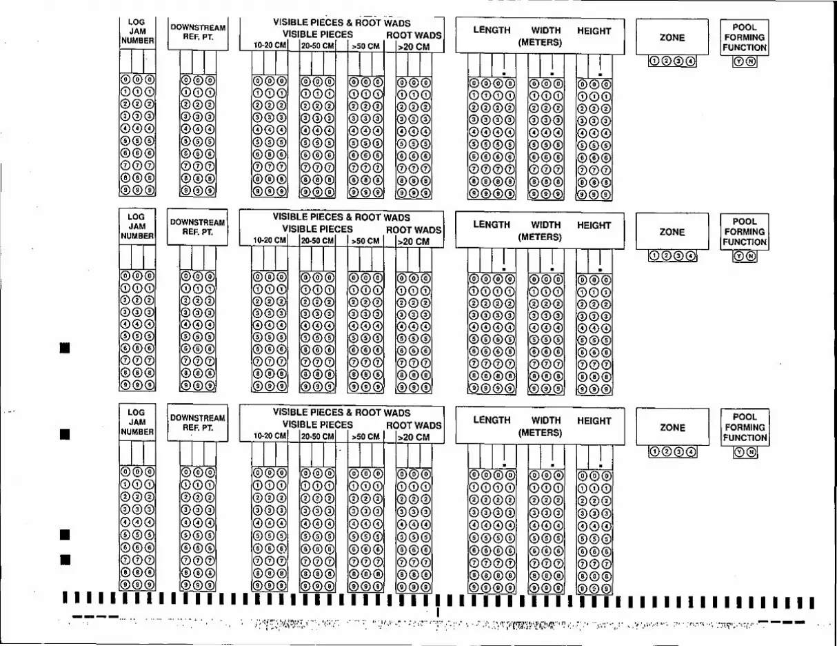
LOG JAM

NUMBER DOWNSTREAM

REF. PT.

@®® ®@® 000 000 ®®® ®®® ®®® ®®® @@@ @@@ ®®® ®®® ®®® ®®® 000 000 ®®® ®®® ®®® ®®®

LOG JAM

NUMBER

DOWNSTREAM REF. PT.

1 1 1 1 ®®® ®®® 000 000 ®®® ®®® ®®® ®®® @@@ @0@ ®®® ®®® ®®® ®®® 000 000 ®®® ®®® ®®® ®®®

DOWNSTREAM REF. PT.

LOG JAM

NUMBER

J I 1 1 ®®® ®@® 000 000 ®®® ®®® ®®® ®®® 000 00@ ®®® ®®® ®®® ®®® 000 000 ®®® ®®® ®®® ®®®

--- ---- -VISIBLE PIECES & ROOT WADS

VISIBLE PIECES ROOT WADS 10-20 CM 20-50 CM >SOCM >20CM

I I 1J 1 1 I I ®@@ ®@@ @®® ®@@ 000 000 000 000 ®®® ®®® ®®® ®®® ®®® ®®® ®®® ®®® @0@ @00 0@@ @0@ ®®® ®®® ®®® ®®® ®®® ®®® ®®® ®®® 000 000 000 000 ®®® ®®® ®®® ®®® ®®® ®®® ®®® ®®®


10-20 eM 20-50 eM >50CM >20CM

1 1 11 1 1 1 1 ®@® ®®® ®®® ®@® 000 000 000 000 0®® ®®® ®®® ®®® ®®® ®®® ®®® ®®® @0@ @00 @@@ @00 ®®® ®®® ®®® ®®® ®®® ®®® ®®® ®®® 000 000 000 000 ®®® ®®® ®®® ®®® ®®® ®®® ®®® ®®®


10-20 eM 20·50 eM >SOCM >20CM

1 1 11 1 1 1 1 ®®® ®®® @®® ®®@ 000 000 000 000 ®®® ®®® ®®® ®®® ®®® ®®® ®®® ®®® 000 @00 000 @00 ®®® ®®® ®®® ®®® ®®® ®®® ®®® ®®® 000 000 000 000 ®®® ®®® ®®® ®®® ®®® ®®® ®®® ®®®

LENGTH WIDTH (METERS)

111 I ! ®®®® ®®® 0000 000 ®®®® ®®® ®®®® ®®® @@00 @@@ ®®®® ®®® ®®®® ®®® ®000 000 ®®®® ®®® ®®®® ®®®


11 ! 1 ! ®®®® ®®® 0000 000 ®®®® ®®® ®®®® ®®® @@00 0@@ ®®®® ®®® ®®®® ®®® 0000 000 ®®®® ®®® ®®®® m®®


11 ! 1 ! ®®®® ®®® 0000 000 ®®®® ®®® ®®®® ®®® 0®@0 000 ®®®® ®®® ®®®® ®®® 0000 000 ®®®® ®®® ®®®® ®®®

HEIGHT

1 ! ®®® 000 ®®® ®®® @@@ ®®® ®®® 000 ®®® ®®®

HEIGHT

1 ! ®®® 000 ®®® ®®® @00 ®®® ®®® 000 ®®® ®®®

HEIGHT

1 ! ®®@ 000 ®®® ®®® 00@ ®®® ®®® 000 ®®® ®@®

ZONE

10®®01

POOL FORMING FUNCTION

0®

POOL ZONE FORMING

FUNCTION

100(3)(4)1 0 ®

POOL ZONE FORMING

FUNCTION

10®®01 0®

· .. ~ -.: .... ' .'; .... : .. ,. . , ...

, .. . .....

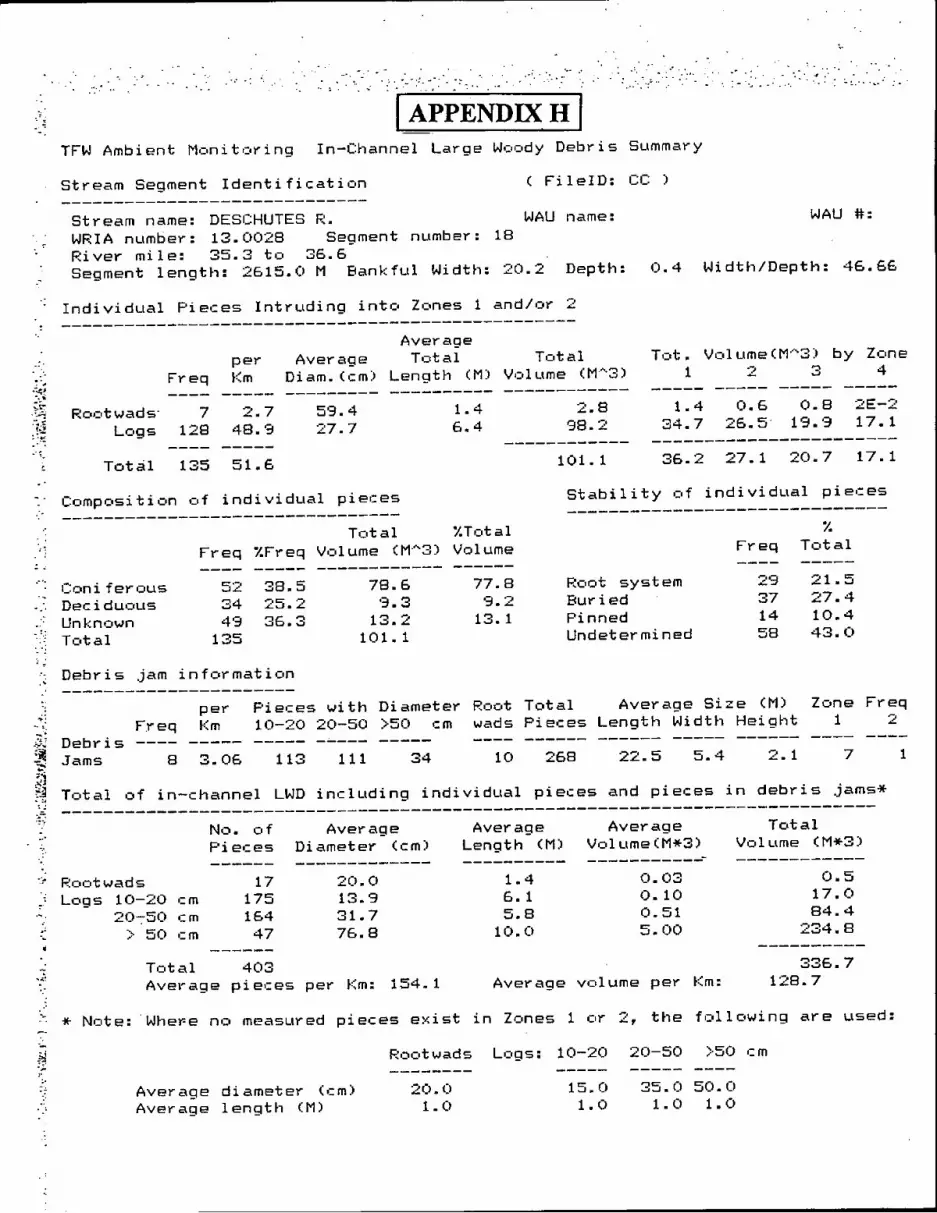
I~PPENDIX H I TFW Ambient Monitoring In-Channel Large Woody Debris Summary

Stream Segment Identification ( Fi leID: CC ) -----------------------------

Stream name: DESCHUTES R. WAU name: WAU #:

WRIA number: 13.0028 Segment number: 18 River mile: 35.3 to 36.6 Segment length: 2615.0 M Bankful Width: 20.2 Depth: 0.4 Width/Depth: 46.66

Individual Pieces Intruding into Zones 1 and/or 2 -------------------------------------------------

per Km

Average Average Total Total Tot. VolumeCM A 3) by Zone

-'.-

Freq Diam.(cm) Length (M) Volume (M A 3) 1 2 3 4

7 128

2.7 48.9

59.4 27.7

1.4 6.4

2.8 98.2

----- ----- ----- -----1.4 0.6 0.8 2E-2

34.7 26.5· 19.9 17.1 ROI:rtwads'

Logs ------------ -----------------------

Total 13551.6

Composition of individual pieces --------------------------------

Coni feyous Deciduous Unknown Total

Total %Total Freq %Freq Volume (M A 3) Volume

----- ------------ ------52 38.5 34 25.2 49 36.3

135

78.6 '3.3

13.2 101. 1

77.8 9.2

13.1

101. 1 36.2 27.1 20.7 17.1

Stability of individual pieces ------------------------------

Root system Buried Pinned Undetermined

% Freq Total

2'3 37 14 58

21.5 27.4 10.4 43.0

.~ Debris jam information

per Km

Pieces with Diameter Root Total Average Size (M) Zone Freq

"'. _. F.req 10-20 20-50 )50 cm wads Pieces Length Width Height 1 2

iii Debr i s ; Jams 8 3.06 113 111 34 10 268 22.5 5.4 2.1 7

ti i ~~

Total of in-channel LWD including individual pieces and pieces in debris jams* -----------------------------------------------------------------------------

No. of Average Pieces Diameter (cm)

Average Length (M)

Average Volume(M*3) ------------

Total Volume (M*3)

·c- Rootwads Logs 10-20 r:m

em em

17 175 164 47

20.0 13.9 31.7 76.8

1.4 6. 1 5.8

0.03 0.10 0 .. 51 5.00

0.5 17.0 84.4

234.8 20-:-50

> 50

Total 403 Average pieces per Km: 154.1

10.0

Average volume per .(m: 336.7

128 .. 7

* Note: ·Whe~e no measured pieces exist in Zones 1 or 2, the following are used:

Average diameter (em) Average length 1M)

Rootwads Logs: 10-20 20-50 )50 em

20.0 1.0

15.0 1.0

35.0 50 .. 0 1.0 1.0

1

Timber-Fish-WiIdlife Ambjent Monitoring Program

SALMONID SPAWNING GRAVEL COMPOSITION

MODULE

August 1994

Dave Schuett-Hames Bob Conrad

Mike McHenry Phil Peterson Allen Pleus


SALMONID SPAWNING GRAVEL COMPOSITION MODULE

Contents


Introduction ..... , ............................................................................................................ 3

Purpose of the Spawning Gravel Composition Module ............................................... 4

The Spawning Gravel Sampling Methodology ............................................................ 4

Information and Equipment Needed ................ .... ... ... ... ...... ..... ... ... ....... ... ..... ..... ....... ..... ......... 4 Site Selection ............. '" ... ... ..... ... ... ......... ....... .......... .............. ... ..... ..... ... ..... ..... ....... ....... ........ 5 Determining a Sampling Method ........................................................................................... 8 Inventory of Sampling Reaches ............................................................................................ 10 Sample Population: Systematic Random Sampling Strategy ... ..... ... ..... ..... ..... ..... ....... ....... ... 13 Collection of Samples ....................................................................................................... ·... 14

Methods for Processing Spawning Gravel Samples .................................................. 2I

The Volumetric Processing Method .......................................................................... 2 I

Equipment Needed ................................................................................................................... 21 Processing Samples ..................................................................................................................... 22

The Gravimetric Processing Method ......................................................................... 28

Equipment Needed.. ......... .... ........ ... ... ............. ................. ... ..... ...... ..... ..... .... ...... .... ....... ...... .... 28 Processing Samples.................................................................................................................. 29

Data Analysis ........................................................................................................... 29

Data Analysis for Individual Samples....... .................... ...... ... ........ .......... .... .... ....... ..... ....... ... 30 Data Analysis for Stream Segments........ ... ... ... ....... ... ..... ... ... ... ..... ... ..... ..... ..... ..... ..... ..... ........ 30

Training, Field Assistance and Quality Control... ...................................................... 3 I

References ................................................................................................................ 31

Appendixes.............................................................................................................. 35

1994 TFW Ambient Monitoring Manual Spawning Gravel - I

Acknowledgements

Thanks to Jeff Cederholm, Jim Matthews, Doug MOTTel, Mark Teske, George Pess, and Martin Fox for providing data and assistance in the development of the salmonid spawning gravel module.

Cover: Dave Schuett-Hames on Thurston Cr. Photo by Allen Pleus. Module illustrations and photographs by Allen Pleus unless noted.

1994 TFW Ambient Monitoring Manual Spawning Gravel - 2

SALMONID SPAWNING GRAVEL COMPOSITION MODULE

Introduction

. The development of salrnonid eggs and alevin typically occurs in the gravel substrate of freshwater rivers and streams. Mature females choose sites where·substrate and flow conditions are favorable and deposit their eggs in nests (redds) they excavate in the substrate. After the eggs hatch, the a1evins continue to reside within the streambed gravel, subsisting on nutrients from an external yolksac. When the yolk-sac has been absorbed they emerge from the gravel and begin active feeding.

The eggs and alevin require a stable streambed and an adequate supply of water while developing to prevent dehydration, supply oxygen and carry away metabolic waste. Mortality during intra-gravel development is highly variable, depending on hydrologic, geomorphic and biotic conditions. MortalitY has been attributed to a variety of causes including disease, predation, suffocation, dehydration, mechanical disturbance and freezing (McNeil, 1969).

How Fine Sediments Affect the Incubation Eiwironmerit

Salrnonid eggs require an abundant supply of dissolved oxygen to ensure survival to emergence and proper development (Alderdice et aI., 1958). Oxygen reaches the eggs through a three-step process involving dissolution of oxygen from the atmosphere ·into stream water, transport of oxygenated water to the stream bottom, and interchange of oxygenated water from the stream to the pores between gravel in the egg pocket (Vaux, 1962). Fine'sediment (fine sand, silt or clay) that lodges in the interstitial spaces between gravel particles reduces permeability and slows the rate of flow through the gravel substrate (McNeil and Ahnell, 1964; Johnson, 1980). Numerous studies (Chapman, 1988, Everest et a1., 1987; Iwamoto et al. 1978) have associated high levels of fine sediments with elevated mortality rates and reduced fitness of surviving fish (Koski, 1975). These effects are due to increased stress and mortality associated with oxygen deprivation (Alderdice et a1., 1958), the accumulation of toxic metabolic by-products(Bams and Lam, 1983), and entombment of emerging fry (Chapman, 1988).

Natural and Management-Related Sources of Fine Sediments

Concentrations of fine sediments in stream channels vary in space and time (Adams and Beschta, 1980). The amount of fine sediments present at a particular location depends on the nature and magnitude of erosional processes that produce fine sediments and introduce them to the stream channel, as well as the geomorphic factors that control the transport and storage of sediments, such as stream gradient and. hydrology. In addition, spawning salmonids tend to remove fine sediments from the substrate during redd construction; howevertlie persistence of this effect is not well understood (Everest et al. 1987). During the incubation period, fine sediments moving through the stream channel may intrude into the redd. The severity and significance of fine sediment intrusion is

1994 TFW Ambient Monitoring Manual Spawning Gravel· 3

related to the size and amounts of transported sediment, and the depth of intrusion (Lisle, 1989). Fine sediment levels are higher in watersheds where the geology, soils, precipitation or topography create conditions favorable for erosional processes that produce fine sediments (Duncan and Ward, 1985). Fine sediments are typicaUy more abundant where land-use activities such as road-building or land-clearing expose soil to erosion and increase mass wasting (Cederholm et aI., 1981; Swanson et aI., 1987; Hicks et aI., 1991).

Purpose of the Spawning Gravel Composition Module

The purpose of this module is to provide a standard method of sampling potential salmonid spawning habitat to characterize gravel composition and fine sediment levels on a stream segment scale in streams where there is no prior data available on variation in gravel composition to guide sample design. (For streams with existing data, it may be preferable to develop custom sampling strategies based on segment-specific variation). The intent is to ensure replicable data that aUows comparisons to be made through time and between stream segments. The information generated on the condition of potential spawning habitat is suitable for use as a management indicator. The module does not attempt to document or predict actual survival to emergence, because that objective would require research of an intensity impractical for management purposes. Nor is it oriented towards the requirements of any particular salmonid species, as species may vary within and between stream segments around the state.

The information generated using this methodology is suitable for:

* evaluating the composition and characteristics of spawning gravel; * estimating the percentage of fine sediments less than 0.85 mm for Watershed Analysis; * comparing spawning gravel composition among stream segments, watersheds and eco-regions; * monitoring trends in spawning gravel composition over time.

The Spawning Gravel Sampling Methodology

This section will cover what information and equipment is needed, site selection, determining a sampling strategy, inventory of sampling sites, and coUectil/n of samples from the stream.


Map delineating stream segments *McNeil sampler with plunger *Fiberglass tape (30, 50 or 100 meter, depending upon channel width) Plastic buckets (5 gallon) with lids- one per sample Backpack carrier for buckets (optional) Squirt bottles (2) Hip boots or chest waders Rain gear (* Calibration required)


Form 6.0 Form 6.1 Field notebook Pencils Permanent markers Flagging Bucket labels

Spawning Gravel - 4

Field Note: (1) The plastic buckets and lids should be sequentially numbered with a permanent marker prior to taking them out in the field. (2) The equipment needed for processing samples depends upon the method used. The equipment requirements of each processing method are discussed separately in the sections on ''volumetric processing" and "gravimetric processing".

Calibration

Check the McNeil sampler for damage. There should be no broken welds, holes, or dents sufficient to cause changes in volume of sample taken. Measure the coring cylinder length from the top of the stop ring to the base of the collection basin. The standard length should be 23 cm. Next, measure the inside diameter of the coring cylinder. The standard diameter should be 15 cm. If your coring cylinder has different dimensions, make a note of it. Check the plunger for damage. Tighten any loose fittings and replace defective washer/seals and flap valves.

Calibrate your fiberglass tapes using the methods outlined in the Reference Point Survey Module calibration section. Record all information in your QA plan.

Site Selection

Prior to inventorying sampling sites and collecting samples, it is necessary to determine which segments are best suited to gravel sampling and then identifying the logistically feasible sampling reaches within it.

ApPTQpriate Times to Collect Samples

Spawning gravel composition (particularly fine sediment levels) in a stream reach can vary over the course of the year. In western Oregon streams, substrate composition was relatively stable from early summer to early fall, and was most variable during the winter storm season when peak flows mobilized the substrate and the processes of fine sediment infiltration were most active (Adams and Beschta, 1980). In order to provide a management indicator of substrate composition that can be used to compare stream reaches and determine trends over time, sampling should be conducted during moderate to low flow conditions outside of the winter-spring high runoff period. The actual timing of the high runoff period will vary depending on the hydrologic regime of the system. If you are unfamiliar with the system to be sampled, consult with people familiar with the system or refer to USGS stream flow records to determine an appropriate sampling period.

Collecting spawning gravel samples during extremely low flow conditions is also to be avoided, because only a small portion of the potentially available spawning habitat will be wetted. This may introduce bias into site selection. We do not recommend sampling areas that do not have water flowing over them such as dry, exposed bars because the potential effect this may have on the sampling process or the composition of the sample is unknown.

It is usually ideal to sample in the late summer/early fall low flow period when conditions are similar to those encountered by salmonids when they begin to spawn. Avoid working in the channel


during spawning or when there are eggs in the gravel, to prevent unnecessary disturbance and mortality to salmonid populations.

IdentitYjng Sampling Segments

Delineation of stream segments is the first step in selecting a sampling reach. This methodology characterizes spawning gravel composition at the stream segment scale. Stream segments, reaches distinguished from one another by changes in gradient, valley confinement or tributary confluences, are the fundamental unit of analysis. This step may already have been done during Watershed Analysis or previous Ambient Monitoring surveys. If so, use the segment maps generated and skip this step. If not, partition the river system into stream segments using the TFW Ambient Monitoring Stream Segment Identification Module.

Ilk"6lllcl:ll9 I - -- --- --------- ......, .... _""-- -- -- -- -- - ---------

oat.1 ~ 1% 1 > oat.2 ~ 2%

2> oat.a < 4% 4> oat.4 ~ 6%

Best

6 > oat.4 < 8% lhsUtt:tlIe 8 > oat.S :< 20% 20% > oat.6-

ILlSOblii I

ll.t<tlle I

----------------------------~~~

Figure l. Suitability of gravel sampling by segment and gradient.

1994 TFW Ambient Mouitoring Manual

Choosing Appropriate Segments to Sample

Once the river system has been divided into segments, the criteria used to select appropriate monitoring segments should include salmonid use (current, historic, or future potential), appropriate gradient, and substrate size. The McNeil sampler does not work well in substrates with particles greater than ten cm (four inches) in diameter.

-"This methodology is best suited for segments consisting of pool-riffle sequences (typically gradients less than two percent). It can sometimes be applied (with modifications) on segments in the two-to-six percent range where spawning gravels typically occur in patches, but is usually unsuitable for segments with gradients over six percent (Figure 1). For segments with a category 4 gradient (4 - S%), it is necessary to know the average map gradient based on USGS 7.5 minute topographic maps in order to select those segments with 4 - 6% gradient.

Logistically Feasible Sampling Areas

Once a segment has been chosen for sampling, the next step is to identify portions of the segment suitable for sampling and to eliminate portions where sampling is logistically irn-

Spawning Gravel - 6

practical. Ideally, sampling sites should be distributed throughout the entire segment. However, this is not always practical due to the size and weight of the sampler and the gravel samples, proximity to vehicle access, and stream channel features. Alternative transport systems such as helicopters or boats may provide better access.

Examine the segment and identifY potential access roads and trails, and terrain features that impede access. Then determine how far it is feasible to transport equipment and samples to the access points. This will depend on the terrain and the physical strength and endurance of those transporting the samples. Transporting samples for distances greater than 0.75 - 1.0 kilometer is probably not practical in most cases (Figure 2).

Eliminating Areas in the Vicinity oOnstream Structures

Human structures and disturbance in the stream channel such as bridges, culverts, weirs, dams, bank protection, fords, etc., locally alter hydraulic conditions in stream channels, affecting sediment deposition patterns. Samples taken in the vicinity of these structures or disturbances reflect the local effects of the structure and mask the overall effect of watershed conditions on the stream channel. Avoid sampling within the immediate influ-

~ ... z: o .... ~ IoU .... .... = ID

no aceelJ

Bridge

WDF Weir -+:;::>';;'4.).)" -Private Farm -

Alk permlulon to crOll or get .hot It

Cow ford

Bridge

~~~~~~~~.~ .. ~

o

Main aCClII road

Figure 2. Detennining and finalizing potential sampling areas in segment reaches 1 and 2 based on topographic map and local knowledge. The circular areas are the finalized areas for sampling.

ence of these features. The length of affected stream channel will vary, however as a general guideline do not collect samples within 50 meters of instream structures.

Finalizing the Sampling Reach

Once areas that are logistically impractical to sample or are in the immediate vicinity of instream structures have been eliminated, the remainder of the segment is available for sampling and is referred to as the sampling reach.

1994 TFW Ambient Monitoring Manual Spawning Gravel -7

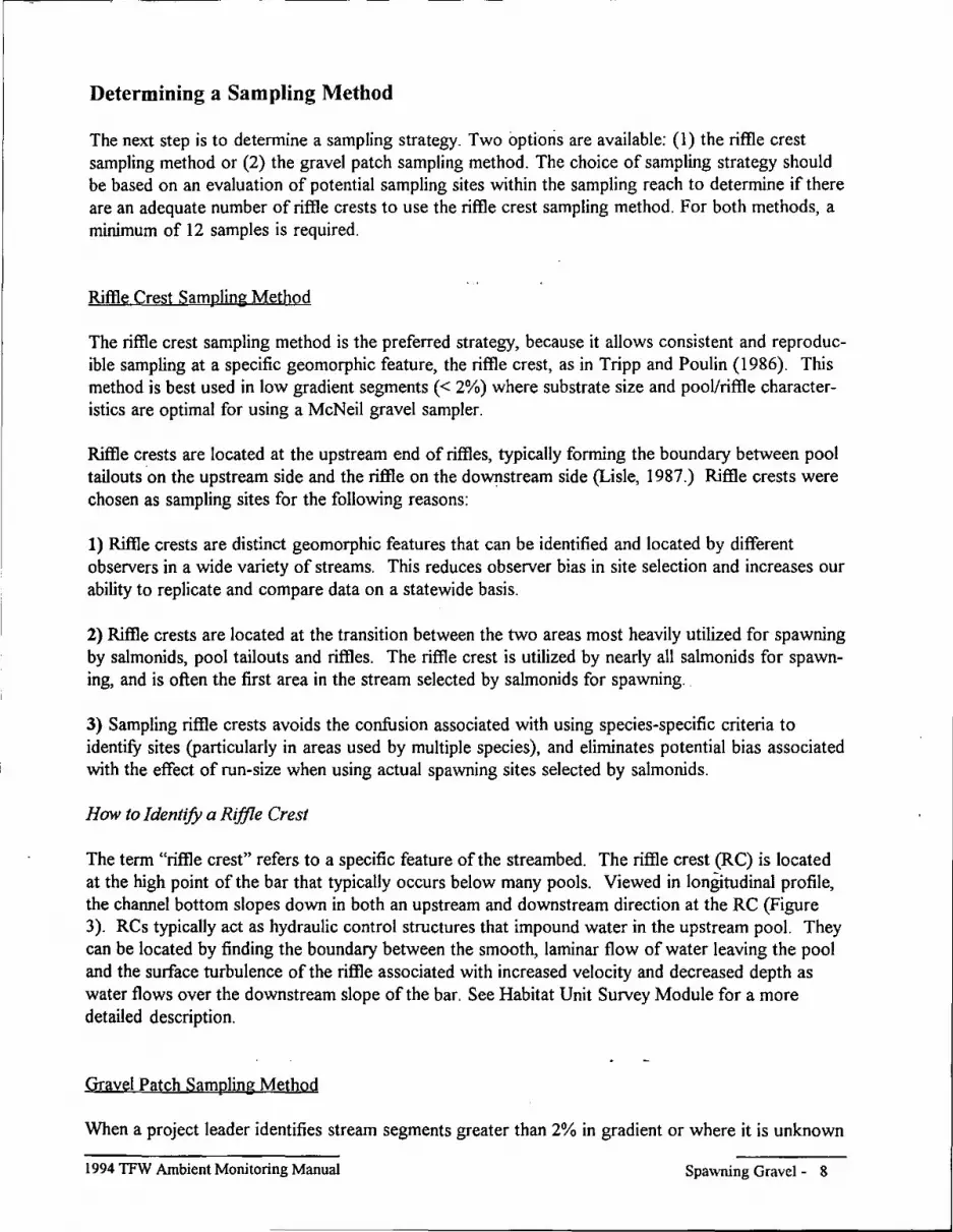
Determining a Sampling Method

The next step is to determine a sampling strategy. Two options are available: (1) the riffle crest sampling method or (2) the gravel patch sampling method. The choice of sampling strategy should be based on an evaluation of potential sampling sites within the sampling reach to determine if there are an adequate number of riffle crests to use the riffle crest sampling method. For both methods, a minimum of 12 samples is required.

Riffle Crest Sampling Method

The riffle crest sampling method is the preferred strategy, because it allows consistent and reproducible sampling at a specific geomorphic feature, the riffle crest, as in Tripp and Poulin (1986). This method is best used in low gradient segments « 2%) where substrate size and pool/riffle characteristics are optimal for using a McNeil gravel sampler.

Riffle crests are located at the upstream end of riffles, typically forming the boundary between pool tailoutson the upstream side and the riffle on the downstream side (Lisle, 1987.) Riffle crests were chosen as sampling sites for the following reasons:

1) Riffle crests are distinct geomorphic features that can be identified and located by different observers in a wide variety of streams. This reduces observer bias in site selection and increases our ability to replicate and compare data on a statewide basis.

2) Riffle crests are located at the transition between the two areas most heavily utilized for spawning by salmonids, pool tailouts and riffles. The riffle crest is utilized by nearly all salmonids for spawning, and is often the first area in the stream selected by salmonids for spawning.

3) Sampling riffle crests avoids the confusion associated with using species-specific criteria to identifY sites (particularly in areas used by multiple species), and eliminates potential bias associated with the effect of run-size when using actual spawning sites selected by salmonids.

How to Identify a Riffle Crest

The term "riffle crest" refers to a specific feature of the streambed. The riffle crest (RC) is located at the high point of the bar that typically occurs below many pools. Viewed in longitudinal profile, the channel bottom slopes down in both an upstream and downstream direction at the RC (Figure 3). RCs typically act as hydraulic control structures that impound water in the upstream pool. They can be located by finding the boundary between the smooth, laminar flow of water leaving the pool and the surface turbulence of the riffle associated with increased velocity and decreased depth as water flows over the downstream slope of the bar. See Habitat Unit Survey Module for a more detailed description.

Gravel Patch Sampling Method

When a project leader identifies stream segments greater than 2% in gradient or where it is unknown


Pool

I

Riffle

I

I Riffle I Crest #1 I

SuboIroto ........ _-

I

I

I I

Pool

I Riffle I Crest :fI!2

Figure 3. Plan and profile views of a stream reach identifYing the location of riffle crests.

I PLAN VIEW I

I !'RORLE VIEW I·

if there are enough RCs to produce 12 samples, it is recommended that you inventory both RCs and patches to determine which method to use. The gravel patch method is recommended when there are not enough riffle crests or when the riffle crests are too heavily armored with large particles to collect an adequate number of samples with the McNeil sampler. This method is useful in steeper streams where the pool-riffle sequences typically are less well defined and the riffle crests contain larger particles. In these situations, spawning gravels typically occur in patches associated with obstructions or the tail outs of large pools. The patch method has a minimum guideline of 12 samples per segment.

Haw to Identify a Gravel Patch

The definition of a gravel patch covers a broad range of potential spawning gravel situations. Basically, a patch is one contiguous formation of suitable spawning gravel covered by water under summer low-flow conditions. The guideline for the minimum size of a patch is two square meters, but this may vary depending upon local conditions or redd size characteristics required of the species which utilizes (or potentially utilizes) that segment of stream. The minimum size is also a consideration of equipment limitations in regards to the potential for a successful sample collection. Patches are most often located on the downstream side of an obstruction such as a log or boulder, in the tailout of a pool, along the submerged edge of a gravel point bar, and sometimes as a portion of a riffle unit. Riffle crests are treated as patches when there are too few to meet the minimum number necessary to use the riffle crest sampling method.

1994 TFW Ambient MonitOring Manual Spawning Gravel - 9

Inventory of Sampling Reaches

At this point, you should have completed your segmenting and defined your sampling reaches within the segment. For this section, you will need a map of the stream segment showing reaches, access points or local conditions to be aware of, several blank copies of Form 6.0 (Appendix A), flagging and permanent markers, hipboots and other appropriate field gear.

The first task is to determine which sampling method to employ. To do this, use the suitability index (Figure 1) as a guideline. If the segment gradient is less than 2%, a systematic riffle crest inventory strategy is generally the most suitable and usually only riffle crests would be inventoried. If the segment is greater than 2%, then both riffle crests and patches are inventoried unless local knowledge indicates that there are enough suitable riffle crests.

Once the sampling method is decided, the next step is to inventory the segment's sampling reaches to . determine the total sampling population using Form 6.0. For the riffle crest method, walk the entire

length of each sampling reach and inventory all riffle crests (RCs) with 2 or 3 estimated sampling sites. For the patch method, walk the entire length of each sampling reach and inventory all riffle crests and patches with 1, 2, or 3 estimated samples.

The evaluation of a sampling site to estimate the number of potential samples is based on several factors. First, determine the spawning gravel area in regards to substrate size and obstructions. Second, estimate the number of samples possible considering the diameter of the equipment, the area of equipment disturbance created by attempting a core, and the area of human disturbance caused when trying to provide stable footing. As a guideline, samples should be taken a minimum of 1 meter apart. Third, record the number of undisturbed samples physically possible (minimum-II maximum-3 per site). Be sure to eliminate sites that have been disturbed by human activities as described above.

During the inventory, riffle crest and/or patch sites that appear suitable for sampling (1-3 potential samples) are assigned unique riffle crest (RC #) or patch (P #) numbers. Begin at the downstream end of the segment and assign the RC and P numbers sequentially by type throughout the sampling reaches. Using Form 6.0, record the number assigned to each suitable RC or P and note its location relative to a reference point or landmark. Marking the location on aerial photographs provides another level of documentation. In the stream, mark each suitable RC or P site with flagging showing the RC or P number. The complete set of suitable riffle crest and/or patch sites identified within the segment's sampling reaches constitutes the pool of potential sampling sites from which the systematic inventory strategy is applied to determine a final sampling population.

Systematic Riffle Crest Inventory Strategy

In low gradient stream segments where you have high confidence that there are enough riffle crests to provide a minimum of 12 samples, inventory only riffle crests with 2 or 3 estimated samples. For example, Figure 4 shows the inventory strategy for riffle crests using Form 6.0. The riffle crests are numbered sequentially (RC #), the estimated number of undisturbed samples possible from the RC are noted, and the sampling site location is established by assigning distances from the nearest reference point (RP #) or other landmarks as necessary.


I SPAWNING GRAVEL COMPOSITION I i~;~~FUl1i:~ roquu.d on fu>l form for . I each day ~initials can be I W.R.LA. Lt. 0 01..1::.-_. ___ L ~ ~ socondary P!!." .J INVENTORY

Segment # b 0 L8 ORB Stream Name i(.fiNN 1::1'> Y (jlG:E:1<.

Basin Name Sf/CLTON Inventory Date .!LIJ£I 1t./ Rivermile from ':t..o to 'I,S- :f,scgment 0 ~ _!LJ£I Ci'f. g Gradient ~ Yo to Ref. Pt. from IS) to

Inventol}' Lead 6l.<-1..i;w p(£<.<S Affiliatioo N <,) I.f-C.-

Recorder O!!l.vt: ~l..r:f.'( Err -1I",m<:~ 61 "" f::f

RifIIc Cn:sI Paid> Samples Landmark Up

SP# RC# P# Est. # RP# Distance I ;, Field Notes

I 1\ (s) ~ ~o ,.., : UP Coco sIre - NO ~fr .. cf,'b~s

2 \ / z. IQ 70 ..... I I.\f I Lur~ e (p 1 I,f:;;./'.'..~ Y3 /I.e ON L8

:3 \ / (J) I ;-If'1 I lAp Gooo sITe I.( \ / ~ I 3r-/VI i Sff'/IILI..II.C. "" ),~"Y fool Un:/-

~ \ / 2- I ~O ""l I l If tt.6{; Co84I.E I'R E:SE; "'r h I

Z- Z. §),., : 10 " .. 7 (:J 3 2.~ ..... I i bOOt> 5!T1= - A~~;~ u e~v ~ j \ (j) 10 60/VI ! (JOOO 51T~

tj / _\ 2- 7 /),.., i Ih .. " '1CS fl.1]

to / \ 2- 7 '?o,.., I • INT~" IJ~ /l./J f /...8

11 II \ 2- 7 hO /(l : t./ltt(,~ (P(J8~ I'{ 8

Il- I (j) I? ,,5:1"1 I ,,. I &co() $ITE _ C4~T/f>J! ::~;'T L8

! I

Figure 4. Form 6.0 showing the riffle crest inventol}' strategy

After inventorying the sampling reaches of your segment on Form 6.0, count the number of estimated samples for all RCs.

a.) If the total estimated number of samples falls between 12-18, the result constitutes your total sampling population from which 100% of the RCs must be sampled for the segment. Skip the rest of this section and go to the "IdentifYing Sampling Points at Rifile Crest and Patch Sites" section (pg. 15). b.) If the number is greater than 18, the result constitutes your sampling population from which a random sub-sample is taken (Figure 5). Skip the rest of this section and go to the "Sample Population: Systematic Random Sampling Strategy" section (pg.13). c.) If the total estimated number of samples is below 12, you will need to re-inventory the segment using the systematic patch inventory strategy below.

19941FW Ambient MonitOring Manual

Riffle Crest Method

RC # N RC Samples

w/3 f" " --

w/2 7 ~

Figure 5. Number ofRCs and Samples.

Spawning Gravel - II

Systematic Patch Inventory Strategy

This strategy is useful in higher gradient stream segment situations (>2%) where you do not know if there are enough riflle crests to provide the minimum 12 samples. In this strategy, walk the stream starting from the downstream end and identityfmventory all riffle crests and patches sequentially on Form 6.0 (Figure 6). At the end of the segment, assess the number of samples possible from using only RCs with 2 or 3 estimated samples. If the estimated sample number is greater than 12, (and this

RifIlc Crest PaU:b Samples . SP# RC# P# Est. #

/ , J J 2-

'- 2- 2.

3 2- (3) /' I

Lj J 2

X I

S I..{ -z.. Co >" 2-

;6 I

7 S 2-

8 7 2-

% I q 2r 2-

10 G) (3)

FIgure 6. Detail of Form 6.0 shOWIng the systematic patch inventory strategy

b.) If the number is greater than 18, the result constitutes you( sampling popula-tion from which a random sub-sample is taken. Eliminate all sampling sites with only 1 estimated sample and adjust your sampling population number (SP #) on Form 6.0 to reflect the proper sequence (Figure 7). Skip the rest of this section and go to the "Sample Population: Systematic Random Sampling Strategy section" (pg.13).

1994 1FW Ambient Monitoring Manual

characterizes the segment for your purposes) use the systematic riffle crest inventory strategy outlined above and eliminate all patches and riflle crests with only 1 estimated sample. If the number is less than 12, lump the riffle crests and patches together into the systematic patch inventory strategy.

The systematic patch inventory strategy foUows the same format as the riflle crest inventory strategy except that both riflle crests and patches are now part of the same total sample population. After mventorying the sampling reaches of your segment on Form 6.0, count the number of estimated samples for aU riflle crests and patches with 2 or 3 estimated samples.

a.) If the total estimated number of samples faUs between 12-18, the result constitutes your total sampling population from which 100% of the RC/Ps must be sampled for the segment. Eliminate aU sampling sites with only 1 estimated sample and adjust your sampling population number (SP #) on Form 6.0 to reflect the proper sequence. Skip the rest of this section and go to the "IdentifYing Sampling Points at Riffle Crest and Patch Sites" section (pg. IS).

RC # # Patch Method RC Samples

w/3 R- ~ w/2 3

; \ RCIP R~ #

wll ..L Samples

-- w/3 ~ fo

p # # V w/2 l? ~ p Samples --

wll 2.... S-w/3 -z. 0 w/2 ~ ~ w/l ~ ~

Figure 7. Patch method: enumeration of rifile crests and patches - lumping into combined sampling sites (RC/P).

Spawning Gravel - 12

c.} If the total estimated number of samples is below 12, include all riffle crest and patch sites with I estimated sample. Repeat the strategy listed above, but ignore the section on elimination.

Note: There may be times when a complete inventory of a segment produces a sample population with less than the guideline of 12 estimated samples. A low sample population could be the result of many factors such as stream and segment size, substrate armoring, or access. Ultimately, it is up to the cooperator to determine whether such a low sample population adequately characterizes their segment.

Sample Population: Systematic Random Sampling Strategy

At this point, you should have a completed Form 6.0 from which identifies your sampling population. The following systematic sampling strategy was developed by examining four existing large data sets from Washington State to determine variation within and among riffles. It uses a two-stage sample design with riffle crests as the primary sample units and samples within riffle crests as the secondary sample units. Systematic sampling of riffle crests (with a random starting point) is recommended to avoid potential clustering, because fine sediment may systematically increase in a downstream direction if gradient decreases. Based on the existing data we examined, a coefficient of variation of less than 20% can be achieved by collecting a minimum of three samples per riffle crest and sampling as many riffle crests as possible, but no fewer than 10% of the total riffle crests in each segment. The following recommendations for sampling are based on the number of riffle crest and/or patch sites inventoried in the stream segment. The objective is to maximize the distribution of sampling sites, but within the logistical constraint of keeping the total number of samples per segment under 20.

To determine the number of riffle crest and/or patch sites to sample, refer to your inventory Form 6.0. In the left hand column of Table 1, locate the appropriate row corresponding with the segment riffle crest and/or patch inventory total. The second column on that row will state the percentage of sites to be sampled. For example, if 17 riffle crests were inventoried, then the third row (13 - 18) would be selected so 33% of the riffle crests should be sampled.

Table I. Recommendations for sampling riffle crest (RC) and patch (P) sites.

-Total No. Pe rcent of sites Choose random Total

RCs andPs sampled number between Samples

4-6 100% - 12 -18 7 - 12 50% 1-2 12 -18

13 - 18 33% 1-3 12 -18 19 - 24 25% 1-4 12 - 18 25 - 30 20% 1-5 12 -18

> 30 12.5% 1-8 12+


Next, select a random starting number using a random number generator, die, or a random number table (provided in Appendix B). Use the third column in Table I to determine the appropriate range of random numbers to select from. Then find the appropriate box in Table 2 to detennine the sequence of riffle crests and/or patches to sample. Circle the corresponding numbers in the SP # column of Form 6.0 to identifY those which will be sampled in the field.

SfT" (fl,</p) Table 2. Selection of systematic sampling.sequences.

Random 50% 33% No. . .

1 1,3,5,7 9,11 1.4,7,10,13,16

2 2,4,6, B,10, 12 2,5,8,11,14,17

3 3,6,9,12,15,18

• 5

• 7

• ..

Selecting Additional Random Sampling sites

25% 20% 12.5%

1,5,9,13,17.21 1,6,11.16,21,26 1.9,17,25,33, 41 etc.

2,6,10.14,18,22 2,7,12,17,22,27 2,10, IS·, 26, 34, 42 etc.

3,7,11,15,19,23 3,8,13,18,23,28 3,11,19,27,35, 43 etc.

4,8,12,16,20,24 4,9,14,19,24,29 4,12,20,28,36, 44 etc.

5,10,15,20,25,30 5,13,21.29,37, 45 etc.

6,14,22.30,38, 46 etc.

7,15,23,31,39, 47 etc.

8,16,24,32,40; 48 etc .

There may be instances where the random sequence does not provide enough sites to collect 12 samples. In these cases, randomly select additional sampling sites as needed from the un selected sample population and circle the SP # on Form 6.0.

Collection of Samples

At this point, the cooperator should be ready to collect actual gravel samples. For this section, you will need your completed Form 6.0, several blank copies of Form 6.1 (Appendix C), and all field equipment outlined in the "Information and Equipment Needed" section.

Start by locating on the stream your first sampling site as listed on Form 6.0 (SP #\). The next step is to determine the specific points on the rifile crest or patch to sample. The most important part to remember is that this method is for an analysis of salmonid spawning gravel. This means that any given length of riffle crest or size of patch may not constitute \ 00% gravel suitable for spawning. There are three common characteristics of spawning gravel used to determine the dimensions of the spawning gravel section of a rifile crest or patch: (1) must be covered by flowing water - gravel under eddies or stagnant water are not included; (2) avoid depositional areas where sand/silt are dominant - usually along wetted edges; and (3) factors limiting the use of the sampling equipment -the gravel composition is dominated by substrate more than \ 0 cm diameter, gravel under/near logs, boulders, or jams.

1994 TFW Ambient Monitoring Manual Spawning Gravel· 14

Jdenti&ring Sampling Points in Riffle Crest and Patch Sites

At each riffle crest selected for sampling, samples are taken on a line extending across the spawning gravel section along the top of the riffle crest. If the riffle crest extends diagonally across the channel, the line should follow the riffle crest.

Begin by extending a fiberglass tape across the wetted portion of the spawning gravel of the riffle crest. Three samples should be taken at each riffle crest site. The first sampling point is the midpoint of the line across the spawning gravel of the riffle< crest. Place a marker (flagged weight) at this point. Next, measure two-thirds ofthe way' between the mid-point of the cross-section and the wetted gravel perimeter towards the left bank and mark this location. Last, measure two-thirds of the way from the mid-point to the wetted gravel perimeter towards the right bank and mark this location. If the spot selected is on a small dry bar, too close to a log or boulder, or in still water, go to the nearest suitable location along the line. If a sampling point is lightly covered with organic debris such as leaves or twigs, gently remove them without disturbing the gravel underneath. The resulting three markers are the sampling points for the riffle crest (Figure 8).

On many stream systems, it is necessary to make several coring attempts with the McNeil gravel sampler before a successful sample is taken. This commonly occurs when the buried substrate is too large for the coring cylinder. If you are unsuccessful taking a sample at a selected location because of this or other reasons, try sampling laterally along the transect, remaining as close to the original point as possible but beyond any gravel disturbance caused by the cylinder or footholds. In situations where you are unsuccessful in collecting any

x = samplIng points on riffle crest

Scmp/Irg sHes 1d<en at m\q:>olnt of spay.nlng I1avElI on riffle crest en:! at 2fJ back1o\.t.crds

LB en:! RB edge of spay.nlng gavel.

Figure 8. Sampling points at rifile crests.

samples from a riffle crest, randomly select either the upstream or downstream adjacent riffle crest (flip a coin) and collect the samples at this location. Be sure to note this change on your Form 6.0 or in your field notebook.

1994 TFW Ambient MonitOring Manual Spawning Grnvel -15

RC~# 3 Samp e# b Bucket # ~I

Notes: £5~~ ",.kj t.'2.u..k~ i" xeJl;:: f" ,.,{ /)12.0 l. rcl~Q-1,l~

~lii~'" a 8.1> ,£/1<. ...

'-FIgure 9. Detail of Form 6.1: Example of coUection information.

When a successful sample has been taken, use Fonn 6.1 to document all pertinent collection infonnation. For each sample, note its RC # or P # (circle appropriate type), the Sample #, the Bucket #, plus any notes such as local conditions and number of attempts before successful (Figure 9).

At each patch selected for sampling, the shape of the patch helps to determine the pattern used to take gravel samples. If the patch shape is linear, follow the guidelines above for identifying sampling points in riffle crests. If the patch shape is large and wide enough, then use a triangular pattern to identifY sampling points.

Collecting Samples with the McNeil Grayel Sampler

The McNeil sampler was selected to collect samples of spawning gravel for analysis as recommended by Peterson et al. (1992). It was chosen for the following reasons:

1) it is a reliable sampling device that is simple to operate;

2) although bulky, it is relatively portable and requires little auxiliary equipment;

3) it has been used in Washington State for survival to emergence studies that were the basis of the Forest Practices Board cumulative effects threshold values for spawning gravel fine sediments.

The McNeil gravel sampler is designed to take a core sample ofthe gravel substrate. A schematic diagram of the sampler is shown in Figure 10. The bottom of the sampler consists ofa 15 cm (6 inch) diameter stainless steel coring cylinder with an open bottom and top. The coring cylinder is designed to penetrate into the streambed gravel to a depth of23 em (10 inches). The top of the coring cylinder extends up through the bottom of the larger (35 cm diameter) collection basin, where gravel from the core is temporarily stored during excavation of the core. The collection basin is open on the top. A horizontal steel rod attached across the top of the collection basin acts as a handle.

There is also a plunger, inserted into the coring eylinderiCi'retain sediment-bearing water after extraction of the sample. The plunger consists of two metal disks, just slightly smaller in diameter than the inside of the coring cylinder, attached to the end of a long handle. Between the metal disks is a piece of neoprene that is slightly larger than the inside of the coring cylinder and acts as a seal. A hole through the disks with a one-way flapper valve allows the plunger to be inserted without forcing the water down into the streambed, but prevents water from escaping when the sampler is lifted. When fully inserted, the plunger comes to rest on a small stop-ring on the inside of the coring cylinder.

19941FW Ambient Monitoring Manual Spawning Gravel - 16

Coring handle 1---------,

I Koski

Plunger I

COlleCtion! Cylinder I

===n==:::J Handle

Carrying handle

Stainless Steel Cylinders

McNeil Cylinder (Modified) I

r_-;:::=1=::::;--;:;-r'i-=colleCtion II . basin I

I I I I One-way

Top view

Suspended sediment

port

Area of sample

Coring Cylinder

/

Teeth

flaPlvalve

I !5~S»---- Neoprene washer/seal

1--15cm~

Stop-ring

Figure 10. Schematic diagram ofa modified McNeil Cylinder.

Taking a Sample with the McNeil Gravel Sampler

I I 1----

Step 1_ Before taking a sample, rinse the sampler to insure it is free of sediment. Approach the sampling site from the downstream side to avoid disturbance prior to sampling. Place the bottom of the coring cylinder on the surface of the substrate. Grasp the handle on top of the collection basin, placing one hand on each side of the rod outside of the basin (Figure 11).

Twist the handle back and forth, alternately pushing one arm forward away from your body and pulling the other back towards you. As you twist the sampler in this manner, hunch your shoulders over it, using the weight of your upper body to force the sampler straight down into the gravel (Figure 12). Figure II. Grasp handles.

Figure 12. Force cylinder into gravel.

The combined grinding and pressing action should force the sampler down into the substrate, however the rate of progress will depend on the size of the particles and the degree of compaction. Avoid side to side and up and down agitation which causes fine sediment particles to filter down through the large particles, changing the composition of the sample (Figure 13). If you encounter resistance, do not raise and lower the cylinder. The only time to lift the coring cylinder'is when you want to remove the sampler and try a different site.


Figure 13. Avoid side to side and up and down movement while inserting cylinder.

The sampler is fully inserted when the bottom of the collection basin is resting on the streambed (Figure 14). Sometimes unseen large substrate particles, wood, or bedrock will prevent the sampler from being fully inserted. In these cases, remove the sampler, rinse it out, and try another undisturbed location in the imIilediate vicinity.

Figure 14. Use your hand to check if cylinder is fully inserted.

Step 2. After the sampler is successfully inserted, carefully remove the graveVsand matrix from the coring cylinder with your hand (Figure 15).

Figure 15. Remove gravel matrix with

Excavate the gravel slowly, layer by layer, using your hand as a scoop (Figure 16), so that both gravel- and sand-sized materials are removed together. It is very important that you keep your fingers tightly closed to prevent fine particles from sieving through then as you pull each scoop out of the core. As much as possible, avoid plucking out the larger particles and allowing the finer material to continually settle to the bottom of the excavation.

hand. Place the excavated material in the collection basin around the

Figure 16. Use hand as scoop.

Figure 17. Collection Basin.


coring cylinder and rinse your hand in the basin water to remove fine particles before 'taking another scoop out of the coring cylinder (Figure 17).

As you dig, occasionally run your fingers along the inside of the cylinder, feeling for the protruding stop-ring. When you locate the stop-ring, level the excavation off just below the top of the ring (Figure 18). The removal of the substrate sample is now complete. Occasionally a larger particle will partially protrude above the ring. In these cases, the particle should be removed, along with the surrounding material to avoid bias. In this case the excavation will go below the top of the ring, however it should not exceed the depth of the coring cylinder. If the protruding particle extends below the bottom of the coring cylinder, it will be necessary to start over with a new sample.

Step 3. After you complete digging, rinse the fine particles clinging to your hand and arm into the collection basin with the rinse bottle (Figure 19).


a. stop-Ring

Dig sample down to stop-ring (a.) so that the plunger handle fits under coring handle

b.

c.

If a piece of larger gravel (b.) extends under stop-ring (a.), then dig out gravel to Its base but not to exceed bottom of coring tube (c.)

Figure 18. Stop-ring protocol.

Then, insert the clean plunger into the top of the coring cylinder (Figure 20) and slowly push the plunger down into the cylinder. Don't push the plunger too rapidly or water will not have time to pass through the one-way valve and silty water will be forced down into the substrate (Figure 21). If this occurs, you will often notice a turbid cloud emerging from the substrate just downstream of the sampler.

When the plunger comes to rest on the stop-ring near the base of the coring cylinder the sampler is ready to be removed (Figure

22). Many samplers are designed so that when the plunger is fully inserted and resting against the stop-ring, the plunger handle fits under the handle of the sampler.

Step 4. In one smooth

Figure 19. Rinse arms and hands.

Figure 20. View of plunger.

Figure 21. Insert plunger slowly.

Figure 22. Plunger fully inserted.

motion, lift the sampler out of the substrate and carefully pour Figure 23. Pour sample into clean the gravel and water from the sampler into a clean plastic bucket bucket. (Figure 23). A five gallon bucket will usually hold a sample,

1994 TFW Ambient Monitoring Manual Spawning Gravel -19

Dig sample down to stop-ring (a.) so that the plunger handle fits under coring handle

b.

c.

If a piece of larger gravel (b.) extends under stop-ring (a.), then dig out gravel to Its base but not to exceed bottom of coring tube (c.)

Figure 18. Stop-ring protocol.

Then, insert the clean plunger into the top of the coring cylinder (Figure 20) and slowly push the plunger down into the cylinder. Don't push the plunger too rapidly oT water will not have time to pass through the one-way valve and silty water will be forced down into the substrate (Figure 21). If this occurs, you will often notice a turbid cloud emerging from the substrate just downstream of the sampler.

When the plunger comes to rest on the stop-ring near the base of the coring cylinder the sampler is ready to be removed (Figure

22). Many samplers are designed so that when the plunger is fully inserted and resting against the stop-ring, the plunger handle fits under the handle of the sampler.

Step 4. In one smooth

Figure 19. Rinse arms and hands.

Figure 20. View of plunger.

Figure 21. Insert plunger slowly.

Figure 22. Plunger fully inserted.

motion, lift the sampler out of the substrate and carefully pour Figure 23. Pour sample into clean the gravel and water from the sampler into a clean plastic bucket bucket. (Figure 23). A five gallon bucket will usually hold a sample,

1994 1FW Ambient Monitoring Manual Spawning Gmvel -19

however samples taken in deep areas contain more water and may require two buckets.

After pouring the sample into the bucket, carefully rinse out the sampler with the rinse bottle, taking care to insure that fine particles that were inside the sampler end up in the bucket, while any on the outside of the sampler do not (Figure 24).

Figure 24. Rinse cylinder into bucket. Step 5. Finally, fill out a label on waterproof paper with the date, stream name, segment number, rifile-crest number, bucketl

sample number, and crew names (Figure 25). Appendix D provides a page of sample labels that can be copied on waterproof paper. The outside of the bucket and its lid should have a discrete number, inscribed or marked with permanent marker. Seal the bucket with a tight-fitting lid. Record the information on Form 6.1 or in your field notebook.

Date:------------------____ -u-----~ream: __________________ ~S=e~g~.~# __ ___ Riffle Crest :IF. Bucket/Sample # ________ ___ Crew:

TPNAmblent Monitoring

Gravel Sample

...................................................................................................... , ................... ~ ..

Figure 25. Gravel sample label for bucket identification.


Methods for Processing Spawning Gravel Samples

Two options are provided for processing spawning gravel samples. The volumetric method determines particle size distribution based on the volume of material in various size classes, measured while damp. The gravimetric method calculates the particle size distribution based on the weight of material that has been oven-dried. There are advantages and disadvantages to both methods. The greater labor and more elaborate equipment required by the gravimetric method make it more expensive, but the procedure eliminates many potential sources of inaccuracy and provides data meeting geology. and engineering standards. The volumetric method is faster and requires less equipment, reducing processing costs, but it provides greater potential for inaccuracies. The choice of methods is left to the cooperator, depending on data needs and the time and equipment available. During data analysis, gravimetric data will be converted to volumetric equivalents and vice-versa.

The Volumetric Processing Method

The volumetric method of processing spawning gravel originated with Dr. William McNeil's studies of pink and chum salmon spawning grounds in southeast Alaska in the late 1950's (McNeil and Ahnell, 1960). This method has been used, with refinements, in many additional studies of spawning gravel in Washington State (Cederholm and Lestelle, 1974; Tagart, 1976). The procedure involves washing the gravel sample through a series of sieves and measuring the volume of material collected on each sieve to characterize the composition of the sample.

The recommended sieve sizes provide a geometric progression of categories adequate to characterize the overall particle size-distribution of the sample, and include the 0.85 mm size-class that has been correlated with survival to emergence of salmonids. In some cases, cooperators may not have all of the suggested sieves, or may have a set with somewhat different sizes. At a minimum, it is essential to have the 0.85mm sieves and at least three sieves smaller than 0.85mm and four sieves larger than 0.85mm at geometrically spaced intervals.

Equipment Needed

Sieves- 12" diameter- one each of the following sizes:

64.0 mm 32.0 mm 16.0 mm 8.0 mm 4.0 mm 2.0 mm 1.0 mm 0.85 mm 0.5 mm 0.25 mm 0.125 mm


I-Sieve holder I-Catch basin I-Stand I-Hose connected to pressurized water supply I-Nozzle that can be used to control water usage 4-Graduated cylinders, modified to attach with flexible tubing to the bottom of the catch basin I-Flexible tubing I -Displacement flask, with rubber tubing on outlet and clip to control flow I -Graduated cylinder- 1000 ml I-Graduated cylinder- 500 ml I -Graduated cylinder- 100 ml I-small cup 3-kitchen timers I - sturdy table I -level (2 or 4 ft) Forms for recording data Pencils Rain gear

Processing Samples

Setting Up the Processing Laboratory

The lab should provide protection from the weather, but must be capable of handling water on the floor. An enclosed room with heat, electricity, a water faucet and a concrete floor with a drain is ideal for volumetric processing in all weather and temperature conditions.

The stand that holds the sieves and the catch basin should be placed on a level surface, so that it will remain stable and withstand jostling. It should be elevated to allow water to drain from the catch basin into a graduated cylinder. Volumetric measurements are made on a table ideally located in the same room as the stand holding the sieves, but out of the way to avoid being bumped by people working around the stand. The table should be level to ensure accurate readings. Check the surface of the table with a level and use small shims of wood under the legs to level it.

Washing Samples Through the Sieves

Once the lab has been set up, you are ready to begin processing samples.

Step 1. Begin by filling out a spawning gravel composition data sheet (Form 6.2) each day and segment. Appendix E contains a copy of Form 6.2 that can be copied on waterproof paper. Use a separate form for each stream segment. Record the steam name, WRlA number, segment number, the date of processing, date the sample was collected, and the name and affiliation of the person( s) processing the samples. Note the processing method used. Record the sieve sizes (in descending


order) in the column on the left hand side of the form. Don't forget to include a row for the material captured in the graduated cylinder attached to the bottom of the catch basin. Label this row "less than" the smallest sieve size (for example, <.125mm).

Step 2. Next, rinse out the catch basin and place it in the stand (Figure 26). Use a short piece of tight-fitting flexible tubing and hose clamps to attach a specially modified graduated cylinder to the outlet of the catch' basin. These cylinders must have a plumbing fitting glued into the top that allows them to be attached to the rubber hose without leaking.

Before beginning to sieve samples, it is imperative to check and make certain that a graduated cylinder has been attached to the bottom of the catch basin (Figure 27). Forgetting to attach one will result in irretrievable loss of the finest sediments, and the sample must be dis,arded.

64,Omm I . --------------- - - - - -------,

32.gmm I

16,~mm I

B.gmm I

4,Qmm I ,

2.0mm I ,

l.Rmm I

o.~mm I

O.§mm I

· i : · · · · · O.2Smm I .

~mml · · · · i · · :-----------.!

12' dla. sieves stacked In descending order of mesh size and set Into Sieve holder on stand

• Sieve Holder

Catch Basin

... Aexlble tubing

.. Modified graduated

cylinder

Figure 26. Diagram of a volumetric gravel processing station.

Figure 27. Graduated cylinder Step 3. Place the sieve holder in the top of the stand. Stack attatched to bottom of catch basin. the sieves one on top of another in order of descending mesh

size, so that the one with the largest mesh size is on the top and the one with the smallest mesh size is on the bottom. Place the tightly nestetl stack of sieves in the sieve holder. It is important to have the sieves in perfect descending order, otherwise the material will not be properly sorted and the sieve that is out of order will become clogged.

Step 4. Open the plastic bucket containing the sample and remove the tag. Record the sample number and riffle crest number off the tag at the top of the appropriate column of the gravel sample composition data form.

Step 5. Lift the bucket to the top of the stack of sieves, and carefully pour the contents into the top sieve without spilling gravel or water (Figure 28). Using the hose and nozzle, carefully rinse any particles remaining in the bucket, or on the inside of the lid, into the sieves (Figure 29). The entire contents of a bucket should empty into the sieves at one time, because the water in the sample


Figure 28. Pour contents of bucket into top sieve.

Figure 29. Rinse sample bucket thoroughly.

Figure 30. Shaking and washing sieves.

Figure 31. Top sieve after all finer particles have passed through mesh.

washes the finer particles down into the stack of sieves. However, if the top sieve becomes full, stop and shake the material down before continuing to empty the sample bucket.

Step 6. Shake and wash the particles through the sieves. It is important to be thorough so that the material is accurately sorted by size class. Failure to thoroughly wash material through the sieves will result in inaccurate results because the volume of the smaller particle size-classes will be underestimated.

To force the material through the sieves, use a combination of shaking and washing. Begin by grasping the outside of the sieves and forcefully shaking them back and forth. Be careful not to shake material out of the top sieve onto the floor, or to dislodge sieves from the stack or the sieve holder. When you no longer hear particles rattling down through the sieves, use a fine spray from the nozzle to carefully rinse the material in the top sieve (Figure 30).

The goal is to wash all particles small enough to pass through the screen into the next sieve. It often helps to jostle the sieve stack while washing. Make sure the stream of spray from the nozzle is not too powerful and is directed downward, or it may drive fine particles out of the sieve and onto the floor. When all the smaller particles have been washed down into the next sieve, remove the top sieve (Figure 31) and lean it up at a 45 degree angle to drain while you work on the other sieves. Repeat the procedure on each successive sieve until all sieves have been carefully washed and set to drain (Figure 32).

Working with fine materials on the small-mesh sieves is challenging because there is little difference in diameter between the size-classes. The particles are layered on top of one another and cling together, and it is difficult to force them through the small openings.

Figure 32. Set sieves at 45' to drain.

Concentrate and work carefully, using the spray from the nozzle to move the particles around the screen (Figure 33). All particles must come in contact with the screen and have an opportunity to be washed through. Use an adequate amount of water during processing to ensure good results. However, there is a limit to the amount of water that can be held by the catch basin without causing an


~_ _~~~ _________________ ......J

overflow. Monitor the water level in the catch basin to avoid overfilling it. If the catch basin overflows and suspended fine sediments are lost, document the problem and note the pan sediment bias.

Step 7. While the sieves are being washed, water passing through them drains into the catch basin, carrying clay and silt particles fine enough to pass through the smallest screen. The wash water is captured in the catch basin, and the fine sediment particles settle to the bottom and slide down the steep sides of the catch basin into the graduated cylinder. Make sure the

Figure 33. Concentrate and work carefully.

rubber hose connecting the graduated cylinder is not twisted or pinched, so flow of sediment into the cylinder is not obstructed. In order to ensure consistent results, adequate time must be provided for sediment to settle into the graduated cylinder. Wait 20 minutes from the time you finish washing sieves before removing the graduated cylinder from the bottom of the catch basin. Use this time to begin volumetric measurement of the contents of the sieves.

Measuring the Volume of Material in the Sieves

Measure the volume of material in each sieve. Begin with the sieve having the largest mesh size and work down in the same order that the sieves were washed. This helps to ensure that each sieve drains for a similar amount of time. It is important to allow time for water to drain from the spaces between the particles because water mixed with the particles will create additional displacement, resulting in an overly high volume measurement. Some inaccuracy is unavoidable because water will be held between the smaller particles by capillary action. This is an inherent disadvantage of the wet-volume method. To minimize this problem, all sieves should drain for 15 minutes.

Step 1. Check and make sure the sample number and the riffle crest or patch number are recorded on the data form (circle appropriate type).

Step 2. Before measuring the volume of material for a set of sieves, fill the displacement flask with water to a level above the outlet tube. Then, use the control valve to open the outlet hose and allow the excess water to drain. When no additional water comes out, close the outlet tube (Figure 34). The displacement flask is now ready.

Step 3. Empty the material from the first (largest diameter) sieve into the displacement flask (Figure 35). Before putting material from the sieve into the displacement flask, always make sure the outlet tube is closed. Hold the sieve over the displacement flask and carefully pour the particles out of the sieve into the displacement flask,


1. RII ftask with water to level above control valve

2. J'J1ow to drain U1III no mare water carnes out control valve.

I Oose the control valve I

Figure 34. Displacement flask preparation.

Spawning Gravel -25

Water level-

Figure 35. Empty sieve material into flask. Make sure valve is closed.

Figure 37. Brushing back of sieve screen to remove embedded particles.

~-""---70pen

Water level --

Velve

Figure 39. Place graduated cylinder under outlet tube and open valve to record volume displaced.


taking care not to splash water out. Be thorough and remove all material from the sieve. It is difficult to remove small particles from sieves with fine screens. It helps to use a . small cup to dip water out of the displacement flask and wash sediment from the screen into the displacement flask (Figure 36). Be very careful to spill no water because all the water that is dipped out of the displacement flask must return to the flask or the measurement will be inaccurate.

Tap the excess water out

Figure 36. Use cup to wash fine particles from screen into collection pan.

of the cup into the displacement flask when you are done washing the screen. Brushing or scraping the back of the screen will help to remove particles that are lodged in the screen (Figure 37). Although it may be impossible to remove all particles from the mesh of some of the screens, they should be thoroughly clean before the measurement is 'taken.

When you are done cleaning the sieve, use the cup to dip water from the flask and rinse all the particles from the surface of the collection pan into the water (Figure 38). Tap the excess water out of the cup into the displacement flask when you are done.

Step 4, After the water Figure 38. Rinse collection basin with

in the flask has become flask water.

still, open the valve on the outlet tube and drain the excess water into a graduated cylinder (Figure 39). Choose the smallest cylinder that will hold the water. After a little experience you will be able to judge the size of cylinder needed from the amount of material in the sieve. If you underestimate, close the valve on the tube before the cylinder overflows and get a larger one. Close the valve after water stops coming out. Set the graduated cylinder on the table and with a light source behind the cylinder read the line on the graduated cylinder corresponding with the top of


the water (Figure 40). Record the volume in milliliters under the appropriate column on the form. Take care because the various sizes of graduated cylinders use different scales. It is also a good idea to check calibration among cylinders for manufacturing error at the start of a season or when replacing a cylinder.

Step 5. Record the volume measurement (in milliliters) in the appropriate column on the spawning gravel data composition form. Record additive cylinders as they are read (e.g., "935 mI + 247 m1"). -

Step 6. Continue to measure and record the volume of material captured on each successive sieve using the same procedure. The displacement flask should have adequate capacity so that it will not have to be emptied until the set of sieves is done.

Step 7. After all the sieves in the stack have been done, remove the graduated cylinder from the bottom of the catch basin, allowing the additional water to evacuate from the basin. Put the cylinder on the table, with a tag identifying the sample number, and set the timer for 60 minutes (Figure 41). When the timer rings, record the amount of sediment that has settled out in the bottom of the cylinder. In the meantime, clean out and reset the displacement flask, rinse out the catch basin, attach another clean cylinder, and begin processing another sample.

935 ml

Figure 40. Read volume of water in graduated cylinder.

Figure 41. Clay and silt sediments must settle for 60 minutes before recording the volume they displace.


The Gravimetric Processing Method

The dry or gravimetric method of processing spawning gravel samples has its foundation in the engineering (materials testing) and soil sciences. Outside of Washington, fisheries biologists have increasingly used this methodology (Lotspeich and Everest, 1981, Shepard et aI., 1984, Platts et aI., 1989). Although the cost of equipment makes the gravimetric technique more expensive, it has a decided advantage in tenns of precision. The analysis procedure is conceptually similar to that of the volumetric method, with the main differences involving drying of samples and weighing of individual sample size.

Equipment Needed

11- Sieves (300 mm dia)- one each of the following sizes:

64.0 mm 32.0 mm 16.0 mm 8.0 mm 4.0 mm 2.0 mm 1.0 mm 0.85 mm 0.5 mm 0.25 mm 0.125 mm

1- Drying oven (Gilson BO-550). Note: Many options available here, check with various scientific supply companies. Regular domestic ovens will also work.

1- Triple beam balance (20 kg capacity) 6- Drying pans (stainless steel, 52.5 x 32.2 x 10.1 cm) 11- Weighing pans (34.29 cm diameter, 8.9 em height) 1- Mechanical shaker 1- Sample splitter (necessary if sieves become overwhelmed by fines) Filter masks Fonns for recording gravel composition data (Appendix C) Pencils

Lab requirements for gravimetric processing are similar to those for the volumetric method. A dry, dust-resistant room, with a concrete floor, good lighting and ample electrical outlets is necessary. Because the shaking process is noisy, try to locate the lab away from other co-workers. A sturdy table to place the balance and record data is also nice. It is recommended that the mechanical shaker be bolted to a secure base, as vibration and movement of the unit can be significant.


Processing Samples

Field collected samples (previously stored in individual, labelled 5-gallon buckets) must be dried prior to processing. Sample buckets should be left undisturbed for 48 hours to allow the suspended fraction to drop out. Carefully open the lids of the sample buckets to be processed. Inspect the volume of water in each gravel sample. If there is significant water in your sample, carefully siphon or pump away excess supernatant (clear water) to within five cm of the gravel layer.

Place samples in individual drying trays making .sure that the bucket is cleaned of remaining sediment particles. Be sure to include the metal identification tag as well. Drying trays should be large enough to contain the entire McNeil sample. Oven dry your sample for 12-24 hours at between 50-105 degrees centigrade. Experience will dictate the time and temperature setting for efficient processing of your samples. If you are sampling in geologies dominated by clay, use a lower temperature setting, as some researchers have reported fracturing of gravel and rubble particles.

Once your samples have been dried and cooled, they can be sieved. Check to see that the sieves are in descending order. Place them into the shaker frame, and add the gravel sample to the sieve stack. Place the shaker lid over the largest sieve, then adjust and tighten the adjustment bolts and set the shaker timer for five minutes. In clay geologies a longer shaking time may be necessary. If using the recommended Phi-series of sieves it will be necessary to shake each sample through 11 sieves. Because standard shakers hold only 6 sieves, the investigator must shake the sample through the larger 5 sieves, then again through the final 6 small sieves. Once the samples have been shaken, remove each size sieve and place the sample portion into individual weighing pans.

As sieve size decreases, the sieves will become increasingly "clogged" with sediment. Be sure to thoroughly clean each sieve with the appropriate brush. It is a good idea to pre-mark each weighing pan to a corresponding size class and to clearly mark the tare weight of the pan. Samples can then be weighed on the balance. The total weight of the sample/pan minus the tare weight equals the sample weight. Record the weight of material in each sieve on the form in Appendix C.

Data Analysis

Data analysis will be provided by the Ambient Monitoring Program for spawning gravel composition data collected by cooperators using the spawning gravel composition module. Forms are provided for recording spawning gravel composition data. Cooperators will have their data entered into a database where it will be analyzed and will receive a data summary sheet and a copy of their databa.se on floppy disk.

Spawning gravel composition has been characterized in a variety of ways by different investigators. Young et al. (1991) evaluated 15 different measures of substrate composition. They determined that geometric mean diameter (Dg) was the most sensitive measure of survival to emergence and the percentage of particles less than 0.85mm was the most sensitive indicator of changes to substrate induced by land management activities. They concluded that no single measure would be adequate to describe both potential survival to emergence and alteration of substrate due to land management activities.

1994 TFW Ambient MonitOring Manual Spawning Gravel - 29

Consequently, substrate samples will be analyzed using both measures. The percentage of particles less than 0.85mm (volumetric equivalent) will be calculated for each individual sample and the segment average will be provided for use in Watershed Analysis. In addition, the geometric mean diameter (gravimetric equivalent) will also be provided. The results of the data analysis will be contained in a spawning gravel fine sediment segment summary report provided to cooperators.

Data Analysis for Individual Samples <-

Information on the amount of material retained on each sieve will have been recorded in either grams or milliliters depending on the processing method used. This information will be entered into the database and a conversion factor will be used to calculate equivalent gravimetric values for volumetric data or volumetric equivalents for gravimetric data.

The amount of material retained on each sieve, the percentage of the total it represents, and the cumulative percentage less than the next sieve size will be calculated separately for both the volumetric and gravimetric values. The cumulative percent less than the next largest sieve size will be calculated for each sieve size by summing the amount of material on that sieve and all smaller size classes and dividing this figure by the total material in the sample.

Similarly, the percentage of fine sediments less than 0.85mm will be calculated by summing the total amount of material in the size classes less than 0.85mm and dividing by the total amount of material in the sample. The geometric mean diameter will be calculated with the formula used by Young et al. (1991) from Lotspeich and Everest (1981).

Information on the amount and percentage of material retained on each sieve, in both volumetric and gravimetric equivalents, will be reported for each sample in the spawning gravel fine sediment segment summary report. The cumulative percentage less than each sieve size, the percentage of material less than 0.85mm, and the geometric mean diameter for each sample will also be reported.

Data Analysis by Stream Segment

The mean percentage offine sediments less than 0.85mm (and standard deviation) and the mean value for geometric mean diameter will be calculated and reported for each segment in the segment summary report. The average value for geometric mean diameter is calculated by summing the individual geometric mean diameter values for all the samples in the segment and dividing by the total number of samples. The average value for percentage of fine sediments less than 0.85mm is calculated by summing all the individual sample values for percent fine sediment values less than 0.85mm and dividing by the total number of samples from the segment.

In addition, individual samples within the segment will be sorted into three categories utilized in Watershed Analysis. The categories are based on the percentage of fine sediment less than 0.85mm and include: samples with less than 12% fine sediment, samples with 12-17% fine sediment, and samples with greater than 17% fine sediment. The number and percentage of individual samples falling in each category will be calculated and displayed in graphic form in the segment summary report.



This manual is intended as a reference for those collecting information on spawning gravel composition in conjunction with the TFW Ambient Monitoring Program and Watershed Analysis. It is difficult to rely solely on a manual to learn and implement the methodology, so the TFW Ambient Monitoring Program offers formal training sessions and informal field assistance visits to help cooperators learn the methodology.

In addition, the Ambient Monitoring Program also provides a quality control service to identifY and correct inconsistencies in application of the methods and to ensure replicable and consistent data is being collected throughout the state. The quality control service entails both pre- and mid-season quality assurance (QA) surveys. The pre-season QA survey documents that your crews are collecting high quality data from day one. The mid-season QA survey documents crew consistency and whether training or corrections applied to problems during the pre-season QA survey were effective. For more information on quality control protocols,. refer to the Qualtiy Assurance Module.


References

Adams, J.N. and R.L. Beschta. 1980. Gravel bed composition in Oregon coastal streams. Can. 1. Fish. Aquat. Sci. 37:1514-152l.

Alderdice, D.F., W.P. Wickett and J.R. Brett. 1958. Some effects of temporary exposure to low dissolved oxygen levels on Pacific salmon eggs. J. Fish. Res. Bd. Can. 15(2):229-249.

Barns, R.A. and C.N.H. Lam. 1983. Influence of deteriorating water quality on growth and development of chum salmon (Oncorhynchus keta) larvae in a Japanese-style keeper channel. Can. 1. Fish. Aquat. Sci. 40:2098-2104.

Cederholm, C.J. and L.C. Lestelle. 1974. Observations on the effects oflandslide siltation on salmon and trout resources of the Clearwater River, Jefferson County, Washington, 1972-73. Final Rept. FRI-UW-7404. Fish. Res. Inst. Univ. Wash. Seattle.

Cederholm, C.J., L.M. Reid, and E.O. Salo. 1981. Cumulative effects oflogging road sediment on salmonid populations in the Clearwater River, Jefferson County, Washington. p. 38-74 IN: Proceedings of the conference on salmon spawning gravel: a renewable resource in the Pacific Northwest? Wash. Stat. Univ. Pullman.

Chapman, D.W. 1988. Critical review of variables used to define effects of fines in redds oflarge salmonids. Trans. Amer. Fish. Soc. 117(1): 1-2l. Jan. 1988.

19941FW Ambient MonitOring Manual Spawning Gravel - 31

Duncan, S.H. and J.W. Ward. 1985. The influence of watershed geology and forest roads on the composition of salmon spawning gravel. Northwest Science 59(3):204-212.

Everest, F.R., RL. Beschta, lC. Scrivener, K.Y. Koski, JR Sedell, and C.J. Cederholm. 1985. Fine sediment and salmonid production: a paradox. p. 98-142 IN: E.O. Salo and T.W. Cundy (eds.). Streamside management:forestry and fishery interactions. Cont. No. 57. Coll. of For. Res. Univ. of Wash. Seattle.

Hicks, B.J., J.D. Hall, P.A. Bisson and J.R Sedell. 1991. Response of salmon ids to habitat changes. p. 483-518 IN: Influences offorest and rangeland management on salmonid fishes and their habitats. Amer. Fish. Soc. Spec. Publ. 19.

Iwamota, RN., E.O. Salo, M.A. Madej and RL. McComas. 1978. Sediment and water quality: a review of the literature including a suggested approach for water quality criteria. EPA 910/9-78-048. USEPA. Seattle.

Johnson, RA. 1980. Oxygen transport in salmon spawning gravels. Can. J. Fish. Aquat. Sci. 37:155-162.

Koski, K.V. 1975. The survival and fitness of two stocks of chum salmon (Oncorhynchus keta) from egg deposition to emergence in a controlled stream environment at Big Beef Creek. PhD dissertation. Univ. of Wash. Seattle.

Lisle, T.E. 1987. Using residual depths to monitor pool depths independently of discharge. Res. Note. PSW-3994. USDA For. Servo Pac. SW For. Range Exp. Stat. Berkeley.

Lisle, T.E. 1989. Sediment transport and resulting deposition in spawning gravels, north coastal California. Wat. Resour. Res. 25(6):1303-1319. June 1989.

Lotspeich, F.D. and F .H. Everest. 1981. A new method for reporting and interpreting textural composition of spawning gravel. USDA For. Serv., Research NotePNW-369, Pacific Northwest For. Rng. Exp. Stat. Portland.

McNeil, W.J. 1969. Survival of pink and chum salmon eggs and alevins. p. 101-117lN: T.G. Northcote (ed.). Symposium on salmon and trout in stream. H.R McMillan Lectures in Fisheries. Univ. of British Columbia. Vancouver, B.C.

McNeil, W.J. and W.H. Ahnell. 1960. Measurement of gravel composition of salmon streambeds. Circ. No. 120. Fish. Res. Inst. Univ. of Wash. Seattle.

McNeil, W.J. and W.H. Ahnell. 1964. Success of pink salmon spawning relative to size of spawning bed materials. Spec. Rpt.-Fisheries No. 469. US Fish and Wildlife Servo Washington, D.C.

Peterson, N.P., A. Hendry and T.P. Quinn. 1992. Assessment of cumulative effects on salmonid habitat: some suggested paramenters and target values. TFW-CMER. Wash. State Dept. of Nat. Res. Div. For. Reg. Asst. Olympia.

1994 1FW Ambient Monitoring Manual Spawning Gravel - 32

Platts, W.S., R. Torquemada, M.L. McHenry and C.K. Graham. 1989. Changes in salmon spawning and rearing habitat from increased delivery of fine sediment to the South Fork Salmon River, Idaho. Trans. Amer. Fish. Soc. 118:274-283. .

Shepard, B.B., S.A. Leathe, T.M. Weaver and M.D. Enk. 1984. Monitoring levels of fine sediment within tributaries to Flathead Lake and impacts of fine sediment on bull trout recruitment. Proceedings of the Wild Trout III Symposium. Yellowstone Nat. Park. Wy.

Swanson; FJ., L.~. Benda, S.H. Duncan, G.E. Grant, W.F. Megahan, L.M. Reid and R.R. Ziemer. 1987. Mass failures and other processes of sediment production in Pacific Northwest landscapes, p. 99-38lN: E.O. Salo and T.W. Cundy (eds.). Streamside management: forestry and fishery interactions. Cont. No. 57. Coli. of For. Res. Univ. of Wash. Seattle.

Tagart, J. V. 1976. The survival from egg deposition to emergence of coho salmon in the Clearwater River, Jefferson County, Washington. M.S. Thesis. Univ. Wash. Seattle.

Tripp, D. and V.A. Poulin. 1986. The effects oflogging and mass wasting on salmonid habitat in . streams on the Queen Charlotte Islands. Land Mngt. Rpt. No. 50 .. B.C. Ministry of For. and

Lands. Vancouver.

Vaux, W.G. 1962. Interchange of stream and intragravel water in a salmon spawning riffle. Spec. Sci. Rpt. Fisheries No. 405. USDI Fish and Wildlife Servo Washington, D.C.

Young, M.K., W.A. Hubert and T.A. Wesche. 1991. Selection of measures of substrate composition to estimate survival to emergence of salmonids and to detect changes in stream substrates. N. Amer. 1. Fish. Mngt. 11 :339-346.

1994 TFW Ambient Monitoring Manual Spa~ngGravel -33

APPENDIXES

AppendixA. Fonn 6.0: Inventory Worksheet

Appendix B. Random Number Table

Appendix c. Fonn 6.1: Sample Collection Worksheet

Appendix D. Labels for Sample Buckets

Appendix E. Fonn 6.2: Worksheet for Recording Gravel Composition Data

1994 TFW Ambient Monitoring Manual Spawning Gravel· 3S

APPENDIX A TFW Ambient

I SPAWNING GRAVEL COMPOSITION I :very form. Full names trequired on rust form for I each day -initials can be I

W.R.I.A.. . Segment #-- -----OLS-ORB

L u~~ ~ndaryp~.J

Stream Name Basin Name

Inventory Date

Inventory Lead Recorder

to

Rilllc Crest

SP# RC#

/ - -/ - -

Patch

P#

/ --/

Samples

Est. #

Rivennile from to Ref. Pt. from to

AffiIlation

Up Landmark

RP# Distance I or Field Notes

INVENTORY

Ise~ent Gradient %1

Rilllc C,es\ Patch Samp les Landmark Up

SP# RC# P# Est. # RP# Distance I ;" Field Notes

: I ! : I

! i I

: I ! i I

T i T : I

! i I -- . : I ! ;

[Continue on ano~f~ m~ than ~ rifile crests ~ pat~

# # Patch Method RC RC Samples , w/3 . --Riffle Crest Method w/2 =['\ RCIP R~ # -- Samples wIt .

RC # # -- -- w/3 RC Samples

S':pl~ II --w/3 P # w/2 -- ---- -- P w/l w/2 w/3 -- ---- -- -- --

w/2 -- --wlI -- --

.. Northwest Indian Flshcnes ComnllsslOll, 6730 Martm Way E .• Olympia, WA 98506 (206) 438.1180 g:\manu8194\f0rm6-O.pm4

APPENDIXB

TABLE A.1. 2500 Random Digits

1-5 6-10 11-15 16-20 21-25 26-30 31-35 36-40 41-45 46-50

1 38742 24201 25580 18631 30563 11548 08022 62261 74563 54597 2 01448 28091 45285 81470 09829 49377 88809 59780 46891 29447 3 34768 23715 37936 17206 26527 21554 62118 78918 30845 78748 4 89533 67552 74970 68065 50599 85529 20588 59726 84051 44388 5 ·74163.13487 64602.07271 03530.88954.66174 68319 25323 05476

6 92837 06594 01664 43011 27981 81256 75467 28245 29149 70357 7 69008 55993 22496 55337 74159 11283 13316 27479 63079 34060 8 92404 00156 38141 06269 51599 11371 24120 88150 99649 54740 9 45369 68854 67952 06245 32056 67900 94670 50098 29179 47904

10 16929 17418 70611 53752 39997 53621 67393 24891 53738 77251

11 95400 57951 64492 52389 86037 52586 42206 74681 82599 24606 12 36981 75140 26771 67681 54042 26121 70479 50295 43593 08220 13 37705 05124 60924 24374 99850 12414 13982 83219 26396 93876 14 67930 54660 89150 92919 90913 49560 49845 98239 78807 87479 15 32789 25115 44030 86301 61900 17173 34870 37043 40625 17954

16 60127 17491 59011 37625 03435 77178 08520 49910 34898 34345 17 17115 42174 81592 04300 68875 30353 48630 86132 55173 05788 18 27760 36661 95617 06242 09725 10642 44142 29625 49415 98360 19 04494 95805 16053 37126 54750 12617 09310 94021 38471 57427 20 34753 89545 33847 78318 41551 18705 64107 18200 56834 74584

21 63319 12471 56242 06344 94606 89207 26550 93261 17931 79259 22 99802 54600 92170 51425 74130 10301 08763 56046 00093 03793 23 82661 67501 01368 91079 54810 68160 11860 84288 27053 00917 24 99251 10088 48345 72786 81066 54353 17546 31595 77246 40514 25 72756 52088 29291 46169 14636 26380 35201 07490 28845 02341

26 96723 05193 38941 33288 13923 46860 12385 94973 43259 85010 27 96169 16158 7.4345 78561 46611 66869 17678 38209 24023 56259 28 96678 41518 88402 17882 79991 00083 29337 39994 06328 06476 29 97329 58496 55229 90839 93840 67032 77411 57137 06172 11036 30 38143 94319 58015 71878 42332 28120 80481 41745 68085 88776

31 83510 94405 93811 02145 74541 29582 24535 21485 54519 93320 32 98898 39140 50371 20646 07782 63276 66375 88305 77405 74749 33 04406 76609 46544 55985 72507 98678 48840 16601 44598 50487 34 55997 34203 29784 12914 37942 86041 48431 11784 28492 28049 35 95911 19810 65733 05412.18498 79393 37322 75911 92047 61599

36 67151 13303 12466 08918 27140 22886 61210 67131 52278 95829 37 59368 23548 60681 09171 18170 62627 48209 62135 44727 12937 38 75670 78997 76059 83474 15744 71892 52740 22930 92624 93036 39 94444 45866 42304 85506 26762 24841 47226 34746 90302 70785 40 73516 82157 24805 75928 02150 84557 12930 63123 11922 76960

41 89059 4544656541 62549 21737 78963 30917 37046 81184 83397 -42 94958 71785 47469 29362 91492 80902 80586 66162 74551 87221 43 21739 80710 61346 04257 09821 17188 80855 76589 36971 41982 44 93859 78783 46343 03715 12473 48553 02762 45114 75502 42392 45 14263 52552 17964 20078 82454 35167 35631 81815 18879 93676

46 22894 01894 47934 54594 43739 51301 22511 39456 51031 58121 47 29316 85620 09294 67074 77403 82789 22212 52358 69310 57604 48 31889 40095 98007 15605 93206 86857 29784 63937 83545 ~0407 49 60096 11744 74086 65948 37934 35941 25731 30787 68848 14320 50 42450 70020 43245 05233 21149 85898 73527 55648 65388 55211

Form TFW

SPAWNING GRAVEL COMPOSITION I Stream Name Basin Name Rivermile from Ref. Pt, from

Crew Lead Recorder

___ to __ _ to

COLLECTION

RClPatch # Sample # Bucket # Notes:

Affiliation

Northwest Indian Fisheries Commission, 6730 Martin Way E .• Olympia., WA 98S06 (206) 438-1180

W.R.LA. __ ' _____ ' __ _ Segment # 0 LB 0 RB

Collection Date _ / _ I __ to _1_1 __ Fill out aU information on every fann. Full

names required on frn form for each day -initials can be used on secondary pages

Collection Date _,_, __

g:'lmanua194\fonn6-1.pm4

Sample # Bucket # Notes:

Northwest Indian Fisheries Commission, 6730 Martin Way E., Olympia, WA 98506 (206) 43841 180

Sample # Bucket # Notes:

g:\manua194'1form6-t.pm4

orne: ------------------~~~----Stream: __________________ S=eg==.#~ __ __ Riffle Crest # : BucketJSample # Crew. ......................... . , ..................................................................... .

Date: Stream: -----------------=~==.#~--Riffle Crest # : BucketJSample # Crew.

orne: ------------------~~~----Stream: ~.# Riffle Crest # : BucketJSample # Crew.

........................... ..... ....... ....................................... ................... .

orne: Stream: ------____________ =Seg==.~# __ ___ Riffle Crest # : BucketJSample # Crew.

orne: ------------------~~~---Stream: -----------------=~==.#~--Riffle Crest # : Bucketf.)ample # Crew.

orne: Stream: Riffle Crest # : BucketJSample # Crew.

~.#

TFWlmbient tvlonitoring

Gravel Sample

; .................. ~ ..

TFWlmbient tvbnitoring

Gravel Sample

.................. ~.


- Gravel Sample

................. ~ ..


Gravel Sample

.................. ~ ...


Gravel Sample

................... ~.


Gravel Sample

--- --------------------------------------

Field Fonn

SPAWNING GRAVEL COMPOSITION

Stream Name Basin Name Rivennile from Ref. Pt. from

Processor Lead Assist. Processor

___ to __ _ Gravel Density to

I 2.2 Actual

2.60 2.9

Affiliation

W.R.I.A. --'-----'---Segment # Processing Date

to

OLB ORB , , -- -- ----'-'-- . Fill out all information on every ronn. Full

names required on first form for each day. . initials can be used on secondary pages

" :

Processing Date _,_, __

---------- Volumetric data (ml)D Gravimetric data

Sizes Sample # __ Sample # __ Sample # __ Sample # __ Sample # __ Sample # __ Sample # __ Sample # __

# RCIP # RCIP # RCIP # RCIP # . RCIP # RCIP # RCIP #

Nllrthwr,:st hulinn Fish~ri('s Cummissilll1. 67~{) Mnl1in WilY E .• ()Iympin. WA 9H~06 (206) 438-IIS(o g:\mnnuoI94\fOnl16-2.pm4

- - --- ---

Sample # __ Sample # ___ ' RCIP# RCIP#

ISam.pll # #

N('Irthwe!'t Indian Fish.:ries Commission. 6730 Martin Way E., Olympia. WA 9RS06 (206) 438-1180

Sample # __ .I~"mjlle # # #

Sample # ___ I Sample # __ _ RCIP# RCIP#

g:\mnnuaI94\form6-2.pm4


STREAM TEMPERATURE MODULE

August 1994

Ed Rashin Dave Schuett-Hames

Jim Matthews Allen Pleus



Contents

Acknowledgments ...................................................................................................... 2

Introduction ................................................................................................................. 3

How Forest Practices Effect Stream Temperature .. "."."."."., .. ".,",.".".".,",." ... ".,'.,." ... ".".". 4

Purpose of the TFW Stream Temperature Module ...................................................... 5

Methodology ...................................... , ................. ,', ............................... ', .................. 5

Equipment Needed ..... ,",.,.,", .... ,., .. ,."." .. ,."."."." .. "." .. , .. , .. ,.".".".".".".,.".,",.".".,.".,." ... ".".".5 The Levell Method ... , ...... , .............. , .. , .. , .. , .. , .. , .. , ..................... , .. , .. , .. , .. , ............ , .. , .... , ............ , .. , .. 6 The Leve12 Method ....................... , .. , .. , ..... , .. , .. , ..................... , .. " .... , .. , .................................... ' 12 The Level 3 Method ........................................................ , ................................... , .................... 14

Study Design Considerations .................................................................................... 16

References .................................................. , .................................... " ............ ,., .......... 18

APPENDIXES ...................................... , ... " ...................................... ,', ..................... 19

1994 TFW Ambient Monitoring Manual Temperature - 1

Acknowledgments

We would like to acknowledge the following people for their contribution to the development of the TFW Ambient Monitoring Stream Temperature Module:

Members of the TFW Temperature workgroup, who undertook the initial efforts to address the stream temperature in TFW and members ofCMER's Water Quality Steering Committee, who have carried on

this effort;

Kent Doughty, Jean Caldwell, Kate Sullivan, John Tooley, Pamela Knudsen and Craig Graber, whose studies were instrumental in the development and evaluation of the TFW temperature screen and temperature model and laid the foundation development of this methodology;

Participants in the May 1993 Stream Temperature Workshop hosted by the TFW Water Quality Steering Committee. Special thanks to those who provided information on current temperature studies in Washington, including Phil DeCillis, Martin Fox, Jim Hatten, Mike McHenry, Dan Neff, and Joanne Schuett~Hames. Thanks to Kent Doughty for providing Figure 2.

Thanks to Jim Hatten, Ed Salmenin, and Craig Graber for assistance and review of the '94 manuscript.



Introduction

Water temperature is a critical fuctor affecting the survival and growth of salmonid fishes that reside in freshwater streams during the summer low flow period. Lantz (I970) provides the folIowing summary of the relationship between water temperature and salmonids:

1. Water temperature is one of the most important environmental factors affecting fish because they are cold-blooded and their internal body temperature must adjust to the temperature of the external environment.

2. Salmon and trout have a lower level of thermal tolerance than many other species have.

3. Fish have lower and upper lethal temperature limits. These limits are specific for each species, but may vary at different stages in their life history.

4. Within the lethal thermal limits, other environmental factors (such as diseases, toxic materials, etc.) can operate in conjunction with temperature to reduce survival. The total impact of such interactions may be greater than the sum of their individual effects.

5. Fish are able to acclimatize themselves to seasonal temperature changes and to minor fluctuations in temperature. They acclimatize more readily to an increase than to a decrease in temperature.

6. Growth is an indicator of the welI-being of an animal. The most efficient utilization of food resources for growth occurs at lower temperatures.

7. Migratory behavior patterns of adults and juveniles can be altered by temperature changes.

8. The scope for activity of cold-water fishes is greatest at moderately low temperatures, which correspond closely to the fishes preferred temperatures.

The optimal temperature range for most salmonid species is approximately 12-14 degrees C. Increased stream temperature may have a beneficial effect on salmonids when it results in greater food production and increased growth but does not exceed the optimal temperature range (Beschta et aI., 1987). Lethal levels for adult salmonids wilI vary according to factors such as the acclimation temperature and the duration of the temperature increase, but they generalIy are in the range of 23-29 degrees C (Bjornn and Reiser, 1991). Bjornn and Reiser (1991) caution that, "although some salmonids can survive at relatively high temperatures, most are placed in life-threatening conditions when temperatures exceed 23-25 degrees C, and they usually try to avoid such temperatures by moving to other areas". The egg and juvenile life history stages are the most sensitive to high temperatures (MacDonald et aI., 1991). In some cases, the extent of temperature changes may be more critical than the maxima.

Sub-lethal effects of above optimal water temperatures often appear to be more critical than direct


mortality. Examples of sub-lethal effects include: a.) reduced survival of eggs and progeny when adults spawn in warm water (Lantz, 1970); b.) increased virulence of many of the diseases most significant in the Pacific Northwest including kidney disease, furunculosis, ·vibriosis and columnaris (Lantz, 1970); c.) avoidance of warm waters, resulting in changes in distribution or migration patterns (Beschta et ai., 1987); d.) increased metabolic activity that results in reduced growth rate when temperatures exceed the optimum level (Lantz, 1970; Beschta et ai., 1987); e.) change in timing of development and life history stages (Holtby, 1988); and f.) reduced ability to compete with other species (Beschta et ai., 1987).

How Forest Practices Effect Stream Temperature

The principal source of heat for small mountain streams is the solar radiation that directly strikes the surface of the stream (Brown, 1971). The amount of sunlight reaching the stream depends on the surface area of the stream and the shade provided by vegetation and topography. Wide, shallow streams receive more solar radiation relative to the volume of water than narrow, deep ones (Brown, 1971). For a given rate of solar radiation input, temperature change is directly proportional to surface area and inversely proportional to discharge (Sullivan et ai., 1990). Vegetation typically provides substantial shade to streams and other water bodies in forested areas. Reduction in vegetative cover along streams from human or natural causes increases incident solar radiation reaching the stream. This results in higher maximum summer temperatures and larger diurnal fluctuations, especially in small streams (Sullivan et al., 1990).

On very wide streams, where riparian vegetation cannot shade the mid-channel area, shade provided to margins of the stream may play an important role in moderating water temperature near stream banks. Stream bank shade in these situations may be providing refugia to fish and other aquatic life. Other factors affecting water temperature include: extent of ground water inputs, air temperature, water depth and channel form (width:depth ratio). Heat is transported downstream with flowing water. As water moves downstream, its temperature seeks an equilibrium with air temperature although it responds to local environmental factors such as shading, ground water inputs and tributary inflow (Sullivan et ai., 1990).

The effects of logging on stream temperature can be reduced by designing timber harvest units to maintain adequate shade. In Washington State, post-harvest shade requirements necessary to meet water quality standards are estimated with a screening tool (empirically-derived temperature screens) based on the elevation of the site. Alternately, a predictive temperature model with additional sitespecific factors can be used (Doughty et al., 1993). Rashin and Graber (1992) tested the effectiveness of the 1988 riparian management zone regulations and recommended periodic review and update of the temperature screen and model as new stream temperature data becomes available. In 1993, the review of additional data and the TFW Stream Temperature Workshop resulted in the development of an Eastern Washington temperature screen.


Purpose of the TFW Stream Temperature Module

The objectives of the TFW Stream Temperature Module are as follows:

1. Determine the maximum temperature regime of a stream reach or specific location in a stream (Levels 1, 2 and 3);

2. Provide data that can be used to test and improve the TFW temperature screen (Levels 2 and 3);

3. Provide data· that can .be used to test and improve the empirical relations in the TFWTEMP model and allow a more complete assessment of factors influencing stream temperature (Level 3, only).

Methodology

The Stream Temperature Module provides a three-level approach that allows you to choose the protocol that meets your monitoring objectives. Objectives must be fully defined in order to decide which parameters and protocols are appropriate to your monitoring project.

Equipment Needed

For Levell·

- Max-Min Thermometers or Recording Electronic Thermographs _ Locking steel box and chain (or other enclosure) to protect thermograph from weather, theft, and/or

vandalism - Stakes and fasteners (wires or plastic ties) to set probes/thermometers in stream. - Calibration thermometer - Ice, Water bath or 5 gallon bucket of sand for calibration - Aerial photos of site - Field notebook and pencils - Magnet for zeroing Max-Min thermometers

For Level 2·

- Equipment listed for Levell; and . - Densiometer

- Tape measure or hipchain - Topographic map of site (USGS 7.5 minute)


For Level 3·

- Equipment listed for Levels 1 and 2; and - Map wheel or digitizer - Stadia rod or measuring stick - Clinometer - Flowmeter - Air temperature probe or MinIMax ther-mometer - Camera

Temperature - 5

The Level 1 Method

The Levell method is designed to determine the maximum temperature regime of a stream reach or a specific location in a stream. Either recording thermographs or min-max thermometers may be used to measure temperature. Both types of instruments are discussed in the following section.

Selecting a Monitoring Site

It is often preferable to establish a site that is near the downstream end of a thermal reach, so as to characterize that reach rather than local conditions. A thermal reach is a reach that has similar (relatively homogeneous) stream and riparian conditions for a sufficient distance to allow the stream temperature to reach equilibrium with those conditions. The identification of a homogeneous thermal reach is based on the consistency of many local factors such as riparian condition and seral stage, adjacent timber harvest activities, wetted width/depth ratios, and beaver dam activity. As a general guideline, significant variations in reach consistency comprising less than 10% of the reach length are acceptable. Aerial photos are helpful in the assessment of stream reach conditions.

The length of reach required to attain thermal equilibrium will depend on stream size (especially water depth) and morphology. A deep, slow moving stream responds more slowly to heat inputs and requires a longer thermal reach, while a shallow, faster moving stream will generally respond faster to changing riparian conditions, indicating a shorter thermal reach. As a rule of thumb, it takes about 600 meters (2000 feet) of similar conditions to establish thermal equilibrium within a thermal reach, although that may be reduced to as little as 300 meters for a small stream under certain conditions. If in doubt about the length of the thermal reach, use 600 meters.

If the reach above your monitoring site has highly variable riparian or stream channel conditions (such as significant tributary input within 600 meters, or major changes 'in riparian vegetation), you can still determine the temperature at that site. Keep in mind that you will be characterizing localized temperature conditions as opposed to conditions of a representative reach. In other words, the stream temperature at that site could be in a state of flux, either increasing or decreasing in order to come into equilibrium with changing conditions.

Determining the Monitoring Period

For determining maximum equilibrium temperature (i.e. maximum annual temperature) of the reach, monitoring should be conducted between July 15 and August 15, although the period may be extended until August 30 in some areas, particularly in Eastern Washington. Late June and early July may also be important high temperature periods in some areas. Use local knowledge to determine the best monitoring period, but include the July 15 - August 15 period. Monitoring should be conducted for at least 14 consecutive days during this period. Longer monitoring periods may improve your ability to characterize the temperature regime, but will also increase the risk oflosing or damaging your equipment due to floods, animal damage, or vandalism.


Calibrating Instruments

The following is a minimum calibration procedure. The calibration process can be improved by running calibration checks in two different water baths (e.g. one iced and one at room temperature). Before installing thermographs or thermometers, it is necessary to conduct a pre-survey calibration to ensure reliability and provide documentation for your Quality Assurance Plan. Calibration is best accomplished just prior to each season's project. Post-survey calibrations are also required to document that your instruments performed consistently through the season.

Calibration of recording thermographs.

This section will refer to Form 8.0 "Thermograph Calibration" for documentation (Appendix A). The first step is to fill-out the header information box at the top of the form including thermograph and reference thermometer makes, models, and manufacturer's stated accuracy range. Pre- and Post-survey data boxes have been placed on the same page for easy reference.

Except for Hobo units, data loggers and probes should be paired for calibration in the same combinations as they will be deployed for monitoring. Check to make sure batteries are fully charged or in working condition. If thermographs consist of data loggers with detachable temperature probes, each data logger and probe should be marked with a unique identification code. If you are using more than one probe per thermograph (water/air), each probe must be marked separately and the calibration information recorded in a separate box. Each individual thermograph and probe code should be written in the upper right "ID" box for each bath record.

Next, fill-in the appropriate type of calibration bath (room temperature water, ice water, sand, or field site) you will be using. For room temperature and ice water baths, place all probes in a stable water bath, along with a reliable reference thermometer. Multiple probes and the reference thermometer need to be bundled together (physical contact) or be situated at the same level in a temperature bath. Agitation of room temperature and ice water baths is important to maintain a uniform temperature. Note: it only takes 1-2 minutes for a bath to develop temperature layers. For stable temperature baths, use the following procedures in a 2 to 5 gallon container:

Room Temperature Water Bath - Fill a container with water and let sit overnight in a controlled environment (a room where air temperature can be kept relatively constant). Five minutes prior to calibration, begin mixing the water and continue to mix during calibration to avoid temperature stratification.

Ice Water Bath - Fill a container 3/4 full of ice and add water to cover completely. Mix the water bath constantly until you achieve and maintain a uniform water temperature down to near 0 degrees Celsius. Ice must always be present in the bath to maintain equilibrium. Continue to gently agitate the bath during calibration to avoid temperature stratification.

Sand Bath - If fluctuating temperatures make a stable water bath difficult to obtain, a five gallon bucket filled with sand can be used. Allow the sand bucket to stabilize in as controlled an environment as possible for a day prior to calibration.


After allowing 5 minutes for the probes and thermometers to reach equilibrium (J 0 minutes for Hobo units), record the time, reference thermometer, and thermograph reading from each instrument on the first line of the form. Do this each minute for ten minutes or longer and mark the results on each subsequent line. After you have completed all readings, determine the differences between the reference thermometer and thermograph probe and calculate their mean difference. Enter this number in the box at the bottom of the form. Any instruments off (+/-) two or more degrees Celsius should not be considered reliable until the problem is corrected. If the probe is not reliable, mark the "Reject/Repair" circle.

Sometimes when there is a problem in calibration, it is not because of the thermograph probe. To isolate any other factors that may be causing calibration problems, use the following procedure. First, check all connections and cables for corrosion, moisture, or cracks, frays and breaks. Check the reference thermometer for damage. Next, try a different probe. If the problem remains, try a different data logger. If the problem still remains, try a different reference thermometer. Repair or replace any defective equipment according to manufacturer directions.

At the end of the project, a post-survey calibration is conducted to establish instrument consistency. The next step is to document which thermographs and probes produced acceptable data and determine +/accuracy or which data needs to be adjusted for correlation purposes. The "Calibration Worksheet for Thermographs" (Appendix B) is provided for this purpose. In the left-hand column, enter the thermograph/probe ID number. The mean difference from the reference thermometer (Form 8.0) is then entered for the results of the pre- and post-survey calibrations. If any instruments are more than one-half, but less than two degrees Celsius off, consider adjusting the data from these instruments, or qualify the data as accurate to +/- x degrees. If the error is biased in a consistent direction, based on multiple checks with a reliable reference thermometer, an adjustment can be made to the thermograph results if desired. If the pre- and post-survey calibration means are more than two degrees Celsius off, the data for that thermograph/probe must be discarded.

If the instrument you are using allows you to obtain an instantaneous reading after it is installed in the stream, then field checks with a hand held thermometer are also a good idea. Note: It is important to keep the reference thermometer as close as possible to the thermograph probe for an accurate comparison. Even if you can't obtain an instantaneous reading in'the field, it's a good idea to do a field check with a hand held thermometer, record the time of the reading, and compare it to recorded data as a check on thermograph performance. Keep in mind that most thermographs record an average temperature (e.g., I-hour average), so spot field measurements should not be expected to compare exactly with thermograph records.

Calibration of maximum/minimum thermometers.

This section will refer to Form 8.1 "MaxIMin Thermometer Calibration" for documentation (Appendix C). The first step is to fill-out the header information box at the top of the form including max/min thermometer and reference thermometer makes, models, and manufacturer's stated accuracy range. Note: All readings and magnetic "zeroing-out" of maximum/minimum thermometers must be done while the thermometers are completely submerged to avoid variations caused by air temperature contamination. Zeroing-out is when a magnet is used to set the maximum and minimum pins to the same mark as the mercury of the thermometer. Pre- and Post-survey data boxes have been placed on the same page for easy reference.


. -- -------- ---------------------------_ ....

Mark each thermometer with a unique identification number or code and record this number in the "Thermometer ID#" box. Calibration for the maximum/minimum thermometers uses a three-step bath procedure.

Bath #1: Place the thermometers in a stable room temperature water bath (see thermograph section for directions on what constitutes a stable water bath). After five minutes, mark the time and record the readings from both the maximum and minimum sides of the thermometer and the reference thermometer on the appropriate line. Slide a magnet downward along the thermometers to "zero out" the maximum and minimum marker pins. Record the temperature at the maximum marker pin placement. This will be the initial maximum marker setting.

Bath #2: Using the same water bath, add a substantial amount of ice to the bath to bring the water temperature down to near 0 degrees C. Mix the water bath constantly to achieve and maintain a uniform water temperature. After 30 minutes of equilibration time, with some ice still present, mark the time and record the readings from the maximum/minimum and reference thermometers on the Bath #2 line .

. Record the maximum marker pin placement to determine if it has changed from the initial measurement. Then record the minimum marker pin placement. This will be the initial minimum marker placement.

Bath #3: Let the water bath sit overnight (8 hours) at room temperature, then mix the water for 5 minutes and again take readings from both the maximum/minimum thermometers and the reference thermometer. Also, record the minimum marker pin position and compare it to the initial reading.

Maximum/minimum thermometers can be manually adjusted to the same reading as the reference thermometer by loosening the set screws. Alternately, the recordings from the maximum/minimum thermometers can be adjusted during data analysis by taking the difference from the reference thermometer. If a maximum/minimum thermometer is off by more than 2 degrees C, does not track uniformly with the reference thermometer during calibration, or the maximum or minimum marker pins are found to wander during calibration, do not use the instrument.

Installing Instruments

When installing the temperature probe or maximin thermometer, choose a location in the stream that is representative of the overall morphology of the reach. Ifpool habitat is common in the reach, choose a location in a representative pool. The instrument should be set in the stream so thafit is not too near the bottom so as to be unduly influenced by groundwater inflow or stratification. Ensure it is deep enough so that it will not be exposed as the water level drops during the low flow period. MacDonald et al. (1991) recommend areas with turbulent mixing in order to obtain a representative temperature.

Installation of recording thermographs.

It is often best to set the probe at about one-half of water depth, near the center of the thalweg. Attach the probe securely to a stake or rock to keep it where you set it. Install the probe at a location where it will be shaded from direct sunlight; shade can be from the canopy or some other feature such as large woody debris. If no shaded locations are available, then it may be necessary to construct a shade for the probe (e.g. using a section of large diameter plastic pipe). Ideally, water shades protect the probe from


direct or indirect sunlight while allowing plenty of water to move through. Documentation of installation conditions such as shade is important for your QA plan. The following information is considered the key documentation elements recommended for each installation site:

*Date 'Site 'Crew • Subject

'ThermographIProbe ID # 'Probe site description 'Water depth @ probe 'Pro be depth

'Shade description 'Time of probe plug-in 'Air temperature (ref. therm) 'Water temperature (ref. therm)

'Canopy closure 'Photograph info 'Weather

Vandalism and animal damage are common problems in stream temperature monitoring, Several measures can be taken to reduce the potential for loss or damage of data loggers:

I. Place data loggers outside of the mean high water line to prevent loss during a freshet; 2. Some data loggers must be housed in a waterproof metal or plastic box that can be locked and

chained to a tree, and; 3. Data logger box and cables can be covered with rocks, moss and wood to hide equipment from

passersby.

Installation of maximum/minimum thermometers.

It is important that the thermometer is protected from excessive movement due to turbulent flow that can cause the marker to move. Build a rock cairn with a height of approximately 8-15 cm (3-6 inches) above the stream substrate to house the maximum/minimum thermometer. Locate the cairn near the thalweg where uniform flows will give reliable temperature readings. The site must be deep enough in the water column to ensure that the thermometer will not become de-watered during the monitoring period.

Place the maximum/minimum thermometer and a reference thermometer in the stream and wait 5 minutes to allow the instruments to adjust to the water temperature. This is critical, otherwise the first maximum reading will likely be that of the air. Record the initial water temperatures from the maximum/minimum thermometers. "Zero out" the maximum and minimum marker pins with a magnet and lay the thermometer in the cairn with the top of the instrument slightly elevated. Place a single layer of rocks on top of the thermometer. If the stream may experience high, scouring flows, anchor the thermometer with string or wire to a large rock or stable material on the bank.

Documentation of the installation conditions is important for your QA plan. Refer to the previous section for a list of the key elements to include in field notes.

Data Collection and Checking

Thermographs

If using recording thermo graphs, set to record maximum and average temperature at one hour intervals. The site should be visited periodically to make sure the instruments are in working order and not damaged due to vandalism, flooding, animals chewing the cords, or probe anchoring coming lose. Damaged units must be re-calibrated or replaced with another pre-calibrated unit. Increased periodic checks can


mean smaller amounts of data lost to your study. Once the field monitoring is completed and the results are transferred to a spreadsheet, the data must be checked.

Recording thermographs may begin to drift after a period of time. Even if they calibrated all right, direct sunlight hitting a probe or thermometer can cause a spike that does not reflect actual water temperature. The best way to detect spurious data is to prepare an X-Y graph of the results. Field checks can also be used to detect gross errors. Spurious data (spikes or drift that cannot be explained) should be censored before maximums, minimums, or averages are calculated. Good documentation should be kept to explain the reasons for censoring any data. Likewise, if any calibration adjustments are made to the data, the basis for the adjustments must be well documented.

Maximum/minimum thermometers

If using min-max thermometers, record data and reset thermometers every one to three days, preferably at the same time each day. By resetting them often, you will be able to establish how often high temperatures are reached, and also will be able to characterize the diurnal temperature range. If, however, your objective is only to determine the maximum temperature that is reached over the monitoring period and you aren't concerned with how often it is reached, you may leave the max/min thermometers in the stream for up to one week periods without reading or resetting it. The MaxIMin Field Temperature Worksheet is provided in Appendix D for this use.

Max/min thermometers should always be read and reset while in the water, so that air temperature doesn't influence the marker pins. Also, it is best to reset them in the morning when air temperatures are somewhat near the daily mean. Remove the thermometer from the rock cairn and bring it as close to the surface as necessary to read and record the information. Wait a minute to ensure the thermometer is back at equilibrium and then "zero out" the marker pins with the magnet. Return the thermometer and secure it in the rock cairn. At the end of the monitoring period, record the final temperatures and take a reading with a reference thermometer to gauge if the maximum/minimum thermometer is still performing properly.


The Level 2 Method

The Level 2 method is designed to: I) detennine the maximum temperature regime of a stream reach; and 2) provide data that can be used to test and improve the Temperature Screens used to design RMZs.

Stream Temperature

Monitor as described for Level I.

Detennjne Canopy Closure/Shade Leyel

Use a spherical densiometer at evenly spaced intervals to determine average canopy closure for the thennal reach above the monitoring site. See the TFW Ambient Monitoring Reference Point Survey Module for a discussion on taking canopy closure measurements. Take the canopy closure measurements at 50 meter intervals throughout the thermal reach. The thennal reach extends 300-600 meters above the site, depending on stream size (see selecting a monitoring site, above). If the percent canopy closure varies by more than 20% between any two measurements, it is necessary to take additional measurements at 25 meter intervals to more accurately determine the average percent canopy closure for the reach. (In order to save time, it may be preferable to detennine canopy closure at 25 meter intervals from the start, thus avoiding the need to back-track in cases where the variability exceeds 20%).

To calculate the average canopy closure for the thennal reach, keep track of the percent canopy closure at each plot on the supplied worksheet (Appendix E) and note plot locations on a map or sketch of the reach to document how the shade level varies through the reach.

Determine Reach Elevation

Determine the elevation at the estimated midpoint of the thennal reach from a 7.5 USGS topographic map. Aerial photos can help determine this location.

Determine Water Qualify Standard Classificqtion of the Reach

The classification of streams is established by the provisions of Sections 120 and 130 of Chapter 173-20lA WAC (the State Water Quality Standards). The stream you are monitoring may be specifically classified in Section 130, or its classification may be determined by the downstream water it is tributary to or its location (e.g. all streams within national forests, national parks, or wilderness areas are Class AA). A copy of the water quality classification list is included in Appendix F.

Detennine Temperature Region

Detennine whether the site is located in the Coastal, Western Washington, or Eastern Washington temperature region (Figure I). These regions generally correspond to ecoregion boundaries.


~

w

STREAM TEMPERATURE REGIONS OF WASHINGTON

COASTAL WASHINGTON

------- Water Resource Inventory Area Boundary

Figure 1: Temperature Regions for Applying TFW Temperature Screens and TFWTEMP Model

The Level 3 Method

The Level 3 method is designed to: 1) determine the maximum temperature regime of a stream reach; 2) provide data that can be used to test and improve the Temperature Screen used to design RMZs; and 3) provide data that can be used to test and improve the empirical relations in the TFWTEMP model used to determine shade requirements in RMZs. The additional information will also allow a more complete assessment of factors influencing stream temperature.

Stream Temperature

Monitor as described for Level 1, and determine canopy closure, elevation, Water Quality Class, and temperature region as described for Level 2.

Determine Distance from Diyide

Measure the stream distance from the monitoring site up the drainage network (longest tributary) to the drainage divide on a topographic map using a map wheel or digitizer (Figure 2). This parameter is needed to run the TFWTEMP model, and the model uses this distance to approximate water depth and groundwater inflow rate based on empirical relationships.

Monitor Air Temperature

Using procedures similar to those described for stream temperature, install a thermograph! thermometer in the riparian zone, 1-3 meters from the bankfull edge and about 1 meter off the ground. Remember, placement of the probe is to examine how air temperatures next to the stream affect water temperatures. Avoid influence of other land use by placing the probe in areas which do not represent immediate streamside conditions. Make sure the probe is shaded from direct and indirect sun as well as precipitation if possible. Set recording thermographs to record average rather than maximum hourly temperature.

Measure Stream Depth and Width

Measure wetted and bankfull widths and depths (see Reference Point Survey Module for protocol instructions) at cross-sections spaced at 50 meter intervals through the thermal reach. These should be measured during the same flow regime as the monitoring period (i.e. summer baseflow).

Document Other Parameters

These are optional depending on your objectives and the level of evaluation you wish to conduct:

Groundwater inflow rate: This is difficult to determine, but can be approximated. Careful discharge measurements (see Habitat Unit Survey Module for protocol instructions) made at the upstream and downstream ends of the thermal reach on the same day and time of day can be compared to yield an


~

\ , , \ ~ , -

"

2500

1100

.... , ..... ~2600

.....

\\J\O€:' -o _-..... --r

"". .-. ..- .;;;-------

... --

Scale: 1 inch: 1 mile.

Use a 7' or 15' USGS topographic map, or a Water Type map. Pinpoint the site(s). Detennine the divide, by freehand-drawing a line between the next-to-highest contour lines (2500 ft. in this example), making sure you intersect with the highest contour line as well (2600 ft.). Using a ruler or a map wheel, measure from the site up to the hand-drawn divide line, moving up the stream channel. (Use the contour lines to approximate the channel if the channel is not on the map.) TFWfEMP requires the distyanee-from-divide value in miles or kilometers.

In this example, distance from divide from Site A is 4.5 miles, and 3.4 miles from Site B.

Fig. 2. Distance from divide detennination.


approximation of the flow gain or loss within the reach. This can be converted to groundwater inflow rate (volume per unit length). Whether or not the rate is measured, make notes of obvious groundwater features such as significant springs or seeps or places where the stream appears to lose flow to the subsurface.

Riparian Management Zone Width: Determine the average RMZ width on each side of the stream by measuring from the ordinary high water mark to the edge of the RMZ (determined by tree markings and/or harvest boundary) at each transect established for stream depth/width or canopy closure (preferably 50 meter intervals).

Other RMZ Characteristics: At each RMZ width transect, make a visual estimate of other important characteristics including the ratio of hardwoods to conifer at that location, seral stage of the riparian forest, extent of blowdown, and other pertinent observations. Document with photographs wherever possible. For more objective data on these characteristics, plots can be installed for sampling the hardwood/conifer ratio, etc. See Washington Department of Wildlife (1990) for methods.

Stream Gradient: Using a clinometer (see Habitat Unit Survey Module for instructions on use), take gradient between 50 meter sampling points, or more often if necessary.

Channel Morphology: Describe the predominant channel morphology within the reach; note whether there is substantial modification by aggradation, debris flows, beaver activity or other influences. The classification scheme given in Montgomery and Buffington (J 993) may be used to describe channel morphology.

Study Design Considerations

If the monitoring objective is to test the effects of a land management activity (e.g. timber harvest) on the temperature regime of a stream reach, there are various alternatives for designing the monitoring program. The main difference between characterizing the conditions of a stream reach and evaluating a management activity is the need to establish a reference point of comparison to assess effects of the activity. Either an upstream/downstream design or a before/after design may be used, or the two approaches can be combined. There are advantages and disadvantages to each approach.

The before/after design requires a minimum of two summers. The pretreatment sut:"mer provides the control against which the effects of changes caused by management are compared. If both the before and after monitoring periods are representative of maximum equilibrium temperature conditions (i.e. monitored between July 15 and August 15), then the comparison is valid and incremental temperature change can be assessed. This sample design requires the assumption that minor year to year climatic variability is inconsequential to stream temperature conditions, since the maximum equilibrium stream temperature is independent of minor fluctuations in regional air temperature maximums. Rather, the maximum equilibrium temperature of a given stream reach is dependent primarily on riparian conditions as they affect local air temperature, solar radiation, and relative humidity. Major variation in regional summer weather and air temperature would invalidate the assumption of year to year comparability. This can be checked by reviewing regional NOAA weather station records.

The upstream/downstream design can be conducted in a single summer. It requires monitoring at the


--------------------------------------------------------------------------------~

upstream end of the thermal reach affected by management to establish incoming stream temperature (i.e. the conditions resulting from the thermal reach above the treatment). If the riparian vegetation and stream channel of the upstream reach are similar to that of the downstream reach before management (i.e. similar stand age, similar stream morphology, etc.), then an assessment of the incremental temperature change attributable to the management can be made by comparing upstream and downstream values. Any major differences between the upstream and the pre-management downstream reach would invalidate an assessment of incremental change, but one could still assess the effects of management on stream:temperature as water flowed through the affected reach.


.,~. _.- ...... -- -- - .. - -

References

Beschta, R.L., R.E. Bilby, G.W. Brown, L.B. Holtby and T.D. Hofstra. 1987. Stream temperature and aquatic habitat: fisheries and forestry interactions. Pages 191-232 In: E.O. Salo and T.W. Cundy (eds.), Streamside management: forestry and fishery interactions. Cont. 57. College of Forest Resources. Univ. Wash. Seattle.

Bjornn, T.C. and D.W. Reiser. 1991. Chapter 4; Habitat requirements ofsalmonids in streams. Pages 83-138 IN: W. Meehan (ed.). Influences offorest and rangeland management on salmonid fishes and their habitats. Spec. Pub. 19. Amer. Fish. Soc.

Brown, G.W. 1971. Water temperature in small streams as influenced by environmental factors. Pages 175-181 In: J. Morris (ed.), Proceedings ofa symposium on forest land uses and the stream environment. Oregon St. Univ. Corvallis.

Doughty, K, J.E. Caldwell and KS. Sullivan. 1991. TfFlW stream temperature method. TFW-WQ4-91-002. Wash. Dept. Nat. Res. Olympia.

Doughty, K, J. Smith, and J.E. Caldwell. 1993. TFWTEMP Computer Model: Revisions and Testing. TFW -WQ4-93 -00 I. Cascade Environmental Services. Bellingham, W A.

Holtby, L. B. 1988. Effects oflogging on stream temperatures in Carnation Creek, British Columbia, and associated impacts on the coho salmon (Oncorhynchus kisutch). Can. 1. Fish. Aquat. Sci. 45: 502-515.

Lantz, R.L. 1970. Influence of water temperature on fish survival, growth and behavior. Pages 182-193 In: J. Morris (ed.), Proceedings of a symposium on forest land uses and the stream environment. Oregon State Univ. Corvallis.

MacDonald, L.H., A.W. Smart and R.C. Wissmar. 1991. Monitoring guidelines to evaluate effects of forestry activities on streams in the Pacific Northwest and Alaska. EPA 910/9-91-001. Region 10. USEPA. Seattle.

Montgomery, D.R. and J.M. Buffington. 1993. Channel classification, prediction of channel response, and assessment of channel condition. Department of Geological Sciences. Univ. Wash. Seattle.

Rashin, E. and C. Graber. 1992. Effectiveness of Washington's forest practice riparian management zone regulations for protection of stream temperature. TFW-WQ6-92-001. Wash. State. Dept. of Ecology. Olympia.

Sullivan, K, J. Tooley, K Doughty, J.E. Caldwell and P. Knudsen. 1990. Evaluation of prediction models and characterization of stream temperature regimes in Washington. TFW-WQ3-90-006. Wash. Dept. Nat. Res. Olympia.

Washington Department of Wildlife. 1990. Characterization of riparian management zones and upland management areas with respect to wildlife habitat: field procedures handbook. CMER document TFW-003-90-005. Washington Department of Wildlife. Olympia.


APPENDIXES

Appendix A. Thennograph Calibration Form 8.0

Appendix B. Calibration Worksheet for Thermographs

Appendix C. MaxIMin Thermometer Calibration Form 8.1

Appendix D. MaxIMin Temperature Worksheet

Appendix E. Canopy Closure Field Worksheet

Appendix F. Water Quality Classification List


Stream Temperature I Thermograph

Calibration POST

TFW Ambient

Date: Pre __ , __ , __ Post , ,

Cooperator _______ _ Calib. Crew •

Bath Options: Bath #_ o room temp; 0 ice; 0 sand; 0 field site

Accept Mean Diff __ _ McanDiff __ _

Northwestlndian Fisheri .. Commission, 6730 Martin Way E., Olympia, W A 98506 (206)438-1180

Thermograph Make

Model_---~~-Manu. Range (+/-) __ '

Reference Thermometer Make

Model_----~~-Manu. Range (+/-) __ '

Mean Diff __ _

SitclThcrmal Reach #

Mean Diff __ _

g:'manuaI94lfonn8-O.pm4

rI

I' I: "

'-

Thermograph/Probe ID# Bath Options: Bath,;", -:::3.'7<07.:;:;:=-1 o roomtcmp; Oice;

o Reject/Repair Mean Diff __ _

TFW Ambient Monitoring Program

POST

Bath Options: Bath # __ o room temp; 0 ice; 0 sand; 0 field site

Accept o RejectlRepair

MeanDiff -- Mean Diff __ _ Mean Diff __ _ o Reject/Repair

QAPlan APPENDIXB Page_of_

Date I I TFW Ambient Mon~oring Program

Calibration Worksheet for Thermographs

Therm.& MeonDiff Acceptor

ProbelD# Pre Post Reiect Comments

-

SUmmary

g:\qa-forms\calwrkl.xls

APPENDIXC TFW Ambient

Stream Temperature I Cooperator _______ _

Date: Pre __ , __ , __ _ Post __ , __ , __ _

Calib_ Crew ________ * MaxIMin

Thermometer Calibration !MaxIMin Thennometer Reference Thennometer

Thennometer ID# PRE . Ref. Thermo-

Ttme Therm 0 DiIT

o Accept 0 RejectIRepair

Thennometer ID# PRE . Ref. Thermo-

Time Therm 0 DilT

Bath #1: Room Temp

o Accept 0 RejectIRepair

Mnke Mnke Model Model Manu. Range (+/-) • Manu. Range

POST

Ref. Time Therm 0

Thermometer 0

o Accept 0 RejectlRepair

POST _ Ref.

Time Therm 0

Bath #1: Room Temp

Thermometer 0

o Accept 0 RejectlRepair

Northwest Indian Fisheries Conunission. 6730 Martin Way E .. Olympia. WA 98506 (206)438-1180

(+/-)

DiIT

DiIT

,

TFW Ambient

Thennometer ID# PRE POST Ref.

Time Therm 0

Thermo- Ref. Time Therm 0

Thermo-

Batb #1: Room Temp Bath #1: R~m T"mn

o Accept 0 RejectIRepair o Accept 0 RejectlRepair

Thennometer ID# PRE POST . Ref. Thermo-

TIme Therm 0 DiIT . Ref.

TIme Therm 0

Thermo-

o Accept 0 RejectIRepair o Accept 0 RejectIRepair

g:\manuaI94\fonnS-l.pm4

QAPlan APPENDIXD Page_af_


Max/Min Field Temperature Worksheet

Date: I 199 Section: Cooperator: Site Location:

W.R.lA: Twnshp: Qew:

stream: Range:

Landowner: 1/4 of 1/4:

Bevatlon:

Site Dote TIme Max H20 Min H20 Ref. H2O Ref. Air Code I Temp Temp Temp Temp Notes

-

g:\qa-forms\m-mwrk.xJs

- ------------------------------------------------------------~

~-------------------------------------------

Reference Point Survey APPENDIXE Page_of_


Canopy Closure FIeld Worksheet

Date: Section: Cooperator: Sita Location:

W.R.I.A. : Twnsho: Oew: "

stream: Range:

1/4011/4: 8avation: ("Iaod)

station ;"upstrm Left Dwnstrm Rloht Canopy Closure or RPI Bank Bank " % Notes

.' ..

-

g:\qa-forms\c-cwrk.x!s

173-l01A-110 Water Quality Standards-Surface Waters

APPENDIXF

~ WAC 173-l01A-110 Gt>neral dassifications. General ,... classifications applying to various surface water bodies not

specitically classified under WAC 173-20 I A-130 or 173-20 I A -140 are as follows:

(I) All surface waters lying within national parks. national forests. and/or wilderness areas are classified Class AA or Lake Class.

(2) All lakes and their feeder streams within the state are classified Lake Class and Class AA respectively. except for those feeder streams specifically classitied otherwise.

ICh. 17J·20tA WAC-p. 101

(3) All reservoirs with a mean detention time of greater than 15 days are classified Lake Class.

(4) All reservoirs with a mean detention time of 15 days or less :ire cl3ssified the same as the river section in which they are located.

(5) All reservoirs established on preexisting lakes are classified as Lake Class.

(6) All unclassified surface waters that are tributaries to Class AA waters are classified Class AA. All other unclassified surface waters within the state are hereby classified Class A ..

,.(Statutory Authority: Chapter 90.48 RCW. 92·24.037 (Order 92-29), § 173-20IA-120. filed J 1125/92. effective 12126192·1

WAC 173-l01A-130 Specific classificationsFreshwater_ Specific fresh surface waters of the state of Washington are classified as follows:

(I) Amerit.1n River. Class AA m Big Quilcene River and tributaries. Class AA (3) Bumping Rh'cr. Class AA (4) Burnt Bridge Creek. Class A (5) Cedar River from Lake Washi·ngton to the

Ma.plewood Brid~e (river mile 4.1), Class A (6) Cedar River and tributaries from the Maplewood

Bridge (river mile 4.1) to Landsburg Dam (river mile 21.6). Class AA

(7) Cedar River and tributaries from Landsburg Dam (river mile 21.6) to headwaters, Special condition. no waste discharge will be permitted, Class AA

(8) Chehalis River from upper boundary of Grays Harbor at Cosmopolis (river mile 3.1. longitude 123 C45'45" W) to Scammon Creek (river mile 65.8). Class A

(9) Chehalis River from Scammon Creek (river mile 65.8) to Newaukum River (river mile 75.2). Special condition· dissolved oxygen shall exceed 5.0 mglL from June I 10 September IS. FOr the remainder of the year. the dissolved oxygen shall meet Class A criteria, Class A

tlO) Chehalis River from Newauk.um River (river mile 75.2) 10 Rock Creek (river mile 106.7). Class A

til) Chehalis River, from Rock Creek (river mile 106.1) to headwaters. Class AA

(12) Chehalis River. south fork.. Class A tl3) Chewuch River. Class AA (\4) Crowawa River. Class AA (IS) Cispus River. Class AA (16) Clearwaler River. Class A (17) Cle Elum River. Class AA ( 18) Cloquallum Creek. Class A (19) Oover Creek from outlet of Lake Spanaway 10 inlet

of Lake Steilacoom. Class A (~O) Columbia River from mouth to the Washington-

Oregon border (river mile 309.3). Special conditions - temperalure shall nOI excted 20.0°C due 10 human activities. When natural conditions exceed 20.00 e. no temperature increase will be allowed which will f3ise the receiving waler u:mperature by greater than O.3°e: nor shall such temperature increases, at any lime. exceed 0.3°e due 10 ~ny single source or I. 1°C due to .:1.11 such .:I.ctivities combined. Dissolved oxygen shall ClI.ceed 90 percent of salur.:l.lion. Class A

Water Quality Standards-Surface Waters 173·201A·130

(21) Columbia River from Washington-Oregon border (river mile 309.3) to Grand Coulee Dam (river mile 596,61. Special condition from Washington-Oregon border (n .. 'cr mile 309.3) to Prielil Rapids Dam (river mile 397.1), Temperature shall not exceed 20.0"C due to human aClivilies. When natural condili'ons exceed 20.aoe. no temperature increase will be allowed which will raise the reech'ing water temper· ature by greater than O.3°C: nor shall such temperalure incrt3scs. at any time. exceed t:;;34/{T +9).

(21) Columbia River from Grand Coulee Dam (river mile 596.6) to Canadian border (river mile 745.0).

(23) Colville River. (24) Coweeman River froin mouth to Mulholland Creek

(river mile 18.4). (25) CowecrTI.:lJl River from Mulholland C~ek (river mile

18.4) to headwaters. (26) Cowlitz River from mouth to ~ase of Riffe Lake

Dam (river mile 52.0). (27) Cowlitz River from base of Riffe We Dam (river

mile 52.0) to headwaters. (28) Crab Creek and tributaries. (29) Decker Creek. . (30) Deschutes River from mouth (0 boundary of

Snoqualmie National Forest (river mile 48.2). (31) Deschutes River from boundary of Snoqualmie

National Forest (river mile 48.2) to headwaters. (32) Dickey River. (3) Dosewallips River and tributaries. (34) Ouckabush River and tributaries. (35) Oungeness River from mouth to Canyon Creek

(river mile 10.8). (36) Dungeness River and tributaries from Canyon Creek

(river mile 10.8) 10 headwaters. (37) Ouwamish River from mouth south of a line hearing

254° true from the NW comer of benh 3. terminal No. 37 to the Black River (river mile II.O) CDuwamish River continues as the Green River above the Black River).

(38) Elochoman River. (39) Elwha River and tributaries. (40) Emiat River from Wenatchee Nati~ Fon..~t bound·

ary (rivcr mile 20.5) to headwater.;. (41) Gr.mde .Ronde River from mouth to Oregon border

(river mile 37). Special condition· temperature shall not exceed 20.0°C due to human activities. When natural conditions exceed 20.0°C. no tempera. ture increase will be allowed which will raise the receiving water temperature by greater than O')°C: nor shall such temperature increases. at any time. exceed I=J4I(T +9).

(42) Grays River from Grays River Falls (river mile 15.8) [0 headwate~.

(43) Green River (COWlitz County). (44) Grten River (King Counly) from Black River (river

mile 11.0 and point where Ouwamish River contino ues a~ the Green River) to west boundary of Sec. 17·T2IN·R6E (west boundary of Flaming Geyser Stale Pm al river mile 42.3).

(4$) Green River (King County) from west boundary of Sec. 27· T21 N."R6E (west boundary of Flaming Geyser SL:l.le Park. ri\'er mile 42.3) 10 west boundary of Sec. 13·T2IN·R7E (river mile 59.1).

(46) Green River and tributaries (King County) from west bound.1ry of Sec. 13·T2IN·R7E (river mile 59.1) to headwaters. Special condition· no wasle discharge will be pc:rmined.

(47) Hamma Hamma River and tributaries. (4K) Hanaford Creek from mouth to cast boundary of

$cc. 25·TI 5N·R2W (river mile 4.1). S~cial condi. tion . disrolved oxygen sh.1l1 exceed b.5 mt!/l.

(49) HOlnaford Creek from easl boundary of Sec. 25· T15N·R2W (river mile 4.1) to headwaters.

(SO) Hoh River and tribularies.

( 11125192)

Class A

Class AA Class A

Class A

Class AA

CIOlss A

Class AA Class B

Class AA

Class A

Class AA Class A

Class AA Class AA

Class A

Class AA

Class B Cl3ss A

Class AA

Class AA

Class A

Class AA Class AA

Class A

Cla.~~ AA

Class AA Class AA

Class A

Cla~s A Class AA

(51 )

(52)

(53)

(54)

(55) (56)

Hoquiam River (continues as west fork abo ... e east fork) from mouth to rivcr mile 9.3 (Dekay Road Bridgc) (upper limit of tidal innucnce). Humptulips River and tributaries from moulh to Olympic National Forest boundary on east fork (river mile 12.8) and west fork (river mile 40.4) (main stem continues as west fork). Humptulips River. cast fork from Olympic National Forest boundary (rivcr mile' 12.8) to headwaters. Humptulips Ri\·er. west fork from Olympic Nlltional Fo~SI boundary (river mile 40.4) to headwaten. Issaquah Cruk. Kalama Riv~r from lower Kalama River Falls (river mile 10.4) to headwaters. Klickital River from LinJe' Klickiw: River (river mile

Class B

Class A

Class AA

Class AA Class A

Class AA (57)

(58) 19.8) 10 boundary of Yakima Indian Reservation. Class AA Lake Washington Ship Canal from Government locks (river mile 1.0) 10 Lake Washington (river mile 8.6). Special condition· salinity shall not

'exceed one part per thousand (1.0 ppl) at any point or depth along a line thai transects the ship canal at the University Bridge (river mile 6.1). Lake Oass

(59)

(60) (61)

(62)

(63)

(64)

(65)

(66)

(67)

(68) (69)

(70)

(71)

(72)

(73)

(74)

(75)

Lewis River. east fork. from Multon Falls (rivet mile 24.6) to headwaters. Unle Wenatchee River. Methow River from mouth to Chewuch River (ri ... er mile SO.I). Methow River from Chewuch River (river mile 50.1) to headwaters. Mill Creek from mouth to 13th Sireet Bridge in Walla Walla (river mile 6.4). Special condition· dissolved oxygen concentration shall exceed 5.0 mg/L. Mill Crtek from 13th Sireel Bridge in Walla Wall. (river mile 6.4) to Walla Walla Waterworks Dam (river mile 25.21. Mill Creek and tributaries from city of Walla Walla Waterworks Dam (rivermile 25.2) to headwaters. Special condilion • no waste discharge will be permined. Naches River from Snoqualmie National Forest boundary (river mile 35.7) to headwaters. Naselle River from Naselle "Falls" (cascade at river mile 18.6) to headwaters. Newaukum River. Nisqually River from mouth to Alder Dam (river mile 44.2). Nisqually River from Alder Dam (river mile 44.2) to headwaters. Nooksack River from mouth to Maple Creek (river mile 49.7). Nooksack River from Maple Creek (river mile 49.7) to helldwalers. Nooksack River. south fork. from mouth to Skookum Creek (river mile 14.3>-Nooksack River. south fork. from Skookum Creek (river mile 14.3) 10 headwaters. NookS:J.ck River. middlc fork.

(76) Okanogan River. (77). Palouse River from mouth to south fork kalfu.

river mile 89.6}. (78) Palouse River from south fork (Colfax. river mile

89.6) 10 Idaho border (river mile 123.4). Special condition. temperature shall not exceed 20.0°C due to human :J.Ctivitie". When natural condilions exceed 20.0°C. no lcmperalure incrca~e will be allowed which will raise the receiving water temperature by greater than O.JoC; no1' shall such temperalure incrta~s. al any lime. exceed (.=34J(T +9).

Class AA Class AA

Class A

Class AA

Class B

Class A

Class AA

Class AA

Class AA Class A

Class A

Class AA

Class A

Class AA

Class A

ClassAA Class AA Class A

Class B

Class A

ICb. 173·20IA WAC-po III

173·201A·130 Waler Quality Standards-Surface Waters

(79) Pend Ortille River from Canadian border (river mile 16.0) 10 Idaho border (river mile 87.1). Spec:ial condilion· temperature shall nOi exceed 20.0°C due 10 human activities. When n.3rural conditions exceed :!O.O°C. no temperature incrC:3se will be allowed which will raise the receiving WOller temperature by greater than a.3°e; nOr shall such temperature increases. at any lime. exceed 1=34/(T +9).

(SO) Pi1chuck River from city of Snohomish Waterworks Dam (river mile 26.8) to headwalC~rs.

(81) Puyallup River (rom mouth 10 ri .. 'cr mile: 1.0. (82) Puyallup River from river mile 1.0 to Kings Creek

(river mile 31.6). (83) Puyallup River from Kings Cred:. (river mile ~ 1.6)

10 headwaters. (84) QutelS River and tributaries. (85) QuillaYUlc Rivc:r. (86) Quinault River and tributaries. (87) Salmon Creek (Clark CounlY). (88) S:mop River from mouth to west fork (river mile

6.4). (89) Satsop River. east fork. (90) Satsop River, middle fork. (91) Satsop River. west fork. (92)' Skagit River from mouth 10 Skiyou Slough· lower

end (river mile 25.6). (93) Skagit River and tributaries (includes Baker. Suak.

. Suianle. and Cascade rivers) from Ski you Siough- . lower end. (river mile 25.6) 10 Canadian border (river mile 127.0). Special condition - Skagil River (Gorge by-pass reach) from Gorge Dam (river mile 96.6) 10 Gorge Powerhouse (river mile 94.2). Temperature shall nOI exceed 21°C due 10 human activities. When natura] conditions exceed 21°C. no temperature increase will be ~lIowed which will r.li~ lhe receiving water tem~rature by greater than O)OC. nor shall such temperature increases. at :my lime, exceed t=34/(T +9).

(94) Skokomish River and tributanes. (95) Skookumchuck River from Bloody Run Creek (river

mile 21.4) to headwaters. (96) Skykomish River from mouth to May Creek (above

Gold Bilt at river mile 41.2). (97) Skykomish River from May Creek (above Gold Bar

at river mile 41.2) to headwaters. (98) Snake River from mouth to Washington-Idaho

Oregon border (river mile .176.1). Special cOndilion: (a) Below Cle4U"Water River (river mile 139.3). Temper

ature shall not exceed 20.0"<: due to human ar.:tivitic=s. When natural condition~ uceed 20.0"C. no temperature increase will be allowed which will r.lise the receiving water tem~r:ilure by greater than 9.3°C: nor shall such temperature incre.3ses, a~ :my time. exceed t=341(T +9).

(b) Above CIc=nrw8ter River (river mile 139.3). Temperature shall not exceed 20.0°C due to human activities. When natural conditions exceed 20.0°C .. nO temperature increases will be allowed which will rai~ the receiving water lemperature by grt'ater than a.3°C; nor shall such tem~rature increases. at any time. excec=d 0.3°C due to any single source or 1.1 DC due to all such activities combined.

(99) Snohomish River from mouth and cast of long:itude 122°I3'40"W upstream to· latitude: 47 C1 56':W'"N (southern tip of Ebey 1~land at river mile 8.1). Special condition - fecal r.:oliform urganism levels shaH both nOl exceed a geometric ~an value of 200 colonicsilOO mL and not have: more than 10 percent of the ~amples obtained for calculating the mean .... alue exceeding 400 coloniesllOO mL..

(100) Snohomish River upstream from latitude .n~56·30~N (southern tip of Ebey Island over mile K.ll to r.:llO!luence with Skykomish and Snoqualmie River Inver mile ~O.5).

[Ch.17J.20IA WAC-po 12[

Class A

Cla~s AA Class B

Class A

Class AA Class AA Class AA Class AA Class A

Class A Class AA Class AA Class AA

Class A

ClJ.ss AA Class AA

Class AA

Class A

Class AA

Class A

Class A

Class A

(101 )

(102) . (103) (1 Q.I)

(10S) 0(6)

(107)

(a)

(b)

(1 OS)

1109) II 10)

(111)

ell:!)

(Ill)

(114)

( liS) (116)

(117)

( 118)

( 119) (120)

(111)

( 112)

(123)

( 124) (125)

r 126) ell7)

Snoqualmie ·River and tributaries from mouth to west boundary of Twin Falls State Park on south fork (river mile 9.1). Snoqualmie River. middle fork. Snoqualmie River. north fork. Snoqualmie River. south fork. from west boundary of Twin Falls State Park. (river mile 9.1) to hcadwa-ters. Soleduck River and tributaries. Spokane River from mouth to Long Lake Dam (river mile: 33.9). Special condition. temperature shall not exceed 20.0"C due to human activities. When natural condilions exceed 20.0"C. no temperature increase will be allowed which will raise the rec.civ· ing water temperature by greater than O.3°C: nor shall such temperature increa.ses. at any time. exceed ,~341(T +9). Spokane River from Long Lake Dam (river mile 33.9) to Nine Mile Bridge (river mile 58.0). Special conditions: The average euphotic zone concentration of total phosphorus (as P) shall not exceed 25~g/L during the period of June 1 to October 31. Temperahm: shall nol exceed 20.0°C. due to human al.":livities. When natural conditions exceed 20.0"C. no temperature increase will be allowed which will raise the receiving water temperature by greater than a.3"e nor shall SUch temperaturt' increases. at any

Class A Class AA Class AA

Class A,A Class AA

Class A

time exceed t=34/(T +9). Lake Class Spokane River from Nine Mile Bridge (river mile 58.0) to the Idaho border (river mile 96.5). Temper-Olture shall not exceed 20.0°C due to human activi-ties. When natural conditions exceed 20.0"C no temperature increase will be allowed which will raise the receiving water temperature by greater than a.3°e: nor shall such temperature increases. at any lime exceed t=341(T +9). Stehekin River. Sti11aguamish River from mouth to north and south forks (river mile 17.8). Stillaguamish River. nOMh fork. from mouth to Squire Creek. (river mile .31.2). StiJIaguamish River. north fork. from Squire Creek (river mile 31.2) to be:ldwalers. Stillaguamish River. south fork.. from mouth to Canyon Creek (river mile 33.7). Slillaguamish River, soulh fork. from Canyon Creek. (river mile 33.7) to he:ldwalers. Sulphur Creek. Sulun River from mouth to Chaplain Creek (river mile 5.9). Sultan River and tributaries from Chaplain Creek (river mile 5.9) to headwaters. Special condition -no waste discharge will be permitted above city of Everen Diversion Dam (river mile 9.4). Sumas River from Canadian border (river mile 12) to headwaters (river mile 23). Tieton River. TolI River. south fork and Iributaries from mouth to west boundary of Sec. J I-T26N-R9E (river mile 6.9). Toll River. south fork from west boundary of Sec. JI-T26N-R9E (river mile 6.9) to hea.dwaters. Special condilion - no waste discharge will be pcnnined. . Toucoct River. nonh fork from Dilyton water intake structure {river mile 3.0) to headwaters. Toutle River. north fork, from Green River to headwaters . Toutle River. south (ark. Tucannon River from Umatilla Nationill Forest t'loundary (river mile 3S.I) 10 headwaters. Twi~p River. Union River and tributaries from Bremerton Waterworks Dilm (river mile 6.9) to he~dw:llers. Special condition - no waste discharge will be permitted.

Class A Class AA

Class A

Class A

Class AA

Class A

Class AA Class B

Class A

Class AA

Class A Class AA

Class AA

Class AA

Class AA

Cbs!; AA Class AA

CI~ss AA Cla.o;.~ AA

Class AA

n II2SJ9:!1

l128)

( 129)

1130)

IIJII

(132) 11331 1134)

(135)

1IJ6)

(137)

(38)

(139)

1140)

(1-41)

(142)

Water Quality Standards-Surface Water.;

Wall~ Walla River from mouth 10 Lowden tOry Creek ;).1 river mile 27.::!). W:IoII:. Wall3 River from Lowden (Dry Crttk at river mile 2i~) 10 Oregon border (river mile 401. Special condilion _ temperalure shall nOI exceed :!O.O°C due 10 human aclivities. When natuml condilion~ exceed 20.0°C. no temperature increase will be allowed which will raise the receiving waler temperature by greater than 0.3°C; nor shall such temperature increases. at any lime. exceed t=341CT +9). Wenatchee River from Wenatchee National Forest boundary (river mile 27.1) to headwaters. White River (Pierce-King countie~) from Mud Mountain Dam (river mile ·27.).) to headwaters. White River (Chelan County). Wildcat Creek. Willapa River upstream of a line ~nring 70° true through Mailboat Slough light (river mile 1.8). Wi~hkah River from mouth to river mile 6 (SW 1/4 SW 114 NE 114 Sec. 21·TI8N·R9W). Wishkah River from river mile 6 (SW 114 SW 1/4 NE 1/4 Sec. 21·TI8N-R9W) to west fork (river mile 17.7). Wishkah River from west fork of Wishkah River (river mile 17.7) to south boundar)' of Sec. 33· TIIN·RSW (river mile 32.0). Wishkah River and tributaries from south boundary of Sec. 33-T21 N·R8W (river mile 32.0) to headwa· ters. Special condition - no waste discharge will be pennined. Wynoochcc River from mouth 10 Olympic National Forest boundary (river mile 45.9). W)'noochee River from Olympic National Forest boundary (river mile 45.9) 10 headwaters. Y4l.kima River from mouth 10 Cle Elum River (river mile 185.6). Special condition· temperature ~hall not exceed 21.0flC due 10 human aCli vilies. When natural conditions exceed 21.0°C. no temperature increa...o;e will be a.llowed which will l.Ii~ the receiving: water temperature by greater th:lon 0.3"C: nor sh..lll such temperature increases. 31 :my time. exceed t=.141(T +9). Yakima River from Cle Elum River (river mile 185.6) to headwaters.

Class B

Class A

Class AA

Class AA Class AA Class A

Class A

Class B

Class A

Class AA

Class AA

Gas, A

Class AA

Cla~s A

Class AA

ISralutory Authorit),: Cha.pler 90.48 RCW. 92·24-037 (Order 92-29). § l73-20IA-130. filed 11f25192. effec:tive 12n6l92.]

.11/~foJ21

173-20lA-130

leh. 173·101A WAC-p. 131


QUALITY ASSURANCE MODULE

August 1994

Allen Pleus


.'


Contents

Acknowledgements ..................................................................................................... 2

Introduction ................................................................................................................ 3

Purpose of the Quality Assurance Module .................................................................. 3

Quality Assurance Methodology ................................................................................. 3

Crew Variability .......................................................................................................... 4

Problem ..................................................................................................................................... 5 Reason ....................................................................................................................................... 5 Solution ..................................................................................................................................... 6

Reference Point SUNey QA Protocol .......................................................................... 7

Habitat Unit SUNey QA Protocol ............................................................................. 10

Large Woody Debris QA Protocol

LEVEL 1 ................................................................................................................................. 13 LEVEL 2 ................................................................................................................................. 16 ,

Salmonid Spawning Gravel Compostion Survey QA Protocol

Sample Collection ....................................................................................... _ ........................... 19 Volumetric Analysis ................................................................................................................ 22 Gravimetric Analysis ............................................................................................................... 25

Stream Temperature SUNey QA Protocol ................................................................. 26

QA Module Products and Services ........................................................................... 28

QA Survey Report Guidelines .................................................................................. 29

Appendixes ............................................................................................................... 31

19941FW Ambient Monitoring Program Manual Quality Assurance· I

Acknowledgements

Thanks to Lyman Bullchild, Bob Conrad, Paul Faulds, and Dave Schuett-Hames for invaluable knowledge and advice used in development of this module.

J 994 TFW Ambient Monitoring Program Manual Quality Assurance - 2


Introduction

The primary goal of the TFW Ambient Monitoring Program (TFW-AM) is to provide stream monitoring methodologies that reliably detect changes in stream channel conditions over time. This information is valuable for monitoring changes dl!e to the cumulative effects of land use practices on stream channels, and for evaluating the benefits of habitat protection, restoration and enhancement in the State of Washington. The monitoring methodologies were developed with the basic assumption that measurements in the field represent actual stream channel conditions and are not biased or influenced by field crew observer variability.

The TFW-AM program offers the Quality Assurance Module (QA Module) as a service for organizations collecting data to assist in meeting individual QA Plan objectives. The QA Module represents the culmination of several years of development to ensure that high quality data is consistently collected. This module has been developed to fulfill quality assurance requirements for projects funded through grants or data used in regulatory processes.

Purpose of the Quality Assurance Module

The purpose of the TFW-AM QA Module is to:

1) help monitoring organizations collect high quality data by identifying and correcting variability problems;

2) provide documentation that quality assurance procedures were followed, verify that standard methods were consistently applied, and demonstrate that variability was minimized; and

3) provide feedback to the Ambient Monitoring Program for improvement of the methods and training protocols.

Quality Assurance Methodology

To ensure data quality, the TFW Ambient Monitoring Program requires a three-step process. This includes QA supervised crew training, conducting a QA pre-season crew variability survey, and conducting a QA mid-season crew variability check.

Pre-season training in each monitoring survey module is provided by TFW -AM staff and invited instructors. Initial training in the methods occurs in workshops that are timed by seasonal need according to the monitoring module. Follow-up field training visits are provided by appointment to

cooperators to provide more intensive instruction under conditions found on their local streams.

1994 TFW Ambient Monitoring Program Manual Quality Assurance - 3

QA pre-season crew variability surveys (QA surveys) are conducted by experienced 1FW-AM QA crew who are rigorously trained in program methodologies. Two basic methods are used to conduct these QA surveys. The first QA survey is called the Replicate Field Survey Test and is applied to the Reference Point Survey, Habitat Unit Survey, and the Large Woody Debris Survey Modules. This test evaluates the measurement comparison of stream channel parameters between cooperator and QA crews along the same site on the same day. The second QA survey is the Observation Field Survey Test and is applied to the Salmonid Spawning Gravel Composition and Stream Temperature Survey Modules. This test uses a narrative checklist to document cooperator crew consistency in applying the sampling,. analysis, and installation methods.

Problems found during the QA surveys will be assessed as either significant or minor. Significant problems are defined as those which cannot be corrected on the day of the QA survey. These problems require a follow-up intensive training visit and a second QA survey. Minor problems are defined as those which can be corrected on the same day and do not require a second QA survey.

QA mid-season field surveys are conducted by an experienced QA crew. The mid-season QA surveys document crew consistency and whether training or corrections applied to problems during the first QA survey were effective. The protocol follows the same format as the pre-season survey.

Crew Variability

Crew variability is the focal point through which stream survey measurement bias, accuracy, and precision are examined. The lFW-AM QA Module examines crew variability in order to know where and how these variabilities effects the quality of field data. For QA module purposes, crew variability is defined as the measured or observed difference between cooperator crews and QA crews in application of the same method, on the same parameter, at the same site. Crew variability is inversely related to data quality - the lower the crew variability, the higher the data quality.

The examination of crew variability is a complex task which is not always caused by bias problems or remedied by increased training. For example, accuracy problems are caused when access to a parameter is blocked by a log jam or a deep, unwadable pool. Another example is when crews apply the methods conscientiously and appropriately, but the variability in the interpretation of the methods themselves cause precision problems. To respond appropriately to variability issues, a system has been designed to identify crew variability problems (what kind of problems exi~t), reasons (what factors contribute to the problem), and solutions (what the best remedies are to the problem).

Table I outlines the crew variability response system. Problems found in a crew's ability to identify and measure channel parameters are identified as variability caused by bias, accuracy, or precision factors. Reasons for these crew problems are in turn identified as being contributed by human, methodological or background factors. Solutions for these crew problems are assigned training, support, and refinement of technique remedies, or noted that they can't be resolved because of limitations not controlled by the crew.


~~~--------------------------------------------------------------------------- -

Table I. Problems, Reasons, and Solutions in crew variability

PROBLEM REASON SOLUTION

Bias Human Training Accuracy Methodology - Support Precision - Background Refinement

None

PROBLEM

This component defines the type of crew variability found during the QA surveys. Three types of problems are recognized: Bias, Accuracy and Precision.

Bias is defined as using personal judgement over method protocol. For the QA module, bias problems are caused by deviations from TFW-AM protocol. For example, not identifying or measuring a parameter because it does not meet personal definitions of that parameter, or misinterpretation of methods or parameters.

Accuracy is defined as the neamess of a measurement to the actual value of the variable being measured. For the QA module, accuracy problems are caused by damaged or imprecise equipment or factors which physically limit a crew's ability to properly identify or measure parameters that represent actual stream conditions. For example, a spliced fiberglass tape, a rangefinder out of calibration, or an undercut bank preventing delineation of a wetted edge for a habitat unit.

Precision is defined as the closeness to each other of repeated measurements of the same quantity. For the QA module, precision problems are caused by factors within the control of crews that affect the repeatability of measurements. For example, when a crew misidentifies the proper location of measurement placements such as for maximum and outlet pool depths.

REASON

This component defines the reason(s) behind the crew problem found during the QA surveys. Three types of reasons are recognized: Human, Method, and Background.

Human reasons are problems caused by factors affecting a person's ability to identify and measure parameters. For example, bias, experience, skill, attitude, working conditions, and weather conditions can all affect the degree to which people produce consistent or quality data.

Methodology reasons are problems caused by equipment factors or ambiguous methods which allow broad interpretations causing significant differences in replicate or observational surveys.


Background reasons are problems caused by issues of safety, access, or channel complexity problems caused by hydraulic, geomorphic, or vegetative factors that physically limit identification and measurement protocols. For example, undercut embankments, large debris jams, deep unwadable pools and hornet nests can prevent accurate or precise representations of stream parameters.

SOLUTION

This component defines the most effective solution to the crew problem in regards to the reason(s) found during the QA surveys. Four types of solution are recognized: Training, Suppon, Refinement and None.

Training solutions are most often used when human reasons are the problem. For example, improving crew skills for identification and measurement of parameters, handling and use of equipment, and proper data recording.

Support solutions are generally defined as those factors provided to crews which enable them to apply methods and work efficiently in the field. For example, dependable equipment including clothing, data recording forms, field manuals and transponation.

Refinement solutions are applied when the methods allow significantly variable crew interpretations that training or suppon solutions cannot address. For example, when SUbjective identification of parameters are required such as determining bankfull widths for L WD zone measurements or habitat unit boundary delineation.

None (no) solutions are most often applied when the reason for the problem is due to background reasons. For example, if a pool is unwadable (even with chest waders) and this factor affects either maximum pool depth or surface area measurements, there are no solutions because of safety or time limitations.

This system will be used during QA surveys to provide a foundation for consistently examining and analyzing the problems associated with crew variability. Problems found between QA and cooperator crews will be assigned at least one of the factors in each category. Some problems may have more than one reason or solution and these will be addressed by noting which are the primary and secondary factors.


Reference Point Survey QA Protocol I .

The TFW Ambient Monitoring Program has developed the following quality assurance (QA) proto-~ol for ensuring the consistency of quality data gathered by cooperator crews using the TFW Referdnce Point Survey module. The QA module protocol uses a replicate field survey (QA survey) rhethod to assess crew variability for the Reference Point Survey. The QA module is offered as a liervice for cooperators using lFW-AM Program methods. It is the responsibility of the cooperator tb initiate contact and request this service.

I , I

QA Protocol

This protocol requires one day for each QA survey. A minimum of two QA surveys (pre- and midseason) are recommended per season for optimum documentation of crew and data quality assurance. The following parameters are examined: Bankfull widths and depths (BFW & D); and Canopy closure. The pre-season QA survey follows initial training and after the crew has had a chance to hone their skills on local test streams. The goal of this survey is to document a quality assurance baseline for the entire season by detecting crew problems and correcting them before a project begins. Problems are defined as field crews not following or not understanding the methods as outlined in the TFW Ambient Monitoring Program Manual. Significant problems are those problems which require more time to correct than available on the QA survey day. If significant problems are found during this visit, further training is recommended followed by another pre-season QA survey.

The mid-season QA survey occurs towards the middle of the survey project and completes the quality assurance documentation to ensure and document crew consistency in the collection of quality data. This replicate field survey must be conducted on a stream segment used for inclusion in a project database.

Pre-Season QA Survey

The pre-season QA survey protocol consists of 5 steps: Step 1 - Survey Appointment - covers initial QA service contact; Step 2 - Pre-survey - covers cooperator information requirements, testing site, and other logistical information; Step 3 - Replicate Field Survey - covers the actual QA survey; Step 4 - Post-survey Summary - covers the post-test field overview; and Step 5 - Survey Report - covers the follow-up QA report and information dissemination.

Step 1 - Survey Appointment - The cooperator requests a QA field survey and an appointment is made for the survey. A copy of this protocol will be sent to cooperators who do not receive one with their TFW Ambient Monitoring Program Manual.

Step 2 - Pre-survey - The QA crew meets with cooperator crew at the designated stream location. This location should reflect the normal stream environment for the entire season and should be reasonably accessible to provide optimum on-stream time. The cooperator crew is expected to be


ready for a full day's testing by being properly clothed for normal field work and equipped according to the module protocol. A brief preview of the day's events will be given to cooperator participants at the start of the testing day. This will include data collection and mapping duties.

The cooperator is required to provide the following segment information on their Reference Point Survey Form 2:

Stream Name Stream Order

W.R.I.A. # Segment # Rivermile (from/to) Map Grad/Conf

Prior to data collection, equipment will be calibrated using a standard fiberglass tape provided by the QA crew as a baseline to check and adjust all linear measurement instruments. Equipment to be checked includes: fiberglass or steel tapes and stadia rods or other measuring staffs. Canopy measuring instruments such as densiometers will be checked for obvious damage or imperfections.

Step 3 ~ Replicate Field Survey - The QA crew will fill-out the "TFW Ambient Monitoring Program - QA Replicate Field Survey - REF PT' form (Appendix A). Completion of this form is accomplished during a one-day visit. This form is designed to provide detailed quantitative and qualitative documentation of up to 10 independent bankfull width sites. The survey format is divided into two parts: Part A - Controlled Replicate Field Survey; and Part B - Replicate Field Survey. This format documents cooperator variability in identifying and measuring key parameters and applying protocol.

Part A: Controlled Replicate Field Survey. 1-2 hours. This part covers the setting-up of the first controlled test reach (Sites 1-4) and examination of crew variability in application of the reference point bankfull width, depth, and canopy measurements. Without such a control, there is no way to separate crew measurement technique as a unique variable from the overall crew variability of bankfull width and canopy site selection. Copies of Form 2 are provided for data collection.

The format is: The QA crew will prepare four sites placed a minimum of 10 meters apart with the anchor points of the bankfull width tape designated by flagging. Canopy measurement locations will also be marked by a weighted flag placed on the substrate surface at each site. The cooperator will begin their testing pass as soon as site one is ready and stop at site four to wait for the QA crew to finish flagging and complete their testing pass.

Part B: Replicate Field Survey. 2-3 hours. This part covers the setting-up of the second noncontrolled test reach (Sites 5-10) and application of the Reference Point Bankfull Width, Depth, and Canopy methodology by both the cooperator and the QA crew. Crew variability is considered in the examination of: I) bankfull width identification and measurement; 2) bankfull depth measurements; and 3) canopy closure measurement.

The format is: If actual reference points are not used, the QA crew will prepare six testing sites placed a minimum of 20 meters apart. The sites will be marked by single flags located off-channel and numbered sequentially from 5-10. All designated sites will be located in a reach not to exceed 200 meters if possible. Location of BFW anchor points and canopy site locations will follow module protocol. The cooperator will begin their testing pass as soon as the first site of the second section is


ready and stop at site 10 to wait for the QA crew to complete their testing pass. All measurements will be recorded in the same manner asoutlined in Part A. The QA crew will enter the cooperator data on the QA Replicate Field Survey - REF PT form and provide narration for any problems found.

Step 4 - Post-survey Swnmary - The QA crew goes over the test with cooperator crews in the field and points out initial problems found during observations. A description of the problems, reasons, and solutions will be written.in the notes section of the QA Replicate Field Survey form. Significant discrepancies may require a subsequent training visit and another pre-season QA survey. Minor discrepancies can usually be given corrective training in the field on the same day and do not require another pre-season QA survey.

Step 5 - Survey Report - The QA crew returns to the office and writes a narrative summary report of testing comparisons and observations. For a more in-depth explanation of what information is included, please refer to the "QA Survey Report Guidelines" section of this module. The cooperator project leader will receive copies of the following:

* Completed QA Replicate Field Survey REF PT form * Completed QA Survey Report * Completed Field Form 2's

Mid-Season QA Survey

The mid-season QA survey is the last part of the TFW Ambient Monitoring quality assurance requirements. It is designed to collect information on crew consistency and to document that corrections made for problems found in the pre-season survey were effective. The format of the midseason QA survey follows the methods outlined in the pre-season section except that the test requires only collecting information on half the number of controlled (2) and uncontrolled (3) measurement sites. This should result in the QA survey requiring only half the field time as well.

1994 TFW Ambient Monitoring Program Manual Quality Assurance· 9

Habitat Unit Survey QA Protocol

The TFW Ambient Monitoring Program has developed the following quality assurance (QA) protocol for ensuring the consistency of quality data gathered by cooperator crews using the TFW Habitat Unit Survey module.

The QA module protocol uses a replicate field survey (QA survey) method to assess crew variability for the Habitat Unit Survey. The QA module is offered as a service for cooperators using TFW-AM Program methods. It is the responsibility of the cooperator to initiate contact and request this service.

QA Protocol

This protocol requires one day for each QA survey. A minimum of two QA surveys (pre- and midseason) are recommended per season for optimum documentation of crew and data quality assurance. The following parameters are examined: habitat unit identification; stream channel location; surface area; residual pool depth; and identification of pool forming factors. The pre-season QA survey follows initial training and after the crew has had a chance to hone their skiHs on local test streams. The goal of this survey is to document a quality assurance baseline for the entire season. Problems are defined as field crews not foHowing or not understanding the methods as outlined in the TFW Ambient Monitoring Program Manual. Significant problems are those problems which require more time to correct than available on the QA survey day.If significant problems are found during this visit, further training is recommended followed by another pre-season QA survey.

The mid-season QA survey occurs towards the middle of the survey project and completes the quality assurance documentation to ensure and document crew consistency in the coHection of quality data. This replicate field survey must be conducted on a stream segment used for inclusion in a project database.


The pre-season QA survey protocol consists of 5 steps: Step I - Survey Appointment - covers initial QA service contact; Step 2 - Pre-survey - covers cooperator information requirements, testing site, and other logistical information; Step 3 - Replicate Field Survey - covers the actual QA survey; Step 4 - Post-survey Summary - covers the post-test field overview; and Step 5 - Survey Report - covers the follow-up QA repon and information dissemination.


Step 2 - Pre-survey - The QA crew meets with cooperator crew at the designated stream location.

1994 TFW Ambient Monitoring Program Manual Quality Assurance - IO

This location should reflect the normal stream environment for the entire season and should be reasonably accessible to provide optimum on-stream time. The cooperator crew is expected to be ready for a full day's testing by being properly clothed for normal field work and equipped according to the module protocol. A brief preview of the day's events will be given to cooperator participants at the start of the testing day. This will include data collection and mapping duties.

The cooperator is required to provide the following segment information on copies of their Habitat Unit Survey Form 3:



Ref. Pt. (from/to) AvgBFW

Prior to data collection, equipment will be calibrated using a standard fiberglass tape provided by the QA crew as a baseline to check and adjust all linear measurement instruments. Equipment to be checked includes: fiberglass or steel tapes, stadia rods or other measuring staffs, sonin or other electronic measurement instruments, rangefmders or other optical instruments, and hipchains. Gradient measuring instruments such as clinometers will be calibrated with a QA clinometer.

Step 3 - Replicate Field Survey - The QA crew will fill-out the "TFW Ambient Monitoring Program - QA Replicate Field Survey - HABIT AT' form (Appendix B). Completion of this form is accomplished during a one-day visit. This form is designed to provide detailed quantitative and qualitative documentation of 2-3 1()() meter stream reaches. The survey format is divided into two parts: Part A - Replicate Field Survey and Mapping; and Part B - Walk-through Narrative. This format documents cooperator variability in identifying and measuring key parameters and applying protocol.

Pan A: Replicate Field Survey. 3-4 hours. This part covers the setting-up of the test reach and application of the Habitat methodology by both the cooperator and the QA crew over a minimum of 2()() meters of stream habitat. Copies of Form 3 and mapping sheets are provided for data collection. The format is: QA crew flags starting and ending points of test reach; the cooperator crew begins and conducts their survey; the QA crew follows the cooperator crew after 20 - 30 minutes; both teams complete the test reach and meet to enter data on the comparison form.

Part B: Walk-through Narratiye. 2-3 hours. This part covers post-survey matching of units and key parameters. Crew variability is considered in the examination of: I) unit identification; 2) unit stream location category identification; 3) unit surface area measurements; 4) residual pool depth measurements; and 5) pool forming factor identification. This information is entered in the notes section of the QA Replicate Field Survey - HABITAT form.

Step 4 - Post-survey Summary - The QA crew goes over the test with cooperator crews in the field and points out initial problems found during observations. A description of the problems, reasons, and solutions will be written in the notes section of the QA Replicate Field Survey form. Significant problems may require a subsequent training visit and another pre-season QA survey. Minor problems can usually be given corrective training in the field on the same day and do not require another pre-season QA survey.

1994 TFW Ambient Monitoring Program Manual Quality Assurance - II

Step 5 - Survey Report - The QA crew returns to the office and writes a narrative summary report of testing comparisons and observations. For a more in-depth explanation of what information is included, please refer to the "QA Survey Report Guidelines" section of this module. The cooperator project leader will receive a copy of the following:

* Completed QA Replicate Field Survey HABITAT form * Completed QA Survey Report * Completed Field Form 3's


The mid-season QA survey is the last part of the TFW Ambient Monitoring quality assurance requirements. It is designed to collect information on crew consistency and to document that corrections made for problems found in the pre-season survey were effective. The format of the midseason QA survey follows the methods outlined in the pre-season section except that the test requires collecting information on only half the number of stream reaches (100 meters). This should result in the QA survey requiring only half the field time as well.


Large Woody Debris LEVEL 1 Survey QA Protocol

The TFW Ambient Monitoring Program has developed the following quality assurance (QA) protocol for ensuring the consistency of quality data gathered by cooperator crews using the TFW Large Woody Debris Survey module. The QA module protocol uses a replicate field survey (QA survey) method to assess crew variability for the Large Woody Debris Level I (LWD 1) Survey. The QA module is offered as a service for cooperators using TFW-AM Program methods. It is the responsibility of the cooperator to initiate contact and request this service.

QA Protocol

This protocol requires one day for each QA survey. A minimum of two QA surveys (pre- and midseason) are recommended per season for optimum documentation of crew and data quality assurance. The following parameters are examined: piece identification; zone identification; and diameter classification. The pre-season QA survey follows initial training and after the crew has had a chance to hone their skills on local test streams. The goal of this survey is to document a quality assurance baseline for the entire season. Problems are defined as field crews not following or not understanding the methods as outlined in the TFW Ambient Monitoring Program Manual. Significant problems are those problems which require more time to correct than available on the QA survey day. If significant problems are found during this visit, further training is recommended followed by another pre-season QA survey.



The pre-season QA survey protocol consists of 5 steps: Step I - Survey Appointment - covers initial QA service contact; Step 2 - Pre-survey - covers cooperator information requirements, testing site, and other logistical information; Step 3 - Replicate Field Survey - covers the actual QA survey; Step 4 - Post-survey Summary - covers the post-test field overview; and Step 5 - Survey Report - covers the follow-up QA report and information dissemination.


Step 2 - Pre-survey - The QA crew meets with cooperator crew at the designated stream location. This location should reflect the normal stream environment for the entire season and should be reasonably accessible to provide optimum on-stream time. The cooperator crew is expected to be


ready for a full day's testing by being properly clothed for normal field work and equipped according to the module protocol. A brief preview of the day's events will be given to cooperator participants at the start of the testing day. This will include data collection and mapping duties.

The cooperator is required to provide the following segment information on copies of their L WD 1 Survey Form 4.1:



Ref. Pt. (from/to)

Prior to data collection, equipment will be calibrated using a standard fiberglass tape provided by the QA crew as a baseline to check and adjust all measurement instruments. Log diameter measuring instruments such as calipers will be calibrated with a QA caliper.

Step 3 - Replicate Field Survey - The QA crew will fill-out the "TFW Ambient Monitoring Program - QA Replicate Field Survey - L WD 1" form (Appendix C). Completion of this form is accomplished during a one-day visit. This form is designed to provide detailed quantitative and qualitative documentation of 3 - 1 00 meter stream reaches. The survey format is divided into two parts: Part A - Replicate Field Survey and Mapping; and Part B - Walk-through Narrative. This format documents cooperator variability in identifying and measuring key parameters and applying protocol.

Part A: Replicate Field Survey. 2-3 hours. This part covers the setting-up of the test reach and application of the L WD 1 methodology by both the cooperator and the QA crew over a minimum of 200 meters of stream. Copies of Form 4.1 and mapping sheets are provided for data collection. The format is: QA crew flags starting and ending points of test reach; the cooperator crew begins and conducts their survey; the QA crew follows the cooperator crew after 20 - 30 minutes; both teams complete the test reach and meet to enter data on the comparison form.

Part B: Walk-through Narrative. 2-3 hours. This part covers post-survey matching of units and key parameters. Crew variability is considered in the examination of: 1) piece identification; 2) zone identification; and 3) diameter classification. This information is entered in the notes section of the QA Replicate Field Survey - L WD 1 form.

Step 4 - Post-survey Summary - The QA crew goes over the test with cooperator crews in the field and points out initial problems found during observations. A description of the problems, reasons, and solutions will be written in the notes section of the QA Replicate Field Survey form. Significant problems may require a subsequent training visit and another pre-season QA survey. Minor problems can usually be given corrective training in the field on the same day and do not require another pre-season QA survey.



* Completed QA Replicate Field Survey LWD 1 fonn * Completed QA Survey Report * Completed Field Fonn 4.1 's


The mid-season QA survey is the last part of the TFW Ambient Monitoring quality assurance requirements. It is designed to collect infonnation on crew consistency and to document that corrections made for problems found in the pre-season survey were effective. The fonnat of the midseason QA survey follows the methods outlined in the pre-season section except that the test requires only collecting infonnation on half the number of stream reaches (100 meters). This should result in the QA survey requiring only half the field time as well.


Large Woody Debris LEVEL 2 Survey QA Protocol

The TFW Ambient Monitoring Program has developed the following quality assurance (QA) protocol for ensuring the consistency of quality data gathered by cooperator crews using the TFW Large Woody Debris Survey module. The QA module protocol uses a replicate field survey (QA survey) method to assess crew variability for the Large Woody Debris Level 2 (LWD 2) Survey. The QA module is offered as a service for cooperators using TFW-AM Program methods. It is the responsibility of the cooperator to initiate contact and request this service.

QA Protocol

This protocol requires one day for each QA survey. A minimum of two QA surveys (pre- and midseason) are recommended per season for optimum documentation of crew and data quality assurance. The following parameters are examined: L WD piece identification; diameter measurement; zone identification and measurement per zone; wood type classification; piece stability classification; orientation classification; decay classification; and piece pool forming function identification. The pre-season QA survey follows initial training and after the crew has had a chance to hone their skills on local test streams. The goal of this survey is to document a quality assurance baseline for the entire season. Problems are defined as field crews not following or not understanding the methods as outlined in the TFW Ambient Monitoring Program Manual. Significant problems are those problems which require more time to correct than available on the QA survey day. If significant problems are found during this visit, further training is recommended followed by another preseason QA survey.



The pre-season QA survey protocol consists of 5 steps: Step I - Survey Appointment - covers initial QA service contact; Step 2 - Pre-survey - covers cooperator information requirements, testing site, and other logistical information; Step 3 - Replicate Field Survey - covers the actual QA survey; Step 4 - Post-survey Summary - covers the post-test field overview; and Step 5 - Survey Report - covers the follow-up QA report and information dissemination.


Step 2 - Pre-survey - The QA crew meets with cooperator crew at the designated stream location. This location should reflect the normal stream environment for the entire season and should be


reasonably accessible to provide optimum on-stream time. The cooperator crew is expected to be ready for a full day's testing by being properly clothed for normal field work and equipped according to the module protocol. A brief preview of the day's events will be given to cooperator participants at the start of the testing day. This will include data collection and mapping duties.

The cooperator is required to provide the following segment information on copies of their L WD 2 Survey Form 4.2:


.W.R.I.A. # Segment # Rivermile (from/to) Map GradlConf

Ref. Pt. (from/to)

Prior to data collection, equipment will be calibrated using a standard fiberglass tape provided by the QA crew as a baseline to check and adjust all linear measurement instruments. Equipment to be checked includes: fiberglass or steel tapes, stadia rods or other measuring staffs, sonin or other electronic measurement instruments, rangefinders or other optical instruments, and hipchains. Log diameter measuring instruments such as calipers will be calibrated with a QA caliper.

Step 3 - Replicate Field Survey - The QA crew will fill-out the "TFW Ambient Monitoring Program - QA Replicate Field Survey - L WD 2" form (Appendix D). Completion of this form is accomplished during a one-day visit. This form is designed to provide detailed quantitative and qualitative documentation of 2-3 100 meter stream reaches. The survey format is divided into two parts: Part A - Replicate Field Survey and Mapping; and Part B - Walk-through Narrative. This format documents cooperator variability in identifying and measuring key parameters and applying protocol.

Pan A: Replicate Field Survey. 3-4 hours. This part covers the setting-up of the test reach and application of the L WD 2 methodology by both the cooperator and the QA crew over a minimum of 200 meters of stream habitat. Copies of Form 4.2 and mapping sheets are provided for data collection. The format is: QA crew flags starting and ending points of test reach; the cooperator crew begins and conducts their survey; the QA crew follows the cooperator crew after 20 - 30 minutes; both teams complete the test reach and meet to enter data on the comparison form.

Pan B: Walk-through Narrative. 2-3 hours. This part covers post-survey matching of units and key parameters. Crew variability is considered in the examination of: I) LWD piece identification; 2) diameter measurement; 3) zone identification and measurement per zone; 4) wood type classification; 5) piece stability classification; 6) orientation classification; 7) decay classification; and 8) piece pool forming function identification. This information is entered in the notes section of the QA Replicate Field Survey - L WD 2 form.

Step 4 - Post-survey Summary - The QA crew goes over the test with cooperator crews in the field and points out problems found during observations. A description of the problems, reasons, and solutions will be written in the notes section of the QA Replicate Field Survey form. Significant problems may require a subsequent training visit and another pre-season QA survey. Minor problems can usually be given corrective training in the field on the same day and do not require another pre-season QA survey.



* Completed QA Replicate Field Survey L WD 2 form * Completed QA Survey Report * Completed Field Form 4.2


The mid-season QA survey is the last part of the 1FW Ambient Monitoring quality assurance requirements. It is designed to collect information on crew consistency and to document that corrections made for problems found in the pre-season survey were effective. The format of the midseason QA survey follows the methods outlined in the pre-season section except that the test requires only collecting information on half the number of stream reaches (100 meters). This should result in the QA survey requiring only half the field time as well.


Salmonid Spawning Gravel Composition Survey QA Protocol - SAMPLE COLLECTION -

The TFW Ambient Monitoring Program has developed the following quality assurance (QA) protocol for ensuring the consistency of quality data gathered by cooperator crews using the TFW Salmonid Spawning Gravel Composition module. The QA module protocol uses a Observation field survey (QA survey) method to assess crew variability for the Sampling section of the Salmonid Spawning Gravel Composition module. The QA module is offered as a service for cooperators using TFW -AM Program methods. It is the responsibility of the cooperator to initiate contact and request this service.

QA Protocol

This protocol requires one day for each QA survey. A minimum of two QA surveys (pre- and midseason) are recommended per season for optimum documentation of crew and data quality assurance. The following parameters are examined: selection of the sampling reach; identification of potential sampling sites within the sampling reach; and site sampling of individual riffle crests. The pre-season QA survey follows initial training and after the crew has had a chance to hone their skills on local test streams. The goal of this survey is to document a quality assurance baseline for the entire season. Problems are defined as field crews not following or not understanding the methods as outlined in the TFW Ambient Monitoring Program Manual. Significant problems are those problems which require more time to correct than available on the QA survey day. If significant problems are found during this visit, further training is recommended followed by another pre-season QA survey.

The mid-season QA survey occurs towards the middle of the survey project and completes quality assurance documentation to ensure and document crew consistency in the collection of quality data. This observation field survey must be conducted on a stream segment used for inclusion in a project database.


The pre-season QA survey protocol consists of 5 steps: Step 1 - Survey Appointment - covers initial QA service contact; Step 2 - Pre-survey - covers cooperator information requirements, testing site, and other logistical information; Step 3 - Observation Field Survey - covers the actual QA survey; Step 4 - Post-survey Summnry - covers the post-test field overview; and Step 5 - Survey Reportcovers the follow-up QA report and information dissemination.


Step 2 - Pre-survey - The QA crew meets with cooperator crew at the designated stream location. This location should reflect the normal stream environment for the entire season and should be


reasonably accessible to provide optimum on-stream time. The cooperator crew is expected to be ready for a full day's testing by being properly clothed for normal field work and equipped according to the module protocol. A brief preview of the day's events will be given to cooperator participants at the start of the testing day. This will include data collection and mapping duties.

The cooperator is required to provide the following segment information:



Ref. Pt. (from/to)

Prior to data collection, equipment will be calibrated by measuring the coring cylinder of the McNeil sampler and comparing with TFW standards (i.e., 15cm diameter x 23cm length).

Step 3 - Observation Field Survey - The QA crew will fill-out the "TFW Ambient Monitoring Program - QA Observation Field Survey - SAMPLING" form (Appendix E). Completion of this form is accomplished during a one-day visit. This form is designed to provide detailed qualitative documentation and it is divided up into three parts: Part A -: Selection of the Sampling Reach: Part B - Identifying Potential Sampling Sites Within the Sampling Reach; and Part C - Site Sampling of Individual Riffle Crests. This format documents cooperator variability in identifying and sampling key parameters and applying protocol.

Pan A' Selection of the Sampling Reach. 1-2 hours. This part covers map-work and initial field checking of potential sampling sites within a segment. This part typically can be accomplished either at the cooperator's office or in the field. A minimum observation of one segment's delineation is required to complete this part. It documents five areas including: 1) identifying a sampling segment; 2) defining a logistically feasible sampling area; 3) eliminating areas in the vicinity of in-stream structures; 4) finalizing the potential sampling reach; and 5) appropriateness of time to collect samples.

Part B: Identifying Potential Sampling Sites Within the Sampling Reach. 1-2 hours. This part covers field assessment and sampling strategy of potential riffle crests selected within the sampling reaches. A minimum observation of 10% of the identified potential riffle crests must be viewed in the field to complete this part. It documents two areas including: I) inventory of riffle crests; and 2) systematic sampling strategy.

Part C: Site Sampling: of Individual Riffle Crests. 1-2 hours. This part covers the field gravel sampling protocol using the McNeil cylinder. A minimum observation of three samples is required to complete this part. It documents three areas including: 1) equipment checklist and condition! usefulness; 2) identifying sampling points at riffle crests; and 3) collecting samples with the McNeil gravel sampler.

Step 4 - Post-survey Summary - The QA crew goes over the test with cooperator crews in the field and points out problems found during observations. A description of the problems, reasons, and solutions will be written in the notes section of the QA Observation Field Survey form. Significant problems may require a subsequcnt training visit and another pre-season QA survey. Minor prob-


lems can usually be given corrective training in the field on the same day and do not require another pre-season QA survey.


* Completed QA Observation Field Survey SAMPLING form * Completed QA Survey Report


The mid-season QA survey is the last part of the 1FW Ambient Monitoring quality assurance requirements. It is designed to collect information on crew consistency and to document that corrections made for problems found in the pre-season survey were effective. The format of the midseason QA survey follows the methods outlined in the pre-season section except that the test requires only collecting information on Parts Band C. This should result in the QA survey requiring only two-thirds of the field time.


Salmonid Spawning Gravel Composition Survey QA Protocol - VOLUMETRIC ANALYSIS -

The lFW Ambient Monitoring Program has developed the following quality assurance (QA) protocol for ensuring the consistency of quality data gathered by cooperator crews using the lFW Salmonid Spawning Gravel Composition module. The QA module protocol uses a Observation field survey (QA survey) method to assess crew variability for the Volumetric Analysis section of the Salmonid Spawning Gravel Composition module. The QA module is offered as a service for cooperators using lFW-AM Program methods. It is the responsibility of the cooperator to initiate contact and request this service.

QA Protocol

This protocol requires one day for each QA survey. A minimum of two QA surveys (pre- and midseason) are recommended per season for optimum documentation of crew and data quality assurance. The following parameters are examined: equipment condition; the washing gravel through sieves process; and the volumetric measurement process. The pre-season QA survey follows initial training and after the crew has had a chance to hone their skills on local test streams. The goal of this survey is to document a quality assurance baseline for the entire season. Problems are defined as field crews not following or not understanding the methods as outlined in the lFW Ambient Monitoring Program Manual. Significant problems are those problems which require more time to correct than available on the QA survey day. If significant problems are found during this visit, further training is recommended followed by another pre-season QA survey.



The pre-season QA survey protocol consists of 5 steps: Step I - Survey Appointment- covers initial QA service contact; Step 2 - Pre-survey - covers cooperator information requiremems, testing site, and other logistical information; Step 3 - Observation Field Survey - covers the actual QA survey; Step 4 - Post-survey Summary - covers the post-test field overview; and Step 5 - Survey Report -covers the follow-up QA report and information dissemination.

Step 1 - Survey Appointment - The cooperator requests a QA field survey and an appointment is made for the survey. A copy of this protocol will be sent to cooperators who do not receive one with their lFW Ambient Monitoring Program Manual.

Step 2 - Pre-survey - The QA crew meets with cooperator crew at the designated processing station location. This location should reflect the normal processing station environment for the entire season


and should be reasonably accessible to provide optimum observation time. The cooperator crew is expected to be ready for a full day's testing by being properly clothed for nonnal field work and equipped according to the module protocol. A brief preview of the day's events will be given to cooperator participants at the start of the testing day. This will include data collection and mapping duties.

The cooperator is required to provide the following segment infonnation for at least one of the project segments:

Stream Name W.R.I.A. # Stream Order Rivennile (from/to) Riffle Crest #s Sample #s

Segment # Map Grad/Conf

Ref. Pt. (from/to) Sample Collection Date

Prior to processing, calibration of equipment for this module consists of two parts. First, the sieves must be visually checked for damage and an intact label. Second, the graduated cylinders will all be tested for consistency between each other.

Step 3 - Observation Field Survey - The QA crew will fill-out the "TFW Ambient Monitoring Program - QA Observation Field Survey - VOLUMETRIC ANALYSIS" fonn (Appendix F). Completion of this fonn is accomplished during a one-day visit. This fonn is designed to provide detailed qualitative documentation and it is divided up into three parts: Part A - Equipment checklist; Part B - Washing gravel through sieves; and Part C - Volumetric measurement. This fonnat documents cooperator variability in identifying and sampling key parameters and applying protocol.

Pan A: Equipment Checklist. 30 minutes. This part provides a cross-check of required and advised volumetric analysis equipment and its condition. This is a one-time check which is accomplished at the start of the field survey day.

Part B: Washing Gravel Through Sieves. 2-3 hours. This part covers processing station protocol and the running of samples through the sieves. A minimum observation of three samples must be viewed to complete this part. It documents seven steps including: 1) filling-out data fonn; 2) processing station preparation; 3) sieve preparation; 4) sample data recording; 5) bucket dump and rinse; 6) station shake and sort; and 7) sieve settling and draining time.

Part C: Volumetric Measurement. 2-3 hours. This part covers the volumetric measurement using the displacement flask and graduated cylinders. A minimum observation of three samples is required to complete this part. It documents five areas including: 1) cross-check data fonn; 2) flask preparation; 3) sieve dump and rinse; 4) flask drain and read; and 5) data recording.

Step 4 - Post-survey Summary - The QA crew goes over the test with cooperator crews in the field and points out problems found during observations. A description of the problems, reasons, and solutions will be written in the notes section of the QA Observation Field Survey fonn. Significant problems may require a subsequent training visit and another pre-season QA survey. Minor problems can usually be given corrective training in the field on the same day and do not require another pre-season QA survey.


Step 5 - Survey Report - The QA crew returns to the office and writes a narrative summary report of testing comparisons and observations. For a more in-depth explanation of what infonnation is included, please refer to the "QA Survey Report Guidelines" section of this module. The cooperator project leader will receive a copy of the following:

* Completed QA Observation Field Survey VOLUMETRIC ANALYSIS fonn * Completed QA Survey Report


The mid-season QA survey is the last part of the TFW Ambient Monitoring quality assurance requirements. It is designed to collect infonnation on crew consistency and to document that corrections made for problems found in the pre-season survey were effective. The fonnat of the midseason QA survey follows the methods outlined in the pre-season section except that the test requires only collecting infonnation on two sediment samples. This should result in the QA survey requiring only two-thirds of the field time.

1994 TfW Ambient MonitOring Program Manual Quality Assurance - 24

~ ------------------------------------_ ........

Salmonid Spawning Gravel Composition Survey QA Protocol - GRAVIMETRIC ANALYSIS -

(Not Available at this time)


Stream Temperature Survey QA Protocol

The TFW Ambient Monitoring Program has developed the following quality assurance (QA) protocol for ensuring the consistency of quality data gathered by cooperator crews using the TFW Stream Temperature Survey module. The QA module protocol uses a Observation field survey (QA survey) method to assess crew variability for the Stream Temperature Survey module. The QA module is offered as a service for cooperators using TFW-AM Program methods. It is the responsibility of the cooperator to initiate contact and request this service.

QAProtocol

This protocol requires one day for each QA survey. A minimum of two QA surveys (pre- and midseason) are recommended per season for optimum documentation of crew and data quality assurance. The following parameters are examined: Level I installation protocol for both thermograph and min/max thermometer; and Level 3 air temperature procedures. Other TFW-AM quality assurance services for Level 2 and 3 stream temperature surveys are limited to bankfull width and depth, and canopy closure replicate field survey tests. QA testing for these procedures follows the Reference Point Survey Module quality assurance protocol.

The pre-season QA survey follows initial training and after the crew has had a chance to hone their skills on local test streams. The goal of this survey is to document a quality assurance baseline for the entire season. Problems are defined as field crews not following or not understanding the methods as outlined in the TFW Ambient Monitoring Program Manual. Significant problems are those problems which require more time to correct than available on the QA survey day. If significant problems are found during this visit, further training is recommended followed by another preseason QA survey.



The pre-season QA survey protocol consists of 5 steps: Step 1 - Survey Appointment - covers initial QA service contact; Step 2 - Pre-survey - covers cooperator information requirements, testing site, and other logistical information; Step 3 - Observation Field Survey - covers the actual QA survey; Step 4 - Post-survey Summary - covers the post-test field overview; and Step 5 - Survey Report -covers the follow-up QA report and information dissemination.



Step 2 - Pre-survey - The QA crew meets with cooperator crew at the designated stream location. This location should reflect the normal stream environment for the entire season and should be reasonably accessible to provide optimum on-stream time. The cooperator crew is expected to be ready for a full day's testing by being properly clothed for normal field work and equipped according to the module protocol. A brief preview of the day's events will be given to cooperator panicipants at the start of the testing day. This will include data collection and mapping duties.

The cooperator is required to provide the following segment information:


W.R.I.A. # Segment # Rivermile (from/to) Elevation

Ref. Pt. (from/to)

The cooperator will also provide copies of thermograph/probe or min/max thermometer calibration documentation of equipment used for the QA survey.

Step 3 - Observation Field Survey - The QA crew will fill-out the "TFW Ambient Monitoring Program - QA Observation Field Survey - STREAM TEMP" form (Appendix G). This form is designed to provide detailed qualitative documentation and it is divided up into two pans: Pan A -covers the protocol used to determine the monitoring site location; Pan B - covers the installation protocols for both thermographs and min/max thermometers. This format documents cooperator variability in identifying and sampling key parameters and applying protocol.

Pan A: Monitoring Site Selection. 1 - 2 hOUTS. This pan covers the methods used by the cooperator to determine thermal reach or local temperature site locations. It also checks the methods used to identify thermograph probe or min/max installation sites. A minimum observation of 3 installation sites is required for this section. The methods observed for monitoring site selection covers: riparian and morphology representation; hydraulic mixing potential; and de-watering potential.

Part B: Site Installation. 3 - 4 hours. This pan covers the setting-up and methods used to install Thermograph probes, loggers, or min/max thermometers. A minimum observation of 3 installation sites is required for this section. The methods observed for probes/thermometers will cover: depths and channel placements; anchoring structures or procedures; and shade requirements. The methods observed for data loggers will cover: bank location; security; and weather protection.

Step 4 - Post-survey Summary - The QA crew goes over the test with cooperator crews in the field and points out problems found during observations. A description of the problems, reasons, and solutions will be written in the notes section of the QA Observation Field Survey - STREAM TEMP form. Significant problems may require a subsequent training visit and another pre-season QA survey. Minor problems can usually be given corrective training in the field on the same day and do not require another pre-season QA survey.

Step 5 - Survey Report - The QA crew returns to the office and writes a narrative summary report of testing comparisons and observations. For a more in-depth explanation of what information is included, please refer to the "QA Survey Report Guidelines" section of this module. The cooperator

1994 TFW Ambient MonitOring Program Manual Quality Assurance - 27

project leader will receive a copy of the following:

* Completed QA Observation Field Survey Stream Temp. form * Completed QA Survey Report


The mid-season QA survey is ·the last part of theTFW Ambient Monitoring quality assurance requirements. It is designed to eollect information on crew consistency and to document that corrections made for problems found in the pre-season survey were effective. The format of the midseason QA survey follows the methods outlined in the pre-season section except that the test requires only collecting information on two selection and installation sites. This should result in the QA survey requiring only two-thirds of the field time.

QA Module Products and Services

Documentation ofTFW-AM QA services are provided to cooperators for their QA plan files. Documentation includes: certificates for field training workshops; copies of training and field assistance reports; and copies of QA survey materials and reports.

The TFW-AM program QA service is available to all individuals and agencies who use the methods outlined in the TFW-AM Program Manual and are submitting their field data for inclusion in the statewide database. If you are interested in these services, please contact the Northwest Indian Fisheries Commission [(206)438-1181 ext. 332] to set up an appointment.


1-----

QA Survey Report Guidelines

The following is a list of the headers used to describe the results of a Replicate or Observation Field Survey (QA survey). This information is provided for cooperator QA Plan documentation and as a tool to determine crew training and support effectiveness or needs. See Appendix H for an example of the QA Survey report template.

StreamlSite Description: This section is used to describe basic stream features and factors which make the stream unique, particularly those that may affect comparisons or observations. Examples include: discharge, water clarity, visual obstructions, stream size, channel gradient, confinement, or station protection from weather, substrate size, weather, hornet nests, etc.

Equipment and Calibration: This section is used to describe features and factors of equipment used which may affect comparisons or observations such as the type and condition of field gear or measurement equipment. This section is also used to describe whether the measurement instruments and equipment were calibrated with QA instruments or meet TFW standards.

Logistical Factors: This section is used to describe logistical factors such as crew experience and if there were any time constraints limiting the completion of the QA survey.

Survey Summary/Recommendations: This section is used to describe both crew strengths and weaknesses in application of the respective TFW Ambient Monitoring Program module. The crew strengths found during the QA survey will be discussed in regard to factors such as experience, skill, committrnent, and attitude. The crew weaknesses found during the QA survey will be discussed in regard to problems (bias, accuracy, and precision) found and the reasons (human, methodology, and background) for the problems. Solutions (training, support, refinement, none) to the problems are also offered and documented as to which ones were minor and corrected on the QA survey day, and which problems were significant and require follow-up training. The majority of this information will be synthesized from the QA survey 'Notes' or 'Summary' sections and the crew variability forms.


1994 TFW Ambient Monitoring Program ManuaI Quality Assurance - 30

APPENDIXES

Appendix A QA Replicate Field Survey - REF PT Form

Appendix B QA Replicate Field Survey - HABITAT Form

Appendix C QA Replicate Field Survey - LWD 1 Form

Appendix D QA Replicate Field Survey - LWD 2 Form

Appendix E QA Observation Field Survey - SAMPLING Form

AppendixF QA Observation Field Survey - VOLUMETRIC ANALYSIS Form

Appendix G QA Observation Field Survey - STREAM TEMP Form

Appendix H QA Survey Report Template


APPENDIX A Copy sent to Coop I I

TFW Ambient Monitoring Program REF PT QA Replicate Field Survey QA Cooperator

Crew Coop Crew Segmcnt# __

Date of Survey / / Grad --

-- -- -- r--- , Conf.

Survey Site I Database goop: I --I File# A:

River mile W.R.I.A. # I --

-- Date Entered: I I to L .J

I~ BFW LB BFD Canopy I\,# RB Bankfull depth

U RB D LB %

1 Coop QA diff

2 Coop QA diff

3 Coop QA diff

4 Coop QA diff

5 Coop QA

Odiff

6 Coop QA

Odiff

7 Coop

OQA -diff

8 Coop

OQA diff

9 Coop

OQA diff

o Coop 1 QA

Odiff

g:\qa-fonrni\qarfpt94.pm4

BFW notes

..

BFD notes

Canopy notes ____________ _

Other ----------------

JU' tAB


QA Replicate Field Survey Comparison

QA/QCTeam Cooperator Coop. Crew

Date of Survey Segment # Survey Site

.,

AvgBFW W.R,I.A. # ConfiGrad

Database File # Coop: QAJQC: Date Entered

Cumulative I I I AUITAT I • 100m Data RP#( '" Surface Area m2 Surface Area % Total Surface

..I p T R C P T R C Aream2

CXDP QAlQC -% IDiff.

RP#( '" Surface Area m2 Surface Area % Total Surface

./ p T R C P T R C Area m2

CXDP QAlQC -% Diff.

RP#( ) Surface Area m2 Surface Area % Total Surface p T R C P T R C Area m2

CXDP -

QAlQC % Diff .

• Total Units Called

1 st 2nd 3rd Total

COOP

QAJQC

% Repl.

g:\qa.fonns\qahab94.pm4

RP# 0 HABITAT SURVEY Qst 100m~ Matchings Unit Unit Depth Notes: # Type Cat L W m3 Max Out Res

Coop QAlQC

Coop IQAlOC w CooP

IQAlOC " CooP

IQAlOC " Ii!! ii@i o 0- Ii!!

CoOP IQAlOC Ii!! 0,Il1 Ii!!

Coop QAlOC

0-

Coop iQAlQC Ii!! Ii!!

CooP IQAlOC Ii!! Ii!! 0,Il1 Ii!!

CooP QAlOC

0

Coop QAlQC

Ii!! Ii!!

Coop QAlQC

0

Coop IOAlOC

0 m 0 Coop

:QAlQC m

Coop iQAlQC m

Coop IOAlDC

0 r 1

RP#O Gndl00~ Matchings Unit Unit Depth Notes: # Type Cat L W m3 Max Out Res

Coop QAJQC

Coop

IQAJQc "

Coop

iQAJQc 0 %ij

Coop

iQAJQc

COOp iQAJQC U U U

Coop

QAJQC U U

COOp

IQAJQc , U

Coop

QAJQC " U U " U

Coop QAJQC

U ~ ,

U

Coop QAJQC ,

"U U U

Co~

QAJQC -U U U

, U U

Coop IQAJQC

o U U U

Coop QAJQC

00U U U

Coop

QAJQC , Coop

LQAJQC

~ U

RP# 0 HABITAT SURVEY <fd IOO!? Matchings Unit Unit Depth .

# TYDe Cat L W III 3 Max Out Res Notes.

Coop QAlQC

i111Wl iII!~ = ill Coop

IQAlQC ill ill!

Coop IQAlQC ~ = ill ill ~

Coop OAlOC "'iIIiII~ ~iII! ill ill! iIImm ill ill ill CooP

IOAloc· mmillill ill! ~ mmill ill = Coop QAlQC ill ~ ill ill Coop

IQAlQc ill! ill = mm ill ill mill ill ill Coop QAlQC . ~ ill mill

Coop QAlQC ~iII ~~ iIIIm mrnmrnill IiW WI iII!~ mrn illiIIIm Coop QAlQC

Coop QAlQC

Coop

QAlQC " ill! ~ iIiIIIiW Coop QAlQC %:! ~~~W)

Coop ~~~-r--+---+--4---+--1-----~--+--4---4--~-------------------------------i

~Q~Al~Q~C~~~iII~~~0~~iII~~iII~iII~~WI~~iII~iII -----------------------------1 Coop ,

IQAlQC '

I I

, I

I I I

I

APPENDIXC Copy_to -' ,

QA Replicate"F[~rd Survey LWDLevel

QA Cooperator Crew Coop Crew Segment #

Ig:~. Date of Survey / / r--- , -- ----I Database g~P: River mile Survey Site I to

W.R.I.A. # I File# . / / I -- ----- Date Entered:

L. ...J

• 100m Data

RP# Zone 1 Zone 2 Total

Sm Med Lrg IRtwrl. Total Sm Med Lrg_ Rtwds Total Pieces

CX)()P

QA

Diff.

RP# Zone 1 Zone 2 Total

Sm Med Lrg Rtwds Total Sm Med Lrg Rtwds Total Pieces

CX)()P

QA

Diff.

RP# Zonel Zone 2 Total Sm Med Lrg 1).,,'1. Total Sm Med Lrg Total Pieces

CX)()P

QA

Diff. -

• Cumulative Data

C3 Zone 1 Zone 2 Total Sm Med Lrg Rtwds Total Sm Med Lrg Rtwds Total Pieces

CX)()P

QA

% Diff.

..

NOTES

RP#C)

RP#C)

RP#C)

Other

APPENDIXD


QA Replicate Field Survey Comparison

QAlQCTeam Cooperator Coop. Crew

-Date of Survey Segment # Survey Site - - AvgBFW w.R.I.A. # ConflGrad

Database File # Coop: QNQC: Date Entered

Cumulative ILWn 1 Level 21 I

• 100m Data

RP#( "\ LWDPieces LWD m3/Zone Type Stability PFF

.I Logs Rtwds Total I 2 3 4 Total C D U R B P U Y N

crop QAlQC

.:~ "- " "" W//////#. W..(9. wm

LWDPieces LWD m3/Zone Type Stability PFF

Logs Rtwds Total I 2 3 4 Total C D U R B P U Y N

crop QAlQC % Diff.

" "" 0.0. :;;z. 0.W 0. "-"- " ,,,

~o ~#///. ~...0 "@7#$$/.11(0 "" "'" " " w#&-'##///. ~W...0 ~##,ij

RP#( " LWD Pieces LWD m31Zone Type Stability PFF

/ Logs Rtwds Total I 2 3 4 Total C D U R B P U Y N

crop QAlQC % Diff.

g;\nplcus\cmplwd.pIll4

LWD st 100 Matchings

Matchings Length per Zone

1 2 3 4

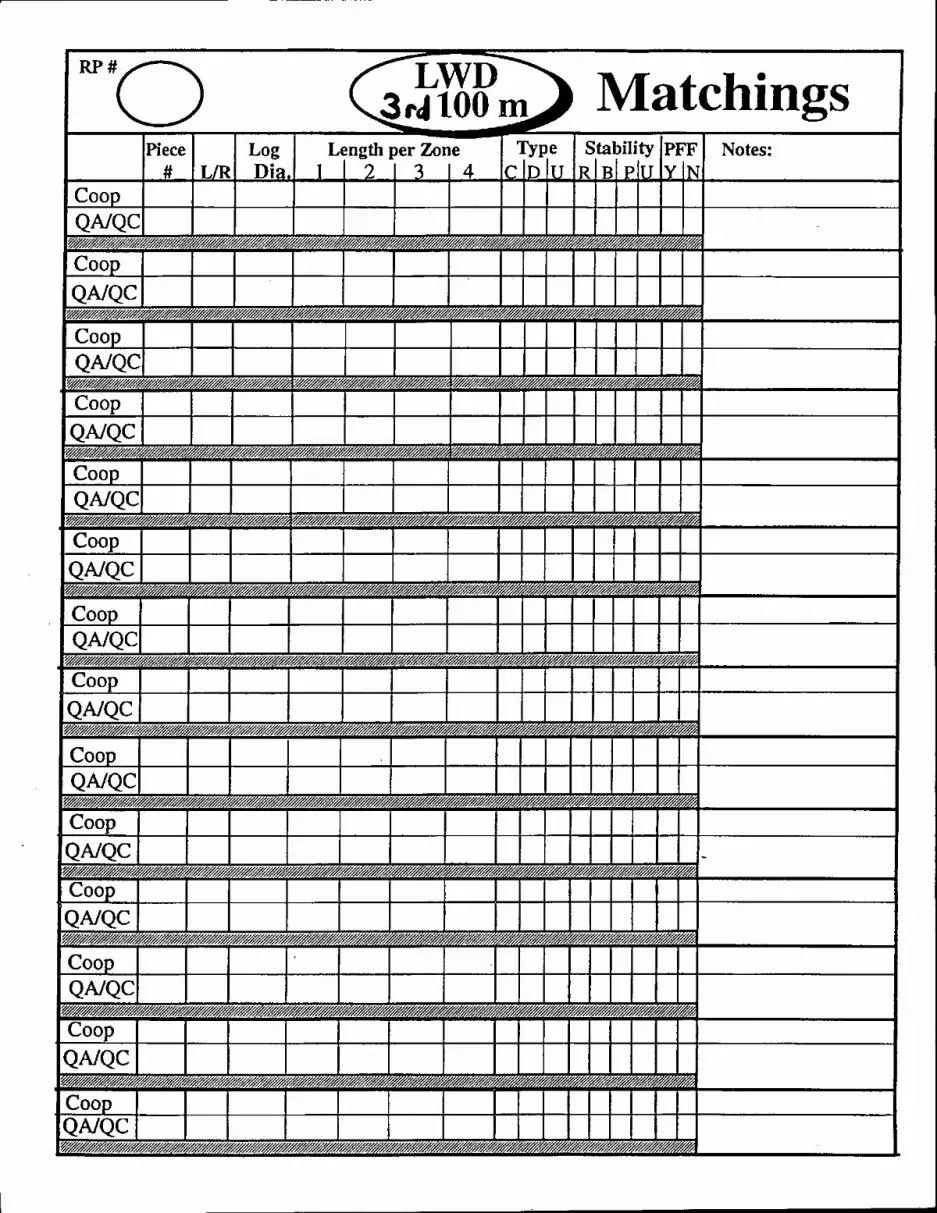
LWD rdl00 Matchings

Notes:

I APPENDIX E I TFW Ambient Monitoring Program

Salmonid Spawning Gravel Composition Module ****************SAMPLING****************

1994 QA Observation Field Survey

Date COOPERATOR COOP Crew

QAiQC Crew

Part A: Selection of the Sampling Reach

W.R.I.A. # Stream Segment # Grad. Rivermile to

BFW Conf.

1) Identifying a Sampling Segment {Salmonid use: cu"enJ, historic.!uture; GradienJ; Substrate size}

Is the chosen segment suitable according to protocol? (describe)' ________ _

2) Defining a Logistically Feasible Sampling Area {Site distribution; Access; Geomorphic Conditions}

Has the cooperator chosen sites within the segment that are accessible to crews? (describe) _________________________ _

3) Eliminating Areas in the Vicinity of In-stream Structures {Buffer zones for bridges, dmns, culverts}

How many were found in segment and was protocol followed? (describe) ____ _

4) Finalizing the Potential Sampling Reach How many potential sampling reaches did they end up with in segment and does it reflect steps 1-3? (describe) _____________________ _

5) Appropriateness of Time to Collect Samples {Stable substrate; Salmonid presence; Discharge regime}

When is the sampling being conducted? (describe) ____________ _

Summary

Part B: Identifying Potential Sampling Sites Within the Sampling Reach

1) Inventory of Riffle Crests

How many riffle crests where identified as potential sampling sites on this segment? riffle crests.

Did the cooperator. select riffle crests {geomorplwlogy, substrate comp.] which meet criteria? (describe) __________________________ _

Did the cooperator flag/mark the sampling sites properly? (describe), _____ _

2) Systematic Sampling Strategy

Did the cooperator develop a sampling strategy based on prior data available on this stream? (describe) _________________________ _

Did the cooperator follow the systematic strategy properly? (describe) Total # RCs__ Sequencing _____________ _ Random # Other ________________ _

Summary

Part C: Site Sampling of Individual Rime Crests

1) Equipment Checklist and condition/usefulness [good!jairlpoorJ Map delineating stream segments McNeil sampler with plunger Plastic buckets with secure lids numbered clearly Backpack carrier Squirt Bottles Bucket labels Field notebook Pencils Hip boots or chest waders Flagging Permanent markers Fiberglass tape

2) Identifying Sampling Points at Riffle Crests Total # Res Observed __ _ Tape over RC yes, _________ no _______ _ Spawning gravel edge yes' _________ 00 _______ _ 1/2 and 2/3 protocol yes' ________ no ______ _ Discard protocol yes _________ 0o, _______ _ Nores ____________________________ _

3) Collecting Samples with the McNeil Gravel Sampler Step 1 . McNeil Sampler Total # Samples Observed __ _

Pre-rinse yes 0o ______ _ Dwnstrrn Approach yes 0o, ______ _ Insertion Protocol yes 00 ______ _ Proper insertion yes no ______ _ Discard protocol yes 00'--_____ _ Notes __________________________ _

Step 2 • Sample Removal Hand layer method yes 00

Collection Basin yes no Stop-ring protocol yes no Hand rinse yes 00

Discard protocol yes no Notes

Step 3 - Plunger Clean plunger Insertion protocol Discard protocol

y~,--------------

y~,--------------

y~--------

no, ______________ __ no~ ____________ __ no, ______________ __

Notes ____________________________________________________ _

Step 4 - Rerrwval Sample bucket pre-rinse y~, ______________ no, ______________ _ Sample bucket stability y~ no, ______________ _ McNeil removal protocol yes no, ______________ _ Rinse y~ no, ______________ _ Discard protocol y~ no, ______________ _ Notes ____________________________________________________ _

Step 5 - Sample Bucket label Label y~, ________ _ no, ______________ _ Information y~, ______________ __ no, ______________ _ Sealing bucket yes, _____________ _ no, ____________ _ Nores ____________________________________________________ _

Summary

g:'qa-fonns'qased94.wp

I APPENDIX F I TFW Ambient MonitoringProgram

Salmonid Spawning Gravel Composition Module ***********VOLUMETRIC ANAL YSIS***********

1994 QA Observation Field Survey

Date COOPERATOR COOP Crew

QAlQC Crew

W.R.I.A. # Streain Segment # Grad. Rivermile to

BFW Conf.

Part A Documentation and Equipment Checklist

Data Form: Was the header infonnation filled out properly? yes ___ no

Sieves sieve diameter __ 64.0 mm mm Sieve holder Catch basin 32.0 mm mm Stand Water Supply 16.0 mm mm Tubing Connection

8.0 mm mm Mod. Graduated Cylinder 4.0 mm mm 2.0 mm mm Displacement Flask & valve 1.0 mm mm Grad. Cyl. -1000/500/100ml 0.85 mm mm Small cup Timers (3) 0.5 mm mm Data Fonns Pencils 0.25 mm mm Rain Gear Wire brush 0.125mm mm

Nores: ________________________________ ___

Part B Washing Gravel Through Sieves Total # Samples Observed

Step 1 - Filling Out Data Form 1 Form/day/segment Header Infonnation Sieve Sizes Notes

yes ______________ __ no __________ _ yes ______________ __ no __________ _ yes ______________ _ no __________ _

Step 2 - Processing Station Preparation Catch Basin DrainlRinse yes, ________ _ Mod. Grad. Cyl. yes, _______ _ Notes

Step 3 - Sieve Preparation Sieve Holder Stack Sieves Notes

ses _______ _ yes ________ _

Step 4 - Sample Data Recording yes, ________ _ Notes

Step 5 - Bucket Dump & Rinse yes, ________ _ Notes

Step 6 - Station Protocol Shake Protocol yes Wash Protocol yes Thoroughness

Large yes Medium yes Fines yes

Sieve Removal yes Sieve Holder Rinse yes

. Sieve Drying yes Discard Protocol yes Notes

Step 7 - Sieve Settling and Draining Time 15 min Sieves yes _______ --20 min Grad. Cyl. (on) yes, _______ _ 60 min Grad. Cyl. (off) yes _______ _ Notes

Summary

no, ______ _ no, ______ _

no ______ _ no ______ _

no, _____ _

no, _____ _

no no

no no no no no no no

no, ______ _ no, ______ _ no, ______ _

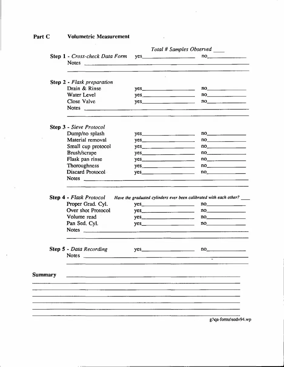
Part C Volumetric Measurement

Total # Samples Observed __ Step 1 - Cross-check Data Form yes _______ _ no, ______ _

Notes

Step 2 - Flask preparation Drain & Rinse yes, ________ _ no _____ _ Water Level yes, ________ _ no ______ _ Close Valve yes, _______ _ no ______ _

Notes

Step 3 - Sieve Protocol Dump/no splash yes no Material removal yes no Small cup protocol yes no Brush/scrape yes no Flask pan rin se yes no Thoroughness yes no Discard Protocol yes no Notes

Step 4 - Flask Protocol Proper Grad. Cyl. Over shot Protocol Volume read

Have the graduated cylinders ever been calibrated with each other? __

Pan Sed. Cyl. Notes

Step 5 - Data Recording Notes

yes no, _____ _ yes no, ______ _ yes _______ _ no, ______ _ yes _______ _ no, _____ _

yes _______ _ no, ______ _

Summary

g:'qa-fonns\5cdv94.wp

,------------------------------------------------

APPENDIXG


Stream Temperature Survey Module 1994 QA Observation Field Survey

- Not Available at this Time -

.-~~~~~~~~~------------------- -- ---

APPENDIXH Copy =< to Coop


QA Survey Report

Date Attended by Cooperator Site Trainers -

('Lead)

Modules o Stream Segment o Habitat Unit 0 Spawning Gravel Covered o Reference Point o Large Woody Debris 0 Stream Temperature

Summary

Stream/Site Description:

Equipment and Calibration:

Logistical Factors:

Survey Summm:ylRecommendatiolls:

TFWNotc: One of the TFW Ambient Monitoring Program's main quality assurance objectives is to continu-ally improve our methods and services through adaptive management. We encourage all Cooperators to share their opinions and experience on how this program can better meet their needs.

-

.. Northwest Indian Fisheries ComnllsslOn. 6730 Martin Way E .• OlympIa. W A 98S06 (206)438~ 1180 g:lqa-fonnsVptqa.pt4

QA Report (cont.)

Northwest Indian Fisheries Commission. 6730 Martin Way E ..• Olympia. WA 98506 (206)438-1180 g:\qa-fonm\rptqa.pt4

Documents

1994 ambient monitoring program manual - WA - DNR