ERDC

/CRR

ELM

P-22

-3

Dynamics Modeling and Robotic-Assist, Leader-Follower Control of Tractor Convoys

Cold

Regi

ons

Rese

arch

and

Engi

neer

ing

Labo

rato

ry

Joshua T. Cook, Laura E. Ray, and James H. Lever February 2022

Approved for public release; distribution is unlimited.

The U.S. Army Engineer Research and Development Center (ERDC) solves the nation’s toughest engineering and environmental challenges. ERDC develops innovative solutions in civil and military engineering, geospatial sciences, water resources, and environmental sciences for the Army, the Department of Defense, civilian agencies, and our nation’s public good. Find out more at www.erdc.usace.army.mil.

To search for other technical reports published by ERDC, visit the ERDC online library at https://erdclibrary.on.worldcat.org/discovery.

ERDC/CRREL MP-22-3 February 2022

Dynamics Modeling and Robotic-Assist, Leader-Follower Control of Tractor Convoys

Joshua T. Cook and Laura E. Ray

Thayer School of Engineering Dartmouth College 14 Engineering Drive Hanover, NH 03775

James H. Lever

Cold Regions Research and Engineering Laboratory U.S. Army Engineer Research and Development Center 72 Lyme Road Hanover, NH 03775

Final report

Approved for public release; distribution is unlimited.

Prepared for National Aeronautics and Space Administration Washington, DC 20546

Under NASA grant NNX-10AL97H

ERDC/CRREL MP 22-3 ii

Preface

This study was conducted for the National Aeronautics and Space Admin-istration (NASA) under NASA grant NNX-10AL97H.

The work was performed by the U.S. Army Engineer Research and Devel-opment Center, Cold Regions Research Engineering Laboratory (ERDC-CRREL) and Dartmouth College. At the time of publication of this paper, the deputy director for ERDC-CRREL was Mr. Bryan E. Baker and the director was Dr. Joseph Corriveau.

This article was originally published online in the Journal of Terra- mechanics on 27 June 2017.

COL Teresa A. Schlosser was the ERDC commander, and the director was Dr. David W. Pittman.

DISCLAIMER: The contents of this report are not to be used for advertising, publication, or promotional purposes. Citation of trade names does not constitute an official endorsement or approval of the use of such commercial products. All product names and trademarks cited are the property of their respective owners. The findings of this report are not to be construed as an official Department of the Army position unless so designated by other authorized documents.

DESTROY THIS REPORT WHEN NO LONGER NEEDED. DO NOT RETURN IT TO THE ORIGINATOR.

Dynamics modeling and robotic-assist,

leader-follower control of tractor convoys

Abstract

This paper proposes a generalized dynamics model and a leader-follower control architecture for skid-steered tracked vehicles towingpolar sleds. The model couples existing formulations in the literature for the powertrain components with the vehicle-terrain interactionto capture the salient features of terrain trafficability and predict the vehicles response. This coupling is essential for making realisticpredictions of the vehicles traversing capabilities due to the power-load relationship at the engine output. The objective of the modelis to capture adequate fidelity of the powertrain and off-road vehicle dynamics while minimizing the computational cost for model baseddesign of leader-follower control algorithms. The leader-follower control architecture presented proposes maintaining a flexible forma-tion by using a look-ahead technique along with a way point following strategy. Results simulate one leader-follower tractor pair wherethe leader is forced to take an abrupt turn and experiences large oscillations of its drawbar arm indicating potential payload instability.However, the follower tractor maintains the flexible formation but keeps its payload stable. This highlights the robustness of the pro-posed approach where the follower vehicle can reject errors in human leader driving.� 2017 ISTVS. Published by Elsevier Ltd. All rights reserved.

1. Introduction

Tracked vehicles have superior mobility in soft terrainwhen compared with other types of locomotion. This isbecause the vehicle’s weight is distributed over a large areawhich reduces sinkage and increases traction. The demandfor autonomous vehicle systems in soft terrain environ-ments is growing in agriculture, mining, construction andlogistics operations. In all of these domains, a heavy dutyvehicle is required to operate on a variety of terrains andis pulling or pushing a large payload. Under these circum-stances, autonomous systems must account for powertrain

dynamics and the terrain-track interaction. These factorshave a significant effect on the vehicle dynamics and pay-load stability due to terrain shearing failure. Most of theliterature for autonomous tracked vehicles addressesunloaded vehicles where powertrain capabilities and limita-tions are discounted. Kitano and Murakami conductedmodeling studies on unloaded tracked vehicles to evaluatetracked vehicle dynamics and turning stability using trackspeeds as model inputs discounting all powertrain effects(Kitano and Jyozaki, 1976; Kitano and Kuma, 1977;Eiyo and Kitano, 1984; Murakami et al., 1992). Le et al.makes the same modeling assumptions (Le et al., 1997).Ferretti modeled an agricultural tracked vehicle using dri-ver torques as model inputs but no powertrain model is dis-cussed (Ferretti and Girelli, 1999). Rubinstein developed avehicle model including powertrain components, but the

Nomenclature

A nominal ground contact area ð2:97 m2ÞB force vectorb lateral center to center track distance (2.98 m)c terrain cohesion (kPa)DLA look-ahead distance (m)DM Hydraulic Motor Displacement

ð105� 10�6 m3=radianÞDP Hydraulic Pump Displacement ðm3=radianÞDP ;Max Maximum Hydraulic Pump Displacement

ð120� 10�6 m3=radianÞF track traction force (N)F L left track traction force (N)F R right track traction force (N)gFD final drive gear ratiogGR transmission gear ratiogP hydraulic steering pump gear ratiogST hydraulic steering motor gear ratioHG angular momentum about body C.G.

ðkg �m2=sÞHL left driver angular momentum ðkg �m2=sÞHR right driver angular momentum ðkg �m2=sÞHT tractor angular momentum ðkg �m2=sÞHSD sled angular momentum ðkg �m2=sÞH angular momentum ðkg �m2=sÞhq coefficient of lateral resistance offset 0.3004i track slip ratio (%)iL left track slip ratio (%)iR right track slip ratio (%)JS driver and track moment of inertia about the j1

axis ð300 kg �m2ÞJT tractor moment of inertia about the k1 axis

ð1:5� 105 kg �m2ÞJSD sled moment of inertia about the k3 axis

ð3:98� 106 kg �m2ÞJe engine moment of inertia ð15 kg �m2ÞJ t transmission moment of inertia ð150 kg �m2ÞKdc transfer function dc gain ððm=sÞ�1ÞKi;v integral heading controller gain (deg/deg)Ki;v integral speed controller gain ððm=sÞ�1ÞKp;h proportional heading controller gain (deg/deg)Kp;v proportional speed controller gain ððm=sÞ�1Þk speed reference gain (m/s)K terrain shear deformation modulus (cm)kc modulus of terrain cohesion (kPa)kU modulus of terrain friction angle (deg)LA drawbar length (1 m)LSD sled length (21 m)LTA tractor CG to drawbar distance (0.82 m)LTA tractor CG to drawbar distance (1 m)l nominal track ground contact length (3.25 m)LTS rigid truss length (6 m)M mass matrixmB bladder mass (10,000 kg)

mT tractor mass (25,000 kg)mSD sled mass (80,000 kg)mq slope coefficient of lateral resistance (�0.0433)n modulus of terrain exponentPE engine power (kW)Ph pressure in h section of hose (Pa)Qh hydraulic fluid flow in the h section of hose

ðm3=sÞQj jth generalized forceqj jth generalized coordinateR track resistance force (N)RL longitudinal left track resistance force (N)RR longitudinal left track resistance force (N)Rc terrain compaction resistance (N)RSD;X sled resistance force in i3 direction (N)RSD;Y sled resistance force in j3 direction (N)RlLF lateral resistance force, left track, front section

(N)RlLR lateral resistance force, left track, rear section

(N)RlRF lateral resistance force, right track, front section

(N)RlRR lateral resistance force, right track, rear section

(N)RA=B rotation transformation from frame B to As laplace transform variableSD sledT kinetic energy (J)V h volume of h section of hose 6.6 � 10�3m3

rP=O position vector from point O to P (m)rSD=T position vector from the tractor C.G. to the sled

C.G. (m)rT=O position vector from the inertial frame origin to

tractor C.G. (m)v velocity (m/s)vG velocity of body C.G. (m/s)vT velocity of tractor (m/s)vSD velocity of sled (m/s)vx tractor i1 velocity (m/s)vy tractor j1 velocity (m/s)vleader leader vehicle velocity (m/s)vref controller reference velocity (m/s)W normal load of track segment on terrain (N)WP way pointX I tractor position in inertial frame (m)x state vectorxe follower longitudinal offset error (m)Y J tractor position in inertial frame (m)z track sinkage (m)a steering angle (deg)b hydraulic fluid bulk modulus ð2:79� 109 PaÞv engine throttle dilationd transfer function time constant (s)

2

dt gear shift time constant (0.25 s)g sled resistance coefficient (0.11)C normalized wet friction clutch command (N�m)k wet friction clutch viscous coefficient ð1 s�1ÞlS lateral resistance coefficient based on z

ð10 kg �m2=sÞX engine speed (RPM)x angular velocity (rad/s)xL left track or driver angular velocity (rad/s)xR right track or driver angular velocity (rad/s)xE engine speed (rad/s)xt;in transmission rotational input shaft speed (rad/s)xt;out transmission rotational output shaft speed (rad/

s)U terrain friction angle (rad)P normalized engine throttle command/ drawbar orientation relative to frame 1 (rad)w sled orientation relative to frame 1 (rad)uL left track or driver angular position (rad)uR right track or driver angular position (rad)

q radius of curvature (rad)sE;Max maximum available engine torque at a given en-

gine speed (N�m)sL left track or drive torque (N�m)sM hydraulic motor output torque (N�m)sP hydraulic pump load torque on engine (N�m)sR right track or drive torque (N�m)sf ;d wet friction clutch dynamic torque (Nm)sf ;max;d wet friction clutch maximum dynamic torque

threshold (1800 Nm)sf ;max;s wet friction clutch maximum static torque

threshold (2200 Nm)sf ;s wet friction clutch static torque (Nm)st;in transmission input torque (N�m)st;out transmission output torque (N�m)h tractor orientation in the inertial frame (rad)f track or driver damping coefficient

ð10 kg �m2=sÞfe engine damping coefficient ð1 kg �m2=sÞft transmission damping coefficient ð10 kg �m2=sÞ

3

terrain-track interaction fidelity is beyond the requirementsfor control law development, and no payload is present(Rubinstein and Hitron, 2004).

In this paper we have developed a comprehensivetracked vehicle model for numerical experiments withautonomous tractors. The model encompasses all the ofthe salient features that significantly effect the vehicle’sdynamics under load on deformable terrain in a simulationtest bed while minimizing the computational cost. Thesesalient features are the driver inputs, the powertrain model,Wong terramechanics theory that adequately captures theterrain-track interaction, the relationship between a givenpayload and the load it places on the vehicle drawbar,and multi-body dynamics. These features are all coupledtogether as the powertrain puts limitations on the vehicle’scapabilities due to the terrain-vehicle interaction and pay-load. The model’s balance between fidelity and computa-tional cost makes it a powerful tool for iterative modelbased design for general purpose unmanned tractor sys-tems and their controller designs due to fast simulationtimes.

The work is motivated by the US Antarctic Program’s(USAP) South Pole Traverse (SPT) which resupplies theNational Science Foundation’s South Pole Research Sta-tion from McMurdo Station. Presently, traverse operationsuse two fleets for two round trips each season where eachfleet consists of eight tractors and an eight-person crew.These trips via ground offset the number of LC130 flightsrequired to transport cargo and fuel providing an economicbenefit of $2 M per trip. Each trip currently takes 50 daysbut if an effective manned leader, autonomous followerrobotic assist technology can be deployed, further savingscan be unlocked by reducing this round trip time to allow

for increased ground transport. The current towing config-uration uses polar sleds that are most commonly loadedwith fuel bladders (Lever and Weale, 2012). The low resis-tance forces between the sled and snow allow tractors topull large payloads (80,000 kg). However, autonomoustractors equipped with polar sleds raises concerns of pay-load stability as the payload is free to swing about thedrawbar. Furthermore, the Antarctic continent provides aunique challenge for implementation as there are largeamounts of spatial and temporal terrain variation due tounpredictable weather and snowfall. The variation in ter-rain can significantly impact the vehicle dynamics, mobil-ity, and payload stability. The model allows forexhaustive numerical experiments to test controllers andautomation strategies across different payloads, the vehi-cle’s bounded state space, and the terrain parameter space.

The manned leader, autonomous follower robotic assistapproach proposed in this paper is limited to a single fol-lower although it can readily be applied to multiple follow-ers. Emphasis is placed on maintaining a flexible formationrather than focusing on the follower’s convergence to a ref-erence trajectory (Barfoot and Clark, 2004; Low, 2015).This allows the follower to use its leader’s trajectory as aguide rather than a strict reference input so that humanerror in driving is rejected for robust payload stability. Thisis done using a look-ahead approach with a sequence ofway points as a guide that are user defined offsets of the lea-der’s path. It is assumed that communication between vehi-cles and accurate measurements of vehicle GPS position,speed, and heading update at 10 Hz. These rates are basedon autonomous tractor hardware used in Zhang et al.(2009). Simulation results demonstrate the effectiveness ofthe proposed approach.

4

The remainder of the paper is organized as follows: Sec-tion 2 goes over the tractor-sled towing configuration as itrelates to the assumptions for the Lagrange multi-bodydynamics derivation, Bekker-Wong terramechanics, andthe powertrain model. Section 3 goes over in detail the pro-posed leader-follower control strategy. Section 4 showssimulation results and demonstrates the robustness of theproposed control approach.

2. Dynamics modeling

2.1. Tractor-sled configuration

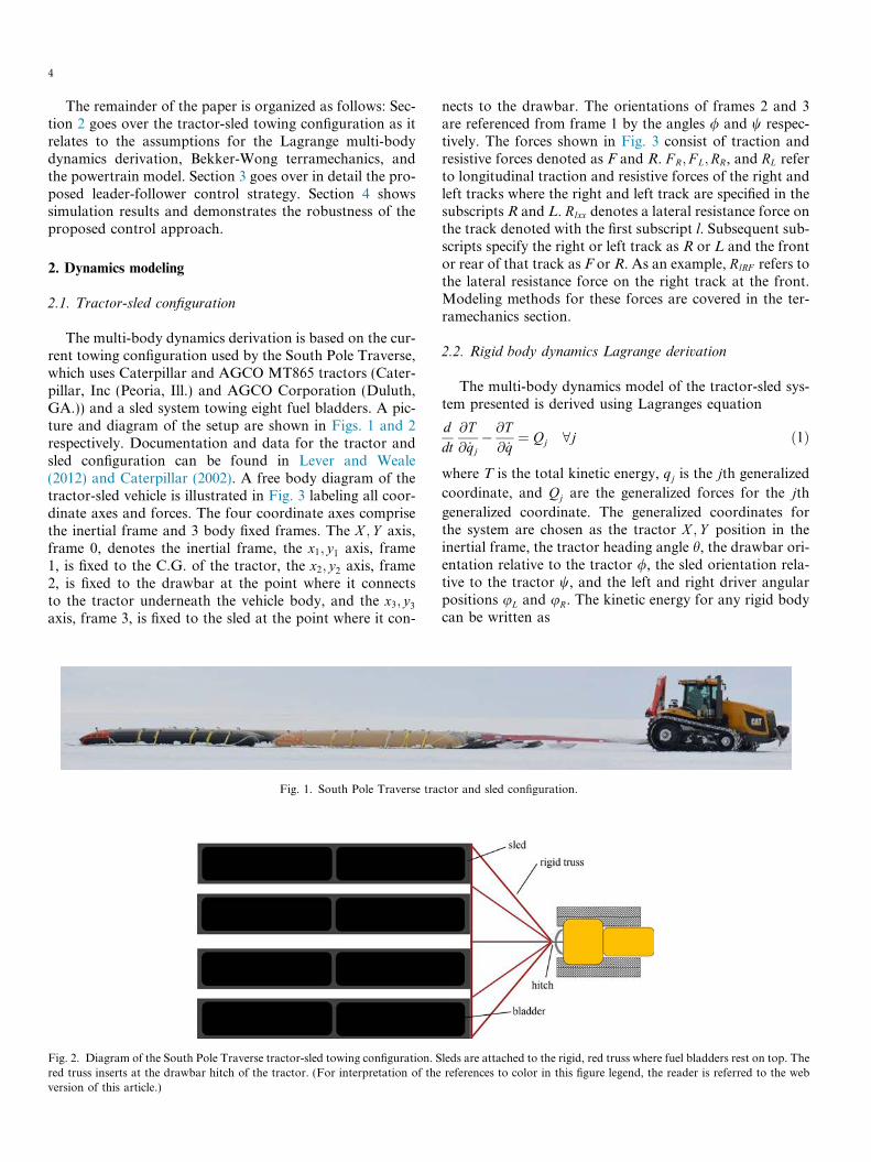
The multi-body dynamics derivation is based on the cur-rent towing configuration used by the South Pole Traverse,which uses Caterpillar and AGCO MT865 tractors (Cater-pillar, Inc (Peoria, Ill.) and AGCO Corporation (Duluth,GA.)) and a sled system towing eight fuel bladders. A pic-ture and diagram of the setup are shown in Figs. 1 and 2respectively. Documentation and data for the tractor andsled configuration can be found in Lever and Weale(2012) and Caterpillar (2002). A free body diagram of thetractor-sled vehicle is illustrated in Fig. 3 labeling all coor-dinate axes and forces. The four coordinate axes comprisethe inertial frame and 3 body fixed frames. The X ; Y axis,frame 0, denotes the inertial frame, the x1; y1 axis, frame1, is fixed to the C.G. of the tractor, the x2; y2 axis, frame2, is fixed to the drawbar at the point where it connectsto the tractor underneath the vehicle body, and the x3; y3axis, frame 3, is fixed to the sled at the point where it con-

Fig. 1. South Pole Traverse tra

Fig. 2. Diagram of the South Pole Traverse tractor-sled towing configuration. Sred truss inserts at the drawbar hitch of the tractor. (For interpretation of theversion of this article.)

nects to the drawbar. The orientations of frames 2 and 3are referenced from frame 1 by the angles / and w respec-tively. The forces shown in Fig. 3 consist of traction andresistive forces denoted as F and R. F R; F L;RR, and RL referto longitudinal traction and resistive forces of the right andleft tracks where the right and left track are specified in thesubscripts R and L. Rlxx denotes a lateral resistance force onthe track denoted with the first subscript l. Subsequent sub-scripts specify the right or left track as R or L and the frontor rear of that track as F or R. As an example, RlRF refers tothe lateral resistance force on the right track at the front.Modeling methods for these forces are covered in the ter-ramechanics section.

2.2. Rigid body dynamics Lagrange derivation

The multi-body dynamics model of the tractor-sled sys-tem presented is derived using Lagranges equation

ddt

@T@ _qj

� @T@ _q

¼ Qj 8j ð1Þ

where T is the total kinetic energy, qj is the jth generalized

coordinate, and Qj are the generalized forces for the jthgeneralized coordinate. The generalized coordinates forthe system are chosen as the tractor X ; Y position in theinertial frame, the tractor heading angle h, the drawbar ori-entation relative to the tractor /, the sled orientation rela-tive to the tractor w, and the left and right driver angularpositions uL and uR. The kinetic energy for any rigid bodycan be written as

ctor and sled configuration.

leds are attached to the rigid, red truss where fuel bladders rest on top. Thereferences to color in this figure legend, the reader is referred to the web

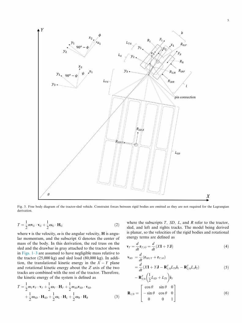
Fig. 3. Free body diagram of the tractor-sled vehicle. Constraint forces between rigid bodies are omitted as they are not required for the Lagrangianderivation.

5

T ¼ 1

2mvG � vG þ 1

2xG �HG ð2Þ

where v is the velocity, x is the angular velocity, H is angu-lar momentum, and the subscript G denotes the center ofmass of the body. In this derivation, the red truss on thesled and the drawbar in gray attached to the tractor shownin Figs. 1–3 are assumed to have negligible mass relative tothe tractor (25,000 kg) and sled load (80,000 kg). In addi-tion, the translational kinetic energy in the X � Y planeand rotational kinetic energy about the Z axis of the twotracks are combined with the rest of the tractor. Therefore,the kinetic energy of the system is defined as

T ¼ 1

2mT vT � vT þ 1

2xT �HT þ 1

2mSDvSD � vSD

þ 1

2xSD �HSD þ 1

2xL �HL þ 1

2xR �HR ð3Þ

where the subscripts T ; SD; L, and R refer to the tractor,sled, and left and rights tracks. The model being derivedis planar, so the velocities of the rigid bodies and rotationalenergy terms are defined as

vT ¼ ddtrT=O ¼ d

dtðX Iþ Y JÞ ð4Þ

vSD ¼ ddtðrSD=T þ rT=OÞ

¼ ddtðX Iþ Y J� RT

1=0LTAi1 � RT2=0LAi2Þ

� RT3=0

1

2LSD þ LTS

� �i3

ð5Þ

R1=0 ¼cos h sin h 0

� sin h cos h 0

0 0 1

264

375 ð6Þ

6

R2=0 ¼cos/ sin/ 0

� sin/ cos/ 0

0 0 1

264

375R1=0 ð7Þ

R3=0 ¼cosw sinw 0

� sinw cosw 0

0 0 1

264

375R1=0 ð8Þ

1

2xG �HG ¼ 1

2JT

_h2 ð9Þ1

2xSD �HSD ¼ 1

2JSDð _hþ _wÞ2 ð10Þ

1

2xL �HL ¼ 1

2JS _u

2L ð11Þ

1

2xR �HR ¼ 1

2JS _u

2R ð12Þ

where LTA is the distance from the tractor CG to the draw-bar, LA is the drawbar length, LTS is the truss length, andLSD is the sled length. Rotational transformation matricesare generally defined as RA=B, where the rotation is fromframe B to frame A. From the definition of the kineticenergy, the full and partial derivatives can be taken onthe left side of Eq. (1) for all the generalized coordinates.The next step is to define the generalized forces, which dovirtual work through virtual displacements of the general-ized coordinates and are given by

Qj ¼XP

FP � @

@qjrP=O þ

XK

CK � @

@qjhK 8j ð13Þ

where FP is an arbitrary force vector that acts at rP=O andCK is an arbitrary torque vector acting on body K withan angular position hK . For the derivation of the tractor-sled system, the terms in Eq. (13) are evaluated as

XP

FP � @

@qjrP=O ¼ RT

1=0F Li1 � @

@qjrT=O þ RT

1=0

b2j1

� �

þ RT1=0F Ri1 � @

@qjrT=O � RT

1=0

b2j1

� �

� RT1=0RLi1 � @

@qjrT=O þ RT

1=0

l2i1 þ b

2j1

� �� �

� RT1=0RRi1 � @

@qjrT=O þ RT

1=0

l2i1 � b

2j1

� �� �

þ RT1=0RlLF j1 �

@

@qjrT=O þ RT

1=0

l2i1 þ b

2j1

� �� �

þ RT1=0RlRF j1 �

@

@qjrT=O þ RT

1=0

l2i1 � b

2j1

� �� �

þ RT1=0RlLRj1 �

@

@qjrT=O þ RT

1=0 � l2i1 þ b

2j1

� �� �

þ RT1=0RlRRj1 �

@

@qjrT=O þ RT

1=0 � l2i1 � b

2j1

� �� �

þ RT3=0 RSD;X i3 þ RSD;Y j3ð Þ � @

@qjrSD=T þ rT=O� �

ð14Þ

XK

CK � @

@qjhK ¼ sL � F Lr� f _uLð Þj1 �

@

@qjuLj1 þ hk1ð Þ

þ sR � F Rr� f _uRð Þj1 �@

@qjuRj1 þ hk1ð Þ ð15Þ

This derivation gives the differential equations for therigid body dynamics of the tractor sled system in terms

of €X and €Y . However, the motivation for the model isautonomous vehicle control, so we make substitutions torewrite the equations in terms of _vx and _vy correspondingto the longitudinal and lateral velocity of the tractor inframe 1. The velocity of the tractor can be written as

_X ¼ vx cos h� vy sin h ð16Þ_Y ¼ vy cos hþ vx sin h ð17Þand then differentiated

€X ¼ _vx cos h� _vy sin h� _hðvy cos hþ vx sin hÞ ð18Þ€Y ¼ _vy cos hþ _vx sin hþ _hðvx cos h� vy sin hÞ ð19Þ

Using Eqs. (18) and (19) for substitution, the equationsof motion can be written in terms of the body fixed tractorvelocities as _x ¼ f ðxÞ, where the state vector is defined inEq. (20).

x � X Y h / w vx vy _h _/ _w _uL _uR

� �Tð20Þ

_x ¼ M�1BðxÞ ð21ÞDefinitions for the mass matrix M7x7 and the force

vector B7x1 are given in Appendix A.

2.3. Terramechanics

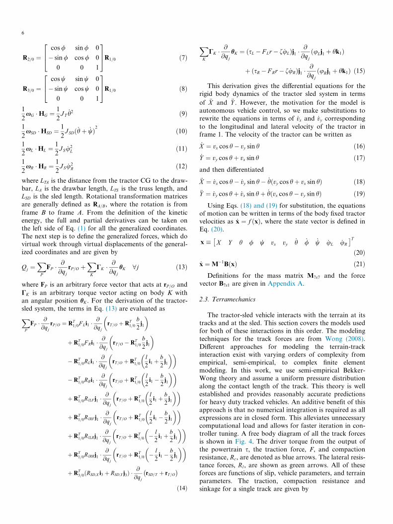
The tractor-sled vehicle interacts with the terrain at itstracks and at the sled. This section covers the models usedfor both of these interactions in this order. The modelingtechniques for the track forces are from Wong (2008).Different approaches for modeling the terrain-trackinteraction exist with varying orders of complexity fromempirical, semi-empirical, to complex finite elementmodeling. In this work, we use semi-empirical Bekker-Wong theory and assume a uniform pressure distributionalong the contact length of the track. This theory is wellestablished and provides reasonably accurate predictionsfor heavy duty tracked vehicles. An additive benefit of thisapproach is that no numerical integration is required as allexpressions are in closed form. This alleviates unnecessarycomputational load and allows for faster iteration in con-troller tuning. A free body diagram of all the track forcesis shown in Fig. 4. The driver torque from the output ofthe powertrain s, the traction force, F, and compactionresistance, Rc, are denoted as blue arrows. The lateral resis-tance forces, Rl, are shown as green arrows. All of theseforces are functions of slip, vehicle parameters, and terrainparameters. The traction, compaction resistance andsinkage for a single track are given by

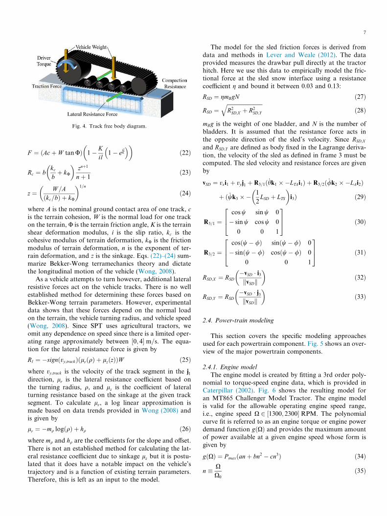
Fig. 4. Track free body diagram.

7

F ¼ ðAcþ W tanUÞ 1� Kil

1� eilK

� � �ð22Þ

Rc ¼ bkcbþ kU

� �znþ1

nþ 1ð23Þ

z ¼ W =Aðkc=bÞ þ kU

� �1=n

ð24Þ

where A is the nominal ground contact area of one track, cis the terrain cohesion, W is the normal load for one trackon the terrain, U is the terrain friction angle, K is the terrainshear deformation modulus, i is the slip ratio, kc is thecohesive modulus of terrain deformation, kU is the frictionmodulus of terrain deformation, n is the exponent of ter-rain deformation, and z is the sinkage. Eqs. (22)–(24) sum-marize Bekker-Wong terramechanics theory and dictatethe longitudinal motion of the vehicle (Wong, 2008).

As a vehicle attempts to turn however, additional lateralresistive forces act on the vehicle tracks. There is no wellestablished method for determining these forces based onBekker-Wong terrain parameters. However, experimentaldata shows that these forces depend on the normal loadon the terrain, the vehicle turning radius, and vehicle speed(Wong, 2008). Since SPT uses agricultural tractors, weomit any dependence on speed since there is a limited oper-ating range approximately between ½0; 4� m=s. The equa-tion for the lateral resistance force is given by

Rl ¼ �signðvy;trackÞðlrðqÞ þ lzðzÞÞW ð25Þwhere vy;track is the velocity of the track segment in the j1direction, lr is the lateral resistance coefficient based onthe turning radius, q, and lz is the coefficient of lateralturning resistance based on the sinkage at the given tracksegment. To calculate lr, a log linear approximation ismade based on data trends provided in Wong (2008) andis given by

lr ¼ �mq logðqÞ þ hq ð26Þwhere mq and hq are the coefficients for the slope and offset.There is not an established method for calculating the lat-eral resistance coefficient due to sinkage lz but it is postu-lated that it does have a notable impact on the vehicle’strajectory and is a function of existing terrain parameters.Therefore, this is left as an input to the model.

The model for the sled friction forces is derived fromdata and methods in Lever and Weale (2012). The dataprovided measures the drawbar pull directly at the tractorhitch. Here we use this data to empirically model the fric-tional force at the sled snow interface using a resistancecoefficient g and bound it between 0.03 and 0.13:

RSD ¼ gmBgN ð27ÞRSD ¼

ffiffiffiffiffiffiffiffiffiffiffiffiffiffiffiffiffiffiffiffiffiffiffiffiffiffiR2SD;X þ R2

SD;Y

qð28Þ

mBg is the weight of one bladder, and N is the number ofbladders. It is assumed that the resistance force acts inthe opposite direction of the sled’s velocity. Since RSD;X

and RSD;Y are defined as body fixed in the Lagrange deriva-tion, the velocity of the sled as defined in frame 3 must becomputed. The sled velocity and resistance forces are givenby

vSD ¼ vxi1 þ vy j1 þ R3=1ð _hk1 ��LTAi1Þ þ R3=2ð _/k2 ��LAi2Þ

þ ð _wk3 �� 1

2LSD þ LTS

� �i3Þ ð29Þ

R3=1 ¼cosw sinw 0

� sinw cosw 0

0 0 1

264

375 ð30Þ

R3=2 ¼cosðw� /Þ sinðw� /Þ 0

� sinðw� /Þ cosðw� /Þ 0

0 0 1

264

375 ð31Þ

RSD;X ¼ RSD�vSD � i3kvSDk

� �ð32Þ

RSD;Y ¼ RSD�vSD � j3kvSDk

� �ð33Þ

2.4. Power-train modeling

This section covers the specific modeling approachesused for each powertrain component. Fig. 5 shows an over-view of the major powertrain components.

2.4.1. Engine model

The engine model is created by fitting a 3rd order poly-nomial to torque-speed engine data, which is provided inCaterpillar (2002). Fig. 6 shows the resulting model foran MT865 Challenger Model Tractor. The engine modelis valid for the allowable operating engine speed range,i.e., engine speed X 2 ½1300; 2300� RPM. The polynomialcurve fit is referred to as an engine torque or engine powerdemand function gðXÞ and provides the maximum amountof power available at a given engine speed whose form isgiven by

gðXÞ ¼ Pmaxðanþ bn2 � cn3Þ ð34Þ

n � XX0

ð35Þ

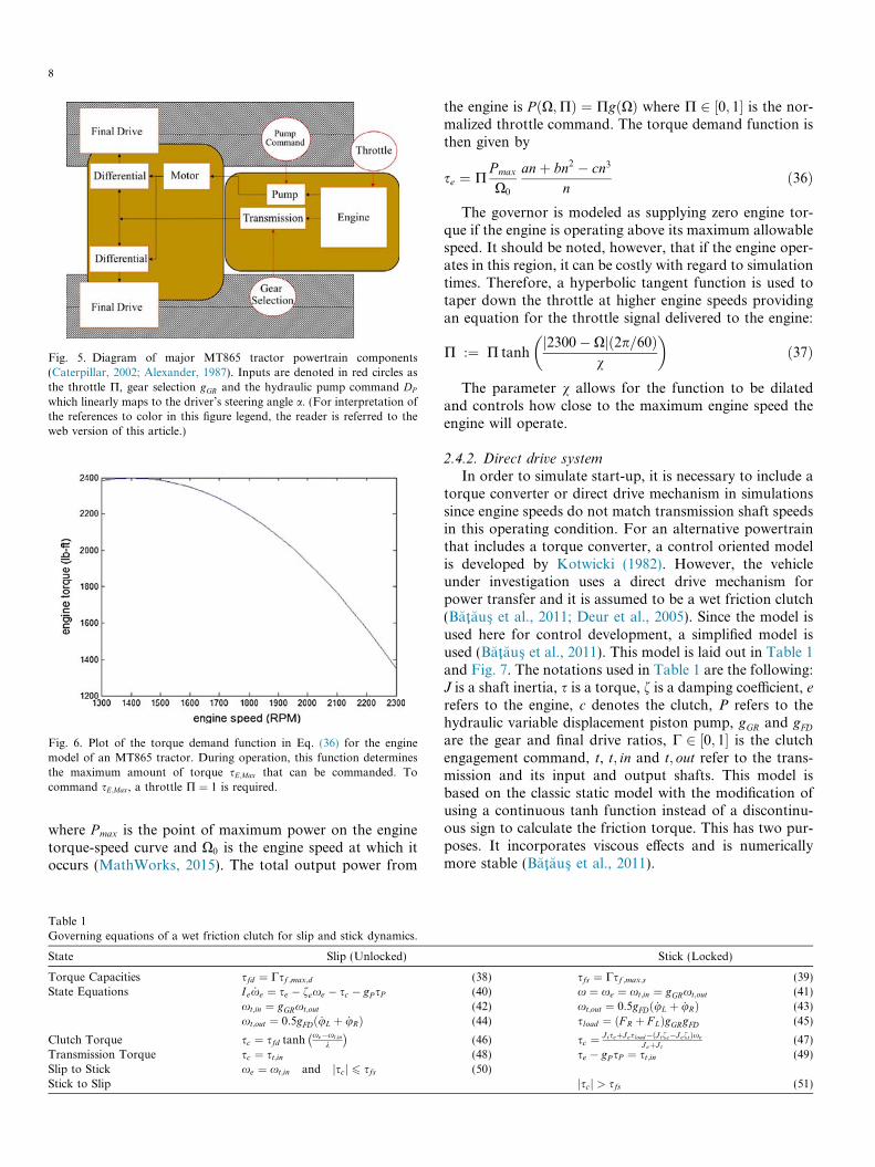
Fig. 5. Diagram of major MT865 tractor powertrain components(Caterpillar, 2002; Alexander, 1987). Inputs are denoted in red circles asthe throttle P, gear selection gGR and the hydraulic pump command DP

which linearly maps to the driver’s steering angle a. (For interpretation ofthe references to color in this figure legend, the reader is referred to theweb version of this article.)

Fig. 6. Plot of the torque demand function in Eq. (36) for the enginemodel of an MT865 tractor. During operation, this function determinesthe maximum amount of torque sE;Max that can be commanded. Tocommand sE;Max, a throttle P ¼ 1 is required.

8

where Pmax is the point of maximum power on the enginetorque-speed curve and X0 is the engine speed at which itoccurs (MathWorks, 2015). The total output power from

Table 1Governing equations of a wet friction clutch for slip and stick dynamics.

State Slip (Unlocked)

Torque Capacities sfd ¼ Csf ;max;d

State Equations Ie _xe ¼ se � fexe � sc � gP sPxt;in ¼ gGRxt;out

xt;out ¼ 0:5gFDð _uL þ _uRÞClutch Torque sc ¼ sfd tanh

xe�xt;in

k

� �Transmission Torque sc ¼ st;inSlip to Stick xe ¼ xt;in and jscj 6 sfsStick to Slip

the engine is P ðX;PÞ ¼ PgðXÞ where P 2 ½0; 1� is the nor-malized throttle command. The torque demand function isthen given by

se ¼ PPmax

X0

anþ bn2 � cn3

nð36Þ

The governor is modeled as supplying zero engine tor-que if the engine is operating above its maximum allowablespeed. It should be noted, however, that if the engine oper-ates in this region, it can be costly with regard to simulationtimes. Therefore, a hyperbolic tangent function is used totaper down the throttle at higher engine speeds providingan equation for the throttle signal delivered to the engine:

P :¼ P tanhj2300� Xjð2p=60Þ

v

� �ð37Þ

The parameter v allows for the function to be dilatedand controls how close to the maximum engine speed theengine will operate.

2.4.2. Direct drive system

In order to simulate start-up, it is necessary to include atorque converter or direct drive mechanism in simulationssince engine speeds do not match transmission shaft speedsin this operating condition. For an alternative powertrainthat includes a torque converter, a control oriented modelis developed by Kotwicki (1982). However, the vehicleunder investigation uses a direct drive mechanism forpower transfer and it is assumed to be a wet friction clutch(Bataus� et al., 2011; Deur et al., 2005). Since the model isused here for control development, a simplified model isused (Bataus� et al., 2011). This model is laid out in Table 1and Fig. 7. The notations used in Table 1 are the following:J is a shaft inertia, s is a torque, f is a damping coefficient, erefers to the engine, c denotes the clutch, P refers to thehydraulic variable displacement piston pump, gGR and gFDare the gear and final drive ratios, C 2 ½0; 1� is the clutchengagement command, t, t; in and t; out refer to the trans-mission and its input and output shafts. This model isbased on the classic static model with the modification ofusing a continuous tanh function instead of a discontinu-ous sign to calculate the friction torque. This has two pur-poses. It incorporates viscous effects and is numericallymore stable (Bataus� et al., 2011).

Stick (Locked)

(38) sfs ¼ Csf ;max;s (39)(40) x ¼ xe ¼ xt;in ¼ gGRxt;out (41)(42) xt;out ¼ 0:5gFDð _uL þ _uRÞ (43)(44) sload ¼ ðF R þ F LÞgGRgFD (45)

(46) sc ¼ J tseþJesload�ðJ tfe�JeftÞxe

JeþJ t(47)

(48) se � gP sP ¼ st;in (49)(50)

jscj > sfs (51)

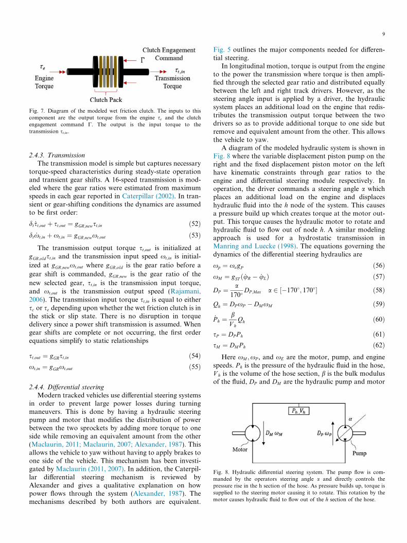
Fig. 7. Diagram of the modeled wet friction clutch. The inputs to thiscomponent are the output torque from the engine se and the clutchengagement command C. The output is the input torque to thetransmission st;in.

9

2.4.3. Transmission

The transmission model is simple but captures necessarytorque-speed characteristics during steady-state operationand transient gear shifts. A 16-speed transmission is mod-eled where the gear ratios were estimated from maximumspeeds in each gear reported in Caterpillar (2002). In tran-sient or gear-shifting conditions the dynamics are assumedto be first order:

dt _st;out þ st;out ¼ gGR;newst;in ð52Þdt _xt;in þ xt;in ¼ gGR;newxt;out ð53Þ

The transmission output torque st;out is initialized atgGR;oldst;in and the transmission input speed xt;in is initial-

ized at gGR;newxt;out where gGR;old is the gear ratio before a

gear shift is commanded, gGR;new is the gear ratio of the

new selected gear, st;in is the transmission input torque,and xt;out is the transmission output speed (Rajamani,2006). The transmission input torque st;in is equal to eithersc or se depending upon whether the wet friction clutch is inthe stick or slip state. There is no disruption in torquedelivery since a power shift transmission is assumed. Whengear shifts are complete or not occurring, the first orderequations simplify to static relationships

st;out ¼ gGRst;in ð54Þxt;in ¼ gGRxt;out ð55Þ

Fig. 8. Hydraulic differential steering system. The pump flow is com-manded by the operators steering angle a and directly controls thepressure rise in the h section of the hose. As pressure builds up, torque issupplied to the steering motor causing it to rotate. This rotation by themotor causes hydraulic fluid to flow out of the h section of the hose.

2.4.4. Differential steeringModern tracked vehicles use differential steering systems

in order to prevent large power losses during turningmaneuvers. This is done by having a hydraulic steeringpump and motor that modifies the distribution of powerbetween the two sprockets by adding more torque to oneside while removing an equivalent amount from the other(Maclaurin, 2011; Maclaurin, 2007; Alexander, 1987). Thisallows the vehicle to yaw without having to apply brakes toone side of the vehicle. This mechanism has been investi-gated by Maclaurin (2011, 2007). In addition, the Caterpil-lar differential steering mechanism is reviewed byAlexander and gives a qualitative explanation on howpower flows through the system (Alexander, 1987). Themechanisms described by both authors are equivalent.

Fig. 5 outlines the major components needed for differen-tial steering.

In longitudinal motion, torque is output from the engineto the power the transmission where torque is then ampli-fied through the selected gear ratio and distributed equallybetween the left and right track drivers. However, as thesteering angle input is applied by a driver, the hydraulicsystem places an additional load on the engine that redis-tributes the transmission output torque between the twodrivers so as to provide additional torque to one side butremove and equivalent amount from the other. This allowsthe vehicle to yaw.

A diagram of the modeled hydraulic system is shown inFig. 8 where the variable displacement piston pump on theright and the fixed displacement piston motor on the lefthave kinematic constraints through gear ratios to theengine and differential steering module respectively. Inoperation, the driver commands a steering angle a whichplaces an additional load on the engine and displaceshydraulic fluid into the h node of the system. This causesa pressure build up which creates torque at the motor out-put. This torque causes the hydraulic motor to rotate andhydraulic fluid to flow out of node h. A similar modelingapproach is used for a hydrostatic transmission inManring and Luecke (1998). The equations governing thedynamics of the differential steering hydraulics are

xp ¼ xegP ð56ÞxM ¼ gST ð _uR � _uLÞ ð57ÞDP ¼ a

170�DP ;Max a 2 ½�170�; 170�� ð58Þ

Qh ¼ DPxP � DMxM ð59Þ_Ph ¼ b

V hQh ð60Þ

sP ¼ DPPh ð61ÞsM ¼ DMPh ð62Þ

Here xM ;xP , and xE are the motor, pump, and enginespeeds. Ph is the pressure of the hydraulic fluid in the hose,V h is the volume of the hose section, b is the bulk modulusof the fluid, DP and DM are the hydraulic pump and motor

10

displacements, gST is the gear ratio between the hydraulicmotor and drivers, and sP and sM are the load torque onthe engine from the pump and the torque output fromthe motor. It should be noted that the flow out of the pumpis explicitly commanded by the operator via steering anglea and the flows out of the pump and into the motor are notequivalent unless the hydraulic pressure Ph is at a constantoperating value. The torques delivered to the drivers ateach track are

sR ¼ 1

2st;out þ 1

2sMgST ð63Þ

sL ¼ 1

2st;out � 1

2sMgST ð64Þ

3. Leader follower control

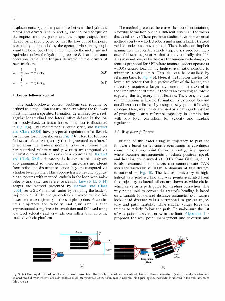
The leader-follower control problem can roughly bedefined as a regulation control problem where the followermust maintain a specified formation determined by a rect-angular longitudinal and lateral offset defined in the lea-der’s body-fixed, cartesian frame. This idea is illustratedin Fig. 9(a). This requirement is quite strict, and Barfootand Clark (2004) have proposed regulation of a flexiblecurvilinear formation shown in Fig. 9(b). Here the followerfollows a reference trajectory that is generated as a lateraloffset from the leader’s nominal trajectory where timeparameterized velocities and yaw rates are computed viakinematic constraints in curvilinear coordinates (Barfootand Clark, 2004). However, the leaders in this study arealso unmanned so these nominal trajectories are absentfrom noise and disturbances since they are computed viaa higher level planner. This approach is not readily applica-ble to systems with manned leader’s in the loop with noisyvelocity and yaw rate reference signals. Low (2015, 2014)adapts the method presented by Barfoot and Clark(2004) for a SUV manned leader by sampling the leader’strajectory at 20 Hz and generating a tracked vehicle fol-lower reference trajectory at the sampled points. A contin-uous trajectory for velocity and yaw rate is thenapproximated using linear interpolation and followed usinglow level velocity and yaw rate controllers built into thetracked vehicle platform.

Fig. 9. (a) Rectangular coordinate leader follower formation. (b) Flexible, curcolored red, follower tractors are colored blue. (For interpretation of the referenthis article.)

The method presented here uses the idea of maintaininga flexible formation but in a different way than the worksdiscussed above These previous studies have implementedmethods on two wheeled robots and a much lighter trackedvehicle under no drawbar load. There is also an implicitassumption that leader vehicle trajectories produce refer-ence follower trajectories that are dynamically feasible.This may not always be the case for human-in-the-loop sys-tems as proposed for SPT where manned leaders operate at�100% engine load in the highest gear ratio possible tominimize traverse times. This idea can be visualized byreferring back to Fig. 9(b). Here, if the follower tractor fol-lows a trajectory that is a perfect offset of the leader, thistrajectory requires a larger arc length to be traveled inthe same amount of time. If there is no extra engine torquecapacity, this trajectory is not feasible. Therefore, the ideaof maintaining a flexible formation is extended beyondcurvilinear coordinates by using a way point followingstrategy. Here, way points are used as a path guide insteadof providing a strict reference trajectory in combinationwith low level controllers for velocity and headingregulation.

3.1. Way point following

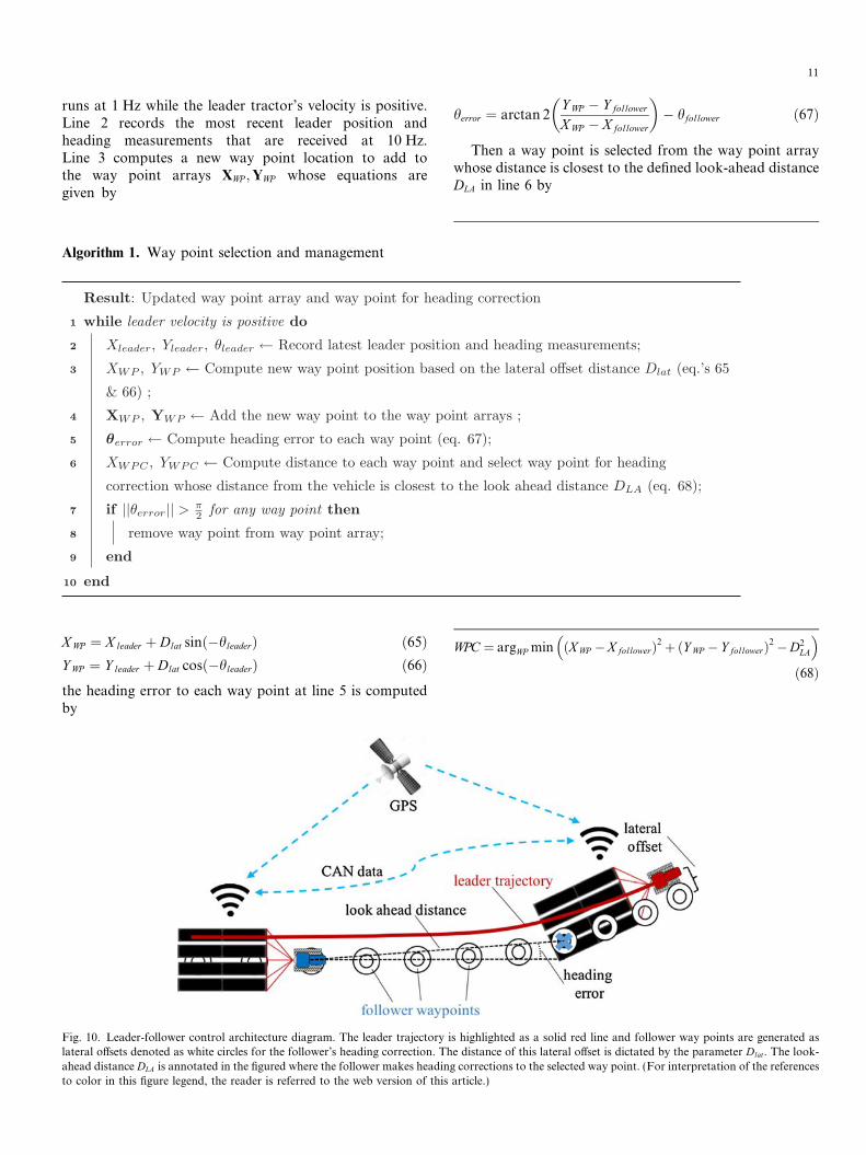
Instead of the leader using its trajectory to plan thefollower’s based on kinematic constraints in curvilinearcoordinates, a way point following strategy is proposedwhere accurate measurements of vehicle position, speed,and heading are assumed at 10 Hz from GPS signal. Itis also assumed that tractors can communicate CANmessages wirelessly at 10 Hz. A diagram of this strategyis outlined in Fig. 10. The leader’s trajectory is high-lighted as a solid red line and way points generated fromthis trajectory as lateral offsets are shown as white circleswhich serve as a path guide for heading correction. Theway point used to correct the tractor’s heading is basedon a tunable look-ahead distance parameter DLA. Largerlook-ahead distance values correspond to greater trajec-tory and path flexibility while smaller values force thetractor to strictly follow the path. To make sure the listof way points does not grow in the limit, Algorithm 1 isproposed for way point management and selection and

vilinear coordinate leader follower formation. (a & b) Leader tractors areces to color in this figure legend, the reader is referred to the web version of

11

runs at 1 Hz while the leader tractor’s velocity is positive.Line 2 records the most recent leader position andheading measurements that are received at 10 Hz.Line 3 computes a new way point location to add tothe way point arrays XWP ;YWP whose equations aregiven by

Algorithm 1. Way point selection and management

XWP ¼ X leader þ Dlat sinð�hleaderÞ ð65ÞY WP ¼ Y leader þ Dlat cosð�hleaderÞ ð66Þthe heading error to each way point at line 5 is computedby

Fig. 10. Leader-follower control architecture diagram. The leader trajectory ilateral offsets denoted as white circles for the follower’s heading correction. Thahead distance DLA is annotated in the figured where the follower makes headingto color in this figure legend, the reader is referred to the web version of this

herror ¼ arctan 2Y WP � Y follower

XWP � Xfollower

� �� hfollower ð67Þ

Then a way point is selected from the way point arraywhose distance is closest to the defined look-ahead distanceDLA in line 6 by

WPC ¼ argWP min ðXWP �X followerÞ2 þ ðY WP � Y followerÞ2 �D2LA

� ð68Þ

s highlighted as a solid red line and follower way points are generated ase distance of this lateral offset is dictated by the parameter Dlat. The look-corrections to the selected way point. (For interpretation of the references

article.)

12

Lines 7–9 look at the entirety of both way point arraysXWP ;YWP and remove any points from the lists that arebehind the follower tractor, where this condition is definedas having a heading error of p

2in magnitude or greater.

3.2. Velocity and heading controllers

In the previous section, a way point strategy is proposedfor path planning of follower vehicles. These way pointsare used for heading correction, which indirectly maintainsthe lateral offset distance Dlat defined by the manned leader.The structure for this heading controller and of a velocitycontroller for maintaining a longitudinal distance offsetare discussed in this section.

In Section 3.1 Algorithm 1 produces a way point loca-tion for heading correction, XWPC , Y WPC , at 1 Hz. The head-ing reference to the heading controller is given by

href ¼ arctan 2Y WPC � Y follower

XWPC � Xfollower

� �ð69Þ

To regulate this heading a proportional integral con-troller is used

aðtÞ ¼ Kp;hherrorðtÞ þZ t

0

Ki;hherrorðtÞdt ð70Þ

where a is the driver’s steering angle, Kp;h is the propor-tional heading controller gain, Ki;h is the integral headingcontroller gain, and herrorðtÞ is the heading error. Since anaccurate measurement of tractor heading is assumed fromGPS at 10 Hz, the controller is run at the same rate.Fig. 11 provides a diagram of the overall controller struc-ture. To implement this controller Eq. (70) is discretizedto provide difference equation. To do this, the laplacetransform is taken where s is the complex laplace variableto give the transfer function

aðsÞherrorðsÞ ¼ Kp;h þ Ki;h

1

sð71Þ

To convert this continuous transfer function of the com-plex variable s into a discrete one of the complex variable z,the Bilinear transform or Tustin approximation is used

z ¼ esT s 1þ sT s2

1� sT s2

ð72Þ

where T s ¼ 0:1 is the sample time in seconds of the con-troller. The first order inverse approximation that is substi-tuted for s in Eq. (71) is

Fig. 11. Closed-loop block diagram of the unmanned tractor’s headingregulation. The reference input href is updated at 1 Hz. The PI controllerstructure is defined in Eq. (70) and updates at 10 Hz.

s 2

T s

1� z�1

1þ z�1ð73Þ

The resulting z domain transfer function is then con-verted back to the time domain using the z transform iden-tify x½k � ko� ¼ z�koX ðzÞ (Hansen, 2014). The form of thetime domain difference equation for a PI controller is givenby

a½k� ¼ � a1a0

a½k � 1� þ b0a0

herror½k� þ b1b0

herror½k � 1� ð74Þ

This process can be expedited using Matlab commandspid, tf, and c2d, where pid creates the controller structure,tf converts it to a transfer function, and c2d discretizes thecontinuous transfer function.

It should be noted that the transfer function between the

normalized steering angle, a, and the tractor’s yaw rate, _h,can be approximated as first order. Using this knowledge,the transfer function between the normalized steering angleand the heading angle can be approximated as

hðsÞaðsÞ ¼

1

sKdc

dsþ 1ð75Þ

where the DC gain Kdc and time constant d depend on vehi-cle velocity and the terrain assuming nominal parametersfor differential steering, power-train components areknown. This allows for rigorous linear control systemdesign if Kdc and d are approximated across the vehiclespeed range of ½0; 4� m/s and the terrain parameter space.

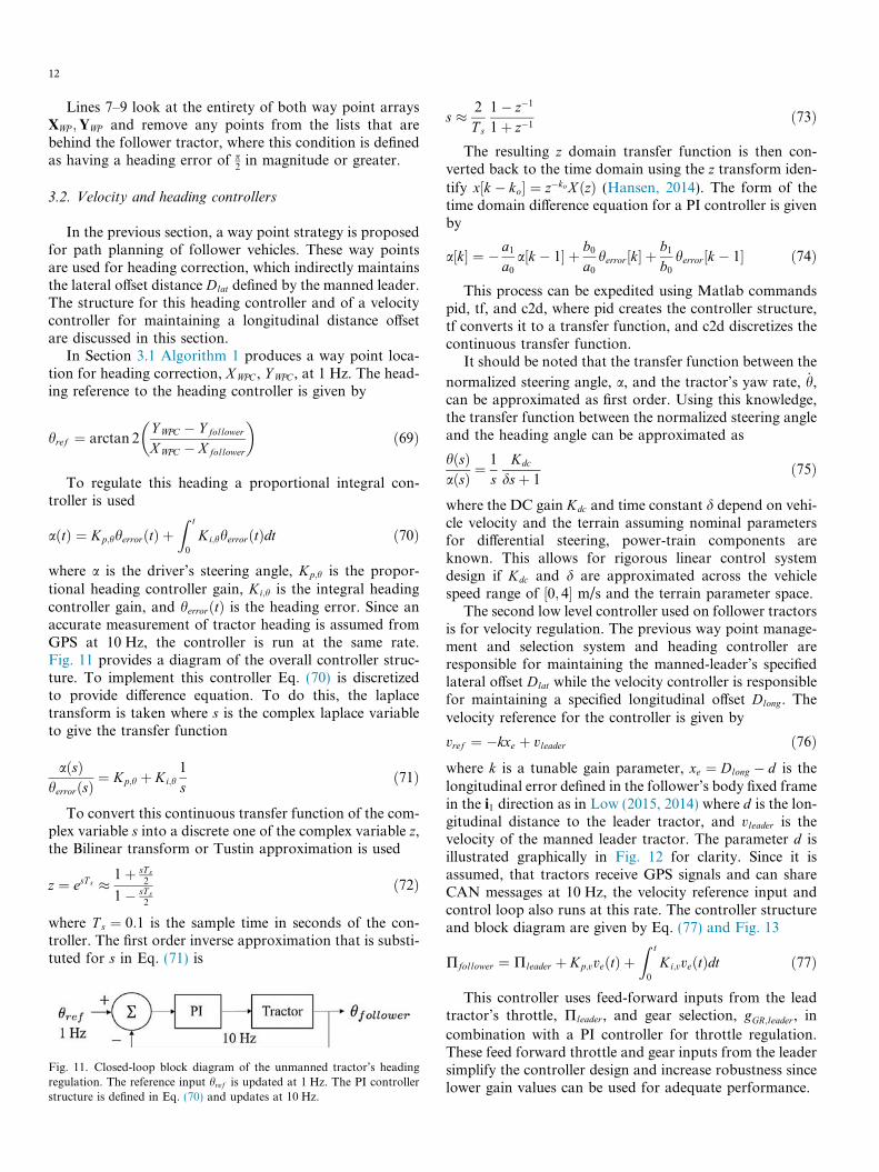
The second low level controller used on follower tractorsis for velocity regulation. The previous way point manage-ment and selection system and heading controller areresponsible for maintaining the manned-leader’s specifiedlateral offset Dlat while the velocity controller is responsiblefor maintaining a specified longitudinal offset Dlong. Thevelocity reference for the controller is given by

vref ¼ �kxe þ vleader ð76Þwhere k is a tunable gain parameter, xe ¼ Dlong � d is thelongitudinal error defined in the follower’s body fixed framein the i1 direction as in Low (2015, 2014) where d is the lon-gitudinal distance to the leader tractor, and vleader is thevelocity of the manned leader tractor. The parameter d isillustrated graphically in Fig. 12 for clarity. Since it isassumed, that tractors receive GPS signals and can shareCAN messages at 10 Hz, the velocity reference input andcontrol loop also runs at this rate. The controller structureand block diagram are given by Eq. (77) and Fig. 13

Pfollower ¼ Pleader þ Kp;vveðtÞ þZ t

0

Ki;vveðtÞdt ð77Þ

This controller uses feed-forward inputs from the leadtractor’s throttle, Pleader, and gear selection, gGR;leader, in

combination with a PI controller for throttle regulation.These feed forward throttle and gear inputs from the leadersimplify the controller design and increase robustness sincelower gain values can be used for adequate performance.

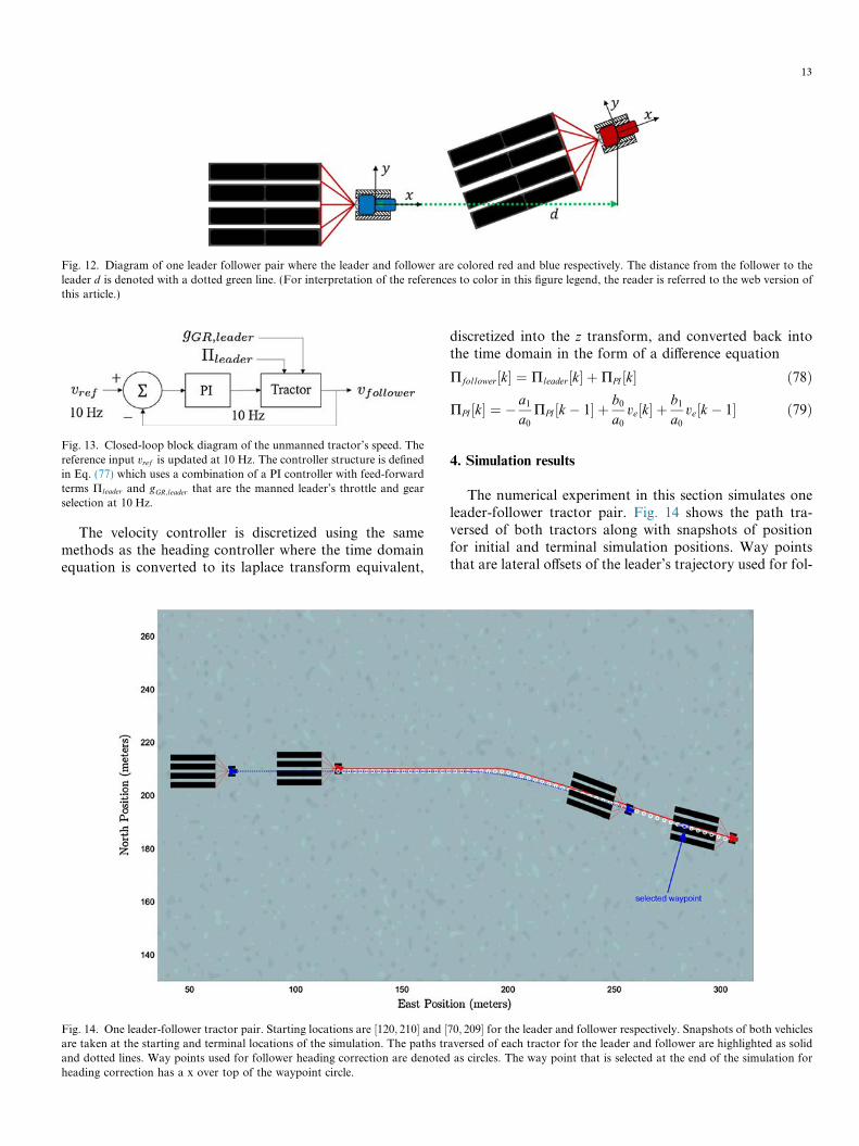
Fig. 13. Closed-loop block diagram of the unmanned tractor’s speed. Thereference input vref is updated at 10 Hz. The controller structure is definedin Eq. (77) which uses a combination of a PI controller with feed-forwardterms Pleader and gGR;leader that are the manned leader’s throttle and gearselection at 10 Hz.

Fig. 12. Diagram of one leader follower pair where the leader and follower are colored red and blue respectively. The distance from the follower to theleader d is denoted with a dotted green line. (For interpretation of the references to color in this figure legend, the reader is referred to the web version ofthis article.)

13

The velocity controller is discretized using the samemethods as the heading controller where the time domainequation is converted to its laplace transform equivalent,

Fig. 14. One leader-follower tractor pair. Starting locations are ½120; 210� and ½are taken at the starting and terminal locations of the simulation. The paths trand dotted lines. Way points used for follower heading correction are denotedheading correction has a x over top of the waypoint circle.

discretized into the z transform, and converted back intothe time domain in the form of a difference equation

Pfollower½k� ¼ Pleader½k� þPPI ½k� ð78Þ

PPI ½k� ¼ � a1a0

PPI ½k � 1� þ b0a0

ve½k� þ b1a0

ve½k � 1� ð79Þ

4. Simulation results

The numerical experiment in this section simulates oneleader-follower tractor pair. Fig. 14 shows the path tra-versed of both tractors along with snapshots of positionfor initial and terminal simulation positions. Way pointsthat are lateral offsets of the leader’s trajectory used for fol-

70; 209� for the leader and follower respectively. Snapshots of both vehiclesaversed of each tractor for the leader and follower are highlighted as solidas circles. The way point that is selected at the end of the simulation for

14

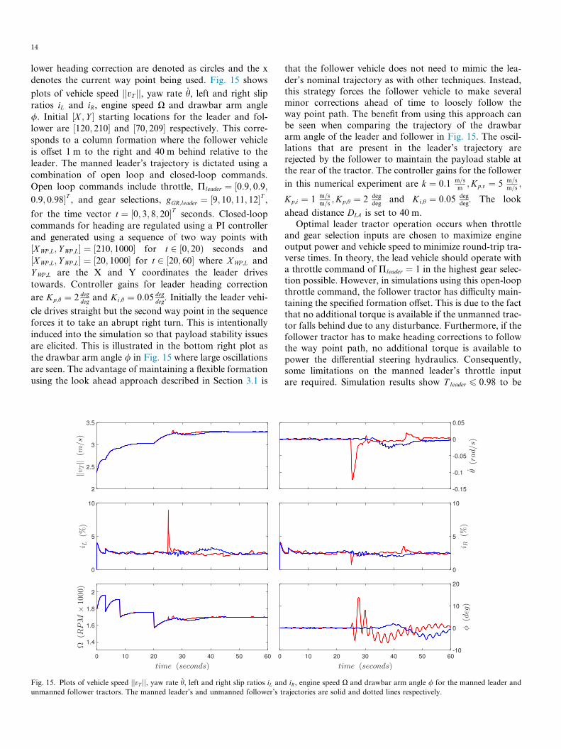
lower heading correction are denoted as circles and the xdenotes the current way point being used. Fig. 15 shows

plots of vehicle speed jjvT jj, yaw rate _h, left and right slipratios iL and iR, engine speed X and drawbar arm angle/. Initial ½X ; Y � starting locations for the leader and fol-lower are ½120; 210� and ½70; 209� respectively. This corre-sponds to a column formation where the follower vehicleis offset 1 m to the right and 40 m behind relative to theleader. The manned leader’s trajectory is dictated using acombination of open loop and closed-loop commands.Open loop commands include throttle, Pleader ¼ ½0:9; 0:9;0:9; 0:98�T , and gear selections, gGR;leader ¼ ½9; 10; 11; 12�T ,for the time vector t ¼ ½0; 3; 8; 20�T seconds. Closed-loopcommands for heading are regulated using a PI controllerand generated using a sequence of two way points with½XWP ;L; Y WP ;L� ¼ ½210; 1000� for t 2 ½0; 20Þ seconds and½XWP ;L; Y WP ;L� ¼ ½20; 1000� for t 2 ½20; 60� where XWP ;L andY WP ;L are the X and Y coordinates the leader drivestowards. Controller gains for leader heading correction

are Kp;h ¼ 2 deg

degand Ki;h ¼ 0:05 deg

deg. Initially the leader vehi-

cle drives straight but the second way point in the sequenceforces it to take an abrupt right turn. This is intentionallyinduced into the simulation so that payload stability issuesare elicited. This is illustrated in the bottom right plot asthe drawbar arm angle / in Fig. 15 where large oscillationsare seen. The advantage of maintaining a flexible formationusing the look ahead approach described in Section 3.1 is

Fig. 15. Plots of vehicle speed jjvT jj, yaw rate _h, left and right slip ratios iL anunmanned follower tractors. The manned leader’s and unmanned follower’s t

that the follower vehicle does not need to mimic the lea-der’s nominal trajectory as with other techniques. Instead,this strategy forces the follower vehicle to make severalminor corrections ahead of time to loosely follow theway point path. The benefit from using this approach canbe seen when comparing the trajectory of the drawbararm angle of the leader and follower in Fig. 15. The oscil-lations that are present in the leader’s trajectory arerejected by the follower to maintain the payload stable atthe rear of the tractor. The controller gains for the follower

in this numerical experiment are k ¼ 0:1 m=sm;Kp;v ¼ 5 m=s

m=s;

Kp;i ¼ 1 m=sm=s

;Kp;h ¼ 2 degdeg

and Ki;h ¼ 0:05 degdeg. The look

ahead distance DLA is set to 40 m.Optimal leader tractor operation occurs when throttle

and gear selection inputs are chosen to maximize engineoutput power and vehicle speed to minimize round-trip tra-verse times. In theory, the lead vehicle should operate witha throttle command of Pleader ¼ 1 in the highest gear selec-tion possible. However, in simulations using this open-loopthrottle command, the follower tractor has difficulty main-taining the specified formation offset. This is due to the factthat no additional torque is available if the unmanned trac-tor falls behind due to any disturbance. Furthermore, if thefollower tractor has to make heading corrections to followthe way point path, no additional torque is available topower the differential steering hydraulics. Consequently,some limitations on the manned leader’s throttle inputare required. Simulation results show T leader 6 0:98 to be

d iR, engine speed X and drawbar arm angle / for the manned leader andrajectories are solid and dotted lines respectively.

15

sufficient. The effect of an additional load from the differen-tial steering hydraulics can be seen when looking at plots ofengine speed in Fig. 15 between 30 and 40 s where bothvehicles see a reduction in engine RPM.

5. Conclusion

A comprehensive tracked vehicle dynamics model hasbeen developed including the effects of the powertrain,terrain-vehicle interaction, and payload on deformable ter-rain with relatively low computational cost. This can beused as a powerful tool for fast, iterative model-baseddesign to test autonomous tractor algorithms and tune con-trollers across different operating conditions and expectedterrains.

In this paper, a partially autonomous tractor system isproposed with a human in the loop specifically taking theform a manned leader, autonomous follower vehicle pair.Emphasis is placed on maintaining a flexible formationso that the unmanned vehicle has the capability to rejecthuman error in driving. This is done using a combinationof way points as a path guide along with a look-ahead tech-nique. Simulation results show the effectiveness of thisapproach: when a manned leader takes an abrupt turnand experiences large drawbar oscillations, the unmannedfollower keeps its payload stable.

Future work for implementation will investigate theexpected, discrete terrain parameter space to approximatelinear plant dynamics for heading correction across differ-ent vehicle speeds as discussed in Section 3.2. Then con-trollers can be designed using linear system techniques.Other work could include developing an adaptive look-ahead distance for unmanned vehicles based on the trailerstability of the manned leader. This way, follower vehiclesdo not need to deviate from the way point path by anunnecessary amount.

Acknowledgement

This work was supported by NASA grantNNX-10AL97H.

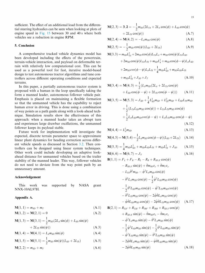
Appendix A.

Mð1; 1Þ ¼ mSD þ mT ðA:1ÞMð1; 2Þ ¼ Mð2; 1Þ ¼ 0 ðA:2Þ

Mð1; 3Þ ¼ Mð3; 1Þ ¼ 1

2mSDð2LA sinð/Þ þ LSD sinðwÞ

þ 2LTS sinðwÞÞ ðA:3ÞMð1; 4Þ ¼ Mð4; 1Þ ¼ LAmSD sinð/Þ ðA:4Þ

Mð1; 5Þ ¼ Mð5; 1Þ ¼ 1

2mSD sinðwÞðLSD þ 2LTSÞ ðA:5Þ

Mð2; 2Þ ¼ mSD þ mT ðA:6Þ

Mð2; 3Þ ¼ 3; 2 ¼ � 1

2mSDð2LTA þ 2LA cosð/Þ þ LSD cosðwÞ

þ 2LTS cosðwÞÞ ðA:7ÞMð2; 4Þ ¼ Mð4; 2Þ ¼ �LAmSD cosð/Þ ðA:8Þ

Mð2; 5Þ ¼ � 1

2mSD cosðwÞðLSD þ 2LTSÞ ðA:9Þ

Mð3;3Þ¼mSDL2TAþ2mSD cosð/ÞLTALAþmSD cosðwÞLTALSD

þ2mSD cosðwÞLTALTS þmSDL2AþmSD cosð/�wÞLALSD

þ2mSDcosð/�wÞLALTS þ1

4mSDL2

SDþmSDLSDLTS

þmSDL2TS þ JSDþ JT ðA:10Þ

Mð3; 4Þ ¼ Mð4; 3Þ ¼ 1

2ðLAmSDð2LA þ 2LTA cosð/Þ

þ LSD cosð/� wÞ þ 2LTS cosð/� wÞÞÞ ðA:11Þ

Mð3; 5Þ ¼ Mð5; 3Þ ¼ JSD þ 1

4L2SDmSD þ L2

TSmSD þ LSDLTSmSD

þ 1

2ðLTALSDmSD cosðwÞÞ þ LTALTSmSD cosðwÞ

þ 1

2LALSDmSDcosð/� wÞ þ LALTSmSD cosð/� wÞ

ðA:12ÞMð4; 4Þ ¼ L2

AmSD ðA:13Þ

Mð4;5Þ¼Mð5;4Þ¼ 1

2LAmSD cosð/�wÞðLSDþ2LTSÞ ðA:14Þ

Mð5; 5Þ ¼ 1

4mSDL2

SD þ mSDLSDLTS þ mSDL2TS þ JSD ðA:15Þ

Mð6; 6Þ ¼ Mð6; 7Þ ¼ JS ðA:16ÞBð1; 1Þ ¼ F L þ F R � RL � RR þ RSD;X cosðwÞ

� RSD;Y sinðwÞ þ _hmSDvy þ _hmT vy

� LTA_h2mSD � _/2LAmSD cosð/Þ

� _h2LAmSD cosð/Þ � 1

2_w2LSDmSD cosðwÞ

� 1

2_h2LSDmSD cosðwÞ � _w2LTSmSDcosðwÞ

� _h2LTSmSD cosðwÞ � 2 _/ _hLAmSD cosð/Þ� _w _hLSDmSD cosðwÞ � 2 _w _hLTSmSD cosðwÞ ðA:17Þ

Bð2; 1Þ ¼ RlLF þ RlLR þ RlRF þ RlRR þ RSD;Y cosðwÞþ RSD;X sinðwÞ � _hmSDvx � _hmT vx

� _/2LAmSD sinð/Þ � _h2LAmSD sinð/Þ

� 1

2_w2LSDmSD sinðwÞ � 1

2_h2LSDmSD sinðwÞ

� _w2LTSmSD sinðwÞ � _h2LTSmSD sinðwÞ� 2 _/ _hLAmSD sinð/Þ � _w _hLSDmSD sinðwÞ� 2 _w _hLTSmSD sinðwÞ ðA:18Þ

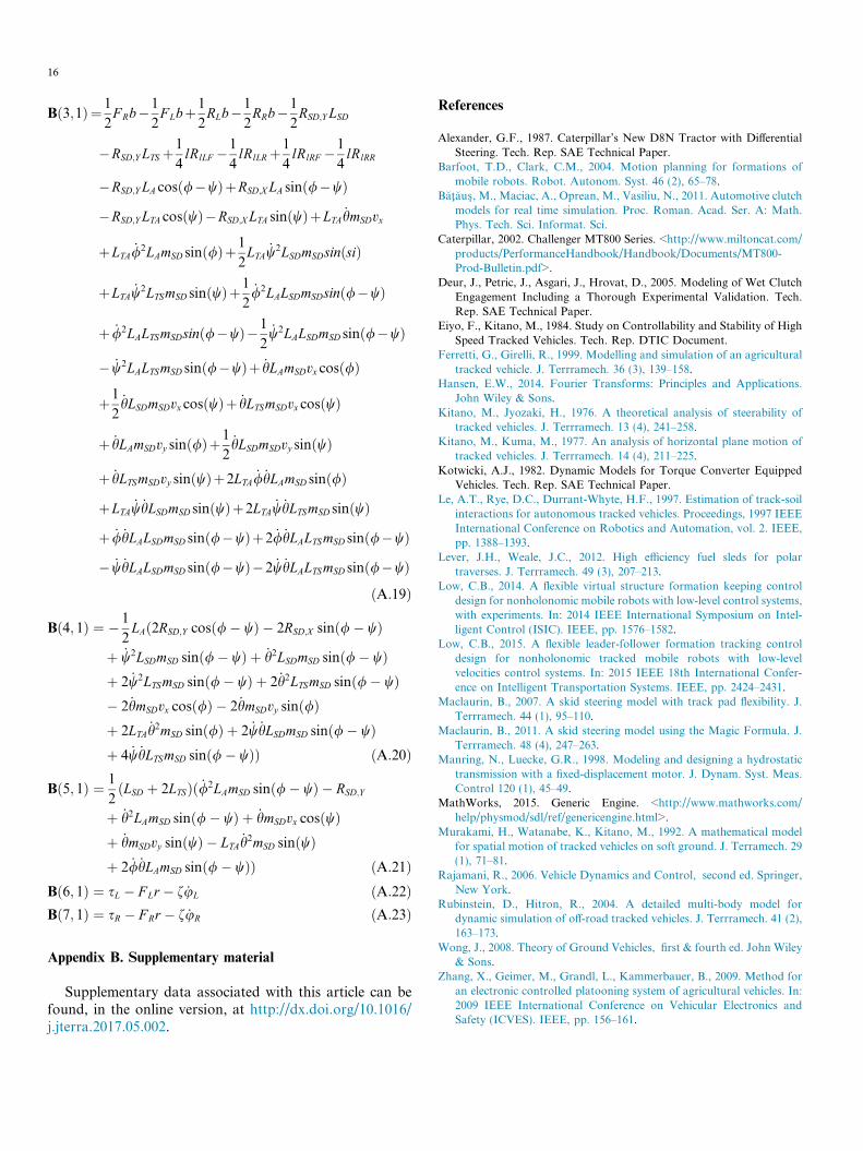
16

Bð3;1Þ¼ 1

2F Rb�1

2F Lbþ1

2RLb�1

2RRb�1

2RSD;Y LSD

�RSD;Y LTS þ1

4lRlLF �1

4lRlLRþ1

4lRlRF �1

4lRlRR

�RSD;Y LA cosð/�wÞþRSD;XLA sinð/�wÞ�RSD;Y LTA cosðwÞ�RSD;XLTA sinðwÞþLTA

_hmSDvx

þLTA_/2LAmSD sinð/Þþ1

2LTA

_w2LSDmSDsinðsiÞ

þLTA_w2LTSmSD sinðwÞþ1

2_/2LALSDmSDsinð/�wÞ

þ _/2LALTSmSDsinð/�wÞ�1

2_w2LALSDmSD sinð/�wÞ

� _w2LALTSmSD sinð/�wÞþ _hLAmSDvx cosð/Þ

þ1

2_hLSDmSDvx cosðwÞþ _hLTSmSDvx cosðwÞ

þ _hLAmSDvy sinð/Þþ1

2_hLSDmSDvy sinðwÞ

þ _hLTSmSDvy sinðwÞþ2LTA_/ _hLAmSD sinð/Þ

þLTA_w _hLSDmSD sinðwÞþ2LTA

_w _hLTSmSD sinðwÞþ _/ _hLALSDmSD sinð/�wÞþ2 _/ _hLALTSmSD sinð/�wÞ� _w _hLALSDmSD sinð/�wÞ�2 _w _hLALTSmSD sinð/�wÞ

ðA:19Þ

Bð4; 1Þ ¼ � 1

2LAð2RSD;Y cosð/� wÞ � 2RSD;X sinð/� wÞ

þ _w2LSDmSD sinð/� wÞ þ _h2LSDmSD sinð/� wÞþ 2 _w2LTSmSD sinð/� wÞ þ 2 _h2LTSmSD sinð/� wÞ� 2 _hmSDvx cosð/Þ � 2 _hmSDvy sinð/Þþ 2LTA

_h2mSD sinð/Þ þ 2 _w _hLSDmSD sinð/� wÞþ 4 _w _hLTSmSD sinð/� wÞÞ ðA:20Þ

Bð5; 1Þ ¼ 1

2ðLSD þ 2LTSÞð _/2LAmSD sinð/� wÞ � RSD;Y

þ _h2LAmSD sinð/� wÞ þ _hmSDvx cosðwÞþ _hmSDvy sinðwÞ � LTA

_h2mSD sinðwÞþ 2 _/ _hLAmSD sinð/� wÞÞ ðA:21Þ

Bð6; 1Þ ¼ sL � F Lr � f _uL ðA:22ÞBð7; 1Þ ¼ sR � F Rr � f _uR ðA:23Þ

Appendix B. Supplementary material

Supplementary data associated with this article can befound, in the online version, at http://dx.doi.org/10.1016/j.jterra.2017.05.002.

References

Alexander, G.F., 1987. Caterpillar’s New D8N Tractor with DifferentialSteering. Tech. Rep. SAE Technical Paper.

Barfoot, T.D., Clark, C.M., 2004. Motion planning for formations ofmobile robots. Robot. Autonom. Syst. 46 (2), 65–78.

Bataus�, M., Maciac, A., Oprean, M., Vasiliu, N., 2011. Automotive clutchmodels for real time simulation. Proc. Roman. Acad. Ser. A: Math.Phys. Tech. Sci. Informat. Sci.

Caterpillar, 2002. Challenger MT800 Series. <http://www.miltoncat.com/products/PerformanceHandbook/Handbook/Documents/MT800-Prod-Bulletin.pdf>.

Deur, J., Petric, J., Asgari, J., Hrovat, D., 2005. Modeling of Wet ClutchEngagement Including a Thorough Experimental Validation. Tech.Rep. SAE Technical Paper.

Eiyo, F., Kitano, M., 1984. Study on Controllability and Stability of HighSpeed Tracked Vehicles. Tech. Rep. DTIC Document.

Ferretti, G., Girelli, R., 1999. Modelling and simulation of an agriculturaltracked vehicle. J. Terrramech. 36 (3), 139–158.

Hansen, E.W., 2014. Fourier Transforms: Principles and Applications.John Wiley & Sons.

Kitano, M., Jyozaki, H., 1976. A theoretical analysis of steerability oftracked vehicles. J. Terrramech. 13 (4), 241–258.

Kitano, M., Kuma, M., 1977. An analysis of horizontal plane motion oftracked vehicles. J. Terrramech. 14 (4), 211–225.

Kotwicki, A.J., 1982. Dynamic Models for Torque Converter EquippedVehicles. Tech. Rep. SAE Technical Paper.

Le, A.T., Rye, D.C., Durrant-Whyte, H.F., 1997. Estimation of track-soilinteractions for autonomous tracked vehicles. Proceedings, 1997 IEEEInternational Conference on Robotics and Automation, vol. 2. IEEE,pp. 1388–1393.

Lever, J.H., Weale, J.C., 2012. High efficiency fuel sleds for polartraverses. J. Terrramech. 49 (3), 207–213.

Low, C.B., 2014. A flexible virtual structure formation keeping controldesign for nonholonomic mobile robots with low-level control systems,with experiments. In: 2014 IEEE International Symposium on Intel-ligent Control (ISIC). IEEE, pp. 1576–1582.

Low, C.B., 2015. A flexible leader-follower formation tracking controldesign for nonholonomic tracked mobile robots with low-levelvelocities control systems. In: 2015 IEEE 18th International Confer-ence on Intelligent Transportation Systems. IEEE, pp. 2424–2431.

Maclaurin, B., 2007. A skid steering model with track pad flexibility. J.Terrramech. 44 (1), 95–110.

Maclaurin, B., 2011. A skid steering model using the Magic Formula. J.Terrramech. 48 (4), 247–263.

Manring, N., Luecke, G.R., 1998. Modeling and designing a hydrostatictransmission with a fixed-displacement motor. J. Dynam. Syst. Meas.Control 120 (1), 45–49.

MathWorks, 2015. Generic Engine. <http://www.mathworks.com/help/physmod/sdl/ref/genericengine.html>.

Murakami, H., Watanabe, K., Kitano, M., 1992. A mathematical modelfor spatial motion of tracked vehicles on soft ground. J. Terramech. 29(1), 71–81.

Rajamani, R., 2006. Vehicle Dynamics and Control, second ed. Springer,New York.

Rubinstein, D., Hitron, R., 2004. A detailed multi-body model fordynamic simulation of off-road tracked vehicles. J. Terrramech. 41 (2),163–173.

Wong, J., 2008. Theory of Ground Vehicles, first & fourth ed. John Wiley& Sons.

Zhang, X., Geimer, M., Grandl, L., Kammerbauer, B., 2009. Method foran electronic controlled platooning system of agricultural vehicles. In:2009 IEEE International Conference on Vehicular Electronics andSafety (ICVES). IEEE, pp. 156–161.

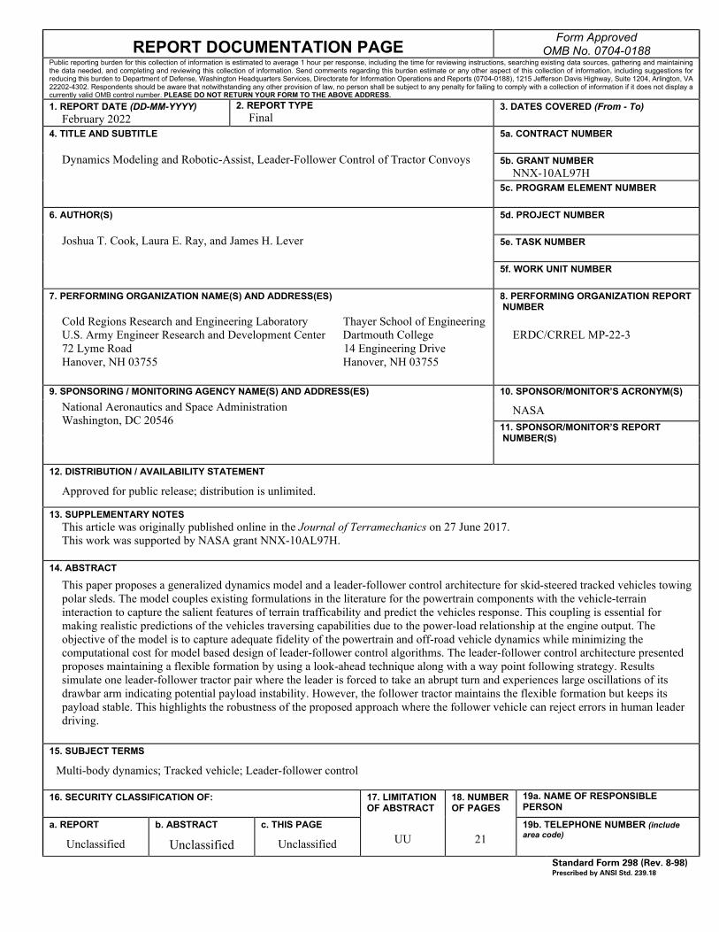
REPORT DOCUMENTATION PAGE Form Approved OMB No. 0704-0188

Public reporting burden for this collection of information is estimated to average 1 hour per response, including the time for reviewing instructions, searching existing data sources, gathering and maintaining the data needed, and completing and reviewing this collection of information. Send comments regarding this burden estimate or any other aspect of this collection of information, including suggestions for reducing this burden to Department of Defense, Washington Headquarters Services, Directorate for Information Operations and Reports (0704-0188), 1215 Jefferson Davis Highway, Suite 1204, Arlington, VA 22202-4302. Respondents should be aware that notwithstanding any other provision of law, no person shall be subject to any penalty for failing to comply with a collection of information if it does not display a currently valid OMB control number. PLEASE DO NOT RETURN YOUR FORM TO THE ABOVE ADDRESS. 1. REPORT DATE (DD-MM-YYYY)

February 2022 2. REPORT TYPE

Final 3. DATES COVERED (From - To)

4. TITLE AND SUBTITLE

Dynamics Modeling and Robotic-Assist, Leader-Follower Control of Tractor Convoys

5a. CONTRACT NUMBER

5b. GRANT NUMBER NNX-10AL97H

5c. PROGRAM ELEMENT NUMBER

6. AUTHOR(S) Joshua T. Cook, Laura E. Ray, and James H. Lever

5d. PROJECT NUMBER

5e. TASK NUMBER

5f. WORK UNIT NUMBER

7. PERFORMING ORGANIZATION NAME(S) AND ADDRESS(ES) 8. PERFORMING ORGANIZATION REPORT NUMBER

Cold Regions Research and Engineering Laboratory Thayer School of Engineering U.S. Army Engineer Research and Development Center Dartmouth College 72 Lyme Road 14 Engineering Drive Hanover, NH 03755 Hanover, NH 03755

ERDC/CRREL MP-22-3

9. SPONSORING / MONITORING AGENCY NAME(S) AND ADDRESS(ES) 10. SPONSOR/MONITOR’S ACRONYM(S) National Aeronautics and Space Administration Washington, DC 20546

NASA 11. SPONSOR/MONITOR’S REPORT NUMBER(S)

12. DISTRIBUTION / AVAILABILITY STATEMENT

Approved for public release; distribution is unlimited.

13. SUPPLEMENTARY NOTES This article was originally published online in the Journal of Terramechanics on 27 June 2017. This work was supported by NASA grant NNX-10AL97H.

14. ABSTRACT

This paper proposes a generalized dynamics model and a leader-follower control architecture for skid-steered tracked vehicles towing polar sleds. The model couples existing formulations in the literature for the powertrain components with the vehicle-terrain interaction to capture the salient features of terrain trafficability and predict the vehicles response. This coupling is essential for making realistic predictions of the vehicles traversing capabilities due to the power-load relationship at the engine output. The objective of the model is to capture adequate fidelity of the powertrain and off-road vehicle dynamics while minimizing the computational cost for model based design of leader-follower control algorithms. The leader-follower control architecture presented proposes maintaining a flexible formation by using a look-ahead technique along with a way point following strategy. Results simulate one leader-follower tractor pair where the leader is forced to take an abrupt turn and experiences large oscillations of its drawbar arm indicating potential payload instability. However, the follower tractor maintains the flexible formation but keeps its payload stable. This highlights the robustness of the proposed approach where the follower vehicle can reject errors in human leader driving.

15. SUBJECT TERMS

Multi-body dynamics; Tracked vehicle; Leader-follower control

16. SECURITY CLASSIFICATION OF: 17. LIMITATION OF ABSTRACT

18. NUMBER OF PAGES

19a. NAME OF RESPONSIBLE PERSON

a. REPORT

Unclassified

b. ABSTRACT

Unclassified c. THIS PAGE

Unclassified UU 21 19b. TELEPHONE NUMBER (include area code)

Standard Form 298 (Rev. 8-98) Prescribed by ANSI Std. 239.18