Embed Size (px)
Citation preview

Kent Academic RepositoryFull text document (pdf)
Copyright & reuseContent in the Kent Academic Repository is made available for research purposes. Unless otherwise stated allcontent is protected by copyright and in the absence of an open licence (eg Creative Commons), permissions for further reuse of content should be sought from the publisher, author or other copyright holder.
Versions of researchThe version in the Kent Academic Repository may differ from the final published version. Users are advised to check http://kar.kent.ac.uk for the status of the paper. Users should always cite the published version of record.
EnquiriesFor any further enquiries regarding the licence status of this document, please contact: [email protected]
If you believe this document infringes copyright then please contact the KAR admin team with the take-down information provided at http://kar.kent.ac.uk/contact.html
Citation for published version
Mitchell, Simon Leo (2019) Novel approaches to inform tropical bird conservation in humanmodified landscapes. Doctor of Philosophy (PhD) thesis, University of Kent,.
DOI
Link to record in KAR
https://kar.kent.ac.uk/76185/
Document Version
UNSPECIFIED
Novel approaches to inform tropical bird
conservation in human modified landscapes
Simon Leo Mitchell
Durrell Institute of Conservation and Ecology
School of Anthropology and Conservation
University of Kent | Canterbury | Kent
Thesis submitted for the degree of Doctor of Philosophy in
Biodiversity Management
February 2019
Word count: 50,654
Bornean Blue Flycatcher, Simon Mitchell

i
Dedicated to my Dad, Roger Mitchell whose enthusiasm for birds and wildlife started me on this path.
And to my mum, Marysia Dubeck who has offered unwavering support for everything I do.
(Don’t worry guys, this doesn’t mean you have to read this whole thing!)

ii
Acknowledgements
My first thanks must go to my supervisors. Matt Struebig has been an incredible
academic mentor for the last four year, guiding me through the intricacies of everything from
Malaysian immigration, to reviewer comments! I consider myself very lucky to have him as
a supervisor and friend. Zoe Davies has offered not only amazingly detailed feedback,
thoughtful suggestions and enthusiastic support, but also emotional support at the most
challenging times. The general narrative regarding academia seems to be that it’s highly
competitive, stressful and cutthroat. However, Matt and Zoe, as well as the rest of the DICE
family, have always made it something collaborative, challenging and actually exciting and I
sincerely look forward to the possibility of working with them further in future. Huge thanks
also to Dave Edwards, for initially suggesting I apply for the PhD position, providing excellent
feedback and overall support throughout, and of course opening my eyes to tropical avifauna
and ornthiological science to begin with!
Long fieldwork seasons are often a slog, but I feel mine were enhanced immeasurably
by the wonderful company of Ryan Grey, Josh Twining, Adeline Seah, Craig Brelsford,
Christina Murray, Rosie Drinkwater, Mike Massam, Tor Kemp, Mike Boyle, Joe Williamson,
Jess Hightower, Dave Hemrich-Bennet, Jess Haysom, Adam Sharp, Zosia Ladds, Cindy Eva
Cosset, Luke Nelson. My fieldwork in Sabah would not have been possible without the
amazing SAFE team. Thanks to Jamiluddin “Unding” Jami for coordinating field logistics.
Thanks also to all the excellent field assistants: Arnold “Noy” James, Mohd. “Kiky” Shah
Nizam Bin Mustamin, Ampat “Anis” Siliwong and Najmuddin “Mudin” Jamal and Sabidee
“Didy” Mohd. Rizan.
Many other people were also kind enough to contribute as collaborators, offer helpful
pointers or taught me particular techniques or statistical approaches. These include Tom
Swinfield, David Milodowski, Joe Tobias, Alex Lees, James Eaton, Marina Jiminez, Alex

iii
Greene, Ross Crates, Eleni Matechou. Special thanks go James Gilroy for giving up his time
so generously to teach me two solid days of occupancy modelling techniques!
So many people have made DICE a really great place to be. Foremost amongst are
Gwili Gibbon, who has always been there when I need someone to vent to, and Nick Deere
who has dropped everything to provide me with help, statistical assistance and a drinking
buddy on countless occasions! Even though our PhD have no thematic overlap whatsoever,
Nick’s sharp mind has motivated me to achieve more than I thought possible. I’d also like to
extend my gratitude and appreciation to Jess Fisher, Kate Alberry, Alistair Key, Dave Seaman,
Jake Bicknell, Gui Braga Ferreira, (Isa)Bela Menezes-Barata, Valeria Boron, Tristan Pett and
Lydia Tiller, Simon Tollington, Bob Smith, James Kloda and anyone else I may have failed
to mention specifically by name.
Through the trials and tribulations of the last four years also I’d like to thank my old
friends Mike Hoit, Keith Langdon, Teegan Dochery, Jacob Best, Jack Stewart, Stephen Hall,
Stephen Wagstaff, Tea Basic, Igor Ormus, Helena Nery Alves Pinto, Sara Minarro for their
support. Extra special thanks go to Alice Milton, for sticking by me throughout and
brightening everything from mist-shrouded rainforests to dismal British winters with her
wonderful wit, support and companionship.
Last but not least I would like to thank my brother and sister, and especially my
parents. To my dad for creating and nurtuing my passion for the natural world championing
my every endeavour and to my mum for always being there to support me in everything.

iv
Author’s declaration
The contents of this thesis were written by Simon L. Mitchell with the incorportation
of suggestions, feedback and editorial ammendments made by Matthew J. Struebig and Zoe
G. Zavies. Associated dataset and code will be made available through NERC EDR and other
online repositories at the time of chapter publications.
Chapter 1: SLM wrote the chapter. Comments and feedback were provided by MJS.
Chapter 2: SLM, MJS, DPE, HB and ZGD conceived and designed the methodology;
SLM collected, processed and analysed bird encounter data; DC and TJ processed LiDAR
data; SLM, led the writing of the manuscript. All authors contributed critically to the drafts
and gave final approval for publication. This chapter was published in the Journal of Applied
Ecology.
Chapter 3: SLM conceived the idea undertook all fieldwork. Data analysis was
undertaken by SLM, with suggestions from MJS, ZGD, NJD and JG. DC, TS, DM and TJ
processed LiDAR data and provided specific measures for each site. SLM produced the
figures and wrote the Chapter, with feedback and comments from MJS, ZGD and DPE. NDJ
provided comments on the occupancy modelling description incorporated in the methods.
Chapter 4: SLM conceived the idea undertook all fieldwork. Data analysis was
undertaken by SLM, with suggestions from MJS and ZGD. SLM produced the figures and
wrote the Chapter, with feedback and comments from MJS, ZGD and DPE.
Chapter 5: SLM wrote the chapter. Comments and feedback were provided by MJS.
I hereby declare that there were no competing interests on behalf of all co-authors.

v
Abstract
In this thesis I utilise a combination of newly advanced methodological and
statistical approaches to assess knowledge gaps concerning biodiversity in human-
modified tropical landscapes. Specifically, I use cutting-edge LiDAR technology,
occupancy modelling and soundscape analysis to document the responses of tropical birds
to land-use change in Borneo.
I first evaluate the contribution that riparian reserves – protected natural vegetation
around waterways in production landscapes – have in supporting biodiversity. By
assessing the avian community structure and richness of riparian reserves I demonstrate
that these landscape features can offer significant biodiversity benefits, and support
comparable levels of species diversity to logged riparian forests provided they are of
sufficient size (>80 m in total width) and habitat quality (>75 tC ha-1 of tree biomass). I
show that in oil palm estates riparian reserves would need to be >200 m in total width (i.e.
100 m from each riverbank) to preserve comparable numbers of forest specialist bird to
logged riparian forest.
I then examine whether responses of species and trait groups to habitat disruption
follow linear trajectories or non-linear responses whereby abrupt changes to occupancy
and diversity occur once thresholds of disturbance are exceeded. Habitat disruption across
a land-cover gradient from intact forest to oil palm plantations was characterised via
LiDAR metrics that quantify habitat structure in three dimensions. By scrutinising the
individual responses of 171 bird species and 17 different multi-species trait groups to these
metrics via hierarchical multi-species occupancy modelling, I show that the majority of
species respond to habitat degradation in a non-linear fashion. I demonstrate that
thresholds in species response scale up to abrupt changes in trait group richness,
particularly those associated with important ecosystem functions such as pollination, seed

vi
dispersal and insectivory. I find trait groups exhibit highly varied thresholds from one
another. I also highlight how exceeding particular thresholds of degradation in human
modified tropical landscapes could result in abrupt changes to ecosystem functioning,
thereby making human-modified tropical landscape less resilient to further perturbations.
Last, I seek to test the application of recently developed acoustic approaches for
monitoring biodiversity in human-modified tropical landscapes. I assess the performance
of five commonly used ‘soundscape’ indices in corresponding to variation in observed or
estimated bird diversity from field data. I find that sources of acoustic bias in production
landscapes (including human produced noise and the sound of running), make broad
application of acoustic monitoring technologies to heavily disturbed habitats such as
intensive farmland challenging. I demonstrate that controlling for time-of-day, using
noise-reduction algorithms and excluding certain habitat types, improves the capacity of
acoustic indices to reflect both observed bird richness, and estimates of species numbers
derived from occupancy models.
Taken together, the three studies in this thesis reveal the biodiversity value of
riparian areas, the potential for non-linear responses of species to habitat change, and the
efficacy of novel monitoring techniques applied to biodiversity monitoring in human-
modified tropical landscapes. I offer a number of recommendations and applications of
these three sets of findings and explore their implication for biodiversity conservation in
tropical regions. By addressing these three knowledge gaps using a combination of newly
available innovations I demonstrate not only the importance of the findings themselves,
but also highlight how innovations in technology, analytical technique and monitoring
approach when used in conjunction can elucidate biodiversity patterns that were otherwise
less well known.

vii
Acknowledgements ................................................................................................ ii
Author’s declaration ............................................................................................. iv
Abstract……………………………………………………………………………...v
List of tables ........................................................................................................... x
List of supplementary tables................................................................................. xi
List of figures ....................................................................................................... xii
List of supplementary figures ............................................................................. xiii
Introduction ....................................................................................... 1
A global environmental and biodiversity crisis........................................ 1
The degradation and destruction of tropical forests, and implications for
biodiversity……….. ................................................................................. 2
Forest degradation in the context of Southeast Asia’s biodiversity crisis 5
Biodiversity in human-modified tropical landscapes .............................. 6
Birds as biodiversity indicators ............................................................. 10
Survey and monitoring challenges for birds ......................................... 11
Thesis structure ..................................................................................... 16
References ............................................................................................ 18
Riparian reserves help protect forest bird communities in oil palm
dominated landscapes...................................................................... 32
Abstract ........................................................................................................ 33
Introduction .................................................................................................. 34
Methods ........................................................................................................ 37
Study system .......................................................................................... 37
Bird sampling ........................................................................................ 39
Environmental predictors of bird community structure ........................ 40
Statistical analyses ................................................................................ 41
Results.. ........................................................................................................ 44
Species abundance and richness ........................................................... 44
Bird community composition ................................................................ 48
Environmental predictors of riparian reserve communities .................. 49
Discussion .................................................................................................... 53
Management recommendations ............................................................ 57

viii
Supplemental Materials................................................................................. 59
Acknowledgements ....................................................................................... 63
References .................................................................................................... 63
Species traits predict thresholds of nonlinear response to forest
change .............................................................................................. 70
Abstract ........................................................................................................ 71
Introduction .................................................................................................. 72
Materials and methods .................................................................................. 76
Study system .......................................................................................... 76
Bird sampling ........................................................................................ 78
LiDAR-based forest structure and configuration predictors ................. 79
Occupancy modelling ............................................................................ 80
Species trait groups ............................................................................... 84
Deriving group-level richness from occupancy models ......................... 85
Results.. ........................................................................................................ 85
Effect sizes of occupancy responses to forest cover and structure......... 85
Group richness effects and thresholds .................................................. 86
Species thresholds ................................................................................. 94
Discussion .................................................................................................... 95
Pervasive non-linear responses to habitat change in the tropical bird
community…. ........................................................................................ 96
Patterns in trait-group responses to forest disturbance ......................... 97
Idiosyncratic species responses ............................................................. 99
Detecting species responses in narrow ranges of environmental
change……… ..................................................................................... 100
Implications for biodiversity assessment, forest management and
conservation planning.................................................................................. 101
Supplementary information ......................................................................... 104
Ackowledgements....................................................................................... 134
References .................................................................................................. 134
Sound methods for monitoring tropical biodiversity: Optimising
acoustic indices to reflect species richness in forest habitats ....... 147
Abstract ...................................................................................................... 148
Introduction ................................................................................................ 149
Methods ...................................................................................................... 152
Bird sampling ...................................................................................... 152

ix
Acoustic Indices .................................................................................. 154
Estimated species richness .................................................................. 157
LiDAR forest metrics........................................................................... 157
Statistical analyses .............................................................................. 158
Results… .................................................................................................... 160
Assocations between acoustic indices and point count richness.......... 160
Effects of habitat type .......................................................................... 163
Effects of noise-reduction processing ................................................. 165
Assocations between time-controlled indices, estimated richness and
canopy height ............................................................................................... 166
Discussion .................................................................................................. 168
Supplemental Materials............................................................................... 177
Acknowledgements ..................................................................................... 180
References .................................................................................................. 180
Discussion ...................................................................................... 191
The application of LiDAR technologies in biodiversity monitoring .... 191
Challenges in occupancy modelling to monitor rare species ............... 194
The application of bioacoustic approaches to biodiversity monitoring 197
Synergies between novel approaches and technologies ....................... 200
References .................................................................................................. 203
Appendix: Co-authored publications: ............................................................. 209
Riparian buffers in tropical agriculture: Scientific support, effectiveness and
directions for policy ......................................................................... 209
Co-producing knowledge for environmental sustainability: defining the .... 210

x
List of tables
Table 2.1. Outputs of generalised linear models (GLM) and generalised linear mixed
effects models (GLMM)…………………………………………………………….50
Table 3.1. Threshold levels in trait group richness. ................................................. 86
Table 4.1. Linear regression model statistics of observed bird richness and time-of-
day ....................................................................................................................... 161
Table 4.2. General linear models for each acoustic index in relation to richness, time-
of-day, and habitat types covariates. ..................................................................... 163
xi
List of supplementary tables
Table S 2.1. Sampling dates and mean intervals for each site. ................................ 60
Table S 2.2. Indicator species for each of four different habitat types. .................... 62
Table S 3.1. Vegetation strata associations, feeding guilds and habitat associations of
the birds of lowland Sabah. .................................................................................. 104
Table S 3.2. Details of feeding guild and habitat association codes used in the study.
............................................................................................................................ 109
Table S 3.3. Median thresholds points with confidence intervals in relation to mean
canopy height and canopy hereogeneity. .............................................................. 110
Table S 3.4. Median thresholds points with confidence intervals in relation to density
height and skew. .................................................................................................. 115
Table S 3.5. Median thresholds points with confidence intervals in relation to density
height and skew. .................................................................................................. 120
Table S 3.6. Results of Kruskall Wallis tests for differences in group average effects
and threshold levels between trait groups ............................................................. 132

xii
List of figures
Figure 2.1 Map of the Stability of Altered Forest Ecosystems (SAFE) Landscape. . 38
Figure 2.2. Boxplots of site-level bird abundance and species richness. .................. 45
Figure 2.3. Nonmetric multidimensional scaling ordinations of bird community
structure. ................................................................................................................ 47
Figure 2.4. Observed species richness for riparian reserves and oil palm river sites 49
Figure 3.1. Map of Sabah showing four study landscapes. ...................................... 78
Figure 3.2. Species richness predicted by the segmented models for strata associations.
.............................................................................................................................. 89
Figure 3.3. Species group richness predicted by the best segmented models for nine
avian feeding guilds. .............................................................................................. 90
Figure 3.4. Segmented models for different species of the arboreal frugivore feeding
guild. ..................................................................................................................... 91
Figure 3.5. Segmented model for different species within the arboreal gleaning
insectivores / frugivores guilds. .............................................................................. 93
Figure 4.1. Relationships between acoustic indices and observed avian richness .. 162
Figure 5.2. Time-controlled versions of the three best performing indices in predicting
estimated richness of birds and canopy height…………………………………………..

xiii
List of supplementary figures
Figure S 2.1. Rarefied bird species accumulation curves for each riparian and control
habitat .................................................................................................................... 59
Figure S 3.1. Occupancy-modelled species-level effects of mean canopy height within
50 m radius. ......................................................................................................... 125
Figure S 3.2. Occupancy-modelled species-level effects of canopy heterogeneity with
50 m radius. ......................................................................................................... 126
Figure S 3.3. Occupancy-modelled species-level effects of mean vegetation density
within 50 m radius. .............................................................................................. 127
Figure S 3.4. Occupancy-modelled species-level effects of mean vegetation skew
within 50 m radius. .............................................................................................. 128
Figure S 3.5. Occupancy-modelled species-level effects of forest cover within 100 m
radius. .................................................................................................................. 129
Figure S 3.6. Boxplots showing the distribution of threshold levels for different strata
assocations, feeding guilds and habitat assocations .............................................. 130
Figure S 4.1. Violin plots with embedded boxplots for adjusted indices. .............. 177
Figure S 4.2. Regressions of the best performing indices against observed species
richness. ............................................................................................................... 178

1
Introduction
A global environmental and biodiversity crisis
Anthropological degradation of the biosphere continues unabated, with
societies continuing to operate beyond the planetary boundaries required to sustain
human civilisation (Butler, 2017), 35% of non-human species (Thomas et al., 2004)
and potentially human life (Stern Review, U.K Treasury, 2007). Currently,
biodiversity loss, climate forcing and nitrogen pollution all exceed what is deemed the
‘safe operating space for humanity’ (Rockström et al., 2009), with levels of ocean
acidification and phosphorus pollution also approaching these boundaries (Carpenter
& Bennett, 2011; Kawaguchi et al., 2013) The scale of effects on the biosphere are
now so pervasive that there is growing concern the planet could become almost
uninhabitable to humans in a few generations (Barnosky et al., 2012), especially when
overall patterns of resource use and degradation are accelerating (Steffen, Broadgate,
Deutsch, Gaffney, & Ludwig, 2015). Increasingly, civil unrest and war (Kelley et al.,
2015), famine (Barnett & Adger, 2007) and the rise of authoritarianism (Steinhardt &
Wu, 2015) are being driven in part, by societal responses to environmental
degradation.
Of the planetary boundaries currently being exceeded, biodiversity loss is
occurring at levels furthest beyond those considered ‘safe’ (Rockström et al., 2009).
Rates of vertebrate extinction during the last hundred years are at least ~100 times
those of the background rate of extinction, suggesting a six major extinction event is
already underway (Ceballos et al., 2015). It is estimated that the amount of genetic

2
diversity already lost would take over 200,000 human generations to be regained
through evolutionary processes (Myers, 1993). This unprecedented pace of
biodiversity loss (Pimm et al., 1995), is eroding the capacity of natural ecosystems to
provide goods and services which benefit human wellbeing (Diaz et al., 2006).
Biodiversity underpins the fundamental characteristics of ecosystems, and
species losses can compromise ecosystem function and resilience to external
perturbations (Cardinale et al., 2006). Species losses worldwide are already having
comparable effects upon primary productivity to other forms of environmental change
(Hooper et al., 2012). Since 1500 there have been 338 documented vertebrate
extinctions (Young et al., 2016). However, the majority of historic and prehistoric
extinctions caused by humans probably went unnoticed. Modelled estimates suggest
that close to 1000 species of non-passerine land bird went extinct in the Pacific region
alone (Duncan et al., 2013). It is projected that a further 130,000 species could become
extinct across all taxa by 2060 (Pimm & Raven, 2000). The accelerating crises in
biodiversity loss specifically, and environmental degradation more generally, make
directing effective and prescient conservation interventions to the most important
regions and habitats of the world all the more important.
The degradation and destruction of tropical forests, and implications for biodiversity
Biodiversity is patchily distributed across the planet and highly concentrated
in the tropics, where around two-thirds of all life on earth occurs, particularly in humid
rainforests (Pimm & Raven, 2000). The tropics in general are hyperdiverse and
account for 90% of terrestrial bird species, virtually all shallow-water corals, and over

3
75% of known amphibians, freshwater fish, ant, terrestrial mammals and flowering
plants (Barlow et al., 2018). Within tropical regions forests are the most diverse
habitats, with about half of the world’s known taxa occurring (Scheffers et al., 2012).
The distribution of these forests largely mirror 25 biodiversity hotspots, where around
30-50% of plant, amphibian, reptile and bird species occur (Pimm & Raven, 2000).
However, these same regions have some of the highest human population densities
and growth rates globally (Cincotta, et al., 2000), as well as the most rapid rates of
landuse change (Jantz et al., 2015). Since 1990, around five million hectares of
tropical forest have been lost per year (Keenan et al., 2015). Landuse change in the
tropics has been the single greatest driver of biodiversity loss (Baille et al., 2004).
Remote sensing analyses reveal 80% of the world’s tropical forests to already
be somewhat degraded (Potapov et al., 2017). Conservation scientists have argued
that, in this context, primary forest conservation is paramount, since it is irreplaceable
for biodiversity (Gibson et al., 2011). Undisturbed forests may be especially important
in the context of climate change, given the thermal buffering capacity of forests is
compromised by edge effects (Ewers & Banks-Leite, 2013). However, intact tropical
forests continue to be cleared at an accelerating rate, with the global extent reduced by
8.4% between 2000 and 2013 (Potapov et al., 2017).
Drivers of deforestation and forest degradation vary in terms of their relative
importance globally, but 70% of overall forest loss is attributable to direct human land
use conversion (Song et al., 2018) and agriculture is the strongest driver of tropical
forest loss globally (Gibbs et al., 2010). Commercial agriculture is a stronger driver
than subsistence farming, whilst mining operations, infrastructural expansion and
urban development also contribute significantly (Hosonuma et al., 2012). Human

4
populations are predicted to continue to expand to around 9-11 billion people by 2050
(Vörösmarty et al., 2000) and a 70-100% increase in agricultural production is
expected to be necessary in order to satisfy the additional population as well as
increases in consumption (Tilman et al., 2001; Godfray et al., 2010). Projections
estimate natural vegetative cover in biodiversity hotspots will be reduced by a further
26-58% by 2100, precipitating hundreds or thousands of extinctions in tetrapods alone
(Jantz et al., 2015).
In the last decade, the value of degraded tropical forests for biodiversity
conservation has become more widely recognised. In part, this is an enforced
pragmatic approach on the part of conservation scientists, since the proportion of
primary forest is declining, and the alternative to retaining degraded forest is often
more intensive agricultural landuse (Lindenmayer & Franklin, 2002; Meijaard &
Sheil, 2007). However, the proportion of species from primary forests that persist in
heavily logged areas is often substantial, even if those species persist at reduced
abundances. Whilst the levels of species numbers retained are highly taxon and region
specific (Gibson et al., 2011), for twelve out of fifteen taxonomic groups assessed in
Amazonia more than half the species found in primary forest persisted in logged forest
areas (Barlow, et al., 2007). In Borneo, studies have also concluded that >75% of bird
and dung beetle species from unlogged forest are still present within forest logged
multiple times (Edwards et al., 2010). Similarly, research on insectivorous bats
showed no definitive effect of logging on site-level richness (Struebig et al., 2013).
Additional justifications for the conservation and restoration of logged and degraded
forests have been offered in terms of the provision of ecosystem services (Chazdon,
2008), including carbon sequestration (Chazdon et al., 2016).

5
Forest degradation in the context of Southeast Asia’s biodiversity crisis
Sodhi first highlighted the biodiversity crisis in Southeast Asia in 2004 (Sodhi
et al., 2004). The Southeast Asia region has perhaps the greatest degree of endemism
of anywhere in the world (Kier et al., 2009). Both current and projected rates of forest
loss are higher here than for the global average in the tropics (Laurance, 2007), and
the extent of lowland primary forest is vanishingly small. The yield and value of timber
in Southeast Asia is higher than anywhere else in the world, resulting in major
incentives for the unsustainable logging. In Borneo, in particular, the value of timber
extracted between 1980 and 2000 was greater than that of tropical Africa and Latin
America combined (Curran et al., 2004), and around 1.6% of forest is lost per year
(Wilcove et al., 2013). Modelled estimates suggest that 7-52% of lowland forest bird
species and 9-36% of lowland forest mammals are likely to go extinct under business
as usual logging scenarios (Wilcove et al., 2013). Biodiversity loss in the region is
also compounded by high hunting pressures (Harrison et al., 2016) due in part to
geographic proximity to Chinese markets, where demand for rare species causes an
‘anthropic allee’ for several Southeast Asian taxa (Courchamp et al., 2006). Uniquely
for the tropics many bird species are also in high demand, either as pet songbirds or
for use in traditional medicine (Nijman, et al., 2018). Southeast Asia is currently one
of the regions with most taxa on the IUCN Red List, with 3,319 species listed as
Vulnerable, Endangered or Critically Endangered, including 318 species of birds
(IUCN, 2018).
In recent years, the expansion of oil palm (Elaeis guineensis) agriculture has
been one of the leading drivers of deforestation in Southeast Asia. Oil palm is among
the most profitable production land uses in the tropics and now covers an estimated

6
18.7 million ha globally (Meijaard et al., 2018). At least 522 Mha of tropical forest
was converted to oil palm between 1980 and 2000 (Gibbs et al., 2010) and an
additional 150 Mha was cleared between 2000 and 2012 (Hansen et al. 2013). In
Kalimantan, Indonesian Borneo, 90% of oil palm expansion from 1990 to 2010
replaced some type of forest; (47% intact forest, 22% logged forest, and 21%
agroforest) (Carlson et al., 2012). Demand is expected to continue to increase with a
growing global population and affluence (Sayer et al., 2012). Expansion to meet this
demand could extend the oil palm footprint to 800,000 ha of forest in Colombia by
2020 (Garcia-Ulloa et al., 2012), and more than 6.5 million ha by 2080 on Borneo
(Struebig et al., 2015). Since the climatic niche for cultivating oil palm is similar to
that of tropical forests (Pirker et al., 2016), oil palm expansion is also likely to continue
in other hyper-diverse ecoregions. Therefore, understanding the extent to which
biodiversity can be preserved within oil-palm landscapes and how best to manage the
competing demands of oil palm production and conservation efforts to maximise both
biodiversity protection and human wellbeing is of paramount importance.
Biodiversity in human-modified tropical landscapes
Given that over 40% of the earth’s terrestrial land surface is currently under
agricultural management (Perfecto & Vandermeer, 2010), and virtually all tropical
habitats are either managed or exploited by people (Kareiva et al., 2007) there has
been increasing research focus on biodiversity in rural landscapes which undergo
active management or modification by people (Gardner et al., 2009). Since a mere
10% of tropical forests are formally protected (Schmitt et al., 2009), the capacity of
reserves to provide adequate protection to tropical fauna and flora is strongly

7
influenced by anthropogenic activities in adjacent land (Wittemyer et al. 2008). On
this basis, it is argued that conservation science needs to adopt a systematic approach
which incorporates the socio-ecological interplay between rural human populations
and protected lands in order to offer more holistic solution to problems of biodiversity
conservation (Liu et al. 2007).
In human-modified tropical landscapes any remaining forest is typically
limited to remnants surrounded by agriculture, with such patches comprising native
vegetation, secondary regrowth and pioneer vegetation (Laurance et al., 2014). The
status of biodiversity in these landscapes, and the factors that most affect it, remain
poorly understood (Chazdon et al., 2009), but a combination of the spatial extent and
configuration of remnant natural vegetation are thought to be the main drivers of
biodiversity patterns (Ewers, & Didham, 2006), as well as both the intensity of landuse
(Tscharntke et al., 2012) and the structural and ecological characteristics of crop
species (Phalan, 2011). Recent research has highlighted that such landscapes,
particularly those that occur along a gradient between undisturbed tropical forest and
agriculture, may have comparable levels of alpha (i.e. within site) and beta (i.e.
between site) diversity to undisturbed habitats, but distinctly lower levels of gamma
(i.e. landscape) diversity (de Castro Solar et al., 2015). Biodiversity is thought to be
critically important for the maintenance and resilience of ecosystem function in these
systems (Lohbeck et al., 2016).
The patchwork nature of human-modified tropical forests means research on
the responses of biodiversity to fragmentation is highly relevant to understanding these
systems fully. However, when trying to address ecological questions over human-
modified tropical landscapes holistically, the idea of isolated habitat patches located

8
in an inhospitable matrix may represent an incomplete way of understanding the
system. Fragmentation models assume that there is a clear contrast between human-
defined patches and the rest of the landscape and that multiple organisms perceive this
as suitable habitat, which may not always be the case in landscapes where agriculture
or extraction is of low intensity or fragments are also highly degraded (Fischer &
Lindenmayer, 2006). The amount and structure of native vegetation, prevalence of
anthropogenic edges, degree of landscape connectivity and structure and heterogeneity
of modified areas all affect species assemblages in fragmented systems (Fischer &
Lindenmeyer, 2007) and these can be useful properties to consider in human-modified
landscapes more generally. It is still relevant that the highest levels of biodiversity in
agricultural landscapes tend to be in the largest remnant fragments (Heegaard et al.,
2007) with the greatest degree of structural similarity to continuous undisturbed
forests (Decaëns et al., 2018), since even landscape-wide conservation interventions
should necessarily prioritise the preservation of the areas with the highest levels of
richness alongside other management approaches adopted.
Land-sparing and sharing frameworks are also useful when considering the
overall efficacy of different approaches to protect biodiversity in human-modified
tropical landscapes. Land-sparing approaches focus on attempts to maintain refuges
for biodiversity separate from croplands (Fischer et al., 2008; Edwards et al., 2010;
Phalan, 2011), whilst land sharing focuses on employing wildlife-friendly farming
methods to enhance (or preserve) biodiversity on productive lands (Clough et al.,
2011; Pywell et al., 2012). The trade-off between two the approaches appears to be
mediated by regional context and crop type as land-sparing is fairly successful in
preserving biodiversity in coffee and cacao dominated landscapes (Gobbi, et al., 2000;

9
Clough et al., 2001), but generally less successful in oil palm areas (Edwards et al.,
2010). The success of land-sharing may also be affected by the type and proximity of
surrounding habitats (Gilroy et al., 2014).
Oil palm plantations typically support very low levels of biodiversity. Large
reductions in diversity are reported for birds (Edwards et al., 2010); bats in forest
(Danielsen & Heergaard, 1995); mammals (Scott et al., 2004) beetles (Chung et al.,
2000) and ants (Brul 2001). Among 25 studies comparing biodiversity between logged
forest and oil palm, 23 found significant negative effects (Savilaasko et al., 2014).
However, the majority of these studies focussed strictly upon plantation areas. When
considered as whole landscapes, oil palm estates frequently include remnant forest
fragments of varying size. These areas are known to support considerable biodiversity
from studies of forest birds (Edwards et al., 2010), bats (Struebig et al., 2008) and ants
(Bruhl et al., 2003), for example. A recent multi-taxa synthesis suggested that
fragments in oil palm landscapes need to be a minimum of 200 ha in size in order to
maintain a ‘minimum viable core’ area (defined as supporting at least 60% of species
found in continuous forest) (Lucey et al., 2017). The landscape-scale differences
between industrial and smallholder oil palm agriculture remain uncertain, although the
latter appears to have a lower overall negative effect on birds (Azhar et al., 2011).
Understanding the landscape-wide potential for biodiversity conservation in
oil palm estates requires ecological valuation of native forests retained not only in
‘conventional’ fragments, but also in riparian forest remnants. In many oil palm
landscapes, riparian forest remnants comprise the majority of natural vegetation (pers.
obs.), meaning their contribution to landscape-wide patterns of biodiversity in oil palm
landscapes is potentially considerable. Whilst riparian reserves may in some ways be

10
considered in the framework of fragmentation as long, linear fragments, the ecology
of riparian forests is somewhat distinct from that of non-riparian forest. For example,
some taxa are riparian or non-riparian specialists and occur as obligates in their
respective habitats (Naiman et al, 1998) and the resulting community overlaps with
that of the surrounding landscape in terms of species composition, but also contains
unique species. The biodiversity value for riparian forest remnants in oil palm
landscapes has already been demonstrated for dung beetles, ants (Gray, 2014) and fish
(Giam et al., 2015), but remains poorly assessed for other taxa.
Birds as biodiversity indicators
Globally, patterns of avian biodiversity mirror those of other taxa, with the
greatest biodiversity in the tropics (Jetz, 2012). Global threats facing the birds are also
well understood. Of a global estimate of ~10,000 species 1,492 are currently listed as
vulnerable, endangered or critically endangered (IUCN, 2018).
Landuse change is the most significant threat to birds around the world. Even
in scenarios that assume no additional affects from climate change, at least 400 of
8750 modelled species are projected to experience >50% range reductions by the year
2050 (Jetz et al., 2007). The Red List Index for birds, (which provides an indexed
metric of the changing levels of endangerment of extinction) showed a 7% worsening
in the status of the world birds between 1988 and 2004 (Butchart et al., 2004).
Disaggregated indices showed deteriorations across all major ecosystems, but the
steepest declines occurred in the indices for Sundaic birds (i.e. those found in the

11
Malay peninsula, Sumatra, Java and Borneo), which were driven by intensifying
destruction of lowland forests (Butchart et al., 2004).
Birds exhibit many of the features required of biodiversity indicators: they are
diverse (Jetz et al., 2012); respond to multiple environmental changes in similar
patterns to the majority of other taxa; and can be surveyed more cost-effectively than
many other taxa (Gardner et al., 2008). Birds (alongside mammals) are also the
world’s best-studied taxonomic group (Costello, 2015), which means new research
findings are often more easily contextualised in terms of their broader significance
than might be the case for other taxa. However, accurately surveying tropical bird
communities is often more difficult than generally appreciated by researchers who do
not specialise in these taxa (Robinson et al., 2018). The challenge of accurately
identifying and counting birds in typically dark, structurally complex rainforest
environments where upwards of 95% of species are only encountered aurally, is often
underestimated (Robinson et al., 2018). Many species have varied acoustic repertoires
including multiple short vocalisations, which can lead to difficulty in avoiding false
negative detections by non-experts (Robinson et al., 2018). The utility of studies with
systematic false-negative detections can potentially be compromised (Remsen, 1994).
Survey and monitoring challenges for birds
In the context of the challenges highlighted above, the monitoring and
assessment of both temporal and spatial patterns of biodiversity generally, and bird
diversity specifically, is increasingly important in conservation. Without adequate
monitoring and assessment efforts, predictions of impending species declines,
12
extinctions, and subsequent recommendations for intervention are compromised. Nor
is it possible to reliably assess the effectiveness of management practices or
conservation efforts without appropriate data for evaluating those practices
(Lindenmayer et al., 2010). Monitoring biodiversity also provides a potential first
warning for the collapse of associated ecosystems, which underpin societal well-being
(Rowland et al., 2018; Scholes et al. 2008). The Aichi Biodiversity Targets specify
goals such as “improving the status of biodiversity by safeguarding ecosystems,
species and genetic diversity.” Evaluations to date show that these global targets have
so far been largely missed (Tittensor et al., 2014). Implementing new conservation
efforts to meet them, necessarily involves biodiversity monitors. Given the available
funding for biodiversity conservation globally is insufficient to meet all conservation
needs (McCarthy et al., 2012), using the most effective methods of monitoring and
assessing biodiversity is highly important (Balmford et al., 2000). Monitoring efforts
should also yield data that are accurate and as ecologically relevant as possible, in
order to detect the effects of often cryptic stressors or patterns, which may have
profound effects when upscaling study outcomes across large spatial or temporal
scales.
In the last 20 years a significant number of innovations have increased our
capacity to monitor and assess the responses and patterns of biodiversity in relation to
environmental variation in tropical forests, as well as improve the efficiency and cost
of monitoring efforts (Pimm et al., 2015). Broadly, these fall into categories of new
methods and means of capturing biodiversity data, new methods of assessing and
measuring environmental variation, and improved analytical approaches for
comparing and integrating biodiversity and environmental data. New methods of

13
characterizing biodiversity include autonomous camera traps and acoustic recorders
(Steenweg et al., 2017) while environmental DNA monitoring is moving from lab-
based to field-based assessment techniques (Thomsen & Willerslev, 2015).
One example of a novel technological approach to biodiversity which has
resulted in significant increases in efficiency in capturing species data is that of
autonomous acoustic monitoring techniques. These techniques have only become
feasible recently on large scales through the reduced cost of recording technology (Hill
et al., 2018). Soundscape ecology covers a number of techniques that focus on
analysing the interaction of organisms, environmental drivers and human impacts
based on their associated acoustic properties (Gasc et al., 2013). Such approaches
allow the assessment and monitoring of biodiversity in a highly passive manner, with
potentially little need for human expertise or effort once autonomous acoustic sensors
can be set up.
The means to capture environmental data affecting biodiversity also advanced
very rapidly over the last two decades. Freely-available remote sensed datasets were
limited to Landsat satellite imagery at the turn of the century (Nagendra, 2001; Wang,
et al., 2010). As well as vastly improvement in fine-grain resolution of existing
technologies the addition of Synthetic Aperture Radar (SAR) and aerial Light
Detection And Ranging (LiDAR) allows the ability to assess structural aspects of
vegetation. Advances in drone technology, combined with the algorithms and
computing power now also make forest canopy mapping in three dimensions possible
via photogrammetry (Saarinen et al., 2017).
Perhaps the most notable single advance comes from hyper-spectral LiDAR,
which provides the ability to map the fine-scale structure of vegetation in three

14
dimensions and thereby offers the potential to analyse patterns of faunal distribution
and association which were previously unachievable. In tropical forests assessing
vegetation in three dimensions is especially relevant, since vertical components in
these landscapes are inherently important, with up to 70% of species utilising the upper
forest strata on a facultative basis (Kays & Allison, 1975). Vertical dimensions are
even more important for taxa such as birds and flying insects, and communities often
change markedly from terrestrial-feeders to arboreal specialists (Chmel et al., 2016;
Stork et al., 2015). LiDAR-based studies have addressed the effects of habitat extent,
canopy height, canopy heterogeneity, vertical canopy distribution, understory density,
aspect, elevation, slope and ruggedness have described responses in taxa as diverse as
birds, mammals, insects and fish (Davies, et al., 2014).
Novel analytical approaches include a vast range of techniques such as
improvements in accounting for specific challenges such as imperfect species
detection (Jennelle, Runge, & MacKenzie, 2002), advances in meta-analytic
approaches to determine effects across multiple systems (Pardo et al., 2013), rapid
advances in GIS and spatial statistical approaches such as the development of MaxEnt
for distribution modelling (Elith et al., 2011), the application of deep learning
computing techniques in analysing ever larger datasets such as those collected through
citizen science (Kelling et al., 2013), or to deal with advances in population genetics
via environmental DNA (Cordier et al., 2017) or classify remote sensed data (Hethcoat
et al., 2018). Other techniques which have been refined and/or adopted more widely
include new ways of conceptualising biotic communities, from approaches such as
functional diversity (Cadotte, Carscadden, & Mirotchnick, 2011), to phylogenic

15
diversity (Tucker et al., 2017) and the analyses of potential thresholds in species and
community responses (Ficetola & Denoe, 2009).
One innovation which could potentially facilitate the detection of far more
cryptic responses of species and communities is the increase in data power and error
estimation associated with occupancy modelling. Virtually all methods of biodiversity
surveying suffer from imperfect detection and complete species surveys are often
unfeasible (Iknayan et al. 2014). Traditional rarefaction methods have focused on
measures which account for the difficulty in detecting rare species by offering the
means to assess when communities have been adequately sampled (Chao & Jost,
2012), and extrapolating species accumulation curves to estimate metrics such as
species richness and community Hill numbers (Palmer, 1990; Chao et al., 2014).
Occupancy modelling uses repeat sampling to estimate the probability of false
negative detections and then controls for these in overall models (Jennelle, 2002).
Concerns have been raised that in some cases gearing study design toward these
analyses may result in focusing finite survey effort inefficiently or inappropriately.
This is because the amount of data required to obtain ‘naïve’ estimates is generally
substantially lower than that required for estimates which adjust for imperfect
detection, when in fact, improved study design can surmount problems of imperfect
detection (Banks-Leite et al., 2014). Other authors have suggested that although good
survey design is fundamental, it will not necessarily solve all detection problems or
control for all variation in detectability (Guillera-Aroita, 2017).

16
Thesis structure
In this thesis I integrate the use of recent advances in biodiversity monitoring
in order to address practical knowledge gaps relevant to conservation management in
human-modified tropical landscapes. I combine multiple novel approaches to assess
the relative biodiversity value of different habitats and provide management
recommendations to optimise biodiversity provision in a tropical production
landscape, elucidate hitherto unrecognised ecological patterns and refine novel
analytical approaches themselves. I focus on Southeast Asia throughout, with a
specific research focus in the lowlands of Eastern Sabah, Malaysian Borneo.
In Chapter 1, I examine the species diversity present in riparian reserves
compared to riparian forest controls. I also determine the proportion of forest-
specialist species remaining in these reserves. I use LiDAR derived remote-sensing
data to measure the widths and carbon densities of riparian reserves within oil palm
estates. Using these data I estimate the optimal riparian reserve widths and carbon
densities necessary to support a similar level of species richness to riparian forest
controls in continuous forests.
I use Chapter 2 to focus on the ecological patterns exhibited by the avifaunal
community along a continuous gradient of forest degradation using a trait-based
approach. I combine a Bayesian occupancy model, parameterised with LiDAR-
derived vegetation structure data, with piece-wise regression analyses to assess
thresholds in both species and trait group responses to habitat change. Using this
approach I infer likely species response thresholds to multiple environmental variables
and am able to elaborate on the way particular trait groups have previously been

17
observed to respond to changes in forest structure by identifying points of abrupt
change in these responses.
In Chapter 3 I seek to improve the application of soundscape analysis to
biodiversity monitoring by offering recommendations to optimise how well acoustic
indices reflect bird communities as measured by conventional point count approaches
and species richness as defined by the occupancy model described in Chapter 2. By
assessing the influence of controlling for time-of-day and background noise in
recordings, and removing habitats where certain indices are non-functional, I am able
to offer recommendations as to which indices are most robust for assessing
biodiversity in human modified tropical landscapes.
In the Introduction and Discussion sections of this thesis I have adopted a first
person singular style. However, given the collaborative nature of the data chapter, I
switch to a combination first person plural or passive voice throughout these sections.

18
References
Azhar, B., Lindenmayer, D. B., Wood, J., Fischer, J., Manning, A., McElhinny, C., &
Zakaria, M. (2011). The conservation value of oil palm plantation estates,
smallholdings and logged peat swamp forest for birds. Forest Ecology and
Management, 262(12), 2306–2315.
Baillie, J., Hilton-Taylor, C., & Stuart, S. N. (Eds.). (2004). 2004 IUCN red list of
threatened species: a global species assessment. IUCN
Balmford, A., Gaston, K. J., Rodrigues, A. S., & James, A. (2000). Integrating Costs of
Conservation into International Priority Setting. Conservation Biology, 14(3), 597-
605.
Banks-Leite, C., Pardini, R., Boscolo, D., Cassano, C. R., Püttker, T., Barros, C. S., &
Barlow, J. (2014). Assessing the utility of statistical adjustments for imperfect
detection in tropical conservation science. Journal of Applied Ecology, 51(4), 849–
859.
Barlow, J., França, F., Gardner, T. A., Hicks, C. C., Lennox, G. D., Berenguer, E., …
Graham, N. A. J. (2018). The future of hyperdiverse tropical ecosystems. Nature,
559(7715).
Barlow, J., Mestre, L. A. M., Gardner, T. A., & Peres, C. A. (2007). The value of primary,
secondary and plantation forests for Amazonian birds. Biological Conservation,
136(2), 212–231.
Barnett, J., & Adger, W. N. (2007). Climate change, human security and violent conflict.
Political Geography, 26(6), 639–655.
Barnosky, A. D., Hadly, E. A., Bascompte, J., Berlow, E. L., Brown, J. H., Fortelius, M.,
… Smith, A. B. (2012). Approaching a state shift in Earth’s biosphere. Nature,
486(7401), 52–58.
Brühl, C. A. 2001. Leaf litter ant communities in tropical lowland rain forests in Sabah,
Malaysia: effects of forest disturbance and fragmentation. Thesis. University of
Würzburg, Würzburg , Germany

19
Butchart, S. H. M., Stattersfield, A. J., Bennun, L. A., Shutes, S. M., Akçakaya, H. R.,
Baillie, J. E. M., … Mace, G. M. (2004). Measuring global trends in the status of
biodiversity: Red list indices for birds. PLoS Biology, 2(12).
Butler,C. D. (2017). Limits to growth, planetary boundaries, and planetary health. Current
Opinion in Environmental Sustainability, 25, 59-65.
Cadotte, M. W., Carscadden, K., & Mirotchnick, N. (2011). Beyond species: Functional
diversity and the maintenance of ecological processes and services. Journal of Applied
Ecology, 48(5), 1079–1087.
Cardinale, B. J., Srivastava, D. S., Duffy, J. E., Wright, J. P., Downing, A. L., Sankaran,
M., & Jouseau, C. (2006). Effects of biodiversity on the functioning of trophic groups
and ecosystems. Nature, 443(7114), 989.
Carlson, K. M., Curran, L. M., Ratnasari, D., Pittman, A. M., Soares-Filho, B. S., Asner,
G. P., ... & Rodrigues, H. O. (2012). Committed carbon emissions, deforestation, and
community land conversion from oil palm plantation expansion in West Kalimantan,
Indonesia. Proceedings of the National Academy of Sciences, 109(19), 7559-7564.
Carpenter, S. R., & Bennett, E. M. (2011). Reconsideration of the planetary boundary for
phosphorus. Environmental Research Letters, 6(1).
Ceballos, G., García, A., Pringle, R. M., Ceballos, G., Ehrlich, P. R., Barnosky, A. D., …
Palmer, T. M. (2015). Accelerated modern human – induced species losses : Entering
the sixth mass extinction. Science Advances, 1(June), 1–6.
Chao, A., & Jost, L. (2012). Coverage-based rarefaction and extrapolation: Standardizing
samples by completeness rather than size. Ecology, 93(12), 2533–2547.
Chao, A., Gotelli, N. J., Hsieh, T. C., Sander, E. L., Ma, K. H., Colwell, R. K., & Ellison,
A. M. (2014). Rarefaction and extrapolation with Hill numbers: A framework for
sampling and estimation in species diversity studies. Ecological Monographs, 84(1),
45–67.
Chazdon, R. L. (2008). Beyond deforestation: restoring forests and ecosystem services on
degraded lands. Science, 320(5882), 1458-1460.

20
Chazdon, R. L., Broadbent, E. N., Rozendaal, D. M. A., Bongers, F., Zambrano, A. M. A.,
Aide, T. M., … Poorter, L. (2016). Carbon sequestration potential of second-growth
forest regeneration in the Latin American tropics. Science Advances, 2(5).
Chazdon, R. L., Harvey, C. A., Komar, O., Griffith, D. M., Ferguson, B. G., Martínez‐
Ramos, M., ... & Philpott, S. M. (2009). Beyond reserves: A research agenda for
conserving biodiversity in human‐modified tropical landscapes. Biotropica, 41(2),
142-153.
Chmel, K., Riegert, J., Paul, L. & Novotný, V. (2016) Vertical stratification of an avian
community in New Guinean tropical rainforest. Population Ecology, 58, 535–547.
Chung, A. Y. C., Eggleton, P., Speight, M. R., Hammond, P. M., & Chey, V. K. (2000).
The diversity of beetle assemblages in different habitat types in Sabah,
Malaysia. Bulletin of entomological research, 90(6), 475-496.
Cincotta, R. P., Wisnewski, J., & Engelman, R. (2000). Human population and biodiversity
hotspots. Nature, 404(April), 990–992.
Clough, Y., Barkmann, J., Juhrbandt, J., Kessler, M., Wanger, T. C., Anshary, A., ... &
Erasmi, S. (2011). Combining high biodiversity with high yields in tropical
agroforests. Proceedings of the National Academy of Sciences, 108(20), 8311-8316.
Clough, Y., Faust, H., & Tscharntke, T. (2009). Cacao boom and bust: sustainability of
agroforests and opportunities for biodiversity conservation. Conservation
Letters, 2(5), 197-205.
Cordier, T., Esling, P., Lejzerowicz, F., Visco, J., Ouadahi, A., Martins, C., … Pawlowski,
J. (2017). Predicting the Ecological Quality Status of Marine Environments from
eDNA Metabarcoding Data Using Supervised Machine Learning. Environmental
Science and Technology, 51(16), 9118–9126.
Costello, M. J. (2015). Biodiversity: The known, unknown, and rates of extinction. Current
Biology, 25(9), 368–371.
Courchamp, F., Angulo, E., Rivalan, P., Hall, R. J., Signoret, L., Bull, L., & Meinard, Y.
(2006). Rarity value and species extinction: The anthropogenic allee effect. PLoS
Biology, 4(12), 2405–2410.

21
Curran, L. M., Trigg, S. N., McDonald, A. K., Astiani, D., Hardiono, Y., Siregar, P., … E.,
K. (2004). Lowland forest loss in protected areas of Indonesian Borneo. Science,
303(5660), 1000–1003.
Curtis, P. G., Slay, C. M., Harris, N. L., Tyukavina, A., & Hansen, M. C. (2018).
Classifying drivers of global forest loss. Science, 361(6407), 1108-1111.
Danielsen, F., Heegaard, M., & Sandbukt, Ø. (1995). Management of tropical forests:
towards an integrated perspective.
Davies, A.B. & Asner, G.P. (2014) Advances in animal ecology from 3D-LiDAR
ecosystem mapping. Trends in Ecology and Evolution, 29, 681–691.
Decaëns, T., Martins, M. B., Feijoo, A., Oszwald, J., Dolédec, S., Mathieu, J., … Lavelle,
P. (2018). Biodiversity loss along a gradient of deforestation in Amazonian
agricultural landscapes. Conservation Biology, 32(6), 1380–1391.
Díaz, S., Fargione, J., Chapin III, F. S., & Tilman, D. (2006). Biodiversity loss threatens
human well-being. PLoS biology, 4(8), e277.
Didham, R., Ewers, R. M., & Didham, R. K. (2006). Confounding factors in the detection
of species responses to habitat fragmentation Confounding factors in the detection of
species responses to habitat fragmentation. Biological Reviews., 81, 117–142.
Duncan, R. P., Boyer, A. G., & Blackburn, T. M. (2013). Magnitude and variation of
prehistoric bird extinctions in the Pacific. Proceedings of the National Academy of
Sciences, 110(16), 6436–6441.
Edwards, D. P., Hodgson, J. A., Hamer, K. C., Mitchell, S. L., Ahmad, A. H., Cornell, S.
J., & Wilcove, D. S. (2010). Wildlife-friendly oil palm plantations fail to protect
biodiversity effectively. Conservation Letters, 3(2007), 236–242.
Edwards, D. P., Larsen, T. H., Docherty, T. D., Ansell, F. A., Hsu, W. W., Derhé, M. A.,
... & Wilcove, D. S. (2010). Degraded lands worth protecting: the biological
importance of Southeast Asia's repeatedly logged forests. Proceedings of the Royal
Society B: Biological Sciences, 278(1702), 82-90.

22
Elith, J., Phillips, S. J., Hastie, T., Dudík, M., Chee, Y. E., & Yates, C. J. (2011). A
statistical explanation of MaxEnt for ecologists. Diversity and Distributions, 17(1),
43–57.
Ewers, R. M., & Banks-Leite, C. (2013). Fragmentation impairs the microclimate buffering
effect of tropical forests. PLoS ONE, 8(3).
Ewers, R.M. & Didham, R.K. 2006. Confounding factors in the detection of species
responses to habitat fragmentation. Biological Reviews, 81, 117-142.
Ficetola, G. F., & Denoe, M. (2009). Ecological thresholds: an assessment of methods to
identify abrupt changes in species habitat relationships. Ecography, 32(6), 1075–1084.
Fischer, J., & B. Lindenmayer, D. (2006). Beyond fragmentation: the continuum model for
fauna research and conservation in human‐modified landscapes. Oikos, 112(2), 473-
480.
Fischer, J., & Lindenmayer, D. B. (2007). Landscape modification and habitat
fragmentation: a synthesis. Global ecology and biogeography, 16(3), 265-280.
Fischer, J., Brosi, B., Daily, G. C., Ehrlich, P. R., Goldman, R., Goldstein, J., ... &
Ranganathan, J. (2008). Should agricultural policies encourage land sparing or
wildlife‐friendly farming?. Frontiers in Ecology and the Environment, 6(7), 380-385.
Garcia‐Ulloa, J., Sloan, S., Pacheco, P., Ghazoul, J., & Koh, L. P. (2012). Lowering
environmental costs of oil‐palm expansion in Colombia. Conservation Letters, 5(5),
366-375.
Gardner, T. A., Barlow, J., Araujo, I. S., Ávila-Pires, T. C., Bonaldo, A. B., Costa, J. E., …
Peres, C. A. (2008). The cost-effectiveness of biodiversity surveys in tropical forests.
Ecology Letters, 11(2), 139–150.
Gardner, T. A., Barlow, J., Chazdon, R., Ewers, R. M., Harvey, C. A., Peres, C. A., &
Sodhi, N. S. (2009). Prospects for tropical forest biodiversity in a human‐modified
world. Ecology Letters, 12(6), 561-582.
Gasc, A., Sueur, J., Jiguet, F., Devictor, V., Grandcolas, P., Burrow, C., … Pavoine, S.
(2013). Assessing biodiversity with sound: Do acoustic diversity indices reflect

23
phylogenetic and functional diversities of bird communities? Ecological Indicators,
25, 279–287.
Giam, X., Hadiaty, R. K., Tan, H. H., Parenti, L. R., Wowor, D., Sauri, S., … Wilcove, D.
S. (2015). Mitigating the impact of oil-palm monoculture on freshwater fishes in
Southeast Asia. Conservation Biology, 29(5), 1357–1367.
Gibbs, H. K., Ruesch, A. S., Achard, F., Clayton, M. K., Holmgren, P., Ramankutty, N., &
Foley, J. A. (2010). Tropical forests were the primary sources of new agricultural land
in the 1980s and 1990s. Proceedings of the National Academy of Sciences, 107(38),
1–6.
Gibson, L., Ming Lee, T., Koh, L. P., Brook, B. W., Gardner, T. A., Barlow, J., … Sodhi,
N. S. (2011). Primary forests are irreplaceable for sustaining tropical biodiversity.
Nature, 478(7369), 378–381.
Gilroy, J. J., Edwards, F. A., Uribe, C. A. M., Haugaasen, T., & Edwards, D. P. (2014).
Surrounding habitats mediate the trade-off between land-sharing and land-sparing
agriculture in the tropics. Journal of Applied Ecology, 51, 1337–1346.
Gobbi, J. A. (2000). Is biodiversity-friendly coffee financially viable? An analysis of five
different coffee production systems in western El Salvador. Ecological
Economics, 33(2), 267-281.
Godfray, H. C. J., Beddington, J. R., Crute, I. R., Haddad, L., Lawrence, D., Muir, J. F., ...
& Toulmin, C. (2010). Food security: the challenge of feeding 9 billion people.
Science, 327(5967), 812-818.
Gray, C. L., Slade, E. M., Mann, D. J., & Lewis, O. T. (2014). Do riparian reserves support
dung beetle biodiversity and ecosystem services in oil palm-dominated tropical
landscapes? Ecology and Evolution, 4(7), 1049–60.
Hansen, M.C., Potapov, P.V., Moore, R., Hancher, M., Turubanova, S.A., Tyukavina, A., .
. . Townshend, J.R.G. 2013. High-resolution global maps of 21st-century forest cover
change. Science, 342, 850-853.

24
Harrison, R. D., Sreekar, R., Brodie, J. F., Brook, S., Luskin, M., O’Kelly, H., … Velho,
N. (2016). Impacts of hunting on tropical forests in Southeast Asia. Conservation
Biology , 30(5), 972–981.
Heegaard, E., Økland, R. H., Bratli, H., Dramstad, W. E., Engan, G., Pedersen, O., &
Solstad, H. (2007). Regularity of species richness relationships to patch size and shape.
Ecography, 30(4), 589–597.
Hethcoat, M., Edwards, D., Carreiras, J., Bryant, R., França, F., & Quegan, S. (2018). A
machine learning approach to map tropical selective logging. Remote Sensing of
Environment, 2211–6.
Hill, A. P., Prince, P., Piña Covarrubias, E., Doncaster, C. P., Snaddon, J. L., & Rogers, A.
(2018). AudioMoth: Evaluation of a smart open acoustic device for monitoring
biodiversity and the environment. Methods in Ecology and Evolution, 9(5), 1199-
1211.
Hooper, D. U., Adair, E. C., Cardinale, B. J., Byrnes, J. E. K., Hungate, B. A., Matulich,
K. L., … Connor, M. I. (2012). A global synthesis reveals biodiversity loss as a major
driver of ecosystem change. Nature, 486(7401), 105–108.
Hosonuma, N., Herold, M., De Sy, V., De Fries, R. S., Brockhaus, M., Verchot, L., …
Romijn, E. (2012). An assessment of deforestation and forest degradation drivers in
developing countries. Environmental Research Letters, 7(4).
Iknayan, K. J., Tingley, M. W., Furnas, B. J., & Beissinger, S. R. (2014). Detecting
diversity: emerging methods to estimate species diversity. Trends in Ecology &
Evolution, 29(2), 97-106.
IUCN 2018. The IUCN Red List of Threatened Species. Version 2018-2.
http://www.iucnredlist.org. Downloaded on 14 November 2018.
Jantz, S. M., Barker, B., Brooks, T. M., Chini, L. P., Huang, Q., Moore, R. M., … Hurtt,
G. C. (2015). Future habitat loss and extinctions driven by landuse change in
biodiversity hotspots under four scenarios of climate-change mitigation. Conservation
Biology, 29(4), 1122–1131.
25
Jennelle, C. S., Runge, M. C., & MacKenzie, D. I. (2002). The use of photographic rates to
estimate densities of tigers and other cryptic mammals: a comment on misleading
conclusions. Animal Conservation, 5(2), 119–120.
Jetz, W., Thomas, G. H., Joy, J. B., Hartmann, K., & Mooers, A. O. (2012). The global
diversity of birds in space and time. Nature, 491(7424), 444–448.
Jetz, W., Wilcove, D. S., & Dobson, A. P. (2007). Projected impacts of climate and landuse
change on the global diversity of birds. PLoS biology, 5(6), e157.
Kareiva, P., Watts, S., McDonald, R., & Boucher, T. (2007). Domesticated nature: shaping
landscapes and ecosystems for human welfare. Science, 316(5833), 1866-1869.
Kawaguchi, S., Ishida, A., King, R., Raymond, B., Waller, N., Constable, A., … Ishimatsu,
A. (2013). Risk maps for Antarctic krill under projected Southern Ocean acidification.
Nature Climate Change, 3(9), 843–847.
Kays, R. & Allison, A. 2001. Arboreal tropical forest vertebrates: current knowledge and
research trends. Plant Ecology, 153, 109-120.
Keenan, R. J., Reams, G. A., Achard, F., de Freitas, J. V., Grainger, A., & Lindquist, E.
(2015). Dynamics of global forest area: Results from the FAO Global Forest
Resources Assessment 2015. Forest Ecology and Management, 352, 9–20.
Kelley, C. P., Mohtadi, S., Cane, M. A., Seager, R., & Kushnir, Y. (2015). Climate change
in the Fertile Crescent and implications of the recent Syrian drought. Proceedings of
the National Academy of Sciences, 112(11), 3241-3246. Kelling, S., Lagoze, C.,
Wong, W., Yu, J., Damoulas, T., Gerbracht, J., … Gomes, C. (2013). eBird : A Human
/ Computer Learning Network to Improve Biodiversity Conservation and Research.
AI Magazine, 10–20.
Kier, G., Kreft, H., Lee, T. M., Jetz, W., Ibisch, P. L., Nowicki, C., ... & Barthlott, W.
(2009). A global assessment of endemism and species richness across island and
mainland regions. Proceedings of the National Academy of Sciences, 106(23), 9322-
9327.
Laurance, W. F. (2007). Forest destruction in Tropical Asia. Current Science, 93(11).

26
Laurance, W. F., Sayer, J., & Cassman, K. G. (2014). Agricultural expansion and its
impacts on tropical nature. Trends in Ecology and Evolution, 29(2), 107–116.
doi:10.1016/j.tree.2013.12.001
Lindenmayer, D. B., & Franklin, J. F. (2002). Conserving forest biodiversity: a
comprehensive multiscaled approach. Island press.
Lindenmayer, D. B., & Likens, G. E. (2010). The science and application of ecological
monitoring. Biological Conservation, 143(6), 1317-1328.
Liu, J., Dietz, T., Carpenter, S. R., Folke, C., Alberti, M., Redman, C. L., ... & Taylor, W.
W. (2007). Coupled human and natural systems. AMBIO: a journal of the human
environment, 36(8), 639-649.
Lohbeck, M., Bongers, F., Martinez‐Ramos, M., & Poorter, L. (2016). The importance of
biodiversity and dominance for multiple ecosystem functions in a human‐modified
tropical landscape. Ecology, 97(10), 2772-2779.Lucey, J. M., Palmer, G., Yeong, K.
L., Edwards, D. P., Senior, M. J., Scriven, S. A., ... & Hill, J. K. (2017). Reframing
the evidence base for policy‐relevance to increase impact: a case study on forest
fragmentation in the oil palm sector. Journal of Applied Ecology, 54(3), 731-736.
McCarthy, D. P., Donald, P. F., Scharlemann, J. P., Buchanan, G. M., Balmford, A., Green,
J. M., ... & Leonard, D. L. (2012). Financial costs of meeting global biodiversity
conservation targets: current spending and unmet needs. Science, 338(6109), 946-
949.Meijaard, E., & Sheil, D. (2007). A logged forest in Borneo is better than none at
all. Nature, 446(7139), 974.
Meijaard, E., Garcia-Ulloa, J., Sheil, D., Wich, S. A., Carlson, K. M., Juffe-Bignoli, D., &
Brooks, T. M. (2018). Oil palm and biodiversity: A situation analysis by the IUCN Oil
Palm Task Force.
Myers, N. (1993). Biodiversity and the precautionary principle. AMBIO: a journal of the
human environment, 74-79.
Nagendra, H. (2001). Using remote sensing to assess biodiversity. International Journal of
Remote Sensing, 22(12), 2377–2400.

27
Naiman, R. J., Fetherston, K. L., McKay, S. J., & Chen, J. (1998). Riparian forests. In River
ecology and management: lessons from the Pacific Coastal Ecoregion, (pp. 289–323).
Nijman, V., Langgeng, A., Birot, H., Imron, M. A., & Nekaris, K. A. I. (2018). Wildlife
trade, captive breeding and the imminent extinction of a songbird. Global Ecology and
Conservation, 15.
Palmer, M. W. (1990). The estimation of species richness by extrapolation. Ecology, 71(3),
1195-1198.
Perfecto, I., & Vandermeer, J. (2010). The agroecological matrix as alternative to the land-
sparing/agriculture intensification model. Proceedings of the National Academy of
Sciences, 200905455.
Phalan, B. (2011). Reconciling Food Production and Biodiversity Conservation : Land
Sharing and Land Sparing Compared. Science, 333, 1289.
Pimm, S. L., & Raven, P. (2000). Extinction by numbers. Nature, 403(2), 843–845.
Pimm, S. L., Alibhai, S., Bergl, R., Dehgan, A., Giri, C., Jewell, Z., ... & Loarie, S. (2015).
Emerging technologies to conserve biodiversity. Trends in Ecology &
Evolution, 30(11), 685-696.
Pimm, S. L., Russell, G. J., Gittleman, J. L., & Brooks, T. M. (1995). The future of
biodiversity. Science, 269(5222), 347-350.
Pirker, J., Mosnier, A., Kraxner, F., Havlík, P., & Obersteiner, M. (2016). What are the
limits to oil palm expansion?. Global Environmental Change, 40, 73-81.
Porta-Pardo, E., & Godzik, A. (2014). e-Driver: a novel method to identify protein regions
driving cancer. Bioinformatics, 30(21), 3109-3114.
Potapov, P., Hansen, M. C., Laestadius, L., Turubanova, S., Yaroshenko, A., Thies, C., …
Esipova, E. (2017). The last frontiers of wilderness: Tracking loss of intact forest
landscapes from 2000 to 2013. Science Advances, 3(1).
Pywell, R. F., Heard, M. S., Bradbury, R. B., Hinsley, S., Nowakowski, M., Walker, K. J.,
& Bullock, J. M. (2012). Wildlife-friendly farming benefits rare birds, bees and
plants. Biology Letters, 8(5), 772-775.

28
Remsen, J. V. (1994). Use and misuse of bird lists in community ecology and
conservation. The Auk, 111(1), 225-227.
Robinson, W. D., Lees, A. C., & Blake, J. G. (2018). Surveying tropical birds is much
harder than you think: a primer of best practices. Biotropica, 50(6), 846–849.
doi:10.1111/btp.12608
Rockström, J., Steffen, W., Noone, K., Persson, A., Chapin, F. S., Lambin, E. F., … Foley,
J. A. (2009). A safe operating space for humanity. Nature, 461(24), 472–475.
Rowland, J. A., Nicholson, E., Murray, N. J., Keith, D. A., Lester, R. E., & Bland, L. M.
(2018). Selecting and applying indicators of ecosystem collapse for risk assessments.
Conservation biology, 32(6), 1233-1245.Saarinen, N., Vastaranta, M., Näsi, R.,
Rosnell, T., Hakala, T., Honkavaara, E., … Hyyppä, J. (2017). UAV-based
photogrammetric point clouds and hyperspectral imaging for mapping biodiversity
indicators in boreal forests. International Archives of the Photogrammetry, Remote
Sensing and Spatial Information Sciences 42(3W3), 171–175.
Savilaakso, S., Garcia, C., Garcia-Ulloa, J., Ghazoul, J., Groom, M., Guariguata, M. R., ...
& Zrust, M. (2014). Systematic review of effects on biodiversity from oil palm
production. Environmental Evidence, 3(1), 4.
Sayer, J., Ghazoul, J., & Nelson, P. N. (2012). Oil palm expansion transforms tropical
landscapes and livelihoods. Global Food Security, 1–6.
Scheffers, B. R., Joppa, L. N., Pimm, S. L., & Laurance, W. F. (2012). What we know and
don’t know about Earth's missing biodiversity. Trends in Ecology & Evolution, 27(9),
501-510.
Schmitt, C. B., Burgess, N. D., Coad, L., Belokurov, A., Besançon, C., Boisrobert, L., ... &
Kapos, V. (2009). Global analysis of the protection status of the world’s
forests. Biological Conservation, 142(10), 2122-2130.
Scholes, R. J., Mace, G. M., Turner, W., Geller, G. N., Jürgens, N., Larigauderie, A., ... &
Mooney, H. A. (2008). Toward a global biodiversity observing system. Science,
321(5892), 1044-1045.

29
Scott, D., Gemita, E., & Maddox, T. (2004). Small cats in human modified habitats
landscapes in Sumatra. Cat News, 40.
Sodhi, N. S., Koh, L. P., Brook, B. W., & Ng, P. K. L. (2004). Southeast Asian biodiversity:
An impending disaster. Trends in Ecology and Evolution, 19(12), 654–660.
Solar, R. R. D. C., Barlow, J., Ferreira, J., Berenguer, E., Lees, A. C., Thomson, J. R., ... &
Chaul, J. C. (2015). How pervasive is biotic homogenization in human‐modified
tropical forest landscapes?. Ecology Letters, 18(10), 1108-1118.
Song, X. P., Hansen, M. C., Stehman, S. V., Potapov, P. V., Tyukavina, A., Vermote, E.
F., & Townshend, J. R. (2018). Global land change from 1982 to 2016. Nature,
560(7720), 639–643.
Steenweg, R., Hebblewhite, M., Kays, R., Ahumada, J., Fisher, J. T., Burton, C., … Rich,
L. N. (2017). Scaling-up camera traps: monitoring the planet’s biodiversity with
networks of remote sensors. Frontiers in Ecology and the Environment, 15(1), 26–34.
Steffen, W., Broadgate, W., Deutsch, L., Gaffney, O., & Ludwig, C. (2015). The trajectory
of the anthropocene: The great acceleration. Anthropocene Review, 2(1), 81–98.
Steinhardt, H. C., & Wu, F. (2015). In the Name of the Public: New Environmental Protest
in China. The China Journal, (75), 61–82.
Stern, N. (2007). The Economics of Climate Change: The Stern Review. Cambridge:
Cambridge University Press.
Stork, N.E., Stone, M. & Sam, L. (2016) Vertical stratification of beetles in tropical
rainforests as sampled by light traps in North Queensland, Australia. Austral Ecology,
41, 168–178.
Struebig, M. J., Fischer, M., Gaveau, D. L., Meijaard, E., Wich, S. A., Gonner, C. &
Kramer‐Schadt, S. (2015). Anticipated climate and land‐cover changes reveal refuge
areas for Borneo's orang‐utans. Global Change Biology, 21(8), 2891-2904.
Struebig, M. J., Turner, A., Giles, E., Lasmana, F., Tollington, S., Bernard, H., & Bell, D.
(2013). Quantifying the biodiversity value of repeatedly logged rainforest: gradient
and comparative approaches from Borneo. Advances in Ecological Research, 48, 183–
224.

30
Thomas, C. D., Cameron, A., Green, R. E., Bakkenes, M., Beaumont, L. J., Collingham, Y.
C., ... & Hughes, L. (2004). Extinction risk from climate change. Nature, 427(6970),
145.
Thomsen, P. F., & Willerslev, E. (2015). Environmental DNA–An emerging tool in
conservation for monitoring past and present biodiversity. Biological
Conservation, 183, 4-18.
Tilman, D., Fargione, J., Wolff, B., D'antonio, C., Dobson, A., Howarth, R., ... &
Swackhamer, D. (2001). Forecasting agriculturally driven global environmental
change. Science, 292(5515), 281-284.
Tittensor, D. P., Walpole, M., Hill, S. L., Boyce, D. G., Britten, G. L., Burgess, N. D., ... &
Baumung, R. (2014). A mid-term analysis of progress toward international
biodiversity targets. Science, 346(6206), 241-244.
Tscharntke, T., Clough, Y., Wanger, T. C., Jackson, L., Motzke, I., Perfecto, I., ... &
Whitbread, A. (2012). Global food security, biodiversity conservation and the future
of agricultural intensification. Biological conservation, 151(1), 53-59.
Tucker, C. M., Cadotte, M. W., Carvalho, S. B., Jonathan Davies, T., Ferrier, S., Fritz, S.
A., … Mazel, F. (2017). A guide to phylogenetic metrics for conservation, community
ecology and macroecology. Biological Reviews, 92(2), 698–715.
doi:10.1111/brv.12252
Vörösmarty, C. J., Green, P., Salisbury, J., & Lammers, R. B. (2000). Global water
resources: vulnerability from climate change and population
growth. Science, 289(5477), 284-288.
Wang, K., Franklin, S. E., Guo, X., & Cattet, M. (2010). Remote sensing of ecology,
biodiversity and conservation: A review from the perspective of remote sensing
specialists. Sensors, 10(11), 9647–9667.
Wilcove, D. S., Giam, X., Edwards, D. P., Fisher, B., & Koh, L. P. (2013). Navjot’s
nightmare revisited: Logging, agriculture, and biodiversity in Southeast Asia. Trends
in Ecology and Evolution, 28(9), 531–540. doi:10.1016/j.tree.2013.04.005

31
Wittemyer, G., Elsen, P., Bean, W. T., Burton, A. C. O., & Brashares, J. S. (2008).
Accelerated human population growth at protected area edges. Science, 321(5885),
123-126.
Young, H.S., McCauley, D.J., Galetti, M. & Dirzo, R. 2016. Patterns, causes, and
consequences of anthropocene defaunation. Annual Review of Ecology, Evolution, and
Systematics, 47, 333-358.

32
Riparian reserves help protect forest bird
communities in oil palm dominated landscapes
Simon L. Mitchell1, David P. Edwards2, Henry Bernard3, David Coomes4, Tommaso
Jucker4, Zoe G. Davies1, Matthew J. Struebig1
1Durrell Institute of Conservation and Ecology (DICE), School of Anthropology and
Conservation, University of Kent, Canterbury, Kent, CT2 7NR, UK
2 Department of Animal and Plant Sciences, University of Sheffield, Sheffield, S10
2TN, UK
3Institute for Tropical Biology and Conservation, Universiti Malaysia Sabah, Kota
Kinabalu, Sabah, Malaysia
4Forest Ecology and Conservation Group, Department of Plant Sciences, University
of Cambridge, Downing Street, Cambridge CB2 3EA, UK
Manuscript published as:
Mitchell, S. L., Edwards, D. P., Bernard, H., Coomes, D., Jucker, T., Davies, Z. G., &
Struebig, M. J. (2018). Riparian reserves help protect forest bird communities in oil
palm dominated landscapes. Journal of Applied Ecology 55.6 (2018): 2744-2755.

33
Abstract
1. Conversion of forest to oil palm agriculture is a significant and continuing
threat to tropical biodiversity. Despite this, little is known about the value of
riparian reserves in oil palm and how these conservation set-asides might best
be managed to maintain biodiversity.
2. We characterised bird communities of 28 sites in an oil palm-forest mosaic in
Sabah, Malaysia using 6104 encounters from 840 point counts. Sites included
oil palm riparian reserves of various vegetation quality and reserve widths,
which were compared to oil palm streams without a riparian reserve as well as
riparian and non-riparian control areas in continuous logged forest.
3. Riparian reserves, oil palm waterways, and control sites in riparian and non-
riparian forest supported distinct avifaunal communities. Riparian reserve
width, forest quality and amount of forest cover were the strongest predictors
of bird species richness. For forest-dependent species, each of these predictors
had stronger effect size when compared with all species. On average, reserves
held 31% of all species and 30% of forest specialists, whereas riparian forest
controls averaged 32% of all species, but 38% of forest species.
4. Riparian reserves with >40 m of natural vegetation on each bank supported
similar bird diversity to riparian forest control habitats found in continuous
logged forest. However, to support equivalent numbers of forest-dependent
species and species of conservation concern, reserves would need to be at least
100 m wide on each bank. The highest numbers of species were found in
riparian reserves with above-ground carbon densities exceeding 75 tC ha-1,

34
highlighting the importance of forest quality, as well as width, in supporting
riparian bird communities.
5. Synthesis and applications. If designed and protected appropriately, riparian
reserves in oil palm estates support diverse bird communities, including many
species of conservation concern. This can be achieved by designating large
reserves (80-200 m total width), but to maximize species numbers forest
disturbance should also be minimised prior to conversion as well as during
plantation operations.
Key-words: agriculture, riparian buffer, riparian zone, biodiversity, landuse change,
fragmentation, landscape configuration, forest management.
Introduction
Human activities are causing unprecedented biodiversity decline (Pimm et al.
2014), with agricultural expansion being a primary cause of tropical species loss
(Gibson et al. 2011). At least 522 Mha of tropical forest was converted between 1980
and 2000 (Gibbs et al. 2010) and a further 150 Mha was lost between 2000 and 2012
(Hansen et al. 2010). A major contributor to this problem has been oil palm cultivation
(Elaeis guineensis), which is now one of the most profitable landuses in the tropics,
with continued demand (Vijay et al. 2016). Meeting this demand will require
improved productivity on existing estates, as well as expansion of the crop into new
areas.

35
Tropical production landscapes harbour significantly less biodiversity than
native forest (Gibson et al. 2011); a pattern documented in many agricultural landuses,
including fruit orchards (Round et al. 2006), rubber plantations (Warren-Thomas et
al. 2015), and oil palm under both smallholder cultivation (Azhar et al. 2011) and
industrial production (Edwards et al. 2010). Retaining forest remnants within human-
modified tropical landscapes can therefore enhance biodiversity levels (Laurance et
al. 2018), although crop yields are likely to be reduced as a consequence (Edwards et
al. 2010). Forest patches are maintained typically on slopes, floodplains, or along
waterways.
Waterways and riparian areas are often afforded legal protection in tropical
countries to mitigate flooding and sedimentation (Mayer et al. 2007). In Malaysia, for
example, agricultural companies are required to maintain riparian reserves of between
5 and 50 m from each riverbank, with most being 20-30 m (Government of Malaysia,
2012). In Brazil reserves can be 30-500m wide depending on channel width, but recent
policy changes drastically reduce the prescribed widths (da Silva et al., 2017). In
addition, oil palm companies that adhere to guidelines under the Roundtable for
Sustainable Palm Oil (RSPO), the primary environmental certification scheme for this
crop, agree to retain riparian reserves, and there are ambitions to increase the width
requirements (Luke et al. Submitted).
While the main rationale for protecting riparian reserves is hydrological, these
habitats may also be important for maintaining wildlife populations. In Sumatra,
riparian reserves in paper-pulp plantations support large-mammal communities
comparable to those in continuous forest (Yaap et al. 2016), and in Amazonia large
and undisturbed riparian reserves retain near-complete mammal and bird assemblages
36
when compared to large forest patches (Lees & Peres, 2008; Zimbres et al. 2017). In
Borneo, fish (Giam et al. 2015), dung beetle and leaf-litter ant (Gray et al. 2014, 2016)
assemblages in oil palm riparian reserves are more similar to those in contiguous
logged forests than the surrounding oil palm matrix in terms of composition, species
diversity and functional group diversity.
The species composition of riparian remnants is likely to be influenced by
many of the processes associated with habitat fragmentation, such as area, isolation
and edge effects (Laurance et al. 2018). Area, or width of the riparian remnant, is
expected to be a primary determinant of diversity, yet few researchers have
documented this in tropical regions, and even fewer provide explicit width
recommendations to inform riparian reserve design (Luke et al. Submitted). In the
Neotropics, riparian zones are reported to extend to 60-250 m for plants (Schietti et al.
2014), 100 m for snakes (de Fraga et al. 2011) and 140 m for understory birds (Bueno
et al. 2012), but since these studies were undertaken in forested areas it is unclear
whether the same width thresholds would apply in fragmented habitats or agricultural
systems, or indeed to other tropical regions (van der Hoek et al., 2015).
Here, we explore the relationships between riparian reserve width, forest
quality, and the birds present in a modified tropical landscape of Southeast Asia.
Specifically, we characterised bird communities in riparian reserves set in forest or oil
palm to evaluate the relative value for riparian and non-riparian biodiversity. Reserve
width, the main criterion stipulated in environmental policy, is expected to correlate
positively with species richness, with more species supported in wider reserves (e.g.
Lees and Peres, 2008; Gray et al. 2014; Zimbres et al. 2017). However, the expected
levels of species richness might not be supported if the habitat quality is low (Luke et

37
al. Submitted). Given the roles of other confounding variables in the fragmentation
literature (Laurance et al. 2018), it is important to understand how measures of patch
size (i.e. width) and quality affect riparian remnant biodiversity in the context of the
wider landscape covariates (e.g. elevation, isolation). There is also fundamental policy
interest in establishing whether the largest riparian reserves can support similar levels
of biodiversity to continuous forest sites, since protecting larger/wider reserves
involves a trade-off between conservation interests and making land available for
agriculture. We sought to address these questions, while also examining whether
riparian reserves are valuable for forest-dependent species and species of conservation
concern, since these taxa are the focus of environmental policy in the certification
sector.
Methods
Study system
The study was set in and around the Stability of Altered Forest Ecosystems
(SAFE) project (117.5°N, 4.6°E) in Sabah, Malaysian Borneo (Fig. 2.1, Ewers et al,
2011). The 80,000 ha area comprises both forest and plantations of oil palm and
Acacia, with all matrix study sites surrounded by oil palm. Most of the remnant forest
has been logged two to four times over 30 years and contains few mature trees
(Struebig et al. 2013), although some parts are less disturbed and are formally
protected. The surrounding agricultural matrix comprises multiple oil palm estates
with trees planted 8-12 years before the study. Within this matrix, remnants of logged
forest are protected alongside watercourses as riparian reserves. Reserves typically
extend ca. 50 m on each bank from the river channel, but vary between 10 and 470 m
(median=54 m, SD=135 m) across the landscape. Reserves also vary in altitude,

38
topographic ruggedness and substrate (rocky to sandy).
Figure 2.1 Map of the Stability of Altered Forest Ecosystems (SAFE) Landscape.
Twenty-eight bird sample sites in riparian (n=20) and non-riparian (n=8) habitat types in the
SAFE landscape and surrounding agricultural matrix in Sabah, Malaysian Borneo. A site
comprised ten point count stations (indicated by points on the map), each of which were
sampled for birds on three separate occasions. Forest is shown in grey; tree plantations
(predominantly oil palm), and cleared areas in white. Forest cover was derived from Hansen
et al. (2013) and updated to represent the landscape in 2014 accurately. Black lines denote the
river courses. Names for each site are displayed and correspond to those listed in Fig 2.3.
We sampled bird communities alongside 20 rivers. Ten of the rivers were

39
within oil palm plantation and had riparian reserves (RR), two were in the oil palm
with no riparian reserve and were used as controls (OPR), and a further eight rivers
were used as controls within the logged forest (hereafter riparian forest control; RFC).
The rivers sampled in oil palm were selected to represent the range and distribution of
reserve widths present across the study area and plantations elsewhere in Southeast
Asia. Larger riparian reserves were scarce and only one site of >100m was available
in our study area (RR17, width = 470 m). Forest quality, indicated by above-ground
carbon density measured via LiDAR (Jucker et al. 2018), also varied substantially
across the landscape. Finally, to document any differences between riparian and non-
riparian bird communities, we also surveyed eight non-riparian control sites in
continuous forest (hereafter forest control; CF), all of which had also been previously
logged, reflecting the dominant remnant forest type in lowland Southeast Asia.
Bird sampling
At each riparian site, birds were sampled via ten point counts set at 180-220 m
intervals (Euclidian distance) along a 2 km transect following the course of the river.
The stations were situated up to 10 m up the riverbank to minimise interference from
the sound of running water. During each count, a single experienced observer (SLM)
recorded all bird species heard or seen within a 50 m radius of the point for 15 minutes
including fly-overs. Average river width ranged between 5 and 13 m, meaning that the
detection radius encompassed both terrestrial vegetation and the river. However, the
river itself never accounted for more than 5% of the total point count area. Counts
were conducted between 05:50 and 11:00 in clear weather, and were repeated on three
40
separate occasions at each site between 2014 and 2016. For non-riparian sites, the ten
point counts were spatially configured at comparable distances along access trails.
Sites were sampled at mean intervals of 72 days between visits (Table S2.1). Three
species of swift (Aerodramus maximus, A. salangana and A. fuciphagus) could not be
reliably separated and are considered as Aerodramus spp. The bird sampling data from
the three surveys were pooled across the ten stations at each site. Taxonomic
nomenclature follows Eaton et al. (2017).
Environmental predictors of bird community structure
For each site above-ground carbon density (mean values across the ten point
counts sites) were derived from remotely sensed data, and used as a proxy for overall
forest quality, since lower carbon densities were evident in areas that experienced the
most degradation via logging (Jucker et al., 2018). Similarly, we also calculated
altitude and topographic ruggedness for each site as an average of values extracted
within a 50 m radius of each of our ten point stations. Above-ground carbon density
was extracted from LiDAR-derived datasets (30 x 30 m), which were gathered in
November 2014 using a Leica ALS50-II sensor (Jucker et al. 2018). Altitude (30 x 30
m) was estimated from the Shuttle Radar Topography Mission (SRTM;
http://www2.jpl.nasa.gov). Likewise, topographic ruggedness was derived using the
SRTM, according to Wilson et al. (2007). Average values for each raster layer were
calculated within the buffer radius of each station using the R 3.2.3 (R Core
Development Team, 2015) packages ’raster’, ‘sp’, ‘rgdal’, ‘gtools’ ‘doMC’ and
‘maptools’ (Hijmans & van Etten, 2002; Pebesma & Bivand, 2005; Bivand et al.,
2016; Analytics Revolution, 2014; Bivand & Levin-Koh, 2013)

41
For each riparian reserve sampled, we estimated reserve width at each station
from the LiDAR canopy height layer (5 m resolution). The width of the river channel
was included in this remote measurement as vegetation often obscured the riverbanks.
River channel width was recorded in the field, between the high water marks of the
two banks, using a laser rangefinder (Leica Rangemaster CRF 1000). Subsequently,
this value was subtracted from the reserve width estimate to determine the actual land
surface within each reserve. Mean bank reserve width is typically referenced within
environmental policy documents, so we use this metric throughout the paper.
As a measure of landscape-scale forest availability, we also calculated
percentage forest cover within a 1000 m radius of each point count station, capturing
the availability of forest in the landscape without overlapping forest associated with
other sample sites. All environmental predictors were average values across the ten
point count stations per site.
Statistical analyses
Species accumulation curves were constructed for each site and habitat type,
and inspected for being close to asymptote to confirm that sampling was adequate
(Fig. S2.1). Rarefied curves, based on 100 iterations, were produced using the ‘vegan’
package in R (Dixon, 2003). We used the number of bird encounters, rather than
absolute numbers, to generate curves, as early morning roost flights of Sunda yellow-
vented bulbul (Pycnonotus analis) occasionally resulted in >100 individuals recorded
from a single point. In this case, large numbers of a single species recorded within one
visit were treated as a single encounter.

42
We used a generalised linear modelling (GLM) framework in ‘lme4’ to explore
the partitioning of species abundance and richness by habitat type. Spatial
autocorrelation was assessed using a Moran’s I test on the residuals of the GLM for
richness across all riparian sites to test for unforeseen associations between nearby
sites. The package ‘multcomp’ was used to perform Tukey tests between pairwise
habitat combinations (RFC vs. CF, RFC vs. OPR, etc.), and the procedure repeated for
two subsets of our community: forest-dependent species (defined by consensus of five
expert ornithologists in Southeast Asia, Nick Brickle, Frank Rhiendt, Dave Bakewell,
Craig Robson and Simon Mitchell), and species of conservation concern (status of
near-threatened through to critically endangered, IUCN, 2017).
To visually demonstrate the associations between both carbon density and
reserve width, and community structure we plotted the relationships graphically.
Community integrity was measured using the Bray Curtis dissimilarity index on an
abundance matrix (sensu Banks-Leite et al.2014). We used mean differences in
species composition between riparian reserves (RR) and each of the riparian forest
controls (RFC) to reflect reductions in community integrity.
Ordinations were used to explore bird species composition in relation to habitat
type and our environmental predictors. Pairwise Bray Curtis dissimilarity coefficients
were calculated between species abundances pooled from across the three visits at
each site and non-metric multidimensional scaling (NMDS) ordinations generated
using PC-ORD 6.07 (McCune & Mefford 2011), to organise sites by similarity in
species composition. The reliability of the ordinations was determined by comparing
NMDS solutions produced from 250 runs of real data, with those produced from
randomised species-site matrices using a Monte Carlo test. The ordinations were then

43
repeated to ensure that they reflected representative signals in community data and
were not being disproportionately impacted by either rare (by removing species
recorded only once within the dataset) or highly abundant species (by square-root
transformation of all abundances) following Struebig et al. (2013). Non-parametric
permutations tests (ADONIS, in ‘vegan’) were used to examine compositional
differences between habitat types. We also investigated which species were most
associated with particular habitat types using the indicator species analysis INDVAL
in PC-ORD (Dufrene & Legandre, 1997).
GLMs were used to determine whether species richness was driven by our
potential environmental predictors (river channel width, riparian reserve width,
landscape-scale forest cover and above-ground carbon density) at our 20 riparian sites.
We selected Gaussian family models, as this best reflected the probability distribution
of species richness. All predictor variables were tested for collinearity. As ruggedness
and altitude were correlated (r > 0.18), ruggedness was retained in the riparian reserve
models, because the range of values was greater than for altitude, and altitude was
retained in the other models for the same reason.
To examine the influence of the environmental predictors on species
composition, we constructed generalised linear mixed effects models (GLMMs) for
our two NMDS axes for all habitat types. Habitat type was included as a random
variable. Oil palm river communities were excluded from these analyses as species
composition was very different from that in other habitat types and this signal obscured
any other potential patterns of interest. Parameters were model-averaged across all
models within ΔAIC<4 of the best model. The modelling process was repeated for
forest-dependent species and species of conservation concern separately.

44
Results
Species abundance and richness
Across the 28 sites, we detected 8784 individual birds (6104 encounters), of
202 species, including 133 forest-dependent species (3838 encounters, 4939
individuals) and 62 (821 encounters, 1094 individuals) species of conservation
concern. Our species accumulation curves approached an asymptote for both site and
habitat type, confirming that we had sampled the avifauna well enough to assess
differences in richness and community structure between them (Fig. S2.1).
Birds were more abundant in riparian reserves than riparian forest controls and
oil palm rivers, but similar to those in non-riparian forest controls (Fig. 2.2a). Riparian
reserves supported similar levels of bird species richness to riparian forest controls,
and double that recorded in oil palm rivers (Fig. 2.2b).
Forest-dependent species accounted for 65% of all individuals across the
whole community, and were significantly more prevalent in both non-riparian and
riparian forest controls than in riparian reserves or oil palm rivers (70% in CF; 74%
in RFC; 54% in RR; 20% in OPR; Fig. 2.2c). Forest-dependent species richness was
highest in both forest control types and significantly lower in oil palm rivers (Fig.
2.2d).
Species of conservation concern comprised 13% of all individuals across the
landscape, and formed a larger component of the bird community in riparian (18%)
and non-riparian forest controls (16%), compared to those in riparian reserves (11%)
and oil palm rivers (2%). There was no significant difference in the number of species

45
of conservation concern found in riparian reserves and riparian forest control sites in
terms of either abundance or richness (Fig. 2.2 f, g).
Figure 2.2. Boxplots showing median and inter-quartile values of site-level bird
abundance and species richness.Abundance and richness shown across the different
habitat types for: all species; forest-dependent species; and species of conservation

46
concern. General linear model derived linear hypothesis Tukey tests revealed
significant differences in richess (P<0.05) between all habitat types except for those
cases marked non-significant (n.s).
Species richness was not influenced by spatial autcorrelation (Moran’s I test; observed
= -0.04, P=0.80 of GLM residuals for model including habitat type, above-ground
carbon density and reserve width).

47
Figure 2.3. Nonmetric multidimensional scaling ordinations of bird community
structure. Riparian and non-riparian habitat types are shown. Plots show dissimilarity
across (a) all species; (b) forest-dependent species; and (c) species of conservation
concern. Oil palm river sites were excluded from (b) and (c) because they included
only seven forest-dependent species and three species of conservation concern, and
therefore could not be plotted within the same ordination space. Axis scores denote R2
values. Names for each site are displayed and correspond to those listed in Fig 2.1.

48
Bird community composition
Our NMDS ordination of community composition performed better than those
based on randomised data (Monte Carlo test: observed stress=12.4; simulated
stress=28.7; P=0.004; Fig. 2.3a), and showed four clear habitat groupings. The most
divergent were the oil palm rivers, which supported an almost entirely different bird
community to other sites. Communities in riparian reserves were more similar to those
in riparian and non-riparian controls, but still distinct from both habitat types in terms
of species composition. Since the oil palm rivers had such a strong influence on the
landscape-wide ordination, we removed them in our subsequent analyses to better
discriminate between the remaining habitat types. Our subsequent NMDS represented
89% of the variation in bird community structure (stress=14.8). None of the models
were improved significantly after removal of singletons and square-root
transformation of species abundance; as indicated by an increase in stress (16.35).
Species composition was significantly different across all four habitat types
(ADONIS: R2=0.11, P=0.01). The same pattern was evident when restricted to just
forest-dependent species and species of conservation concern (Fig. 2.3; forest-
dependent species: R2=0.13 P=0.01; species of conservation concern: R2=0.14,
P=0.01).
Community integrity in riparian sites showed similar patterns to our
ordinations, in that riparian reserves were intermediate to riparian forest controls and
oil palm rivers (Fig. 2.2c, e, h).
Indicator species analysis revealed 13 significant associations between
particular bird species and habitat types, including four species associated with non-

49
riparian forest controls, seven of oil palm rivers, and one each for riparian reserves
and the riparian forest controls (Table S2.2).
Environmental predictors of riparian reserve communities
Our GLMMs demonstrated that riparian reserve width was an important
predictor of bird species richness and avian community composition (Table 2.1; Fig.
2.4). Reserve width and above-ground carbon density affected bird richness in a
consistent manner. None of the other environmental metrics we tested had
demonstrable effect in our final models.
Figure 2.4. Observed species richness for riparian reserves and oil palm river sites. Circles
denote riparian reserves and squares denote oil palm river sites in relation to reserve width (on
each bank) for all species; forest-dependent species; and species of conservation concern (a,

50
b, c). Richness values are expressed as percentages of the median richness from the eight
riparian forest control (RFC) sites. Observed species richness was also significantly positively
associated with above-ground carbon density (d, e, f). Horizontal red shading demonstrates
the first and third quartile in the distribution of species richness across all RFC contol sites,
with median shown as the black dotted line. Grey shading around trend lines denotes 95%
confidence intervals. One riparian reserve (RR17) was excluded from the models because of
missing environmental data for the site.
Riparian reserve width, above-ground carbon density and forest cover were all
significant positive predictors of observed species richness for the full community
(Table 2.1). This pattern was the same for forest-dependent species, though did not
apply to species of conservation concern. Across all riparian habitats, above-ground
carbon was a significant positive predictor of species richness for both forest-
dependent taxa and species of conservation concern. However, our final model for
riparian habitats did not reveal any significant predictors across all species. Forest
cover was an important predictor of community structure as reflected by the NMDS
axis 1 for species of conservation concern. The second axes of our NMDS analyses
exhibited no significant relationship with the environmental predictors.
Table 2.1. Outputs of generalised linear models (GLM) and generalised linear mixed effects
models (GLMM). Model averaged parameter estimates, standard error and confidence
intervals for important predictors of observed species richness and community structure are
listed. The ∆AIC<4 model set was used to estimate averaged outputs. n represents the number

51
of sites included in each model. One riparian reserve (RR17) was excluded several
environmental predictors were missing for this site.
Predictor Parameter estimate SE Lower
95% CI
Upper 95
% CI
GLM: Richness in riparian reserves and oil palm rivers (RR, OPR, n=11)
All species
Intercept 63.8 1.1 61.2 66.4
Above-ground carbon density 6.1 2.2 0.9 11.3
Forest cover 8.3 2.3 2.9 13.8
Riparian reserve width 8.6 2.5 2.9 14.3
Forest-dependent species
Intercept 36.7 1.3 33.6 39.8
Above-ground carbon density 6.6 2.6 0.5 127
Riparian reserve width 10.3 3.0 3.4 17.2
Forest cover 8.9 3.0 1.9 15.9
Species of conservation concern
Intercept 13.4 0.9 11.4 15.4
GLM: Richness in riparian habitats (RR, OPR, RFC, n = 19)
All species
Intercept 59.6 2.5 54.3 64.9
Forest-dependent species
Intercept 36.1 2.0 31.9 40.3
Above-ground carbon density 156.0 5.3 5.0 27.0
Species of conservation concern

52
Intercept 13.3 0.8 11.6 15.0
Above-ground carbon density 5.2 2.6 1.8 10.0
GLMM: Community structure (NMDS axis 1) in all forest or riparian reserve (RR,
RFC, CF, n = 26)
All species
Intercept 0.0 0.0 -0.1 0.0
Above-ground carbon density -0.2 0.1 -0.3 -0.1
Forest cover -0.4 0.1 -0.5 -0.3
Forest-dependent species
Intercept 0.1 0.4 -0.7 0.9
Species of Conservation Concern
Intercept -0.0 0.1 -0.2 0.1
Forest cover -1.1 0.2 -1.6 -0.7
Community subsets for all species, forest-dependent species and species of
conservation concern differed in the reserve width at which richness was equal to that
found in riparian forest controls (Fig. 2.4). Trend lines intersected mean richness levels
for riparian controls at ca. 40 m when all species were examined. However, for forest-

53
dependent taxa and species of conservation concern, riparian reserves did not reach
equivalent richness levels to that found at control sites. The extent of this pattern with
above-ground carbon density also varied between community subsets (Fig. 2.4d, e, f).
Notably, reserve richness reached equivalent levels to control sites at around 65 tC ha-
1 for all species, but at around 100 tC ha-1 for forest- dependent and species of
conservation concern subsets.
Discussion
We found that riparian reserves in oil palm, supported comparable levels of
bird diversity to sites in continuous forest (both CF and RFC), especially when
reserves are wide and comprise high carbon forest. However, these reserves contained
fewer forest-dependent taxa and species of conservation concern, which likely require
larger tracts of continuous forest for long-term population viability. These results
suggest that the mandated reserve width in many tropical countries should be
increased. In tandem, forest quality in riparian reserves should be improved: in new
plantations by delineating reserves prior to clearance and preventing additional
logging within them; in existing heavily degraded reserves via vine cutting and
planting with native trees, plus by replanting in areas where crops were planted to river
banks and no riparian reserves retained. Our appraisals of forest-dependent taxa and
species of conservation concern also demonstrate that not all species are well
represented in riparian reserves and it is likely that these taxa require larger tracts of
continuous forest for long-term population viability.

54
Despite a growing number of ecological studies on tropical riparian reserves,
there is still little information regarding which features have the greatest benefit for
biodiversity (Luke et al., 2018.). For birds in oil palm, we find that riparian reserve
width is an important predictor of overall number of species, with reserves at least 40
m wide (i.e., 80 m total width) supporting comparable numbers of species to riparian
forest controls. Nonetheless, to support equivalent numbers of forest-dependent taxa
and species of conservation concern, riparian reserves would need to be much larger -
at least 100 m wide (200 m total width), based on extrapolation of observed trend lines
(Fig. 2.4b, c). We can only extrapolate, as large riparian reserves are scarce in our
study system and oil palm landscapes in general. It therefore remains to be seen
whether all forest-dependent taxa and species of conservation concern present in
logged forest would actually use riparian reserves even if they were of substantial
width and close to continuous forest.
Uniquely for oil palm landscapes, our results demonstrate the influence of
forest quality (as measured by above-ground carbon density), as well as reserve width,
on the riparian reserve avifauna. These finding suggests that protecting reserves of
poor forest quality will offer few conservation gains without habitat restoration.
Similar findings have been reported from cattle ranching areas in Amazonia, where
riparian reserve width and percentage canopy cover were both positively related to
bird and mammal richness (Lees & Peres, 2008; Zimbres et al. 2017). This result
implies that approaches to restore biodiversity in agricultural areas may be less
successful than sparing areas for conversion in the first place, especially because small
forest patches, such as riparian reserves, are susceptible to further degradation via edge
effects (Laurance et al. 2018). Disentangling this relationship is difficult, however, as

55
both larger fragments and reserves tend to be of higher forest quality than smaller ones
(e.g. Lees and Peres 2008).
Many previous studies have only compared riparian reserves with the
communities of continuous non-riparian forest controls (e.g. Gray et al., 2014). We
show that, while overall richness remains comparable to non-riparian control sites in
continuous forest, bird community composition in riparian reserves is intermediate
between that of riparian controls (RFC) and oil palm rivers (OPR) (Fig. 2.2, 2.3).
While there were many species shared between riparian reserves and riparian forest
habitat, reserves also had some generalist species (e.g Spilopelia chinensis [spotted
dove], Geopelia striata, [zebra dove] Copsychus saularis, [oriental magpie robin] and
Pycnonotus analis sunda [yellow-vented bulbul]) that were rare or absent in both
riparian and non-riparian forests controls (i.e. CF and RFC). These matrix-dwelling
species are known to be abundant in both industrial oil palm plantations (Edwards et
al. 2010) and mixed smallholder cultivation (Azhar et al. 2011). Riparian reserves also
lacked several forest-dependent taxa and species of conservation concern, in
accordance with previous studies, which found small forest fragments to support few
specialist species (Laurance et al. 2018). Across all riparian reserves, we recorded over
70% of the community found in non-riparian forest and over 80% (Fig. S2.1) of the
community found in riparian forest control areas. However, the highly different
community composition (Fig. 2.3) and lower site-level species richness (Fig. 2.2)
suggests that such forest species are found in greatly reduced numbers in riparian
reserves.
We found that bird communities around oil palm rivers without a reserve were
highly depauperate, consistent with species richness observed in previous oil palm
56
studies (Edwards et al. 2010; Azhar et al. 2011). Thus, the presence of rivers per se
appears to have little effect on bird diversity in the absence of significant amounts of
natural vegetation. This stark difference was clear even for sites with degraded
reserves, highlighting that narrow, low quality riparian reserves can still have a
significant positive effect on bird community structure albeit a small one. Crucially,
narrow and degraded reserves still held more forest-dependent taxa and species of
conservation concern than oil palm on its own, although at much lower numbers than
in large riparian forest areas.
It is possible that species recorded in riparian habitats are not part of a viable
population and that the reserves are sinks (Gilroy & Edwards, 2017). For example,
Weldon & Haddad (2005) demonstrated that indigo buntings (Passerina cyanea) in
small fragments continued to nest in patches with greater forest edge despite increased
mortality. Likewise, small fragmented areas of habitat are far more susceptible to
further perturbations and edge effects than large continuous forests (Ewers et al.
2007), which can result in extinction cascades long after fragmentation has taken place
(Kitzes and Hartle, 2015). Alternatively, riparian reserves could act as movement
corridors between larger, higher quality, areas of forest. In the context of landuse
change, facilitating species dispersal in this way could be vital in maintaining viable
populations in otherwise isolated remnant habitat fragments (Capon et al. 2013),
particularly for interior forest bird species (Gillies & St. Clair, 2008).
Riparian forest in both riparian controls and riparian reserves held distinct bird
communities to other sites. For instance, Butorides striatus and Alcedo meninting were
only recorded in riparian habitats, while Enicurus ruficapillus, a species of
conservation concern (near-threatened), was identified as an indicator of riparian

57
forest controls (Table S2.2). Microclimate, vegetation structure and prey abundance
have been found to differ between riparian and non-riparian habitats in Hong Kong,
and these changes correlated with differences in bird species richness and abundance
(Chan et al. 2008). This emphasises the value of including a riparian forest as a
comparator, rather than just non-riparian continuous forest. It also demonstrates that
spatial turnover in species composition between riparian and non-riparian sites is
greater than that within just one habitat type, indicating that riparian areas have an
additional effect on regional species richness (Sabo et al. 2005).
Management recommendations
Our results warrant several recommendations for the improved management
of riparian reserves in the tropics. These are not mutually exclusive, but each would
have different outcomes for bird communities if adopted. First, increasing minimum
reserve widths to at least 40 m on each bank would improve bird diversity to levels
typical of riparian areas in large forest blocks. In tandem with the vine cutting and
replanting of native tree species, this could also benefit forest-dependent species, since
reserve width showed a stronger relationship with forest species richness than it did
for overall community richness.
Second, the greatest gains in species richness for the smallest loss of cultivated
area could be achieved by replanting vegetation in reserves narrower than 30 m to
meet existing legislative guidelines. This is because the relationship between reserve
width and species richness is non-linear, with the greatest gains in richness occurring
at small widths. However, this would only maximise species richness at the level of

58
individual rivers, whereas effects on landscape-scale richness and the benefit to forest-
dependent species would be less significant.
Finally, the biodiversity protection of any future riparian reserves could be
greatly improved by increasing the quality of reserve habitat. This is not just achieved
by restoring degraded habitat in existing plantations, but also by ensuring that
contractors follow environmental regulations while forests are being converted. In
countries such as Malaysia, these restrictions already exist for conventional logging
operations (Forest Enactment for Sabah, 1968). However, narrow riparian reserves are
difficult to define and map prior to clearance and may endure opportunistic removal
of valuable timber as a result. Once land has been re-designated after logging for
plantation, this can result in riparian reserves of substandard forest quality. By
improving the enforcement of riparian reserve policy prior to and during conversion
operations, riparian areas of higher forest quality could be maintained. This is likely
to not only benefit threatened biodiversity, but could also have knock on benefits to
other wildlife, hydrological regimes, and water quality downstream.

59
Supplemental Materials
Figure S 2.1. Rarefied bird species accumulation curves for each riparian and control
habitatAccumulations for each type based on 100 iterations. Grey buffers denote one 95%
confidence intervals either side of mean richness values.

60
Table S 2.1. Sampling dates and mean intervals for each site.
Habitat Site Visit 1 Visit 2 Visit 3
CF A 09/05/2014 07/07/2014 04/08/2015
CF B 15/05/2014 05/06/2014 03/03/2015
CF C 29/04/2014 30/06/2014 16/05/2015
CF D 07/05/2014 10/06/2014 10/03/2015
CF E 17/05/2014 12/06/2014 25/06/2015
CF F 23/05/2014 06/07/2014 23/06/2015
CF LF1 05/03/2015 24/07/2015 25/07/2015
CF LFE 15/07/2015 16/08/2015 25/08/2015
RCF R0 26/05/2014 10/02/2015 19/02/2015
RCF R120 28/05/2014 17/02/2015 26/02/2015
RCF R15 21/05/2014 13/02/2015 24/02/2015
RCF R30(OLD) 06/06/2014 18/02/2015 27/02/2015
RCF R5/30 27/05/2014 11/02/2015 20/02/2015
RCF R60 19/05/2014 14/02/2015 23/02/2015
RCF RLF 01/05/2014 12/02/2015 22/02/2015
RCF VJR 30/07/2015 11/07/2015 06/08/2015
RR RR10 29/10/2016 14/11/2016 15/11/2016
RR RR12 14/07/2015 28/07/2015 03/08/2015
RR RR14 27/06/2015 30/06/2015 27/07/2015
RR RR16 28/06/2015 10/07/2015 07/08/2015
RR RR17 21/11/2016 23/11/2016 24/11/2016
RR RR19 20/11/2016 05/12/2016 05/12/2016

61
RR RR2 22/07/2016 23/07/2016 19/11/2016
RR RR20 28/11/2016 30/11/2016 02/12/2016
RR RR3 19/07/2016 20/07/2016 21/07/2016
RR RR7 06/06/2014 24/05/2015 24/06/2015
OPR ROP10 27/11/2016 29/11/2016 30/11/2016
OPR ROP2 16/11/2016 17/11/2016 18/11/2016
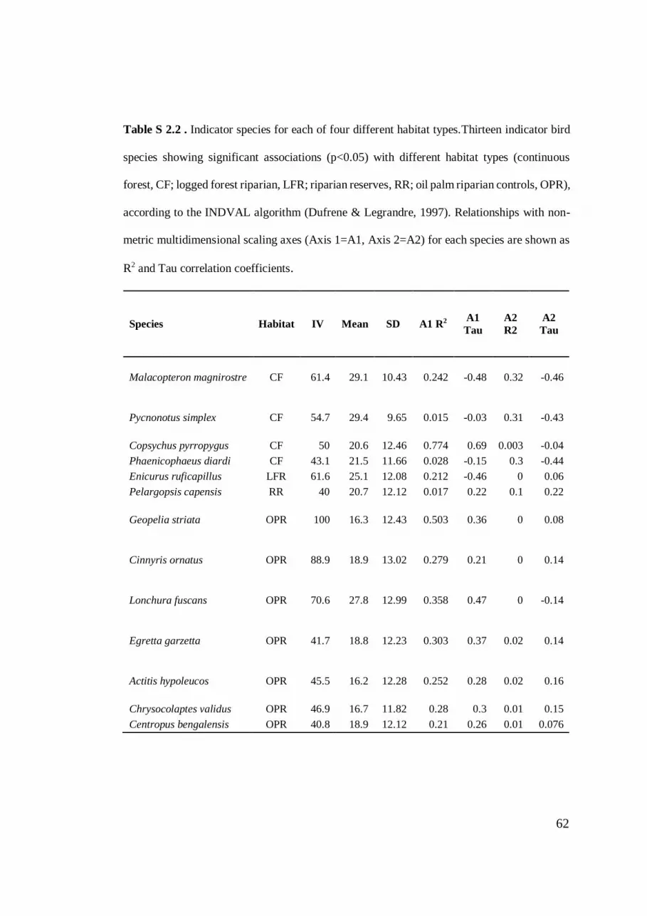
62
Table S 2.2 . Indicator species for each of four different habitat types.Thirteen indicator bird
species showing significant associations (p<0.05) with different habitat types (continuous
forest, CF; logged forest riparian, LFR; riparian reserves, RR; oil palm riparian controls, OPR),
according to the INDVAL algorithm (Dufrene & Legrandre, 1997). Relationships with non-
metric multidimensional scaling axes (Axis 1=A1, Axis 2=A2) for each species are shown as
R2 and Tau correlation coefficients.
Species Habitat IV Mean SD A1 R2 A1
Tau
A2
R2
A2
Tau
Malacopteron magnirostre CF 61.4 29.1 10.43 0.242 -0.48 0.32 -0.46
Pycnonotus simplex CF 54.7 29.4 9.65 0.015 -0.03 0.31 -0.43
Copsychus pyrropygus CF 50 20.6 12.46 0.774 0.69 0.003 -0.04
Phaenicophaeus diardi CF 43.1 21.5 11.66 0.028 -0.15 0.3 -0.44
Enicurus ruficapillus LFR 61.6 25.1 12.08 0.212 -0.46 0 0.06
Pelargopsis capensis RR 40 20.7 12.12 0.017 0.22 0.1 0.22
Geopelia striata OPR 100 16.3 12.43 0.503 0.36 0 0.08
Cinnyris ornatus OPR 88.9 18.9 13.02 0.279 0.21 0 0.14
Lonchura fuscans OPR 70.6 27.8 12.99 0.358 0.47 0 -0.14
Egretta garzetta OPR 41.7 18.8 12.23 0.303 0.37 0.02 0.14
Actitis hypoleucos OPR 45.5 16.2 12.28 0.252 0.28 0.02 0.16
Chrysocolaptes validus OPR 46.9 16.7 11.82 0.28 0.3 0.01 0.15
Centropus bengalensis OPR 40.8 18.9 12.12 0.21 0.26 0.01 0.076

63
Acknowledgements
This study was funded by the UK Natural Environment Research Council (NERC)
(NE/K016407/1; http://lombok.hmtf.info/ and http://bali.hmtf.info; NE/K016377/1),
and a Newton-Ungku Omar Fund grant from the British Council and Malaysia
Industry-Group for High Technology (MIGHT) (216433953). SLM was supported by
a PhD scholarship jointly funded by University of Kent and NERC. We thank the
Sabah Biodiversity Council, Sabah Forest Department, Yayasan Sabah, Sime Darby,
Benta Wawasan, Sabah Softwoods and Innoprise Foundation for permitting site
access. We are grateful to Unding Jami and the LOMBOK research assistant team for
their field assistance, and Suzan Benedick, Joseph Tobias and Ryan Gray for
facilitating fieldwork.
References
Analytics Revolution. ‘doMC: For each parallel adaptor for the multicore package.’ R
package version 1.3.
Azhar, B., Lindenmayer, D.B., Wood, J., Fischer, J., Manning, A., McElhinny, C. &
Zakaria, M. (2011) The conservation value of oil palm plantation estates,
smallholdings and logged peat swamp forest for birds. Forest Ecology and
Management, 262, 2306–2315.
Banks-Leite, C., Pardini, R., Tambosi, L. R., Pearse, W. D., Bueno, A. A., Bruscagin,
R. T., ... & Metzger, J. P. (2014). Using ecological thresholds to evaluate the costs
and benefits of set-asides in a biodiversity hotspot. Science, 345(6200), 1041-
1045.

64
Bueno, A. S., Bruno, R. S., Pimentel, T. P., Sanaiotti, T. M., & Magnusson, W. E.
(2012) The width of riparian habitats for understory birds in an Amazonian
forest. Ecological Applications, 22(2), 722-734.
Bivand, R. & Rowlingson, B. (2016) Package ‘rgdal.,’ R Package.
doi:10.1353/lib.0.0050.e.
Bivand, R. & Lewin-Koh, N. ‘maptools: Tools for reading and handling spatial
objects.’ R package version 0.8–27.Chan, E.K.W, Chan, E. K., Yu, Y. T., Zhang,
Y., & Dudgeon, D. (2008) Distribution patterns of birds and insect prey in a
tropical riparian forest. Biotropica, 40, 623-629.
Capon, S.J., Chambers, L.E., Mac Nally, R., Naiman, R.J., Davies, P., Marshall, N, …
Baldwin, D.S. (2013) Riparian ecosystems in the 21st century : Hotspots for
climate change adaptation? Ecosystems, 16, 359–381.
Dixon, P. (2003) ‘VEGAN, a package of R functions for community ecology.’ Journal
of Vegetation Science, 14(6), 927–930.
da Silva, N. M., Angeoletto, F., Santos, J. W., Paranhos Filho, A. C., Vacchiano, M.
C., Bohrer, J. F., & Cândido, A. K. A. (2017). The negative influences of the new
brazilian forest code on the conservation of riparian forests. European Journal of
Ecology, 3(2), 116-122.
de Fraga, R., Lima, A., P. and Magnusson W., E.Mesoscale spatial ecology of a
tropical snake assemblage: the width of riparian corridors in central Amazonia.
(2011) The Herpetological Journal 21(1) 51-57.
Dufrene, M. and Legendre, P. (1977) Species assemblages and indicator species : The
need for a flexible asymmetrical approach, Ecological Monographs, 67, 345–
366.

65
Eaton, J.A., van Balen, B., Brickle, N.W. & Rhiendt, F.E. (2016) Birds of the
Indonesian Archipelago. Lynx Editions
Edwards, D.P., Hodgson, J.A., Hamer, K.C., Mitchell, S.L., Ahmad, A.H., Cornell,
S.J. & Wilcove, D.S. (2010) Wildlife-friendly oil palm plantations fail to protect
biodiversity effectively. Conservation Letters, 3, 236–242.
Ewers, R.M., Thorpe, S. & Didham, R.K. (2007) Synergistic interactions between
edge and area effects in a heavily fragmented landscape. Ecology, 88, 96–106.
Ewers, R.M., Didham, R.K., Fahrig, L., Ferraz, G., Hector, A., Holt, R.D, … Turner,
E.C. (2011) A large-scale forest fragmentation experiment: the Stability of
Altered Forest Ecosystems Project. Philosophical Transactions of the Royal
Society B: Biological Sciences, 366, 3292–3302.
Giam, X., Hadiaty, R.K., Tan, H.H., Parenti, L.R., Wowor, D., Sauri, S, … Wilcove,
D.S. (2015) Mitigating the impact of oil-palm monoculture on freshwater fishes
in Southeast Asia. Conservation Biology, 29, 1357–1367.
Gibbs, H.K., Ruesch, A.S., Achard, F., Clayton, M.K., Holmgren, P., Ramankutty, N.
& Foley, J.A. (2010) Tropical forests were the primary sources of new
agricultural land in the 1980s and 1990s. PNAS, 107, 1–6.
Gibson, L., Ming Lee, T., Koh, L.P., Brook, B.W., Gardner, T.A., Barlow, J, … Sodhi,
N.S. (2011) Primary forests are irreplaceable for sustaining tropical biodiversity.
Nature, 478, 378–381.
Gillies, C.S., Cassady, C. & Clair, S. (2008) Riparian corridors enhance movement of
a forest specialist bird in fragmented tropical forest. PNAS, 105, 19774–19779.
Gilroy, J. J., and Edwards, D. P., (2017) Source-sink dynamics: a neglected problem
for landscape-scale biodiversity conservation in the tropics. Current Landscape
Ecology Reports 2(1), 51-60.
66
Government of Malaysia. (1965) National Land Code (No. 56 of 1965).
Gray, C.L., Slade, E.M., Mann, D.J. & Lewis, O.T. (2014) Do riparian reserves
support dung beetle biodiversity and ecosystem services in oil palm-dominated
tropical landscapes? Ecology and Evolution, 4, 1049–60.
Gray, C.L., Simmons, B.I., Fayle, T.M., Mann, D.J. & Slade, E.M. (2016) Are riparian
forest reserves sources of invertebrate biodiversity spillover and associated
ecosystem functions in oil palm landscapes? Biological Conservation, 194, 176–
183.
Hansen, M. C., Stehman, S. V., & Potapov, P. V. (2010). Quantification of global
gross forest cover loss. PNAS, 107(19), 8650-8655.
Hansen, M. C., Potapov, P. V., Moore, R., Hancher, M., Turubanova, S., Tyukavina,
A., ... & Kommareddy, A. (2013). High-resolution global maps of 21st-century
forest cover change. Science, 342(6160), 850-853.
Hijmans, R.J. & van Etten, J. Raster: Geographic analysis and modelling with raster
data. R package version 2.0-12.
IUCN 2017. The IUCN Red List of Threatened Species. Version 2017-3.
<http://www.iucnredlist.org>.
Jucker, T., Asner, G. P., Dalponte, M., Brodrick, P., Philipson, C. D., Vaughn, N.,
…& Coomes, D. A. (2018) Estimating aboveground carbon density and its
uncertainty in Borneo’s structurally complex tropical forests using airborne laser
scanning, Biogeosciences Discuss, https://doi.org/10.5194/bg-2018-74, in
review.
Kitzes, J., & Hartle, J. (2015) Predicting extinction debt from community patterns.
Ecology, 96, 2127–2136.

67
Laurance, W.F., Carmargo, J.L.C., Fearnside, P.M., Lovejoy, T.E., Williamson, B.G.,
Mesquita, R.C.G, … Laurance, S.G.W. (2018) An Amazonian rainforest and its
fragments as a laboratory of global change. Biological Reviews, 93, 223–247.
Lees, A.C. and Peres, C. A. (2008) Conservation value of remnant riparian forest
corridors of varying quality for amazonian birds and mammals. Conservation
Biology, 22, 439.
Luke, S., Slade, E., Drewer, J., Annamala, V., Mitchell, S.L., Williamson, J, …
Struebig, M.J. (2018) Riparian buffers in tropical agriculture: scientific support,
effectiveness and directions for policy. Journal of Applied Ecology. (Submitted:
BioRxiv ID…)
Mayer, P., Reynolds, S.K.J., McCutchen, M.D. & Canfield, T.J. (2007) Meta-Analysis
of nitrogen removal in riparian reserves, Journal of Environmental Quality, 36,
1172–1180.
McCune, B. & Mefford, M.J. (2011) PC-ORD. Multivariate analysis of ecological
data. Version 6.07
Pebesma, E., & Bivand, R. S. (2005). S classes and methods for spatial data: the sp
package. Unpublished report.
ftp://200.236.31.2/CRAN/web/packages/sp/vignettes/intro_sp.pdf
Pimm, S.L., Jenkins, C.N., Abell, R., Brooks, T.M., Gittleman, J.L., Joppa, L.N., …
& Sexton, J.O. (2014) The biodiversity of species and their rates of extinction,
distribution, and protection. Science, 344, 1246752.
Round, P., Gale, G.A. & Brockelman, W.Y. (2006) A comparison of bird communities
in mixed fruit orchards and natural forest at Khao Luang, southern Thailand.
Biodiversity and Conservation, 15, 2873–2891.

68
Sabah State Government (1968) Forest enactment 1968
http://www.lawnet.sabah.gov.my/lawnet/sabahlaws/StateLaws/ForestEnactment
1968.pdf
Sabo, J.L., Sponseller, R., Dixon, M., Gade, K. & Harms, T, Heffernan, J., … Welter,.
J. (2005) Riparian zones increase regional species richness by harboring
different, not more, species. Ecology, 86, 56–62.
Schietti, J., Emilio, T., Rennó, C. D., Drucker, D. P., Costa, F. R., Nogueira, A., ... &
Guillaumet, J. L. (2014). Vertical distance from drainage drives floristic
composition changes in an Amazonian rainforest. Plant Ecology &
Diversity, 7(1-2), 241-253.
Struebig, M.J., Turner, A., Giles, E., Lasmana, F., Tollington, S., Bernard, H. & Bell,
D. (2013) Quantifying the biodiversity value of repeatedly logged rainforest:
Gradient and comparative approaches from Borneo. Advances in Ecological
Research, 48, 183–224.
van der Hoek, Y., Zuckerberg, B., & Manne, L. L. (2015). Application of habitat
thresholds in conservation: Considerations, limitations, and future
directions. Global Ecology and Conservation, 3, 736-743.
Vijay, V., Pimm, S., Jenkins, C. N., & Smith, S.J. (2016). The impacts of oil palm on
recent deforestation and biodiversity loss. PLOS ONE,
https://doi.org/10.1371/journal.pone.0159668
Warren-Thomas, E., Dolman, P.M. & Edwards, D.P. (2015) Increasing demand for
natural rubber necessitates a robust sustainability initiative to mitigate impacts on
tropical forest, Conservation Letters, 8, 230–241.
Weldon, A.J. & Haddad, N.M. (2017) The effects of patch shape on indigo buntings :
Evidence for an ecological trap, Ecology, 86, 1422–1431.

69
Wilson, M. F., O’Connell, B., Brown, C., Guinan, J. C., & Grehan, A. J. (2007).
Multiscale terrain analysis of multibeam bathymetry data for habitat mapping on
the continental slope. Marine Geodesy, 30(1-2), 3-35.
Yaap, B., Magrach, A., Clements, G. R., McClure, C. J., Paoli, G. D., & Laurance, W.
F. (2016). Large mammal use of linear remnant forests in an industrial pulpwood
plantation in Sumatra, Indonesia. Tropical Conservation Science, 9(4),
1940082916683523.
Zimbres, B., Peres, C.A. & Bom, R. (2017) Terrestrial mammal responses to habitat
structure and quality of remnant riparian forests in an Amazonian cattle-ranching
landscape, 206, 283–292.

70
Species traits predict thresholds of
nonlinear response to forest change
Simon L. Mitchell1, Nicholas J. Deere1, David P. Edwards2, Thomas Swinfield3,
David Milodowski4, James Gilroy5, David Coomes3, Henry Bernard6, Joseph
Tobias7, Zoe G. Davies1, Matthew J. Struebig1
1Durrell Institute of Conservation and Ecology (DICE), School of Anthropology and
Conservation, University of Kent, Canterbury, Kent, CT2 7NR, UK
2 Department of Animal and Plant Sciences, University of Sheffield, Sheffield,
3Forest Ecology and Conservation Group, Department of Plant Sciences, University
of Cambridge, Cambridge, United Kingdom
4 School of GeoSciences, University of Edinburgh, Edinburgh, United Kingdom.
5School of Environmental Sciences, University of East Anglia, Norwich United
Kingdom
6Institute for Tropical Biology and Conservation, Universiti Malaysia Sabah, Kota
Kinabalu, Sabah, Malaysia
7Faculty of Natural Sciences, Department of Life Sciences, Imperial College London
Manuscript in preparation

71
Abstract
In the context of rapid environmental change it is import to understand how
state-shifts in ecosystems manifest via changes to ecological communities at the
species and functional levels. Assessing these patterns may be particularly useful for
predicting abrupt thesholds or ‘tipping points’ in ecological responses after which
ecosystems are more vulnerabale to collapse. Here, we assess the responses of 171
tropical birds species to environmental changes associated with forest degradation by
applying occupancy modelling to field ornithological data, together with habitat
structure information from hyper-spectral LiDAR. Across a land-cover gradient of
intact forest to oil palm plantations, we demonstrate that the majority of species
respond to habitat degradation in a non-linear fashion. These abrupt responses in
species occupancy scale up to abrupt changes to the composition of trait groups
associated with ecosystem functions such as pollination, seed dispersal and
insectivory. We show that disturbance responses at the trait-group level do not
necessarily follow threshold levels of all component species, since many species have
idiosyncratic responses. Nonetheless, several trait groups exhibit markedly differing
threshold levels from one another, for example the frugivores and nectarivores
responded more strongly until canopy height reached 10 – 18 m, whereas both
terrestrial and sallying insectivores continued to respond strongly until canopy height
reach ~24 m. This suggests that, just as trait-based approaches have proven useful in
generalising overall effects in a linear framework, they offer a potentially useful way
of generalising non-linear response thresholds and that traditional analyses have
masked important species-specific and trait-group responses. These responses
demonstrate that passing particular thesholds could result in disproportionate losses of

72
biodiversity in human-modified tropical landscapes Our findings suggest that the use
of non-linear response models offer a framework to reduce false-negative errors in
detecting species responses, optimise indicator species used for particular trait groups
and understanding fine-scale habitat assocations, especially for highly specialised
species.
Introduction
Global environmental changes are causing mass species extinctions (Ceballos
et al., 2015) and increasing the vulnerability of ecosystems to collapse (Scheffer et al.,
2001; Cardinale et al., 2012). In terrestrial ecosystems, the leading cause of these
processes is direct anthropogenic modification of vegetation through landuse change,
including habitat conversion, degradation and fragmentation (Ellis, 2011; Newbold et
al., 2015). An extensive literature has established links between shifts in ecological
communities and landuse change (Gerstner et al., 2014), forest degradation (Gibson
et al., 2011) and habitat configuration (Haddad et al., 2015), with many species being
reduced in abundance as a consequence of these activities (Phalan, 2011), but a few
increasing significantly (Deviktor et al., 2008). Given the enormous global impacts
that habitat alterations can have on biodiversity and the functions and services that
biodiversity provides, further scrutiny of how land-cover change processes influence
species is paramount to conservation.
Functional ecology frameworks allow predictions about how whole groups of
species shift by measuring associations between species ecological traits and their
responses to environmental change. For example, poorer dispersal capability and
larger body size predict range contraction in butterflies (Mattila et al., 2011), and life-
history strategies associated with greater specialisation predict greater sensitivity to

73
landuse change for dung-beetles (Barragán et al., 2011), and birds (Newbold et al.,
2013), as well as increased extinction risk in birds (Sekercioglu et al., 2007), terrestrial
mammals (Davidson et al., 2009), and bats (Jones et al., 2003). Traits have also been
shown to mediate the effects of particular drivers of decline, such those induced by
the novel the Chytridiomycosis pathogen in amphibians (Murray et al., 2010), or by
climate change in amphibians, reptiles (Pearson et al., 2014) and birds (Pacifici et al.,
2017). Trait-based approaches are also useful in predicting patterns of ecosystem
function (Lavorel & Garnier, 2002). However, to date, trait-based approaches have
focussed predominantly on simple linear associations between trait and response (e.g
Williams et al., 2010; but see Sasaki et al., 2011) or upon changes in overall functional
diversity, which is assessed based on the overall diversity and representation of
multiple traits within a community (Magioli et al., 2014). To fully understand the
responses of different trait groups, assessments need to take account of both the
variation of responses between member species of particular trait groups, and the
potential for those responses to be non-linear.
Relationships between changes in environment and subsequent responses of
communities and ecosystems are frequently non-linear (Groffman et al., 2006;
Andersen et al., 2009). The associated inflection points may constitute critical
thresholds beyond which more abrupt, often irrevocable, changes can occur (Scheffer
et al., 2001). Such ‘state shifts’ can occur at the ecosystem, community and species
levels. For example, sudden transitions between tropical forest and savannah
ecosystems, are associated with small changes in precipitation (Hirota et al., 2011);
abrupt changes in community-level responses to habitat loss for bats (Muylaert et al.,
2016), reptiles (Lindenmayer et al., 2005), amphibians (Riley et al., 2005), mammals
74
(Silva et al., 2005) and birds (Martensen et al., 2012); and some bird temperate species
exhibit thresholds in their response to habitat loss (Radford & Bennet 2004; Betts et
al. 2007). However, these studies focus either on a few detailed species responses, or
in patterns of overall richness. As yet, no assessments have been made that
demonstrate the relative contribution of each species response to producing non-linear
patterns at the level of the whole community.
Identifying such thresholds in ecological processes and ecosystem responses
could have profound implications for the ways the environment is managed. In the
context of the global biosphere, exceeding dangerous thresholds may in fact present
an existential threat to human civilisation (Rockstrom et al., 2009). Furthermore,
ecosystems and functions may become difficult or impossible to restore once certain
thresholds are crossed (e.g. Carpenter et al., 1999). Applying information from
thresholds in diversity responses to landscape change has useful applications for
conservation planning, as demonstrated for Atlantic forest birds (Banks-Leite et al.,
2014). However, examining species numbers alone misses important information on
ecological processes that tend to manifest at lower hierarchical levels, building from
individuals, to species, to communities, to ecosystem processes (DeAngelis 2018).
The extent of, and way in which, thresholds in ecological responses scale between
these different levels is poorly understood. Understanding non-linear responses at the
levels of species, guilds and communities is therefore a vital underpinning of our
ability to recognise how species can be maintained at the levels of landscapes to global
ecosystems.
There are a number of impediments faced in assessing how species response
thresholds scale to functional groups and community richness. Compared to traditional

75
assessments that simply seek to demonstrate the existence and direction of species
responses to environmental change, identifying thresholds in these responses requires
far larger datasets of a high resolution for each species as well as relevant
environmental metrics. Statistical approaches to address this have been proposed
(Baker & King, 2010), but remain contentious (Cuffney & Qian, 2013). Occupancy
modelling approaches may help overcome data limitations concerning rarer species by
controlling for imperfect detection. However, occupancy approaches have been used
in very few threshold studies to date (e.g. Betts et al., 2010). Traditional remote
sensing techniques can expedite the gathering of large datasets on landscape-scale
environmental gradients, but in the past have generally been limited to fairly
rudimentary two-dimensional landscape-scale measurements. Landscape metrics have
been used in the majority of community threshold studies thus far, resulting in a clear
emphasis upon responses to landscape configuration and habitat loss within the
literature (Melo et al., 2018).
Despite the focus on landscape-scale factors, abrupt declines in species
richness have also been documented with small increases in habitat disturbance
intensity for dung beetles (Franca et al., 2017), and in response to changes in nutrient
levels and turbidity for aquatic invertebrates (e.g. Evans-White et al., 2008),
suggesting similar non-linear responses to fine-scale habitat characteristics and
structural properties also exist. To better examine tipping points in relation to the
structural properties of tropical forests, utilising data from remote-sensed Light
Detection and Ranging (LiDAR) offers a promising way forward. Hyper-spectral
LiDAR provides the ability to map the fine-scale structure of vegetation in three

76
dimensions and so offers the potential to analyse patterns of faunal distribution and
association which were previously unachievable.
Here, we couple occupancy modelling across multiple species with data
derived from high resolution LiDAR to examine thresholds in the effects of 3D
structure and landscape metrics associated with tropical forest degradation. Where
previous studies have focused on single species (Garabedian et al., 2017), we assess
thresholds in response at the level of species, trait-groups and entire communities
simultaneously. Using a large dataset (n = 1404 point counts) of bird observations as
an established indicator taxon (Gardner et al., 2008), we are able to trace how abrupt
responses of individual taxa contribute to thresholds among trait groups, ensembles
and the community at large. We explore whether each species responses is better
predicted with or without a threshold included in the model. The responses of species
with shared traits to environmental gradients are often similar, as trait-group members
respond similarly to a single underlying mechanism, such as the availability of a
particular niche (e.g. Williams et al., 2010). This suggests that species with shared
traits will not only demonstrate similar responses to environmental changes, but that
where these responses are non-linear, they also exhibit similar threshold levels.
Materials and methods
Study system
Between 2010 and 2017, we sampled bird communities via repeated point
counts at 356 localities across a gradient of habitat degradation in the dipterocarp
forests of Sabah, Borneo (Fig. 3.1). Old growth forest was sampled at 47 point count

77
localities across three landscapes at Sepilok Forest Reserve (19 localities), Danum
Valley (20) and Maliau Basin (8). The majority of point count localities (309) were
located around the Stability of Altered Forest Ecosystem (SAFE) project landscape.
Of these, 38 were in continuous forest of the Ulu Segama Forest Reserve, which was
logged twice since the 1970s, but now protected and recovering. The remaining 156
localities were in the neighbouring SAFE landscape in forest that had been logged
several times since the 1970s and salvage-logged ahead of conversion to plantation. A
further 115 localities comprised forest remnants within two large oil palm estates
surrounding the SAFE project area. This provided respresentative sampling across the
complete range of environmental variables we assessed. Sample sites were a minimum
of 180 m apart, and grouped into transects of 8-16 point count locations (see Chapter
2; Mitchell et al., 2018; Fig. 2.1).

78
Figure 3.1. Map of Sabah showing four study landscapes. Forest cover is shown in a
green. The darkest pixels represent the highest carbon densities (maximum: 303.98),
and the palest areas associated with the lowest carbon forest (minimum: 0); plantation
areas also are masked in white. Carbon density is derived from Asner et al., (2018).
The SAFE landscape and surrounding area (inset) show the detailed configuration of
points. Red dots indicate sampling locations.
Bird sampling
Each point count locality was sampled three to five times by a single
experienced observer (SLM or DPE) who recorded all bird species seen or heard
within a 50 m radius of a stationary position for 15 minutes, including fly-overs.

79
Counts were conducted between 05:50 and 11:00, on mornings without rain or high
winds. The 50 m radius around the points comprised a range of habitat types, including
both entirely and partly forested habitat, oil palm plantations, rivers channels, bare
ground and early regenerating tropical scrub. Counts were recorded and a random sub-
sample of recordings later re-checked to ensure species were not overlooked.
LiDAR-based forest structure and configuration predictors
Across all sites we generated five metrics from remotely-sensed data to
quantify forest structure and configuration. Four measures were derived from LiDAR
point clouds gathered in November 2014 using a Leica ALS50-II sensor (Jucker et al.
2018), and reflected mean values within a 50 m radius of each sampling locality. We
quantified mean canopy height as well as the standard deviation in canopy height (as
a measure of structural heterogeneity). To avoid multicollinearity with canopy height,
we included plant area index per metre canopy height, giving an effective measure of
vegetation density. We also quantified skewness of the vertical distribution of
vegetation density. Finally, as a measure of landscape-scale habitat availability, we
included the proportion of forest cover within 100 m radius of each point count,
extracted from the forest cover layer produced by Gaveau et al., (2014), using the
classification of multiple land cover data sources. There was no strong correlation
between these five variables - Variance Inflation Factors in relation to canopy height
were all below four (canopy heterogeneity, 1.32; plant area density, 1.23; skew, 1.22;
forest cover, 1.11).

80
Occupancy modelling
To model avian responses to habitat degradation, we constructed multispecies
hierarchical occupancy models. Community models are comprised of multiple single
species occupancy-detection models that hierarchically partition the ecological and
sampling processes underpinning the data to differentiate true absence from non-
detection (Dorazio & Royle, 2005; Deere et al., 2017). Single-species models were
linked via an additional hierarchical component that modelled community-level
regression coefficients from a common distribution with estimable hyper-parameters.
Consequently, species responses are partially informed by the community average,
which provides more robust parameter estimates for rare species that are infrequently
detected during sampling (Pacifici et al., 2014). This means that species have similar,
but not identical, environmental responses across the community. To reduce model
uncertainty, we excluded 35 species that were detected at fewer than three sites, as
changes in occupancy and detection cannot be reliably uncoupled when detection data
are this sparse, thus resulting in a total community of 171 species (Table S3.1,
Supporting information). Whilst this results in the exclusion of the rarest species,
community occupancy models necessarily involve a trade off between representing as
many species as possible and excluding species for which there is insufficient data to
make robust inferences. A further assumption is that variation in abundances do not
effect species detection probabilities (Royle & Dorazio, 2008).
Our multispecies model controlled for the effects of date and time-of-day. We
applied the R function ‘scale’ (R Core Team, 2014) to standardise our five predictor
variables and two detection variables (using root-mean-squares) prior to analysis. This
was undertaken to ensure that the influence of different variables upon a species

81
occupancy could be properly compared. Occurrence probabilities were modelled for
each species i at each point count site j via a logit link function:
𝐿𝑜𝑔𝑖𝑡 (𝜑𝑖,𝑗) = 𝛼𝑖,𝑠 + 𝛽1𝑖 ∙ canopy height𝑗 + 𝛽2𝑖 ∙ canopy heterogeneity𝑗 + 𝛽3𝑖
∙ skew𝑗 + 𝛽4𝑖 ∙ density𝑗 + 𝛽5𝑖 ∙ forest cover𝑗
Our multispecies model was then fitted to an observation matrix 𝑋𝑖,𝑗,𝑘 . This
reflects the number of occasions on which each species i was detected at each site j on
each visit k of the total number of visits (K). By specifying our observed data as the
sum of K Bernoulli trials with detection probability 𝜃𝑖,𝑗,𝑘 we estimated true
occurrences 𝑧𝑖,𝑗 as follows:
𝑋𝑖,𝑗,𝑘 ~ Bern (𝜃𝑖,𝑗,𝑘 ∙ 𝑧𝑖,𝑗)
To account for greater detectability associated with higher avian activity
around dawn, we modelled standardised time as influencing detection probability.
Similarly, as our study took place across multiple seasons, we included standardised
date as a parameter. This also allowed us to model occupancy without directly
accounting for potential immigration and emigration of birds to/from sites. Detection
probability was modelled for each species 𝜃 with a logit link function:
𝐿𝑜𝑔𝑖𝑡 (𝜃𝑖,𝑗,𝑘) = 𝜆𝑖,𝑠 + 𝛽7𝑖 ∙ 𝑡𝑖𝑚𝑒𝑗,𝑘 + 𝛽8𝑖 ∙ date𝑗,𝑘
Using a Bayesian framework we specified three Markov chains per parameter,
consisting of 120,000 iterations, with a burn-in of 30,000 iterations and thin rate of 10.
We assigned diffuse uniform priors for hyper-parameter means and inverse-gamma
priors for hyper-parameter variances (Dorazio et al. 2006) in order to provide an
uninformative start point that made no assumption or use of a priori occupancy
82
estimates. Our models were fitted using JAGS v4.3.0 (Plummer, 2017) and called in
R with “rjags” (Plummer, 2013), using the wrap-around “jagsUI” (Kellner 2015). We
confirmed convergence numerically by inspecting Bayesian P values and lack of fit
statistics for each species.
We compared species occupancy probabilities to each of our five
environmental variables. Effect sizes of each variable upon each species were assessed
in the occupancy model. For community-level effect sizes we measured the
community-level hyper-parameter for each metric, which is an averaged effect size
informed by all species, weighted according to the number of times they were detected
(i.e. abundant species contribute more than rare species).
Testing for thresholds in species response to forest structure and configuration
We identified thresholds in occupancy response to the environmental
covariates using the R package ‘segmented’ (Muggeo, 2008), which identifies the
point of maximum likelihood of a break in otherwise linear relationships. To test for
breakpoints between each species occupancy response and each of our five predictor
variables, we used 100 random draws of estimated occupancy probability for each
species across all 356 sites. For every species i, we regressed each random draw m of
all 356 sites against each of our five independent variables x. For each random draw,
we used segmented logistic regression (Muggeo, 2003) to test for a single break point
(threshold) 𝜑 where (𝑥 − 𝜑)+ = (𝑥 − 𝜑)𝑋𝐼(𝑥 − 𝜑). The intercept 𝛽0, slope of left
line 𝛽1 and difference between the slopes 𝛽2 were estimated through an iterative
process of fitting following the equation:

83
�̂� = exp (𝛽0 + 𝛽1𝑥 + 𝛽2 (𝑥 − 𝜑)+
1 + exp (𝛽0 + 𝛽1𝑥 + 𝛽2 (𝑥 − 𝜑)+))
For each draw m, we also obtained confidence intervals around the maximum
likelihood estimate for each threshold 𝜑, via linear approximation of the ratio of two
random variables via the delta method (Muggeo 2003; Betts et al., 2003) and derived
Akaike Information Criterion (AIC) values to measure the relative quality of each
model. We repeated both these processes for 100 samples M of each species i. This
provided us with mean thresholds, mean confidence intervals, and mean AIC of 100
samples for each species:
�̅�𝑖 =
(�̂� = exp (𝛽0 + 𝛽1𝑥 + 𝛽2 (𝑥 − 𝜑)+
1 + exp (𝛽0 + 𝛽1𝑥 + 𝛽2 (𝑥 − 𝜑)+)))𝑚
𝑀 𝑖
For each sample m we also computed a linear regression, which calculated
AIC. To determine whether our segmented model represented an improvement, we
compared mean AIC of M samples between our linear and segmented models. Any
species where AIC was not reduced by >4 was considered to be better represented by
a model without a break point. Species which did not show thresholds were excluded
from further analyses regarding the average level of thresholds (Fig. S3.6), but
retained within analyses assessing cumulative trait-group responses (Fig. 3.2 - 3.5).
We assumed only a single break-point for each species in order to allow for coherent
summarising of threshold patterns to group level. To ascertain cumulative group
response thresholds and confidence intervals (and trait group averages – see later), we
performed a single segmented linear regression on all samples M of all species I within
each trait group t. Since the initial value 𝜑 has the potential to influence the value of
maximum likelihood of a break-point (Muggeo, 2003), we defined the initial value of

84
𝜑 as the mean of each environmental metric. We compared this to break-point tests
with 𝜑 taken via random draws from a uniform distribution of full environmental
range, which made no discernible difference. Bayesian piecewise regression (Hutter
2005) could, in theory, be performed within the occupancy model itself. However,
nesting a further iterative fitting process to an already computational intensive model
was not feasible.
Species trait groups
To assess the responses and non-linear thresholds of different trait groups we
employed two approaches. First, we aggregated both the effects and thresholds of all
species which showed non-linear responses and estimated the median and quartile
distributions for each group (Fig. S3.6). Separately, we added the responses of all
species in each trait group (including those with linear responses) and calculated
break-points in overall group responses (Fig. 3.2). We used three categories of species
groups relating to feeding guilds as well as associations with habitat and vegetation
strata. Each species was defined as a member of only one particular group within each
category, ensuring maximum differentiation of group. We examined the thresholds
associated with 18 ecologically relevant trait groups. Three groups comprised
inventories of association with vertical strata following Chapman et al., (2017), but
were edited with reference to del Hoyo et al., (2018) to make groups non-overlapping
and reflect only primary associations. Habitat association comprised the same species
lists defined for Borneo by Styring et al., (2007), whilst feeding guilds were those used
by Sheldon et al. (2010) (Table S3.3; Supporting Information). These authors used

85
additional trait groups which we also assessed, but we do not report averages or
thresholds for groups with fewer than four member species.
Deriving group-level richness from occupancy models
For each site, we calculated the estimated richness of each trait group as the
sum of the median occupancy probability from 1000 random draws of estimated
occupancy probability for each species in the group. To assess whether the average
thresholds of member species within each group, and thresholds for cumulative group
richness were associated, we performed correlation tests in R. Thresholds in group
richness were calculated using the R package ‘segmented’ (R Core Team, 2014) to
assess their relationship to canopy height and forest cover. This followed the same
methods as for individual species
Results
Effect sizes of occupancy responses to forest cover and structure
Community-average effects of environmental variables were largest for forest
cover (0.379; C.I. 0.217-0.5434), followed by canopy height (0.293; C.I 0.117–0.477),
vegetation density (0.174; C.I. 0.05-0.292) and skew (0.158, C.I. 0.054-0.260).
Canopy heterogeneity showed no significant average effect across the whole
community (0.068; C.I. -0.013-0.147). Of the 171 species included within our
occupancy model, we found significant positive effects of forest cover on the
occupancy of 36 species (i.e. 21% of the community more prevalent in forest), and
significant negative effects for 16 species (9% less prevalent in forest; Fig S3.2).

86
Occupancy of 44 species (26%) responded positively to canopy height, while 14 (8%)
responded negatively (Fig S3.1). Greater vegetation density led to increased
occupancy of 20 species (12%), but reduced occupancy for two species (1%; Fig.
S3.3), while 14 species were positively affected by canopy vegetation skewed towards
greater height, while none responded negatively (Fig S3.4). Three species (2%)
exhibited positive effects of canopy heterogeneity, whilst none showed a negative
effect (Fig S3.5). Although effect sizes varied greatly between species, we did not
detect clear differences between trait groups according to strata-association, feeding
guilds or habitat-association (Fig. S3.6).
Group richness effects and thresholds
The effects of canopy height and forest cover on occupancy-derived richness
varied between guilds, trait groups and habitat groups (Fig 3.2; Fig 3.3). Canopy height
and forest cover had consistently positive effects upon richness for all trait-group,
except in the case of edge species, for which richness was negatively associated with
both.
Table 3.1. Threshold levels in trait group richness. Threshold given for each different strata-
association groups, feeding guilds and habitat-association groups in relation to canopy height
(within 50 m radius) and forest cover (within 100 m radius) with median (Med) and 95% lower
(Lwr CI) and Upper (Upr CI) confidence intervals. ΔAIC values show the reduction in AIC
from linear models to segmented models.
Mean Canopy Height
in 50 m radius
Proportion forest cover
in 100 m radius

87
Group Med Lwr
CI
Upr
CI
ΔAIC Med Lwr
CI
Upr
CI
ΔAIC
Str
ata
Canopy
9.75 7.05 12.46 12.26 0.84 0.72 0.95 4.66
Understorey 25.61 21.70 29.52 21.03 0.62 0.53 0.71 49.23
Ground
25.33
19.94
30.74
9.13
0.81
0.69
0.92
8.45
Feedin
g g
uil
ds
Arboreal frugivore
18.83
15.81
21.86
37.10
0.74
0.66
0.82
42.18
Arboreal gleaning
insectivore
22.71
19.23
26.20
22.52
0.78
0.63
0.94
5.51
Arboreal gleaning
Insect / frugivore
29.41
21.64
37.19
4.10
0.78
0.73
0.84
55.90
Sallying insectivore
25.32
22.46
28.19
40.50
0.78
0.68
0.89
16.17
Terrestrial
insectivore
25.33
21.69
28.98
24.20
0.79
0.65
0.93
6.86
Terrestrial
insectivore. /
frugivore
42.75
33.37
52.14
6.18
0.78
0.62
0.94
5.15
Nectarivore / insectivore/
frugivore
10.08
8.209
11.96
20.85
0.79
0.66
0.91
10.58
Insectivore /
pescivore
35.45
29.39
41.51
17.67
0.74
0.68
0.81
56.05
Raptor
9.94
9.125
10.76
94.50
0.09
0.07
0.11
243.2
Ha
bit
at
ass
oci
ati
on
s
Forest-specialist
22.61
16.52
28.71
4.81
0.78
0.70
0.87
26.85
Edge-tolerant forest
25.52
19.70
31.34
7.51
0.77
0.69
0.85
30.49
Edge species
20.09
18.24
21.94
87.30
0.81
0.63
0.99
1.16
Open species
31.78
26.40
37.16
16.69
0.89
0.79
0.99
2.11
Generalist species
36.15
28.69
43.61
10.85
0.79
0.72
0.87
27.58
For canopy height and forest cover, trait groups demonstrated markedly
different response thresholds in richness (Table 3.1). For example, thresholds in group
richness differed between strata-association groups in relation to both canopy height
and forest cover (Fig. 3.2). Canopy species had the lowest threshold with canopy
height (median 9.75 m, C.I 7.05 m-12.46 m), followed by Ground species (25.33 m,

88
C.I 19.94 m–30.74 m) and Understorey species (25.61 m, C.I 21.70 m-29.52 m). The
change in the magnitude of response (i.e. the change in the steepness of the lines), was
also markedly different. Canopy species went from a rate for increase of ~1 additional
species per metre (spp./m) below the threshold to ~0.24 additional spp./m above the
threshold, Understorey species ~0.25 spp./m below the threshold to ~0.03 spp./m
above the threshold and Ground species went from ~0.25 spp./m below the threshold
to ~0.09 spp./m above (Fig. 3.2). Richness thresholds of different guilds also varied
in relation to canopy height (Fig. 3.3). However, group richness thresholds in relation
to forest cover were consistently around 73-78% of forest cover for feeding guilds
(with the exception of raptors; Table 3.1). Groups of species associated with different
habitat types exhibited somewhat differing thresholds in response to canopy height,
but either did not differ, or did not exhibit thresholds, in relation to forest cover (Table
3.1).

89
Figure 3.2. Species richness predicted by the segmented models for strata associations. Three
different groupings of species are reported depending on strata associations and related to both
mean canopy height and proportion of forest cover. Median occupancy values of each species
are used. Thresholds displayed are calculated from median values, with confidence intervals
(shaded) calculated by the segmented package in R. All segmented relationships are ΔAIC>4
improvement from linear models.

90
Figure 3.3. Species group richness predicted by the best segmented models for nine avian
feeding guilds. Richness reported in relation to mean canopy height. Median occupancy values
of each species are used. Thresholds are calculated from median values, with confidence
intervals (shading) calculated by the segmented package. All segmented relationships are
ΔAIC>4 improvement from linear models.

91
Figure 3.4. Segmented models for different species of the arboreal frugivore feeding
guild. Occupancy probability responses to mean canopy height, together with
predicted richness resulting from all eight species. Vertical lines denote species 95%
Bayesian credible intervals. Median occupancy values of each species are used for
predicted richness. Thresholds displayed calculated from median values, with

92
confidence intervals (shading) calculated by the segmented package. All segmented
relationships are ΔAIC>4 reduction from linear models.

93
Figure 3.5. Segmented model for different species within the arboreal gleaning
insectivores / frugivores guilds. Occupancy reponses shown in relation to proportion
of forest, together with predicted richness resulting from all twenty species.
94
Vertical lines denote species 95% Bayesian confidence intervals. Median occupancy
values of each species are used for predicted richness. Thresholds displayed calculated
from median values, with confidence intervals (shading) calculated by the segmented
packaged. Segmented relationships are ΔAIC>4 reduction from linear models.
Species thresholds
Occupancy changes in relation to environmental covariates were better
explained by segmented models than linear ones. Associations between species
occupancy (derived from our model) and forest cover were better explained by
segmented models with a single breakpoint than by linear models for 139 species (i.e.
for 139 of 171 species the segmented model yielded a reduction of >ΔAIC=4
compared to the linear model for the same dataset). The same was true for 166 species
for canopy height, 129 species for vegetation density, 120 species responses to skew,
and 151 species for canopy heterogeneity (Table S3.3). Average reductions in model
AIC were 54.6 for forest cover, 86.4 for canopy height, 33.1 in density, 17.6 in skew
and 56.6 in canopy heterogeneity.
Between groups, the average threshold levels in the responses of member
species (i.e., thresholds in each species response to a given environmental variable,
taken as the median across all group member species) did not differ significantly
between the various strata groups, feeding guilds or habitat groups. Separating
member species of trait groups into further sub-groups depending on whether their
overall response was positive or negative, or whether they showed increasing or
decreasing strength of response, did not highlight any significant variation between
trait-groups or sub-groups (Fig. S3.6; Table S3.5).

95
Thresholds of richness in relation to canopy height differed significantly
between different trait groups (Fig. 3.3), but were not correlated with the average
thresholds of the species within those groups (p=0.69). Nor were group richness
thresholds for forest cover associated with the median values for member species
thresholds (p=0.51).
Discussion
Our study demonstrates both variation and similarity in thresholds of species
responses to changes in forest cover and three dimensional structure - features known
to shift following tropical forest degradation. While the concepts of tipping points
(Folke et al., 2004) and non-linear responses (Meron, 2015) to environmental change
are fairly well established in the ecological literature, most observational studies
address these on broad scales, such as in the functioning of entire ecosystems (e.g
Nobre & Bourma, 2009), or changes of overall species richness or community
integrity (e.g. Banks-Leite et al., 2014). Our data on palaeotropical birds reveal a
number of tipping-points which appear to be common across multiple trait groups, but
also highlight idiosyncratic threshold levels for other species groups. We examined
the responses of almost every species in the bird community individually to discern
where unexpected responses of particular taxa might otherwise be overlooked by
grouping species together. Previous assessments that have tracked individual species
thresholds to their contribution to community-level effects either focussed on very
simple communities (Dieleman et al., 2015), selected groups of species (Betts et al.,
2010), or used species abundance (Suarez-Robio & Lookingbill, 2016) or naïve
occupancy (Bergman et al., 2004) as their response measure. Our study reveals how

96
thresholds in the responses of trait groups manifest, by examining how the differences
in thresholds between up to 48 different member species contribute to overall group
thresholds in richness. This multi-level examination allows us to address the efficacy
of applying the concept of thresholds to species trait groups.
Pervasive non-linear responses to habitat change in the tropical bird community
We found relationships between most species occupancy and environmental
variables were better described by models that included non-linear thresholds. Whilst
previous studies found individual species respond in a non-linear manner to two-
dimensional landscape scale changes (e.g. Betts et al., 2010), we assessed the
thresholds of responses to structural vegetation metrics, captured in three dimension
using hyperspectral LiDAR. Thresholds at the species level were most common in
responses to canopy height (Table 3.1). A few species also showed response
thresholds to explicitly three dimensional forest structure characteristics of skew and
vegetation density. For example, Blue-throated Bee-eater, Merops viridis increased in
occupancy probability with increased skew (vegetation density skewed towards the
higher vegetation strata). This was of a greater magnitude once skew increased above
a threshold of 0.9. Blue-throated Bee-eaters specifically hunt for insects from perches
on tall trees (del Hoyo et al., 2019), and prefer areas of mixed forest or open habitat
where vegetation is concentrated to higher canopy strata, since this maximises the area
of open storey where they predominantly forage. Conversely, other species (e.g.
Cream-vented Bulbul, Pycnonotus simplex) were only recorded in areas where skew
was below a threshold of 0.5. This species is described as favouring “lower and middle
storeys along forest trails, especially in more open areas” (del Hoyo et al., 2019),

97
which suggests that the species tolerates a maximum level of upwards vegetation
skew. The use of LiDAR data allows us to reveal several relationships like these across
a whole community for the first time.
Patterns in trait-group responses to forest disturbance
We found differing threshold levels in the 18 different trait groups we assessed,
both as member species-averages (Fig. S3.6), and when assessed as whole-group (Fig.
3.3; Fig 3.4). For example, principally nectarivorous species exhibited lower
thresholds in their response to canopy height than solely insectivorous guilds, both in
terms of member species averages (Fig. S3.6), and in the responses of group richness
derived from cumulative predicted occupancy (Fig. 3.3). Elsewhere on Borneo, Cleary
et al. (2007) demonstrated terrestrial insectivores to be more strongly negatively
affected by logging activities than nectarivores and frugivores, a finding associated
with reduced canopy height. We are able to elaborate on this assertion more
specifically by demonstrating that increases in canopy height from only 5 m to 10 m
result in an increase of 2-4 species detected (i.e. 0.4 additional species per metre
height). Once the canopy reaches 10 m in height, species richness gains are quite
minor: for example, an average of one nectarivorous bird for the next 50 m of
additional gain in canopy height (0.02 additional spp/m) (Fig. 3.3).
Contrary to this pattern, terrestrial insectivores increased at rate of 0.11
additional spp./m between 5 m and 25 m in canopy height (a much higher threshold
than nectarivores) after which only an average rate of 0.04 additional spp./m between
25 m and 60 m was observed (Fig. 3.3). Terrestrial insectivores have previously been
98
found to be largely absent from heavily logged forests (which are characterised by
reduced canopy height), apparently due to associated changes in microclimate and
leaf-litter (Stratford & Stouffer, 2012). By contrast, many principally nectarivorous or
frugivorous species are more abundant in logged forests (Cleary et al., 2010; Edwards
et al., 2009). Further to these basic ecological patterns, we can reveal specific,
contrasting cut-off points in canopy height below which terrestrial insectivores and
nectarivores decline at a more rapid rate.
Thresholds in the responses of feeding guilds to forest cover were remarkably
consistent, with eight out of nine feeding guilds showing abrupt changes in response
to forest cover at between 73% and 79%. Whilst this is higher than most previous
thresholds in the relationship between forest cover and overall community richness
(Melo et al., 2009), our higher threshold does not necessarily mean that feeding guilds
rapidly declined in species numbers once forest cover drops below ~75%. In fact,
increases in forest cover above 75% were associated with greater increases in species
richness than below this level. Since a number of forest specialist species across
several feeding guilds are known to exhibit strong preferences for forest interior
(Laurance, 2012), we suspect that the added contribution of these species, which are
absent in degraded or semi-open habitat (Peh et al., 2005), drive this pattern.
Inspecting the responses of forest specialist and edge tolerant forest species within
particular feedings guilds demonstrated this was the case. For example, Crested Jay
(Platylophus galericulatus), is defined as a forest specialist and Red-throated Barbet
(Psilopogon mystacophanos) as an edge-tolerant forest species (Styring et al., 2007),
but both are included within the Arboreal foliage-gleaning insectivore/frugivore guild.
Crested Jay occupancy increased slowly below 75% forest cover to 20% occupancy,

99
but after this threshold, increased more rapidly to 55% occupancy with 100% forest
cover. Similarly, Red-throated Barbet increased from 20% occupancy with 77% forest
cover to 50% occupancy with 100% forest cover (Fig. 5). Similar patterns were found
for each feeding guild where richness increased above a threshold of 70 – 80%.
The uncertainty around occupancy responses of individual species means that
thresholds generated from such interpolated data ought to be regarded with a degree
of caution. However, when species are accumulated together, such as in trait groups,
occupancy responses are supported by a greater number of both model samples and
species, such that inferences regarding abrupt changes in species’ occupancy
probability (which haven’t been nullified by variation of member species responses),
are more robust.
Idiosyncratic species responses
Trait groups are useful in generalising species responses to environmental
variables. However, relying solely upon trait groups may obscure patterns of
individual species responses (Laurance, 2012). Similarly, we found trait groups
provide a useful way of understanding the general patterns of community break-points,
but member species within groups should not necessarily be assumed to have similar
thresholds to one another. We found that in species trait groups, both the overall effects
and thresholds in responses for individual species were sometimes lost. For example,
arboreal frugivores showed no increase in richness until a canopy height of ~18
metres. However, our capacity to break down this pattern to the individual species
level revealed that two species (Little Green Pigeon, Treron olax; Green Broadbill,

100
Calyptomena viridis), were unlikely to be present until the forest canopy was tall,
exceeding 30 m (Fig. 3.4). The utility of our approach, therefore, is that not only is it
possible to identify the thresholds associated with the loss or decline of particular
guilds or functional groups, but also which species responses are most responsible for
driving these changes.
Detecting species responses in narrow ranges of environmental change
A number of species demonstrated what would be significant relationships
with skew over part of the gradient captured, but did not exhibit significant responses
overall. For example, Blue-headed Pitta (Hydrornis baudii) responded strongly to
changes in skew between values of 0.6 and 2.5, but show no relationship overall (Fig.
S3.4). This demonstrates that, where species respond through only part of the overall
environmental range, it is possible for type II errors to occur, due to the non-
significance of an effect overall. Abrupt increases in response magnitude in our study
were often associated with entirely flat response curves where the confidence bounds
for occupancy crossed zero (which includes the possibility a species is absent),
followed by an increase once certain levels of an environmental metric was reached.
It seems likely that in these cases, species are often absent in particular habitats until
niche requirements are met (e.g. Michael et al., 2015; Pica-Roca et al., 2018). Once a
habitat meets a species minimum requirements and the area is colonised, further
improvements in suitability are likely to result in an increase of abundance (Fuller,
2012), reflected by increased occupancy probability in our model. Based on visual
inspection of occupancy plots, this was the case for 34 species in relation to canopy
height and 57 species for forest cover.

101
Implications for biodiversity assessment, forest management and conservation
planning
Our approach offers an increased capacity for understanding the underlying
mechanisms of thresholds in community responses to environmental change. We show
that, while particular trait groups may respond in broadly similar ways overall,
individual species exhibit idiosyncratic thresholds. For conservation this is of value
since the most fundamental unit of interest in planning and monitoring has tended to
be species (Riddle & Hafner, 1999). Indicator species are widely used as proxies of
overall community health or ecosystem integrity, as they are believed or demonstrated
to have similar responses to the overall ecological community (Siddig et al., 2016).
The best indicators should allow continuous assessment by responding to a wide range
of intensity to stressors (O’Connell et al., 1998), and not bottom out or plateau once
certain thresholds are reached (Gibbs et al., 1999; Carginan & Villard, 2002).
However, if selected indicator species have markedly different thresholds compared
to the overall community, then inappropriate management practices could be
implemented.
Understanding how species responses vary within environmental ranges offers
a significant advantage for management. Identifying where species, trait groups, or
communities respond at the greatest magnitude within different ranges of the same
environmental gradient, allows the prioritisation of both conservation and ecological
restoration efforts based on specific management aims. Response thresholds provide
a definite management target, as well as the potential to predict the economic
efficiency of interventions at different points on an environmental gradient. One clear

102
example of where this approach has already been successfully applied to provide
management guidance is in Brazil’s Atlantic forest, where Banks-Leite et al. (2014),
used a threshold in phylogenetic integrity to spatially prioritise cost-effective
restoration scenarios via a payment for ecosystem service framework.
Identifying thresholds for particular trait groups is also highly relevant to
ecological management, since certain species guilds are linked to particular ecosystem
functions (Hevia et al., 2017). A threshold approach allows the exploration of non-
linear changes in ecosystem functions (e.g. pollination, insectivorey, seed dispersal)
to be understood in the context of the species groups which provide them. The
identification of thresholds for trait groups could facilitate the identification of crucial
points for management intervention to avoid abrupt ecosystem change or restore
ecosystems most effectively. Our framework allows ecosystem function to be
characterised, not only in comparison to the thresholds of particular associated trait
groups, but with reference to particular member species. Not all species within trait
groups contribute equally to linked ecosystem functions (Maas et al., 2015), meaning
thresholds of some species may be of more interest to an environmental manager than
others.
Utilising a combination of occupancy modelling and LiDAR data to undertake
threshold assessments for almost all members of an ecological community offers
numerous advantages for statistical rigour, ecosystem management, biodiversity
conservation and species protection. Whilst there may still be room to improve the
methodological approaches for collecting and assessing these data, the utility of such
an overall framework is clear. Further application of this modelling approach could
help reduce type II statistical errors, predict the efficiency of conservation investment,

103
identify better suited indicator species, and offer specific insights about otherwise
overlooked habitat associations, particularly for specialist species.

104
Supplementary information
Table S 3.1. Vegetation strata associations, feeding guilds and habitat associations of the birds
of lowland Sabah. Strata associations follow Chapman et al., (2018) del Hoyo et al., (2018).
Feeding guilds and habitat assocations follow Lambert (1992), Styring (2004) and Sheldon
(2010). Feeding guild and habitat association codes are detailed in Table S3.2.
English name Latin name Strata Guild Habitat
Arctic Warbler Phylloscopus borealis Understorey AFGI ETF
Ashy Tailorbird Orthotomus ruficeps Understorey AFGI ES
Asian Brown Flycatcher Muscicapa dauurica Understorey SI ES
Asian Fairy Bluebird Irena puella Canopy AF ES
Asian Glossy Starling Aplonis panayensis Canopy AFGI G
Asian Paradise Flycatcher Terpsiphone paradisi Canopy SI ETF
Red-eyed Bulbul Pycnonotus brunneus Understorey AFGIF ETF
Banded Bay Cuckoo Cacomantis sonneratii Understorey AFGI ETF
Banded Broadbill Eurylaimus javanicus Canopy NA ETF
Banded Pitta Pitta guajana Ground TI FS
Banded Woodpecker Picus mineaceus Canopy AFGI FS
Barred Eagle Owl Bubo sumatranus Canopy NA ETF
Bar-winged Flycatcher-shrike Hemipus picatus Canopy SI ETF
Black Eagle Ictinaetus malayensis Ground R OS
Black Hornbill Anthracoceros malayanus Canopy NA ETF
Black Magpie Platysmurus leucopterus Understorey SI FS
Black-and-red Broadbill Cymbirhynchus macrorhynchos Canopy NA OS
Black-and-yellow Broadbill Eurylaimus ochromalus Canopy NA ETF
Black-bellied Malkoha Phaenicophaeus diardi Understorey AFGI ETF
Black-capped Babbler Pellorneum capistratum Ground TI ETF
Black-headed Bulbul Pycnonotus atriceps Understorey AFGIF ES
Black-headed Pitta Pitta ussheri Ground TI ETF
Black-naped Monarch Hypothymis azurea Canopy AFGI ETF
Black-throated Babbler Stachyris nigricollis Understorey SI ETF
Black-throated Wren-babbler Turdinus atrigularis Ground TI FS
Black-winged Flycatcher-shrike Hemipus hirundinaceus Canopy SI ETF
Banded Kingfisher Lacedo pulchella Ground MIP FS
Blue-banded Kingfisher Alcedo euryzona Understorey MIP FS
Blue-banded Pitta Pitta arcuata Ground TI FS
Blue-crowned Hanging Parrot Loriculus galgulus Canopy NIF ETF
Blue-eared Barbet Megalaima australis Canopy AF G
Blue-eared Kingfisher Alcedo meninting Understorey MIP ETF
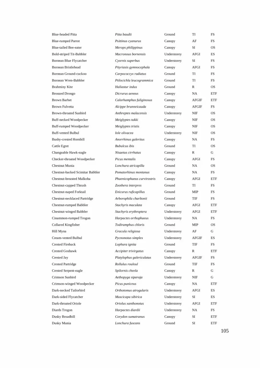
105
Blue-headed Pitta Pitta baudii Ground TI FS
Blue-rumped Parrot Psittinus cyanurus Canopy AF FS
Blue-tailed Bee-eater Merops philippinus Canopy SI OS
Bold-striped Tit-Babbler Macronous bornensis Understorey AFGI ES
Bornean Blue Flycatcher Cyornis superbus Understorey SI FS
Bornean Bristlehead Pityriasis gymnocephala Canopy AFGI FS
Bornean Ground-cuckoo Carpococcyx radiatus Ground TI FS
Bornean Wren-Babbler Ptilocichla leucogrammica Ground TI FS
Brahminy Kite Haliastur indus Ground R OS
Bronzed Drongo Dicrurus aeneus Canopy NA ETF
Brown Barbet Calorhamphus fuliginosus Canopy AFGIF ETF
Brown Fulvetta Alcippe brunneicauda Canopy AFGIF FS
Brown-throated Sunbird Anthreptes malacensis Understorey NIF OS
Buff-necked Woodpecker Meiglyptes tukki Canopy NIF OS
Buff-rumped Woodpecker Meiglyptes tristis Canopy NIF OS
Buff-vented Bulbul Iole olivacea Understorey NIF OS
Bushy-crested Hornbill Anorrhinus galeritus Canopy NA FS
Cattle Egret Bubulcus ibis Ground TI OS
Changeable Hawk-eagle Nisaetus cirrhatus Canopy R G
Checker-throated Woodpecker Picus mentalis Canopy AFGI FS
Chestnut Munia Lonchura atricapilla Ground NA OS
Chestnut-backed Scimitar Babbler Pomatorhinus montanus Canopy NA FS
Chestnut-breasted Malkoha Phaenicophaeus curvirostris Canopy AFGI ETF
Chestnut-capped Thrush Zoothera interpres Ground TI FS
Chestnut-naped Forktail Enicurus ruficapillus Ground MIP FS
Chestnut-necklaced Partridge Arborophila charltonii Ground TIF FS
Chestnut-rumped Babbler Stachyris maculata Canopy AFGI ETF
Chestnut-winged Babbler Stachyris erythroptera Understorey AFGI ETF
Cinammon-rumped Trogon Harpactes orrhophaeus Understorey NA FS
Collared Kingfisher Todiramphus chloris Ground MIP OS
Hill Myna Gracula religiosa Understorey AF G
Cream-vented Bulbul Pycnonotus simplex Understorey AFGIF ES
Crested Fireback Lophura ignita Ground TIF FS
Crested Goshawk Accipiter trivirgatus Canopy R ETF
Crested Jay Platylophus galericulatus Understorey AFGIF FS
Crested Partridge Rollulus rouloul Ground TIF FS
Crested Serpent-eagle Spilornis cheela Canopy R G
Crimson Sunbird Aethopyga siparaja Understorey NIF G
Crimson-winged Woodpecker Picus puniceus Canopy NA ETF
Dark-necked Tailorbird Orthotomus atrogularis Understorey AFGI ES
Dark-sided Flycatcher Muscicapa sibirica Understorey SI ES
Dark-throated Oriole Oriolus xanthonotus Understorey AFGI ETF
Diards Trogon Harpactes diardii Understorey NA FS
Dusky Broadbill Corydon sumatranus Canopy SI ETF
Dusky Munia Lonchura fuscans Ground SI ETF

106
Emerald Dove Chalcophaps indica Ground NA ETF
Ferruginous Babbler Trichastoma bicolor Understorey AFGI FS
Fiery Minivet Pericrocotus igneus Canopy AFGI ETF
Finschs Bulbul Alophoixus finschii Understorey AFGIF ES
Fluffy-backed Tit-babbler Macronous ptilosus Understorey AFGI ETF
Giant Pitta Pitta caerulea Ground TI FS
Golden-whiskered Barbet Megalaima chrysopogon Canopy NA ETF
Great Argus Argusianus argus Ground TIF FS
Great Slaty Woodpecker Mulleripicus pulverulentus Canopy AFGI FS
Greater Coucal Centropus sinensis Ground TI OS
Greater Green Leafbird Chloropsis sonnerati Canopy NIF ETF
Greater Racquet-tailed Drongo Dicrurus paradiseus Canopy NA ETF
Green Broadbill Calyptomena viridis Canopy AF FS
Green Imperial Pigeon Ducula aenea Canopy AF FS
Green Iora Aegithina viridissima Canopy AFGI ETF
Grey-and-buff Woodpecker Hemicircus concretus Canopy AFGI ETF
Grey-bellied Bulbul Pycnonotus cyaniventris Understorey AFGIF ETF
Grey-capped Pygmy Woodpecker Dendrocopos canicapillus Canopy AFGI ETF
Grey-cheeked Bulbul Alophoixus bres Understorey AFGIF FS
Grey-chested Jungle-Flycatcher Rhinomyias umbratilis Understorey NA FS
Grey-headed Babbler Stachyris poliocephala Understorey AFGI FS
Grey-headed Canary-flycatcher Culicicapa ceylonensis Canopy SI ES
Grey-rumped Treeswift Hemiprocne longipennis Canopy NA OS
Hairy-backed Bulbul Tricholestes criniger Understorey AFGIF FS
Helmeted Hornbill Rhinoplax vigil Understorey NA ETF
Hooded Pitta Pitta sordida Ground TI ETF
Horsfields Babbler Malacocincla sepiaria Ground TI ETF
Indian Cuckoo Cuculus micropterus Canopy NA OS
Jerdon's Baza Aviceda jerdoni Understorey R ES
Large Frogmouth Batrachostomus auritus Canopy AFGI FS
Large Green Pigeon Treron capellei Canopy AF ETF
Large Woodshrike Tephrodornis gularis Canopy AFGI ETF
Large-billed Blue Flycatcher Cyornis caerulatus Understorey SI FS
Lesser Coucal Centropus bengalensis Ground TI OS
Lesser Cuckooshrike Coracina fimbriata Canopy AFGI ETF
Lesser Fish-Eagle Ichthyophaga humilis Ground R OS
Lesser Green Leafbird Chloropsis cyanopogon Canopy NIF ETF
Little Bronze Cuckoo Chrysococcyx minutillus Canopy AFGI ETF
Little Egret Egretta garzetta Ground NA OS
Little Green Pigeon Treron olax Canopy AF ETF
Little Spiderhunter Arachnothera longirostra Understorey NIF G
Long-billed Spiderhunter Arachnothera robusta Canopy NA ETF
Long-tailed Parakeet Psittacula longicauda Canopy AF ETF
Malayian Eared-nightjar Eurostopodus temminckii Understorey SI ES
Malaysian Blue Flycatcher Cyornis turcosus Understorey SI ETF

107
Malaysian Hawk-cuckoo Hierococcyx fugax Understorey AFGI ETF
Mangrove Blue Flycatcher Cyornis rufigastra Understorey SI ETF
Maroon Woodpecker Blythipicus rubiginosus Canopy NA ETF
Maroon-breasted Philentoma Philentoma pyrhoptera Understorey SI FS
Moustached Babbler Malacopteron magnirostre Understorey AFGI ETF
Moustached Hawk-cuckoo Hierococcyx vagans Understorey AFGI FS
Narcissus Flycatcher Ficedula narcissina Understorey SI ETF
Olive-backed Pipit Anthus hodgsoni Ground TI ES
Olive-backed Sunbird Nectarinia jugularis Understorey NIF OS
Olive-backed Woodpecker Dinopium rafflesii Canopy NA FS
Olive-winged Bulbul Pycnonotus plumosus Understorey AFGIF ES
Orange-backed Woodpecker Reinwardtipicus validus Canopy NA FS
Orange-bellied Flowerpecker Dicaeum trigonostigma Canopy NIF G
Orange-breasted Trogon Harpactes oreskios Understorey SI FS
Oriental Dollarbird Eurystomus orientalis Canopy SI ES
Oriental Dwarf-kingfisher Ceyx erithaca Understorey NA FS
Oriental Honey Buzzard Pernis ptilorhyncus Canopy R ES
Oriental Magpie-Robin Copsychus saularis Ground AFGI OS
Oriental Pied Hornbill Anthracoceros albirostris Canopy NA OS
Pale Blue Flycatcher Cyornis unicolor Understorey SI FS
Pied Fantail Rhipidura javanica Understorey SI ES
Plain Sunbird Anthreptes simplex Understorey NIF ETF
Plaintive Cuckoo Cacomantis merulinus Understorey AFGI G
Puff-backed Bulbul Pycnonotus eutilotus Understorey AFGIF FS
Purple-naped Sunbird Hypogramma hypogrammicum Understorey NIF ETF
Purple-throated Sunbird Nectarinia sperata Understorey NIF ETF
Raffles's Malkoha Phaenicophaeus chlorophaeus Understorey AFGI ETF
Red-bearded Bee-eater Nyctyornis amictus Canopy SI FS
Red-naped Trogon Harpactes kasumba Understorey NA FS
Red-throated Barbet Megalaima mystacophanos Canopy AFGIF ETF
Red-throated Sunbird Anthreptes rhodolaemus Understorey NIF ES
Rhinoceros Hornbill Buceros rhinoceros Canopy NA ETF
Ruby-cheeked Sunbird Anthreptes singalensis Understorey NIF ES
Rufous Piculet Sasia abnormis Understorey AFGI ETF
Rufous Woodpecker Celeus brachyurus Canopy AFGI ETF
Rufous-bellied Hawk-Eagle Lophotriorchis kienerii Ground R ETF
Rufous-chested Flycatcher Ficedula dumetoria Understorey SI FS
Rufous-crowned Babbler Malacopteron magnum Understorey AFGI FS
Rufous-fronted Babbler Stachyris rufifrons Canopy AFGI ETF
Rufous-tailed Shama Trichixos pyrropygus Ground AFGI FS
Rufous-tailed Tailorbird Orthotomus sericeus Understorey AFGI ES
Rufous-winged Philentoma Philentoma velata Understorey SI FS
Scaly-crowned Babbler Malacopteron cinereum Understorey AFGI FS
Scarlet Minivet Pericrocotus flammeus Canopy AFGI ETF
Scarlet rumped Trogon Harpactes duvaucelii Understorey NA FS

108
Scarlet-breasted Flowerpecker Prionochilus thoracicus Canopy NIF ETF
Short-tailed Babbler Malacocincla malaccensis Ground TI ETF
Short-toed Coucal Centropus rectunguis Ground AFGI FS
Siberian Blue Robin Luscinia cyane Ground TI FS
Slender-billed Crow Corvus enca Ground AFGIF OS
Sooty-capped Babbler Malacopteron affine Understorey AFGI ETF
Spectacled Bulbul Pycnonotus erythropthalmos Understorey AFGIF ETF
Spotted Dove Stigmatopelia chinensis Ground NA OS
Spotted Fantail Rhipidura perlata Understorey SI FS
Square-tailed Drongo-Cuckoo Surniculus lugubris Canopy AFGIF ETF
Storm's Stork Ciconia stormi Ground NA FS
Streaked Bulbul Ixos malaccensis Understorey AFGIF ETF
Streaky-breasted Spiderhunter Arachnothera affinis Understorey NIF FS
Striped Wren-babbler Kenopia striata Ground TI FS
Thick-billed Green Pigeon Treron curvirostra Canopy AF ETF
Thick-billed Spiderhunter Arachnothera crassirostris Canopy NIF ETF
Tree Sparrow Passer montanus Ground NA OS
Velvet-fronted Nuthatch Sitta frontalis Canopy NA FS
Verditer Flycatcher Eumyias thalassinus Canopy SI ETF
Violet Cuckoo Chrysococcyx xanthorhynchus Canopy AFGI ETF
Wallace's Hawk-Eagle Nisaetus nanus Canopy R ETF
Whiskered Treeswift Hemiprocne comata Canopy SI OS
White-bellied Erpornis Erpornis zantholeuca Understorey AFGI FS
White-bellied Munia Lonchura leucogastra Ground TIF OS
White-bellied Woodpecker Dryocopus javensis Canopy AFGI ETF
White-breasted Waterhen Amaurornis phoenicurus Ground MIP OS
White-chested Babbler Trichastoma rostratum Ground TI ES
White-crowned Forktail Enicurus leschenaulti Ground TI FS
White-crowned Hornbill Aceros comatus Canopy NA FS
White-crowned Shama Copsychus stricklandii Understorey AFGI ETF
Wreathed Hornbill Aceros undulatus Canopy NA ETF
Yellow-bellied Bulbul Alophoixus phaeocephalus Understorey AFGIF FS
Yellow-bellied Gerygone Gerygone sulphurea Canopy SI ETF
Yellow-bellied Prinia Prinia flaviventris Understorey AFGI OS
Yellow-breasted Flowerpecker Prionochilus maculatus Canopy AFGIF ETF
Yellow-crowned Barbet Megalaima henricii Canopy AF ETF
Yellow-eared Spiderhunter Arachnothera chrysogenys Canopy NIF FS
Yellow-rumped Flowerpecker Prionochilus xanthopygius Canopy NIF G
Yellow-vented Bulbul Pycnonotus goiavier Understorey AFGIF G

109
Table S 3.2. Details of feeding guild and habitat association codes used in the study.
Trait groups follow Styring (2004) and Sheldon (2010).
AF Arboreal frugivore
AFGI Arboreal foliage-gleaning insectivore
AFGIF Arboreal foliage-gleaning insectivore / frugivore
SI Sallying Insectivore
TI Terrestrial Insectivore
TIF Terrestrial Insectivore / Frugivore
NIF Nectivore / Insectivore / Frugivore
MIP Miscellaneous Insectivore / Pecivore
R Raptor
FS Forest specialist
ETF Edge-tolerant forest
OS Open habitat species
G Generalist
NA Information Not Available / Not assessed

110
Table S 3.3. Median thresholds points with confidence intervals in relation to mean canopy
height and canopy hereogeneity.Canopy heterogenity is stardard deviation of canopy height.
Both metrics calculated from mean LiDAR values within a 50 m radius. Lower 95%
confidence interval; Lw CI, Upper 95% confidence interval; Up CI. Model ΔAIC denotes the
reduction in AIC between linear model and segmented model. Negative ΔAIC signifies that
the linear model out performed the segmented one. G+ denotes whether thresholds were
associated with a strengthing (increasing gradient G+ = True), or weakening (more negative
G+ = False) response after the threshold point.
Species Canopy Height Canopy Heterogeneity
Med Lw
CI
Up
CI
ΔAIC G
+
Med Lw
CI
Up
CI
ΔAIC G
+
Arctic Warbler 28 22 34.3 40.7 F 3 3.6 2.2 69.1 F
Ashy Tailorbird 21.5 14.2 28.5 62.6 F 2.5 6.5 -1.2 -2 F
Asian Fairy Bluebird 33.9 14.4 43.3 101.9 T 3 5.2 1.1 48.6 T
Asian Glossy Starling 33.9 17.9 44.9 39.8 T 5.7 7.8 2.8 28.9 F
Asian Paradise Flycatcher 32.3 16 43.8 9.3 T 3.3 4.9 1.9 13.8 F
Banded Bay Cuckoo 28.9 20.7 37.9 132.1 F 3 4 1.9 52.9 F
Banded Broadbill 33.9 24.6 41.2 35.5 F 2.9 4.2 1.7 31.6 F
Banded Kingfisher 32.3 -40.5 106 78.4 T 3.5 14.7 -7.2 6.3 F
Banded Pitta 29.4 6.1 45.5 112.8 T 3.2 6.3 0.9 8 F
Banded Woodpecker 10 5.7 15.3 53.7 F 3.9 8.6 -0.4 6.4 F
Bar-winged Flycatcher-shrike 26.4 18.4 34 22.7 F 3 3.8 2.1 55.1 F
Black Hornbill 32.1 0.6 59.5 310.6 T 3.6 8.2 -0.2 0.1 F
Black Magpie 32.3 19.4 42.7 58.4 F 2.9 5.3 0.9 27.8 F
Black-and-yellow Broadbill 22.3 5.3 31.9 14.3 T 3.4 6.1 1.1 43.6 T
Black-bellied Malkoha 10.3 5.9 15.6 7.3 T 5.7 10.4 -0.1 -2 F
Black-capped Babbler 32.2 12.6 55.7 195.8 T 3.2 5 1.8 6 F
Black-headed Bulbul 29 12.4 44.2 39.6 T 3.4 6.8 0.6 52.5 T
Black-headed Pitta 26 12 40.3 352.9 F 3 3.9 2 62.2 F
Black-naped Monarch 33.9 10.8 60.8 373.7 T 4.3 6.3 2 0.6 F
Black-winged Flycatcher-shrike 31.2 -3.2 59.8 208.1 T 3.3 5.1 1.7 22 F
Blue-banded Kingfisher 28.8 9.6 41.4 39.6 F 3 5.5 1 44.4 F
Blue-banded Pitta 24.7 13.5 32.2 33.3 F 3 4.1 1.9 61.6 F
Blue-crowned Hanging-parrot 25.4 8.8 45.6 3.8 T 3 4.4 1.8 26.9 F
Blue-eared Barbet 33.8 20 44.1 20.7 T 2.9 4.1 1.7 20.9 F

111
Blue-eared Kingfisher 31.2 18.6 42.8 148.8 F 3.3 7.1 0 6.5 F
Blue-headed Pitta 25.2 7.4 39.4 13.8 F 3 6.2 0.4 -0.6 T
Blue-throated Bee-eater 9.3 5 14.6 14.5 F 4.3 6.1 3 14.9 F
Bold-striped Tit-babbler 34.9 14.3 67.9 723 T 4.4 5.9 2.5 3.1 F
Bornean Blue Flycatcher 22.5 8.7 31.5 62.6 F 3.4 6.1 1.3 29 F
Bornean Bristlehead 27.3 16.5 36.9 61 F 3.1 4.6 1.8 76.5 F
Bornean Ground-cuckoo 35 4.7 62 58 T 3.2 7.3 -0.3 50.5 T
Bornean Wren-babbler 15.3 3.2 35.4 157.6 T 3.4 6 0.9 343 T
Bronzed Drongo 23.4 16.3 30.7 88.5 F 3.4 5.6 1.3 173 F
Brown Barbet 29 8.8 41.5 67.8 T 3.1 6.7 0.5 19.1 T
Brown Flycatcher 34.6 18.7 57.8 38.7 T 3 5 1.3 5.5 F
Brown Fulvetta 11.4 4.6 31.2 109.7 F 3.2 5.6 1 106 F
Brown-throated Sunbird 31.9 5.4 51.4 205.2 T 3.2 5.6 1.5 5.2 F
Buff-rumped Woodpecker 35.2 21.4 53.5 78.1 T 3 4.2 1.9 10 F
Buff-vented Bulbul 22.9 6.7 32.3 58.4 F 3.2 5.2 1.4 176 F
Bushy-crested Hornbill 34 18.2 47.2 14 T 3 5.2 0.7 21.6 T
Checker-throated Woodpecker 22.7 11.4 31.9 17.4 T 3.1 4.5 1.7 77.3 T
Chestnut Munia 22.9 8.5 33.5 16.6 T 2.7 4.7 0.9 38 T
Chestnut-backed Scimitar-babbler 33.9 19 45.9 130.6 T 2.8 3.9 1.8 36.5 T
Chestnut-breasted Malkoha 27.9 6.3 42.2 32.8 F 3.3 6.6 0.5 81.1 F
Chestnut-naped Forktail 32.3 0.9 56.5 54.6 T 3.4 11.1 -3 14.3 T
Chestnut-necklaced Partridge 20.2 7.9 26 53.4 F 3.2 4.6 2.1 63.8 F
Chestnut-rumped Babbler 26.1 6.9 41.8 23.1 F 3.2 5.4 1.4 77.5 F
Chestnut-winged Babbler 35.2 8.2 70.9 346 T 4.4 6.7 1.7 3.5 F
Collared Kingfisher 31.7 16 45.7 55.9 T 3 4.4 1.7 10.3 F
Cream-vented Bulbul 24.6 4.8 41.6 154.6 T 3.8 6.3 1.4 244 T
Crested Fireback 29.1 17.2 40.4 48.1 T 3.2 5 1.6 111 T
Crested Goshawk 21.4 0.7 44.3 -3.3 T 3.3 7.1 0 131 F
Crested Jay 34 26 40 34.7 F 3 3.9 2 37.3 F
Crested Serpent-eagle 11.2 6.9 20.7 155.4 F 3.3 5 1.8 304 F
Crimson Sunbird 25.2 17.6 32 22.3 F 3 4 2.2 41.1 F
Crimson-winged Woodpecker 25.6 12 37.5 0.5 T 3 4.4 1.8 26.2 F
Dark-necked Tailorbird 33.9 18.6 42.9 41.7 F 3 5.4 0.9 16 F
Dark-sided Flycatcher 31.2 13.1 42.5 206.4 F 3.2 6.1 1.2 71.4 F
Dark-throated Oriole 33.9 21.6 42.7 4.7 F 3 4.1 1.8 30.2 F
Diards Trogon 31.5 19 42.9 14.3 F 2.9 4.2 1.6 33.9 F
Drongo Cuckoo 25.6 20.3 32.7 64.3 F 3 4.2 2 81 F
Dusky Broadbill 9.8 4.7 14.7 197.9 F 3.4 4.7 2.1 295 F
Dusky Munia 25.3 15.5 34.5 52.6 F 3 3.7 2.2 45.6 F
Emerald Dove 28.2 20.1 35.6 44.8 T 3.2 4.5 2 90 T
Ferruginous Babbler 25.5 15.1 33.8 58.2 F 3.1 4.3 1.9 122 F
Fiery Minivet 21.2 10.1 27.8 49.7 F 3.2 4.2 2.2 111 F
Finschs Bulbul 26.6 18.8 34.3 95.2 T 2.8 3.7 2 56.8 T
Fluffy-backed Tit-babbler 9.9 8.1 19.1 12.8 F 3.2 4.2 2.3 40.6 F
Golden-bellied Gerygone 26.5 8.5 40.6 34 T 3.1 4.4 2.1 24.9 F

112
Gold-whiskered Barbet 31.5 8.2 53.5 239.5 T 3.6 7.6 0.1 -2.5 F
Great Argus 27.3 5.3 50.8 95.3 T 3 7.6 -0.6 -1.6 F
Great Slaty Woodpecker 24.6 13.8 33.3 96.3 F 3.7 6.3 1.1 220 F
Greater Coucal 34 17.7 52.2 199.4 T 3 4.4 1.8 5.1 F
Greater Green Leafbird 25.3 7.4 36.6 61.9 F 3.2 6.6 0.9 12.3 F
Greater Racket-tailed Drongo 28.7 15.5 39.9 11.5 T 2.8 4.1 1.6 38.4 T
Green Broadbill 34 21.2 46.9 57.7 T 3 4.4 1.5 8.7 F
Green Imperial Pigeon 33.9 20 44.6 34.5 T 3 4.2 1.7 15.1 F
Green Iora 25.4 19 32.2 88.7 F 3.2 4.6 1.8 130 F
Grey Wagtail 25.6 18.3 37.2 12.2 F 3 4 2 29.7 F
Grey-and-buff Woodpecker 10.2 6.1 17.8 61.2 F 3.2 4.8 1.8 209 F
Grey-bellied Bulbul 25.3 14.5 35.2 67.7 T 3.2 4.2 2.2 143 T
Grey-cheeked Bulbul 25.3 7 36 11.3 T 3.1 5.9 1 -3.4 T
Grey-chested Jungle-flycatcher 34.7 23.8 50.6 35.6 T 3.1 4.3 2 7.6 F
Grey-headed Babbler 31.7 10.3 48.4 44.6 F 3 7.1 -0.7 19.1 F
Grey-headed Canary-flycatcher 25.6 12.2 34.4 29.8 F 3 3.8 1.9 77.8 F
Grey-rumped Treeswift 32.5 9.6 47.4 213.1 T 3.3 5.5 1.6 6.1 F
Hairy-backed Bulbul 25.4 7.3 41.4 26.9 T 3 4.1 2.1 16.1 F
Helmeted Hornbill 25 4.3 41.5 621.6 T 3 5.4 1.1 48 T
Hill Myna 25.3 10 35.2 11.9 F 3.1 5.4 1.2 35 F
Hooded Pitta 34.1 25.1 41.4 62.5 F 3 4.2 1.8 36.7 F
Horsfields Babbler 21.7 7.3 33.2 10.5 F 3.8 8.1 0.5 12 F
Large Green Pigeon 25.3 4.6 39.1 207.8 T 3.6 5.9 1.4 241 T
Large Woodshrike 35.5 19 66.2 232.1 T 4.4 6.8 1.9 -1.1 F
Lesser Coucal 21 6.4 30.8 44.6 F 3.4 5.5 1.9 179 F
Lesser Green Leafbird 34 15.5 44.3 18.7 F 5.4 7.2 2.8 71.2 F
Little Egret 28.8 21.2 36 81.5 F 3 3.9 2.1 79.5 F
Little Green Pigeon 35.6 16.6 68 332.3 T 4.4 6.2 1.9 2.5 F
Little Spiderhunter 26.5 14.5 37.7 129.1 F 3 4.1 1.9 56.1 F
Long-billed Spiderhunter 31.5 8.2 43.6 8.6 T 4.2 6.6 1.7 16.5 F
Long-tailed Parakeet 28 21.8 35 63.3 F 3 3.8 2.1 62.1 F
Malaysian Blue Flycatcher 34.4 25.8 41.7 14.4 F 3 3.8 2.1 35.6 F
Maroon Woodpecker 14 5.3 31.6 151.6 F 3.1 4.8 1.6 193 F
Maroon-breasted Philentoma 33.9 10 56.5 97.5 T 4.4 11.6 -1.3 -3.1 F
Moustached Babbler 25.3 15.4 35.4 18.8 F 3 4.1 2 62.1 F
Olive-backed Woodpecker 10.3 4.4 19.9 244.4 T 3.5 5.3 1.8 294 T
Olive-winged Bulbul 25.4 16.2 33 131.7 F 3.2 4.5 1.9 116 F
Orange-backed Woodpecker 25 9.2 34.3 2.2 F 3 4.3 1.8 56.1 F
Orange-bellied Flowerpecker 34.2 20.5 47.4 7.7 T 3 4.6 1.7 14.7 F
Oriental Dwarf Kingfisher 31.8 11.5 45.7 37.5 T 4.4 6.5 2.2 13.1 F
Oriental Honey Buzzard 29.3 -0.2 51.3 16.9 F 3.6 10.3 -1.5 4.2 T
Oriental Magpie Robin 28.5 13.2 42.3 1.9 F 3 4.7 1.6 34.4 F
Pied Fantail 31.1 10.9 45.4 311.4 F 3.2 5.6 1.8 13.7 T
Plain Sunbird 25.4 20.4 31.9 34.6 F 3 3.7 2.2 52.2 F
Plaintive Cuckoo 34.2 27.2 40.9 8.7 F 2.9 3.9 2 22.9 F
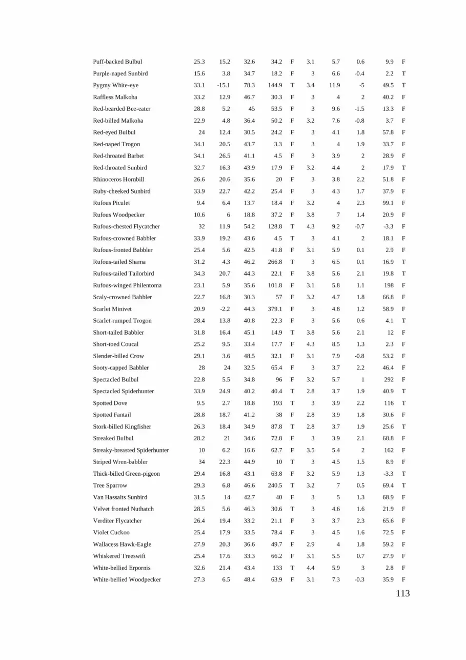
113
Puff-backed Bulbul 25.3 15.2 32.6 34.2 F 3.1 5.7 0.6 9.9 F
Purple-naped Sunbird 15.6 3.8 34.7 18.2 F 3 6.6 -0.4 2.2 T
Pygmy White-eye 33.1 -15.1 78.3 144.9 T 3.4 11.9 -5 49.5 T
Raffless Malkoha 33.2 12.9 46.7 30.3 F 3 4 2 40.2 F
Red-bearded Bee-eater 28.8 5.2 45 53.5 F 3 9.6 -1.5 13.3 F
Red-billed Malkoha 22.9 4.8 36.4 50.2 F 3.2 7.6 -0.8 3.7 F
Red-eyed Bulbul 24 12.4 30.5 24.2 F 3 4.1 1.8 57.8 F
Red-naped Trogon 34.1 20.5 43.7 3.3 F 3 4 1.9 33.7 F
Red-throated Barbet 34.1 26.5 41.1 4.5 F 3 3.9 2 28.9 F
Red-throated Sunbird 32.7 16.3 43.9 17.9 F 3.2 4.4 2 17.9 T
Rhinoceros Hornbill 26.6 20.6 35.6 20 F 3 3.8 2.2 51.8 F
Ruby-cheeked Sunbird 33.9 22.7 42.2 25.4 F 3 4.3 1.7 37.9 F
Rufous Piculet 9.4 6.4 13.7 18.4 F 3.2 4 2.3 99.1 F
Rufous Woodpecker 10.6 6 18.8 37.2 F 3.8 7 1.4 20.9 F
Rufous-chested Flycatcher 32 11.9 54.2 128.8 T 4.3 9.2 -0.7 -3.3 F
Rufous-crowned Babbler 33.9 19.2 43.6 4.5 T 3 4.1 2 18.1 F
Rufous-fronted Babbler 25.4 5.6 42.5 41.8 F 3.1 5.9 0.1 2.9 F
Rufous-tailed Shama 31.2 4.3 46.2 266.8 T 3 6.5 0.1 16.9 T
Rufous-tailed Tailorbird 34.3 20.7 44.3 22.1 F 3.8 5.6 2.1 19.8 T
Rufous-winged Philentoma 23.1 5.9 35.6 101.8 F 3.1 5.8 1.1 198 F
Scaly-crowned Babbler 22.7 16.8 30.3 57 F 3.2 4.7 1.8 66.8 F
Scarlet Minivet 20.9 -2.2 44.3 379.1 F 3 4.8 1.2 58.9 F
Scarlet-rumped Trogon 28.4 13.8 40.8 22.3 F 3 5.6 0.6 4.1 T
Short-tailed Babbler 31.8 16.4 45.1 14.9 T 3.8 5.6 2.1 12 F
Short-toed Coucal 25.2 9.5 33.4 17.7 F 4.3 8.5 1.3 2.3 F
Slender-billed Crow 29.1 3.6 48.5 32.1 F 3.1 7.9 -0.8 53.2 F
Sooty-capped Babbler 28 24 32.5 65.4 F 3 3.7 2.2 46.4 F
Spectacled Bulbul 22.8 5.5 34.8 96 F 3.2 5.7 1 292 F
Spectacled Spiderhunter 33.9 24.9 40.2 40.4 T 2.8 3.7 1.9 40.9 T
Spotted Dove 9.5 2.7 18.8 193 T 3 3.9 2.2 116 T
Spotted Fantail 28.8 18.7 41.2 38 F 2.8 3.9 1.8 30.6 F
Stork-billed Kingfisher 26.3 18.4 34.9 87.8 T 2.8 3.7 1.9 25.6 T
Streaked Bulbul 28.2 21 34.6 72.8 F 3 3.9 2.1 68.8 F
Streaky-breasted Spiderhunter 10 6.2 16.6 62.7 F 3.5 5.4 2 162 F
Striped Wren-babbler 34 22.3 44.9 10 T 3 4.5 1.5 8.9 F
Thick-billed Green-pigeon 29.4 16.8 43.1 63.8 F 3.2 5.9 1.3 -3.3 T
Tree Sparrow 29.3 6.8 46.6 240.5 T 3.2 7 0.5 69.4 T
Van Hassalts Sunbird 31.5 14 42.7 40 F 3 5 1.3 68.9 F
Velvet fronted Nuthatch 28.5 5.6 46.3 30.6 T 3 4.6 1.6 21.9 F
Verditer Flycatcher 26.4 19.4 33.2 21.1 F 3 3.7 2.3 65.6 F
Violet Cuckoo 25.4 17.9 33.5 78.4 F 3 4.5 1.6 72.5 F
Wallacess Hawk-Eagle 27.9 20.3 36.6 49.7 F 2.9 4 1.8 59.2 F
Whiskered Treeswift 25.4 17.6 33.3 66.2 F 3.1 5.5 0.7 27.9 F
White-bellied Erpornis 32.6 21.4 43.4 133 T 4.4 5.9 3 2.8 F
White-bellied Woodpecker 27.3 6.5 48.4 63.9 F 3.1 7.3 -0.3 35.9 F

114
White-chested Babbler 28.1 22 36.1 48.1 F 2.9 3.8 2 47.9 F
White-crowned Forktail 25.3 18.7 33.6 44.9 F 3 4.2 1.7 37.4 F
White-crowned Shama 21.9 8.1 31.8 38.5 F 3 4 2.1 105 F
Wreathed Hornbill 34 18.1 60.5 701.5 T 3.5 5.7 2.1 2.7 F
Yellow-bellied Bulbul 25.6 13 40 26.3 F 3 4.7 1.2 36.3 F
Yellow-bellied Prinia 31.5 10.4 45.7 53.6 F 2.9 4.3 1.5 13.2 F
Yellow-breasted Flowerpecker 33.9 13.3 46.7 145.6 T 3.3 4.8 1.9 117 T
Yellow-crowned Barbet 26 10.8 38.1 1.6 F 3.2 6.6 0.9 3.4 F
Yellow-eared Spiderhunter 15.9 6.6 28.7 89.5 F 3.3 5.1 1.7 252 F
Yellow-rumped Flowerpecker 32.3 21.2 39.8 36.9 F 3 5.5 0.7 13.3 F
Yellow-vented Bulbul 25.5 16 32.7 35.3 F 3 3.7 2.2 72.1 F
Yellow-vented Flowerpecker 34 21.6 41 53.7 F 3 3.8 2.1 50 F
Zebra Dove 31.6 14.1 47.4 10.8 T 3.2 4.7 2.2 14 F
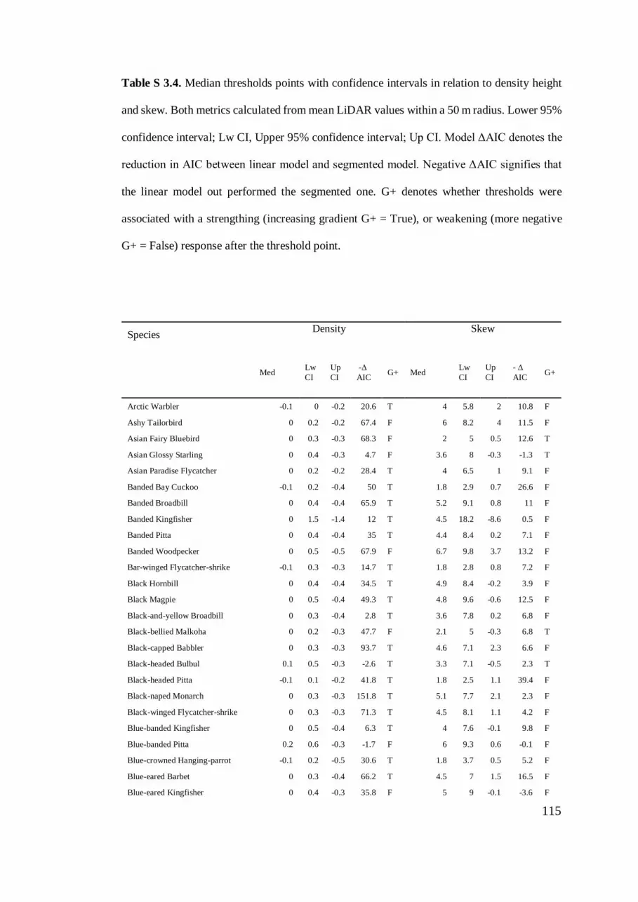
115
Table S 3.4. Median thresholds points with confidence intervals in relation to density height
and skew. Both metrics calculated from mean LiDAR values within a 50 m radius. Lower 95%
confidence interval; Lw CI, Upper 95% confidence interval; Up CI. Model ΔAIC denotes the
reduction in AIC between linear model and segmented model. Negative ΔAIC signifies that
the linear model out performed the segmented one. G+ denotes whether thresholds were
associated with a strengthing (increasing gradient G+ = True), or weakening (more negative
G+ = False) response after the threshold point.
Species Density
Skew
Med Lw
CI
Up
CI
-Δ
AIC G+ Med
Lw
CI
Up
CI
- Δ
AIC G+
Arctic Warbler -0.1 0 -0.2 20.6 T 4 5.8 2 10.8 F
Ashy Tailorbird 0 0.2 -0.2 67.4 F 6 8.2 4 11.5 F
Asian Fairy Bluebird 0 0.3 -0.3 68.3 F 2 5 0.5 12.6 T
Asian Glossy Starling 0 0.4 -0.3 4.7 F 3.6 8 -0.3 -1.3 T
Asian Paradise Flycatcher 0 0.2 -0.2 28.4 T 4 6.5 1 9.1 F
Banded Bay Cuckoo -0.1 0.2 -0.4 50 T 1.8 2.9 0.7 26.6 F
Banded Broadbill 0 0.4 -0.4 65.9 T 5.2 9.1 0.8 11 F
Banded Kingfisher 0 1.5 -1.4 12 T 4.5 18.2 -8.6 0.5 F
Banded Pitta 0 0.4 -0.4 35 T 4.4 8.4 0.2 7.1 F
Banded Woodpecker 0 0.5 -0.5 67.9 F 6.7 9.8 3.7 13.2 F
Bar-winged Flycatcher-shrike -0.1 0.3 -0.3 14.7 T 1.8 2.8 0.8 7.2 F
Black Hornbill 0 0.4 -0.4 34.5 T 4.9 8.4 -0.2 3.9 F
Black Magpie 0 0.5 -0.4 49.3 T 4.8 9.6 -0.6 12.5 F
Black-and-yellow Broadbill 0 0.3 -0.4 2.8 T 3.6 7.8 0.2 6.8 F
Black-bellied Malkoha 0 0.2 -0.3 47.7 F 2.1 5 -0.3 6.8 T
Black-capped Babbler 0 0.3 -0.3 93.7 T 4.6 7.1 2.3 6.6 F
Black-headed Bulbul 0.1 0.5 -0.3 -2.6 T 3.3 7.1 -0.5 2.3 T
Black-headed Pitta -0.1 0.1 -0.2 41.8 T 1.8 2.5 1.1 39.4 F
Black-naped Monarch 0 0.3 -0.3 151.8 T 5.1 7.7 2.1 2.3 F
Black-winged Flycatcher-shrike 0 0.3 -0.3 71.3 T 4.5 8.1 1.1 4.2 F
Blue-banded Kingfisher 0 0.5 -0.4 6.3 T 4 7.6 -0.1 9.8 F
Blue-banded Pitta 0.2 0.6 -0.3 -1.7 F 6 9.3 0.6 -0.1 F
Blue-crowned Hanging-parrot -0.1 0.2 -0.5 30.6 T 1.8 3.7 0.5 5.2 F
Blue-eared Barbet 0 0.3 -0.4 66.2 T 4.5 7 1.5 16.5 F
Blue-eared Kingfisher 0 0.4 -0.3 35.8 F 5 9 -0.1 -3.6 F

116
Blue-headed Pitta 0 0.3 -0.3 61.5 F 5.6 8.9 1 19.9 T
Blue-throated Bee-eater 0 0.4 -0.3 18.1 F 6.7 10.4 2.4 169.1 T
Bold-striped Tit-babbler 0 0.2 -0.2 50.9 T 4.5 6.8 2.4 -0.1 F
Bornean Blue Flycatcher 0 0.3 -0.3 32.2 F 5.5 9.1 0.7 2.3 F
Bornean Bristlehead -0.1 0.3 -0.3 8.5 T 2.1 5.9 0.4 7.8 F
Bornean Ground-cuckoo 0.1 0.6 -0.5 2.9 F 2.3 6.9 -1.4 0.2 T
Bornean Wren-babbler 0.1 0.4 -0.3 -0.8 F 1.8 4.5 -0.5 75.8 T
Bronzed Drongo -0.1 0.2 -0.3 11.6 F 7.2 11.2 2.9 114 F
Brown Barbet 0 0.4 -0.4 78.2 F 3.6 8.5 -0.1 6.4 T
Brown Flycatcher -0.1 0.3 -0.5 4.4 T 4.3 9.7 1.1 -1.9 F
Brown Fulvetta 0 0.3 -0.2 2.6 T 1.9 3.5 0.5 54.5 F
Brown-throated Sunbird 0 0.4 -0.3 91.2 T 4.6 7.6 1 7.1 F
Buff-rumped Woodpecker -0.1 0.2 -0.4 28.2 T 4.1 6.6 1.5 1.4 F
Buff-vented Bulbul 0 0.3 -0.3 -1.9 T 1.9 3.5 0.2 50 F
Bushy-crested Hornbill 0 0.6 -0.6 68.1 F 4.5 10.5 -1.1 4 T
Checker-throated Woodpecker 0.4 0.6 0.2 -1.4 F 3.4 7.4 -0.6 4.9 T
Chestnut Munia 0 0.4 -0.3 1.4 F 2.6 6.4 -0.8 1.7 T
Chestnut-backed Scimitar-babbler 0 0.2 -0.2 60.4 F 5.4 8 1.6 28.4 T
Chestnut-breasted Malkoha 0 0.4 -0.4 43.1 F 2.2 5.9 0 32.6 F
Chestnut-naped Forktail 0 0.7 -0.6 31 F 3.9 11.1 -2.8 5.2 T
Chestnut-necklaced Partridge -0.1 0 -0.3 13 F 7.1 9.8 3.8 22.9 F
Chestnut-rumped Babbler 0 0.3 -0.4 12.6 T 2.1 4.8 0.2 19.1 F
Chestnut-winged Babbler 0 0.4 -0.3 31.3 T 4.4 8.1 1.1 -1.3 F
Collared Kingfisher 0 0.3 -0.3 63.5 T 4.4 6.9 1.1 12.5 F
Cream-vented Bulbul 0.1 0.4 -0.3 -0.3 F 1.6 3.5 -0.3 75.7 T
Crested Fireback 0.1 0.5 -0.2 -0.5 F 3.4 5.7 0.2 18.2 T
Crested Goshawk 0.2 0.7 -0.4 25.3 T 3.4 8.9 -1.6 2.2 F
Crested Jay -0.1 0.3 -0.5 40.6 T 3.9 6.7 1.1 7.8 F
Crested Serpent-eagle 0.1 0.3 -0.2 -0.9 T 6.5 8.5 0.9 92.8 F
Crimson Sunbird 0.2 0.5 -0.2 -2.7 F 6.3 8.9 2.7 -0.2 T
Crimson-winged Woodpecker -0.1 0.3 -0.4 18.4 T 3.6 6.5 0.4 2.4 F
Dark-necked Tailorbird 0 0.3 -0.3 373.7 T 6.2 9.9 0.9 -2.2 F
Dark-sided Flycatcher 0 0.4 -0.3 21 T 2.1 5.1 0.5 24.2 F
Dark-throated Oriole -0.1 0.3 -0.5 26.4 T 4 8 0.7 5.7 F
Diards Trogon 0 0.3 -0.3 69.4 T 4.6 7.6 0.9 26.1 F
Drongo Cuckoo -0.1 0 -0.2 0.8 F 6.1 9.1 1 6.1 F
Dusky Broadbill 0.1 0.3 -0.1 NA F 1.7 2.7 0.5 71.2 F
Dusky Munia -0.2 0.1 -0.4 58.8 T 4 6 1.6 15.9 F
Emerald Dove -0.1 0.1 -0.2 -2.4 F 3.2 5.7 0.4 5.7 T
Ferruginous Babbler 0 0.4 -0.3 2.7 T 1.9 3.6 0.4 20 F
Fiery Minivet -0.1 0 -0.3 -0.9 F 1.2 2.8 0.4 19.5 F
Finschs Bulbul -0.1 0 -0.2 58.2 F 4 6 1.2 24.6 T
Fluffy-backed Tit-babbler -0.1 0.3 -0.3 3.2 F 6.6 9.6 2.8 4 T
Golden-bellied Gerygone -0.1 0.2 -0.4 23.9 T 3.8 6.6 0.6 -0.7 F
Gold-whiskered Barbet 0 0.3 -0.3 86.6 T 5.3 8.7 0.9 3.5 F

117
Great Argus 0 0.3 -0.4 54.1 T 5.5 8.5 0.8 -1 F
Great Slaty Woodpecker -0.1 0.2 -0.3 0.6 F 6.8 12.5 0.1 142 F
Greater Coucal 0 0.2 -0.3 52.6 T 4.4 6.7 2 5.2 F
Greater Green Leafbird 0 0.4 -0.4 46.1 F 3.8 7.7 0.1 -1.9 T
Greater Racket-tailed Drongo 0 0.3 -0.3 53.6 F 4.5 7.5 0.7 23.7 T
Green Broadbill -0.1 0.3 -0.4 18.5 T 4.2 7.3 1.2 3.3 F
Green Imperial Pigeon -0.1 0.2 -0.4 38.7 T 4.2 6.8 1.4 6.5 F
Green Iora -0.1 0.1 -0.3 NA F 3.8 7.1 0.3 25 F
Grey Wagtail -0.1 0.2 -0.5 0.6 T 7.3 10.2 3.1 -2.8 F
Grey-and-buff Woodpecker 0.1 0.3 -0.3 -1.2 T 1.7 3.2 0.3 57.8 F
Grey-bellied Bulbul -0.1 0 -0.2 3.9 F 1.1 2.1 0.4 25.1 T
Grey-cheeked Bulbul -0.1 0.2 -0.3 51.8 F 2.1 5.5 0.5 5.2 T
Grey-chested Jungle-flycatcher -0.1 0.2 -0.4 18.1 T 4 6.6 1 0 F
Grey-headed Babbler 0 0.7 -0.7 28.1 T 4.3 11.2 -1.3 14.6 F
Grey-headed Canary-flycatcher -0.1 0.2 -0.3 8.3 T 1.7 2.7 0.7 14 F
Grey-rumped Treeswift 0 0.2 -0.2 62.2 T 4.4 7.4 1 10.9 F
Hairy-backed Bulbul -0.1 0.2 -0.3 42.4 T 4 6.3 1 10.4 F
Helmeted Hornbill 0 0.2 -0.3 32.1 F 2 3.5 0.7 36.9 T
Hill Myna 0 0.3 -0.3 1.2 F 5.8 9 0.6 -0.5 T
Hooded Pitta -0.1 0.2 -0.5 62.1 T 1.9 3.6 0.7 6.8 F
Horsfields Babbler 0 0.3 -0.4 17.8 F 6.4 10.2 0.2 12 F
Large Green Pigeon 0.1 0.4 -0.3 -0.5 F 1.8 3.8 0.1 33.5 T
Large Woodshrike 0 0.3 -0.3 16.6 T 4.4 7.9 0.9 -2.5 F
Lesser Coucal 0.1 0.5 -0.3 -1.2 F 3.6 7.1 0 93.5 F
Lesser Green Leafbird 0 0.3 -0.3 9.3 F 1.4 3.1 0.1 24.8 F
Little Egret -0.1 0 -0.3 24.3 T 1.7 2.5 0.5 18.8 F
Little Green Pigeon 0 0.2 -0.3 21.4 T 4.4 7.2 1.5 -1.7 F
Little Spiderhunter -0.1 0.2 -0.3 46.3 T 1.9 2.8 0.9 26.5 F
Long-billed Spiderhunter 0 0.5 -0.4 4.4 F 4.2 9.1 0.1 46.7 T
Long-tailed Parakeet -0.1 0 -0.3 43 T 1.8 2.8 0.7 18.4 F
Malaysian Blue Flycatcher -0.1 0.2 -0.5 29.9 T 3.8 7.4 1 4 F
Maroon Woodpecker 0 0.3 -0.2 2.6 T 1.9 3.1 0.4 61 F
Maroon-breasted Philentoma 0 0.4 -0.3 31.9 T 3.2 8.4 -0.7 -1.9 F
Moustached Babbler -0.1 0.2 -0.4 10.4 T 1.8 3.3 0.7 2.1 F
Olive-backed Woodpecker 0.1 0.3 -0.2 0 F 1.7 3.3 0.1 33.3 T
Olive-winged Bulbul -0.1 0 -0.2 0.9 T 5.7 9.2 0.7 22.5 F
Orange-backed Woodpecker 0.2 0.6 -0.3 -0.1 T 3.8 7 0.3 -0.6 F
Orange-bellied Flowerpecker -0.1 0.2 -0.4 11.8 T 4.4 8.5 1.9 0.4 F
Oriental Dwarf Kingfisher 0 0.3 -0.4 0.3 T 4.3 7.4 0.6 1.5 T
Oriental Honey Buzzard 0 0.6 -0.5 23.9 F 3.3 9.2 -2.8 1.1 T
Oriental Magpie Robin -0.1 0.3 -0.4 24.2 T 3.6 6.7 0.5 4.4 F
Pied Fantail 0 0.2 -0.2 60.9 F 5.2 7.5 1.9 12.8 T
Plain Sunbird -0.1 0.2 -0.5 33.1 T 1.8 4.1 0.6 7.4 F
Plaintive Cuckoo -0.1 0.2 -0.4 29.3 T 4 6.9 1.6 7.2 F
Puff-backed Bulbul 0 0.3 -0.3 8.4 T 4.8 9.2 0.1 10.2 T

118
Purple-naped Sunbird 0 0.2 -0.3 73 F 1.9 4 0.5 4.1 T
Pygmy White-eye 0 1 -0.9 9.9 F 2.2 10.3 -5.5 6.1 T
Raffless Malkoha -0.2 0.1 -0.4 72.8 T 4 6 1 14.8 F
Red-bearded Bee-eater 0 0.8 -0.7 8.8 T 4.5 11.2 -3.3 8.6 F
Red-billed Malkoha 0 0.6 -0.5 38.6 F 6.2 11.2 -1.6 18.5 T
Red-eyed Bulbul 0 0.4 -0.2 -2.6 T 3.9 7.2 0.5 1.7 F
Red-naped Trogon -0.1 0.3 -0.5 20.9 T 4 7.4 0.5 2.3 F
Red-throated Barbet -0.1 0.3 -0.5 61.4 T 4 6.2 1.9 12.2 F
Red-throated Sunbird 0 0.2 -0.2 37.8 F 4.4 7 1.7 8.5 T
Rhinoceros Hornbill -0.1 0.2 -0.5 24.4 T 3.9 6.2 1 3.2 F
Ruby-cheeked Sunbird -0.1 0.3 -0.5 51.9 T 4 8.1 0.6 11.5 F
Rufous Piculet -0.1 0.1 -0.3 0.4 T 1.1 2.1 0.2 12.5 F
Rufous Woodpecker 0 0.4 -0.4 37.3 F 6.6 9.9 3.2 21 F
Rufous-chested Flycatcher 0 0.4 -0.3 64.3 T 5.5 9.8 -0.3 -2 F
Rufous-crowned Babbler -0.1 0.2 -0.4 17.5 T 4.2 7.4 1.9 0.3 F
Rufous-fronted Babbler 0 0.4 -0.4 38.2 F 3.1 8.2 -0.1 33.8 T
Rufous-tailed Shama 0 0.2 -0.3 41.9 F 2 3.4 0.7 28.2 T
Rufous-tailed Tailorbird 0 0.2 -0.2 22.6 F 5.1 7.5 1.4 7.4 T
Rufous-winged Philentoma 0 0.3 -0.3 -1.8 T 3 7.6 0.3 48 F
Scaly-crowned Babbler -0.1 0.1 -0.3 16.8 F 6.7 10.1 3.1 12.1 F
Scarlet Minivet 0 0.2 -0.2 30.9 T 1.9 3 0.7 37.3 F
Scarlet-rumped Trogon 0 0.2 -0.2 40.8 F 5.4 7.9 1.3 18.3 T
Short-tailed Babbler -0.1 0.2 -0.4 0.5 T 4.1 7.8 1.1 -3.5 T
Short-toed Coucal 0 0.4 -0.3 54.1 F 4 8.5 0.2 2.6 T
Slender-billed Crow 0 0.7 -0.6 23.6 T 4.4 12.2 -2.2 14.3 F
Sooty-capped Babbler -0.1 0 -0.3 56.5 T 3.8 5.6 1.2 16.1 F
Spectacled Bulbul 0.1 0.4 -0.3 -1.4 T 2.2 6.3 -0.5 93.4 F
Spectacled Spiderhunter -0.1 0.2 -0.3 67.3 F 4.5 6.5 2.2 24.8 T
Spotted Dove -0.1 0.2 -0.2 17.9 F 1.7 2.6 0.9 36.5 T
Spotted Fantail 0 0.2 -0.2 58.1 T 4.6 7.1 2.1 23.9 F
Stork-billed Kingfisher -0.2 0.1 -0.4 66.7 F 4.5 6.4 3.1 22.7 T
Streaked Bulbul -0.1 0 -0.3 16.5 T 1.7 2.8 0.6 15.6 F
Streaky-breasted Spiderhunter 0.1 0.4 -0.3 -0.1 F 1.7 3.7 0.1 67.6 F
Striped Wren-babbler -0.1 0.2 -0.5 13.6 T 4 6.8 1.2 3.4 F
Thick-billed Green-pigeon 0 0.2 -0.2 67.7 F 5.8 8.6 1.7 10.1 T
Tree Sparrow 0 0.4 -0.4 52 F 2.5 8.4 -0.4 22.4 T
Van Hassalts Sunbird 0 0.4 -0.4 14.9 T 4.7 9.3 0.3 7 F
Velvet fronted Nuthatch -0.1 0.2 -0.4 43.4 T 1.9 3.8 0.8 9.4 F
Verditer Flycatcher -0.1 0.2 -0.3 9.3 T 3.4 5.6 0.6 1.5 F
Violet Cuckoo -0.1 0.2 -0.3 -1.2 F 6.7 11.3 2 7.3 F
Wallacess Hawk-Eagle 0 0.6 -0.4 21 T 3.7 6.1 0.1 10.6 F
Whiskered Treeswift -0.1 0.4 -0.6 10.9 F 6.7 10 3.5 4.9 F
White-bellied Erpornis 0 0.1 -0.2 22.9 T 4.4 6.7 1.7 -3.3 T
White-bellied Woodpecker 0 0.5 -0.5 22.9 T 4.5 10 -0.8 2 F
White-chested Babbler -0.1 0.3 -0.4 45 T 1.8 3.3 0.7 17.8 F

119
White-crowned Forktail 0 0.3 -0.3 39.5 T 6.3 9.8 2.5 -0.7 F
White-crowned Shama -0.1 0.1 -0.3 2.8 T 1.1 2.2 0.3 20.6 F
Wreathed Hornbill 0 0.2 -0.2 58.5 T 4.5 6.7 2.4 1.8 F
Yellow-bellied Bulbul 0.2 0.7 -0.5 2.7 T 6.5 12.1 -0.2 0.1 F
Yellow-bellied Prinia 0 0.1 -0.2 54.7 T 5.4 7.7 2.4 22.3 F
Yellow-breasted Flowerpecker -0.1 0 -0.3 12.9 F 1.2 2.5 0.5 13.9 T
Yellow-crowned Barbet 0 0.4 -0.3 72.3 F 5.1 8.9 0.4 8 F
Yellow-eared Spiderhunter 0.1 0.3 -0.3 -0.8 T 3.1 6 0.4 99.8 F
Yellow-rumped Flowerpecker 0 0.3 -0.3 414.9 T 6.4 10.2 2.1 -1.7 F
Yellow-vented Bulbul -0.1 0.1 -0.3 17.1 T 1.2 2.6 0.7 11.3 F
Yellow-vented Flowerpecker -0.1 0.1 -0.4 76.3 T 3.8 5.9 1 17.5 F
Zebra Dove -0.1 0.2 -0.4 1.1 T 4 7.4 0.9 -3 F
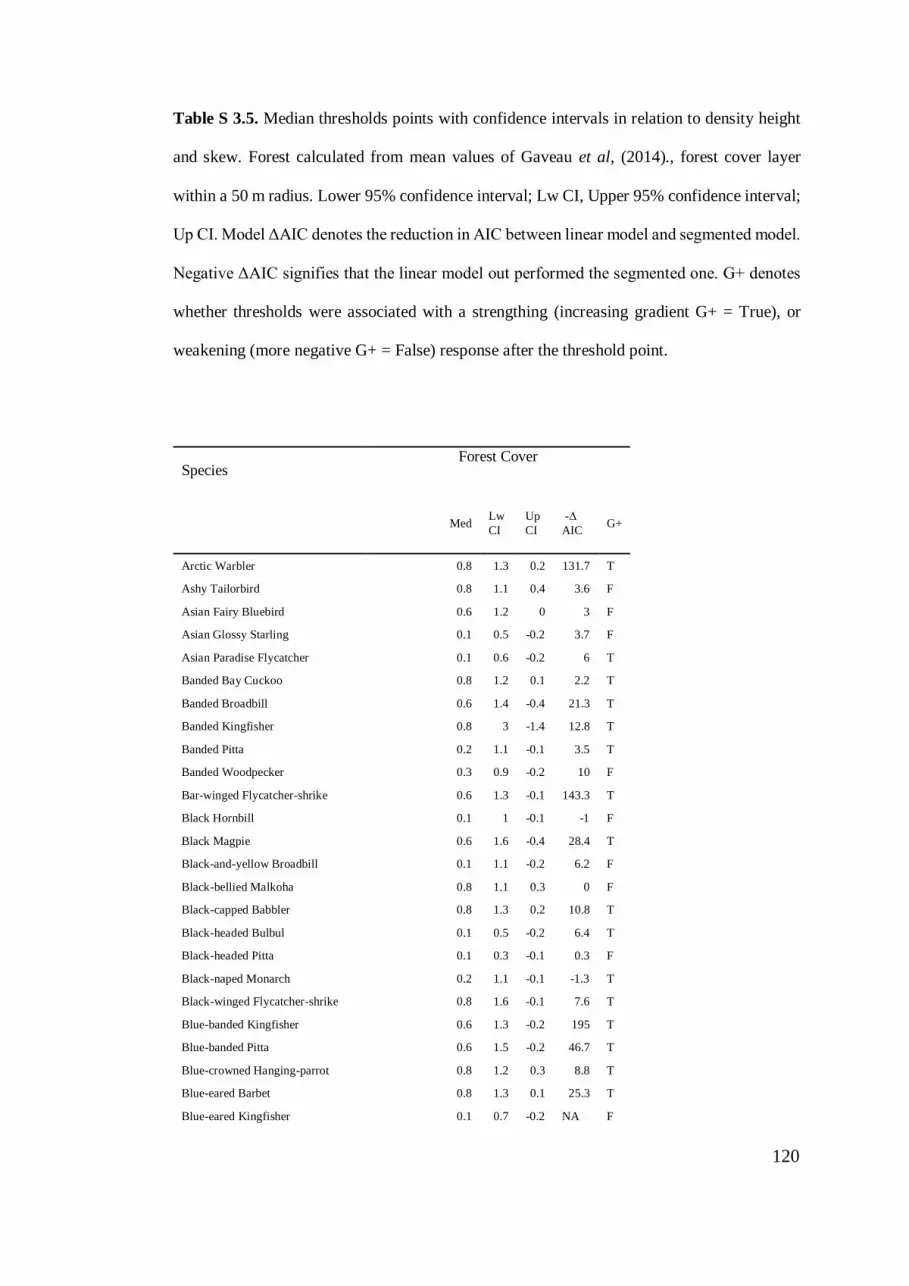
120
Table S 3.5. Median thresholds points with confidence intervals in relation to density height
and skew. Forest calculated from mean values of Gaveau et al, (2014)., forest cover layer
within a 50 m radius. Lower 95% confidence interval; Lw CI, Upper 95% confidence interval;
Up CI. Model ΔAIC denotes the reduction in AIC between linear model and segmented model.
Negative ΔAIC signifies that the linear model out performed the segmented one. G+ denotes
whether thresholds were associated with a strengthing (increasing gradient G+ = True), or
weakening (more negative G+ = False) response after the threshold point.
Species Forest Cover
Med Lw
CI
Up
CI
-Δ
AIC G+
Arctic Warbler 0.8 1.3 0.2 131.7 T
Ashy Tailorbird 0.8 1.1 0.4 3.6 F
Asian Fairy Bluebird 0.6 1.2 0 3 F
Asian Glossy Starling 0.1 0.5 -0.2 3.7 F
Asian Paradise Flycatcher 0.1 0.6 -0.2 6 T
Banded Bay Cuckoo 0.8 1.2 0.1 2.2 T
Banded Broadbill 0.6 1.4 -0.4 21.3 T
Banded Kingfisher 0.8 3 -1.4 12.8 T
Banded Pitta 0.2 1.1 -0.1 3.5 T
Banded Woodpecker 0.3 0.9 -0.2 10 F
Bar-winged Flycatcher-shrike 0.6 1.3 -0.1 143.3 T
Black Hornbill 0.1 1 -0.1 -1 F
Black Magpie 0.6 1.6 -0.4 28.4 T
Black-and-yellow Broadbill 0.1 1.1 -0.2 6.2 F
Black-bellied Malkoha 0.8 1.1 0.3 0 F
Black-capped Babbler 0.8 1.3 0.2 10.8 T
Black-headed Bulbul 0.1 0.5 -0.2 6.4 T
Black-headed Pitta 0.1 0.3 -0.1 0.3 F
Black-naped Monarch 0.2 1.1 -0.1 -1.3 T
Black-winged Flycatcher-shrike 0.8 1.6 -0.1 7.6 T
Blue-banded Kingfisher 0.6 1.3 -0.2 195 T
Blue-banded Pitta 0.6 1.5 -0.2 46.7 T
Blue-crowned Hanging-parrot 0.8 1.2 0.3 8.8 T
Blue-eared Barbet 0.8 1.3 0.1 25.3 T
Blue-eared Kingfisher 0.1 0.7 -0.2 NA F

121
Blue-headed Pitta 0.5 1.2 -0.2 -0.9 F
Blue-throated Bee-eater 0.8 1.2 0.2 -1 T
Bold-striped Tit-babbler 0.8 1.2 0.4 5.9 T
Bornean Blue Flycatcher 0.6 1.2 -0.1 8.7 F
Bornean Bristlehead 0.5 1.1 -0.1 11.7 T
Bornean Ground-cuckoo 0.1 0.7 -0.3 12.2 T
Bornean Wren-babbler 0.1 0.4 -0.2 472.4 T
Bronzed Drongo 0.1 0.4 -0.2 138.9 F
Brown Barbet 0.4 1 -0.1 11.2 F
Brown Flycatcher 0.8 1.6 0 23.4 T
Brown Fulvetta 0.1 0.2 -0.1 103.7 F
Brown-throated Sunbird 0.6 1.2 -0.1 5.8 T
Buff-rumped Woodpecker 0.8 1.4 0.2 29.3 T
Buff-vented Bulbul 0.1 0.4 -0.2 175.8 F
Bushy-crested Hornbill 0.6 1.4 -0.2 12.9 F
Checker-throated Woodpecker 0.1 1 -0.2 18.5 F
Chestnut Munia 0.6 1.2 -0.2 10.6 F
Chestnut-backed Scimitar-babbler 0.8 1.3 0.4 3.5 F
Chestnut-breasted Malkoha 0.1 1 -0.2 106 F
Chestnut-naped Forktail 0.6 1.4 -0.5 8.7 F
Chestnut-necklaced Partridge 0.1 0.7 -0.3 7.1 F
Chestnut-rumped Babbler 0.2 1.1 -0.1 6.6 F
Chestnut-winged Babbler 0.8 1.4 0.2 11 T
Collared Kingfisher 0.8 1.3 0 18.8 T
Cream-vented Bulbul 0.1 0.5 -0.4 543.5 T
Crested Fireback 0.1 0.7 -0.3 398.5 T
Crested Goshawk 0.1 0.7 -0.3 24 T
Crested Jay 0.8 1.2 0.3 15.8 T
Crested Serpent-eagle 0.1 0.3 -0.1 373.2 F
Crimson Sunbird 0.8 1.2 0.2 51.3 T
Crimson-winged Woodpecker 0.7 1.4 -0.1 33 T
Dark-necked Tailorbird 0.5 1.2 -0.3 4.2 T
Dark-sided Flycatcher 0.1 0.8 -0.1 12.8 F
Dark-throated Oriole 0.7 1.5 -0.2 41 T
Diards Trogon 0.8 1.3 -0.1 11.9 T
Drongo Cuckoo 0.6 1.3 -0.2 -1.7 F
Dusky Broadbill 0.1 0.2 -0.1 362.4 F
Dusky Munia 0.8 1.2 0.4 24.4 T
Emerald Dove 0.5 1.1 -0.1 17.8 F
Ferruginous Babbler 0.1 1 -0.1 8.3 F
Fiery Minivet 0.1 0.4 -0.3 22.8 F
Finschs Bulbul 0.8 1.2 0.4 18 F
Fluffy-backed Tit-babbler 0.8 1.2 0.4 23.4 T
Golden-bellied Gerygone 0.8 1.3 0 28.8 T
Gold-whiskered Barbet 0.1 1 -0.1 1.5 F

122
Great Argus 0.8 1.1 0.3 0.3 T
Great Slaty Woodpecker 0.1 0.6 -0.3 209.2 F
Greater Coucal 0.8 1.3 0.3 17.5 T
Greater Green Leafbird 0.5 1.2 -0.2 6.7 F
Greater Racket-tailed Drongo 0.5 1.3 -0.2 24.3 F
Green Broadbill 0.8 1.4 0.2 16.1 T
Green Imperial Pigeon 0.8 1.3 0.1 20.9 T
Green Iora 0.1 1.2 -0.3 101.2 F
Grey Wagtail 0.8 1.4 0.2 58.2 T
Grey-and-buff Woodpecker 0.1 0.3 -0.1 310 F
Grey-bellied Bulbul 0.6 1.2 -0.2 78 T
Grey-cheeked Bulbul 0.6 1.1 -0.1 2.5 F
Grey-chested Jungle-flycatcher 0.8 1.4 0.2 39.6 T
Grey-headed Babbler 0.6 1.6 -0.5 11.1 T
Grey-headed Canary-flycatcher 0.1 1.1 -0.2 22.9 T
Grey-rumped Treeswift 0.1 0.4 -0.1 -0.7 T
Hairy-backed Bulbul 0.1 0.5 -0.1 9.1 T
Helmeted Hornbill 0.1 0.3 -0.1 17.3 T
Hill Myna 0.3 1.2 -0.2 0.9 T
Hooded Pitta 0.8 1.1 0.4 4.9 T
Horsfields Babbler 0.8 1.2 0.4 10.9 F
Large Green Pigeon 0.1 0.6 -0.3 528.9 T
Large Woodshrike 0.8 1.3 0.2 8.4 T
Lesser Coucal 0.1 0.6 -0.2 161.3 F
Lesser Green Leafbird 0.1 0.3 -0.1 36 F
Little Egret 0.6 1.3 -0.1 20.8 T
Little Green Pigeon 0.8 1.3 0.2 9.1 T
Little Spiderhunter 0.5 1.1 -0.1 2.8 T
Long-billed Spiderhunter 0.6 1.3 -0.2 12.2 T
Long-tailed Parakeet 0.8 1.3 0.1 31.3 T
Malaysian Blue Flycatcher 0.6 1.3 0 29.5 T
Maroon Woodpecker 0 0.2 -0.1 175.8 F
Maroon-breasted Philentoma 0 0.2 -0.1 13.1 F
Moustached Babbler 0.8 1.2 0.2 20.4 T
Olive-backed Woodpecker 0.1 0.3 -0.2 606.6 T
Olive-winged Bulbul 0.1 0.6 -0.1 23.5 F
Orange-backed Woodpecker 0.1 1.3 -0.4 102.1 T
Orange-bellied Flowerpecker 0.8 1.4 -0.1 29.5 T
Oriental Dwarf Kingfisher 0.6 1.3 -0.1 20.9 T
Oriental Honey Buzzard 0.6 1.3 -0.3 1.5 F
Oriental Magpie Robin 0.7 1.2 -0.1 22 T
Pied Fantail 0.2 0.9 0 -0.3 F
Plain Sunbird 0.8 1.2 0.4 28.5 T
Plaintive Cuckoo 0.8 1.3 0.2 30 T
Puff-backed Bulbul 0.3 1.2 -0.2 2.7 T

123
Purple-naped Sunbird 0.8 1.2 0.4 2.7 F
Pygmy White-eye 0.1 1.8 -0.8 -0.1 T
Raffless Malkoha 0.8 1.2 0.4 5.1 T
Red-bearded Bee-eater 0.1 1.8 -0.9 6.5 T
Red-billed Malkoha 0.3 1.3 -0.4 -0.6 F
Red-eyed Bulbul 0.6 1.2 -0.3 153.5 T
Red-naped Trogon 0.8 1.3 0.2 42.7 T
Red-throated Barbet 0.8 1.2 0.3 19.6 T
Red-throated Sunbird 0.1 1.1 -0.1 9.5 F
Rhinoceros Hornbill 0.6 1.3 0.1 44.6 T
Ruby-cheeked Sunbird 0.8 1.3 0.1 19.4 T
Rufous Piculet 0.1 0.5 -0.3 1.1 F
Rufous Woodpecker 0.6 1.1 0.1 8 F
Rufous-chested Flycatcher 0.1 0.6 -0.1 9 F
Rufous-crowned Babbler 0.8 1.3 0.1 27.7 T
Rufous-fronted Babbler 0.1 1.1 -0.3 -2.6 F
Rufous-tailed Shama 0.6 1.1 0 4.3 T
Rufous-tailed Tailorbird 0.1 0.3 -0.1 -2.3 F
Rufous-winged Philentoma 0.1 1.1 -0.1 220.9 F
Scaly-crowned Babbler 0.3 1.2 -0.3 5.4 F
Scarlet Minivet 0 0.2 -0.1 18.2 F
Scarlet-rumped Trogon 0.1 0.6 0 NA F
Short-tailed Babbler 0.8 1.3 0 34.7 T
Short-toed Coucal 0.6 1.1 0.1 4.9 F
Slender-billed Crow 0.1 1.4 -0.5 67.4 T
Sooty-capped Babbler 0.8 1.2 0.4 16.3 T
Spectacled Bulbul 0.1 0.4 -0.2 373.5 F
Spectacled Spiderhunter 0.8 1.5 0 40.5 F
Spotted Dove 0 0.2 -0.1 25.2 T
Spotted Fantail 0.6 1.2 -0.1 19.5 T
Stork-billed Kingfisher 0.8 1.2 0.5 16.8 F
Streaked Bulbul 0.7 1.3 0 18.1 T
Streaky-breasted Spiderhunter 0.1 0.3 -0.1 112.2 F
Striped Wren-babbler 0.8 1.4 0.3 27 T
Thick-billed Green-pigeon 0.1 0.5 0 5 T
Tree Sparrow 0.1 1.1 -0.2 NA F
Van Hassalts Sunbird 0.5 1.4 -0.3 47.1 T
Velvet fronted Nuthatch 0.8 1.2 0.3 5.2 T
Verditer Flycatcher 0.6 1.4 -0.1 93.6 T
Violet Cuckoo 0.1 1.2 -0.4 -2.6 F
Wallacess Hawk-Eagle 0.6 1.6 -0.5 73.3 T
Whiskered Treeswift 0.1 0.5 -0.3 5 F
White-bellied Erpornis 0.8 1.2 0 10.2 T
White-bellied Woodpecker 0.4 1.3 -0.3 7.1 T
White-chested Babbler 0.8 1.4 0.2 41.3 T

124
White-crowned Forktail 0.5 1.3 -0.3 24 T
White-crowned Shama 0.1 0.5 -0.3 11.4 F
Wreathed Hornbill 0.8 1.1 0.4 5.5 T
Yellow-bellied Bulbul 0.8 2.3 -1.2 102.7 T
Yellow-bellied Prinia 0.1 0.7 0 -1 T
Yellow-breasted Flowerpecker 0.6 1.3 -0.1 13.4 T
Yellow-crowned Barbet 0.1 0.6 -0.1 47.7 F
Yellow-eared Spiderhunter 0.1 0.5 -0.1 327.7 F
Yellow-rumped Flowerpecker 0.1 1 -0.6 3.9 T
Yellow-vented Bulbul 0.6 1.2 -0.1 58.3 T
Yellow-vented Flowerpecker 0.8 1.2 0.4 11.7 T
Zebra Dove 0.8 1.3 0.3 26.9 T
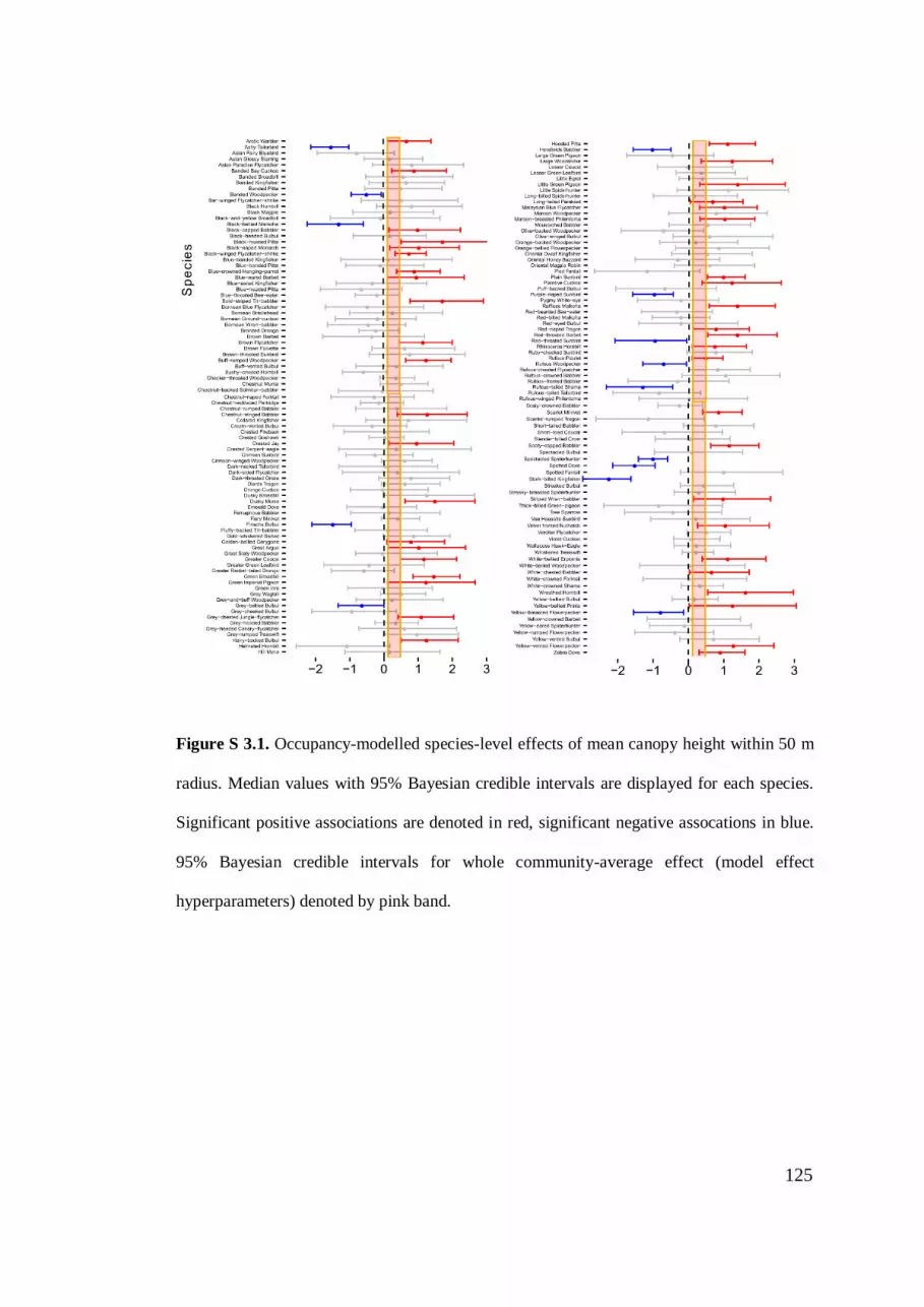
125
Figure S 3.1. Occupancy-modelled species-level effects of mean canopy height within 50 m
radius. Median values with 95% Bayesian credible intervals are displayed for each species.
Significant positive associations are denoted in red, significant negative assocations in blue.
95% Bayesian credible intervals for whole community-average effect (model effect
hyperparameters) denoted by pink band.

126
Figure S 3.2. Occupancy-modelled species-level effects of canopy heterogeneity with 50 m
radius. Median values with 95% Bayesian credible intervals are displayed for each species.
Significant positive associations are denoted in red. 95% Bayesian credible intervals for whole
community average effect (model effect hyperparameters) denoted by pink band.

127
Figure S 3.3. Occupancy-modelled species-level effects of mean vegetation density within 50
m radius. Median values with 95% Bayesian credible intervals are displayed for each species.
Significantly positive associations are denoted in red, significant negative assocations in blue.
95% Bayesian credible intervals for whole community average effect (model effect
hyperparameters) denoted by pink band.
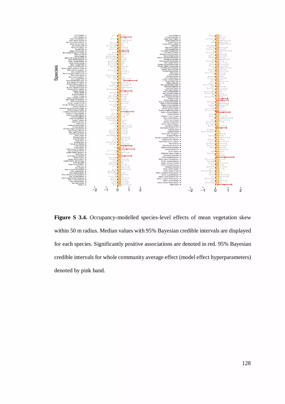
128
Figure S 3.4. Occupancy-modelled species-level effects of mean vegetation skew
within 50 m radius. Median values with 95% Bayesian credible intervals are displayed
for each species. Significantly positive associations are denoted in red. 95% Bayesian
credible intervals for whole community average effect (model effect hyperparameters)
denoted by pink band.
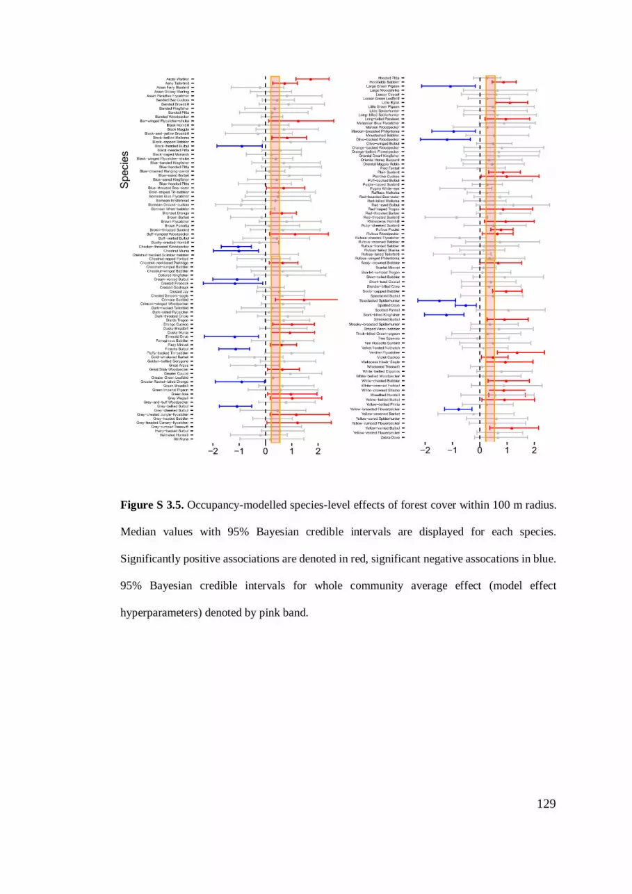
129
Figure S 3.5. Occupancy-modelled species-level effects of forest cover within 100 m radius.
Median values with 95% Bayesian credible intervals are displayed for each species.
Significantly positive associations are denoted in red, significant negative assocations in blue.
95% Bayesian credible intervals for whole community average effect (model effect
hyperparameters) denoted by pink band.

130
Figure S 3.6. Boxplots showing the distribution of threshold levels for different strata
associatons, feeding guilds and habitat assocations (pale blue, pale green and dark blue
respectively) listed for each environmental metric: a) mean canopy height in 50 m radius; b)

131
canopy heterogeneity in 50 m radius; c) mean vegetation density in 50 m radius; d) mean skew
in 50 m radius; e) mean forest cover in 50 m radius. Red dots indicate species with significant
positive effects. Blue dots are species with significant negative effects. Grey dots indicate no
significant effect. The size of dots correspond to the abundance of each species across the
global dataset. Larger sub-panels for each metric (left side) denote all species for which
segmented models had reduction in ΔAIC >4. Upper right panels denote the subset of species
where thresholds were associated with decreasing gradient of reponse. Lower right panels
denote the subset of species where thresholds were associated with increasing gradient of
reponse.

132
Table S 3.6. Results of Kruskal Wallis tests for differences in group average effects and
threshold levels between trait groups (Fig. S6). Results are given for each environmental
metric included in the overall occupancy model.
Environmental metric / group statistic parameter p value
Canopy height effects strata 1.5 2 0.472
Canopy height effects guilds 1.47 5 0.916
Canopy height effects habitat groups 9.54 4 0.049
Canopy height +g thresholds strata groups 0.49 2 0.784
Canopy height +g thresholds guilds 4.84 5 0.435
Canopy height +g thresholds habitat groups 6.66 4 0.155
Canopy height -g thresholds strata groups 1.84 2 0.399
Canopy height -g thresholds guilds 3.52 5 0.62
Canopy height -g thresholds habitat groups 5.93 4 0.205
Canopy heterogen. effects strata 2.39 3 0.495
Canopy heterogen. effects guilds 1.54 4 0.819
Canopy heterogen. effects habitat groups 2.56 4 0.634
Canopy heterogen. +g thresholds strata groups 5.45 3 0.142
Canopy heterogen. +g thresholds guilds 2.33 4 0.675
Canopy heterogen. +g thresholds habitat groups 0.96 4 0.916
Canopy heterogen. -g thresholds strata groups 2.02 3 0.568
Canopy heterogen. -g thresholds guilds 1.62 4 0.805
Canopy heterogen. -g thresholds habitat groups 3.24 4 0.518
Vegetation density effects strata 2.04 2 0.36
Vegetation density effects guilds 3.85 5 0.571
Vegetation density effects habitat groups 2.88 4 0.578
Vegetation density +g thresholds strata groups 1.45 2 0.485
Vegetation density +g thresholds guilds 3.43 5 0.634
Vegetation density +g thresholds habitat groups 2.11 4 0.716
Vegetation density -g thresholds strata groups 3.97 2 0.138
Vegetation density -g thresholds guilds 4.26 5 0.513
Vegetation density -g thresholds habitat groups 6.37 4 0.173
Vegetation skew effects strata 5.38 2 0.068
Vegetation skew effects guilds 8.53 6 0.202
Vegetation skew effects habitat groups 5.53 4 0.237
Vegetation skew +g thresholds strata groups 2.87 2 0.238
Vegetation skew +g thresholds guilds 3.45 5 0.631
Vegetation skew +g thresholds habitat groups 1.11 4 0.893
Vegetation skew -g thresholds strata groups 2.21 2 0.331
Vegetation skew -g thresholds guilds 5.89 5 0.317
Vegetation skew -g thresholds habitat groups 5.2 4 0.268
Forest cover (100m r) effects strata 0.44 2 0.804
Forest cover (100m r) effects guilds 1.52 5 0.911

133
Forest cover (100m r) effects habitat groups 4.34 4 0.362
Forest cover (100m r) +g thresholds strata groups 0.81 2 0.669
Forest cover (100m r) +g thresholds guilds 4.73 5 0.45
Forest cover (100m r) +g thresholds habitat groups 2.95 4 0.567
Forest cover (100m r) -g thresholds strata groups 0.31 2 0.855
Forest cover (100m r) -g thresholds guilds 4.7 5 0.453
Forest cover (100m r) -g thresholds habitat groups 3.63 4 0.458

134
Ackowledgements
This study was funded by the UK Natural Environment Research Council (NERC)
(NE/K016407/1; http://lombok.hmtf.info/ and http://bali.hmtf.info; NE/K016377/1),
and a Newton-Ungku Omar Fund grant from the British Council and Malaysia
Industry-Group for High Technology (MIGHT) (216433953). SLM was supported by
a PhD scholarship jointly funded by University of Kent and NERC. We thank the
Sabah Biodiversity Council, Sabah Forest Department, Yayasan Sabah, Sime Darby,
Benta Wawasan, Sabah Softwoods and Innoprise Foundation for permitting site
access. We are grateful to Unding Jami and the LOMBOK research assistant team for
their field assistance, and Suzan Benedic and Ryan Gray for facilitating fieldwork.
References
Andersen, T., Carstensen, J., Hernández-García, E. & Duarte, C.M. (2009) Ecological
thresholds and regime shifts: approaches to identification. Trends in Ecology and
Evolution, 24, 49–57.
Baker, M.E. & King, R.S. (2010) A new method for detecting and interpreting
biodiversity and ecological community thresholds. Methods in Ecology and
Evolution, 1, 25–37.
Baker, M.E. & King, R.S. (2013) Of TITAN and straw men: an appeal for greater
understanding of community data. Freshwater Science, 32, 489–506.
Banks-Leite, C., Renata, P., Tambosi, L.R., Pearse, W.D., Bueno, A.A., Bruscagin,
R.T., Condez, T.H., Dixo, M., Igari, A.T., Martensen, A.C. & P, M.J. (2014)

135
Using ecological thresholds to evaluate the costs and benefits of set-asides in a
biodiversity hotspot. , 345, 1041–1045.
Barragán, F., Moreno, C.E., Escobar, F., Halffter, G. & Navarrete, D. (2011) Negative
impacts of human land use on dung beetle functional diversity. PLoS ONE, 6.
Bergman, K.O., Askling, J., Ekberg, O., Ignell, H., Wahlman, H. & Milberg, P. (2004)
Landscape effects on butterfly assemblages in an agricultural region. Ecography,
27, 619–628.
Betts, M.G., Forbes, G.J. & Diamond, A.W. (2007) Thresholds in songbird occurrence
in relation to landscape structure. Conservation Biology, 21, 1046–1058.
Betts, A.M.G., Hagar, J.C., Rivers, J.W., Alexander, J.D., Mcgarigal, K. &
Applications, E. (2010) Thresholds in forest bird occurrence as a function of the
amount of early-seral broadleaf forest at landscape scales. Ecological
Applications, 20, 2116–2130.
Cardinale, B.J., Duffy, J.E., Gonzalez, A., Hooper, D.U., Perrings, C., Venail, P.,
Narwani, A., MacE, G.M., Tilman, D., Wardle, D.A., Kinzig, A.P., Daily, G.C.,
Loreau, M., Grace, J.B., Larigauderie, A., Srivastava, D.S. & Naeem, S. (2012)
Biodiversity loss and its impact on humanity. Nature, 486, 59–67.
Carigan, V. & Villard, M.-A. (2002) Selecting indicator species to monitor ecological
integrity: a review. Environmental Monitoring and Assessment, 78, 45–61.
Carpenter, S.R., Ludwig, D. & Brock, W.A. (1999) Management of eutrophication for
lakes subject to potentially irreversible change. Ecological Applications, 9, 751–
771.

136
Carginan, V., & Villard, M. A. (2002). Selecting indicator species to monitor
ecological integrity: a review. Environmental Monitoring and Assessment, 78(1),
45-61.
Ceballos, G., García, A., Pringle, R.M., Ceballos, G., Ehrlich, P.R., Barnosky, A.D.,
García, A., Pringle, R.M. & Palmer, T.M. (2015) Accelerated modern human –
induced species losses : Entering the sixth mass extinction. Science Advances, 1,
1–6.
Chapman, P. M., Tobias, J. A., Edwards, D. P., & Davies, R. G. (2018). Contrasting
impacts of land‐use change on phylogenetic and functional diversity of tropical
forest birds. Journal of Applied Ecology, 55(4), 1604-1614.
Cleary, D.F.R., Boyle, T.J.B., Setyawati, T., Anggraeni, C.D., Loon, E. Van &
Menken, S.B.J. (2012) Bird species and traits assocaited with logged and
unlogged forest in Borneo. Ecological Applications, 17, 1184–1197.
Cleary, D.F.R., Genner, M.J., Boyle, T.J.B., Setyawati, T., Angraeti, C.D. & Menken,
S.B.J. (2005) Associations of bird species richness and community composition
with local and landscape-scale environmental factors in Borneo. Landscape
Ecology, 20, 989–1001.
Davidson, A.D., Hamilton, M.J., Boyer, A.G., Brown, J.H. & Ceballos, G. (2009)
Multiple ecological pathways to extinction in mammals. Proceedings of the
National Academy of Sciences, 106, 10702–10705.
Davies, A.B. & Asner, G.P. (2014) Advances in animal ecology from 3D-LiDAR
ecosystem mapping. Trends in Ecology and Evolution, 29, 681–691.

137
DeAngelis, D. L. (2018). Individual-based models and approaches in ecology:
populations, communities and ecosystems. CRC Press.
Deere, N.J., Guillera-Arroita, G., Baking, E.L., Bernard, H., Pfeifer, M., Reynolds, G.,
Wearn, O.R., Davies, Z.G. & Struebig, M.J. (2018) High Carbon Stock forests
provide co-benefits for tropical biodiversity. Journal of Applied Ecology, 55,
997–1008.
del Hoyo, J., Elliott, A., Sargatal, J., Christie, D.A. & de Juana, E. (eds.). Handbook
of the Birds of the World Alive. Lynx Edicions, Barcelona. (retrieved from
https://www.hbw.com/node/467146 on 30 January 2019).
Devictor, V., Julliard, R. & Jiguet, F. (2008) Distribution of specialist and generalist
species along spatial gradients of habitat disturbance and fragmentation. Oikos,
117, 507–514.
Dieleman, C.M., Branfireun, B.A., Mclaughlin, J.W. & Lindo, Z. (2015) Climate
change drives a shift in peatland ecosystem plant community: Implications for
ecosystem function and stability. Global Change Biology, 21, 388–395.
Dorazio, R.M. & Royle, J.A. (2005) Estimating size and composition of biological
communities by modeling the occurrence of species. Journal of the American
Statistical Association, 100, 389–398.
Edwards, D.P., Ansell, F.A., Ahmad, A.H., Nilus, R. & Hamer, K.C. (2009) The value
of rehabilitating logged rainforest for birds. Conservation Biology, 23, 1628–
1633.
Ellis, E.C. (2011) Anthropogenic transformation of the terrestrial biosphere.
Philosophical Transactions of the Royal Society A: Mathematical, Physical and

138
Engineering Sciences, 369, 1010–1035.
Evans-White, M.A., Dodds, W.K., Huggins, D.G. & Baker, D.S. (2009) Thresholds
in macroinvertebrate biodiversity and stoichiometry across water-quality
gradients in Central Plains (USA) streams. Journal of the North American
Benthological Society, 28, 855–868.
Folke, C., Carpenter, S., Walker, B., Scheffer, M., Elmqvist, T., Gunderson, L., &
Holling, C. S. (2004). Regime shifts, resilience, and biodiversity in ecosystem
management. Annual Review Ecology Evolution and Systematics, 35, 557-581.
França, F.M., Frazão, F.S., Korasaki, V., Louzada, J. & Barlow, J. (2017) Identifying
thresholds of logging intensity on dung beetle communities to improve the
sustainable management of Amazonian tropical forests. Biological Conservation,
216, 115–122.
Gardner, T.A., Barlow, J., Araujo, I.S., Ávila-Pires, T.C., Bonaldo, A.B., Costa, J.E.,
Esposito, M.C., Ferreira, L. V., Hawes, J., Hernandez, M.I.M., Hoogmoed, M.S.,
Leite, R.N., Lo-Man-Hung, N.F., Malcolm, J.R., Martins, M.B., Mestre, L.A.M.,
Miranda-Santos, R., Overal, W.L., Parry, L., Peters, S.L., Ribeiro, M.A., Da
Silva, M.N.F., Da Silva Motta, C. & Peres, C.A. (2008) The cost-effectiveness
of biodiversity surveys in tropical forests. Ecology Letters, 11, 139–150.
Gerstner, K., Dormann, C.F., Stein, A., Manceur, A.M. & Seppelt, R. (2014) Effects
of land use on plant diversity - A global meta-analysis. Journal of Applied
Ecology, 51, 1690–1700.
Gibson, L., Ming Lee, T., Koh, L.P., Brook, B.W., Gardner, T.A., Barlow, J., Peres,
C.A., Bradshaw, C.J.A., Laurance, W.F., Lovejoy, T.E. & Sodhi, N.S. (2011)

139
Primary forests are irreplaceable for sustaining tropical biodiversity. Nature, 478,
378–381.
Groffman, P.M., Baron, J.S., Blett, T., Gold, A.J., Goodman, I., Gunderson, L.H.,
Levinson, B.M., Palmer, M.A., Paerl, H.W., Peterson, G.D., Poff, N.L.R.,
Rejeski, D.W., Reynolds, J.F., Turner, M.G., Weathers, K.C. & Wiens, J. (2006)
Ecological thresholds: The key to successful environmental management or an
important concept with no practical application? Ecosystems, 9, 1–13.
Haddad, N.M., Brudvig, L.A., Clobert, J., Davies, K.F., Gonzalez, A., Holt, R.D.,
Lovejoy, T.E., Sexton, J.O., Austin, M.P., Collins, C.D., Cook, W.M.,
Damschen, E.I., Ewers, R.M., Foster, B.L., Jenkins, C.N., King, A.J., Laurance,
W.F., Levey, D.J., Margules, C.R., Melbourne, B.A., Nicholls, A.O., Orrock,
J.L., Song, D. & Townshend, J.R. (2015) Applied Ecology: Habitat
fragmentation and its lasting impact on Earth ’ s ecosystems. Science Advances,
1, 1–9.
Hevia, V., Martín‐López, B., Palomo, S., García‐Llorente, M., de Bello, F., &
González, J. A. (2017). Trait‐based approaches to analyze links between the
drivers of change and ecosystem services: Synthesizing existing evidence and
future challenges. Ecology and Evolution, 7, 831-844.
Hirota, M., Homgren, M., Van Nes, E.H. & Scheffer, M. (2011) Global resilience of
tropical forest and savanna to critical transitions. Science, 334, 232–234.
Hutter, M. (2005) Bayesian regression of piecewise constant functions. , 635–664.
Jones, K.E., Purvis, A. & Gittleman, J.L. (2003) Biological correlates of extinction
Risk in Bats. The American Naturalist, 161, 601–614.
140
Kays, R. & Allison, A. 2001. Arboreal tropical forest vertebrates: current knowledge
and research trends. Plant Ecology, 153, 109-120.
Kellner, K. (2016). jagsUI: A Wrapper Around ‘rjags’ to Streamline ‘JAGS’Analyses.
Version 1.4. 2.
Lambert, F. R. (1992). The consequences of selective logging for Bornean lowland
forest birds. Phil. Trans. R. Soc. Lond. B, 335(1275), 443-457.
Laurance, S.G. (2004) Responses of understory rainforest birds to road edges in
Central Amazonia. Ecological Applications, 14, 1344–1357.
Laurance, W. F., Useche, D. C., Rendeiro, J., Kalka, M., Bradshaw, C. J., Sloan, S. P.,
& Arroyo-Rodriguez, V. (2012). Averting biodiversity collapse in tropical forest
protected areas. Nature, 489, 290.
Lavorel, S., & Garnier, É. (2002). Predicting changes in community composition and
ecosystem functioning from plant traits: revisiting the Holy Grail. Functional
Ecology, 16(5), 545-556.
Lindenmayer, D.B., Fischer, J. & Cunningham, R.B. (2005) Native vegetation cover
thresholds associated with species responses. Biological Conservation, 124, 311–
316.
Lu, N., Jia, C.X., Lloyd, H. & Sun, Y.H. (2012) Species-specific habitat fragmentation
assessment, considering the ecological niche requirements and dispersal
capability. Biological Conservation, 152, 102–109.
Maas, B., Tscharntke, T., Saleh, S., Dwi Putra, D., & Clough, Y. (2015). Avian species
identity drives predation success in tropical cacao agroforestry. Journal of
Applied Ecology, 52(3), 735-743.

141
Martensen, A.C., Ribeiro, M.C., Banks-Leite, C., Prado, P.I. & Metzger, J.P. (2012)
Associations of forest cover, fragment area, and connectivity with Neotropical
understory bird species richness and abundance. Conservation Biology, 26,
1100–1111.
Mattila, N., Kaitala, V., Komonen, A., Päivinen, J. & Kotiaho, J.S. (2011) Ecological
correlates of distribution change and range shift in butterflies. Insect
Conservation and Diversity, 4, 239–246.
May, 1977. (1977) Thresholds and breakpoints in ecosystems with a multiplicity of
stable states. Nature, 269, 471–477.
Melo, I., Ochoa-Quintero, J.M., de Oliveira Roque, F. & Dalsgaard, B. (2018) A
review of threshold responses of birds to landscape changes across the world.
Journal of Field Ornithology, 88.4, 303-314
Meron, E. (2015) Nonlinear Physics of Ecosystems. CRC Press; 2015.
Michael, D.R., Kay, G.M., Crane, M., Florance, D., Macgregor, C., Okada, S.,
Mcburney, L., Blair, D. & Lindenmayer, D.B. (2015) Ecological niche breadth
and microhabitat guild structure in temperate Australian reptiles: Implications for
natural resource management in endangered grassy woodland ecosystems.
Austral Ecology, 40, 651–660.
Muggeo, V.M.R. (2003) Estimating regression models with unknown break-points.
Statistics in Medicine, 22, 3055–3071.
Muggeo, V.M. (2008) segmented: An R package to fit regression models with broken-
line relationships. R news, 20–25, 1–73.

142
Murray, K.A., Rosauer, D., McCallum, H. & Skerratt, L.F. (2011) Integrating species
traits with extrinsic threats: Closing the gap between predicting and preventing
species declines. Proceedings of the Royal Society B: Biological Sciences, 278,
1515–1523.
Muylaert, R.L., Stevens, R.D. & Ribeiro, M.C. (2016) Bat richness decline along a
fragmentation threshold effect of habitat loss on bat richness in cerrado-forest
landscapes. Ecological Applications, 26, 1854–1867.
Newbold, T., Hudson, L.N., Hill, S.L.L., Contu, S., Lysenko, I., Senior, R.A., Börger,
L., Bennett, D.J., Choimes, A., Collen, B., Day, J., De Palma, A., Díaz, S.,
Echeverria-Londoño, S., Edgar, M.J., Feldman, A., Garon, M., Harrison, M.L.K.,
Alhusseini, T., Ingram, D.J., Itescu, Y., Kattge, J., Kemp, V., Kirkpatrick, L.,
Kleyer, M., Correia, D.L.P., Martin, C.D., Meiri, S., Novosolov, M., Pan, Y.,
Phillips, H.R.P., Purves, D.W., Robinson, A., Simpson, J., Tuck, S.L., Weiher,
E., White, H.J., Ewers, R.M., MacE, G.M., Scharlemann, J.P.W. & Purvis, A.
(2015) Global effects of land use on local terrestrial biodiversity. Nature, 520,
45–50.
Newbold, T., Scharlemann, J.P.W., Butchart, S.H.M., ¸ekerciog ˘lu, ˘an H S,
Alkemade, R., Booth, H. & Purves, D.W. (2013) Ecological Traits Affect the
Response of Tropical Forest Bird Species to Landuse Intensity. Proceedings of
The Royal Society B, 280, 20122131.
Nobre, C.A. & Borma, L.D.S. (2009) ‘Tipping points’ for the Amazon forest. Current
Opinion in Environmental Sustainability, 1, 28–36.
Oksanen, J. & Minchin, P. (2002) Continuum theory revisited: what shapes are species

143
reponses along ecological gradients. Ecological Modelling, 157, 119–129.
O'connell, T. J., Jackson, L. E., & Brooks, R. P. (1998). A bird community index of
biotic integrity for the mid-Atlantic highlands. Environmental Monitoring and
Assessment, 51, 145-156.
Pacifici, M., Visconti, P., Butchart, S.H.M., Watson, J.E.M., Cassola, F.M. &
Rondinini, C. (2017) Species’ traits influenced their response to recent climate
change. Nature Climate Change, 7, 205–208.
Pearson, R.G., Stanton, J.C., Shoemaker, K.T., Aiello-Lammens, M.E., Ersts, P.J.,
Horning, N., Fordham, D.A., Raxworthy, C.J., Ryu, H.Y., McNees, J. &
Akçakaya, H.R. (2014) Life history and spatial traits predict extinction risk due
to climate change. Nature Climate Change, 4, 217–221.
Peh, K.S.-H., Jong, J. De, Sodhi, N.S., Lim, S.L.-H. & Yap, C. a.-M. (2005) Lowland
rainforest avifauna and human disturbance: persistence of primary forest birds in
selectively logged forests and mixed-rural habitats of southern Peninsular
Malaysia. Biological Conservation, 123, 489–505.
Phalan, B. (2011) Reconciling food production and biodiversity conservation : Land
sharing and land sparing compared. Science, 333, 1289.
Plummer, M. (2003). JAGS: A program for analysis of Bayesian graphical models
using Gibbs sampling. In: Proceedings of the 3rd international workshop on
distributed statistical computing, 2003. Vienna, Austria.
Plummer, M. (2013). rjags: Bayesian graphical models using MCMC. R package
version, 3(10).
Piza-Roca, C., Zelfde, M. van ’t, Haye, M.J.J. La, Jongejans, E. & Raes, N. (2018)

144
European badger habitat requirements in the Netherlands – combining ecological
niche models with neighbourhood analysis. Wildlife Biology, 2018.
Radford, J.Q. & Bennett, A.F. (2004) Thresholds in landscape parameters: Occurrence
of the white-browed treecreeper Climacteris affinis in Victoria, Australia.
Biological Conservation, 117, 375–391.
Riddle, B.R. & Fafner, D.J. (1999) Species as units of analysis in ecology and
biogeography: time to take the blinders off. Global Ecology and Biogeography,
8, 433–441.
Riley, S.P.D., Busteed, G.T., Kats, L.B., Vandergon, T.L., Lee, L.F.S., Dagit, R.G.,
Kerby, J.L., Fisher, R.N. & Sauvajot, R.M. (2005) Effects of urbanization on the
distribution and abundance of amphibians and invasive species in southern
California streams. Conservation Biology, 19, 1894–1907.
Royle, J. A., & Dorazio, R. M. (2008). Hierarchical modelling and inference in
ecology: the analysis of data from populations, metapopulations and
communities. Elsevier.
Scheffer, M., Carpenter, S., & Foley, J. (2001). a, Folke C, Walker B. Catastrophic
shifts in ecosystems. Nature, 413, 591-6.Sekercioglu, C.H. (2007) Conservation
Ecology: Area trumps mobility in fragment bird extinctions. Current Biology, 17,
283–286.
Sheldon, F. H., Lim, H. C., Nais, J., Lakim, M., Tuuga, A., Malim, P., ... & Moyle, R.
G. (2009). Observations on the ecology, distribution, and biogeography of forest
birds in Sabah, Malaysia. Raffles Bulletin of Zoology, 57(2), 577-586.
Sheldon, F.H., Styring, A. & Hosner, P. a. (2010) Bird species richness in a Bornean

145
exotic tree plantation: A long-term perspective. Biological Conservation, 143,
399–407.
Siddig, A.A.H., Allison, A.M., Ochs, A., Villar-Leeman, C. & K, L.M. (2016) How
do ecologists select and use indicator species to monitor ecological change?
Insights from 14 years of publication in Ecological Indicators. Ecological
Indicators, 60, 223–239.
Silva, M., Hartling, L. & Opps, S.B. (2005) Small mammals in agricultural landscapes
of Prince Edward Island (Canada): Effects of habitat characteristics at three
different spatial scales. Biological Conservation, 126, 556–568.
Stratford, J.A. & Stouffer, P.C. (2013) Microhabitat associations of terrestrial
insectivorous birds in Amazonian rainforest and second-growth forests. Journal
of Field Ornithology, 84, 1–12.
Styring, A. R., Ragai, R., Unggang, J., Stuebing, R., Hosner, P. A., & Sheldon, F. H.
(2011). Bird community assembly in Bornean industrial tree plantations: effects
of forest age and structure. Forest Ecology and Management, 261(3), 531-
544.Suarez-Rubio, M. & Lookingbill, T.R. (2016) Forest birds respond to the
spatial pattern of exurban development in the Mid-Atlantic region, USA. PeerJ,
4, e2039.
Walker, B., Hansen, J., Corell, R.W., Fabry, V.J., Karlberg, L., Falkenmark, M.,
Svedin, U., Snyder, P.K., Costanza, R., Rodhe, H., Sörlin, S., Leeuw, S. van Der,
Hughes, T., Wit, C.A. de, Nykvist, B., Schellnhuber, H.J., Folke, C., Scheffer,
M., Lenton, T.M., Lambin, E., Chapin, F.S.I.I.I., Persson, Å., Noone, K., Steffen,
W., Rockström, J., Liverman, D., Richardson, K., Crutzen, P. & Foley, J. (2009)

146
Planetary Boundaries: Exploring the Safe Operating Space for Humanity.
Ecology and Society, 14, 32.
Williams, N.M., Crone, E.E., Roulston, T.H., Minckley, R.L., Packer, L. & Potts, S.G.
(2010) Ecological and life-history traits predict bee species responses to
environmental disturbances. Biological Conservation, 143, 2280–2291.
Wunderle, J.M., Henriques, L.M.P. & Willig, M.R. (2006) Short-term responses of
birds to forest gaps and understory: An assessment of reduced-impact logging in
a lowland Amazon forest. Biotropica, 38, 235–255.

147
Sound methods for monitoring tropical
biodiversity: Optimising acoustic indices to reflect
species richness in forest habitats
Simon L. Mitchell1, David P. Edwards2, Jake Bicknell1, Nicolas J. Deere1
David Coomes3, Henry Bernard4, Zoe G. Davies1, Matthew J Struebig1
1 Durrell Institute of Conservation and Ecology (DICE), School of Anthropology and
Conservation, University of Kent, Canterbury, CT2 7NR, UK
2 University of Sheffield, Western Bank, Sheffield, S10 2TN
3Forest Ecology and Conservation Group, Department of Plant Sciences, University
of Cambridge, Downing Street, Cambridge CB2 3EA, UK
4 Institute for Tropical Biology and Conservation, Universiti Malaysia Sabah, 88400
Kota Kinabalu, Sabah, Malaysia.

148
Abstract
Approaches to characterise and monitor biodiversity based on the sound
signals of ecosystems appear to offer great potential, with acoustic indices reflecting
avian species richness in a variety of environments. However, to date validation
studies of how well acoustic indices reflect observed patterns of biodiversity have
tended to use relatively low levels of spatial replication and have focussed on habitats
with similar underlying anthropological and geophysical sound characteristics. For
acoustic indices to be broadly applicable to biodiversity surveys and monitoring, their
capacity to measure the ecological facets of soundscapes must be robust to these
potential sources of bias. We examined the efficacy of five commonly used acoustic
indices to reflect patterns of observed and estimated avian species richness across a
land-cover gradient in Northeast Borneo. The gradient comprised intact forests to oil
palm plantations, thus providing a highly variable anthrophonic and geophonic
soundscape. We found that Acoustic Complexity had the strongest relationship with
observed bird richness in old growth forest and logged forest, but that Acoustic
Evenness had the strongest (negative) association with observed richness in riparian
areas. No acoustic indices were associated with observed richness in oil palm riparian
areas. We attempted to improve the associations between acoustic indices and species
richness by digitally reducing background noise outside of the vocal frequency range
for birds, controlling for time-of-day, and removing a habitat with high anthropogenic
influence. Our Adjusted Bioacoustic Index was better than unaggregated point counts
at capturing changes in species richness associated with changing canopy height, and
the association between the Adjusted Bioacoustic Index and canopy height was
comparable to that when species richness was estimated via occupancy-modelling.

149
Our findings underscore the potential utility of soundscape approaches to characterise
biodiversity patterns in human-modified tropical landscapes, but demonstrate that for
acoustic indices to be more effective the bias introduced by time-of-day, geophonic
noise, cicada choruses and human voices needs to be better accounted for.
Introduction
In the midst of the current environmental crisis (Rockstrom et al., 2009; Ripple
et al., 2017) conservation practitioners are seeking more efficient and cost-effective
ways of monitoring biodiversity (Bustamante et al., 2015). Recent advances have
included the application of new remote sensing technologies (Pettorelli et al., 2014),
such as the use of Light Detection And Ranging (LiDAR; Guo et al., 2017) and
Synthetic Aperture Radar (Villard et al., 2016) to identify species habitat associations
(Taft et al., 2003). Additional developments include, new statistical approaches to
derive robust estimates of species occupancy from sparse data for rare species (Royle
& Kery, 2007), novel methods environmental DNA procedure facilitating rapid impact
assessments (Valentini et al., 2006), and the use of autonomous wildlife surveillance
methods, such as camera traps and sound-recorders (Harrison et al., 2012).
The increased availability and reduced cost of sound-recorders has opened up
an entirely new field of conservation research and practice. Soundscape ecology is
concerned with the same basic principles and questions as landscape ecology,
including a focus on how acoustic signals in a particular location change with time,
habitat-disturbance, and patterns of biological and human activity (Gasc et al., 2016).
One of the main focuses of soundscape assessments is to discern patterns of

150
biodiversity (Pijanowski et al., 2006). This differs from the field of bioacoustics,
which tends to focus on the physics and variation of biological sound production
among organisms.
Birds are excellent surrogates for wider patterns of biodiversity (Lewandowski
et al., 2008; Gardner et al., 2008) and are also one of the most dominant terrestrial
taxonomic groups in terms of abundance, biomass and contribution to soundscapes
(Gasc et al., 2016). Due to these characteristics, they have been a focus of efforts to
characterise or estimate species richness and community structure from soundscape
recordings. A large number of indices have been developed to statistically describe
the distribution of acoustic information in a given recording. Some of these acoustic
indices seek to determine variation in anthropogenic disturbance (i.e. ‘anthrophony’;
Kasten et al., 2012), or acoustic dissimilarity between recordings (Sueur et al., 2008),
whilst the majority are designed to reflect the richness and complexity of ecological
communities, such as total acoustic complexity, entropy or bioacoustic activity (e.g
Pieretti et al., 2011; Sueur et al., 2008; Depraetere et al., 2012). Acoustic indices have
been applied across a wide variety of habitats and environmental contexts, including
investigating patterns of species richness in temperate reefs (Harris et al., 2016),
detecting the response of tropical wildlife to haze caused by forest fires (Lee et al,
2016), assessing avian richness in tropical open woodland savannah (Alequzar &
Machado 2015), monitoring freshwater lakes for invasive Tilapia (Kottege et al.,
2015), and quantifying patterns of species diversity in tropical forest (Mammides et
al., 2017).
A central assumption behind the application of acoustic indices is that greater
acoustic diversity reflects more vocal species in a given community (Gage et al.,

151
2001). It is also assumed that acoustic diversity is positively correlated with measures
of biodiversity and ecosystem functioning (Pijanowski et al 2011). For birds,
validation studies have compared acoustic indices directly with two established
methods for assessing species richness: point count data and expert identification of
birds from recordings (Darras et al., 2018). Acoustic indices correlate with avian
richness in temperate (Depraetere et al., 2012; Eldridge et al., 2018), sub-tropical
(Fuller et al., 2015) and tropical (Mammides et al., 2017) environments. Proponents
of soundscape ecology tend to advocate the use of sound-recorders as a more efficient
way of measuring bird diversity than expert ornithologists collecting survey data
(Eldrige et al., 2018). However, to date, acoustic validation attempts have used fairly
small datasets in terms of their spatial replication. For instance, Mammides et al.
(2017) used 97 sampling points for the deployment of autonomous recorders, across
seven landuse categories, Eldridge et al. (2018) used 90 sampling points, and Izaguirre
et al. (2018) used 60 sampling points. Other studies have concentrated on comparing
two different habitat types, which are often highly distinct from one another, such as
gallery forest compared to cerrado vegetation in Brazil (Machado et al., 2017). Thus,
while validations have provided useful insights into which metrics best correlate with
observed avian richness, it remains unclear whether such patterns remain consistent
over large spatial scales and complex environmental gradients. Similarly, the extent to
which such indices perform as reliable proxies for actual richness across habitats
containing varying levels of other acoustic signals, such as those from anthropogenic
and geo-physical sources, is uncertain. For example, recent work from urban areas in
the UK suggests that many acoustic indices do not perform well in landscapes with a
high contribution of anthrophonic signal (Fairbrass et al., 2017). Therefore,
determining which indices are consistently robust remains a research priority, as does

152
finding ways to optimise existing indices to avoid the biases introduced by potentially
confounding acoustic signals.
Here, we assess the performance of five commonly used acoustic indices in
reflecting variation in avian diversity across a land-cover gradient in Sabah, Malaysian
Borneo – a region characterised by exceptional levels of biodiversity, and intense
forest degradation and deforestation. Our species data were generated from point
counts conducted simultaneous with sound recordings, as well as highly precise
estimates of richness derived from a Bayesian occupancy model that accounts for
differences in species detection. Accounting for variation in detection probability is
currently another hurdle in improving the effectiveness of acoustic methods, since
detection probabilities vary between species and are not accounted for within indices.
We test a number of approaches to improve the potential association between acoustic
indices and diversity data, and compare the ability of each of these indices to capture
patterns of species richness across the landscape gradient. We also compare the
performance of acoustic indices in capturing changes in species richness associated
with canopy height across tropical forests, as derived from high-resolution LiDAR
data, to determine whether soundscape indices reflect habitat structure.
Methods
Bird sampling
Birds were sampled via 15-minute 50 m radius point counts at 373 localities
in five habitat types in Sabah, with three or four visits to each site between 2014 and
2017 (1,259 point counts in total; Chapter 3). These were carried out by a single

153
experienced observer (SLM) between 05:50am and 11:00am on days without rain.
Temporal independence between repeated point counts at a given site was ensured as
repeat counts at sites were always undertaken on different days. Spatial independence
was ensured by all sites being located at least 180 m from one another. Sound
recordings were taken simultaneously alongside each point count, using a single field
recorder (Olympus LS-11/LS-12) comprising dual cardioid microphones positioned
perpendicular to one another. In riparian areas, where background geophonic sound
from running water was sometimes significantly higher, the recorder was placed at
least 10 m from the fastest flowing sections of watercourses and oriented away from
areas producing the most noise.
Point count localities (total n=373) covered a gradient of habitat degradation
and increasing human presence, from unlogged old-growth dipterocarp forest to oil
palm plantations (Fig. 3.1, Chapter 3). Old-growth forests (n=50 point count locations)
were sampled at Danum Valley Conservation Area (n=20), Sepilok Forest Reserve
(n=20) and Maliau Basin Conservation Area (n=10). We surveyed riparian areas in
continuous logged forest (riparian forest; n=80), isolated riparian reserves within oil
palm plantations (riparian reserves, n=100), and riparian areas without natural
vegetation in oil palm estates (oil palm riparian; n=20) in and around the Stability of
Altered Forest Ecosystems (SAFE) landscape. Additionally, we sampled non-riparian
areas within the continuous logged forests within the SAFE area and the adjacent Ulu-
Segama Forest Reserve (logged forest; n=123).
Each habitat type supported not only a different ecological community
(Chapters 2 and 3), but also a different acoustic context. Anthropogenic noise levels
varied for each of these habitats, being associated with distant machinery from

154
adjacent logging, or agricultural operations and road and trail maintenance, the latter
being especially prominent within oil palm. Old-growth and selectively logged forests
comprised terra-firma lowland dipterocarps with low geophonic sound, while riparian
forests were situated on fast-flowing streams with variable levels of peak discharge
and high levels of background geophonic noise. Riparian reserves (i.e. those in the oil
palm estates) consisted of a few high-noise fast-flowing streams, but in general were
slower-flowing alluvial areas with few riffles or cascades resulting in lower levels of
geophonic noise than counterpart localities in the riparian forest. Although oil palm
riparian sites were located along water courses, these were all very small slow-flowing
streams with no significant sounds of running water (low geophonic influence).
Riparian forest and old-growth sites were located along streams or trails in transects
comprising 10 point counts, whilst point counts at logged forest sites followed the
SAFE fractal design (Ewers et al., 2015). This design uses constellations of points
spaced at least 180 m apart in groups of 16, which were undertaken as intersecting
transects of 8 points on separate days.
Acoustic Indices
The first minute of each sound recording included the observer stating the date,
time and location, and then moving away from the recorder. This sequence was
therefore cut from all recordings prior to analysis. We assessed five commonly used
acoustic indices over the remaining 14-minute portion of each recording: Acoustic
complexity (AC); Bioacoustic Index (BA); Acoustic Diversity (AD); Acoustic
Evenness (AE) and the Normalised Difference in Soundscape Index (NDSI). The

155
indices were quantified using the packages soundecology (Villanueva Rivera and
Pijanowski, 2013) and seewave-R (Sueur et al., 2008) in R (R Core Team, 2014).
Acoustic complexity is designed to capture the intricacy of biophonic signals,
while ignoring the influence of many anthrophonic and geophonic noises. It is based
on the premise that biotic sounds intrinsically encompass a large variety of intensities,
whereas sounds such as overflying airplanes or running water are associated with
constant intensity values (Pieretti & Morri, 2011). The Bioacoustic Index (BA)
describes mean spectral power between 2,000 kHz and 8,000 kHz, as this frequency
range covers most infrasonic ecological sound, but excludes many anthropogenic
noises which, in general, register below 2,000 kHz (Boelman et al., 2007). Acoustic
Diversity calculates Shannon’s diversity index for each recording based on the power
of each 1 kHz frequency band. Acoustic Evenness measures evenness between ten
equal frequency bands 0 – 22,050 kHz as the proportion of the signals in each band
above a -50 dBFS threshold, where dBFS is decibels relative to the ‘full scale’
maximum amplitude within a given file (Villanueva-Rivera et al. 2011). We also
computed the Normalised Difference in Soundscape Index (NDSI), which is simply
the ratio of biotic to anthropogenic signal (Kasten et al., 2012).
Acoustic Diversity is based on the Shannon-Wiener index (Jost, 2006) whereas
Acoustic Evenness, which is based on the Gini-Simpson index (Gini, 1997). These two
indices therefore characterise inverse soundscape properties to one another (Eldridge
2018). Therefore, after confirming this was also the case in our results (Table 4.1),
we opted to use only Acoustic Evenness since it showed stronger associations with
point count richness than Acoustic Diversity.

156
A pre-processing procedure was run on each of 1,299 recordings, following
the protocol used by Arnold (2013) to maximise the clarity of recordings for human
hearing. Using the free audio editing software Audacity (1999-2013 Audacity Team;
SourceForge.net), we first removed frequencies of >10,000kHz and <800kHz, using
high- and low-pass filters to remove extreme unwanted anthrophonic sounds, such as
traffic noise (e.g. Eldridge et al. 2018). We also added a small notch filter to remove
a narrow range of frequencies that included the commonest cicada chorus (7,950 -
8,050 kHz). In order to remove background noise we selected a two-minute section of
one of our riparian recordings in which only river sounds (and no biological signals)
could be detected by human examination. Using Audacity’s proprietary noise removal
process, we set this as a background ‘noise profile’ and used the specific profile to
determine where spectral power exceeded those of the background noise profile for
each 100 kHz frequency band in a recording (i.e not background signals that were
assumed as biologically relevant). Signals exceeding those in the noise profile were
subsequently set to 0 dB gain (no change in volume). Where spectral power fell below
those of the background noise profile this was assumed to be background noise and a
-12 dB gain (volume reduction of 12 decibels) was applied to suppress it. Effectively,
this procedure selects a single portion of one recording containing high background
noise, but no apparent biological signal, and uses this to inform which signals are less
relevant in the target recordings, eliminating noise above and below certain
frequencies, as well as in a small envelope at around 8,000 kHz. Using the ‘chain’
function in Audacity, we applied this process in batch to 1,259 out of 1299 recordings
(errors in processing occurring in 40 recordings).

157
Our results indicated that no relationships existed between any of our acoustic
indices and species richness in oil palm (Fig. S4.2). We therefore removed this data
from this habitat type from our analysis relating to estimate species richness.
Estimated species richness
To compare the acoustic indices with avian diversity, we used an occupancy
modelling approach to estimate species richness at every point count location based
on the occupancy probabilities of each species and controlling for differing detection
probabilities between species. Occupancy was estimated using a Bayesian hierarchical
community model, whereby each species could be affected by five structural
vegetation metrics and overall community means, and detection probability was
influenced by time-of-day and survey date (Chapter 3). Estimated richness was
calculated from the model as the sum of the median probabilities of each species being
present at a particular site. Thirty two species recorded during our survey were only
encountered on three or less occasions and, therefore, were excluded from the model
and assumed that they did not contribute to richness at any given site.
LiDAR forest metrics
To measure canopy height at each site we used data derived from LiDAR point
clouds. These data were gathered in November 2014 with a Leica ALS50-II sensor
aboard a light aircraft (Asner et al. 2018). Canopy height values were taken as the
mean within a 50 m radius of each point count location, mirroring our survey radius
(Chapter 3). We used canopy height as it has been shown previously to strongly

158
influence tropical bird communities (Cleary et al., 2005), as well as reflecting other
forest quality metrics such as biomass and carbon density (Jucker et al., 2018).
Statistical analyses
To test the relative performance of indices based on adjusted and unadjusted
recordings in reflecting habitat, time-of-day and observed richness, we ran a series of
GLMs using the appropriate link function for each index derived from the package
‘fitdistrplus’ (Delignette-Muller & Dutang, 2015). We fitted Acoustic complexity and
Bioacoustic Index with Gamma family models, while Acoustic Diversity, Acoustic
Evenness, NDSI, Adjusted Acoustic Complexity, Adjusted Acoustic Diversity, Adjusted
Acoustic Evenness and Adjusted NDSI were fitted with Beta distribution models.
Values acquired for the Adjusted Bioacoustic Index followed a Gaussian distribution.
Beta distributions were not supported by base R and were standardised using the
package ‘reghelper’ (Hughes & R. Core Team, 2017). The relative performance of
models using indices derived from unadjusted versus adjusted recordings was
compared via their relative AIC values.
To understand the relationship between acoustic metrics and observed species
numbers from the point counts or species richness estimates from the occupancy
modelling, we fitted a series of linear regressions. We then repeated this process for
each index via models restricted to individual habitats. We also assessed the effects of
time-of-day upon each index using linear regressions. In order to compare model
improvements using indices based on adjusted versus unadjusted recordings we re-
tested the acoustic indices from our adjusted recordings to examine whether this

159
altered the relationships with point count richness, time-of-day and habitat. We used
this process to identify the best performing indices to assess further. We used linear
regressions to demonstrate associations since this provided information on the pattern
of the relationships between observed species richness and each acoustic index, as well
as the level of correlation. To confirm levels of correlation we also computed
Pearson’s coefficient for the associations between each index and both observed
richness and time of day.
Both acoustic indices and richness of individual point counts are likely to be
affected by time-of-day, following the diurnal variation in activity for many species.
However, the effects of time on each measure are not necessarily equal since point
counts rely on visual as well as audio detection. Therefore, we sought to uncouple the
relationship between acoustic indices and species richness from the effects of time-of-
day. We did this by performing linear regressions of point count richness and acoustic
indices against time in order to obtain the residuals of these relationships. This was
done for indices based on adjusted or unadjusted recordings depending on which best
reflected species richness (i.e. the greatest value of R2 in linear models across all
habitats; Table 4.1). We then re-ran linear regressions between acoustic index
residuals and point count richness residuals, to confirm this increased the associations
between them.
Using additional linear regressions, we determined the performance of our best
time-controlled indices in reflecting estimated richness. We compared the
relationships of estimated richness and time-controlled acoustic indices with canopy
height to examine the capability of soundscape analysis to capture real-world patterns

160
of biodiversity associated with variation in the structure of forest. All statistical
analyses were undertaken using R (R Core Team, 2014).
Results
Assocations between acoustic indices and point count richness
We found significant associations between observed species numbers at point
counts and the acoustic indices derived from simultaneous sound recordings (Table
4.1). Acoustic Complexity was most strongly associated with richness, followed by
Acoustic Evenness, Bioacoustic Index and NDSI. Acoustic Diversity exhibited a very
weak but significant relationship with observed richness. Acoustic Complexity and
Bioacoustic Index were also negatively associated with time-of-day (AC; R2= 0.047,
F= 56.97, p<0.001; BA R2=0.013, F= 15.98, p<0.001) with higher values during
recordings shortly after dawn and lower values for those later in the morning. NDSI
showed a positive association with time-of-day (R2=0.049, F=58.71, p<0.001), whilst
Acoustic Diversity and Acoustic Evenness were not significantly associated. We also
found a number of significant relationships between acoustic indices and time-of-day
(Table 4.1)
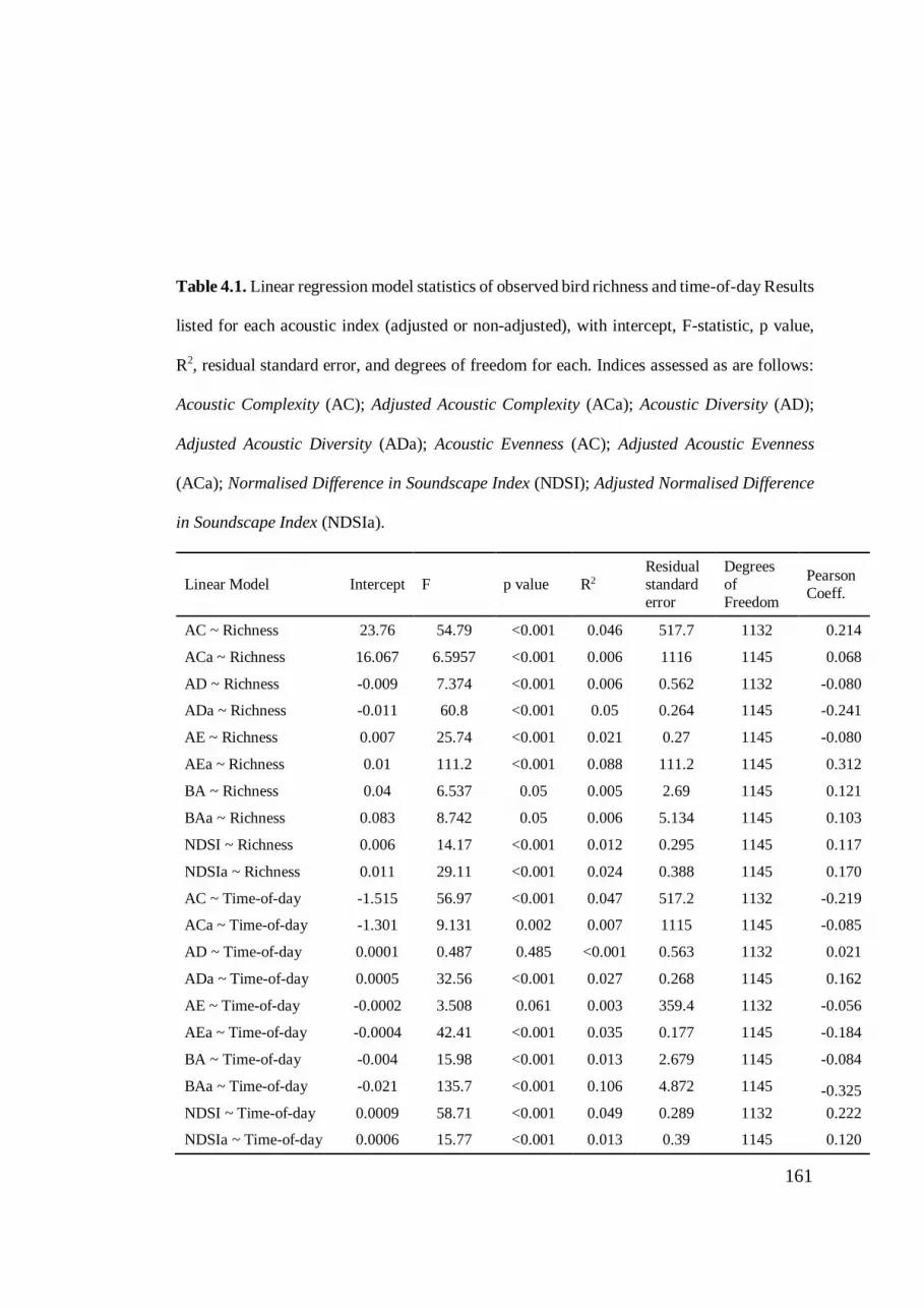
161
Table 4.1. Linear regression model statistics of observed bird richness and time-of-day Results
listed for each acoustic index (adjusted or non-adjusted), with intercept, F-statistic, p value,
R2, residual standard error, and degrees of freedom for each. Indices assessed as are follows:
Acoustic Complexity (AC); Adjusted Acoustic Complexity (ACa); Acoustic Diversity (AD);
Adjusted Acoustic Diversity (ADa); Acoustic Evenness (AC); Adjusted Acoustic Evenness
(ACa); Normalised Difference in Soundscape Index (NDSI); Adjusted Normalised Difference
in Soundscape Index (NDSIa).
Linear Model Intercept F p value R2
Residual
standard
error
Degrees
of
Freedom
Pearson
Coeff.
AC ~ Richness 23.76 54.79 <0.001 0.046 517.7 1132 0.214
ACa ~ Richness 16.067 6.5957 <0.001 0.006 1116 1145 0.068
AD ~ Richness -0.009 7.374 <0.001 0.006 0.562 1132 -0.080
ADa ~ Richness -0.011 60.8 <0.001 0.05 0.264 1145 -0.241
AE ~ Richness 0.007 25.74 <0.001 0.021 0.27 1145 -0.080
AEa ~ Richness 0.01 111.2 <0.001 0.088 111.2 1145 0.312
BA ~ Richness 0.04 6.537 0.05 0.005 2.69 1145 0.121
BAa ~ Richness 0.083 8.742 0.05 0.006 5.134 1145 0.103
NDSI ~ Richness 0.006 14.17 <0.001 0.012 0.295 1145 0.117
NDSIa ~ Richness 0.011 29.11 <0.001 0.024 0.388 1145 0.170
AC ~ Time-of-day -1.515 56.97 <0.001 0.047 517.2 1132 -0.219
ACa ~ Time-of-day -1.301 9.131 0.002 0.007 1115 1145 -0.085
AD ~ Time-of-day 0.0001 0.487 0.485 <0.001 0.563 1132 0.021
ADa ~ Time-of-day 0.0005 32.56 <0.001 0.027 0.268 1145 0.162
AE ~ Time-of-day -0.0002 3.508 0.061 0.003 359.4 1132 -0.056
AEa ~ Time-of-day -0.0004 42.41 <0.001 0.035 0.177 1145 -0.184
BA ~ Time-of-day -0.004 15.98 <0.001 0.013 2.679 1145 -0.084
BAa ~ Time-of-day -0.021 135.7 <0.001 0.106 4.872 1145 -0.325
NDSI ~ Time-of-day 0.0009 58.71 <0.001 0.049 0.289 1132 0.222
NDSIa ~ Time-of-day 0.0006 15.77 <0.001 0.013 0.39 1145 0.120

162
Figure 4.1. Relationships between acoustic indices and observed avian richness.
Observed richness derived from point counts over a landuse gradient in Sabah, Borneo. Each
plot is based on 1,259 recordings from multiple habitat types. The line-of-best-fit is derived

163
from a linear regression model. Shaded areas around the trend lines denote 95% confidence
intervals.
Effects of habitat type
Linear models revealed that the associations between acoustic indices and bird
richness was strongly mediated by habitat type (Table 4.2; Fig S4.1; Fig S4.2).
Differences between habitat types were particularly strong for Acoustic Complexity,
Bioacoustic index and Acoustic Evenness. The effect of habitat type was greater for
adjusted indices than untransformed ones (Table 4.2; Fig. S4.1). We partitioned our
data between the five habitat types in our study (Fig. S4.1) and found that bird diversity
could be predicted by one or more acoustic indices in every habitat type except for oil
palm riparian reserves, where no relationship was found.
Table 4.2. General linear models for each acoustic index in relation to richness, time-
of-day, and habitat types covariates. Intercepts, standard errors and p values are listed for
each parameter. Model AIC and degrees of freedom (DF) are present for each model. For
negative intercepts < signifies values closer to zero. Indices assessed as are follows: Acoustic
Complexity (AC); Adjusted Acoustic Complexity (ACa); Acoustic Diversity (AD); Adjusted
Acoustic Diversity (ADa); Acoustic Evenness (AC); Adjusted Acoustic Evenness (ACa);
Normalised Difference in Soundscape Index (NDSI); Adjusted Normalised Difference in
Soundscape Index (NDSIa).
Model (family) Parameter Intercept p value DF AIC
AC
(Gamma)
observed richness <-0.001 <0.001 1127 17258
Time <0.001 <0.001
logged forest <-0.001 <0.001
riparian forest <-0.001 <0.001

164
riparian oil palm <-0.001 <0.001
riparian reserve <-0.001 0.004
AD (Beta)
observed richness
<-0.001
0.840
1127
1691
Time <-0.001 0.919
logged forest 7.58E-02 0.131
riparian forest 5.20E-01 <0.001
riparian oil palm -0.445 <0.001
riparian reserve 0.251 <0.001
AE
(Beta)
observed richness
4.069
0.071
1127
16166
Time -0.053 0.667
logged forest -67.043 0.024
riparian forest -458.597 <0.001
riparian oil palm 216.904 <0.001
riparian reserve -227.573 <0.001
BA
(Gamma)
observed richness <-0.001 0.694 1118 4584
Time <0.001 0.052
logged forest 0.033 <0.001
riparian forest 0.139 <0.001
riparian oil palm -0.016 0.030
riparian reserve 0.036 <0.001
NDSI
(Beta)
observed richness 0.007 <0.001 1127 304
Time 0.001 <0.001
logged forest -0.012 0.642
riparian forest -0.153 <0.001
riparian oil palm 0.050 0.237
riparian reserve -0.132 <0.001
ACa (Beta)
observed richness 27.767 <0.001 1127 19000
Time -0.643 0.137
logged forest 1048.209 <0.001
riparian forest 1208.966 <0.001
riparian oil palm 739.726 <0.001
riparian reserve 1174.684 <0.001
ADa
(Beta)
observed richness -0.004 <0.001 1127 -25
Time <-0.001 <0.001
logged forest -0.167 <0.001

165
riparian forest 0.084 <0.001
riparian oil palm -0.186 <0.001
riparian reserve 0.097 <0.001
AEa
(Beta)
observed richness -0.004 <0.001 1127 1074
Time <-0.001 <0.001
logged forest 0.102 <0.001
riparian forest -0.097 <0.001
riparian oil palm 0.117 <0.001
riparian reserve -0.081 <0.001
BAa
(Gaussian)
observed richness -0.128 <0.001 1118 6507
Time -0.025 <0.001
logged forest -6.093 <0.001
riparian forest -6.749 <0.001
riparian oil palm -7.716 <0.001
riparian reserve -7.061 <0.001
NDSIa
(Beta)
observed richness 0.012 <0.001 1127 969
Time <0.001 <0.001
logged forest 0.008 0.818
riparian forest -0.149 <0.001
riparian oil palm 0.073 0.195
riparian reserve -0.194 <0.001
Effects of noise-reduction processing
Following our pre-processing adjustments, the strength of association with
point count richness was weaker for Adjusted Acoustic Complexity, but increased for
Adjusted Acoustic Evenness, Adjusted Bioacoustic Index and Adjusted NDSI all
showed relationships of increasing strength (Table 4.1). After adjustment, the effect
of time-of-day was weaker for Adjusted Acoustic Complexity and Adjusted NDSI but
stronger for Adjusted Acoustic Evenness and Adjusted Bioacoustic Index (Table 4.1;
Fig 4.1). We found no associations between indices based on either adjusted or

166
unadjusted recordings with richness or time-of-day in oil palm riparian areas, and these
data were therefore excluded from analysis with estimate richness and canopy height.
Assocations between time-controlled indices, estimated richness and canopy height
After adjustment for time and the exclusion of oil palm riparian data points,
we found no association between estimated richness and Acoustic Complexity time
residuals (R2<0.001, F= 0.01632, p=0.898). Adjusted Acoustic Evenness time
residuals showed a negative relationship with estimated richness, (R2=0.08259,
F=70.76, p<0.001), whereas Adjusted Bioacoustic Index time residuals showed a
strong positive relationship (R2= 0.1581, F=147.6, p<0.001). Acoustic Complexity
time residuals were negatively associated with canopy height (R2=0.07872, F=67.16,
p<0.001), Adjusted Acoustic Evenness time residuals showed no association, while
Adjusted Bioacoustic Index time residuals showed significant positive association
(R2= 0.267, F=286.3, p<0.001). Observed point count richness was associated with
estimated richness (R2=0.08002, F=68.37, p<0.001), but not with canopy height (Fig.
4.2, R2=0.000174, F=0.1368, p=0.712). The strength of association between estimated
richness and canopy height was stronger than for any indices metrics (R2=0.31,
F=367.8, p<0.001), although not markedly different from those revealed by Adjusted
Bioacoustic Index time residuals (Fig. 4.2).

167
Figure 4.2. Time-controlled versions of the three best performing indices in predicting
estimated richness of birds and canopy height. Blue lines denote trendlines, shaded areas mark
168
95% confidence intervals. Data points are different visits (n=1,229), with a maximum of four
visits to any given site (n=356 sites with height and estimated richness data).
Discussion
Our findings demonstrate that acoustic indices, given an appropriate study
design and analytical framework, reflect actual bird diversity patterns across a tropical
forest landscapes, and so could be a viable method of characterising and monitoring
avian biodiversity. However, we also find that in different habitat contexts, non-focal
acoustic signals make highly significant contributions to the overall soundscape and
potentially influence the indices. Although previous studies have sought to assess the
validity of acoustic indices compared to a point count methodology, both in temperate
and tropical regions (Depraetere et al., 2012; Mammides et al., 2017), our study
includes fourfold more spatial replication than previous assessments and does so
across a broad range of habitats and acoustic contexts. As a result, we are able to
provide novel insights into some of the likely reasons for deviations between indices
and point counts, and can make recommendations for how to mitigate factors which
increase discrepancy between acoustic indices and patterns of biodiversity.
Acoustic indices across multiple tropical forest habitats in our study were
associated with observed richness. However, these associations were rather weak and
tended to be mediated by habitat type. Most significantly, none of the indices we tested
showed any significant association with observed species richness in oil palm riparian
areas. Additionally, oil palm riparian areas showed the highest mean levels of
Bioacoustic Index and Acoustic Complexity of any habitat type despite the lowest
levels of observed richness (Fig. S4.1; Fig S4.2). We believe a combination of factors

169
caused a breakdown in any associations between the indices and richness in this
habitat. First, we suspect the influence of human voices in oil palm estates may have
obscured the differences in acoustic complexity driven by bird vocalisations. In urban
environments of the UK, human speech is known to exert a significant bias upon the
same indices quantified in our study (Fairbrass et al., 2017) and it appears likely that
agricultural landscapes, which rely on large numbers of workers (Singana, 2013), have
a similar acoustic profile in this regard. A second factor is that, as in urban areas, avian
communities in oil palm landscapes are depauperate and comprise only a few avian
generalists that occur at almost all sampling points (Chace & Walsh, 2006; Edwards
et al., 2010). In practice, this means limited variation in both the observed number of
species and any acoustic indices and therefore a lower statistically probability of
finding significant associations between the two. This is supported by the fact that we
observed only 3-16 (s.d 2.54) species per count in oil palm, compared to up to 29 (s.d
4.70) species in old-growth forest. For this reason, we removed oil palm riparian sites
from our regression of landscape wide data before comparisons with estimate richness
and canopy height.
Acoustic Complexity was associated with observed richness across the
landscape-wide dataset, but this pattern was not apparent in riparian forests or oil palm
riparian habitats (Fig. 4.1; Fig. S4.2). Riparian forest sites tended to be on steep fast-
running streams where the background noise of running water was significantly louder
than in all other habitats. We suspect this may have undermined the capacity of this
index to detect differences in species richness. Since acoustic complexity is based
upon absolute differences in signal power within each frequency band over time it
should, in theory, account for constant background noise (Pieretti et al., 2011).

170
However, if such noise is sufficiently loud as to drown the signals of bird
vocalisations, this would significantly dampen the variations in signal power over time
and, therefore, reduce the capacity of the index to reflect overall acoustic complexity.
Pre-processing our recordings to produce an adjusted index did not improve the
association levels with observed richness globally, but did increase Adjusted Acoustic
Complexity in riparian forest (with most background noise) relative to other habitat
types (Fig. 4.1).
Across the landscape-wide dataset, we found a weak but significant association
between bioacoustic index and observed richness. However, when broken down to
different habitat types, this pattern was only significant in riparian forest (and not in
old growth, logged forest, riparian reserves or oil palm riparian). A possible
explanation for this pattern is the influence of cicada choruses. Cicadas are common
throughout Bornean rainforests and make a major contribution to the overall
soundscape (Gogala & Riede, 1995). However, cicadas tend to call at constant
frequencies (e.g Gogala & Trilar 2004) and within the frequencies 2 KHz to 8 KHz.
This frequency range is generally regarded as that within which most bird vocalisation
fall (Goller & Riede, 2012) and therefore was used as the limiting bounds in the
development of the bioacoustic index (Boelman et al., 2007). The index calculates the
total spectral energy within this range and does not differentiate between constant-
frequency signals (such as cicada calls) and complex signals (such as most bird songs).
Therefore, a few generalist cicada species calling more frequently could potentially
still result in high index values. Some endothermic species of tropical forest cicada
have been found not to call until certain temperature is reached (Sanborn et al., 1994),
and since old growth forest have been shown to have a greater thermal buffering

171
capacity than logged forests (Frey et al., 2016), it is possible that the onset of certain
species calls is delayed, therefore resulting in a differing level of contribution to the
overall soundscape during the periods we analysed.
Acoustic Evenness decreased with observed bird richness, while previous
studies have shown both positive (Eldrige et al., 2018) and negative (Mammides et
al., 2017) associations. Acoustic Evenness is an entropic index based on overall
evenness between 1 KHz frequency bands (Villanueva-Rivera et al. 2011). Its
interpretation is complex since potentially high values can be reported for signals with
opposing ecological characteristics. As noted by Eldridge et al. (2018), complex
signals with many amplitude modulations have low temporal entropy, but sustained
sounds of consistent frequency show very high temporal entropy. Therefore, we
suspect that acoustic evenness may also have been influenced by the variation and
regularity in cicada calls. This means that more cicada species calling at frequencies
straddling multiple different bands would increase evenness. However, some species
of cicada call at narrow, constant frequency bands (e.g Sanborn, 1997), if these were
to fall within a particular 1 kHz bound assessed by the index, this would reduce
evenness.
Although some studies have sought to control for cicada choruses by excluding
them (Towsey et al., 2013), the uneven temporal distribution of such signals means
excluding them would add new biases based the time of sampling. Previous studies
have also found that temporal differences in cicada chorus introduced bias in entropic
indices, which resulted in higher index values in degraded than intact tropical forest
(Sueur et al., 2008). The loud insect chorus characteristic of Bornean rainforests has
also been suspected of resulting in ‘jamming avoidance’, whereby some taxa sing less

172
frequently during the loudest choruses of others (Reide, 1997). This could in theory
also affect the acoustic evenness index, since complex signals such as birdsong may
be inhibited by cicada calls. Therefore, understanding how changes in cicada choruses
effect acoustic indices is therefore a major research priority for optimising their utility
in tropical forests.
Our results showed a weak positive association between NDSI and observed
richness across all habitats. However, the perceived influence of anthropogenic sound
was highly heterogeneous when point counts were conducted. Whilst oil palm riparian
areas undoubtedly had a greater proportion of anthropogenic sounds, many logged
forest sites were still undergoing salvage logging nearby to where our counts were
conducted. This resulted in distant chainsaw and vehicle sounds being relatively
common within our recordings. A high proportion of old growth sites were influence
by the sounds of vehicles, leaf-blowers and road construction nearby.
Bioacoustic index values were greater in old growth forest, followed by logged
forests, then riparian reserves and riparian forest (Fig. 4.1). This pattern (excluding for
oil palm) mirrored the aggregated habitat richness findings from our previous analysis
of the landscape (Chapter 2; Mitchell et al., 2018), as well as a large literature showing
that old growth forests support more bird species than logged forests (Edwards et al.,
2014) or isolated fragments (Edwards et al., 2010). Associations between bioacoustic
index values and observed richness from individual point counts may have been weak
due to the observed richness being a poor reflection of actual avian richness patterns.
This is because the majority of species in tropical forest are rather uncommon, with
some not even calling every day (Robinson et al. 2018).

173
Incomplete sampling of some species due to a failure in detection contributes
to the discrepancy between acoustic indices and richness patterns. This is supported
by the negative relationships found between several indices and time-of-day (Table
4.1). This idea is supported by two patterns we observed. First, associations between
bioacoustics index and estimate richness (controlled for detection probability), were
far higher than those with observed richness (Fig. 4.3). Second the overall avian chorus
(and hence the probability of a given species vocalising) decreased with time after
dawn (Table 4.1). Similar patterns have been noted in several previous studies
(Wimmer et al., 2013). Since observed richness from point counts can be based on
upward of 95% aural encounters in tropical forests (Robinson et al., 2018), this metric
also decreases with time after dawn. However, the effect of time upon acoustic indices
and observed richness is not the same, since point counts do not rely solely upon
vocalisations. This means that the differing effects of time upon the two metrics
introduces a source of bias. We found that associations between indices and observed
richness within our landscape-level dataset improved when we used time-controlled
residuals for both. We therefore recommend this step for any sampling designs that
base their acoustic indices upon samples from different times of day. However, for
extended or constant autonomous recordings, there are alternatives to this approach,
such as using sampling designs which validate recordings based on one minute
samples, taken at random or via a stratified sampling approach depending on the
results for particular indices (Wimmer et al., 2013).
Pre-processing our recordings to remove frequencies outside of our focal range
of 800 - 10,000 kHz (the range within which tropical bird vocalisation fall), as well as
removing 12 dB of background noise using a manually set noise profile, resulted in

174
improved associations between indices and observed richness. We referred to these as
adjusted indices for simplicity, although the actual process involved editing the
recording themselves before re-running the same computations for calculating
acoustic metrics. Adjusted indices, showed stronger associations with observed
richness for evenness, NDSI and Bioacoustics Index (Table 4.1; Fig. 4.1; Fig. 4.2).
Notably, Adjusted Bioacoustic Index values increased significantly in riparian habitats
(riparian forest where the sounds of running water were strongest and riparian reserves
where they were of variable intensity) relative to those without background noise. This
supports our hypothesis that high level of geophonic background noise ‘drown out’
bird vocalisations in these habitats.
We also assessed the performance of the acoustic indices most associated with
observed richness (Acoustic Complexity time residuals, Adjusted Acoustic Evenness
time residuals, Adjusted Bioacoustic Index time residuals) against estimated richness
(Fig. 4.2). Observed richness time residuals (Point count residuals; the total number
of species encountered during each point count), does not account for imperfect
detection (i.e. the majority of species are not heard or seen during the 15-minute period
of a single point count). Whilst observed richness is appropriate for validating the link
between the species heard by observer during points and resulting representation of
this via a given acoustic index, it is not necessarily useful for measuring true patterns
of avian richness across landscapes. In fact, we found no relationship between
observed richness from individual point counts and canopy height; an environmental
variable which has been found to strongly influence richness in Bornean tropical
forests (Cleary et al., 2005). Bioacoustic Index time residuals were the most strongly
associated metric with estimated richness (R2 = 0.15), and was more closely linked

175
than observed richness and estimated richness (R2 = 0.08). This suggests that
Bioacoustic Index time residuals could therefore be used as a viable proxy measure of
biodiversity across tropical forest landscapes.
Although previous studies have demonstrated that acoustic indices are capable of
measuring changes in species richness changes associated with changes in landscape
configuration (Fuller et al., 2015), their ability to reflect patterns associated with
environmental or structural gradients across multiple habitats remains uncertain
(Farina & Pieretti, 2014). In fact, the latter study is the only one to date which has
assessed the relationship between vegetation structure and acoustic indices and even
in this case, indices were broken metrics down into smaller categorical variables,
rather than using a continuous gradient approach. The way in which associations
between vegetation metrics and acoustic indices is mediated by species richness is also
still poorly understood and may be contingent upon a number of other factors such as
bird community composition or vegetation structure (Boelman et al., 2007). For
acoustic indices to be of similar utility to existing methodologies they must be able to
reflect biological patterns at a comparable level to conventional methodologies.
Comparisons between Bioacoustic Index time residuals and canopy height (R2 = 0.26),
showed a similar level of association to that of estimated richness and canopy height
(R2 = 0.31). This demonstrates that Bioacoustic Index time residuals t performs at a
similar level to establish advanced modelling techniques reflected patterns of
biodiversity associated with an environmental gradient. Since much biodiversity
assessment and conservation research is concerned with identifying the effects of
environmental and human-mediated changes to the landscape, the fact that acoustic

176
indices are able to capture the effects of such environmental gradients supports their
deployment more widely as a method of assessing biodiversity.
Soundscape indices can be used to reflect patterns of biodiversity across varied
landscapes with significantly different community assemblages and different levels of
species richness. By following these steps we were able to increase the associations
between acoustic indices and richness from very weak (R2 of 0.02 for Acoustic
Evenness as the strongest initial association), to better than raw data from conventional
point counts and comparable those of current best-available modelling approaches (R2
of 0.26 for Bioacoustic Index time residuals).
With correct deployment and analysis, such indices are capable of capturing
variation in ecological communities associated with environmental gradients such as
differences in vegetation structure. The utility of acoustic indices provides efficient
ways of quantifying biodiversity, without the need for expert validation, and means
that such methods are an excellent tool for conservation and in particular rapid
biodiversity assessments, especially in the context of limited resources and an ever-
growing number of environmental crises. Future advances in acoustic approaches,
particularly those based on deep-learning, have the potential accurately identifying
individual species and show highly promising potential for assessing and monitoring
tropical forests (Burivalova et al., 2019). However, at present the main application of
these indices rests with quantifying community-level acoustics, and misses vast
information at the species level, which can inform which species are dominant and
rare, and hence of a conservation priority.

177
Supplemental Materials
Figure S 4.1. Violin plots with embedded boxplots for adjusted indices. Acoustic Acoustic
Complexity, Adjusted Acoustic Complexity and Acoustic Evenness, Adjusted Acoustic
Evenness, Bioacoustic Index, Adjusted Bioacoustic Index, NDSI and Adjusted NDSI in each
habitat: Old growth; Logged forest; Riparian forest; Riparian reserve and Riparian oil palm.

178
Figure S 4.2. Regressions of the best performing indices against observed species richness.
Acoustic Complexity; Adjusted Acoustic Evenness; Adjusted Bioacoustic Index and Adjusted
NDSI against Point count richness for each habitat: Old growth; Logged growth; Riparian

179
forest; Riparian reserves and Riparian oil palm. R2, F statistic and p values of each relationship
are listed at the top right of each respective panel.

180
Acknowledgements
This study was funded by the UK Natural Environment Research Council (NERC)
(NE/K016407/1; http://lombok.hmtf.info/ and http://bali.hmtf.info; NE/K016377/1),
and a Newton-Ungku Omar Fund grant from the British Council and Malaysia
Industry-Group for High Technology (MIGHT) (216433953). SLM was supported by
a PhD scholarship jointly funded by University of Kent and NERC. We thank the
Sabah Biodiversity Council, Sabah Forest Department, Yayasan Sabah, Sime Darby,
Benta Wawasan, Sabah Softwoods and Innoprise Foundation for permitting site
access. We are grateful to Unding Jami and the LOMBOK research assistant team for
their field assistance, and Suzan Benedick, Joseph Tobias and Ryan Gray for
facilitating fieldwork.
References
Alquezar, R.D. & Machado, R.B. (2015) Comparisons between autonomous acoustic
recordings and avian point counts in open woodland savanna. The Wilson
Journal of Ornithology, 127, 712–723.
Arnold, V. Using Audacity for analysing and editing recordings of bird voices.
https://www.dropbox.com/s/cn56iuw4gszmlx5/usingaudacity.pdf?dl=0
Asner, G.P., Brodrick, P.G., Philipson, C., Vaughn, N.R., Martin, R.E., Knapp, D.E.,
Heckler, J., Evans, L.J., Jucker, T., Goossens, B., Stark, D.J., Reynolds, G., Ong,
R., Renneboog, N., Kugan, F. & Coomes, D.A. (2018) Mapped above ground
carbon stocks to advance forest conservation and recovery in Malaysian Borneo.
Biological Conservation, 217, 289–310.

181
Barlow, J., Mestre, L.A.M., Gardner, T.A. & Peres, C.A. (2007) The value of primary,
secondary and plantation forests for Amazonian birds. Biological Conservation,
136, 212–231.
Boelman, N.T., Asner, G.P., Hart, P.J. & Martin, R.E. (2007) Multi-trophic invasion
resistance in Hawaii: Bioacoustics, field surveys, and airborne remote sensing.
Ecological Applications, 17, 2137–2144.
Burivalova, Z., Game, E.T. & Butler, R.A. (2019) The sound of a tropical forest.
Science, 363, 28–29.
Bustamante, M.M.C., Roitman, I., Aide, T.M., Alencar, A., Anderson, L.O., Aragão,
L., Asner, G.P., Barlow, J., Berenguer, E., Chambers, J., Costa, M.H., Fanin, T.,
Ferreira, L.G., Ferreira, J., Keller, M., Magnusson, W.E., Morales-Barquero, L.,
Morton, D., Ometto, J.P.H.B., Palace, M., Peres, C.A., Silvério, D., Trumbore,
S. & Vieira, I.C.G. (2016) Toward an integrated monitoring framework to assess
the effects of tropical forest degradation and recovery on carbon stocks and
biodiversity. Global Change Biology, 22, 92–109.
Chace, J.F. & Walsh, J.J. (2006) Urban effects on native avifauna: A review.
Landscape and Urban Planning, 74, 46–69.
Cleary, D.F.R., Genner, M.J., Boyle, T.J.B., Setyawati, T., Angraeti, C.D. & Menken,
S.B.J. (2005) Associations of bird species richness and community composition
with local and landscape-scale environmental factors in Borneo. Landscape
Ecology, 20, 989–1001.
182
Darras, K., Batáry, P., Furnas, B., Celis-Murillo, A., Van Wilgenburg, S.L., Mulyani,
Y.A. & Tscharntke, T. (2018) Comparing the sampling performance of sound
recorders versus point counts in bird surveys: A meta-analysis. Journal of
Applied Ecology, 55, 2575–2586.
Davies, A.B. & Asner, G.P. (2014) Advances in animal ecology from 3D-LiDAR
ecosystem mapping. Trends in Ecology and Evolution, 29, 681–691.
Delignette-Muller, M.L. & Dutang, C. (2015) An {R} Package for Fitting
Distributions. Journal of Statistical Software, 64, 1–34.
Depraetere, M., Pavoine, S., Jiguet, F., Gasc, A., Duvail, S. & Sueur, J. (2012)
Monitoring animal diversity using acoustic indices: Implementation in a
temperate woodland. Ecological Indicators, 13, 46–54.
Edwards, D.P., Gilroy, J.J., Woodcock, P., Edwards, F.A., Larsen, T.H., Andrews,
D.J.R., Derhé, M.A., Docherty, T.D.S., Hsu, W.W., Mitchell, S.L., Ota, T.,
Williams, L.J., Laurance, W.F., Hamer, K.C. & Wilcove, D.S. (2014) Land-
sharing versus land-sparing logging: Reconciling timber extraction with
biodiversity conservation. Global Change Biology, 20, 183–191.
Edwards, D.P., Hodgson, J.A., Hamer, K.C., Mitchell, S.L., Ahmad, A.H., Cornell,
S.J. & Wilcove, D.S. (2010) Wildlife-friendly oil palm plantations fail to protect
biodiversity effectively. Conservation Letters, 3, 236–242.
Eldridge, A., Guyot, P., Moscoso, P., Johnston, A., Eyre-Walker, Y. & Peck, M.
(2018) Sounding out ecoacoustic metrics: Avian species richness is predicted by

183
acoustic indices in temperate but not tropical habitats. Ecological Indicators, 95,
939–952.
Ewers, R.M., Didham, R.K., Fahrig, L., Ferraz, G., Hector, a., Holt, R.D., Kapos, V.,
Reynolds, G., Sinun, W., Snaddon, J.L. & Turner, E.C. (2011) A large-scale
forest fragmentation experiment: the Stability of Altered Forest Ecosystems
Project. Philosophical Transactions of the Royal Society B: Biological Sciences,
366, 3292–3302.
Fairbrass, A.J., Rennett, P., Williams, C., Titheridge, H. & Jones, K.E. (2017) Biases
of acoustic indices measuring biodiversity in urban areas. Ecological Indicators,
83, 169–177.
Farina, A. & Pieretti, N. (2014) Sonic environment and vegetation structure: A
methodological approach for a soundscape analysis of a Mediterranean maqui.
Ecological Informatics, 21, 120–132.
Frey, S.J.K., Hadley, A.S., Johnson, S.L., Schulze, M., Jones, J.A. & Betts, M.G.
(2016) Spatial models reveal the microclimatic buffering capacity of old-growth
forests. Science Advances, 2.
Fuller, S., Axel, A.C., Tucker, D. & Gage, S.H. (2015) Connecting soundscape to
landscape: Which acoustic index best describes landscape configuration?
Ecological Indicators, 58, 207–215.
Gage, S.H., Napoletano, B.M. & Cooper, M.C. (2001) Assessment of ecosystem
biodiversity by acoustic diversity indices. The Journal of the Acoustical Society
of America, 109, 2430–2430.

184
Gardner, T. A., Barlow, J., Araujo, I. S., Ávila‐Pires, T. C., Bonaldo, A. B., Costa, J.
E., ... & Hoogmoed, M. S. (2008). The cost‐effectiveness of biodiversity surveys
in tropical forests. Ecology Letters, 11(2), 139-150.
Gasc, A., Sueur, J., Jiguet, F., Devictor, V., Grandcolas, P., Burrow, C., Depraetere,
M. & Pavoine, S. (2013) Assessing biodiversity with sound: Do acoustic diversity
indices reflect phylogenetic and functional diversities of bird communities?
Ecological Indicators, 25, 279–287.
Gasc, A., Francomano, D., Dunning, J.B. & Pijanowski, B.C. (2017) Future directions
for soundscape ecology: The importance of ornithological contributions. The
Auk, 134, 215–228.
Gogala, M. & Riede, K. (1995) Time sharing of song activity by cicadas in Temengor
forest reserve, Hulu Perak, and in Sabah, Malaysia. Marayan Nature Journal, 48,
297–305.
Goller, F., & Riede, T. (2012). Integrative physiology of fundamental frequency
control in birds. Journal of Physiology-Paris, 107(3), 230-242.Guo, X., Coops,
N.C., Tompalski, P., Nielsen, S.E., Bater, C.W. & John Stadt, J. (2017) Regional
mapping of vegetation structure for biodiversity monitoring using airborne lidar
data. Ecological Informatics, 38, 50–61.
Harris, S.A., Shears, N.T. & Radford, C.A. (2016) Ecoacoustic indices as proxies for
biodiversity on temperate reefs. Methods in Ecology and Evolution, 7, 713–724.

185
Izaguirre, M. I. R., Ramírez-Alán, O., & De la O Castro, J. (2018). Acoustic indices
applied to biodiversity monitoring in a Costa Rica dry tropical forest. Journal of
Ecoacoustics, 2 .
Kasten, E.P., Gage, S.H., Fox, J. & Joo, W. (2012) The remote environmental
assessment laboratory’s acoustic library: An archive for studying soundscape
ecology. Ecological Informatics, 12, 50–67.
Kottege, N., Jurdak, R., Kroon, F. & Jones, D. (2015) Automated detection of
broadband clicks of freshwater fish using spectro-temporal features. The Journal
of the Acoustical Society of America, 137, 2502–2511.
Lee, B. P. Y., Davies, Z. G., & Struebig, M. J. (2017). Smoke pollution disrupted
biodiversity during the 2015 El Niño fires in Southeast Asia. Environmental
Research Letters, 12(9), 094022.
Lewandowski, A.S., Noss, R.F. & Parsons, D.R. (2010) The effectiveness of surrogate
taxa for the representation of biodiversity. Conservation Biology, 24, 1367–1377.
Machado, R.B., Aguiar, L. & Jones, G. (2017) Do acoustic indices reflect the
characteristics of bird communities in the savannas of Central Brazil? Landscape
and Urban Planning, 162, 36–43.
Mammides, C., Goodale, E., Dayananda, S.K., Kang, L. & Chen, J. (2017) Do acoustic
indices correlate with bird diversity? Insights from two biodiverse regions in
Yunnan Province, south China. Ecological Indicators, 82, 470–477.

186
Mitchell, S.L., Edwards, D.P., Bernard, H., Coomes, D., Jucker, T., Davies, Z.G. &
Struebig, M.J. (2018) Riparian reserves help protect forest bird communities in
oil palm dominated landscapes. Journal of Applied Ecology, 55, 2744–2755.
Pettoretti, N., Safi, K. and Turner, W. (2014) Satellite remote sensing, biodiversity
research and conservation of the future.Philosophical transactions of the Royal
Society of London. Series B, Biological sciences, 369.
Pieretti, N., Farina, A. & Morri, D. (2011) A new methodology to infer the singing
activity of an avian community : The Acoustic Complexity Index (ACI).
Ecological Indicators, 11, 868–873.
Pijanowski, B.C., Villanueva-Rivera, L.J., Dumyahn, S.L., Farina, A., Krause, B.L.,
Napoletano, B.M., Gage, S.H. & Pieretti, N. (2011) Soundscape Ecology: The
Science of Sound in the Landscape. BioScience, 61, 203–216.
Pijanowski, B.C., Villanueva-Rivera, L.J., Dumyahn, S.L., Farina, A., Krause, B.L.,
Napoletano, B.M., Gage, S.H. & Pieretti, N. (2011) Soundscape Ecology: The
Science of Sound in the Landscape. BioScience, 61, 203–216.
Presern, J., Gogala, M. & Trilar, T. (2004) Comparisons of Dundubia Vaginata
(Auchenorrhyncha: Cicadoeidae) sones from Borneo and Penninsular Malayia.
Acta Entormologica Slovenia, 12, 293–248.
Retamosa Izaguirre, M.I., Ramírez-alán, O. & Castro, J.D.O. (2018) Acoustic indices
applied to biodiversity monitoring in a Costa Rica dry tropical forest. Journal of
ecoacoustics, 2, 1–21.

187
Riede, K. (1997) Bioacoustic diversity and resource partitioning in tropical
callingcommunities. Tropical biodiversity and systematics: Proceedings of the
International Symposium on Biodiversity and Systematics in Tropical
Ecosystems, 1, 275–280.
Ripple, W.J., Wolf, C., Newsome, T.M., Galetti, M., Alamgir, M., Crist, E.,
Mahmoud, M.I. & Laurance, W.F. (2017) World Scientists’ Warning to
Humanity: A Second Notice. BioScience, 67, 1026–1028.
Royle, J.A. & Kery, M. (2015) A Bayesian state-space formulation of dynamic
occupancy models. Ecology, 88, 1813–1823.
Rockström, J., Steffen, W., Noone, K., Persson, Å., Chapin III, F.S., Lambin, E.,
Lenton, T.M., Scheffer, M., Folke, C., Schellnhuber, H.J. and Nykvist, B., 2009.
Planetary boundaries: exploring the safe operating space for humanity. Ecology
and Society, 14(2).
Sanborn, A.F. (1997) Body temperature and the acoustic behavior of the cicada
Tibicen winnemanna (Homoptera: Cicadidae). Journal of Insect Behavior, 10,
257–264.
Sanborn, A.F., Heath, M.S., Heath, J.E. & Noriega, F.G. (1995) Diurnal activity,
temperature responses and endothermy in three South American cicadas
(Homoptera: Cicadidae: Dorisiana bonaerensis, Quesada gigas and Fidicina
mannifera). Journal of Thermal Biology, 20, 451–460.

188
Sinaga, H. (2013) Employment and Income of Workers on Indonesian Oil Palm
Plantations: Food Crisis at the Micro Level Future of Food: Journal on Food,
Agriculture and Society, 1, 64–78.
Sueur, J., Aubin, T. & Simonis, C. (2008) Equipment review: Seewave, a free modular
tool for sound analysis and synthesis. Bioacoustics, 18, 213–226.
Sueur, J., Farina, A., Gasc, A., Pieretti, N. & Pavoine, S. (2014) Acoustic Indices for
Biodiversity Assessment and Landscape Investigation. Acta Acustica united with
Acustica, 100, 772–781.
Sueur, J., Pavoine, S., Hamerlynck, O. & Duvail, S. (2008) Rapid acoustic survey for
biodiversity appraisal. PLoS ONE, 3.
Taft, O. W., Haig, S. M., & Kiilsgaard, C. (2003). Use of radar remote sensing
(RADARSAT) to map winter wetland habitat for shorebirds in an agricultural
landscape. Environmental Management, 32(2), 268-281.
Towsey, M., Wimmer, J., Williamson, I. & Roe, P. (2014) The use of acoustic indices
to determine avian species richness in audio-recordings of the environment.
Ecological Informatics, 21, 110–119.
Valentini, A., Taberlet, P., Miaud, C., Civade, R., Herder, J., Thomsen, P.F.,
Bellemain, E., Besnard, A., Coissac, E., Boyer, F., Gaboriaud, C., Jean, P.,
Poulet, N., Roset, N., Copp, G.H., Geniez, P., Pont, D., Argillier, C., Baudoin,
J.M., Peroux, T., Crivelli, A.J., Olivier, A., Acqueberge, M., Le Brun, M., Møller,
P.R., Willerslev, E. & Dejean, T. (2016) Next-generation monitoring of aquatic

189
biodiversity using environmental DNA metabarcoding. Molecular Ecology, 25,
929–942.
Villanueva-Rivera, L.J., Pijanowski, B.C., Doucette, J. & Pekin, B. (2011) A primer
of acoustic analysis for landscape ecologists. Landscape Ecology, 26, 1233–
1246.
Villard, L., Le Toan, T., Tang Minh, D.H., Mermoz, S. & Bouvet, A. (2016) Forest
Biomass From Radar Remote Sensing. Land Surface Remote Sensing in
Agriculture and Forest, 363–425.
Vitousek, P.M., Aber, J.D., Howarth, R.W., Likens, G.E., Matson, P.A., Schidler,
D.W., Schlesinger, W.H. & Tilman, D.G. (1997) Multi-Trophic Invasion
Resistance in Hawaii: Bioacoustics, Field Surveys, and Airborne Remote
Sensing. Ecological Society of America, 7, 737–750.
Walker, B., Hansen, J., Corell, R.W., Fabry, V.J., Karlberg, L., Falkenmark, M.,
Svedin, U., Snyder, P.K., Costanza, R., Rodhe, H., Sörlin, S., Leeuw, S. van Der,
Hughes, T., Wit, C.A. de, Nykvist, B., Schellnhuber, H.J., Folke, C., Scheffer,
M., Lenton, T.M., Lambin, E., Chapin, F.S.I.I.I., Persson, Å., Noone, K., Steffen,
W., Rockström, J., Liverman, D., Richardson, K., Crutzen, P. & Foley, J. (2009)
Planetary Boundaries: Exploring the Safe Operating Space for Humanity.
Ecology and Society, 14, 32.
Wimmer, J., Towsey, M., Roe, P. & Williamson, I. (2013) Sampling environmental
acoustic recordings to de- termine species richness. Ecological Applications, 23,
1419–1428.

190

191
Discussion
Throughout this thesis I have explored the impacts of tropical forest degradation and
loss on biodiversity across a landscape gradient from old growth forests, to agricultural
plantations. The application of novel technological and statistical approaches has
yielded two important insights. First, I have been able to address unanswered questions
regarding biodiversity responses to landuse change including thresholds of response
to habitat modification for many species. Second, I have been able to demonstrate the
applicability of these novel approaches in the context of practical ecological questions,
and give policy-relevant recommendations as a result.
The application of LiDAR technologies in biodiversity monitoring
In Chapter 1 I revealed the biodiversity value of riparian reserves in oil palm
landscapes, using birds as surrogate taxa. To examining the relationship between
riparian reserve width, carbon density and species richness, I utilised LiDAR derived
data to gain insight that would not otherwise have been possible, and suggest practical
recommendations. I recommended that reserves would become more optimal habitat
for birds by increasing riparian vegetation from 30 to 40 m on each side of river, but
that reserves still do not reach equivalent bird species richness until forest quality is
improved (exceeding 60 tonnes of carbon per hectare in tree biomass). This appraisal
was made possible by being able to use LiDAR data to measure both riparian width
and carbon density. Although direct measures of river and riparian zone width could
be undertaken in the field with measure tapes or rangefinders, my early attempts to do
this proved futile given the terrain and difficulty in surveying a sufficiently
192
representative cross-section of the river and reserve. Likewise, the implementation of
on-the-ground vegetation plots in many areas of the landscape would have been
prohibitively time consuming. In comparison, ground-truthing of LiDAR plots was
only undertaken at a subset of sample points and as a collaborative effort out in by
multiple members of the Stability of Altered Forest Ecosystem staff as well as
members of the LOMBOK consortium (Jucker et al., 2018).
There has been a huge proliferation in remote sensing technologies in recent
years. In 2001 LANDSAT imagery was virtually the only publically available earth-
observation dataset (Pimm et al., 2015). However, by 2008 at least 19 different earth
observation satellites were operating (Gillespie et al., 2008) and 268 additional
missions were in the planning stage by 2012 (Selva & Krejci, 2012). Since 2000 the
number of civilian missions has grown exponentially, with the spatial resolution of
data also continuingly increasing (Belward & Skoien, 2015) As well as offering
potentially new ways of mapping land cover (including in three dimensions), perhaps
the most fundamental gain for biodiversity monitoring has been the increased
efficiency and reduced cost of collecting data for large areas. As a result, the spatial
scales on which biodiversity is assessed have expanded significantly, both in the
context of single study landscapes, and meta-analytic global analyses. Remote sensing
also allows the assessment of vegetation in areas which may be inaccessible due to
terrain (e.g Avisse et al., 2017) or security issues.
LiDAR data were integral to the research presented in each data chapter.
Chapter 3 in particular assessed species occupancy responses against the high
resolution measures of forest structure derived from the LiDAR, including the overall
density of vegetation and the vertical skew in the distribution of that density. These

193
covariates would be difficult to derive from conventional reflectance-only remote
sensing technologies, since they necessarily require hyperspectral signals that can
penetrate through the top layers of canopy in order to map 3-dimensional vegetation
structure. The application of LiDAR technologies to studies in other parts of the
tropics could fundamentally change our understanding of how biodiversity is
distributed from two dimensions to three.
Sabah now has near state-wide LiDAR coverage thanks to a recent aerial
survey mission led by the Carnegie Airborne Observatory (Asner et al., 2018), which
potentially allows for patterns of biodiversity to be modelled on a large scale in
relation to the vegetation and landscape configuration data captured from these flights.
The Sabah state government also has ambitions to increase its protected area network
from 21% to 30% percent of the total land area. There is therefore an opportunity for
modelling studies such as those I present in Chapter 3 to help inform state-wide
conservation policy. The availability and applicability of LiDAR technology globally
also looks set to expand. December 2018 marked the launch of the NASA Global
Ecosystem Dynamics Investigation (GEDI) LiDAR mission - a global, satellite-based
assessment of vegetation (Saarela et al., 2018). Deploying such assessments globally
offers a genuine step change in the way conservation prioritisations can be done, and
in particular could help discern the relative biodiversity value of different landuse
intensities in human modified agricultural systems.
The ability to use LiDAR to define structural niches for highly specialised
species is already proving useful in defining specific management plans. For example,
LiDAR assessments have helped to define the habitat structure requirements of Red-
cockaded Woodpecker in the Southern United States (Smart et al., 2012). In another

194
study of the same species, researchers were able to identify lower and upper thresholds
for densities of pines, basal area of pines, tree diameter at breast height, hardwood
canopy cover and basal area of hardwoods using ground-based LiDAR assessments
which have informed federal management plans in the United States (Garabedian et
al., 2017). LiDAR has also been used to determine habitat association in studies on
wood-mice (Jaime-Gonzalez et al., 2017), dormice (Goodwin et al., 2018); bats
(Froidevaux et al., 2016) and birds in tropical forests (Flaspohler et al., 2010),
temperate woodland and agricultural landscapes (Bradbury et al., 2015). The
trajectory of increase coverage and affordability of these technologies mean that
including a third dimension in appraisals of habitat structure (particularly in contexts
such as tropical forest where this is highly relevant), could eventually become the
default approach to species-habitat studies.
Challenges in occupancy modelling to monitor rare species
Tropical forest bird communities often contain large numbers of species that are
difficult to detect (Robinson et al., 2018). It has been noted previously that some
tropical bird taxa are both visually cryptic and rarely vocalise. For example, radio-
telemetry tracking of a Variegated Antpitta (Grallaria varia) documented instances of
singing at just two of 68 locations within its home range (Jirinecet al. 2018; Robinson
et al., 2018). We noted that this was also the case for several species with our study
system. For example Giant Pitta (Hydrornis caeruleus) was only noted from point
counts on three occasions during five field seasons, despite the observers being highly
familiar with its distinctive vocalisation.

195
Additionally, a number of species in our study areas were mostly documented
from distances of greater than 50 m. These encounters were removed from our
occupancy modelling assessments, since we focussed on examining habitat
associations within a 50 m radius of each point count station and points were separated
by 180 m. These species tended to be quite vocal, but occurred at low-densities, and
were not adequately assessed using a conventional point count methodology over
limited-distances. Perhaps the most prominent example of this is that the far-carrying
call of the Critically Endangered (IUCN, 2019) Helmeted Hornbill (Rhinoplax vigil),
which was noted on 72 occasions, though only six of these were from within 50 m.
Robinson et al. (2018) recommend the approach we adopted, of using unlimited
distance surveys and then truncating data later. However, the advocated technique of
using species-specific distance histograms to inform this approach is not possible
when attempting to optimise sampling methods for an entire community and avoid
including communities of adjacent habitats within the radius of point counts,
particularly in the context of riparian reserves and fragments.
Southeast Asia, principally Indonesia, is also suffering a crisis in songbird
trade. Analysis by Symes et al. (2018) suggests exploitation for wildlife trade has
driven dramatic declines in many species within the region. This has occurred to such
an extent that some species have already declined to a point where they are no longer
easily available at songbird markets and new species are being exploited in a cascade
of demand (Symes et al., 2018). Although cultural factors make wild bird trade a much
more significant factor in Indonesia than Malaysia, several species have declined as a
result of exploitation here too, most notably Helmeted Hornbill Rhinoplax vigil
(Beastall et al., 2016), White-crowned Shama Copsychus barbouri and Straw-headed

196
Bulbul Pycnonotus zeylanicus (Bergin et al., 2018). Indeed the absence of the latter
from areas much of our study areas has been attributed to illegal trapping (Sheldon et
al., 2009.). Forest loss, increased infrastructure for agriculture and fragmentation has
also further increased the problem of illegal bird trapping and hunt, since it results
greater accessibility to ever higher proportions of remnant forests (Symes et al., 2018).
In order to apply a hierarchical modelling approach to these communities some
standardisation of the data is required. For example, in Chapter 3, I excluded species
that had been recorded on fewer than four occasions from the dataset completely, since
trail runs of the modelling approach demonstrated these species to simply follow
community-average trends in responses to environmental variation. The structure of
Bayesian occupancy models mean that data are aggregated at the community level and
this informs species-specific parameter estimates, therefore moving them toward the
community mean (Broms et al., 2016). This remains a potential caveat for some of the
rarer species remaining in the model. Defining specific thresholds for species trait
groups required there be sufficient number of species in each group. On the other hand,
including species based on too few observations would increase the representation of
the community mean hyper-parameters from which they borrow power, and therefore
potentially obscure the differing responses of different trait groups.
The models applied in Chapter 3 did not account for the influence of transects
beyond differences in the five environmental variable we included. I explored the
inclusion of a random factor variable for each of the 33 transects associated with
detection probabilities. However, this increased the size of the model an order of
magnitude, to the extent that even when running on the entire capacity of the
supercluster server at the University of Kent, the analysis exceeded the active memory

197
limits. This demonstrates that there are still some computational impediments for
undertaking complex Bayesian models on very large ecological datasets such as the
one I collected. However, increases in computer processing power are likely to
continue, which should allow the introduction of more powerful models.
The application of bioacoustic approaches to biodiversity monitoring
The development of sophisticated and relatively inexpensive sound recorders in recent
years has opened up new avenues of ecological research. Acoustic approaches to
measure and monitor biodiversity have been undertaken in environments as diverse as
freshwater lakes and coral reefs (Lindseth & Lobel, 2018) and tropical forests
(Burivalova et al., 2018). In particular, algorithms which characterise the spectral
energy or acoustic complexity of recordings and express them as single indexed values
have been shown to be associated with to biodiversity patterns in many contexts
(Buxton et al., 2018). However, the utility of theses methods for assessing biodiversity
on larger scales relies on them being generalisable across multiple habitats, and in a
number of scenarios these indices are not associated with biodiversity as measured by
traditional means. Chapter 4 focussed on ways to optimise such acoustic approaches
and improve their performance in landuse change studies applied across a broad
environmental gradient. I found that the four indices applied typically became more
congruent with species richness when processed for noise reduction and when I
controlled for the effects of time in analyses. Based upon my findings, I offer a series
of recommendations for future soundscape analyses that aim to characterise
biodiversity patterns in tropical habitats:

198
1) Agriculturally intensive environments cannot be adequately compared using
the indices I assessed at present, since these indices are currently unable to
separate the influences of human sounds from signals generated by wildlife.
2) The ability of acoustic indices to act as proxies for biodiversity may be
compromised in habitats with strong geophonic influences, such as fast
flowing water. I demonstrate that the use of proprietary noise reduction
functions software from the free software Audacity (1999-2013 Audacity
Team; SourceForge.net), to transform recordings (Chapter 3) helps minimise
this influence. Application of this transformation improves the performance of
three out of four indices in all habitats, albeit to a small degree.
3) In tropical forests there is potentially a strong influence of cicada choruses
upon acoustic indices. Further study into the specific effects of cicada and
insect noise more generally upon the outcomes of acoustic indices is required.
Assessment of how call diversity and regularity in insect taxa are associated
with broader patterns of biodiversity will help in the appropriate deployment
of existing acoustic indices as well as development of new metrics. Ideally, to
control for potential discrepancies introduced by cicadas, future studies should
attempt to quantify the regularity and diversity of these acoustic signals, and
separate them from other sounds in downstream data processing.
Time-of-day has an influence on virtually all the indices applied in this setting.
In studies based on point count designs it is possible to improve the
performance of acoustic indices by using time-controlled residuals. For studies

199
based on long-recording times, random or stratified sampling of recordings
may perform better (Wimmer et al., 2013)
By following these recommendations these simple acoustic indices could better reflect
patterns of biodiversity across varied landscapes with significantly different animal
community and different levels of species richness. By following these steps I was
able to increase the correlations between acoustic indices and richness from very weak
(R2 of 0.02 for acoustic evenness as the strongest initial correlation), to coefficients
that exceeded those achieved when using raw data from conventional point counts and
comparable to those of current best-available modelling approaches (R2 of 0.26 for
Bioacoustic Index after controlling for noise-reduction and time).
Although acoustic indices have the advantage of being simple enough to
compute easily for large datasets, they also have some potential limits. For instance
they are limited in their ability to reflect patterns of beta-diversity (i.e.
similarity/dissimilarity between sites) (Lellouch et al., 2015). They are also unable to
discriminate between the effects of different species or even taxonomic groups.
Approaches based on cluster analyses have been applied to ultrasonic sounds emitted
by bats, with mixed success (Lemen et al., 2015).
Emerging machine learning approaches could eventually be capable of
identifying many bird vocalisations to the level of species with a high level of accuracy
(Chakraborty et alo., 2016), whilst continuing advances in cellular technology offer
the possibility that autonomous recordings captured anywhere in the world soon might
be processed in real time (Sethi et al., 2018). Until very recently such technologies
currently faced impediments in their affordability and durability (Aide et al., 2013).

200
Perhaps most significantly, the amount of data required to train automated
identification processes in other areas is very high (Alwosheel et al., 2018) and this is
currently prohibitive for the identification of most bird calls, simply because an
insufficient number of reference recordings to train the algorithms are available.
Currently, convolutional neural networks (a form of unsupervised machine learning)
perform better in identifying the overall contributions of anthrophonic and biophonic
signals in urban soundscapes (Fairbrass et al., 2018), and also separate bird song from
other signals (Stowell et al., 2018). Some progress has been made in using these
approaches to identify individual species (Aide et al., 2013), but these still require
high levels of human supervision.
Synergies between novel approaches and technologies
Some of the key findings presented in this thesis involve combining the application of
these different technologies and novel techniques. Chapter 1 utilised LiDAR data to
assess the effects of width and carbon density in riparian reserves; a habitat which has
previously received comparative little attention in terms of assessments of its
biodiversity contribution in human-modified tropical oil palm landscapes. Chapter 2
focussed on using LiDAR data from across a whole forest gradient in order to offer
novel insights into potential abrupt thresholds in species response to forest change.
This required incorporating LiDAR data into a recently developed Bayesian
occupancy modelling framework, and assessing the results using methods for
statistically assessing change points change points, which have only been relatively
recently applied to ecological data (Toms & Lesperance, 2003). Chapter 3 compared
recently developed soundscape indices with species richness estimated from the

201
occupancy models. This highlights the fact that many developments in both
conservation and ecological research stem not necessarily from the advances in new
technologies themselves, or in the deployment of single novel approach, but in
applying combinations of these approaches in order to address questions that were
previously difficult or impossible to answer.
This parallels the broader progress made in biodiversity monitoring through
combining novel technologies and methodological or analytical advances. For
example, recent advances in citizen science monitoring have been augmented by the
capacity to use deep learning approaches in identifying photos of both species of birds,
plants and insects (Waldchen & Mader et al., 2018). Even huge datasets and ‘big data’
approaches such as those which can be yielded through citizen science do not
necessarily provide new insights into ecological patterns and mechanisms without the
ability to adequately generalise the patterns within them (Najafabadi et al., 2015). The
scale of these datasets is often too great for conventional human analysis and therefore
necessitates deep learning approaches in order to unveil novel findings. Since
advances on big data often require much larger collaborative scientific efforts, there
have been increasing calls to improve the levels of collaboration in ecology, given that
this field has sometimes lagged behind with the large-scale approaches that have been
commonplace in the physical sciences for many years (Hampton et al., 2013).
Additional synergistic advances have occurred in remote sensing from the
application of deep learning algorithms (Hethcoat et al., 2018). The combination of
LiDAR technology with conventional remote sensing techniques as well as artificial
intelligence makes it possible that in the near future we will develop the ability to
identify individual tree to species level from space (Holmgren et al., 2008). Other new

202
combinations of approaches have included the use of drones to capture both acoustic
data (Wilson et al., 2017) and eDNA samples (Doi et al., 2017), thereby removing
physical barriers which have previously prevented the collection of such data in certain
areas. This thesis provides an example of how different technological and statistical
advances can be used in conjunction to study pertinent questions in conservation
science. By applying these advances to assessing biodiversity patterns in human-
modified tropical landscapes I have been able to not only identify specific policy
interventions in for riparian reserves, but also demonstrate potentially important
tipping points in the responses of tropical bird communities to the structural vegetation
changes associated with forest degradation and recommend improvements to
deployment and analytical protocols to improve recently developed methods.

203
References
Aide, T. M., Corrada-Bravo, C., Campos-Cerqueira, M., Milan, C., Vega, G.,
& Alvarez, R. (2013). Real-time bioacoustics monitoring and automated species
identification. PeerJ, 1, e103.
Alwosheel, A., van Cranenburgh, S., & Chorus, C. G. (2018). Is your dataset
big enough? Sample size requirements when using artificial neural networks for
discrete choice analysis. Journal of Choice Modelling, 28, 167–182.
Asner, G. P., Brodrick, P. G., Philipson, C., Vaughn, N. R., Martin, R. E.,
Knapp, D. E., ... & Stark, D. J. (2018). Mapped aboveground carbon stocks to advance
forest conservation and recovery in Malaysian Borneo. Biological Conservation, 217,
289-310.
Avisse, N., Tilmant, A., Müller, M. F., & Zhang, H. (2017). Monitoring small
reservoirs' storage with satellite remote sensing in inaccessible areas. Hydrology &
Earth System Sciences, 21(12).
Beastall, C., Shepherd, C. R., Hadiprakarsa, Y., & Martyr, D. (2016). Trade
in the Helmeted Hornbill Rhinoplax vigil: the ‘ivory hornbill’. Bird Conservation
International, 26(2), 137-146.
Belward, A. S., & Skøien, J. O. (2015). Who launched what, when and why;
trends in global land-cover observation capacity from civilian earth observation
satellites. ISPRS Journal of Photogrammetry and Remote Sensing, 103, 115–128.
Bergin, D., Chng, S. C., Eaton, J. A., & Shepherd, C. R. (2018). The final
straw? An overview of Straw-headed Bulbul Pycnonotus zeylanicus trade in
Indonesia. Bird Conservation International, 28(1), 126-132.

204
Bradbury, R. B., Hill, R. A., Mason, D. C., Hinsley, S. A., Wilson, J. D.,
Balzter, H., … Bellamy, P. E. (2005). Modelling relationships between birds and
vegetation structure using airborne LiDAR data: A review with case studies from
agricultural and woodland environments. Ibis, 147(3), 443–452.
Broms, K.M., Hooten, M.B. & Fitzpatrick, R.M. 2016. Model selection and
assessment for multi-species occupancy models. Ecology, 97, 1759-1770.
Burivalova, Z., Game, E. T., & Butler, R. A. (2019). The sound of a tropical
forest. Science, 363(6422), 28–29.
Buxton, R. T., McKenna, M. F., Clapp, M., Meyer, E., Stabenau, E., Angeloni,
L. M., … Wittemyer, G. (2018). Efficacy of extracting indices from large-scale
acoustic recordings to monitor biodiversity. Conservation Biology, 32(5), 1174–1184
Chakraborty, D., Mukker, P., Rajan, P., & Dileep, A. D. (2016). Bird Call
Identification Using Dynamic Kernel Based Support Vector Machines and Deep
Neural Networks. 2016 15th IEEE International Conference on Machine Learning
and Applications (ICMLA), 280–285.
Doi, H., Akamatsu, Y., Watanabe, Y., Goto, M., Inui, R., Katano, I., …
Minamoto, T. (2017). Water sampling for environmental DNA surveys by using an
unmanned aerial vehicle. Limnology and Oceanography: Methods, 15(11), 939–944.
Fairbrass, A. J., Firman, M., Williams, C., Brostow, G. J., Titheridge, H., &
Jones, K. E. (2018). CityNet-Deep learning tools for urban ecoacoustic assessment.
Methods in Ecology and Evolution, 2018, 1–12.
Flaspohler, D. J., Giardina, C. P., Asner, G. P., Hart, P., Price, J., Lyons, C. K.
apu, & Castaneda, X. (2010). Long-term effects of fragmentation and fragment

205
properties on bird species richness in Hawaiian forests. Biological Conservation,
143(2), 280–288.
Froidevaux, J. S. P., Zellweger, F., Bollmann, K., Jones, G., & Obrist, M. K.
(2016). From field surveys to LiDAR: Shining a light on how bats respond to forest
structure. Remote Sensing of Environment, 175, 242–250.
Garabedian, J.E., Moorman, C.E., Nils Peterson, M. & Kilgo, J.C. (2017) Use
of LiDAR to define habitat thresholds for forest bird conservation. Forest Ecology and
Management, 399, 24–36.
Gillespie, T. W., Foody, G. M., Rocchini, D., Giorgi, A. P., & Saatchi, S.
(2008). Measuring and modelling biodiversity from space. Progress in Physical
Geography, 32(2), 203–221.
Goodwin, C. E. D., Hodgson, D. J., Bailey, S., Bennie, J., & McDonald, R. A.
(2018). Habitat preferences of hazel dormice Muscardinus avellanarius and the effects
of tree-felling on their movement. Forest Ecology and Management, 427, 190–199.
Goodwin, C. E. D., Suggitt, A. J., Bennie, J., Silk, M. J., Duffy, J. P., Al-Fulaij,
N., … McDonald, R. A. (2018). Climate, landscape, habitat, and woodland
management associations with hazel dormouse Muscardinus avellanarius population
status. Mammal Review, 48(3), 209–223.
Grill, T., & Schlüter, J. (2017, August). Two convolutional neural networks
for bird detection in audio signals. In Signal Processing Conference (EUSIPCO), 2017
25th European (pp. 1764-1768). IEEE.

206
Hampton, S. E., Strasser, C. A., Tewksbury, J. J., Gram, W. K., Budden, A. E.,
Batcheller, A. L., ... & Porter, J. H. (2013). Big data and the future of ecology.
Frontiers in Ecology and the Environment, 11(3), 156-162.
Hethcoat, M., Edwards, D., Carreiras, J., Bryant, R., França, F., & Quegan, S.
(2018). A machine learning approach to map tropical selective logging. Remote
Sensing of Environment, 2211–6.
Holmgren, J., Persson, Å., & Söderman, U. (2008). Species identification of
individual trees by combining high resolution LiDAR data with multi-spectral images.
International Journal of Remote Sensing, 29(5), 1537–1552.
Jaime-González, C., Acebes, P., Mateos, A., & Mezquida, E. T. (2017).
Bridging gaps: On the performance of airborne LiDAR to model wood mouse-habitat
structure relationships in pine forests. PLoS ONE, 12(8), 1–16.
Jirinec, V., Elizondo, E. C., Rutt, C. L., & Stouffer, P. C. (2018). Space use,
diurnal movement, and roosting of a Variegated Antpitta (Grallaria varia) in Central
Amazonia. Ornitologia Neotropical, 29, 13–20.
Jucker, T., Asner, G. P., Dalponte, M., Brodrick, P. G., Philipson, C. D.,
Vaughn, N. R., … Coomes, D. A. (2018). Estimating aboveground carbon density and
its uncertainty in Borneo’s structurally complex tropical forests using airborne laser
scanning. Biogeosciences, 15(12), 3811–3830.
Lellouch, L., Pavoine, S., Jiguet, F., Glotin, H., & Sueur, J. (2014). Monitoring
temporal change of bird communities with dissimilarity acoustic indices. Methods in
Ecology and Evolution, 5(6), 495–505.

207
Lemen, C., Freeman, P. W., White, J. A., & Andersen, B. R. (2015). The
problem of low agreement among automated identification programs for acoustical
surveys of bats. Western North American Naturalist, 75(2), 218–225.
Lindseth, A., & Lobel, P. (2018). Underwater soundscape monitoring and fish
bioacoustics: A review. Fishes 3(3), 36.
Najafabadi, M. M., Villanustre, F., Khoshgoftaar, T. M., Seliya, N., Wald, R.,
& Muharemagic, E. (2015). Deep learning applications and challenges in big data
analytics. Journal of Big Data, 2(1), 1–21.
Pimm, S. L., Alibhai, S., Bergl, R., Dehgan, A., Giri, C., Jewell, Z., … Loarie, S.
(2015). Emerging technologies to conserve biodiversity. Trends in Ecology &
Evolution, 30(11), 685–696.
Robinson, W. D., Lees, A. C., & Blake, J. G. (2018). Surveying tropical birds is
much harder than you think: a primer of best practices. Biotropica, 50(6), 846–849.
Saarela, S., Holm, S., Healey, S., Andersen, H.-E., Petersson, H., Prentius, W.,
Patterson, P., Næsset, E., Gregoire, T. & Ståhl, G. (2018) Generalized Hierarchical
Model-Based Estimation for Aboveground Biomass Assessment Using GEDI and
Landsat Data. Remote Sensing, 10, 1832.
Selva, D., & Krejci, D. (2012). A survey and assessment of the capabilities of
Cubesats for Earth observation. Acta Astronautica, 74, 50–68.
doi:10.1016/j.actaastro.2011.12.014
Sethi, S. S., Ewers, R. M., Jones, N. S., Orme, C. D. L., & Picinali, L. (2018).
Robust, real-time and autonomous monitoring of ecosystems with an open, low-cost,
networked device. Methods in Ecology and Evolution, 2018, 2383–2387.

208
Sheldon, F. H., Lim, H. C., Nais, J., Lakim, M., Tuuga, A., Malim, P., ... &
Moyle, R. G. (2009). Observations on the ecology, distribution, and biogeography of
forest birds in Sabah, Malaysia. Raffles Bulletin of Zoology, 57(2), 577-586.
Smart, L.S., Swenson, J.J., Christensen, N.L. & Sexton, J.O. (2012) Three-
dimensional characterization of pine forest type and red-cockaded woodpecker habitat
by small-footprint, discrete-return lidar. Forest Ecology and Management, 281, 100–
110.
Stowell, D., Wood, M. D., Pamuła, H., Stylianou, Y., & Glotin, H. (2018).
Automatic acoustic detection of birds through deep learning: The first Bird Audio
Detection challenge. Methods in Ecology and Evolution, 2018, 1–13.
Symes, W. S., Edwards, D. P., Miettinen, J., Rheindt, F. E., & Carrasco, L. R.
(2018). Combined impacts of deforestation and wildlife trade on tropical biodiversity
are severely underestimated. Nature Communications, 9(1), 4052.
Toms, J. D., & Lesperance, M. L. (2003). Piecewise regression: a tool for
identifying ecological thresholds. Ecology, 84(8), 2034-2041.
Wäldchen, J., & Mäder, P. (2018). Machine learning for image based species
identification. Methods in Ecology and Evolution, 9(11), 2216-2225.
Wilson, A. M., Barr, J., & Zagorski, M. (2017). The feasibility of counting
songbirds using unmanned aerial vehicles. The Auk, 134(2), 350-362.
Wimmer, J., Towsey, M., Roe, P. & Williamson, I. (2013) Sampling
environmental acoustic recordings to determine species richness. Ecological
Applications, 23, 1419–1428.

209
Appendix: Co-authored publications:
Riparian buffers in tropical agriculture: Scientific support,
effectiveness and directions for policy
Sarah H. Luke, Eleanor M. Slade, Claudia L. Gray, Kogila V. Annammala ,
Julia Drewer, Joseph Williamson, Agnes L. Agama, Miklin Ationg, Simon L.
Mitchell, Charles S. Vairappan, Matthew J. Struebig
Published: Journal of Applied Ecology (2018)
Abstract
1. There is a weak evidence base supporting the effective management of riparian
ecosystems within tropical agriculture. Policies to protect riparian buffers—strips
of non‐cultivated land alongside waterways—are vague and vary greatly between
countries.
2. From a rapid evidence appraisal, we find that riparian buffers are beneficial to
hydrology, water quality, biodiversity and some ecosystem functions in tropical
landscapes. However, effects on connectivity, carbon storage and emissions
reduction remain understudied. Riparian functions are mediated by buffer width
and habitat quality, but explicit threshold recommendations are rare.
3. Policy implications. A one‐size fits all width criterion, commonly applied, will be
insufficient to provide all riparian functions in all circumstances. Context‐specific
guidelines for allocating, restoring and managing riparian buffers are necessary to
minimise continued degradation of biodiversity and ecosystem functioning in
tropical agriculture.

210
Co-producing knowledge for environmental sustainability: Defining
the research agenda for palm oil
Rory Padfield, Sune Hansen, Zoe Georgina Davies, Albrecht Ehrensperger,
Eleanor Slade, Stephanie Evers, Effie Papargyropoulou, Cécile Bessou, Norhayati
Abdullah, Susan Page, Marc Ancrenaz, Paul Aplin, Dzulkafli Shahirah Balqis, Holly
Barclay, Darshanaa Chellaiah, Sonal choudhary, Samantha Conway, Sarah Cook,
Alison Copeland, Ahimsa Camposarceiz, Nicolas Deere, Simon Leo Mitchell, Simon
Drew, David Gilvear, Ross Gray, Tobias Haller, Amelia St Clair Hood, Lee Kim Huat,
Nhat Huynh, Nagulendran Kangayatkarasu, Lian Pin Koh, Sananth Kumaran, Robin
Ah Hee Lim, Yeong Kok Loong, Jennifer Marie Lucey, Sarah Luke, Marvin Joseph
Montefrio, Katherine Mullin, Anand Nainar, Anna Nekaris, Vincent Nijman, Matheus
nunes, Siti Nurhidayu, Patrick O'Reilly, Chong Leong Puan, Nadine Ruppert, Hengky
Salim, Greetje Schouten, Anne Tallontire, Thomas Smith, Hsiao-Hang Tao, Mun Hou
Tham, Helena Varkkey, Jamie Wadey, Catherine Mary Yule, Badrul Azhar,
Alexender Sayok, Charles Vairappan, Jake Bicknell, Matthew John Struebig
Accepted: Frontiers In Forests And Global Change
Abstract
The rise of palm oil as the world’s most consumed vegetable oil crop has
coincided with an exponential growth in palm oil research activity. Bibliometric
analysis of research outputs has shown a distinct imbalance in the type of research
being undertaken, notably a disproportionate focus towards biofuel and engineering
topics. Recognising the expansion of palm oil within frontier regions and the
increasing awareness of the local and global environmental, social and economic
impacts, this study aims to re-orient the existing research agenda towards one that
addresses the most urgent questions and issues. Following consultation with 659
stakeholders from 38 countries the highest priority research questions were identified
within 13 themes. Analysis of the priority questions and themes revealed a diversity
of environmental and social research challenges ranging from the environmental
impacts of production, to the livelihoods of plantation workers and smallholder
communities. Stakeholders emphasised a need for research into policy, governance
and certification topics in order to meet this challenge. Research addressing the
consumption of palm oil also emerged as a priority as did studies to improve
communication and cooperation between academic and non-academic stakeholders.
Analysis of the ‘knowledge type’ of the questions revealed a need for fundamental
science programmes and studies that involve the consultation of non-academic
stakeholders to develop ‘transformative’ solutions. Key recommendations include
improved regional academic leadership and coordination, greater engagement with
private and public stakeholders in the frontier regions of Africa and Latin America,
and enhanced collaborative efforts with researchers in the major consuming countries
of India and China.

211


