85PhD (OS).pdf - Kent Academic Repository

Kent Academic RepositoryFull text document (pdf)

Copyright & reuseContent in the Kent Academic Repository is made available for research purposes. Unless otherwise stated allcontent is protected by copyright and in the absence of an open licence (eg Creative Commons), permissions for further reuse of content should be sought from the publisher, author or other copyright holder.

Versions of researchThe version in the Kent Academic Repository may differ from the final published version. Users are advised to check http://kar.kent.ac.uk for the status of the paper. Users should always cite the published version of record.

EnquiriesFor any further enquiries regarding the licence status of this document, please contact: [email protected]

If you believe this document infringes copyright then please contact the KAR admin team with the take-down information provided at http://kar.kent.ac.uk/contact.html

Citation for published version

Shaikh, Omar (2019) Essays on Risk, Religion and Social Preferences. Doctor of Philosophy(PhD) thesis, University of Kent,.

DOI

Link to record in KAR

https://kar.kent.ac.uk/79360/

Document Version

UNSPECIFIED

1

Essays on Risk, Religion and Social

Preferences

Omar Shaikh

Thesis submitted in fulfilment of the requirements for the degree

of Doctor of Philosophy (Ph.D.) in Economics.

School of Economics

University of Kent

Canterbury

Kent

United Kingdom

December 2019

Word Count: 46,825

2

To the Late Ustad Nusrat Fateh Ali Khan, deep within the nuclei

of my heart, I have built a chapel filled with you.

“Phir Charagh-E-Lala Se Roshan Huay Koh-O-Daman

Mujh Ko Phir Naghmon Pe Uqsanay Laga Murgh-E-Chaman

Apne Mann Mein Doob Kar Pa Ja Suragh-E-Zindagi

Tu Agar Mera Nahin, Banta Na Bann, Apna Toh Bann

Mann Ki Duniya, Mann Ki Duniya, Souz-O-Masti, Jazb-O-Shauq

Tann Ki Duniya, Tann Ki Duniya, Sood-O-Sauda, Makr-O-Fann

Mann Ki Daulat, Haath Ati, Hai To Phir, Jaati Nahin

Tann Ki Daulat, Chaon Hai, Ati Hai Dhan, Jata Hai Dhan

Mann Ki Duniya, Mein Na Paya, Mein Ne Afrangi Ka Raaj

Mann Ki Duniya, Mein Na Dekhe, Mein Ne Sheikh-O-Barhaman

Paani Paani, Kar Gayi, Mujh Ko Qalandar Ki Ye Baat

Tu Jhuka, Jab Ghair Ke, Agay Na Mann, Tera Na Tann”

“Bas… Apna Muqaam Paida Kar”

Allama Iqbal

(Bal-E-Jibreel)

3

TABLE OF CONTENTS

Table Of Contents ............................................................................. 3

List Of Figures .................................................................................. 6

List Of Tables ................................................................................... 7

Acknowledgements ........................................................................... 8

Declaration........................................................................................ 9

1. Introduction .............................................................................. 10

2. Is Asset-Class Diversification Beneficial for Shariah-Compliant

Equity Portfolios? ........................................................................... 15

Abstract ........................................................................................ 15

2.1 Introduction ........................................................................... 16

2.2 Prior Literature ..................................................................... 22

2.3. Data and Methodology ......................................................... 25

2.4. Empirical Results ................................................................. 30

2.4.1. Dynamic Conditional Correlations ................................ 32

2.4.2. Portfolio Diversification ................................................. 38

2.5. Summary and Conclusion .................................................... 41

2.6. References ............................................................................. 44

3. Does Religious Priming and Decision-Task Framing Influence

Individual Risk-Preferences? ......................................................... 51

Abstract ........................................................................................ 51

3.1. Introduction .......................................................................... 52

3.2. Prior Literature .................................................................... 57

3.3. Experiment 1 ........................................................................ 61

3.3.1. Methods ........................................................................... 61

3.3.2. Hypotheses ...................................................................... 64

4

3.3.3. Results ............................................................................. 66

3.3.4. Discussion ....................................................................... 72

3.4. Experiment 2 ........................................................................ 73

3.4.1. Methods ........................................................................... 74

3.4.2. Hypotheses ...................................................................... 75

3.4.3. Results ............................................................................. 75

3.4.4. Discussion ....................................................................... 77

3.5. General Discussion ............................................................... 77

3.6. Summary and Conclusion .................................................... 81

3.7. References ............................................................................. 82

3.8. Appendix ............................................................................... 88

3.8.1. Instructions for Investment Frame (Experiment 1)...... 88

3.8.2. Instructions for Gambling Frame (Experiment 1) ........ 89

3.8.3. Instructions for Investment Frame (Experiment 2)...... 90

3.8.4. Instructions for Gambling Frame (Experiment 2) ........ 91

4. Does Insurance and the Prospect of Sabotage Crowd Out

Prosocial Behaviour? ...................................................................... 92

Abstract ........................................................................................ 92

4.1. Introduction .......................................................................... 93

4.2. Further Related Literature .................................................. 97

4.3. Experiment Design ............................................................. 106

4.4. Theoretical Results ............................................................. 110

4.4.1. Theoretical Results for Self-Motivated ........................ 113

4.4.2. Theoretical Results for Social-Preferences .................. 115

4.4.3. Hypotheses .................................................................... 118

4.5. Results................................................................................. 119

4.5.1. Giving ............................................................................ 120

4.5.2. Taking ........................................................................... 122

4.5.3. Transfer Amounts ......................................................... 125

4.5.4. Insurance ...................................................................... 128

4.5.5. Do Nothing .................................................................... 130

4.5.6. Gender ........................................................................... 132

5

4.5.7. Ethics ............................................................................ 134

4.5.8. Regression Analysis ...................................................... 136

4.5.9. Insurance and Welfare ................................................. 140

4.6. Summary and Conclusion .................................................. 143

4.7. References ........................................................................... 146

4.8. Appendix ............................................................................. 156

4.8.1. Instructions in Give-Take (GT) Treatment ................. 156

4.8.2. Instructions in Give-Burn (GB) Treatment ................. 158

4.8.3. Instructions in Give-Take-Insure (GTI) Treatment .... 160

4.8.4. Instructions in Give-Burn-Insure (GBI) Treatment ... 162

4.8.5. Post-Experiment Questionnaire .................................. 164

5. Conclusion ................................................................................. 167

6

LIST OF FIGURES

Figure 2.1. DCC S&P Shariah and Agriculture ............................ 34

Figure 2.2. DCC S&P Shariah and Energy ................................... 34

Figure 2.3. DCC S&P Shariah and Industrial Metals .................. 34

Figure 2.4. DCC S&P Shariah and Livestock ............................... 35

Figure 2.5. DCC S&P Shariah and Precious Metals ..................... 35

Figure 2.6. DCC S&P Shariah and Developed Equities ............... 35

Figure 2.7. DCC S&P Shariah and Emerging Market Equities ... 36

Figure 2.8. DCC S&P Shariah and Sukuk .................................... 36

Figure 3.1A. Graphic Shown in Investment Frame ...................... 64

Figure 3.1B. Graphic Shown in Gambling Frame ........................ 64

Figure 3. 2. Average Percentage Change in Allocation to the Risky

Option Following Loss in Previous Round .................................... 69

Figure 3. 3. Risk-Taking across Frames and Locations ................ 76

Figure 3. 4. Average Allocation to the Risky Option across

Experiments .................................................................................... 80

Figure 4.1. Observed Choices across Treatments ....................... 119

Figure 4.2. Giving by Rich and Poor across Treatments ............ 120

Figure 4.3. Taking by Rich and Poor Subjects ............................ 122

Figure 4.4. Amount Taken across Treatments ............................ 125

Figure 4.5. Amount Given across Treatments ............................ 126

Figure 4.6. Amount Given by Rich across Treatments ............... 127

Figure 4.7. Amount Taken by Rich across Treatments .............. 127

Figure 4.8. Insurance by Rich and Poor ...................................... 129

Figure 4.9. Overall Choices by Gender ........................................ 133

Figure 4.10. Choices by Ethical Participants .............................. 135

7

LIST OF TABLES

Table 2.1. Descriptive Statistics for Individual Assets ................. 31

Table 2.2. Two (Top-Half) and Four-Moment (Bottom-Half) VaR

for Individual Assets ...................................................................... 32

Table 2.3. Portfolio Weights ........................................................... 39

Table 2.4. Descriptive Statistics of Optimized Portfolios ............. 40

Table 2.5. Two and Four-Moment VaRs for Optimized Portfolios41

Table 3.1. Treatments .................................................................... 62

Table 3.2. Priming Questions ......................................................... 63

Table 3.3. Avg. Allocation to the Risky Option across Frames..... 67

Table 3.4. Evidence for Result 2 and Hypothesis 3 ....................... 68

Table 3.5. Average Allocation to the Risky Option by Gender ..... 69

Table 3.6. Regression Analysis ...................................................... 72

Table 3.7. Avg. Allocation to the Risky Option by Participants in

the Mosque ...................................................................................... 76

Table 4.1. Treatments .................................................................. 106

Table 4.2. Sample Size Breakdown.............................................. 110

Table 4.3. Summary of Propositions ............................................ 118

Table 4.4. Gender Differences ...................................................... 134

Table 4.5. Choices by Ethical and Not-Ethical Subjects ............. 136

Table 4.6. OLS Regression Results .............................................. 138

Table 4.7. Average Payoff across Treatments ............................. 142

Table A1. Correlations between Post-Experiment Questionnaire

Responses and Choices during Experiment ................................ 166

8

ACKNOWLEDGEMENTS

I would like to express, with the greatest of sincerity, my

appreciation towards Professor Edward Cartwright for accepting

to supervise and work with me on this Ph.D. thesis. It would be

remiss of me to not emphasise the exemplary supervision and

admirable intellect of Professor Cartwright, whose guidance

without this thesis would have not been possible.

A distinguished acknowledgement is in order for Dr Katsuyuki

Shibayama, who has been a great source of knowledge, wisdom

and inspiration throughout my career at the University of Kent. I

am further grateful for the support of Dr Abdullah Iqbal and Dr

Mohamed Hassan, whose supervision and comments were very

beneficial in the completion of Chapter Two.

I am also immensely thankful for the support, guidance and

advice of Dr Andreas Markoulakis, Dike Henry and, of-course,

Guru Pablo Slon-Montero – for the memorable and now nostalgia-

inducing conversations we’ve had. Likewise, the mischievous

endeavours and moments of amusement shared with Tehseen

Iqbal and Faisal Abbas will remain with me forever.

I am greatly appreciative for the unconditional support I have

received from my mother, who has endured a life fraught with

personal sacrifice for her children. Finally, however, I feel

obligated to express my utmost gratitude and admiration towards

the individual that has indisputably been the most notable and

influential source of direction throughout every accomplishment

of mine. What this leading light has done for me will forever

remain unrequitable.

9

DECLARATION

Chapter two was submitted for publication at the International

Journal of Islamic and Middle-Eastern Finance and Management.

Decision: Minor Revisions.

Chapter three was submitted for publication at the Journal of

Behavioural and Experimental Economics.

Chapters three and four were co-authored with Professor Edward

Cartwright.

10

CHAPTER ONE

1. Introduction

This doctoral thesis consists of three independent chapters, each

of which contributes towards a distinct area of research.

Chapter two explores the importance of taking into consideration

higher statistical moments for the purposes of portfolio

management within the Islamic Finance sector. Chapter three

uses incentivised and controlled laboratory experiments to study

the role of context in determining agent risk-preferences. Chapter

four also employs the experimental approach to investigate

whether social-preferences are sensitive to changes in subject

choice-sets.

The good fortune of graduate students lies in their exposure to

stimulating research, platforms encouraging the exchange of

ideas and the ability to interact with erudite academics. Having

had the honour of experiencing such an environment over the

course of my Ph.D. studies, my curiosity and interests began to

develop across diverse areas of research. The encouragement and

advice imparted upon me to follow the pursuit of my research

interests has culminated into the completion of the three

standalone chapters that form this thesis.

Chapter two contributes towards the literature on portfolio

management within the Islamic Finance sector. This Islamic

Finance sector has attracted considerable attention in recent

times due to its impressive performance and phase on expansion

since the subprime financial crisis. In particular, since the turn of

the millennium, the industry has experienced an annualised

growth rate of approximately 15% in global assets, which fell in

the region of $200bn in 2003, $2.2tn in 2017 and are forecasted to

cross $3.8tn by 2022 (Thomson Reuters (2007) and the City

United Kingdom Islamic Finance Report (2015)).

11

In chapter two, I argue that in spite of its remarkable expansion

since inception, the Islamic Finance sector is highly vulnerable to

extreme shocks. More precisely, from a theoretical perspective,

the stringent restrictions imposed upon Islamic portfolio

managers, such as the prohibition of a) trade in derivative

contracts b) short-selling strategies c) interest-based contracts

and d) the inability of diversifying across what are considered to

be unethical markets, collectively act to increase the riskiness of

Shariah-compliant portfolios (see Usmani (1998) and Gait and

Worthington (2007)). In part, this is due to an inability to

efficiently hedge against economic shocks (Hesse et al. 2008).

Moreover, the e) underdevelopment and thinness of secondary

capital markets alongside f) an acute lack of supply and shortages

of liquidity in Islamic Bond markets further exacerbates the

vulnerability to extreme events (Hesse et al. (2008), Sole (2008)

and Kammer et al. (2015)).

The regulatory constraints necessitated by the Shariah has

instigated extensive empirical research into the benefits of both

inter and intra asset-class diversification with the Islamic

Finance sector, as this offers portfolio managers a relatively

simple and compliant form of risk-management (e.g. Madjoub and

Mansour (2014), Abbess and Trichilli (2015) and Yilmaz et al.

(2015)). However, despite the overt vulnerability to tail-events,

chapter two – to the best of my knowledge – provides the first

study that takes into consideration the role of higher statistical

moments when examining the benefits of portfolio diversification

within Islamic Finance.

As such, chapter two demonstrates that ignoring higher statistical

moments, such as the skewness and kurtosis of the returns’

distribution, can lead to substantially misleading inferences

regarding the performance and benefits of diversified Shariah-

compliant portfolios. More specifically, I show that evaluating the

performance of Islamic securities using the first two moments i.e.

mean and standard deviation – as is customary – rather than

using the first four moments, which captures a more accurate

description of the distribution of returns, can lead to a non-trivial

underestimation of portfolio risk during the most extreme market

conditions.

A general finding from studies comparing risk-preferences across

faith groups is that religious agents tend to display greater levels

12

of risk-aversion in comparison to the non-religious (e.g. Bartke

and Schwarz (2008), Hilary and Hui (2009) and Noussair et al.

(2012)). This result has sometimes been explained by the fact that

irreligious agents essentially take the riskier option in Pascal’s

wager. Thus, it has been argued that relative to religious

individuals, the irreligious are more likely, in general, to display a

greater appetite for risk (Miller and Hoffman 1995).

However, as alluded to above, the Islamic Finance sector has

experienced robust rates of growth despite its lack of

development, standardisation and its prohibitive stance towards

common instruments used for the purposes of risk-mitigation.

This observation reveals that the appetite for risk of faith-based

agents may be dependent upon whether the channel of

investment or the particular action involved is in conflict with the

pursuit of satisfying their religious convictions. It is this insight

that motivates the third chapter of this thesis.

To be specific, much of the existing experimental research

eliciting measures of risk-aversion typically has the decision-task

faced by subjects framed in terms of lotteries and gambles (e.g.

Gneezy and Potters (1997), Eckel and Grossman (2002) and

Benjamin et al. (2010)). Therefore, in chapter three, we argue that

the measurement of risk-aversion may in fact interact with

religiosity. Given that gambling has seemingly been stigmatised

throughout history by the world’s major religions (see Binde

2007), it then follows that the use of a gambling frame could

potentially create a bias in the measurement of risk-aversion for

religious subjects.

Hence, chapter three tests the proposition that the way in which

the decision-task is framed can influence risk-taking behaviour.

We do this by maintaining an identical numerical problem across

treatments whilst manipulating the way in which the decision-

task is framed. We implement a gambling frame – which conflicts

with religiosity – and an investment frame – which has no

apparent conflict with religiosity. Alongside our framing

manipulation, we also test whether priming subjects to make

religion (or more accurately a broader notion of ethics and

morality) salient influences behaviour. Finally, in a novel setup,

we conduct an adapted version of our framing experiment within

a religious setting. Specifically, we conduct a one-shot version of

13

our main experiment with Muslim participants within a Mosque

immediately following a religious service.

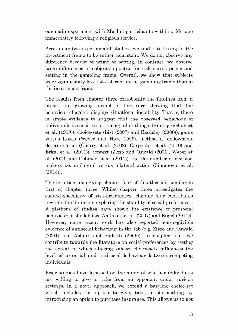
Across our two experimental studies, we find risk-taking in the

investment frame to be rather consistent. We do not observe any

difference because of prime or setting. In contrast, we observe

large differences in subjects’ appetite for risk across prime and

setting in the gambling frame. Overall, we show that subjects

were significantly less risk-tolerant in the gambling frame than in

the investment frame.

The results from chapter three corroborate the findings from a

broad and growing strand of literature showing that the

behaviour of agents displays situational instability. That is, there

is ample evidence to suggest that the observed behaviour of

individuals is sensitive to, among other things, framing (Schubert

et al. (1999)), choice-sets (List (2007) and Bardsley (2008)), gains

versus losses (Weber and Hsee 1999), method of endowment

determination (Cherry et al. (2002), Carpenter et al. (2010) and

Erkal et al. (2011)), context (Zizzo and Oswald (2001), Weber et

al. (2002) and Dohmen et al. (2011)) and the number of decision

makers i.e. unilateral versus bilateral action (Simunovic et al.

(2013)).

The intuition underlying chapter four of this thesis is similar to

that of chapter three. Whilst chapter three investigates the

context-specificity of risk-preferences, chapter four contributes

towards the literature exploring the stability of social-preferences.

A plethora of studies have shown the existence of prosocial

behaviour in the lab (see Andreoni et al. (2007) and Engel (2011)).

However, more recent work has also reported non-negligible

evidence of antisocial behaviour in the lab (e.g. Zizzo and Oswald

(2001) and Abbink and Sadrieh (2009)). In chapter four, we

contribute towards the literature on social-preferences by testing

the extent to which altering subject choice-sets influences the

level of prosocial and antisocial behaviour between competing

individuals.

Prior studies have focussed on the study of whether individuals

are willing to give or take from an opponent under various

settings. In a novel approach, we extend a baseline choice-set

which includes the option to give, take, or do nothing by

introducing an option to purchase insurance. This allows us to not

14

only test the extent to which individuals possess other-regarding

preferences, as in previous studies, but also whether subjects are

sufficiently concerned about the possibility of others taking money

from them and as a result willing to invest resources to avoid this.

Furthermore, we test if there is any difference in the observed

behaviour of subjects when any amount stolen from their

opponent is kept versus when it is simply burned (wasted).

Importantly, subjects are asked to make these decisions after

having competed for an endowment in a winner-takes-all

tournament setting.

Our results show that extending the available choice-set by

including the option to insure crowds out voluntary donations by

competition winners even when insurance represents a dominated

strategy in monetary terms. Moreover, switching the context of

the problem from potentially having one’s endowment stolen and

kept to having it burned by an opponent lowers prosociality in

terms of average donation size. In contrast, our data shows

considerable evidence of sabotage and antisocial behaviour by

contest losers that remains consistent across treatments. We

argue that the reduction in prosociality is driven by subjects’

unwillingness to steal from their poorer counterparts when there

is uncertainty regarding their chosen action whereas the

consistent taking by poor subjects is motivated by a strong

aversion towards disadvantageous inequality. The findings from

chapter four adds further support to the growing consensus on the

existence of other-regarding preferences as well as the situational

instability of preferences (List (2007), Bardsley (2008) and

Dohmen et al. (2011)).

Chapter five provides a brief summary and conclusion of our

research findings from chapters two, three and four.

15

CHAPTER TWO

2. Is Asset-Class Diversification

Beneficial for Shariah-Compliant Equity

Portfolios?

ABSTRACT

In this chapter, we study a) whether diversifying across asset-

classes by including commodities and Sukuk could improve the

performance of an equity-only Islamic portfolio b) the benefits of

diversification over historically significant bull and bear markets

to test the relevance of diversification during volatile and

trending markets c) the dynamic conditional correlation between

the aforementioned asset-classes to study how the relationship

across markets is affected during crisis regimes and d) we employ

a convenient tail-risk measure of performance which includes the

importance of an assets skewness and kurtosis to study whether

taking into account the shape of the returns distribution provides

further insight into the potential benefits of diversification. Our

findings suggest that the benefit of diversifying beyond an equity-

only portfolio is limited during normal times but much greater

during crisis periods, with improvement in both risk-return

profiles and the probability of extreme losses. Our most important

finding relates to the estimation of portfolio tail-risk. In

particular, we find that using a standard two-moment Value-at-

Risk measure, which assumes normally distributed returns,

rather than a four-moment Value-at-Risk, which incorporates an

assets skewness and kurtosis, can lead to a substantial


conditions. This result is especially important for Islamic portfolio

managers as Islamic securities are more likely to deviate from a

normal distribution for reasons such as market thinness, market

16

illiquidity, the lack of product standardization and the inability to

diversify across a broader range of markets.

2.1 INTRODUCTION

The Islamic finance sector has attracted considerable attention

recently due to its impressive performance and phase of

expansion since the subprime financial crisis. In particular, the

industry has experienced an annualized growth rate of

approximately 15% in global assets over the past decade, which

were in the region of $200 billion in 2003, $2.2 trillion in 2017 and

are forecasted to cross $3.8 trillion by 20221.

Shariah-compliant finance caters primarily for faith-based

economic agents whose religious motivation requires them to

operate under a dual-regulatory framework. That is, they must

incorporate both country-specific and religious-based legislation

within their decision-making framework, which seeks to

maximize both present and some notion of an afterlife utility.

Therefore, whilst the conceptual function of both conventional and

Islamic finance is identical i.e. facilitating agents in their desire to

smooth consumption patterns across time and space, Shariah-

compliance necessitates the imposition of additional constraints,

including a) the prohibition of interest b) the prohibition of

speculation and contractual ambiguity c) the exclusion of

financing and dealing with what the Islamic faith deems socially

irresponsible or unethical activities and d) a requirement that all

transactions be directly linked to the real underlying economic

transaction (Usmani (1998) and Gait and Worthington (2007)).

Islamic finance essentially imposes various screening criterion,

based on non-pecuniary value-judgements, to filter out what are

considered to be compliant investments out of the broader

universe of investable assets. In fact, such screening based on

subjective beliefs and value-judgements is what relates Shariah

compliant investing to the growing market for Socially-

Responsible Investments (SRI). Although there isn’t a

1 See Thomson Reuters (2017) and The City United Kingdom

Islamic Finance Report (2015)

17

unanimously agreed definition of what constitutes a socially-

responsible investment, EUROSIF (2014) defines SRI as any type

of investment process that combines investors’ financial objectives

with their concerns about environmental, social and governance

(ESG) issues. Hence, this leads to similarities between SRI and

Islamic finance as they both restrict or shrink the set of assets,

based on subjective values, in which their adherents may invest.

For example, both Islamic and SRI funds typically prohibit

investment into tobacco companies. That said, perhaps the key

difference between the two is that the filtering criterion may not

always be in alignment. This is exemplified by the fact that SRI

also involves, for example, screening investments based on

environmental issues, company governance structures and

engaging with companies that aim to improve social welfare. By

contrast, such strategies are typically not deemed necessary and

thus not implemented by Shariah compliant investors.

While there has been no empirical consensus in the literature,

several authors have argued that the additional constraints

imposed by Shariah compliance, which often alters the

characteristics and underlying structure of Islamic securities,

creates a theoretical heterogeneity between the conventional and

Islamic finance sectors that could result in differences in the

stability of either sector and their response to economic shocks

(Chapra (2008) and Hassan (2009))2. For example, Hassan and

Dridi (2010) describe how the Islamic banking sector initially

absorbed the financial crisis shock better than the conventional

sector due to factors attributed to their differing principles, such

as greater stringency on leverage ratios and the prohibition of

investing in so-called toxic derivative markets. However, Hassan

and Dridi (2010) also show that once the ramifications of the crisis

penetrated deeper into the real-economy, a combination of poor

risk-management and excessive sectoral concentration caused

substantial damage to the balance-sheets of Islamic financial

institutions.

The regulatory requirements put-forth by the Shariah create

several issues for Islamic portfolio managers. For instance, the

2 For studies finding no significant differences, see Cevik and

Charap (2011) and Chong and Lio (2009). For an alternative view,

see Rosly et al. (2003), Cakir and Raei (2007), Beck et al. (2013)

and Farooq and Zaheer (2015).

18

prohibition of ambiguity and uncertainty in contracts has

generally led Shariah boards and scholars to rule out any trade in

derivatives (Jobst and Sole 2012). Although the impermissibility

of investing in derivative contracts shielded Islamic portfolios

from subprime loans during the financial crisis, this constraint

may not be as beneficial in a wider context. That is, derivatives

help the economy achieve an efficient allocation of risk, assist in

completing markets, provide financial market participants with

information and may help reduce or hedge against risks (Sill

1997). This is further exacerbated by the prohibition of strategies

such as short-selling which violates the Islamic teaching that one

must not sell something that they do not possess or own (Usmani

1998). Therefore, from a theoretical perspective, Islamic portfolios

are more vulnerable to large fluctuations in value due to the

inability to use such financial instruments to hedge against

economic shocks (Hesse et al. 2008).

Secondly, the prohibition of investing in certain markets that are

deemed illegitimate e.g. alcohol, concentrates wealth across fewer

sectors, thus limiting the potential for diversification and

increasing the vulnerability of Shariah compliant portfolios to

extreme events and idiosyncratic shocks within particular

markets. Furthermore, given the relative infancy of the Islamic

finance sector, market participation is still relatively low and

there is an absence of mature secondary markets for important

securities such as Sukuk. This market thinness makes Shariah

compliant portfolios more susceptible to large fluctuations in

valuation. Moreover, there is a prevalence of buy-and-hold

investors within Sukuk markets. While this has been attributed

to an acute lack of supply, the shortage of liquidity this creates

not only hampers market growth but makes the valuation of

Sukuk more volatile during periods of crises (Hesse et al. (2008),

Sole (2008) and Kammer et al. (2015)).

A wider problem facing Islamic securities relates to the process of

their approval. That is, securities such as Sukuk must be

approved by a Shariah board prior to issuance. While the

existence of multiple boards creates issues pertaining to

standardization due to differences in the interpretation of Islamic

scripture (Ellis (2012) and Godlewski et al. (2014)), a further

concern brought to light in recent history is that these rulings

aren’t immune from being challenged post-issuance. More

19

precisely, a recent issuance of Islamic bonds was announced as

being non-compliant roughly three years after being on the

market and prior to the date of maturity. Although the legislative

basis for this declaration was contested, such issues within the

industry can greatly amplify risk and uncertainty (Ellis (2012)

and Jackson (2018)).

Recent evidence shows that Islamic portfolios are highly

concentrated within certain geographic regions, asset-classes and

market sectors. For example, in 2017, 87% of the Islamic asset-

management sector was concentrated within three countries i.e.

Iran, Malaysia and Saudi Arabia, where oil dependence is crucial

to growth (see Thomson Reuters 2018 report). Furthermore,

Islamic investors tend to have substantial equity holdings with

minimal diversification across asset-classes (see HSBC Amanah

(2011) and Mauro et al. (2013)). The aforementioned issues are

further exacerbated by the shrinking of the potential sectors

across which Islamic investors may diversify, which leads to

greater concentration in some specific sectors, such as Basic

Materials, Industrials, Oil, Gas and Technology, thus inducing

greater volatility in returns (Hussein and Omran (2005),

Dewandaru et al. (2015) and Charles et al. (2015)). For instance,

Charles et al. (2015) show that Shariah-screening reduces the

number of stocks included in the Islamic index by up to 60-70%.

Having access to the composition and sectoral breakdown of the

Islamic index, Charles et al. (2015) show that 73% of the Islamic

index is concentrated within the Technology, Health-Care,

Industrials, Oil, Gas and Basic Material sectors. In comparison,

they show that the corresponding figure for the conventional

index was only 49%.

In addition to the aforementioned challenges that compliant

portfolio managers face, a further and broader issue has been the

growing financial integration and interdependence between world

economies. That is, it is relatively well-established that greater

levels of financial liberalisation and globalisation have resulted in

tighter cross-border integration and interdependencies among

global equity markets (Kasa (1992), Corhay et al. (1993) and

Blackman and Thomas (1994)). A direct corollary of this

unprecedented increase in financial globalisation and the

subsequent increase in financial interdependence is that global

financial systems are now more vulnerable to systematic risk,

20

thus saturating the potential for cross-border diversification

opportunities within asset-classes. The increasing convergence of

risk-factors that global equity markets face has led several

authors to advocate for diversification across asset-classes.

Roll (2013) highlights the importance of diversifying across asset-

classes by arguing that even relatively well-diversified portfolios,

such as the S&P 500, are quite volatile during certain periods and

could benefit from extending their holdings across asset-classes to

diversify across risk-factors. Well-diversified portfolios within an

asset-class are highly-correlated, whereas well-diversified

portfolios across different asset-classes are less correlated. The

first point implies that there is a unique systematic factor that

limits diversification within an asset-class and the second implies

that each asset-class is mainly driven by its unique factor.

Studies such as Fugazza and Nicodano (2009), Arouri and Nguyen

(2010) and Daskalaki and Skiadopolous (2011) show that the

returns of securities within a particular asset-class display a

much higher correlation than they do with securities from

alternative asset-classes. Intuitively, this has to do with

heterogeneity in the underlying risk-factors across asset-classes.

This point is reinforced by Baur and Lucey (2010), Baur and

McDermott and Chan et al. (2011) who find that during periods of

higher risk-aversion i.e. economic downturns or crisis regimes,

investors attempt to preserve their wealth by shifting their

portfolios towards a greater allocation into so-called safe-haven

assets such as precious metals and treasuries, which tend to

display lower volatility and favourable hedging characteristics.

While the arguments in favour of multi asset-class portfolios have

gained considerable traction and support recently (Cheung and

Miu (2010), Su and Lau (2010), Hammoudeh et al. (2010), Arouri

et al. (2011) and Daskalaki and Skiadopolous (2011)), Chan et al.

(2011) argue that the benefits of diversification are highly regime-

specific. They find that during crisis regimes, the correlation

across asset-classes tends to increase, leaving little benefit from

diversification once transaction costs are accounted for.

In light of the regulatory restrictions the Shariah imposes on

Islamic securities and investors, in this chapter we study a)

whether diversifying across asset-classes by including

commodities and Sukuk could improve the performance of an

21

equity-only Islamic portfolio b) the benefits of diversification over

historically significant bull and bear markets to test the relevance

of diversification during volatile and trending markets c) the

dynamic conditional correlation between the aforementioned

asset-classes to study how the relationship across markets is

affected during crisis regimes and d) as explained earlier, given

that Islamic portfolios are more vulnerable to extreme events, we

employ a convenient tail-risk measure of performance which

includes the importance of an asset’s skewness and kurtosis to

study whether taking into account the shape of the returns’

distribution provides further insight into the potential benefits of

diversification.

An important objective of this study is to provide a comparative

analysis between the level of risk estimated when we use a

measure that assumes normally distributed returns versus a

measure that incorporates higher moments, such as an assets

skewness and kurtosis. Therefore, given the overall motivation of

our study, we use the Value-at-Risk (VaR) model for a few

important reasons. First, there is a lack of studies within the

Islamic finance literature that employ methods which are directly

understood and implementable by industry practitioners. The

VaR is beneficial in this regard since it is ubiquitous and thus

very well-known among practitioners. The Value-at-Risk was also

considered an attractive methodology for our analysis as it can be

used for non-normally distributed assets. The four-moment VaR,

covered in Section 2.3 (see Favre and Galeano 2002), adjusts the

Gaussian quantile function for skewness and kurtosis using the

Cornish-Fisher expansion (Cornish and Fisher 1937), thus

allowing us to provide a direct comparison between the level of

risk estimated by the standard two-moment and higher-moment

VaRs.

Hence, not only is the VaR straightforward in terms of

implementation, able to measure risk with just one easily

understandable number and able to incorporate higher-moments,

but this approach has a further added advantage of having been

embraced by European regulators (see EIOPA 2016). That is,

regulators such as the European Securities and Markets

Authority (ESMA) has adopted the Cornish-Fisher based VaR as

a standardised method to be used in order to report the embedded

risk of packaged retail investment and insurance based products

22

(PRIIPs), which generally include stocks, bonds, insurance

policies, structured funds, deposits and products.

However, although our approach does offer the advantages stated

above, an important limitation for the general purposes of

portfolio management is that the VaR is based upon a univariate

distribution. An alternative approach to modelling various risks

and the study of extremal events under a multivariate

distribution is that of copula analysis. The copula methodology,

first introduced by Sklar (1959), has received great attention in

the banking industry since it was first used for financial

applications by Embrechts et al. (1999). Therefore, although we

adopt the VaR for the reasons outlined above, an interesting

extension of our work, especially if there is a broader availability

of data on various Islamic assets, would be to use copula-analysis

to study portfolio management and extreme events within the

realm of Islamic finance.

2.2 PRIOR LITERATURE

The literature exploring the potential for diversification in

portfolios incorporating both Islamic and conventional equities

has increased substantially over the past decade. In particular,

much attention has been devoted towards studying the

relationship and co-movement between conventional and Islamic

equity markets. This is because researchers have primarily been

interested in testing whether Islamic stocks represent a unique

asset-class or whether they fall within the general class of

conventional equities (Hakim and Rashidian (2004), Hassan and

Girard (2010), Guyot (2011), Saiti and Masih (2014), Alexakis et

al. (2015), Ajmi et al. (2014) and Mensi et al. (2017)).

The empirical research on diversification both within and across

asset-classes that are specifically considered Shariah compliant

has been less forthcoming. Madjoub and Mansour (2014) study

the relationship between the Islamic equity indices of the U.S.

and a set of five emerging markets. The authors find evidence of

the U.S. market being only weakly correlated with the emerging

markets under consideration, which they attribute to the

principles of Islamic finance. Madjoub and Mansour (2014) argue

that the stringent restrictions on leverage ratios, interest-based

transactions and the asset-backed nature of Islamic investments

23

reduces the exposure of markets to volatility spillovers and thus

provides investors with diversification opportunities.

Similar to Madjoub and Mansour (2014), Abbess and Trichilli

(2015) investigate the potential benefits of diversifying Islamic

portfolios by combining stocks from developed and emerging

markets. Using a multivariate cointegration approach, Abbes and

Trichilli (2015) find that the degree of interdependence varies

depending on the level of economic similarity between the

markets under consideration. While markets within a particular

economic grouping i.e. developed or emerging display higher

levels of integration, there is some evidence that this relationship

is a lot weaker for those from opposing groups, suggesting that

there may be some scope for cross-border diversification in Islamic

equities.

Khan et al. (2015) investigate the time-varying correlation

dynamics between the Dow Jones Islamic equity index and

various commodity indices to determine the potential for

diversification between them. The authors find evidence of

instability in correlations which show a general tendency towards

increasing during periods of market stress, implying limited

diversification during bearish periods. However, Khan et al.

(2015) argue that the commodity sector cannot be considered a

homogenous asset-class, as the time-varying relationships vary

significantly depending on the type of commodity under

consideration. In a similar study, Abdullah, Saiti and Masih

(2016) find that the degree of interdependence between Islamic

equity and commodity markets is country-specific. Their findings

suggest that there may be scope for diversification based on

differences in risk-factors, which in some instances can have a

significant overlap between asset-classes within the realm of

Islamic finance. For example, oil prices are likely to be a lot more

correlated with equity prices in major oil-producing nations such

as Saudi Arabia than they are in those where oil production is

less significant, such as Pakistan.

Yilmaz et al. (2015) study the correlation dynamics between ten

Islamic equity sector indices i.e. stocks within the healthcare and

energy sectors, belonging to the family of Dow Jones Islamic

indices. Covering the period from 1999 to 2014, Yilmaz et al.

(2015) find an increase in the degree of sectoral integration and

interdependence over time, implying limited scope for

24

diversification within the equity asset-class. The authors argue

that a period of increasing global financialization has weakened

the importance of fundamentals and real economic factors in

determining equity prices which are now instead increasingly

driven by factors such as capital flows, risk-appetite, behavioural

factors and investment strategies.

Alaoui et al. (2015) explore the co-movement dynamics between

various regional equity indices within the Gulf Cooperation

Council and a global Sukuk index. They find strong evidence of

time-varying correlations, greater contagion between markets in

closer proximity and a flight-to-quality during the recent financial

crisis whereby investors sought to shift their portfolio weights

towards a greater allocation of Sukuk relative to equity holdings.

Nagayev et al. (2016) examine the extent to which commodity

markets co-move with Islamic equities. Their findings show that

the return correlations between equities and commodities are

time-varying and highly volatile, showing a substantial and

persistent increase in correlations during the global financial

crisis of 2008. Moreover, using a wavelet coherence model,

Nagayev et al. (2016) find that the benefit of investing in

commodities is dependent on an investor’s time-horizon. While

some commodities can provide short-term benefits, they may not

do so in the longer-run. However, once transaction costs are taken

into consideration, these short-term benefits may also be limited.

As described above, the existing literature on portfolio

diversification within the realm of Islamic finance primarily

focuses on econometric methods aimed at capturing correlations,

interdependencies and contagion effects between markets. Higher

statistical moments, such as skewness and kurtosis have

generally been ignored as a criterion for evaluating portfolio-

management decisions. However, it is well established in the

literature that financial returns typically display significant

skewness and kurtosis. Early researchers such as Rubinstein

(1973) argue that skewness and kurtosis cannot be ignored unless

asset returns are normally distributed and the investor’s utility

function is quadratic. If these two conditions were satisfied, the

first two moments would be sufficient for maximizing expected

utility. This is because a normal distribution implies that the

entire distribution of an assets returns could be inferred through

its mean and variance, making higher-moments irrelevant.

25

Likewise, if returns aren’t normally distributed but investors

have quadratic utility functions, then by construct, this would

assume that investors are indifferent to other features of the

distribution. However, quadratic utility assumes that investors

are equally averse to deviations above the mean as they are to

deviations below the mean, and that they sometimes prefer less

wealth to more wealth, which isn’t borne out by the data

(Cremers, Kritzman and Page 2004).

In a seminal paper, Harvey et al. (2010) propose a theoretical

model for optimal portfolio allocation that incorporates higher-

moments. The authors find that including higher-moments in the

decision process alters the optimal portfolio allocation and

increases expected utility. This general result has been reinforced

by a growing strand of empirical literature. You and Daigler

(2010) use a novel approach by exploring whether the inclusion of

higher-moments affects the purported benefits of diversifying

across international equity markets. Using a four-moment Value-

at-Risk methodology, the authors find that ignoring higher-order

moments, in particular an assets skewness and kurtosis, can lead

to an underestimation of the true level of portfolio risk.

Our main contribution towards the literature is to apply this four-

moment Value-at-Risk methodology to investigate whether

incorporating a more complete description of the shape of the

returns’ distribution of Shariah compliant financial securities

could provide Islamic portfolio managers with additional

information regarding a) the level of tail-risk contained within

their portfolios b) the extent to which diversifying across asset-

classes could potentially improve tail-risk and c) whether

neglecting higher moments affects the interpretation of portfolio

tail risk over bearish and bullish markets.

2.3. DATA AND METHODOLOGY

We obtain daily closing prices3 quoted in US dollars for the S&P

500 Shariah Index, Dow Jones Islamic Developed Market Equity

3 The issue of selecting an appropriate frequency for the data has

been a sensitive topic in the literature. While daily-data could

arguably better capture the fast-paced information transmission

26

Index, Dow Jones Islamic Emerging Market Equity Index, Dow

Jones Sukuk Index and the Goldman Sachs Commodity Spot

Indices for the Energy, Livestock, Agriculture, Industrial and

Precious Metal sectors. While investing in commodity futures isn’t

permissible under the principles of Shariah, spot trading, of

certain commodities, is deemed acceptable under several

standards (Usmani 1998). All data was sourced through the

Bloomberg Terminal. To perform our analysis, we generate daily

returns using the conventional formula:

𝑅𝑡 = (ln(𝑃𝑡) − ln(𝑃𝑡−1)) ∗ 100

(2.1)

Our dataset runs from the 8th of October 2007 to the 15th of March

2015 i.e. the beginning of the subprime financial crisis to the S&P

peak in March 2015, for a total of 1919 observations per series.

We split our data into two time periods to study the role of

diversification over a bear market period i.e. October 2007 to

March 2009 and the subsequent expansion or bull-period, albeit

with periodic market corrections, running from March 2009 to

March 2015. Our rationale for this is particularly to determine

the effects of the most extreme market conditions in recent times

i.e. the subprime financial crisis, which was the only major crisis

within the range of the available data.

The substantial evidence of time-varying correlation dynamics

between financial securities is especially relevant when assessing

the benefits of diversification (Longin and Solnik (1995), Tse

(2000) and Goetzmann et al. (2005)). This is because examining

how the behaviour and degree of interdependence between

securities changes during volatile periods or in response to

economic shocks provides information about the extent to which

and co-movements in financial-markets, as well as providing a

richer data-set in terms of observations, daily-data can also

involve greater statistical noise. In contrast, while using lower

frequency data could mitigate the problems associated with

excessive noise, it may result in biased estimations due to the

lower number of observations available. This issue is of great

relevance in the Islamic Finance sector as the poor-availability of

data exacerbates the trade-off between minimising noise and the

number of observations. More precisely, for our sample-interval,

using weekly-data would have provided approximately 360

observations whereas monthly-data would have only provided

approximately 120. For these reasons, we opted for daily-data.

27

their underlying risk-factors are aligned. Therefore, we employ

the Dynamic Conditional Correlation (DCC) model introduced by

Engle (2002). This model builds upon the framework of

ARCH/GARCH-type models developed by Engle (1982) and

Bollerslev (1986). Assuming that 𝑟𝑡 denotes a vector consisting of

two return series, 𝐴(𝐿) the lag polynomial and 𝜀𝑡 the error term

vector, then the return and conditional variance can be

represented as:

𝐴(𝐿)𝑟𝑡 = 𝜇 + 𝜀𝑡, 𝜀𝑡~𝑁(0,𝐻𝑡)

(2.2)

And,

𝐻𝑡 = 𝐷𝑡𝑅𝑡𝐷𝑡

(2.3)

Where𝐷𝑡 = 𝑑𝑖𝑎𝑔{√ℎ1,𝑡√ℎ2,𝑡} is the diagonal matrix of time-varying

standard deviations estimated from the univariate 𝐺𝐴𝑅𝐶𝐻(1,1)

models and 𝑅𝑡 is the time-varying conditional correlation matrix.

That is, in the first-stage of the DCC estimation, univariate

GARCH models are fit for both return series. In the second-stage,

the standardized residuals from the prior stage are used to obtain

the conditional correlation coefficients. The 𝐺𝐴𝑅𝐶𝐻(1,1) variance

is represented by:

ℎ𝑡 = 𝜔𝑖 + 𝛼𝑖𝜀𝑡−12 + 𝛽𝑖ℎ𝑡−1, 𝜔𝑖 , 𝛼𝑖,𝛽𝑖 > 0, 𝛼𝑖 + 𝛽𝑖 < 1

(2.4)

Where 𝜔𝑖 represents the weighted long-run variances whilst the 𝛼

and 𝛽 coefficients determine the short-term dynamics of the

volatility series resulting from the equation.

The time-varying correlation matrix, 𝑅𝑡, can be decomposed into:

𝑅𝑡 = 𝑄𝑡∗−1𝑄𝑡𝑄𝑡

∗−1

(2.5)

Where 𝑄𝑡 is the symmetric positive definite matrix of the

conditional variances-covariances and 𝑄𝑡∗−1 is an inverted

diagonal matrix consisting of the square root of the diagonal

elements of 𝑄𝑡 i.e.

𝑄𝑡∗−1 =

[

1

√𝑞11𝑡

0

01

√𝑞11𝑡]

(2.6)

28

And:

𝑄𝑡 = (1 − 𝜃1 − 𝜃2)�̅� + 𝜃1𝜀𝑡−1𝜀𝑡−1′ + 𝜃2𝑄𝑡−1

(2.7)

If both parameter estimates for 𝜃1, which measures the effect of

past shocks on current conditional correlation, and 𝜃2, which

measures the impact of past correlations, are significant, then

this would indicate that the conditional correlation between the

two series isn’t constant.

The dynamic conditional correlation between two assets, 1 and 2,

at time 𝑡 is given by:

𝜌12𝑡 =𝑞12𝑡

√𝑞11𝑡𝑞22𝑡

(2.8)

The coefficients in the DCC model are estimated by a two-step

maximum likelihood method, where the maximum likelihood

function is expressed as:

𝐿 =1

2∑ (2 log(2𝜋) + 2 log|𝐷𝑡| + log|𝑅𝑡| + 𝜀𝑡

′𝑅𝑡−1𝜀𝑡)

𝑇

𝑡=1

(2.9)

Deviations from constant correlations are not the only concern

when evaluating diversification benefits. Another common issue is

the potential deviation from a normal distribution. It is well

known that most financial returns data aren’t normally

distributed but rather often display non-zero skewness and

positive excess kurtosis values. Following the financial crisis,

market participants and academics have begun to question the

usefulness of standard deviation as a measure of risk. Many

financial-agents have begun the adoption of alternative models to

quantify portfolio risk, with the standard Value-at-Risk being

among the most common. This approach quantifies negative tail-

risk by identifying the expected potential loss with a hypothetical

fall in the market by a specified number of standard deviations

(Uludag and Ezzat 2016).

Coupled with the greater vulnerability of Shariah-compliant

assets to extreme events for reasons mentioned earlier, this

motivates the need to consider the role of higher statistical

moments when determining potential diversification benefits. We

29

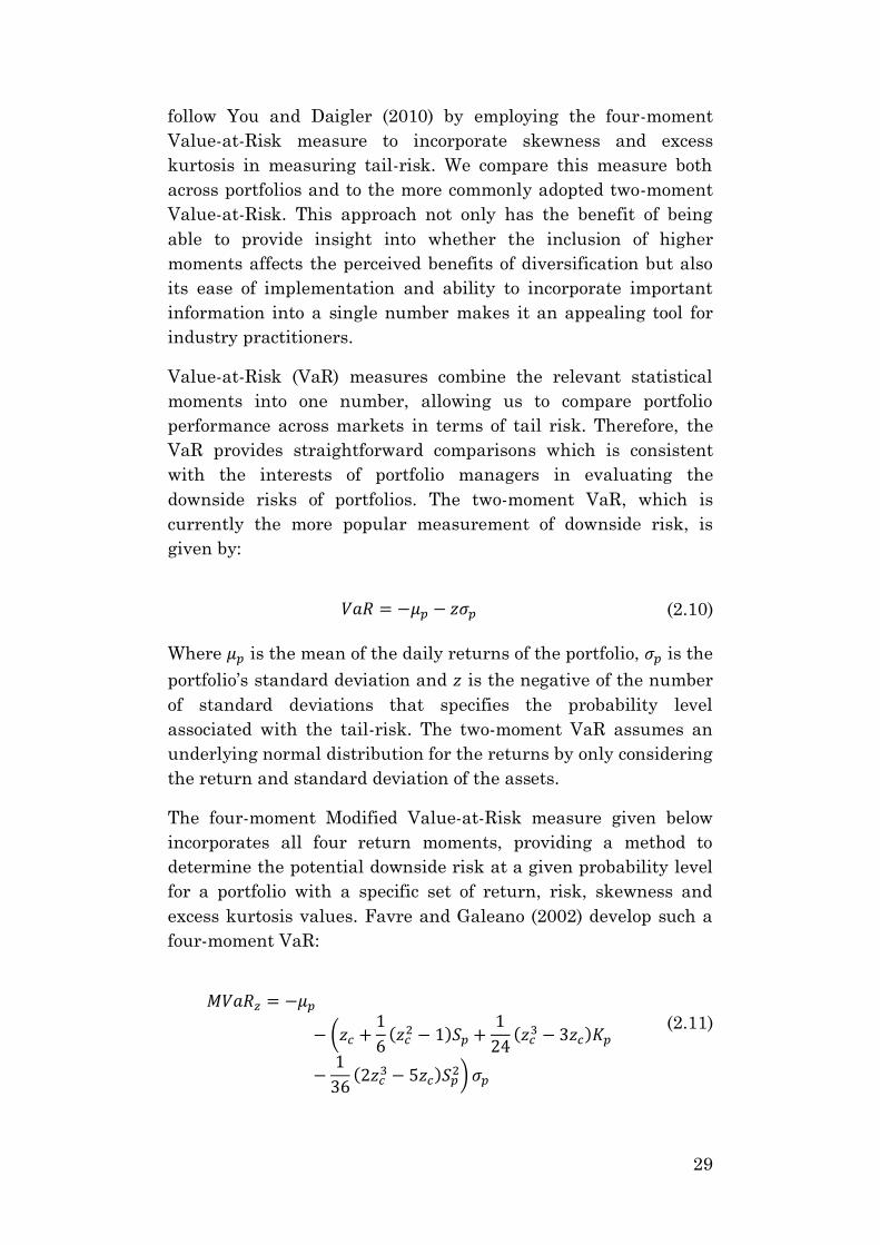
follow You and Daigler (2010) by employing the four-moment

Value-at-Risk measure to incorporate skewness and excess

kurtosis in measuring tail-risk. We compare this measure both

across portfolios and to the more commonly adopted two-moment

Value-at-Risk. This approach not only has the benefit of being

able to provide insight into whether the inclusion of higher

moments affects the perceived benefits of diversification but also

its ease of implementation and ability to incorporate important

information into a single number makes it an appealing tool for

industry practitioners.

Value-at-Risk (VaR) measures combine the relevant statistical

moments into one number, allowing us to compare portfolio

performance across markets in terms of tail risk. Therefore, the

VaR provides straightforward comparisons which is consistent

with the interests of portfolio managers in evaluating the

downside risks of portfolios. The two-moment VaR, which is

currently the more popular measurement of downside risk, is

given by:

𝑉𝑎𝑅 = −𝜇𝑝 − 𝑧𝜎𝑝

(2.10)

Where 𝜇𝑝 is the mean of the daily returns of the portfolio, 𝜎𝑝 is the

portfolio’s standard deviation and 𝑧 is the negative of the number

of standard deviations that specifies the probability level

associated with the tail-risk. The two-moment VaR assumes an

underlying normal distribution for the returns by only considering

the return and standard deviation of the assets.

The four-moment Modified Value-at-Risk measure given below

incorporates all four return moments, providing a method to

determine the potential downside risk at a given probability level

for a portfolio with a specific set of return, risk, skewness and

excess kurtosis values. Favre and Galeano (2002) develop such a

four-moment VaR:

𝑀𝑉𝑎𝑅𝑧 = −𝜇𝑝

− (𝑧𝑐 +1

6(𝑧𝑐

2 − 1)𝑆𝑝 +1

24(𝑧𝑐

3 − 3𝑧𝑐)𝐾𝑝

−1

36(2𝑧𝑐

3 − 5𝑧𝑐)𝑆𝑝2) 𝜎𝑝

(2.11)

30

Where 𝜇𝑝, 𝜎𝑝, 𝑆𝑝and 𝐾𝑝 are the first four moments of portfolio 𝑃,

and 𝑧𝑐 is the negative number of standard deviations that

specifies the tail probability level associated with the four-

moment VaR. the two-moment VaR is a special case of this four-

moment VaR when the skewness and excess kurtosis are zero.

2.4. EMPIRICAL RESULTS

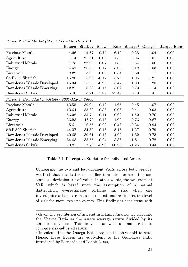
Table 2.1 reports the first four moments for each individual asset.

With the exception of the Precious Metals sector, each asset

displays a lower average return during period 1 (bear market)

than in period 2 (bull market) whereas every asset displays a

higher standard deviation during period 1. Most of the assets

under consideration display negative skewness and positive

excess kurtosis which, as evidenced by the Jarque-Bera tests

reported in the final column of Table 2.1, implies that returns do

not follow a normal distribution and thus motivates the need to

include higher moments when assessing the potential benefits of

portfolio diversification.

On average, Islamic equity markets outperform commodities and

Sukuk in terms of risk-adjusted returns during the bull market.

This finding is reversed during the bear market where

commodities and Sukuk outperform equities. Shariah compliant

equities, on average, display greater positive kurtosis than

commodities while Sukuk have the largest kurtosis values. This

reinforces our earlier argument regarding the relatively greater

vulnerability of Islamic securities to extreme events. The thinner

tails and superior performance of commodities during the bear

market could make them valuable to compliant portfolio

managers for purposes of risk-mitigation.

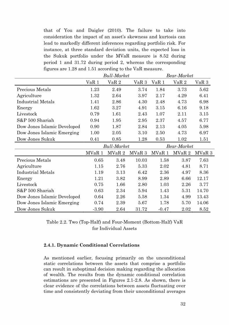
Tables 2.2 reports the two and four-moment VaRs at one, two and

three standard deviations for each of the assets individually.

Intuitively, a higher standard deviation implies that we are

further into the left-hand tail of the distribution and thus

progressively considering higher volatility or more extreme

scenarios (Uludag and Ezzat 2016).

31

Period 2: Bull Market (March 2009-March 2015)

Return Std.Dev Skew Kurt Sharpe4 Omega5 Jarque-Bera

Precious Metals 4.66 19.87 -0.75 6.19 0.23 1.04 0.00

Agriculture 1.14 21.01 0.08 1.53 0.05 1.01 0.00

Industrial Metals 7.73 22.92 -0.07 1.83 0.34 1.06 0.00

Energy 4.57 26.06 -0.17 3.05 0.18 1.03 0.00

Livestock 8.22 13.05 -0.03 0.54 0.63 1.11 0.00

S&P 500 Shariah 16.88 15.98 -0.17 3.70 1.06 1.21 0.00

Dow Jones Islamic Developed 15.34 15.33 -0.26 3.42 1.00 1.20 0.00

Dow Jones Islamic Emerging 12.21 16.66 -0.15 3.02 0.73 1.14 0.00

Dow Jones Sukuk 5.40 6.91 5.87 153.47 0.78 1.41 0.00

Period 1: Bear Market (October 2007-March 2009)

Precious Metals 13.55 30.04 0.12 1.65 0.45 1.07 0.00

Agriculture -13.64 33.62 -0.38 0.98 -0.41 0.93 0.00

Industrial Metals -56.92 35.74 -0.11 0.63 -1.59 0.76 0.00

Energy -36.23 47.79 -0.16 1.09 -0.76 0.87 0.00

Livestock -5.61 16.55 -0.23 0.46 -0.34 0.94 0.00

S&P 500 Shariah -44.37 34.89 0.18 5.18 -1.27 0.79 0.00

Dow Jones Islamic Developed -49.65 30.61 -0.16 4.90 -1.62 0.73 0.00

Dow Jones Islamic Emerging -64.43 35.55 -0.24 3.88 -1.81 0.72 0.00

Dow Jones Sukuk -9.81 7.79 -5.99 60.20 -1.26 0.44 0.00

Table 2.1. Descriptive Statistics for Individual Assets

Comparing the two and four-moment VaRs across both periods,

we find that the latter is smaller than the former at a one

standard deviation cut-off value. In other words, the two-moment

VaR, which is based upon the assumption of a normal

distribution, overestimates portfolio tail risk when one

investigates a less extreme scenario and underestimates the level

of risk for more extreme events. This finding is consistent with

4 Given the prohibition of interest in Islamic finance, we calculate

the Sharpe Ratio as the assets average return divided by its

standard deviation. This provides us with a simple ratio to

compare risk-adjusted return. 5 In calculating the Omega Ratio, we set the threshold to zero.

Hence, these figures are equivalent to the Gain-Loss Ratio

introduced by Bernardo and Ledoit (2000)

32

that of You and Daigler (2010). The failure to take into

consideration the impact of an asset’s skewness and kurtosis can

lead to markedly different inferences regarding portfolio risk. For

instance, at three standard deviation units, the expected loss in

the Sukuk portfolio under the MVaR measure is 8.52 during

period 1 and 31.72 during period 2, whereas the corresponding

figures are 1.28 and 1.51 according to the VaR measure.

Bull-Market Bear-Market

VaR 1 VaR 2 VaR 3 VaR 1 VaR 2 VaR 3

Precious Metals 1.23 2.49 3.74 1.84 3.73 5.62

Agriculture 1.32 2.64 3.97 2.17 4.29 6.41

Industrial Metals 1.41 2.86 4.30 2.48 4.73 6.98

Energy 1.62 3.27 4.91 3.15 6.16 9.18

Livestock 0.79 1.61 2.43 1.07 2.11 3.15

S&P 500 Shariah 0.94 1.95 2.95 2.37 4.57 6.77

Dow Jones Islamic Developed 0.90 1.87 2.84 2.13 4.05 5.98

Dow Jones Islamic Emerging 1.00 2.05 3.10 2.50 4.73 6.97

Dow Jones Sukuk 0.41 0.85 1.28 0.53 1.02 1.51


MVaR 1 MVaR 2 MVaR 3 MVaR 1 MVaR 2 MVaR 3

Precious Metals 0.65 3.48 10.03 1.58 3.87 7.63

Agriculture 1.15 2.76 5.33 2.02 4.81 8.71


Energy 1.21 3.82 8.99 2.89 6.66 12.17

Livestock 0.75 1.66 2.80 1.03 2.26 3.77

S&P 500 Shariah 0.63 2.34 5.94 1.43 5.31 14.70

Dow Jones Islamic Developed 0.64 2.26 5.58 1.34 4.99 13.43

Dow Jones Islamic Emerging 0.74 2.39 5.67 1.78 5.70 14.06

Dow Jones Sukuk -3.90 2.64 31.72 -0.47 2.02 8.52

Table 2.2. Two (Top-Half) and Four-Moment (Bottom-Half) VaR

for Individual Assets

2.4.1. Dynamic Conditional Correlations

As mentioned earlier, focusing primarily on the unconditional

static correlations between the assets that comprise a portfolio

can result in suboptimal decision making regarding the allocation

of wealth. The results from the dynamic conditional correlation

estimations are presented in Figures 2.1-2.8. As shown, there is

clear evidence of the correlations between assets fluctuating over

time and consistently deviating from their unconditional averages

33

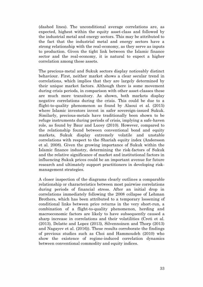
(dashed lines). The unconditional average correlations are, as

expected, highest within the equity asset-class and followed by

the industrial metal and energy sectors. This may be attributed to

the fact that the industrial metal and energy sectors have a

strong relationship with the real-economy, as they serve as inputs

to production. Given the tight link between the Islamic finance

sector and the real-economy, it is natural to expect a higher

correlation among these assets.

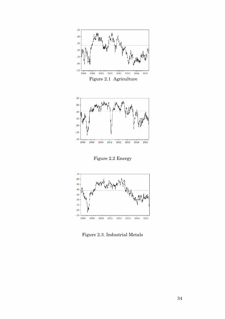
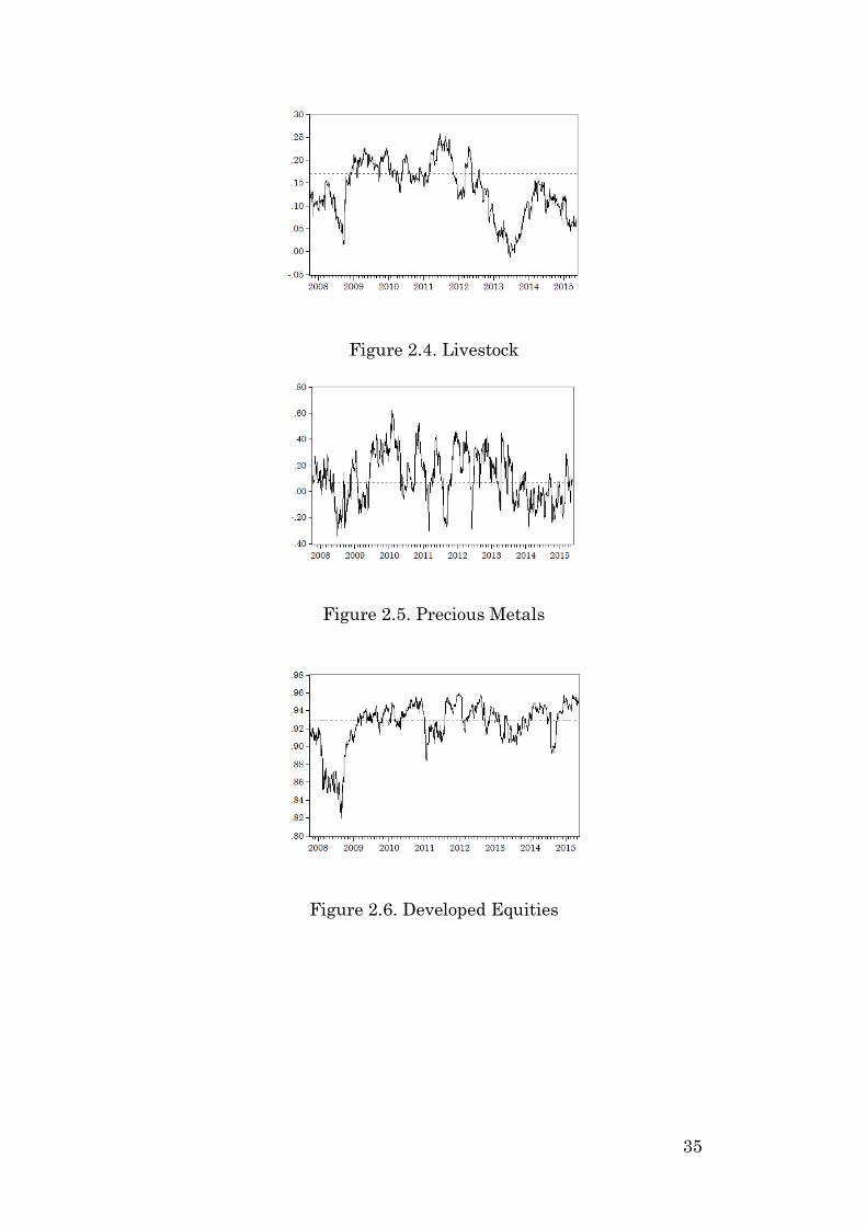
The precious-metal and Sukuk sectors display noticeably distinct

behaviour. First, neither market shows a clear secular trend in

correlations, which implies that they are largely determined by

their unique market factors. Although there is some movement

during crisis periods, in comparison with other asset-classes these

are much more transitory. As shown, both markets display

negative correlations during the crisis. This could be due to a

flight-to-quality phenomenon as found by Alaoui et al. (2015)

where Islamic investors invest in safer sovereign-issued Sukuk.

Similarly, precious-metals have traditionally been shown to be

refuge instruments during periods of crisis, implying a safe-haven

role, as found by Baur and Lucey (2010). However, compared to

the relationship found between conventional bond and equity

markets, Sukuk display extremely volatile and unstable

correlations with respect to the Shariah equity index (Andersson

et al. 2008). Given the growing importance of Sukuk within the

Islamic finance industry, determining the risk-factors of Sukuk

and the relative significance of market and institutional factors in

influencing Sukuk prices could be an important avenue for future

research and ultimately support practitioners in developing risk-

management strategies.

A closer inspection of the diagrams clearly outlines a comparable

relationship or characteristics between most pairwise correlations

during periods of financial stress. After an initial drop in

correlations immediately following the 2008 collapse of Lehman

Brothers, which has been attributed to a temporary loosening of

conditional links between price returns in the very short-run, a

combination of a flight-to-quality phenomenon, herding and

macroeconomic factors are likely to have subsequently caused a

sharp increase in correlations and their volatilities (Creti et al.

(2013), Delatte and Lopez (2013), Silvennoinen and Thorp (2013)

and Nagayev et al. (2016)). These results corroborate the findings

of previous studies such as Choi and Hammoudeh (2010) who

show the existence of regime-induced correlation dynamics

between conventional commodity and equity indices.

34

Figure 2.1 Agriculture

Figure 2.2 Energy

Figure 2.3. Industrial Metals

35

Figure 2.4. Livestock

Figure 2.5. Precious Metals

Figure 2.6. Developed Equities

36

Figure 2.7. Emerging Market Equities

Figure 2.8. Sukuk

Figures 2.1-2.8: Dynamic Conditional Correlations between S&P

500 Shariah and Stated Assets (Dashed Line Represents Static

Correlations)

Following the crisis we generally find a persistent correlation

dynamic, with correlations remaining high until a dip in 2012.

This has been attributed to a combination of macroeconomic,

political, financial and behavioural factors over the 2008-2012

period (Nagayev et al. 2016). The systemic nature of the crisis

caused widespread panic and negative market sentiment at a

global scale that affected most markets in similar ways (Bain

2014). The increased dependence and spill-over between asset-

markets was likely due to liquidity constraints faced by investors

as sources of borrowing dried up, which forced investors to sell

assets at fire-sale prices in order to restore balance-sheets

(Delatte and Lopez 2013). In turn, this led to asset prices

generally moving in the same direction, which again highlights

37

the fact that Islamic equities aren’t insulated from general

market conditions.

More generally, a sharp increase in the popularity of commodity

investing over the past decade has triggered an unprecedented

inflow of institutional funds into commodity futures markets

(Basak and Pavlova 2015). This phenomenon has been referred to

as the financialization of commodities. From a theoretical

perspective, the fundamental valuation of an asset is determined

by its expected discounted cash flows. However, since the

financialization of commodities, it has been argued that factors

other than the primary supply and demand of commodities, such

as the speculation phenomenon often seen in energy markets,

which are also susceptible to behavioural biases, now have a

significant influence on commodity prices. A direct corollary of the

increased financialization has been argued to be greater volatility

in commodity markets and correlations between commodity and

equity markets (Tang and Xiong 2012). Given the relationship

between futures and spot prices, activity in the futures market

has a direct feedback into spot markets (Girardi 2012). Coupled

with the tight-link between the Islamic sector and the real-

economy, which is affected by commodity prices, these factors

imply that Islamic portfolios with commodity holdings are not

insulated from activity in the conventional sector, as reflected by

the fact that the correlation dynamics closely resemble those

found between conventional equity and commodity markets6.

These findings raise additional concerns regarding immunization

strategies for Islamic portfolio managers as it further limits their

potential to hedge and diversify risk.

However, correlations between Islamic equity and commodity

returns have shown a decline since 2012. Various explanations

have been put-forth regarding this apparent reversal in

correlations. Terazono (2015) argues that according to the

physical supply and demand view, commodity markets are now

normalizing and will likely return to an era where they are more

influenced by individual supply and demand fundamentals. Bain

(2014) suggests that commodity valuations have been impacted by

uncertainty regarding the economic growth trajectory of countries

such as China. Based on the financialization view, the reduction

of activity in commodity markets has led to the decrease in

6 See, for example, Creti et al. (2013).

38

correlations. A combination of tighter regulation, growing capital

requirements and the peaking possibility of the commodity super-

cycle has led to large financial institutions lowering their

exposure to commodity markets (Sheppard (2014) and Kaminska

(2014)).

2.4.2. Portfolio Diversification7

Following You and Daigler (2010), You and Nguyen (2013) and

Daigler et al. (2017), we compose the desired portfolios by

adopting a straightforward risk-return framework in order to

identify the Markowitz mean-variance optimal allocations.

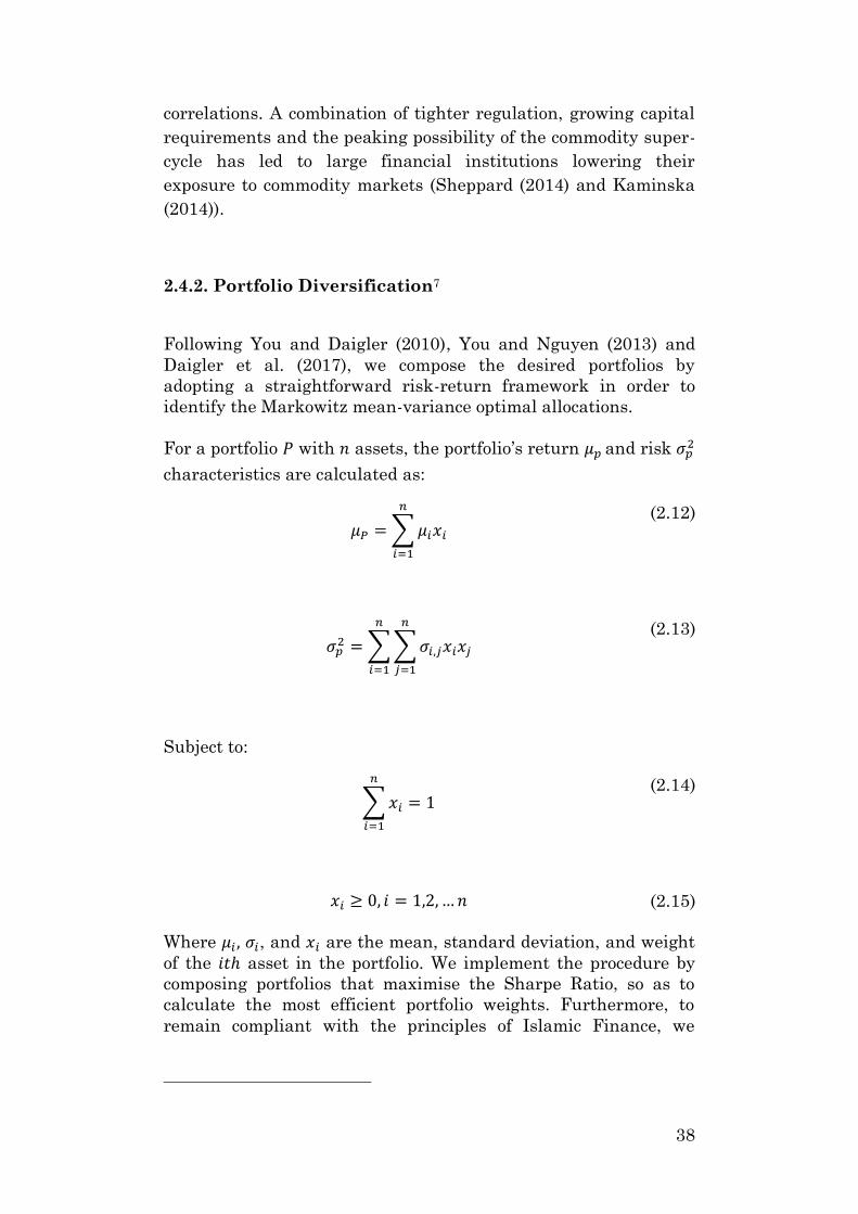
For a portfolio 𝑃 with 𝑛 assets, the portfolio’s return 𝜇𝑝and risk 𝜎𝑝2

characteristics are calculated as:

𝜇𝑃 = ∑ 𝜇𝑖𝑥𝑖

𝑛

𝑖=1

(2.12)

𝜎𝑝2 = ∑∑𝜎𝑖,𝑗𝑥𝑖𝑥𝑗

𝑛

𝑗=1

𝑛

𝑖=1

(2.13)

Subject to:

∑𝑥𝑖 = 1

𝑛

𝑖=1

(2.14)

𝑥𝑖 ≥ 0, 𝑖 = 1,2,… 𝑛

(2.15)

Where 𝜇𝑖 , 𝜎𝑖, and 𝑥𝑖 are the mean, standard deviation, and weight

of the 𝑖𝑡ℎ asset in the portfolio. We implement the procedure by

composing portfolios that maximise the Sharpe Ratio, so as to

calculate the most efficient portfolio weights. Furthermore, to

remain compliant with the principles of Islamic Finance, we

39

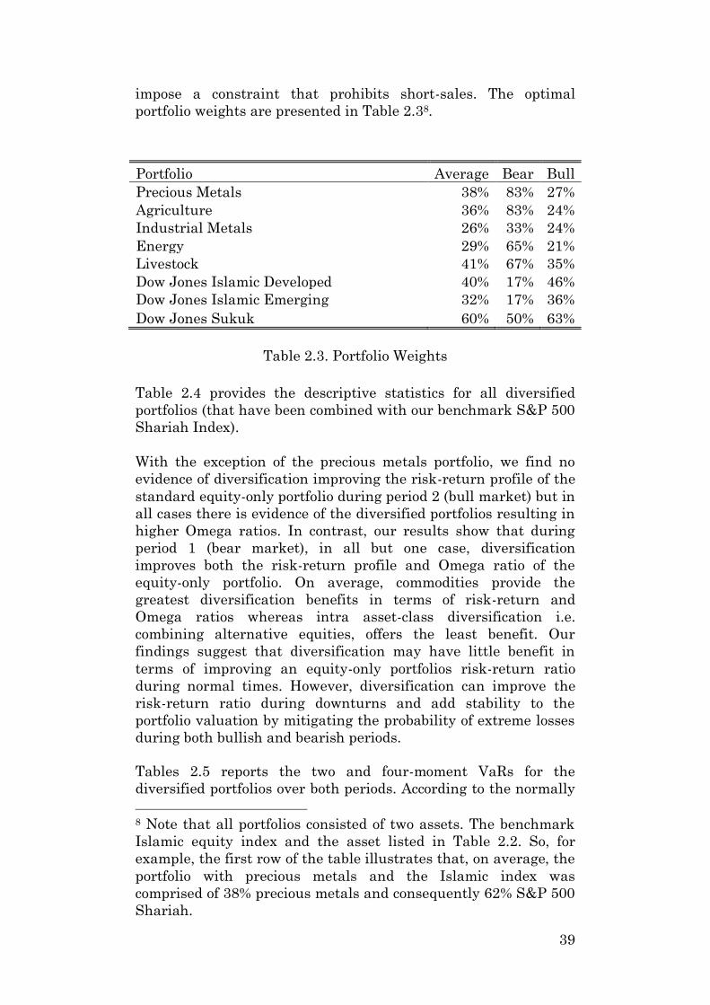
impose a constraint that prohibits short-sales. The optimal

portfolio weights are presented in Table 2.38.

Portfolio Average Bear Bull

Precious Metals 38% 83% 27%

Agriculture 36% 83% 24%

Industrial Metals 26% 33% 24%

Energy 29% 65% 21%

Livestock 41% 67% 35%

Dow Jones Islamic Developed 40% 17% 46%

Dow Jones Islamic Emerging 32% 17% 36%

Dow Jones Sukuk 60% 50% 63%

Table 2.3. Portfolio Weights

Table 2.4 provides the descriptive statistics for all diversified

portfolios (that have been combined with our benchmark S&P 500

Shariah Index).

With the exception of the precious metals portfolio, we find no

evidence of diversification improving the risk-return profile of the

standard equity-only portfolio during period 2 (bull market) but in

all cases there is evidence of the diversified portfolios resulting in

higher Omega ratios. In contrast, our results show that during

period 1 (bear market), in all but one case, diversification

improves both the risk-return profile and Omega ratio of the

equity-only portfolio. On average, commodities provide the

greatest diversification benefits in terms of risk-return and

Omega ratios whereas intra asset-class diversification i.e.

combining alternative equities, offers the least benefit. Our

findings suggest that diversification may have little benefit in

terms of improving an equity-only portfolios risk-return ratio

during normal times. However, diversification can improve the

risk-return ratio during downturns and add stability to the

portfolio valuation by mitigating the probability of extreme losses

during both bullish and bearish periods.

Tables 2.5 reports the two and four-moment VaRs for the

diversified portfolios over both periods. According to the normally

8 Note that all portfolios consisted of two assets. The benchmark

Islamic equity index and the asset listed in Table 2.2. So, for

example, the first row of the table illustrates that, on average, the

portfolio with precious metals and the Islamic index was

comprised of 38% precious metals and consequently 62% S&P 500

Shariah.

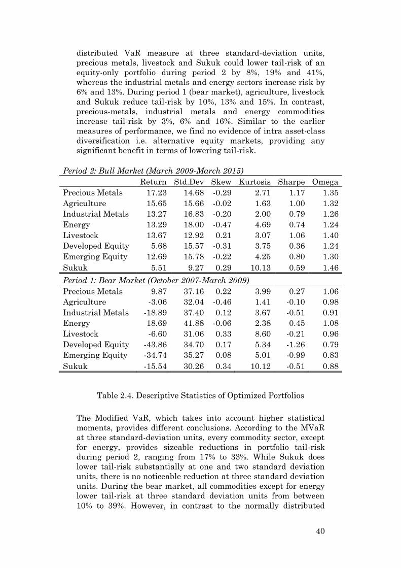
40

distributed VaR measure at three standard-deviation units,

precious metals, livestock and Sukuk could lower tail-risk of an

equity-only portfolio during period 2 by 8%, 19% and 41%,

whereas the industrial metals and energy sectors increase risk by

6% and 13%. During period 1 (bear market), agriculture, livestock

and Sukuk reduce tail-risk by 10%, 13% and 15%. In contrast,

precious-metals, industrial metals and energy commodities

increase tail-risk by 3%, 6% and 16%. Similar to the earlier

measures of performance, we find no evidence of intra asset-class

diversification i.e. alternative equity markets, providing any

significant benefit in terms of lowering tail-risk.

Period 2: Bull Market (March 2009-March 2015)

Return Std.Dev Skew Kurtosis Sharpe Omega

Precious Metals 17.23 14.68 -0.29 2.71 1.17 1.35

Agriculture 15.65 15.66 -0.02 1.63 1.00 1.32

Industrial Metals 13.27 16.83 -0.20 2.00 0.79 1.26

Energy 13.29 18.00 -0.47 4.69 0.74 1.24

Livestock 13.67 12.92 0.21 3.07 1.06 1.40

Developed Equity 5.68 15.57 -0.31 3.75 0.36 1.24

Emerging Equity 12.69 15.78 -0.22 4.25 0.80 1.30

Sukuk 5.51 9.27 0.29 10.13 0.59 1.46

Period 1: Bear Market (October 2007-March 2009)

Precious Metals 9.87 37.16 0.22 3.99 0.27 1.06

Agriculture -3.06 32.04 -0.46 1.41 -0.10 0.98

Industrial Metals -18.89 37.40 0.12 3.67 -0.51 0.91

Energy 18.69 41.88 -0.06 2.38 0.45 1.08

Livestock -6.60 31.06 0.33 8.60 -0.21 0.96

Developed Equity -43.86 34.70 0.17 5.34 -1.26 0.79

Emerging Equity -34.74 35.27 0.08 5.01 -0.99 0.83

Sukuk -15.54 30.26 0.34 10.12 -0.51 0.88

Table 2.4. Descriptive Statistics of Optimized Portfolios

The Modified VaR, which takes into account higher statistical

moments, provides different conclusions. According to the MVaR

at three standard-deviation units, every commodity sector, except

for energy, provides sizeable reductions in portfolio tail-risk

during period 2, ranging from 17% to 33%. While Sukuk does

lower tail-risk substantially at one and two standard deviation

units, there is no noticeable reduction at three standard deviation

units. During the bear market, all commodities except for energy

lower tail-risk at three standard deviation units from between

10% to 39%. However, in contrast to the normally distributed

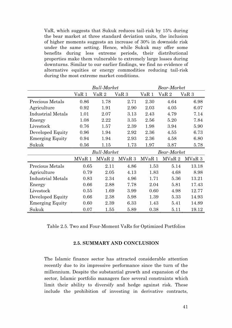
41

VaR, which suggests that Sukuk reduces tail-risk by 15% during

the bear market at three standard deviation units, the inclusion

of higher moments suggests an increase of 30% in downside risk

under the same setting. Hence, while Sukuk may offer some

benefits during less extreme periods, their distributional

properties make them vulnerable to extremely large losses during

downturns. Similar to our earlier findings, we find no evidence of

alternative equities or energy commodities reducing tail-risk

during the most extreme market conditions.


VaR 1 VaR 2 VaR 3 VaR 1 VaR 2 VaR 3

Precious Metals 0.86 1.78 2.71 2.30 4.64 6.98

Agriculture 0.92 1.91 2.90 2.03 4.05 6.07


Energy 1.08 2.22 3.35 2.56 5.20 7.84

Livestock 0.76 1.57 2.39 1.98 3.94 5.90

Developed Equity 0.96 1.94 2.92 2.36 4.55 6.73

Emerging Equity 0.94 1.94 2.93 2.36 4.58 6.80

Sukuk 0.56 1.15 1.73 1.97 3.87 5.78


MVaR 1 MVaR 2 MVaR 3 MVaR 1 MVaR 2 MVaR 3

Precious Metals 0.65 2.11 4.86 1.53 5.14 13.18

Agriculture 0.79 2.05 4.13 1.83 4.68 8.98


Energy 0.66 2.88 7.78 2.04 5.81 17.43

Livestock 0.55 1.69 3.99 0.60 4.98 12.77

Developed Equity 0.66 2.38 5.98 1.39 5.33 14.93

Emerging Equity 0.60 2.39 6.33 1.43 5.41 14.89

Sukuk 0.07 1.55 5.89 0.38 5.11 19.12

Table 2.5. Two and Four-Moment VaRs for Optimized Portfolios

2.5. SUMMARY AND CONCLUSION

The Islamic finance sector has attracted considerable attention

recently due to its impressive performance since the turn of the

millennium. Despite the substantial growth and expansion of the

sector, Islamic portfolio managers face several constraints which

limit their ability to diversify and hedge against risk. These

include the prohibition of investing in derivative contracts,

42

engaging in short-selling, investing in markets considered

illegitimate by the Shariah and the insufficient liquidity and lack

of standardization in Islamic bond markets. This is further

exacerbated by the more general finding that the process of

financial globalisation has resulted in increasing integration,

interdependence and contagion between international equity

markets.

In light of these issues, in this chapter we studied a) whether

diversifying across asset-classes by including particular compliant

commodities and Sukuk could improve the performance of equity-

only Islamic portfolios b) the benefits of diversification over



dynamic nature of correlations between the aforementioned asset-

classes and d) given that Islamic portfolios are more vulnerable to

extreme events, we employed a convenient tail-risk measure of

performance which includes the importance of an assets skewness

and kurtosis to study whether taking into account the shape of

the returns distribution provides further insight into the potential

benefits of diversification.

Our findings show that the benefit of diversifying beyond an

equity-only portfolio is minimal during normal times in terms of

improvement in risk-return profiles but there is some evidence

that diversification can lower the chances of extreme losses

during such periods. In contrast, we find that the benefits of

diversification are much greater during crisis periods, with

improvement in both risk return profiles and Omega ratios.

However, our most important finding relates to the estimation of

portfolio tail-risk. In particular, we find that using a standard

two-moment Value-at-Risk measure, which assumes normally

distributed returns, rather than a four-moment Value-at-Risk,

which incorporates an assets skewness and kurtosis, can lead to a

substantial underestimation of portfolio risk during the most

extreme market conditions. This result is especially important for

Islamic portfolio managers as Islamic securities are more likely to

deviate from a normal distribution for reasons such as market

thinness, market illiquidity, the lack of product standardization

and the inability to diversify across a broader range of markets.

While these findings could motivate several strands of future

research, such as extending our analysis to cover additional

43

markets and securities as well as studying the risk-factors of

Islamic securities, the challenges facing the Islamic finance

industry, such as the lack of market liquidity, insufficient hedging

instruments, inadequate secondary markets and the lack of

product standardization perhaps require the greatest attention.

44

2.6. REFERENCES

1. Abbes, M.B. and Trichilli, Y. (2015). Islamic stock markets

and potential diversification benefits. Borsa Istanbul

Review, 15(2), 93-105.

2. Abdullah, A.M, Saiti, B. and Masih, M. (2016). The impact

of crude oil on Islamic stock indices of South-East Asian

countries: Evidence from MGARCH-DCC and wavelet

approaches. Borsa Istanbul Review, 16(4), 219-232.

3. Ajmi, A.N., Hammoudeh, S., Nguyen, D.K, Sarfrazi, S.

(2014). How strong are the causal relationships between

Islamic stock markets and conventional financial systems?

Evidence from linear and non-linear tests. Journal of

International Financial Markets, Institutions and Money,

28, 213-227.

4. Alaoui, E., Abdelkader, O., Dewandaru, G., Rosly, S. and

Masih, M. (2015). Linkages and co-movement between

international stock market returns: Case of Dow Jones

Islamic Dubai financial market index, Journal of


36, 53-70.

5. Alexakis, C., Pappas, V. and Tsikouras, A. (2015). Long-run

asymmetric relationships between Islamic and

conventional equity indices, Lancaster University School of

Economics Working Paper.

6. Andersson, M., Krylova, E. and Vahamaa, S. (2008). Why

does the correlation between stock and bond returns vary

over time? Applied Financial Economics, 18(2), 139-151.

7. Arouri, M. and Nguyen, D. (2010). Oil prices, stock markets

and portfolio investment: Evidence from sector analysis in

Europe over the last decade. Energy Policy, 38(8), 4528-

4539.

8. Arouri, M., Jouini, J. and Nguyen, D.K. (2011). Volatility

spillovers between oil prices and stock sector returns:

Implications for portfolio management. Journal of

International Money and Finance, 30(7), 1387-1405.

9. Bain, C. (2014). What next for commodity price

correlations? (Article), Capital Economics, London, United

Kingdom.

10. Basak, S. and Pavlova, A. (2015). A model of

financialization of commodities. CEPR Discussion Paper.

45

11. Baur, D.G. and Lucey, B.M. (2010). Is gold a hedge or safe

haven? An analysis of stocks, bonds and gold. Financial

Review, 45, 217-229.

12. Baur, D.G. and McDermott, T.K. (2010), Is gold a safe

haven? International evidence. Journal of Banking and

Finance, 34(8), 1886-1898.

13. Beck, T., Kunt, A. and Merrouche, O. (2013). Islamic vs

conventional banking: Business model, efficiency and

stability. Journal of Banking and Finance, 37(2), 433-447.

14. Bernardo, A.E. and Ledoit, O. (2000). Gain, loss and asset

pricing. Journal of Political Economy, 108, 144-172.

15. Blackman, S., Holden, K. and Thomas, W. (1994). Long-

term relationships between international share prices.

Applied Financial Economics, 4(4), 297-304.

16. Bollerslev, T. (1986). Generalized autoregressive

conditional heteroskedasticity. Journal of Econometrics, 31,

307-327.

17. Cakir, S. and Raei, F. (2007). Sukuk vs Eurobond: Is there

a difference in value-at-risk? IMF Working Paper.

18. Cevik, S. and Charap, J. (2011). The behaviour of

conventional and Islamic bank deposit returns in Malaysia

and Turkey. IMF Working Paper.

19. Chan, K.F., Treepongkaruna, S., Brooks, R. and Gray, S.

(2011). Asset market linkages: Evidence from financial,

commodity and real-estate assets. Journal of Banking and

Finance, 35(6), 1415-1426.

20. Chapra, U. (2008). The global financial crisis: Can Islamic

finance help minimize the severity and frequency of such a

crisis in the future? Presentation at the forum on the global

financial crisis at the Islamic Development Bank.

21. Charles, A., Darne, O. and Pop, A. (2015). Risk and ethical

investment: empirical evidence from Dow Jones Islamic

indexes. Research in International Business and Finance,

35, 33-56.

22. Cheung, C.S. and Miu, P. (2010). Diversification benefits of

commodity futures. Journal of International Financial

Markets, Institutions and Money, 20(5), 451-474.

23. Choi, K. and Hammoudeh, S. (2010). Volatility behaviour of

oil, industrial commodity and stock markets in a regime-

switching environment. Energy Policy, 38(8), 4388-4399.

46

24. Chong, B. and Liu, M. (2009). Islamic banking: Interest free

or interest based? Pacific-Basin Finance Journal, 17, 125-

144.

25. Corhay, A., Tourani Rad, A. and Urbain, J.P. (1993).

Common stochastic trends in European stock markets.

Economics Letters, 42(4), 385-390.

26. Cremers, J., Kritzman, M. and Page, S. (2004). Optimal

hedge fund allocations: Do higher moments matter? Revere

Street Working Paper.

27. Creti, A., Joets, M. and Mignon, V. (2013). On the links

between stock and commodity markets’ volatility. Energy

Economics, 37, 16-28.

28. Daigler, R., Dupoyet, B. and You, L. (2017). Spicing up a

portfolio with commodity futures: still a good recipe?

Journal of Alternative Investments, 19(4), 8-23.

29. Daskalaki, C. and Skiadopoulos, G. (2011). Should

investors include commodities in their portfolio after all?

New evidence. Journal of Banking and Finance, 35(10),

2606-2626.

30. Delatte, A. and Lopez, C. (2013). Commodity and equity

markets: Some stylized facts from a copula approach.

Journal of Banking and Finance, 37(12), 5346-5356.

31. Dewandaru, G., Bacha, O.I., Masih, A.M. and Masih, R.

(2015). Risk-return characteristics of Islamic equity indices:

multi-timescales analysis. Journal of Multinational

Financial Management, 29, 115-138.

32. EIOPA. (2016). European insurance and occupational

pensions authority. Final draft regulatory technical

standards.

33. Ellis, T. (2012). The piety premium of Islamic bonds.

Middle East Quarterly (Spring), 61-72.

34. Embrechts, P., Resnick, S. and Samorodnitsky, G. (1999).

Extreme value theory as a risk management tool. North

American Actuarial Journal, 3(2), 30-41.

35. Engle, R.F. (1982). Autoregressive conditional

heteroscedasticity with estimates of the variance of United

Kingdom inflation. Econometrica, 50(4), 987-1007.

36. Engle, R.F. (2002). Dynamic conditional correlation: A

simple class of multivariate GARCH. Journal of Business

and Economics Statistics, 20(3), 339-350.

47

37. EUROSIF. (2014). European sustainable investment forum

research division, socially responsible investment (SRI)

study.

38. Farooq, M. and Zaheer, S. (2015). Are Islamic banks more

resilient during financial panics? IMF Working Paper.

39. Favre, L. and Galeano, L.A. (2002). Mean-modified value-

at-risk optimization with hedge funds. Journal of

Alternative Investments, 5, 2-21.

40. Fugazza, C. and Nicodano, G. (2009). Time and risk

diversification in real-estate investments: Assessing the ex-

post economic value. Real Estate Economics, 37(3), 341-

381.

41. Gait, A.H. and Worthington, A.C. (2007). A primer on

Islamic finance: Definitions, sources, principles and

methods. University of Wollongong, School of Accounting

and Finance Working Paper.

42. Girardi, D. (2012). Do financial investors affect the price of

wheat? PSL Quarterly Review, 65(260), 79-109.

43. Godlewski, C.J., Turk, R. and Weill, L. (2014). Do the type

of Sukuk and choice of Shariah scholar matter? IMF

Working Paper.

44. Goetzmann, W.N., Li, L. and Rouwenhorst, K.G. (2005).

Long-term global market correlations. Journal of Business,

78, 1-38.

45. Guyot, A. (2011). Efficiency and dynamics of Islamic

investment: Evidence of geopolitical effects on Dow Jones

Islamic market indexes. Emerging Markets Finance and

Trade, 47(6), 24-45.

46. Hakim, S. and Rashidian, M. (2004). Risk and return of

Islamic stock indices. Paper presented at the International

Seminar of Non-Bank Financial Institutions: Islamic

Alternatives, Kuala Lumpur, Malaysia, March 1-3.

47. Hammoudeh, S., Yuan, Y., McAleer, M. and Thompson, M.

(2010). Precious metals – exchange rate volatility

transmissions and hedging strategies. International Review

of Economics and Finance, 19(4), 633-647.

48. Harvey, C.R., Liechty, J.C., Liechty, M.W. and Muller, P.

(2010). Portfolio selection with higher moments.

Quantitative Finance, 10(5), 469-485.

49. Hassan, A. (2009). The global financial crisis and Islamic

banking. (Article). Islamic Economics Unit, The Islamic

Foundation, United Kingdom.

48

50. Hassan, K. and Girard, E. (2010). Faith-based ethical

investing: The case of Dow Jones Islamic indexes. Islamic

Economic Studies, The Islamic Research and Training

Institute, 17, 1-31.

51. Hassan, K. and Kayed, R. (2009). The global financial

crisis, risk-management and social justice in Islamic

finance. ISRA International Journal of Islamic Finance, 1,

33-58.

52. Hassan, M. and Dridi, J. (2010). The effects of the global

crisis on Islamic and conventional banks: A comparative

study, IMF Working Paper.

53. Hesse, H., Jobst, A. and Sole, J. (2008). Trends and

challenges in Islamic finance. World Economics, 9(2), 175-

193.

54. HSBC Global Asset Management (2011), Introduction to

Islamic investing (Article), HSBC Amanah, London.

55. Hussein, K. and Omran, M. (2005). Ethical investment

revisited: evidence from Dow Jones Islamic indexes.

Journal of Investing, 14(3), 105-124.

56. ICD Thomson Reuters (2017), Islamic Finance

Development Report (2017).

57. Jackson, O. (2018). Primer: Islamic finance and Sukuk

explained. (Article). International Financial Law Review,

London, United Kingdom.

58. Kaminska, I. (2014). On the intriguing drop in commodity

correlation. (Article). Financial Times, London, United

Kingdom.

59. Kammer, A., Norat, M., Pinon, M., Prasad, A., Towe, C. and

Zeidane, Z. (2015). Islamic finance: Opportunities,

challenges and policy options, IMF Staff Discussion Note.

60. Kasa, K. (1992). Common stochastic trends in international

stock markets. Journal of Monetary Economics, 29, 95-124.

61. Khan, A.P., Kabir, S.K., Bashar, O. and Masih, M. (2015).

Time-varying correlation between Islamic equity and

commodity returns: Implications for portfolio

diversification. Journal of Developing Areas, 49(5), 115-128.

62. Longin, F. and Solnik, B. (1995). Is the correlation in

international equity returns constant: 1970-1990? Journal

of International Money and Finance, 14, 3-26.

63. Madjoub, J. and Mansour, W. (2014). Islamic equity market

integration and volatility spillover between emerging and

49

US stock markets. North American Journal of Economics

and Finance, 29, 452-470.

64. Markowitz, H. (1952). Portfolio selection. The Journal of

Finance, 7, 77-97.

65. Mauro, F., Caristi, P., Couderc, S., Di-Maria, A., Ho, L.,

Grewal, B.K., Masciantonio, S., Ongena, S. and Zaher, S.

(2013). Islamic finance in Europe. European Central Bank

Occasional Paper Series.

66. Mensi, W., Hammoudeh, S., Sensoy, A. and Yoon, S.M.

(2017). Analysing dynamic linkages and hedging strategies

between Islamic and conventional sector equity indexes.

Applied Economics, 49(25), 2456-2479.

67. Nagayev, R., Disli, M., Inghelbrecht, K. and Ng, A. (2016).

On the dynamic links between commodities and Islamic

equity. Energy Economics, 58, 125-140.

68. Roll, R. (2013). Volatility, correlation and diversification in

a multi-factor world. Journal of Portfolio Management,

39(2), 11-18.

69. Rosly, S.A. and Abu Bakar, M.D. (2003). Performance of

Islamic and mainstream banks in Malaysia. International

Journal of Social Economics, 30(12), 1249-1265.

70. Rubinstein, M. (1973). The fundamental theorem of

parameter-preference security valuation. Journal of

Financial and Quantitative Analysis, 8, 61-69.

71. Saiti, B. and Masih, M. (2014). The co-movement of

selective conventional and Islamic stock markets in East

Asia: Is there any impact on Shariah compliant equity

investment in China. University of Kuala Lumpur

(Malaysia) Working Paper.

72. Sheppard, D. (2014). Influence of banks, hedge-funds on

commodities lowest since 2008. (Article). Reuters, London,

United Kingdom.

73. Sill, K. (1997). The economic benefits and risks of

derivative securities. Business Review, Federal Reserve

Bank of Philadelphia.

74. Silvennoinen, A. and Thorp, S. (2013). Financialization,

crisis and commodity correlation dynamics. Journal of


24, 42-65.

75. Sklar, A. (1959). Fonctions de répartition à n dimensions et

leurs marges. Publications de l’Institut de Statistique de

l’Université de Paris, 8, 229–231.

50

76. Sole, J. (2008). Prospects and challenges for developing

corporate Sukuk and bond markets, lessons from a Kuwait

case study. International Journal of Islamic and Middle

Eastern Finance and Management, 1, 20-30.

77. Sole, J. and Jobst, A. (2012). Operative principles of Islamic

derivatives – towards a coherent theory. IMF Working

Paper.

78. Su, Y. and Lau, C.K.M. (2010). Strategic asset allocation

and intertemporal hedging demands with commodities as

an asset class. Suffolk University Working Paper.

79. Tang, K. and Xiong, W. (2012). Index investing and the

financialization of commodities. Financial Analysts

Journal, 68(6), 54-74.

80. Terazono, E. (2015). Commodity prices go back to basics.

(Article). Financial Times, London, United Kingdom.

81. The City UK Islamic Finance Report (2015), The City UK

Islamic Finance Market Advisory Group, London, United

Kingdom.

82. Thomson Reuters. (2018). Islamic finance development

report.

83. Tse, Y.K. (2000). A test for constant correlations in

multivariate GARCH model. Journal of Econometrics, 98,

107-127.

84. Uludag, B.K. and Ezzat, H. (2016). Are frontier markets

worth the risk? In P. Andrikopoilos, G.N. Gregoriou and V.

Kallinterakis (ed.), Handbook of Frontier Markets:

Evidence from Asia and International Comparative

Studies, Elsevier Inc., 67-80.

85. Usmani, T. (1998). An introduction to Islamic finance. (1st

ed.), Idaratul Ma`arif, Karachi, Pakistan.

86. Yilmaz, M.K., Sensoy, A., Ozturk, K. and Hachihasanoglu,

E. (2015). Cross-sectoral interactions in Islamic equity

markets. Pacific-Basin Finance Journal, 32, 1-20.

87. You, L. and Daigler, R.T. (2010). Is international

diversification really beneficial? Journal of Banking and

Finance, 34, 163-173.

88. You, L. and Nguyen, D. (2013). Higher order moment risk

in efficient futures portfolios. Journal of Economics and

Business, 65, 33-54.

51

CHAPTER THREE

3. Does Religious Priming and Decision-

Task Framing Influence Individual Risk-

Preferences?

ABSTRACT

We report the results of two experiments in which we explore the

extent to which elicited risk attitudes are influenced by framing

and religious priming. We find that risk-taking is significantly

higher when an identical task is framed in terms of investment

rather than gambling. We also find that a religious prime or

setting (a Mosque) significantly lowers risk-taking in the

gambling frame. One implication of our results is that risk

elicitation methods should avoid a gambling frame. In the

gambling frame we find that elicited risk-aversion is influenced by

a range of factors, including gender, ethical standards and the

setting, while in the investment frame we observe no such effects.

52

3.1. INTRODUCTION

Risk-aversion constitutes one of the most fundamental properties

of human behaviour. The seminal and pioneering work of

Bernoulli9 on gambling and the St. Petersburg Paradox in the 17th

century instigated substantial academic discourse and research

devoted towards developing a greater understanding of the

human decision-making process in situations involving risk. A

significant focus of this research has been on measuring risk-

aversion at the individual level and exploring factors, such as

gender, that may influence the extent of risk-aversion (Weber et

al. 2002).

Estimates and measures of risk-aversion have been studied and

developed in various settings (see Harrison and Röstrom (2008)

and Holt and Laury (2014) for a review). These include lab

experiments and surveys (Gneezy and Potters (1997), Eckel and

Grossman (2002), Lejuez et al. (2002), Holt and Laury (2002),

Weber, Blais and Betz (2002), Charness and Gneezy (2010) and

Dohmen et al. (2011)), labor-supply behaviour (Chetty 2006),

portfolio choices among financial investors (Mehra and Prescott

(1985) and Guiso and Paiella (2008)), option prices (Ait-Sahalia

and Lo 2000), deductive choices in insurance contracts (Szpiro

(1986) and Cohen and Einav (2007)), auction behaviour (Lu and

Perrigne 2008) and even contestant behaviour on game shows

(Post, Van Den Assem, Baltussen and Thaler (2008) and

Andersen, Harrison, Lau and Rustrom (2008)).

While the catalogue of studies providing methods of estimating

risk-preferences is clearly voluminous, considerable research has

documented evidence that measured risk-attitudes often vary

within individuals across elicitation techniques (See Johnson and

Rojas 2007). Importantly, it is not the case of there being a scaling

effect in that a particular method simply makes everyone seem

more or less risk-averse by a given proportion. Rather, there

seems to be a significant reordering of individuals in terms of the

ranking of their implied risk-parameters (Isaac and James 2000).

These results are consistent with the findings from a vast

literature within psychology showing that risk-preferences are

domain-specific (MacCrimmon and Wehrung (1986) and Weber et

9 See Bernoulli (1954)

53

al. (2002)). More precisely, individual risk-preferences do not

display cross-situational stability, which implies that even if the

objective numerical risk-return profiles are identical across two

domains, individuals may actually prefer or be less-willing to take

risks in one of those domains.

A leading explanation for why we may observe differences in risk-

taking across domains has been the individual’s perception and

trade-off between an activity’s benefits and risk. That is,

analogous to risk-return models in finance, such as the Capital

Asset Pricing Model, researchers have argued that risk-attitude

may be more usefully conceptualized in a psychological risk-

return framework. Psychological risk-return models treat

perceived riskiness as a variable that can differ between

individuals and as a function of content and context (Deck et al.

2010). This provides for multiple ways in which characteristics of

the decision maker and/or situation can affect choices under risk.

Apparent risk-taking by the same decision-maker may differ if

they perceive the risks and benefits to differ in magnitude across

the two domains e.g. in a recreational versus a financial decision,

while their attitude towards perceived risk essentially remains

identical across both domains.

Therefore, if an individual is faced with two opportunities that

offer identical objective risk-return profiles but they consider one

activity as either being less beneficial or riskier to engage in,

perhaps for some wider subjective reasons, then we may observe

differences in behaviour across those two domains. In other

words, it is conceivable that there exist deeper considerations,

such as the content-specificity of the action, which individuals

take into account during their decision-making process, rather

than purely basing their actions on quoted monetary values.

The existing evidence relating to the significance of the content

and domain specificity of risk-preferences could have important

ramifications for research eliciting measures of risk aversion. This

is because much of the experimental research eliciting risk-

preferences has the decision-task framed or presented in terms of

lotteries and gambling. For example, in the well-known Gneezy

and Potters (1997) experiment, participants are asked to decide

the portion of their endowment they “wish to bet in the following

lottery”, Eckel and Grossman (2002) measure risk attitudes by

presenting participants with six possible “gambles” and asking

54

them to choose the one they would most prefer to play. Similarly,

Benjamin et al. (2010) study how social identity affects risk-

preferences by presenting participants with 18 binary choices

between a safe option and a gamble, with their instructions

stating that “gambles would be resolved by drawing from a bag of

red and blue marbles.”

Frames like the three examples above suggest a gambling

connotation which could be influencing results. Intuition behind

this claim stems from the observation that gambling ostensibly

seems to be stigmatized across multiple cultures. While there

have been various explanations for why this may be, one possible

explanation is that the world’s major religions don’t look upon

gambling favourably (Binde 2007). Although there are varying

degrees of ambiguity in the condemnation of gambling across

religions10, the consensus among most sects across religious

ideologies considers gambling as being morally objectionable11.

Therefore, this argument postulates that due to the historically

influential role religion has had on the human race, the aversion

towards gambling may possibly have been ingrained into us over

the centuries.

If there is indeed a negative aura surrounding gambling, then

using lottery-type tasks to elicit risk-preferences could be

inadvertently priming subjects in a way that leads to an

underestimation of overall risk-preferences, with this effect being

more pronounced for particular demographics, such as the

religious. Moreover, using results from abstract gambling tasks as

proxies for risk attitudes to be applied in any context may lead to

misleading inferences. In other words, previous studies that have

been based on gambling frames have used their results to argue

that religious agents display higher levels of risk-aversion than

the irreligious. In this chapter, we argue that the religious may

appear more risk-averse in these studies since the task is framed

as a gamble (religious subjects are more likely to dislike

10 For instance, in Hinduism, Karma plays a central role and so

the precise motives behind why exactly it is that someone is

gambling will often have to be taken into consideration before

determining whether or not such actions are deemed acceptable. 11 Christianity: Exodus 20:17, Timothy 6:10. Luke 12:15, Matthew

6:24 and Hebrews 13:15, Judaism: Talmud (Sanhedrin: 24),

Islam: Quran (5:90), Hinduism: Rigveda Mandala 10, Sukta 34,

Buddhism: Sigalovada Sutta.

55

gambling). Hence, if one interprets the results from such studies

as religious people displaying greater levels of risk-aversion in

general, then this wouldn’t be correct as gambling frames may be

biasing the results.

In this study, we contribute towards the literature in three ways.

First, we test the proposition that the way in which the decision-

task is framed can influence risk-taking behaviour. We do this by

maintaining an identical numerical problem and manipulating

the framing of the decision-task to see whether this influences the

risk-appetite of participants in an incentivised lab experiment.

The two frames we use are an investment frame and a gambling

frame. Across two experiments, we observe significantly less risky

behaviour in gambling than in investing. This is consistent with

the notion that a gambling frame overestimates risk aversion.

Second, alongside employing a framing manipulation, we also test

whether priming subjects to make religion, or perhaps more

accurately some broader notion of ethics and morality, salient

influences behaviour. The purpose of priming one’s religious

identity is that it can temporarily increase the strength of one’s

affiliation with that identity category, causing their behaviour to

shift towards the category’s norms (Benjamin et al. 2016). Our

motivation in using the priming task was to see if the investment

versus gambling framing effect is more pronounced when subjects

are given a religious prime. This would be evidence that ethics

and morality are factors behind an aversion to gambling. Our

results point to an interesting dynamic effect in which those given

the religious prime react differently to a loss. This ultimately

means that those given a religious prime gamble less.

Finally, in a novel setup, we conduct a framing experiment within

a religious setting. More precisely, we ran an experiment with

Muslim participants, within the Mosque, immediately following a

religious service. The purpose of doing so was to test whether

greater religious intensity leads to a more pronounced difference

in risk-taking across the gambling and investment frames. The

framing effect we observed was extreme with hardly any risk

taking in the gambling frame. This finding reinforces results from

across our experimental studies that the framing effect varies

predictably with situation and individual characteristics.

56

Across our two experimental studies risk taking in the investment

frame was remarkably constant. We did not observe any

difference because of prime (religious or neutral) or setting

(Mosque, computer lab or classroom). Moreover, there was no

gender difference. By contrast, in the gambling frame we observe

big variations across prime, setting and gender. We would

suggest, therefore, that studies looking to elicit an individual’s

general attitude to risk should not use a frame that alludes to

gambling. Instead more neutral frames should be employed.

Whilst evidence of a significant framing effect has clear

implications in terms of experimental research on risk-

preferences, such religious or ethical framing may also have real-

world applications. In general, the relevance of framing can be

deduced by how ubiquitous the emphasis and advertisement of

the ethical and moral aspects of businesses has become. For

instance, firms commonly utilise marketing campaigns to promote

and differentiate themselves from competitors through

emphasising fair-trade policies, ethically-raised and free-from

produce, employee pay and working conditions, environmental

sustainability, charitable activities, gender equality and various

other ethical or moral features of their business. The importance

of framing or promoting such aspects of a business is clearly

importance since a recent report found that 92% of millennials are

more likely to purchase from what they consider an ethical

company and 66% are likely to invest in a company well-known

for its corporate social responsibility program (Aflac 2015).

In addition, to provide an example that perhaps more directly

relates to our research, consider a simple loan contract. Lenders

provide borrowers with funding in exchange for an overall

repayment that exceeds the amount initially lent. This excess

demanded over the original amount borrowed typically contains

compensation for the level of risk assumed by the lender and is

commonly referred to as an interest rate. However, under Islamic

law, interest is strictly prohibited. Modern Islamic banking

circumvents this issue by essentially rephrasing or repackaging

such compensation as a “profit-rate”. In other words, assuming

two identical loan contracts, simply manipulating or reframing

the compensation for risk as profit rather than interest can alter

whether certain agents consider the contract permissible or not.

Although there is little research in this area, evidence of a

57

significant framing effect in our experiment suggests that it may

be of interest to test how altering the framing of interest rates for

mortgage contracts or student-loans influences participation and

enrolment by Islamic agents in such productive investments.

3.2. PRIOR LITERATURE

There are two strands of literature related to our study. The first

strand compares risk-preferences between different faith-groups

and between religious and non-religious. The second looks at

framing effects on risky behaviour.

A general finding from studies comparing risk-preferences across

faith groups is that the religious appear (weakly) more risk-averse

than the irreligious (e.g. Bartke and Schwarz 2008, Hilary and

Hui 2009, Noussair et al. 2012). This result has sometimes been

explained through the fact that irreligious individuals essentially

take the riskier option in Pascal’s wager12 and are thus in general

more likely to display a greater appetite for risk than religious

individuals. The basic theme of our study, however, is that

measurement of risk aversion may interact with religiosity. It is

important, therefore, to consider how risk aversion is measured

and whether this may bias results.

An interesting comparison is that between Barsky et al. (1997)

and Halek and Eisenhaur (2001). Measuring risk aversion using

hypothetical questions about whether the person would take a job

that could improve or worsen family income, Barsky et al. (1997)

find evidence that Protestants are more risk averse than

Catholics who are more risk averse than Jewish.13 By contrast,

Halek and Eisenhaur (2001) using life-insurance data, find that

12 See Miller and Hoffman (1995) 13 It’s interesting to note that the sample used by Barsky et al.

(1997) was restricted to adults aged between 51 and 61. Some

authors have argued that religion becomes more salient during

older ages as individuals approach the later stages of their

lifecycle and could thus be more inclined to play the safer option

in Pascal’s wager. In this case using lottery-based tasks seems

undesirable since the conflict between gambling and religion

could be influencing the behaviour of participants and thus not

providing a true reflection of risk-aversion in other domains.

58

Catholics are marginally more risk averse than Protestants.14

They also, though, are able to measure risk aversion using the

same hypothetical questions as Barsky et al. (1997). Here they

find, consistent with Barsky et al. (1997) that Protestants are

more risk averse than Catholics.

Halek and Eisenhaur (2001) put this ‘flipping’ of risk attitudes

down to different preferences for speculative risk. For instance,

they point out that Protestants are more likely to view gambling

as sinful (see also Kumar et al. (2011) and Benjamin et al. (2016)).

If so, this would illustrate that attitudes to risk are sensitive to

context. There is the additional concern that choices made in

hypothetical situations may not reflect actual behaviours when

real money is at stake. Furthermore, evidence from experimental

economics suggests that respondent’s reports of their own

attitudes don’t always reflect their actual behaviours (e.g.

Glaesers et al. 2000). In emotive contexts such as religion,

questionnaire responses may be particularly subject to

conformity, self-image or desirability biases.

A further illustration of the way risk preferences can be

influenced by the interaction between religion and context is

provided by Leon and Pfeifer (2013). They use a German survey

data to investigate whether religiosity explains a household’s

willingness to take financial risks. Compared to the irreligious,

Christians were more willing to take financial risks through

holding larger positions in equities whereas Muslims were less

risk-taking with relatively larger investments in real-estate

compared to equities. However, Leon and Pfeifer (2013) also find

that Muslims are less likely to invest in life insurance compared

to the irreligious whereas Christians were more likely to do so.

Given that these results seem contradictory, as we would expect

risk-averse individuals to be more likely to purchase life-

insurance, one potential explanation of these findings could be

that the Islamic faiths prohibition on certain types of investment

are driving the decisions to abstain from equity and insurance

market investments.

Another study related to our work is that of Benjamin et al.

(2016). In their study, an unscrambling exercise was used to make

14 The sample size for Jewish is small but in terms of the raw

coefficient they display more risk aversion than Catholics.

59

religion salient for some participants. The sentences varied

depending on whether the subject was part of the religion-salient

condition or the control group.15 Benjamin et al. (2016) then use a

multiple price type lottery experiment to elicit risk attitudes. The

authors find that religious identity salience causes both Catholics

and the irreligious to become less risk-averse, but has no

significant effect for Protestants and Jews. The authors argue

that the strength of the identity salience manipulation could vary

by religious group, making them more likely to find null effects in

some groups than in others. Even so, it is a surprise to see less

risk-aversion with the religious prime. We obtain different results

as we shall discuss more below.

We will highlight one further study on risk aversion and religion

as it is one of the studies that has data on Muslims. Bartke and

Schwarz (2008) use self-reported survey data to examine the

relationship between religion and risk-aversion among German

immigrants. Muslim migrants were found to be more risk-averse

than their Christian counterparts, which was attributed to the

degree of strictness or comprehensiveness of the behavioural rules

embedded within a particular religion.

The preceding discussion has highlighted how risk preferences

may depend on an interaction between religion and context or

framing. The more general notion that elicited risk preferences

depend on context and framing of choice is well known. Indeed,

research has shown that there is little situational stability in

preferences (Deck et al. 2010). That is, there is little consistency

in people’s risk-taking attitudes across decision domains,

including gains versus losses (Weber and Hsee 1999), money

versus time domains (Weber and Milliman 1997), and gambling,

financial investing, business decisions and personal decisions

(MacCrimmon and Wehrung 1986, 1990).

Schubert et al. (1999) provide a particularly interesting example

of how the context and framing of a question can influence

15 Five of the ten sentences unscrambled by religion-salient

subjects contained religious content. The possible unscrambled

sentences for this group were as follows 1) she felt the spirit 2) the

desert was divine 3) her presence was appreciated 4) do it once

more 5) I mailed it over 6) give thanks to God 7) he finished it

yesterday 8) the book was sacred 9) prophets reveal the future

and 10) I was somewhat prepared.

60

findings and the subsequent policy prescriptions derived from

them. Several studies have found evidence of strong gender-

effects whereby women display significantly greater levels of risk-

aversion than their male counterparts (e.g. Croson and Gneezy

(2009) and Booth and Nolen (2012)). However, Schubert et al.

(1999) argue that such studies are strongly dependent on the

framing of the decision task. That is, while gender specific risk

propensities do arise in abstract gambling tasks, with males

showing a greater appetite for risky behaviour, the authors argue

that such differences in risk-attitudes are eliminated when the

decision task is reframed as an investment decision. Hence, they

suggest that abstract gambling experiments may be inadequate

for the analysis of gender-specific risk attitudes towards financial

decisions as in practice risky financial decisions are inherently

contextual (Schubert et al. 1999). Our results will reinforce this

conclusion.

In an influential paper, Weber et al. (2002) introduce the so-called

Domain Specific Risk Taking (DOSPERT) Scale. This simple

psychometric scale assesses individual risk-attitudes by asking

respondents to rate the likelihood that they would engage in

domain-specific risky activities, as well as their perceptions of the

magnitude of the risks and expected benefits of engaging in each

domain. This data is then used to generate domain-specific risk-

taking propensities that are then used as a predictor of risk-

taking behaviour. Covering five content domains i.e. ethical,

financial, health, social and recreational in their original study,

Weber et al. (2002) find that risk-taking varied across domains.

However, perceived, rather than apparent, risk and benefits

jointly explained a significant proportion of the variability in risk-

taking across domains.16

In a more recent paper, Dohmen et al. (2011) find that a general

survey-based question on risk-propensity, where participants are

asked to rank how risk-taking they consider themselves in

16 Several studies have both adapted and tested the construct

validity of the original DOSPERT scale. For instance, Zuniga and

Bouzas (2006) found that scores on both the recreational and

health and safety risk-taking subscales significantly predicted

estimated blood alcohol concentrations in Mexican high-school

students. Similarly, Hanoch et al. (2006) find that smokers were

significantly more likely to have a higher risk-taking propensity

score in the health and safety subscale.

61

general on a scale from 1-10, provides a good all-round

explanatory variable for risk-taking across many domains.

However, although less successful across particular domains, they

find that the single best risk measure in any given context is the

measure incorporating the corresponding specific context, which

is akin to the DOSPERT Scale developed by Weber et al. (2002).

For instance, the best predictor of smoking is the question about

willingness to take risks in health matters, rather than the

general risk question. This again, reinforces the need for

measurement of risk preferences to be specific to the context. On

the flip side, it suggests we should avoid contexts that are

unlikely to be representative of general risk preferences. We

argue that a gambling frame is such a context.

3.3. EXPERIMENT 1

3.3.1. Methods

Our first experimental study employs a 2x2 design, crossing

prime – religious or neutral – with frame – gamble or investment

– to give us four treatments, as outlined in Table 3.1. The

experiment consists of three stages.

First, participants are asked to answer five questions, at their

own speed. These questions, listed in Table 3.2, were used to

prime subjects and therefore differed in content depending on

whether the participant was part of the primed or control group.

As can be seen, the religious prime questions are intended to

capture a broad notion of ethics and morality. This has the benefit

of adding subtlety in the sense that we were not obviously

targeting religion.17 We also anticipated that our sample may not

contain too many fervently religious participants.

In the first three questions subjects were asked to provide short

written answers. This was intentional as research in cognitive

neuroscience suggests that recognition type questions i.e. multiple

choice or matching, such as that used by Benjamin et al. (2016),

stimulate less activity in the brain than recall questions i.e. essay

17 Wheeler and Petty (2001) argue that subtle primes more

reliably cause behaviour to conform to norms.

62

or short-written answer questions (Cabeza et al. 1997). Therefore,

we hoped this would create a stronger prime. For the final two

questions, participants were asked to choose their answers from a

five-point Likert scale i.e. strongly agree, agree, neither agree nor

disagree, disagree or strongly disagree. The neutral prime was

designed to replicate the religious prime as closely as possible

while focussing on neutral topics.

Frame

Prime Investment Gambling

Religious Religious Investment (RI) Religious Gambling (RG)

Neutral Neutral Investment (NI) Neutral Gambling (NG)

Table 3.1. Treatments

Once participants completed the first stage of the experiment,

they moved onto the second stage, which was the main decision-

task. The decision-task we use was based on the seminal work of

Gneezy and Potters (1997). We use the Gneezy and Potters (1997)

framework not only due to its simplicity, which makes it more

readily understood by subjects, but also the ease with which the

framing could be changed. The decision-task consisted of eight

identical rounds. In each round, participants are given an

endowment of 100 tokens and are asked to decide, depending on

the framing, how many tokens, with a minimum of 0 and a

maximum of 100, they would like to bet or invest. We shall refer to

the choice as the amount allocated to the risky option. The

probability of winning in any round was 33% and the probability

of losing was 67%. If participants won a particular round, they

would earn a 250% return on the amount allocated. In the case of

a loss, participants simply lost the number of tokens allocated.

Whatever sum wasn’t allocated was kept by the participants.

Subjects received feedback on whether they had won at the end of

each round.

As alluded to earlier, the decision problem remains identical

across frames. The only difference between the investment and

gambling frame, as shown in Figures 3.1A and 3.1B, is the

graphic participants see as well as a slight manipulation of

wording. In the investment frame participants were told ‘For

instance, you might imagine that you can make a business

investment into the Research and Development programme of one

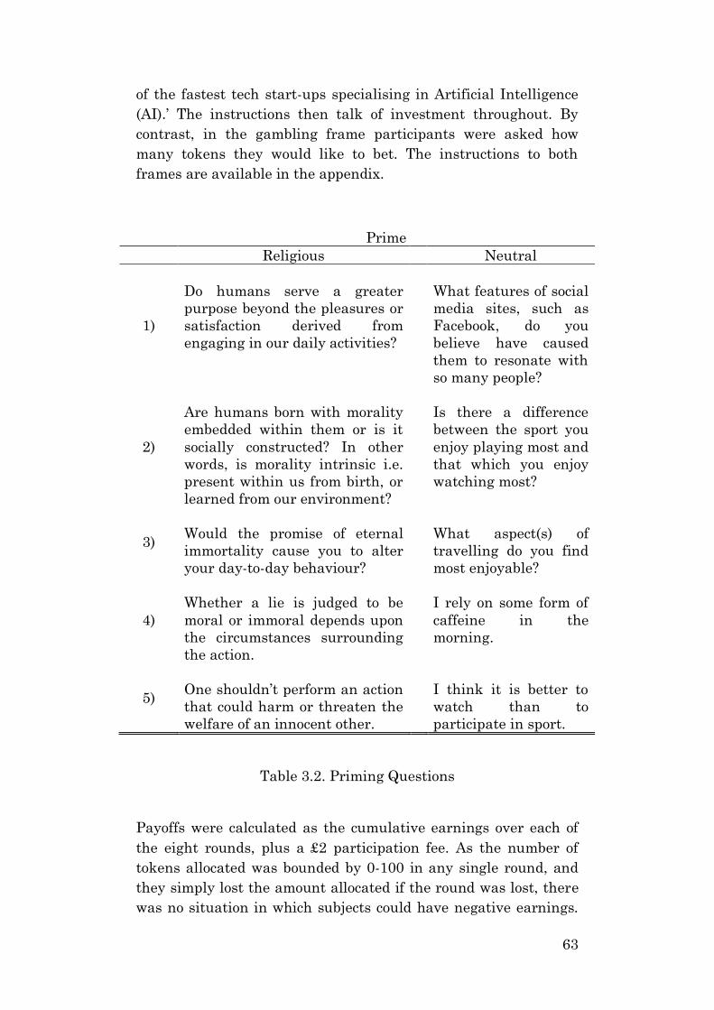
63

of the fastest tech start-ups specialising in Artificial Intelligence

(AI).’ The instructions then talk of investment throughout. By

contrast, in the gambling frame participants were asked how

many tokens they would like to bet. The instructions to both

frames are available in the appendix.

Prime

Religious Neutral

1)

Do humans serve a greater

purpose beyond the pleasures or

satisfaction derived from

engaging in our daily activities?

What features of social

media sites, such as

Facebook, do you

believe have caused

them to resonate with

so many people?

2)

Are humans born with morality

embedded within them or is it

socially constructed? In other

words, is morality intrinsic i.e.

present within us from birth, or

learned from our environment?

Is there a difference

between the sport you

enjoy playing most and

that which you enjoy

watching most?

3)

Would the promise of eternal

immortality cause you to alter

your day-to-day behaviour?

What aspect(s) of

travelling do you find

most enjoyable?

4)

Whether a lie is judged to be

moral or immoral depends upon

the circumstances surrounding

the action.

I rely on some form of

caffeine in the

morning.

5)

One shouldn’t perform an action

that could harm or threaten the

welfare of an innocent other.

I think it is better to

watch than to

participate in sport.

Table 3.2. Priming Questions

Payoffs were calculated as the cumulative earnings over each of

the eight rounds, plus a £2 participation fee. As the number of

tokens allocated was bounded by 0-100 in any single round, and

they simply lost the amount allocated if the round was lost, there

was no situation in which subjects could have negative earnings.

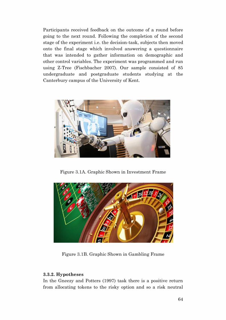
64

Participants received feedback on the outcome of a round before

going to the next round. Following the completion of the second

stage of the experiment i.e. the decision-task, subjects then moved

onto the final stage which involved answering a questionnaire

that was intended to gather information on demographic and

other control variables. The experiment was programmed and run

using Z-Tree (Fischbacher 2007). Our sample consisted of 85

undergraduate and postgraduate students studying at the

Canterbury campus of the University of Kent.

Figure 3.1A. Graphic Shown in Investment Frame

Figure 3.1B. Graphic Shown in Gambling Frame

3.3.2. Hypotheses

In the Gneezy and Potters (1997) task there is a positive return

from allocating tokens to the risky option and so a risk neutral

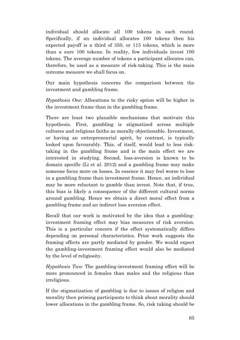
65

individual should allocate all 100 tokens in each round.

Specifically, if an individual allocates 100 tokens then his

expected payoff is a third of 350, or 115 tokens, which is more

than a sure 100 tokens. In reality, few individuals invest 100

tokens. The average number of tokens a participant allocates can,

therefore, be used as a measure of risk-taking. This is the main

outcome measure we shall focus on.

Our main hypothesis concerns the comparison between the

investment and gambling frame.

Hypothesis One: Allocations to the risky option will be higher in

the investment frame than in the gambling frame.

There are least two plausible mechanisms that motivate this

hypothesis. First, gambling is stigmatized across multiple

cultures and religious faiths as morally objectionable. Investment,

or having an entrepreneurial spirit, by contrast, is typically

looked upon favourably. This, of itself, would lead to less risk-

taking in the gambling frame and is the main effect we are

interested in studying. Second, loss-aversion is known to be

domain specific (Li et al. 2012) and a gambling frame may make

someone focus more on losses. In essence it may feel worse to lose

in a gambling frame than investment frame. Hence, an individual

may be more reluctant to gamble than invest. Note that, if true,

this bias is likely a consequence of the different cultural norms

around gambling. Hence we obtain a direct moral effect from a

gambling frame and an indirect loss aversion effect.

Recall that our work is motivated by the idea that a gambling-

investment framing effect may bias measures of risk aversion.

This is a particular concern if the effect systematically differs

depending on personal characteristics. Prior work suggests the

framing effects are partly mediated by gender. We would expect

the gambling-investment framing effect would also be mediated

by the level of religiosity.

Hypothesis Two: The gambling-investment framing effect will be

more pronounced in females than males and the religious than

irreligious.

If the stigmatization of gambling is due to issues of religion and

morality then priming participants to think about morality should

lower allocations in the gambling frame. So, risk taking should be

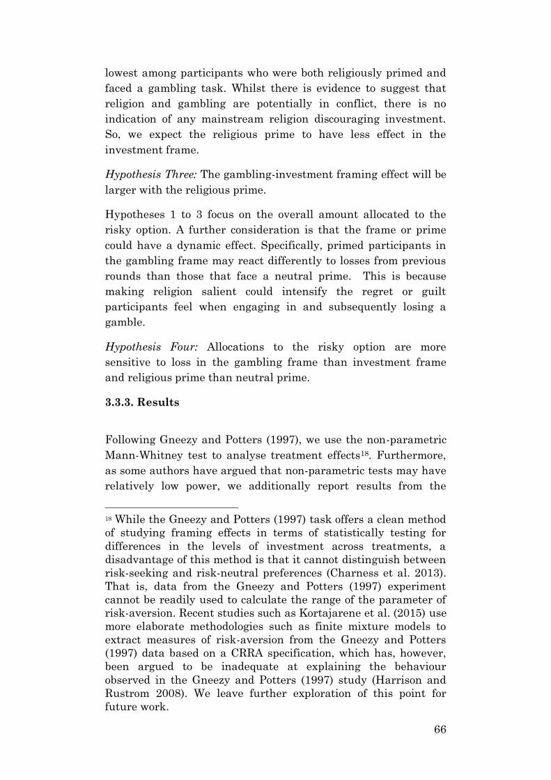
66

lowest among participants who were both religiously primed and

faced a gambling task. Whilst there is evidence to suggest that

religion and gambling are potentially in conflict, there is no

indication of any mainstream religion discouraging investment.

So, we expect the religious prime to have less effect in the

investment frame.

Hypothesis Three: The gambling-investment framing effect will be

larger with the religious prime.

Hypotheses 1 to 3 focus on the overall amount allocated to the

risky option. A further consideration is that the frame or prime

could have a dynamic effect. Specifically, primed participants in

the gambling frame may react differently to losses from previous

rounds than those that face a neutral prime. This is because

making religion salient could intensify the regret or guilt

participants feel when engaging in and subsequently losing a

gamble.

Hypothesis Four: Allocations to the risky option are more

sensitive to loss in the gambling frame than investment frame

and religious prime than neutral prime.

3.3.3. Results

Following Gneezy and Potters (1997), we use the non-parametric

Mann-Whitney test to analyse treatment effects18. Furthermore,

as some authors have argued that non-parametric tests may have

relatively low power, we additionally report results from the

18 While the Gneezy and Potters (1997) task offers a clean method

of studying framing effects in terms of statistically testing for

differences in the levels of investment across treatments, a

disadvantage of this method is that it cannot distinguish between

risk-seeking and risk-neutral preferences (Charness et al. 2013).

That is, data from the Gneezy and Potters (1997) experiment

cannot be readily used to calculate the range of the parameter of

risk-aversion. Recent studies such as Kortajarene et al. (2015) use

more elaborate methodologies such as finite mixture models to

extract measures of risk-aversion from the Gneezy and Potters

(1997) data based on a CRRA specification, which has, however,

been argued to be inadequate at explaining the behaviour

observed in the Gneezy and Potters (1997) study (Harrison and

Rustrom 2008). We leave further exploration of this point for

future work.

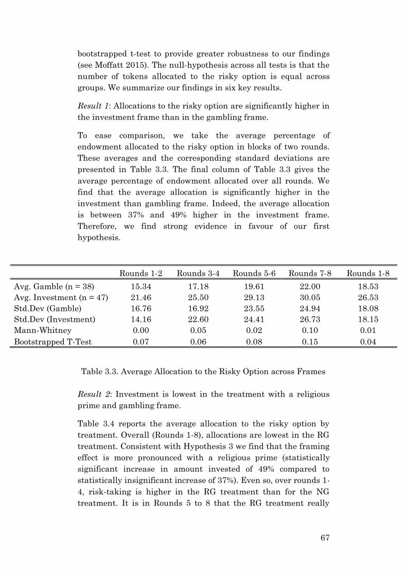
67

bootstrapped t-test to provide greater robustness to our findings

(see Moffatt 2015). The null-hypothesis across all tests is that the

number of tokens allocated to the risky option is equal across

groups. We summarize our findings in six key results.

Result 1: Allocations to the risky option are significantly higher in

the investment frame than in the gambling frame.

To ease comparison, we take the average percentage of

endowment allocated to the risky option in blocks of two rounds.

These averages and the corresponding standard deviations are

presented in Table 3.3. The final column of Table 3.3 gives the

average percentage of endowment allocated over all rounds. We

find that the average allocation is significantly higher in the

investment than gambling frame. Indeed, the average allocation

is between 37% and 49% higher in the investment frame.

Therefore, we find strong evidence in favour of our first

hypothesis.

Table 3.3. Average Allocation to the Risky Option across Frames

Result 2: Investment is lowest in the treatment with a religious

prime and gambling frame.

Table 3.4 reports the average allocation to the risky option by

treatment. Overall (Rounds 1-8), allocations are lowest in the RG

treatment. Consistent with Hypothesis 3 we find that the framing

effect is more pronounced with a religious prime (statistically

significant increase in amount invested of 49% compared to

statistically insignificant increase of 37%). Even so, over rounds 1-

4, risk-taking is higher in the RG treatment than for the NG

treatment. It is in Rounds 5 to 8 that the RG treatment really

Rounds 1-2 Rounds 3-4 Rounds 5-6 Rounds 7-8 Rounds 1-8

Avg. Gamble (n = 38) 15.34 17.18 19.61 22.00 18.53

Avg. Investment (n = 47) 21.46 25.50 29.13 30.05 26.53

Std.Dev (Gamble) 16.76 16.92 23.55 24.94 18.08

Std.Dev (Investment) 14.16 22.60 24.41 26.73 18.15

Mann-Whitney 0.00 0.05 0.02 0.10 0.01

Bootstrapped T-Test 0.07 0.06 0.08 0.15 0.04

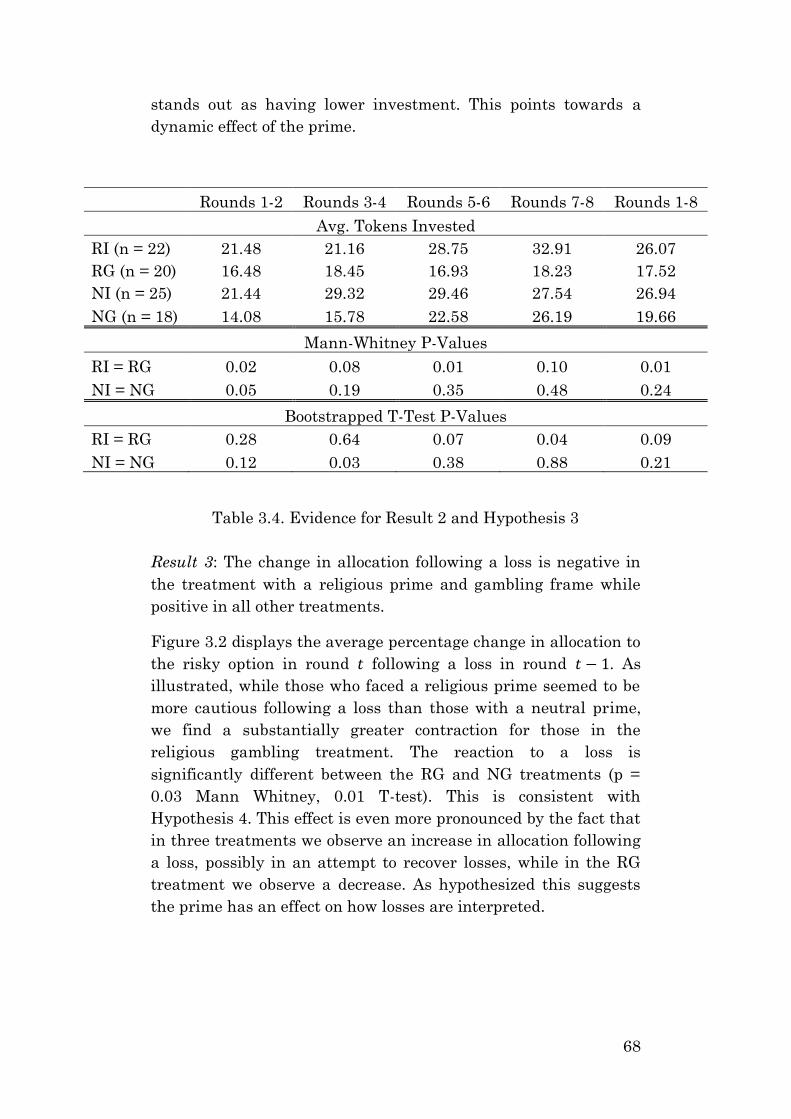
68

stands out as having lower investment. This points towards a

dynamic effect of the prime.


Avg. Tokens Invested

RI (n = 22) 21.48 21.16 28.75 32.91 26.07

RG (n = 20) 16.48 18.45 16.93 18.23 17.52

NI (n = 25) 21.44 29.32 29.46 27.54 26.94

NG (n = 18) 14.08 15.78 22.58 26.19 19.66

Mann-Whitney P-Values

RI = RG 0.02 0.08 0.01 0.10 0.01

NI = NG 0.05 0.19 0.35 0.48 0.24

Bootstrapped T-Test P-Values

RI = RG 0.28 0.64 0.07 0.04 0.09

NI = NG 0.12 0.03 0.38 0.88 0.21

Table 3.4. Evidence for Result 2 and Hypothesis 3

Result 3: The change in allocation following a loss is negative in

the treatment with a religious prime and gambling frame while

positive in all other treatments.

Figure 3.2 displays the average percentage change in allocation to

the risky option in round 𝑡 following a loss in round 𝑡 − 1. As

illustrated, while those who faced a religious prime seemed to be

more cautious following a loss than those with a neutral prime,

we find a substantially greater contraction for those in the

religious gambling treatment. The reaction to a loss is

significantly different between the RG and NG treatments (p =

0.03 Mann Whitney, 0.01 T-test). This is consistent with

Hypothesis 4. This effect is even more pronounced by the fact that

in three treatments we observe an increase in allocation following

a loss, possibly in an attempt to recover losses, while in the RG

treatment we observe a decrease. As hypothesized this suggests

the prime has an effect on how losses are interpreted.

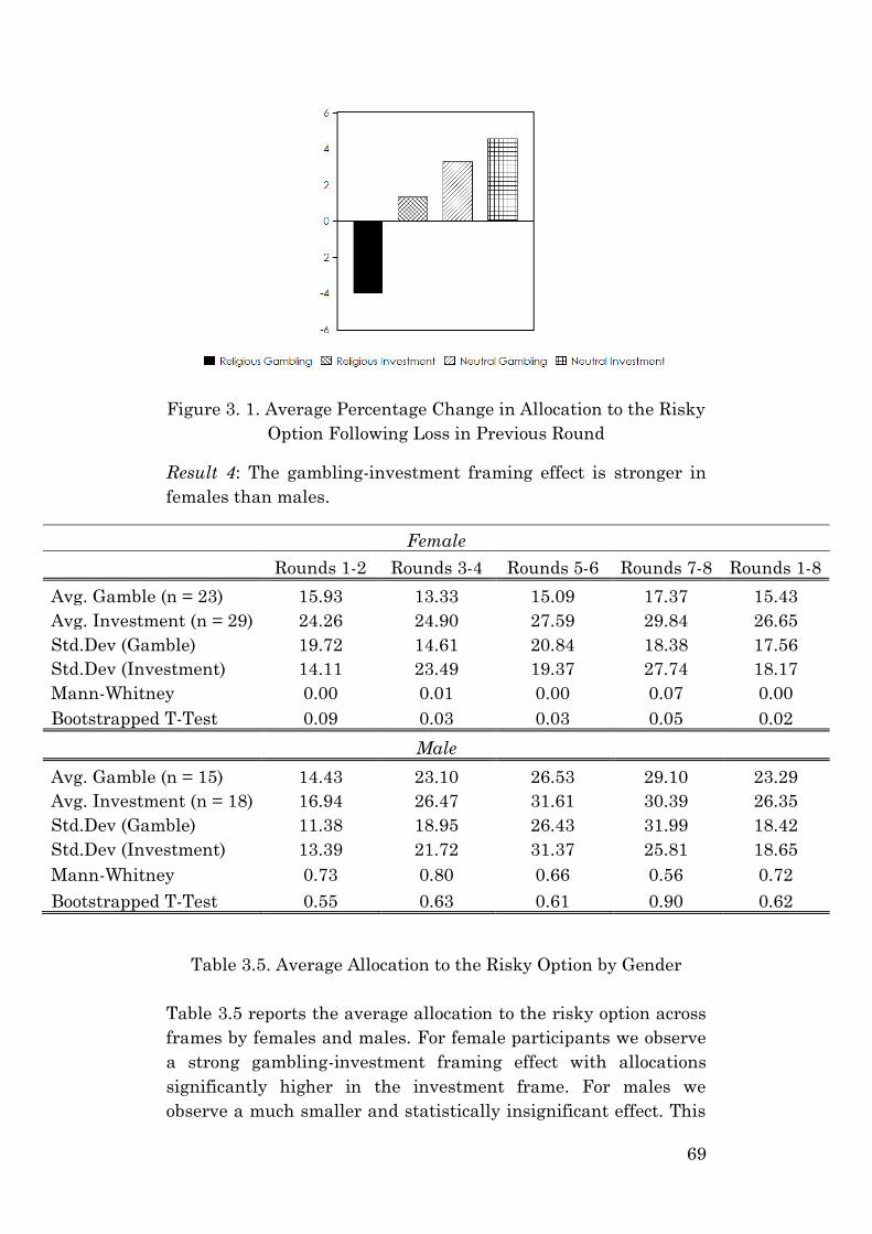
69

Figure 3. 1. Average Percentage Change in Allocation to the Risky

Option Following Loss in Previous Round

Result 4: The gambling-investment framing effect is stronger in

females than males.

Female


Avg. Gamble (n = 23) 15.93 13.33 15.09 17.37 15.43

Avg. Investment (n = 29) 24.26 24.90 27.59 29.84 26.65

Std.Dev (Gamble) 19.72 14.61 20.84 18.38 17.56


Mann-Whitney 0.00 0.01 0.00 0.07 0.00


Male

Avg. Gamble (n = 15) 14.43 23.10 26.53 29.10 23.29

Avg. Investment (n = 18) 16.94 26.47 31.61 30.39 26.35

Std.Dev (Gamble) 11.38 18.95 26.43 31.99 18.42


Mann-Whitney 0.73 0.80 0.66 0.56 0.72


Table 3.5. Average Allocation to the Risky Option by Gender

Table 3.5 reports the average allocation to the risky option across

frames by females and males. For female participants we observe

a strong gambling-investment framing effect with allocations

significantly higher in the investment frame. For males we

observe a much smaller and statistically insignificant effect. This

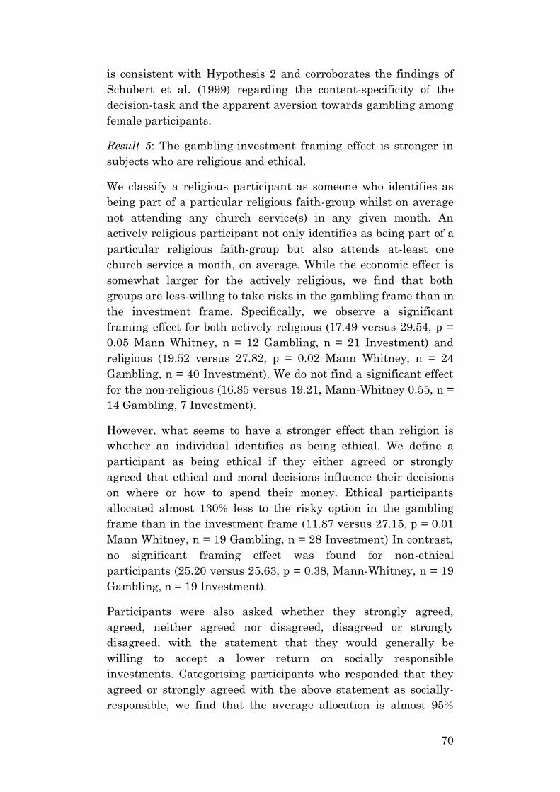
70

is consistent with Hypothesis 2 and corroborates the findings of

Schubert et al. (1999) regarding the content-specificity of the

decision-task and the apparent aversion towards gambling among

female participants.

Result 5: The gambling-investment framing effect is stronger in

subjects who are religious and ethical.

We classify a religious participant as someone who identifies as

being part of a particular religious faith-group whilst on average

not attending any church service(s) in any given month. An

actively religious participant not only identifies as being part of a

particular religious faith-group but also attends at-least one

church service a month, on average. While the economic effect is

somewhat larger for the actively religious, we find that both

groups are less-willing to take risks in the gambling frame than in

the investment frame. Specifically, we observe a significant

framing effect for both actively religious (17.49 versus 29.54, p =

0.05 Mann Whitney, n = 12 Gambling, n = 21 Investment) and

religious (19.52 versus 27.82, p = 0.02 Mann Whitney, n = 24

Gambling, n = 40 Investment). We do not find a significant effect

for the non-religious (16.85 versus 19.21, Mann-Whitney 0.55, n =

14 Gambling, 7 Investment).

However, what seems to have a stronger effect than religion is

whether an individual identifies as being ethical. We define a

participant as being ethical if they either agreed or strongly

agreed that ethical and moral decisions influence their decisions

on where or how to spend their money. Ethical participants

allocated almost 130% less to the risky option in the gambling

frame than in the investment frame (11.87 versus 27.15, p = 0.01

Mann Whitney, n = 19 Gambling, n = 28 Investment) In contrast,

no significant framing effect was found for non-ethical

participants (25.20 versus 25.63, p = 0.38, Mann-Whitney, n = 19

Gambling, n = 19 Investment).

Participants were also asked whether they strongly agreed,

agreed, neither agreed nor disagreed, disagreed or strongly

disagreed, with the statement that they would generally be

willing to accept a lower return on socially responsible

investments. Categorising participants who responded that they

agreed or strongly agreed with the above statement as socially-

responsible, we find that the average allocation is almost 95%

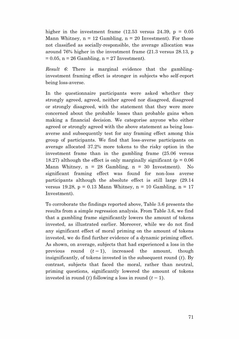
71

higher in the investment frame (12.53 versus 24.39, p = 0.05

Mann Whitney, n = 12 Gambling, n = 20 Investment). For those

not classified as socially-responsible, the average allocation was

around 76% higher in the investment frame (21.3 versus 28.13, p

= 0.05, n = 26 Gambling, n = 27 Investment).

Result 6: There is marginal evidence that the gambling-

investment framing effect is stronger in subjects who self-report

being loss-averse.

In the questionnaire participants were asked whether they

strongly agreed, agreed, neither agreed nor disagreed, disagreed

or strongly disagreed, with the statement that they were more

concerned about the probable losses than probable gains when

making a financial decision. We categorise anyone who either

agreed or strongly agreed with the above statement as being loss-

averse and subsequently test for any framing effect among this

group of participants. We find that loss-averse participants on

average allocated 37.2% more tokens to the risky option in the

investment frame than in the gambling frame (25.06 versus

18.27) although the effect is only marginally significant (p = 0.06

Mann Whitney, n = 28 Gambling, n = 30 Investment). No

significant framing effect was found for non-loss averse

participants although the absolute effect is still large (29.14

versus 19.28, p = 0.13 Mann Whitney, n = 10 Gambling, n = 17

Investment).

To corroborate the findings reported above, Table 3.6 presents the

results from a simple regression analysis. From Table 3.6, we find

that a gambling frame significantly lowers the amount of tokens

invested, as illustrated earlier. Moreover, while we do not find

any significant effect of moral priming on the amount of tokens

invested, we do find further evidence of a dynamic priming effect.

As shown, on average, subjects that had experienced a loss in the

previous round (𝑡 − 1), increased the amount, though

insignificantly, of tokens invested in the subsequent round (𝑡). By

contrast, subjects that faced the moral, rather than neutral,

priming questions, significantly lowered the amount of tokens

invested in round (𝑡) following a loss in round (𝑡 − 1).

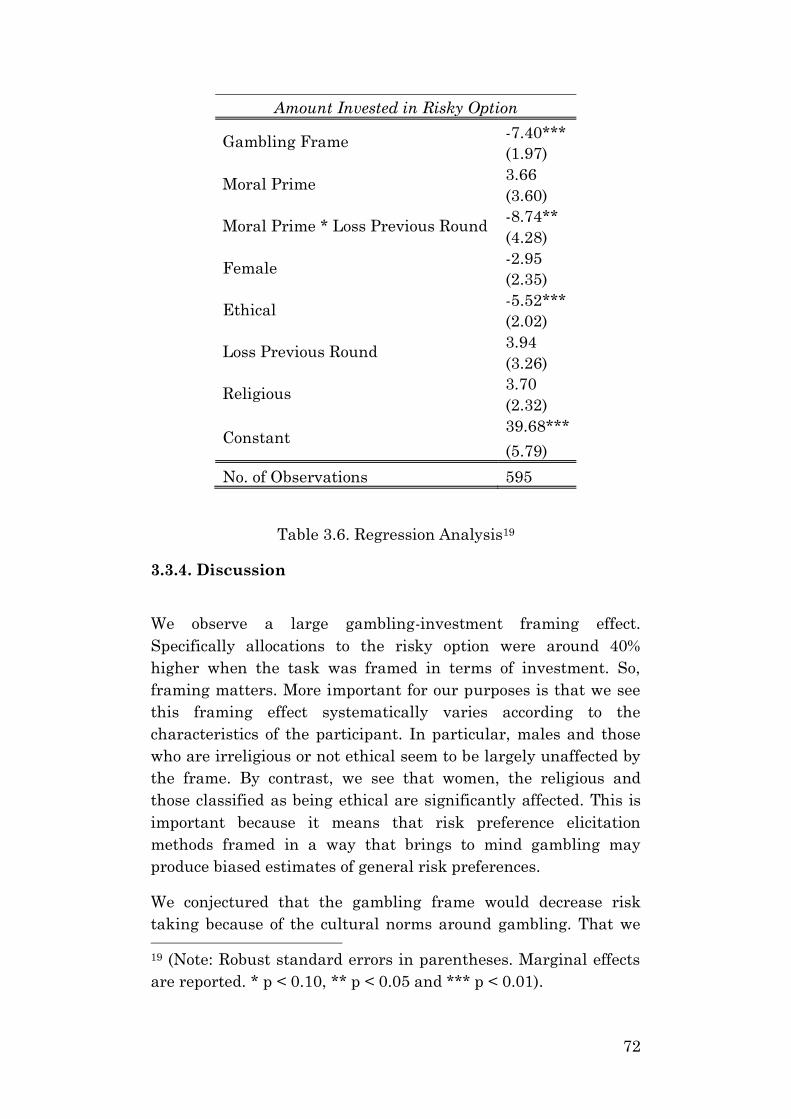
72

Amount Invested in Risky Option

Gambling Frame -7.40***

(1.97)

Moral Prime 3.66

(3.60)

Moral Prime * Loss Previous Round -8.74**

(4.28)

Female -2.95

(2.35)

Ethical -5.52***

(2.02)

Loss Previous Round 3.94

(3.26)

Religious 3.70

(2.32)

Constant 39.68***

(5.79)

No. of Observations 595

Table 3.6. Regression Analysis19

3.3.4. Discussion

We observe a large gambling-investment framing effect.

Specifically allocations to the risky option were around 40%

higher when the task was framed in terms of investment. So,

framing matters. More important for our purposes is that we see

this framing effect systematically varies according to the

characteristics of the participant. In particular, males and those

who are irreligious or not ethical seem to be largely unaffected by

the frame. By contrast, we see that women, the religious and

those classified as being ethical are significantly affected. This is

important because it means that risk preference elicitation

methods framed in a way that brings to mind gambling may

produce biased estimates of general risk preferences.

We conjectured that the gambling frame would decrease risk

taking because of the cultural norms around gambling. That we 19 (Note: Robust standard errors in parentheses. Marginal effects

are reported. * p < 0.10, ** p < 0.05 and *** p < 0.01).

73

observe a bigger framing effect amongst the religious is consistent

with this. It is clear, however, that being religious is not the only

factor. First, we have the gender divide. Second, the correlation

between being ethical and religious among our sample was only

0.14.20 Therefore, it seems as though gambling is deemed

unethical by people beyond those belonging to a particular

religious faith group. This could be because of norms, which have

been shaped by religion, influencing those who are not actively

religious.

We saw that the religious prime primarily had a dynamic effect.

In particular participants exposed to the religious prime

decreased allocation to the risky option if they were exposed to a

loss. This meant that allocations in the treatment where subjects

were exposed to a religious prime and gambling frame was

ultimately significantly lower than in the other three treatments.

Put another way, participants exposed to a neutral prime and

gambling frame increased risk-taking over time. This suggests

that the effects of the frame wore off over time if participants

were not exposed to the religious prime. The prime, therefore, had

a long run impact, potentially by shaping how participants

reacted to outcomes.

3.4. EXPERIMENT 2

Although we find a strong treatment effect for religious

participants in our main experiment, the average gamble is still

positive. If religion prohibits gambling, then it is reasonable to

question why religious participants still decided to bet some

portion of their endowments rather than simply refusing to bet

anything at all. One explanation could be people identify as being

part of a religious faith without actually having too deep an

understanding about the principles or tenets of their chosen

religious ideology. Simply put, religion may serve more as a label

than something which is strictly abided by. This is arguably more

likely to be the case among a sample of university students given

the common finding in the literature that the fervency of religious

20 This falls to 0.10 between those who are ethical and actively

religious.

74

belief declines with education (Inglehart and Baker 2000, Glaeser

and Sacerdote 2008).

Another related explanation is the environment in which

individuals act. That is, behaviour could vary, where individuals

act in a way that is more closely aligned to religious teachings

when they are in a religious or more natural environment. For

instance, university students may decide to gamble when faced

with the task in a laboratory setting but wouldn’t actively decide

to gamble outside of the laboratory. This again could vary

depending on religious intensity. For example, given the

possibility that university students are likely to be less stringent

in their following of religion, they may decide to take a small risk

in the moment whereas those with stricter religious inclinations

may be less willing to do so.

The broader point here is that elicited risk preferences may not

only be subject to the frame and individual characteristics, as

shown in Experiment 1, but also the environment where the

preferences are elicited. To test for such an effect we conducted a

follow-up experiment inside a Mosque, with a control group in a

classroom. Conducting the experiment within the premises of the

Mosque essentially offers a much stronger priming effect as

participants are surrounded by a religious atmosphere. Our main

hypothesis is that we will observe a large framing effect in this

setting.

3.4.1. Methods

To conduct the experiment within the Mosque we condensed

Experiment 1 into a simple one-shot version without the initial

priming questions. Participants simply read the instructions,

made their choice, pulled a number out of a bag to determine

whether they won or not, and then were paid accordingly. This

took around 5 minutes.

The main part of the experiment was conducted inside a Mosque

situated nearby the Canterbury campus of the University of Kent.

Following congregational prayers, an announcement was made

that a research experiment was being conducted in a designated

area of the Mosque. The experiment was conducted in both the

male and female areas of the Mosque to obtain a balanced sample.

We were able to recruit 43 participants.

75

As a control we recruited a further 20 subjects from the general

student population. These participants were exposed to the same

one-shot version of the experiment as those in the Mosque. The

control was carried out in a small lecture theatre at the

university. In both the Mosque and classroom we were careful to

make sure that participants were only exposed to their frame and

could not see the alternative frame.

3.4.2. Hypotheses

Our main hypothesis remains,

Hypothesis One: Risk-taking will be higher in the investment

frame than in the gambling frame.

Here, however, we expect a stronger effect caused by the

particular religious setting and the fact that Islam explicitly

prohibits aleatory transactions such as gambling, wagering or

betting (Schacht 1982). Note that investment is not prohibited

and is positively encouraged in Islam.

Hypothesis five: We will observe a larger framing effect in the

Mosque than in the classroom or Experiment 1.

3.4.3. Results

We summarize our findings in two main results.

Result 7: We observe a very large gambling-investment framing

effect with virtually no gambling in the Mosque.

Table 3.7 presents the average allocation to the risky option by

treatment for participants in the Mosque. Consistent with

Hypothesis 5 we see a very large framing effect. The observed

increase of allocations in the investment frame of 785% compares

to 43.2% in Experiment 1. Moreover, 71.4% of subjects in the

Mosque did not allocate anything to the risky option in the

gambling frame (and 86% gambled with less than three tokens of

their endowment). In contrast, every participant who faced the

investment task allocated a positive amount to the risky option.

Moreover, we observe a large gambling-investment framing effect

for both males and females.

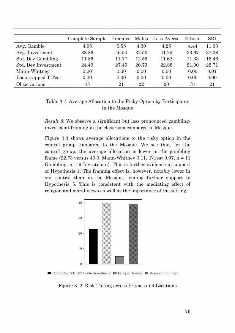
76

Complete Sample Females Males Loss-Averse Ethical SRI

Avg. Gamble 4.95 5.55 4.30 4.25 4.44 11.33

Avg. Investment 38.86 46.50 32.50 41.25 33.67 37.08

Std. Dev Gambling 11.86 11.77 12.56 11.62 11.33 16.46

Std. Dev Investment 24.49 27.49 20.73 22.88 21.00 22.71

Mann-Whitney 0.00 0.00 0.00 0.00 0.00 0.01

Bootstrapped T-Test 0.00 0.00 0.00 0.00 0.00 0.00

Observations 43 21 22 20 31 21

Table 3.7. Average Allocation to the Risky Option by Participants

in the Mosque

Result 8: We observe a significant but less pronounced gambling-

investment framing in the classroom compared to Mosque.

Figure 3.3 shows average allocations to the risky option in the

control group compared to the Mosque. We see that, for the

control group, the average allocation is lower in the gambling

frame (22.73 versus 40.0, Mann-Whitney 0.11, T-Test 0.07, n = 11

Gambling, n = 9 Investment). This is further evidence in support

of Hypothesis 1. The framing effect is, however, notably lower in

our control than in the Mosque, lending further support to

Hypothesis 5. This is consistent with the mediating effect of

religion and moral views as well as the importance of the setting.

Figure 3. 2. Risk-Taking across Frames and Locations

77

3.4.4. Discussion

This experiment reinforces the general point that behaviour is

influenced by the frame, this time in a one-shot setting. The

experiment also powerfully shows that the situational context can

influence the gambling-investment framing effect. Clearly, the

Mosque is a very particular setting with a strong religious

priming effect. Even so, the very large framing effect we observe

illustrates that we can, more generally, expect the setting to

matter. It is particularly noteworthy that we observe a large

framing effect for men as well as women. This compares to

Experiment 1 where the effect was small for men. This nicely

demonstrates that both personal characteristics (male and female

in Experiment 1) and setting (Mosque or lab) influence the

magnitude of the framing effect.

3.5. GENERAL DISCUSSION

Through implementing a simple framing manipulation, we show

that an individual’s propensity to bear risk varies depending on

the framing of the choice they face. This result corroborates the

findings of several earlier studies that provide evidence of the

domain and context-specificity of risk-preferences (MacCrimmon

and Wehrung (1986), Schubert et al. (1999), Weber et al. (2002),

Hanoch et al. (2006), Dohmen et al. (2011)). The significance of

this framing effect varied across demographic groups. Most

notably, female and religious participants displayed a significant

aversion towards gambling, relative to investment. It also varied

across situational settings. For instance, both men and women

showed an aversion to gambling in a Mosque.

Our results add to the literature exploring the often observed

gender disparities across economic domains such as the labor

market (see Blau and Kahn 2000 for a review), and saving,

investment and consumption behaviour (Croson and Gneezy

(2009) and Fisher (2010)). These differences have been

hypothesized to have been driven by gender-specific differences in

preferences (Croson and Gneezy 2009). Several experimental

studies using both real and hypothetical payoffs with either an

explicit or implicit lottery-based framing have consistently found

78

males as being more risk-prone than females (Schubert et al.

(1999), Holt and Laury (2002), Hartog et al. (2002), Eckel and

Grossman (2002) and Charness and Gneezy (2012)). However, if

females are inherently more averse to gambling tasks than males,

as our results indicate, then the results from the aforementioned

studies may not be generalizable beyond the domain of gambling.

Eckel and Grossman (2008), in reviewing the evidence for risk

aversion, conclude that there is no consistent evidence of gender

differences in contextual environments (as opposed to gambling

environments where the evidence is clear). Schubert et al. (1999),

for instance, find that reframing the decision-task as an

investment eliminates the gender-effect that is found when the

problem is presented as an abstract gamble. Similarly, (see Table

3.5) we observe no difference between men and women in an

investment frame but find a significant difference in the gambling

frame. Moreover, in the setting of the Mosque, we find no

difference between men and women in either the investment or

gambling frame. There are contextual frames where females are

more risk averse than men (e.g. Eckel and Grossman 2008b).

Overall, however, we would suggest that the evidence for greater

risk taking in males may well be an artefact of how risk

preferences are elicited.

Evidence of a significant framing effect for religious, ethical and

socially-responsible participants suggests that people take into

account deeper considerations beyond monetary payoffs during

their decision-making process. Understanding differences in risk-

preferences that are derived from cultural or religious

heterogeneity could contribute towards our understanding of

individual differences in socio-economic outcomes (Iannaccone

(1998) and Hoffmann (2013)) such as entrepreneurship decisions

(Audretsch et al. 2007), wealth accumulation (Keister 2003),

savings behaviour (Renneboog and Spaenjers 2012) and labor

market outcomes (Giavazzi et al. 2009). Moreover, if such

differences in individual risk-attitudes are responsible for distinct

economic choices, then they may further provide a microeconomic

foundation for divergent aggregate outcomes21.

21 This has been an area of growing interest, with studies on the

macroeconomic consequences of religion and culture on economic

growth (Barro and McCleary 2003), economic development

79

The existing literature comparing risk-preferences between

religious groups has typically found that Catholics are more risk-

prone than Protestants and that the religious are more risk-

averse than the irreligious (Barsky et al. (1997), Hilary and Hui

(2009), Kumar et al. (2011), Noussair et al. (2012) and Benjamin

et al. (2016)). However, the existing experimental studies have

typically been based around lottery-type tasks. As our findings

show, religious participants are likely to be more sensitive to

framing which resembles gambling. This could explain the

common finding of Protestants being more risk-averse than

Catholics, given the stronger anti-gambling norm among

Protestants, and the religious being more risk-averse than the

irreligious. If participants from particular religious backgrounds

have an unfavourable bias towards gambling whereas non-

religious participants don’t, then similar to the case with gender,

such results may not be reliably generalized to domains beyond

gambling.

In addition to studying framing effects, we also study whether

making religion salient through priming would influence

behaviour. We do not find evidence of the religious prime causing

any difference in risk-taking in terms of the initial investments

made. However, we find that primed participants were more

sensitive to losses i.e. a loss in the previous round led to a sharper

contraction of investment in the subsequent round in comparison

to those with a neutral prime. This effect was strongest for those

given the religious frame which suggests an important dynamic

priming effect. To the best of our knowledge such dynamic effects

have not been considered before. But they are potentially an

important mechanism through which religion can influence

aggregate outcomes.

Let us finish the discussion by clarifying that we are not arguing

gender and religion have no influence on risk attitudes. In our

second experiment we saw a dramatic decrease in the amount

gambled in the Mosque and so religion and religious context

clearly matter. The point we want to make is more that eliciting

risk preferences using a frame involving gambles and lotteries

may give a biased picture. The broader point is that risk

preferences systematically vary depending on individual

(Alesina et al. 2003), governmental systems (La Porta et al. 1999)

and savings and investment ratios (Guiso et al. 2006).

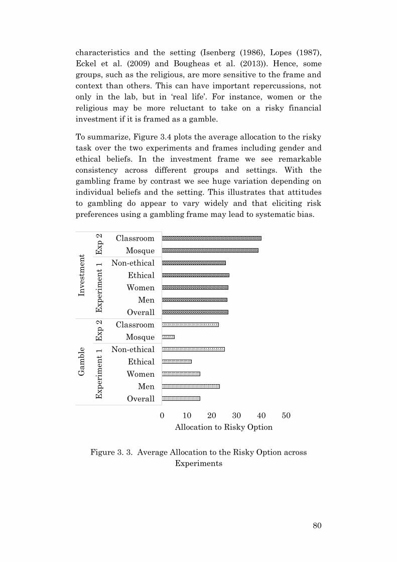
80

characteristics and the setting (Isenberg (1986), Lopes (1987),

Eckel et al. (2009) and Bougheas et al. (2013)). Hence, some

groups, such as the religious, are more sensitive to the frame and

context than others. This can have important repercussions, not

only in the lab, but in ‘real life’. For instance, women or the

religious may be more reluctant to take on a risky financial

investment if it is framed as a gamble.

To summarize, Figure 3.4 plots the average allocation to the risky

task over the two experiments and frames including gender and

ethical beliefs. In the investment frame we see remarkable

consistency across different groups and settings. With the

gambling frame by contrast we see huge variation depending on

individual beliefs and the setting. This illustrates that attitudes

to gambling do appear to vary widely and that eliciting risk

preferences using a gambling frame may lead to systematic bias.

Figure 3. 3. Average Allocation to the Risky Option across

Experiments

0 10 20 30 40 50

Overall

Men

Women

Ethical

Non-ethical

Mosque

Classroom

Overall

Men

Women

Ethical

Non-ethical

Mosque

Classroom

Exp

eri

men

t 1

Exp

2E

xp

eri

men

t 1

Exp

2

Ga

mb

leIn

vest

men

t

Allocation to Risky Option

81


In this study, we ran simple incentivised laboratory experiments

using the seminal Gneezy and Potters (1997) framework to test

whether religious, or ethical, priming and decision-task framing

could influence the appetite for risk among participants. We find

evidence to suggest that reframing an identical numerical

problem into an investment decision results in greater risk-taking

than when it is presented as a gamble. We also find that priming

participants about religion and ethics causes a dynamic effect

where the reaction to losses was stronger for those that were

primed. In our second experiment we find that risk-taking drops

dramatically in the Mosque for those exposed to the gambling

frame.

Overall, our findings corroborate the results of previous studies

that show context is an important determinant of risk-taking

(Schubert et al. (1999), Weber et al. (2002) and Dohmen et al.

(2010)). More specifically, we highlight two conclusions that can

be drawn from our work. First, we find that choices in the

investment frame are relatively stable across personal

characteristics (most notably gender), beliefs (ethical and

religious) and setting (Mosque, lab or classroom) while those in

the gambling frame are not. This suggests that individuals are

particularly sensitive to a gambling frame, potentially because of

the social and religious norms around gambling. Second, we argue

that risk preference elicitation tasks that are framed in terms of

gambling, as many are, likely lead to systematic bias. We should,

therefore, look to test and develop methods that avoid a gambling

frame.

82

3.7. REFERENCES

1. Aflac. (2015). Corporate social responsibility survey report.

2. Ait-Sahalia, Y., and Lo, A.W. (2000). Nonparametric risk-

management and implied risk-aversion. Journal of

Econometrics, 94(1-2), 9-51.

3. Alesina, A., Devleeschauwer, A., Easterly, W., Kurlat, S.

and Wacziarg, R. (2003). Fractionalization. Journal of

Economic Growth, 8(2), 155-194.

4. Andersen, S., Harrison, G.W., Lau, M.I., and Rustrom, E.

(2008). Risk aversion in game shows. In James C.Cox,

Glenn W. Harrison (ed.), Risk Aversion in Experiments,

Research in Experimental Economics, Volume 12, Emerald

Group Publishing Limited, 359-404.

5. Audretsch, D.B., Grilo, I., and Thurik, A.R. (2007).

Explaining entrepreneurship and the role of policy. In D.B.

Audretsch, I. Grilo and A.R. Thurik (Eds.), Handbook of

Entrepreneurship Policy, Cheltenham, Edward Elgar, 1-17.

6. Barro, R.K., and McCleary, R.M. (2003). Religion and

Economic Growth. American Sociological Review, 68, 760-

781.

7. Barsky, R.B., Juster, F.T., Kimball, M.S., and Shapiro,

M.D. (1997). Preference parameters and behavioural

heterogeneity: An experimental approach in the Health and

Retirement study. Quarterly Journal of Economics, 112(2),

537-579.

8. Bartke, S., and Schwarz, R. (2008). Risk-averse by nation

or by religion? Some insights on the determinants of

individual risk-attitudes. SOEP Paper on Multidisciplinary

Panel Data Research, No. 131, Berlin, DIW.

9. Benjamin, D.J., Choi, J.J. and Fisher, G. (2016). Religious

identity and economic behaviour. Review of Economics and

Statistics, 98(4), 617-637.

10. Benjamin, D.J., Choi, J.J., and Strickland, A.J. (2007)

Social identity and preferences. American Economic

Review, 100(4), 1913-1928.

11. Bernoulli, D. (1954). Exposition of a new theory on the

measurement of risk. Econometrica, 22(1), 23-36.

12. Binde, P. (2007). Gambling and religion: Histories of

concord and conflict. Journal of Gambling Issues, 20, 145-

165.

83

13. Blau, F.D., and Kahn, L.M. (2000). Gender differences in

pay. Journal of Economic Perspectives, 14(4), 75-99.

14. Booth, A.L. and Nolen, P. (2012). Gender differences in risk

behaviour: does nurture matter? Economic Journal, Royal

Economic Society, 122(558), 56-78.

15. Bougheas, S., Nieboer, J., and Sefton, M. (2013). Risk-

taking in social settings: Group and peer effects. Journal of

Economic Behaviour and Organization, 92, 273-283.

16. Cabeza, R., Kapur, S., Craik, F.I.M., McIntosh, A.R., Houle,

S., and Tulving, E. (1997). Functional neuroanatomy of

recall and recognition: A PET study on episodic memory.

Journal of Cognitive Neuroscience, 9, 254-265.

17. Charness, G., and Gneezy, U. (2010), Portfolio choice and

risk-attitudes: an experiment. Economic Inquiry, 48(1),

133-146.

18. Charness, G., and Gneezy, U. (2012). Strong evidence for

gender differences in risk-taking. Journal of Economic

Behaviour and Organization, 83, 50-58.

19. Charness, G., Gneezy, U. and Imas, A. (2013).

Experimental methods: eliciting risk preferences. Journal

of Economic Behaviour and Organization, 87, 43-51.

20. Chetty, R. (2006). A new method of estimating risk

aversion. American Economic Review, 96(5), 1821-1834.

21. Cohen, A., and Einav, L. (2007). Estimating risk-

preferences from deductible choices. American Economic

Review, 97(3), 745-788).

22. Croson, R. and Gneezy, U. (2009). Gender differences in

preferences. Journal of Economic Literature, 47(2), 1-27.

23. Dave, C., Eckel, C., Johnson, C., and Rojas, C. (2007). On

the heterogeneity, stability, and validity of risk-preference

measures. Working Paper, University of Texas at Dallas.

24. Deck, C.A., Lee, J., Reyes, J., and Rosen, C. (2010).

Measuring risk-aversion on multiple tasks: Can domain

specific risk attitudes explain apparently inconsistent

behaviour? University of Arkansas, mimeo.

25. Dohmen, T., Falk, A., Huffman, D., Sunde, U., Schupp, J.,

and Wagner, G.G. (2011). Individual risk-attitudes:

measurement, determinants and behavioural consequences.

Journal of the European Economic Association, 9(3), 522-

550.

26. Eckel, C., El-Gamal, M., and Wilson, R. (2009). Risk loving

after the storm: A Bayesian-Network study of Hurricane

84

Katrina evacuees. Journal of Economic Behaviour and

Organization, 69, 110-124.

27. Eckel, C.C., and Grossman, P.J. (2002). Sex differences and

statistical stereotyping in attitudes toward financial risk.

Evolution and Human Behaviour, 23(4), 281-295.

28. Eckel, C.C., and Grossman, P.J. (2008). Men, Women and

risk-aversion: Experimental evidence. Handbook of

Experimental Economics Results, Elsevier.

29. Fischbacher, U. (2007). Z-Tree: Zurich toolbox for ready-

made economic experiments. Experimental Economics,

10(2), 171-178.

30. Fisher, P. (2010). Gender differences in personal saving

behaviours. Journal of Financial Counselling and Planning,

21, 14-24.

31. Giavazzi, F., Schiantarelli, F., and Serafinelli, M. (2009).

Culture, Policies and Labor Market Outcomes. National

Bureau of Economic Research (NBER) Working Paper, No.

154417.

32. Glaeser, E.L., and Sacerdote, B.I. (2008). Education and

religion. Journal of Human Capital, 2(2), 188-215.

33. Glaeser, E.L., Laibson, D.I., Scheinkman, J.A., and Soutter,

C.L. (2000). Measuring trust. The Quarterly Journal of

Economics, 115(3), 811-846.

34. Gneezy, U., and Potters, J. (1997). An experiment on risk-

taking and evaluation periods. Quarterly Journal of

Economics, 122(2), 631-645.

35. Guiso, L., and Paiella, M. (2008), Risk-aversion, wealth,

and background risk. Journal of the European Economic

Association, 6(6), 1109-1150.

36. Guiso, L., Sapienza, P., and Zingales, L. (2006). Does

culture affect economic outcomes? Journal of Economic

Perspectives, 20(2), 23-48.

37. Halek, M, and Eisenhauer, J. (2001). Demography of risk-

aversion. Journal of Risk and Insurance, 68, 1-24.

38. Hanoch, Y., Johnson, J., and Wilke, A. (2006). Domain

specificity in experimental measures and participant

recruitment: An application to risk-taking behaviour.

Psychological Science, 17(4), 300-304.

39. Harrison, G. W., and Rutström, E. (2008). Risk aversion in

the laboratory. In Risk aversion in experiments (pp. 41-

196). Emerald Group Publishing Limited.

85

40. Hartog, J., Ferrer-i-Carbonell, A., and Jonker, N. (2002).

Linking measured risk-aversion to individual

characteristics, Kyklos, 55, 3-26.

41. Hilary, G., and Hui, K.W. (2009). Does religion matter in

corporate decision making in America? Journal of Financial

Economics, 93, 455-473.

42. Hoffman, R. (2013). The Experimental Economics of

Religion. Journal of Economic Surveys, 27(5), 813-845.

43. Holt, C. A., and Laury, S. K. (2014). Assessment and

estimation of risk preferences. In Handbook of the

economics of risk and uncertainty (Vol. 1, pp. 135-201).

North-Holland.

44. Holt, C.A., and Laury S.K. (2002). Risk aversion and

incentive effects. American Economic Review, 92(5), 1644-

1655.

45. Iannacone, L. (1998). Introduction to the Economics or

Religion. Journal of Economic Literature, 36(3), 1465-1495.

46. Inglehart, R., and Baker, W.E. (2000). Modernization,

cultural change and the persistence of traditional values.

American Sociological Review, 65, 19-51.

47. Isaac, R.M., and James, D. (2000), Just who are you calling

risk-averse. Journal of Risk and Uncertainty, 20(2), 177-

187.

48. Isenberg, D. J. (1986). Group polarization: A critical review

and meta-analysis. Journal of Personality and Social

Psychology, 50(6), 1141-1151.

49. Keister, L. (2003). Religion and wealth: The role of religious

affiliation and participation in early adult asset

accumulation. Social Forces, 82, 175-207.

50. Kortajarene, I., Ponti, G. and Lucas., J. (2015). Some

(mis)facts about myopic loss-aversion. Valencian institute

of economic research working paper.

51. Kumar, A., Page, J.K. and Spalt, O.G. (2011). Religious

beliefs, gambling attitudes, and financial market outcomes.

Journal of Financial Economics, 102, 671-708.

52. La Porta, R., Lopez-De-Silanes, F., Shleifer, A., and Vishny,

R. (1999). The quality of government. Journal of Law,

Economics and Organization, 15, 222-279.

53. Lejuez, C.W., Read, J.P., Kahler, C.W., Richards, J.B.,

Ramsey, S.E., Stuart, G.L., and Strong, D.R. (2002).

Evaluation of a behavioural measure of risk taking: the

86

Balloon Analogue Risk Task (BART). Journal of

Experimental Psychology: Applied, 8(2), 75–84.

54. Leon, A.K., and Pfeifer, C. (2013). Religious activity, risk-

taking preferences, and financial behaviour: Empirical

evidence from German survey data. Working Paper Series

in Economics, No. 269, University of Luneburg.

55. Li, Y.J., Kenrick, D.T., Neuberg, S.L., and Griskevicius, V.

(2012). Economic decision biases and fundamental

motivations: how mating and self-protection alter loss-

aversion. Journal of Personality and Social Psychology,

102(3), 550-561.

56. Lopes, L. (1987). Between hope and fear: The psychology of

risk. Advances in Experimental Social Psychology, 20, 255-

295.

57. Lu, J., and Perrigne, I. (2008). Estimating risk-aversion

from ascending and sealed-bid auctions: the case of timber

auction data. Journal of Applied Econometrics, 23(7), 871-

896.

58. MacCrimmon K.R., and Wehrung D.A. (1990).

Characteristics of risk taking executives. Management

Science, 36, 422-435.

59. MacCrimmon, K.R., and Wehrung, D.A. (1986). Taking

risks: The management of uncertainty. Free Press, New

York.

60. Mehra, R., and Prescott, E.C. (1985). The equity premium:

a puzzle. Journal of Monetary Economics, 15(2), 145-161.

61. Miller, A.S., and Hoffman, J.P. (1995). Risk and religion:

An explanation of gender differences in religiosity. Journal

for the Scientific Study of Religion, 34, 63-75.

62. Moffatt, P.G. (2015). Experimetrics: Econometrics for

Experimental Economics. Palgrave MacMillan.

63. Noussair, C. N., Trautmann, S. T., van de Kuilen, G., and

Vellekoop, N. (2012). Risk aversion and religion. CentER

Discussion Paper, Vol. 2012-073, Tilburg, Economics.

64. Post, T., Van den Assem, M.J., Baltussen, G., and Thaler,

R.H. (2008). Deal or no deal? Decision making under risk in

a large-payoff game show. American Economic Review,

98(1), 38-71.

65. Renneboog, L., and Spaenjers, C. (2012). Religion, economic

attitudes and household finance. Oxford Economic Papers,

64, 103-124.

87

66. Schacht, J. (1982). An Introduction to Islamic Law. Oxford

University Press.

67. Schubert, R., Brown, M., and Brachinger, H.W. (1999).

Financial decision-making: Are women really more risk-

averse? American Economic Review, 89(2), 381-385.

68. Szipiro, G.G. (1986). Relative risk-aversion around the

world. Economic Letters, 20(1), 19-21.

69. Weber, E. U., Blais, A.R., and Betz, E. (2002). A domain-

specific risk-attitude scale: measuring risk perceptions and

risk behaviours. Journal of Behavioural Decision Making,

15, 263-290.

70. Weber, E.U., and Hsee, C.K. (1999), Cross-national

differences in risk-preference and lay predictions. Journal

of Behavioural Decision Making, 12, 165-179.

71. Weber, E.U., and Milliman, R. (1997). Perceived risk

attitudes: relating risk perception to risky choice.

Management Science, 43, 122-143.

72. Wheeler, S.C., and Petty, R.E. (2001). The effects of

stereotype activation on behaviour: A review of possible

mechanisms. Psychological Bulletin, 127(6), 797-826.

73. Zuniga, B., and Bouzas, R. (2006). Alcohol consumption

among adolescents: perception of positive and negative

outcomes. Mexican Review of Psychology, 23, 97-110.

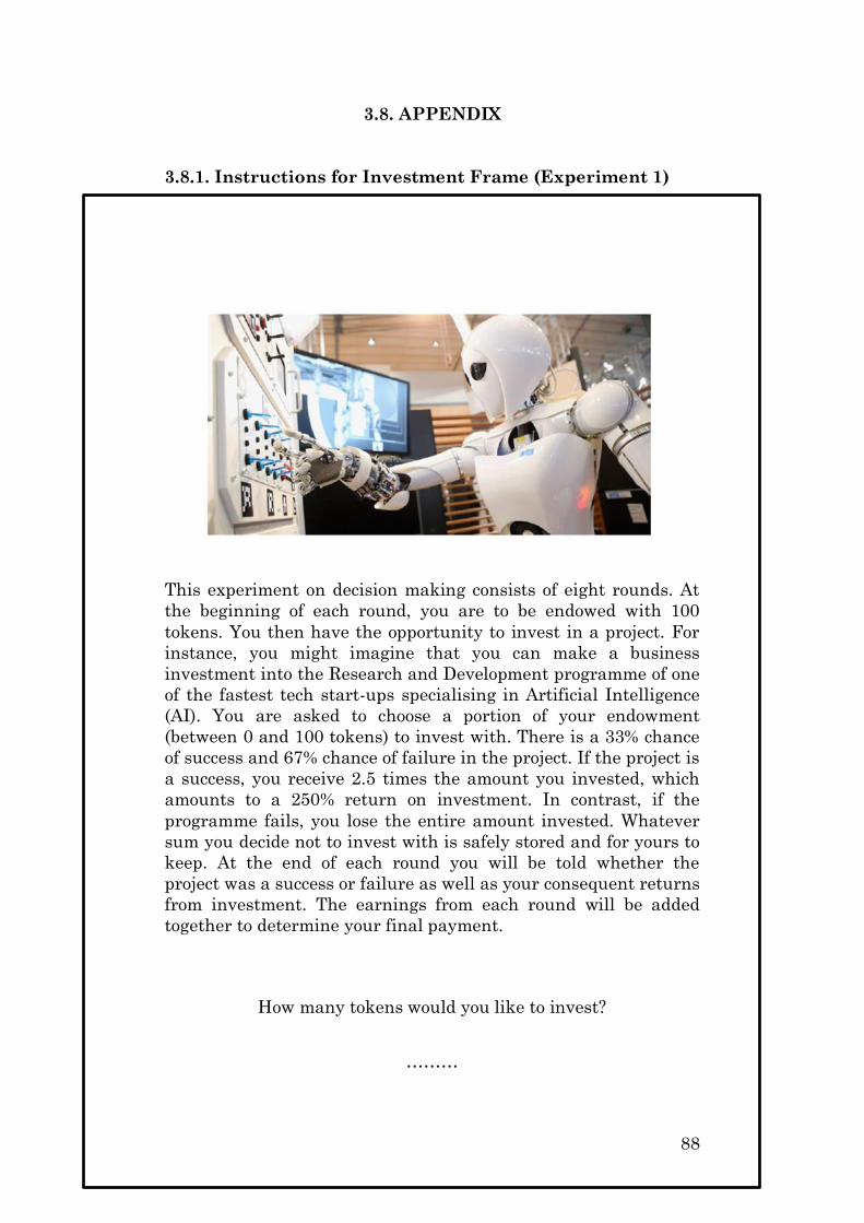
88

3.8. APPENDIX

3.8.1. Instructions for Investment Frame (Experiment 1)

This experiment on decision making consists of eight rounds. At

the beginning of each round, you are to be endowed with 100

tokens. You then have the opportunity to invest in a project. For

instance, you might imagine that you can make a business

investment into the Research and Development programme of one

of the fastest tech start-ups specialising in Artificial Intelligence

(AI). You are asked to choose a portion of your endowment

(between 0 and 100 tokens) to invest with. There is a 33% chance

of success and 67% chance of failure in the project. If the project is

a success, you receive 2.5 times the amount you invested, which

amounts to a 250% return on investment. In contrast, if the

programme fails, you lose the entire amount invested. Whatever

sum you decide not to invest with is safely stored and for yours to

keep. At the end of each round you will be told whether the

project was a success or failure as well as your consequent returns

from investment. The earnings from each round will be added

together to determine your final payment.

How many tokens would you like to invest?

………

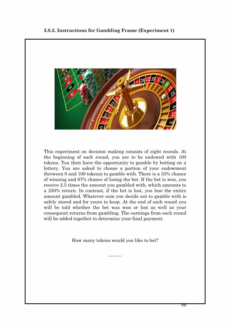
89

3.8.2. Instructions for Gambling Frame (Experiment 1)

This experiment on decision making consists of eight rounds. At

the beginning of each round, you are to be endowed with 100

tokens. You then have the opportunity to gamble by betting on a

lottery. You are asked to choose a portion of your endowment

(between 0 and 100 tokens) to gamble with. There is a 33% chance

of winning and 67% chance of losing the bet. If the bet is won, you

receive 2.5 times the amount you gambled with, which amounts to

a 250% return. In contrast, if the bet is lost, you lose the entire

amount gambled. Whatever sum you decide not to gamble with is

safely stored and for yours to keep. At the end of each round you

will be told whether the bet was won or lost as well as your

consequent returns from gambling. The earnings from each round

will be added together to determine your final payment.

How many tokens would you like to bet?

………

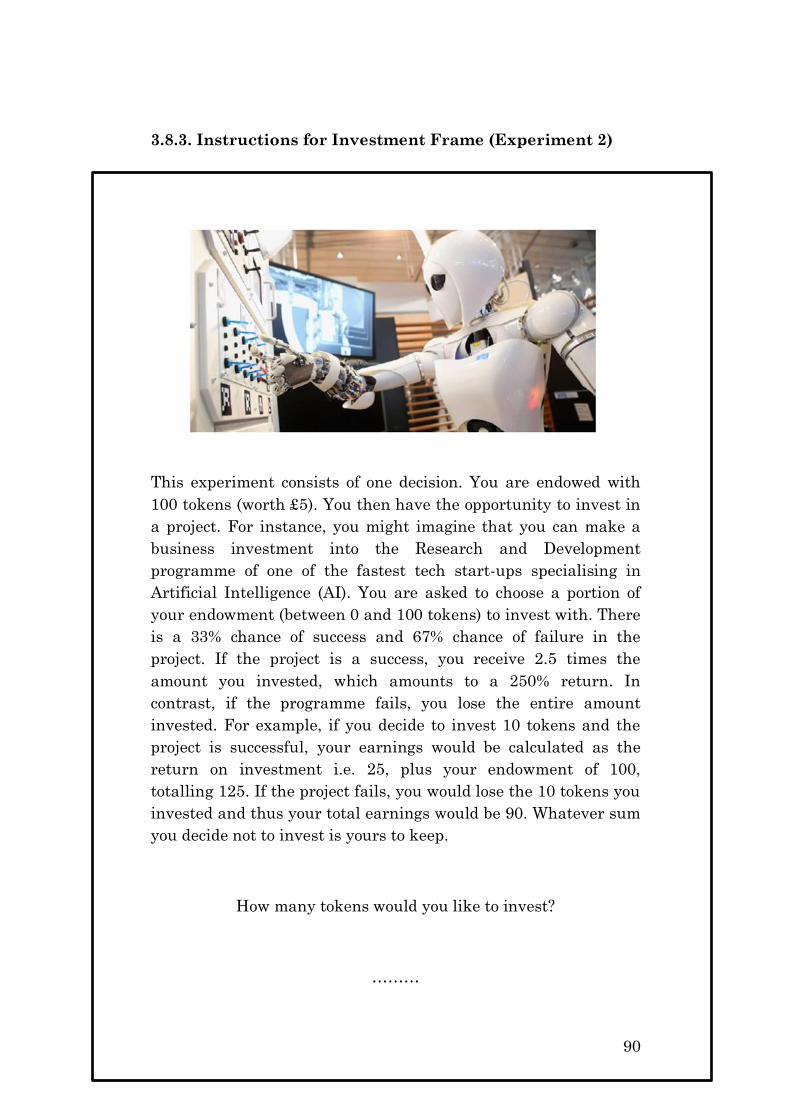
90

3.8.3. Instructions for Investment Frame (Experiment 2)

This experiment consists of one decision. You are endowed with

100 tokens (worth £5). You then have the opportunity to invest in

a project. For instance, you might imagine that you can make a

business investment into the Research and Development

programme of one of the fastest tech start-ups specialising in

Artificial Intelligence (AI). You are asked to choose a portion of

your endowment (between 0 and 100 tokens) to invest with. There

is a 33% chance of success and 67% chance of failure in the

project. If the project is a success, you receive 2.5 times the

amount you invested, which amounts to a 250% return. In

contrast, if the programme fails, you lose the entire amount

invested. For example, if you decide to invest 10 tokens and the

project is successful, your earnings would be calculated as the

return on investment i.e. 25, plus your endowment of 100,

totalling 125. If the project fails, you would lose the 10 tokens you

invested and thus your total earnings would be 90. Whatever sum

you decide not to invest is yours to keep.

How many tokens would you like to invest?

………

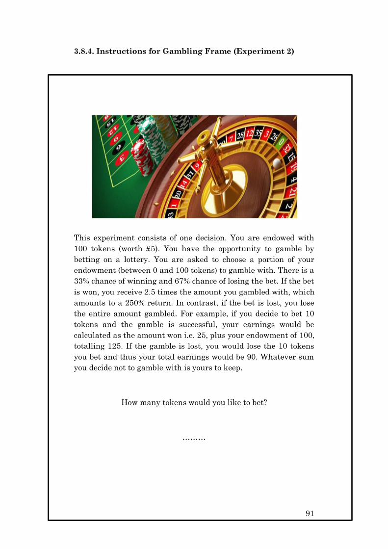
91

3.8.4. Instructions for Gambling Frame (Experiment 2)

This experiment consists of one decision. You are endowed with

100 tokens (worth £5). You have the opportunity to gamble by

betting on a lottery. You are asked to choose a portion of your

endowment (between 0 and 100 tokens) to gamble with. There is a

33% chance of winning and 67% chance of losing the bet. If the bet

is won, you receive 2.5 times the amount you gambled with, which

amounts to a 250% return. In contrast, if the bet is lost, you lose

the entire amount gambled. For example, if you decide to bet 10

tokens and the gamble is successful, your earnings would be

calculated as the amount won i.e. 25, plus your endowment of 100,

totalling 125. If the gamble is lost, you would lose the 10 tokens

you bet and thus your total earnings would be 90. Whatever sum

you decide not to gamble with is yours to keep.

How many tokens would you like to bet?

………

92

CHAPTER FOUR

4. Does Insurance and the Prospect of

Sabotage Crowd Out Prosocial Behaviour?

ABSTRACT

We report the results of a simple laboratory experiment in which

we explore the extent to which altering subject choice-sets and the

context in which the decision is made influences the level of

prosocial and anti-social behaviour among competing individuals.

We find that extending the available choice-set by including the

option to insure crowds out voluntary donations by winners even

when insurance constitutes a dominated strategy. Furthermore,

switching the context of the problem from potentially having one’s

endowment stolen to having it burned by an opponent lowers

prosociality in terms of average donation size. Our data shows

considerable evidence of both sabotage and antisocial behaviour

by contest losers that is consistent across treatments. One

implication of our results is that behaviour can be susceptible to

changes in choice-sets even when the added options do not

represent monetarily advantageous strategies. This provides

further support to the growing consensus on the situational-

instability of preferences.

93

4.1. INTRODUCTION

The economics literature has traditionally focused on the study of

agents with relatively simple self-interested material motivations.

The findings of Smith (1962) illustrated that if subjects trade a

homogenous good of which all aspects are fully contractible then

experimental markets are quick to converge to the competitive

equilibrium. As the equilibrium was computed based on the

assumption that all players were exclusively self-interested, and

the fact that numerous studies successfully corroborated this

result, the findings of Smith (1962) were used to support the

notion that self-interest provided a good description of behaviour

(see Davis and Holt 1993). However, an extensive body of research

based on laboratory experiments has subsequently documented

considerable evidence showing the significance of interdependent

utility, or so-called other-regarding preferences, during the

decision-making process of individuals under various situations,

for purposes such as inequity aversion (Bolton and Ockenfels

(1998), Fehr and Gachter (2000) and Charness and Rabin

(2002))22, altruism (Andreoni and Miller 2002), fairness,

reciprocity (Fehr and Gachter 2000), relative standing

(Kirchsteiger (1994) and Charness and Rabin (2002)), norm-

breaking (Lopez-Perez 2008), social reputation, egocentrism (Cox

et al. 2002) or even spite and envy (Zizzo and Oswald (2001),

Herrmann et al. (2008) Abbink and Sadrieh (2009) and Abbink

and Herrmann (2011)).

Other-regarding preferences have therefore been recognised as

being important for a range of social and economic outcomes, such

as public life and politics (Fehr and Fischbacher 2002), tax-

compliance (Alm et al. 1995), income redistribution (Fong et al.

2005), law enforcement (Lind and Tyler 1988) and workplace

relations (Krueger and Mas 2004).

22 A number of influential economists such as Adam Smith (1759),

Gary Becker (1974), Kenneth Arrow (1981), Paul Samuelson

(1993) and Amartya Sen (1995) had mentioned that individuals

may in fact care about the well-being of others and that this could

potentially have important economic implications.

94

Given the substantial evidence on the existence of interdependent

utility, much of the academic research has now shifted focus

towards developing a deeper understanding of the determinants

and conditions under which these preferences could have

important economic and social implications. For example, despite

the common finding of positive contributions in various public

goods experiments or evidence of sharing in the classical dictator

game, a series of papers have shown that adapting the choice-set

available to subjects can significantly alter their behaviour. List

(2007) and Bardsley (2008) show that extending the dictator game

by allowing dictators to take money from receivers considerably

lowers giving. More generally, differences in the type and extent

of other-regarding behaviour across studies have also been

attributed to issues such as monitoring and anonymity

considerations (Hoffman and McCabe (1994) and Eckel and

Grossman (1996), Bandiera et al. (2005) and Benz and Meier

(2008)), the decision context, self-selection of participants, stake-

sizes, the artificial restriction of choice sets that the lab imposes

and experimenter scrutiny or demand effects (Levitt and List

(2007), Orne (1962), List (2007), Bardsley (2008), Smith (2010),

Oechssler (2010) and Zizzo (2010)), the process that generates the

initial distribution of wealth in these experiments (Cherry et al.

(2002), Rotemberg (2006) and Erkal et al. (2011)), reputational

concerns (List 2006) and the number of decision makers i.e.

unilateral versus bilateral action (Simunovic et al. (2013)).

A particular other-regarding preference that has attracted

growing attention recently is that relating to antisocial behaviour,

which is based upon negative utility interdependence. Antisocial

behaviour is now being recognized as an important social and

economic problem in the real world. There is an abundance of

examples that showcase the existence of such behaviour within

everyday life, such as littering, graffiti, vandalism, damaging

private properties, theft, bullying, harassment, cyber-crime,

viruses and malware. According to the British Crime Survey

(2016), around 1.8m incidents of antisocial behaviour were

recorded by police between 2012 and 2013. Since data on

antisocial behaviour is restricted to those incidents that have

been reported, the actual number of incidents is likely to be

higher than what has been reported.

95

These actions impose not only private costs upon those that are

directly affected, but also external or third-party costs to society.

In an attempt to quantify such costs, Cohen (1998) estimated that

a typical career criminal causes around $1.3m to $1.5m in

external costs to society. The corresponding figure for heavy drug-

users was between $370,000 and $970,000. Overall, Cohen’s

(1998) calculations suggest that the monetary value of saving a

high-risk youth from such lifestyle would be in the region of

$1.7m to $2.3m.

To provide a more concrete perspective of the costs associated

with antisocial behaviour, data from the UK shows that

government agencies in England and Wales spend around £3.4m

a year in responding to reports of antisocial behaviour. In 2003,

the Home Office formed the antisocial behavioural unit with an

annual budget of £25m to design and implement the

Government’s policy on antisocial behaviour (HoC 2007). Clearly

then, understanding what drives individuals to carry out such

actions has serious real-world applications.

This chapter contributes towards the literature on social-

preferences and other-regarding utility in the following ways.

First, while previous studies focus on studying whether

individuals are willing to give or take money under various

settings, we further test whether people are sufficiently concerned

about the possibility of others taking or sabotaging their earnings

and as a result willing to invest resources to avoid this. More

specifically, in our no insurance treatments we allow subjects to

simultaneously transfer i.e. give or take money from an opponent

at a fixed cost, or do nothing. We then introduce a treatment

whereby the available choice-set is extended to include the option

of purchasing insurance against the risk of subjects having money

taken away from them. This allows us to test how changes in the

available choice-set influences behaviour.

Secondly, given the recent growth in interest regarding anti-social

behaviour within the lab, we study whether the decision to take

from an opponent is influenced by whether the amount taken is

kept or burned. Zizzo and Oswald (2001) found that 62.5% of

participants chose to burn their opponents’ money in an

incentivised experiment despite the fact that such a decision

implied a net monetary cost to them. Importantly, Zizzo and

Oswald (2001) created the initial allocation of funds across

96

subjects through a betting stage, which was followed by the

random endowment of arbitrary gifts to some participants in

order to provide them with an unfair advantage. As this was

common knowledge, the authors argue that the fundamental

driver of burning was inequity aversion and subjects’ dislike for

the unfairness involved in the process.

Given that there is a robust finding within the experimental

literature showing that behaviour varies depending on the way in

which the initial distribution of wealth is generated (e.g. Durante

et al. (2014) and Akbas et al. (2014)), our experimental design

further involves subjects initially participating in a winner-takes-

all competition in order to earn their endowments. The

competition was set up so that half of the subjects received ‘easier’

questions, which means that the allocation of endowments was

essentially exogenous. Even so, subjects may have felt as though

they ‘earned’ their endowment. If individuals believe that

inequality reflects differences in effort as opposed to luck or

privilege, this may affect their willingness to redistribute

(Durante et al. 2014). Prior literature has shown that other-

regarding behaviour is mitigated when participants earn their

endowments (see Hoffman and Spitzer (1985), Hoffman et al.

(1994), Ruffle (1998), Cherry et al. (2002) and Carpenter et al.

(2010)). For instance, Erkal et al. (2011) show that after

competing in an experimental tournament, those ranked first are

significantly less likely to redistribute their earnings compared to

those of any other rank.

Furthermore, by allowing subjects in our experiment to give, take,

do-nothing and, in a particular treatment, purchase insurance, we

arguably provide subjects with a more complete choice-set to

choose from. This could aid in our understanding of how

individual’s behave when they are faced with a more realistic

scenario that consists of multiple possible options rather than a

simple binary choice, which may be relatively more prone to

experimenter demand effects.

Therefore, the combination of offering subjects a broader choice-

set, the existence of an effort stage and the strategic concerns

created by the bilateral design of our experiment i.e. simultaneous

action by subjects, could offer valuable insights into the stability

or dynamics of social preferences under a setting that is different

from what has been covered in the earlier literature.

97

4.2. FURTHER RELATED LITERATURE

As alluded to above, a plethora of studies have found evidence in

support of the existence of other-regarding preferences. The

literature on social-preferences has traditionally placed greater

emphasis on studying pro-social behaviour. That is, voluntary

behaviour intended to benefit others through actions such as

sharing, donating and co-operating for reasons such as warm

glow, prestige, fairness, social pressure and philanthropy (see

Brown, Meer and Williams 2012). For example, it has been found

that in the classical dictator game, where an individual decides

what proportion of a monetary endowment they would like to

share with an anonymous person, people often violate traditional

assumptions of self-interest by making positive transfers to the

other player. This is despite the fact that the other player is

simply a passive participant who cannot punish the dictator for

not sharing the endowment (see Engel 2011 for a review). Several

extensions have been made to the traditional dictator game to

find evidence of how reducing dictator-recipient social distance

and increasing emotional feelings towards the recipient can

increase giving (see Eckel and Grossman (1996), Hoffman et al.

(1996), Bohnet and Frey (1999) and Branas-Garza et al. (2012)).

More recently, there has been a growing interest in exploring the

so-called darker or negative departures from the customary

assumption of rational self-interest. Research on anti-social

preferences looks into the willingness of individuals to make

others worse off for reasons such as inequality-aversion, envy,

spite and even pure nastiness. The established literature shows

that subjects are in fact willing to behave antisocially even if this

implies that they must incur a net monetary cost in doing so (e.g.

Zizzo and Oswald (2001) and Abbink and Sadrieh (2009)).

While the experimental research on anti-social behaviour is very

limited, researchers have argued that a supposed “homo-rivalis”

or “homo-maliciosus” (Herrmann and Orzen 2008) may provide

better explanations for various social dilemmas in comparison to

the standard homo-economicus. For example, if attitudes towards

income redistribution were purely based on rational self-interest,

then anyone earning less than the average level of income should

98

favour redistribution, since they would benefit from such a policy.

That is, an increase in income inequality skews the distribution of

income rightwards. Therefore, as inequality increases, a larger

share of the population has income beneath the mean, which

implies that the support for redistribution should rise. However,

empirically this hasn’t been the case. For instance, Kuziemko et

al. (2014) find that agents exhibit last place aversion. This result

holds across both laboratory settings and in everyday social

environments. People near the bottom of the income distribution

oppose redistribution due to fears that it could result in people

below them catching up or even overtaking them and thus leave

them at the bottom of the status hierarchy.

Muller et al. (2016) argue that antisocial preferences appear to be

linked to resource scarcity and competition pressures. In other

words, antisocial preferences follow an evolutionary logic similar

to that found across nature. That is, by harming others, one may

be able to reduce competition and therefore such behaviour should

co-vary with competition intensity. This would be analogous to

bacteria that release toxins to kill closely-related species (Muller

et al. 2016). If this is indeed the case then trends in wage

stagnation and anaemic long-term economic growth in certain

parts of the world could increase competition pressures and make

antisocial preferences a lot more important to understand.

The research on anti-social preferences within the realm of

experimental economics was initiated in a seminal paper by Zizzo

and Oswald (2001). In their study, Zizzo and Oswald (2001)

introduce a one-shot version of the money burning game, which

follows a simple two-stage process. In the first stage, the authors

create a wealth distribution among participants through having

them engage in a betting game. However, some subjects receive

an arbitrary gift, which provides them with an unfair advantage

over other participants. These gifts, which boost their recipients’

endowment, were public knowledge in that all participants were

both aware of this feature of the game and the exact amounts

allocated or given to these more fortunate players.

Subsequent to this initial betting stage, subjects were then

allowed to burn i.e. reduce the money-holdings of other subjects,

under complete anonymity, for a given price. Zizzo and Oswald

(2001) vary this price or cost of burning to gauge the extent of

negative utility interdependence between subjects. In other

99

words, to assess how the amount of burning varies with the cost of

burning.

Given the set-up of their experiment, standard economic

assumptions would predict there to be no burning given that

burning here incurs an own cost for no material benefit in return.

However, the authors find substantial evidence of burning. More

precisely, they report that 62.5% of participants chose to burn

despite the fact that such a decision implied a net monetary cost

to them. Furthermore, on average each subject had 48.7% of their

earnings burnt.

While Zizzo and Oswald (2001) don’t find any significant

correlation between the price of burning and the decision to burn,

they do find evidence suggesting that the rationale behind most of

the burning was driven by whether or not the money had been

received deservedly or otherwise. Therefore, rather than the

burning being driven purely by spite or envy, they argue that

money was burned primarily due to concerns for fairness as

participants appeared to use the information regarding unearned

gifts in making their decisions on whether or not to burn.

In a subsequent paper, Zizzo (2004) extends the design of Zizzo

and Oswald (2001) to provide a more focused analysis on whether

agents indeed take into consideration distributional and

procedural fairness when making decisions on burning the

money-holdings of other participants, as indicated in Zizzo and

Oswald (2001). In the new set-up, Zizzo (2004) gives agents the

ability to change the wealth distribution by paying to reduce and

redistribute the money of other participants. Furthermore, half of

the sessions included the possibility of stealing from others.

Standard economic assumptions would suggest that self-

interested agents should do nothing in the non-stealing condition,

since this would imply a net-cost to them, and that they should

steal everything from everybody in the stealing condition. Zizzo

(2004) reports substantial evidence of stealing when it is allowed

but notes that this is always much lower than 100%. However,

Zizzo (2004) argues that this is unlikely to be purely motivated by

self-interest as moving from the stealing to non-stealing condition

increases burning rates. More precisely, the burning ratio is only

8% when stealing is allowed compared to an average of 20% in the

non-stealing setting. Therefore, since burning appears to be an

imperfect substitute for stealing, some stealing is likely to have

100

been motivated by negative utility interdependence but some

burning may have stemmed from a good motive, namely the

aversion to unfairness.

In order to isolate anti-social behaviour stemming from pure envy

and spite rather than any pecuniary, fairness or reciprocity type

motives, Abbink and Sadrieh (2009) introduce the joy-of-

destruction game. The game has two stages. First, two players

earn an endowment, which is equal in expectation, through the

completion of some tasks. Subsequent to this, both players can

then mutually and simultaneously destroy each other’s

endowments. Destruction is costless and entails no material

benefit for the destroying party, and thus the presence of

destruction would provide stronger evidence of pure spite and

nastiness among participants. Abbink and Sadrieh (2009) use a

repeated interaction framework to observe the dynamics of play.

For example, whether the opportunity to retaliate could trigger

the escalation into an ongoing vendetta or perhaps have a

deterrent effect. Furthermore, the authors use two variants of the

game. In the “open” treatment, destruction is perfectly observable

after the completion of each round. In the “hidden” treatment, the

destruction is veiled by an additional random destruction. That is,

in the hidden setting, there is some positive probability that the

endowment of agents is destroyed by “nature.” However, the

targeted individual can only observe the total damage to their

endowment and cannot identify its source. Hence, in this

treatment it became possible to damage someone’s endowment

under anonymity.

Similar to the experiments by Zizzo and Oswald (2001) and Zizzo

(2004), standard economic assumptions would predict there to be

no destruction. The authors find that the overall frequency of

destruction is on average 8.5% of all decisions made under the

open treatment. Furthermore, they observe that destruction rates

are higher in the earlier rounds but are quick to fade away.

However, in the hidden treatment, an average of 39.4% of all

decisions involved destruction. Also, unlike the open treatment,

they find no evidence of destruction rates falling over subsequent

periods.

Abbink and Herrmann (2011) use a one-shot version of the joy-of-

destruction game whereby two players are given equal

endowments and subsequently engage in the simultaneous

101

decision on whether or not to reduce the payoff of the other player

by incurring an own cost. Similar to Abbink and Sadrieh (2009)

the authors use an open and hidden treatment where there exists

some positive probability that nature would partly destroy the

opponent’s endowment.

Abbink and Herrmann (2011) argue that the hidden feature

should increase burning rates. This is because if nature were to

destroy part of the opponent’s income, then it could perhaps lower

the moral costs of burning. In other words, if there is a chance

that the target loses their money anyway, and the source of this

loss isn’t identifiable, then the scruples subjects have to harm

other subjects are reduced, and thus they could become

considerably nastier. While the findings do show that burning

rates are higher in the hidden treatment, at 10.8%, their

explanation seems debatable. More precisely, if one knows that

another person could be inflicted with punishment, this could

actually elicit feelings of greater sympathy towards such an

individual and thus increase the moral costs of imposing further

harm upon them.

Karakostas and Zizzo (2016) extended the joy-of-destruction game

used by Abbink and Herrmann (2011) to study the role of

experimenter demand effects. Karakostas and Zizzo (2016) found

that 60% of subjects chose to reduce their opponent’s earnings

when an indirect yet unequivocal cue to destroy was given to

them. The authors argue that compliance norms and social image

towards the authority can be influential in determining the

choices individuals decide to make.

Abbink and Herrmann (2009) design the vendetta game to

investigate antisocial preferences and conflict. In this game, two

groups of four players interact with each other over ten identical

rounds. In every round, each player receives an equal endowment

and subsequently decides on whether or not they would like to

pay to reduce the payoff of members of the other group. Lowering

the other group’s payoff would entail no material benefit for the

destroyer or their group but would in fact lower their own

monetary earnings. Therefore, any evidence of burning could be

interpreted as purely representing antisocial behaviour. The

authors also add an additional treatment whereby they include an

incentive to destroy money. This takes the form of a prize draw

where one out of however many members of a particular group

102

that decided to burn could win a prize of five points. However, this

prize is lower than the fixed cost of burning and thus still implies

a net cost to the participant in monetary terms. Abbink and

Herrmann (2009) argue that this treatment could mirror symbolic

rewards from committing destructive acts such as social prestige

or honour, and could perhaps incentivise or nudge those more

inclined but hesitant to destroy towards doing so. The authors

find that the introduction of a symbolic reward increases the

frequency of hostile acts to an average of 40% over the ten rounds

compared with 13% in their baseline treatment. However, both

treatments displayed similar dynamics of play. Specifically,

although destruction rates remained significantly higher in the

prize treatment throughout the experiment, these rates seemed to

drop across both treatments after the first two periods, which

could be attributed to the fear of retaliation.

Abbink, Masclet and Van-Veelen (2011) provide the first study on

the role of framing when studying anti-social preferences. That is,

to explore the influence of context, the authors reframe the simple

money-burning task by altering the domain from that of gains to

that of losses. For example, in the treatment representing losses,

the question was framed as an option of paying to reduce the

opponent’s payoff whereas in the second treatment, the same task

was framed as an option of being paid to increase the opponent’s

payoff.

Furthermore, Abbink, Masclet and Van-Veelen (2011) adjust the

initial endowments of the participants to study whether starting

from a point of advantageous or disadvantageous inequality had

any impact on the decision to burn. While the authors find similar

destruction rates overall, with burning taking place on average in

25.2% of cases within the negative framing framework and 24% in

the positive framework, they find differences in the behavioural

patterns of participants. More precisely, within the negative

framing setting, they find that subjects exhibit equity aversion

rather than inequity aversion, while in the positive setting, the

relationship between advantageous and disadvantageous

inequality is reversed. That is, while antisocial behaviour in the

negative setting is seemingly being driven by what the authors

argue is aggressive competitiveness i.e. the wish to enhance an

already advantageous position; they find that in the positive

103

frame, antisocial behaviour is driven by the desire to close an

unfavourable income gap.

Kessler, Ruiz-Martos and Skuse (2012) conduct a one-shot

experiment with the destructor game. In this game, subjects first

earn an endowment based on the completion of some tasks.

Following this, participants are randomly paired and assigned the

roles of a destructor and a passive subject. Each destructor then

decides the percentage of their passive partner’s earnings to

destroy, with destruction being costless and hidden. In order to

exclude inequity and equity aversion motives for destruction, only

1000 tokens earned from the initial tasks were vulnerable for

destruction, with the total earnings of the passive subject

remaining hidden. Each destructor could choose to destroy either

0%, 20% or 40% of the passive players endowment of 1000 tokens.

Furthermore, for 20% of all passive players, “nature” destroys

either 20% or 40% of the endowment, with equal probability.

However, with the maximum destruction inflicted upon any

passive participant capped at 40%, if both destructor and nature

chose to destroy 40% of the passive player’s earnings, then

nature’s destruction would be ineffective.

Using a large sample of 1212 students, the authors find that

15.5% of destructors chose to destroy their passive partner’s

endowment. Specifically, 8.7% of destructors destroyed 20% and

6.8% destroyed the maximum possible 40% of their partner’s

endowment. Following the experiment, participants were asked to

complete various personality-related questionnaires on

neuroticism and psychopathy. From this data, Kessler, Ruiz-

Martos and Skuse (2012) find that destructive behaviour isn’t

significantly associated to any particular personality or

psychopathic characteristics.

In a seminal study, Herrmann et al. (2008) document the

widespread existence of antisocial punishment, which they define

as the sanctioning of people who behave pro-socially. Using a

public goods experiment with the added possibility of punishing

group members, they investigate how an individual who has

contributed a given amount to the public good punishes group

members who either contributed less, the same amount or more

than them. Importantly, the authors also study how this decision

varies across cultural settings. Using a large sample of 1120

undergraduate students who then act in an identical environment

104

i.e. a laboratory setting, the authors find considerable and

significant cross-societal heterogeneity in terms of differences in

cooperation levels and anti-social punishment. For instance, while

some participant pools showed little evidence of antisocial

punishment, others seemed to punish those behaving more pro-

socially than themselves as harshly as they did free-riders.

Furthermore, contributions were highly and significantly

different across pools, with the most co-operative pool

contributing on average 90% of their endowment, which was 3.1

times higher than the least co-operative pool, with an average of

29%. Moreover, not only do Herrmann et al. (2008) find

differences in punishment, but they also find differences in how

participants react to punishment. That is, while punishment had

an efficiency enhancing property in certain pools, in that it

induced free-riders to increase contributions, participants from

some pools took punishment a lot more negatively, which resulted

in an increase in anti-social punishment. The authors argue that

this is likely due to the way in which punishment is perceived

across different cultures, with some reacting positively by

increasing contributions and others seeking out revenge.

Fehr (2018) studies whether increasing inequality causes an

increase in antisocial behaviour towards others. Subjects were

randomly matched into groups of four and subsequently took part

in a task to earn money. Fehr (2018) implements two treatments

which involve paying a bonus to the highest performing member

and allowing members to cheat by paying to artificially increase

their performance before their scores are revealed. Following the

completion of this task, subjects were given information regarding

their performance relative to other group members and were

given the opportunity to pay to burn up to half of the income of

another group member. Only the decision of one randomly

selected group member was implemented. Fehr (2018) finds

evidence to suggest that the extent of antisocial behaviour

depends upon whether the increase in inequality can be

attributed to effort and how transparent the cause of the

inequality was.

To summarise, previous studies have found evidence of both

prosocial and anti-social behaviour within a lab-setting. As

described above, the existence of such preferences has typically

been tested by presenting subjects with narrow choice-sets such

105

as the binary choice of either doing nothing or burning an

opponent’s endowment. Under such a setting, evidence of burning

would then be used in support of the proposition that agents do

exhibit antisocial preferences. Moreover, a growing strand of

literature has shown that the preferences and decisions of agents

are in general sensitive to changes in the context and situation in

which they are made. Our study contributes to the existing

literature in a few ways.

First, we attempt to mitigate any potential experimenter demand

effects by offering subjects a broader choice-set which includes the

option to give, take, do nothing and insure. In other words, if the

decision to be made by subjects involves two options i.e. to steal

money or do nothing, then this could act as a cue as to what

constitutes appropriate behaviour within the experimental setting

and thus influence the behaviour of subjects (see Zizzo 2010).

Therefore, framing the question more naturally by allowing

subjects the option to give, take, do nothing, insure, as well as

implementing an initial effort stage whereby subjects may feel as

though the endowment is earned rather than arbitrarily allocated,

could arguably bring behaviour into closer alignment with a

subject’s true preferences.

The main area of novelty in our experiment lies in the

introduction of an option for subject’s to purchase insurance.

Allowing subjects to insure could provide insight not only into

whether there is a shift towards insuring and the determinants of

insurance demand, particularly when insurance is a dominated

strategy in monetary terms, but also how this impacts the extent

to which subjects choose the other three options available to them.

More precisely, as subjects in our experiment can only choose one

option i.e. give, take, do nothing or insure (in the insurance

treatment), it is of interest to examine whether the shift towards

insurance is driven by a reduction in taking, the choice to do

nothing or the crowding out of prosocial giving.

Additionally, by incorporating both a take-and-keep treatment

where subjects can keep any money they take from their opponent

and a take-and-burn treatment whereby the endowment is simply

burned, we are able to provide insight into whether the switch

from take-and-keep to take-and-burn impacts the degree of

antisocial and prosocial behaviour symmetrically. This would also

enable us to explore if subjects are willing to trust their opponent

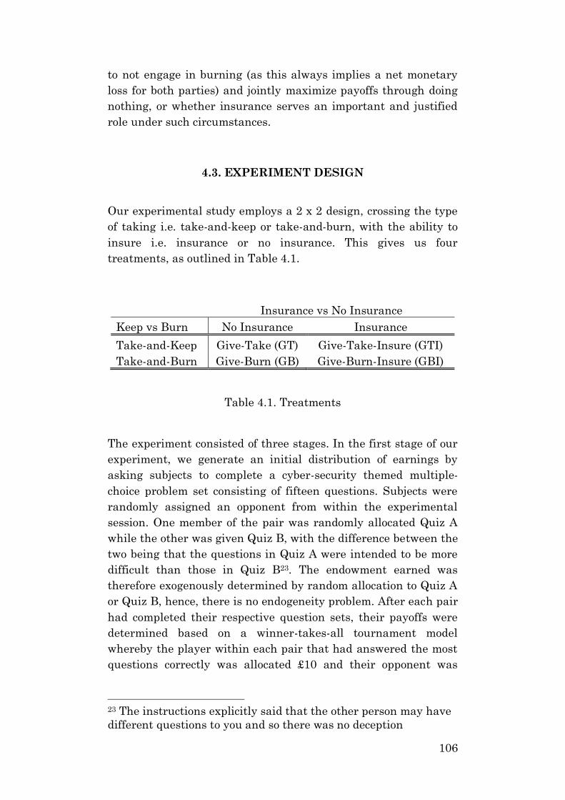
106

to not engage in burning (as this always implies a net monetary

loss for both parties) and jointly maximize payoffs through doing

nothing, or whether insurance serves an important and justified

role under such circumstances.

4.3. EXPERIMENT DESIGN

Our experimental study employs a 2 x 2 design, crossing the type

of taking i.e. take-and-keep or take-and-burn, with the ability to

insure i.e. insurance or no insurance. This gives us four

treatments, as outlined in Table 4.1.

Insurance vs No Insurance

Keep vs Burn No Insurance Insurance

Take-and-Keep Give-Take (GT) Give-Take-Insure (GTI)

Take-and-Burn Give-Burn (GB) Give-Burn-Insure (GBI)

Table 4.1. Treatments

The experiment consisted of three stages. In the first stage of our

experiment, we generate an initial distribution of earnings by

asking subjects to complete a cyber-security themed multiple-

choice problem set consisting of fifteen questions. Subjects were

randomly assigned an opponent from within the experimental

session. One member of the pair was randomly allocated Quiz A

while the other was given Quiz B, with the difference between the

two being that the questions in Quiz A were intended to be more

difficult than those in Quiz B23. The endowment earned was

therefore exogenously determined by random allocation to Quiz A

or Quiz B, hence, there is no endogeneity problem. After each pair

had completed their respective question sets, their payoffs were

determined based on a winner-takes-all tournament model

whereby the player within each pair that had answered the most

questions correctly was allocated £10 and their opponent was

23 The instructions explicitly said that the other person may have

different questions to you and so there was no deception

107

given nothing24. However, each subject was also allocated a £5

participation fee which was added to their earnings from this

round to determine the player’s endowment for the subsequent

round.

Once all participants had completed the first stage of the

experiment, we moved onto the second stage. In the second stage,

subjects were again randomly paired up with another individual

from within the experimental session and were made aware that

their opponent in the second stage differed from their opponent in

the first stage of the experiment. Each pair intentionally consisted

of one winner from the first stage, who we refer to as the “rich”

subjects or players and one loser from the first stage, who we label

as being the “poor” subjects or players. Both players were then

told the payoff they had earned from the first stage as well as the

payoff of their opponent.

It is important to note that in stage 1, subjects that were

randomly allocated the easier questions i.e. Quiz B, always won

the initial competition. As such, these subjects were always the

“rich” players in stage 2, whilst those allocated the more difficult

questions i.e. Quiz A, were invariably the “poorer” players.

Additionally, whilst subjects were told the payoff of their

opponent at the beginning of stage 2, they were not informed

about the varying levels of difficulty of to the problem sets that

both they and their opponent had completed. To be more specific,

the information set of each subject solely consisted of a) their own

payoff and b) their opponent’s payoff. That said, given the

instructions from stage 1, subjects would have also known that

the rich player was a winner in the stage 1 competition whilst the

poorer player must’ve lost against their opponent in stage 1.

Given that we are introducing a novel experiment through

incorporating a blocking or insurance strategy, our primary

objective for this particular study was to provide a simple setup in

order to test whether blocking is indeed an important component

of the give, take and do nothing mix. However, there are several

interesting future extensions of our benchmark setup. For

instance, changing the information set could provide us with

important insights. In our experiment, subjects don’t have

24 The instructions indicated that in the case of a tie one subject

would randomly be chosen to receive the £15.

108

information regarding the cause of inequality i.e. effort or luck.

With a large enough sample, one could easily adapt our design so

as to test whether providing subjects with such information at the

beginning of stage 2 has any significant effect on behaviour.

Moreover, another interesting extension would be to provide

information on the opponent’s personal characteristics, such as

social group e.g. gender or religion. This could contribute to the

literature exploring whether subjects behave differently or in a

discriminatory way when interacting with in-group versus out-

group members i.e. interaction between people within the same,

versus different, social groups25.

Subjects were subsequently asked to choose one option from the

choice-set presented to them. In the no insurance treatments,

subjects were given the option to a) take up to £2.50 from their

opponent at a cost of 10p for every 50p taken b) give up to £2.50 to

their opponent at a cost of 10p for every 50p given or c) do

nothing. In the insurance treatments, subjects had a further

choice of d) paying £1.00 to insure themselves by blocking their

opponent from being able to take their money. That is, as the

choices of subjects were not revealed to their opponents, if a

player chose to purchase insurance, any attempt to take their

money would still incur the fixed cost of taking i.e. 10p per 50p

taken, however, the subject trying to take would be blocked from

being able to access the insured player’s endowment.

Importantly, in the burning treatments, the amounts taken

(option (a)) were not transferred to or kept by the taker. Rather,

subjects were given the option to pay, under the same price

structure as in the no-burning treatments, to simply reduce, or

“burn”, up to £2.50 of their opponent’s endowment.

It is worth noting that the label of insurance on our additional

strategy is derived from the underlying motivation of our study.

However, given our design, this strategy doesn’t involve many

aspects of insurance that are found in the real-world economy,

such as risk-pooling. Therefore, although we refer to our

additional strategy as insurance throughout this chapter, one may

consider the label of blocking more accurate, as subjects are

essentially given the ability to use a prevention mechanism

25 See, for example, Chakravarty et al. (2019).

109

(perfect prevention in our case) that allows them to unilaterally

block their opponent from accessing their endowment.

To reinforce the discussion above, let 𝑒𝑖 denote the endowment of

the two subjects. Let 𝑔𝑖 and 𝑡𝑖 denote the amount subject 𝑖 gives

and takes, respectively. Finally, let 𝑠𝑖 be an indicator variable

that says whether or not subject 𝑖 paid for insurance. In the Give-

Take treatment the payoff of subject 1 matched with subject 2 (in

pounds sterling) is

𝑢𝐴 = 𝑒𝐴 − 1.2𝑔𝐴 + 𝑔𝐵 + 0.8𝑡𝐴 − 𝑡𝐵 (4.1)

In the Give-Burn treatment the payoff of subject 1 is

𝑢𝐴 = 𝑒𝐴 − 1.2𝑔𝐴 + 𝑔𝐵 − 0.2𝑡𝐴 − 𝑡𝐵 (4.2)

In the Give-Take-Insure treatment the payoff of subject 1 is

𝑢𝐴 = 𝑒𝐴 − 1.2𝑔𝐴 + 𝑔𝐵 − 0.2𝑡𝐴 + 𝑡𝐴(1 − 𝑠𝐵) − 𝑡𝐵(1 − 𝑠𝐴) − 𝑠𝐴

(4.3)

In the Give-Burn-Insure treatment the payoff of subject 1 is

𝑢𝐴 = 𝑒𝐴 − 1.2𝑔𝐴 + 𝑔𝐵 − 0.2𝑡𝐴 − 𝑡𝐵(1 − 𝑠𝐴) − 𝑠𝐴

(4.4)

It is worth noting that whilst subjects can engage in transfers so

as to equalise their payoffs in the Give-Take treatment, the richer

player will always earn more than the poorer player in the Give-

Burn treatment. Specifically, assuming that the rich player

decides to give the maximum amount of £2.50 to their poorer

opponent and that the poor player takes the maximum amount of

£2.50 from their richer counterpart, then from equation (4.1)

above, their respective payoffs in the Give-Take treatment can be

calculated as:

𝑢𝑅𝑖𝑐ℎ = 15 − 1.2(2.50) − 2.50 = 9.50

(4.5)

𝑢𝑃𝑜𝑜𝑟 = 5 + 2.50 + 0.8(2.50) = 9.50

(4.6)

Since subjects cannot take and keep money in the Give-Burn

treatment, any amount taken by the poor player would reduce

inequality by less than it would have in the Give-Take treatment.

It is clear from equation (4.2) that under the assumption that the

rich player gives £2.50 and the poor player takes £2.50 in the

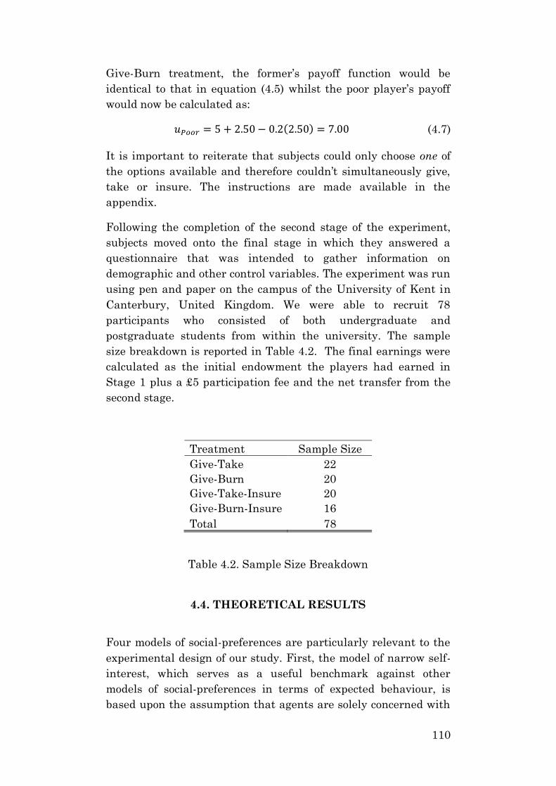
110

Give-Burn treatment, the former’s payoff function would be

identical to that in equation (4.5) whilst the poor player’s payoff

would now be calculated as:

𝑢𝑃𝑜𝑜𝑟 = 5 + 2.50 − 0.2(2.50) = 7.00

(4.7)

It is important to reiterate that subjects could only choose one of

the options available and therefore couldn’t simultaneously give,

take or insure. The instructions are made available in the

appendix.

Following the completion of the second stage of the experiment,

subjects moved onto the final stage in which they answered a

questionnaire that was intended to gather information on

demographic and other control variables. The experiment was run

using pen and paper on the campus of the University of Kent in

Canterbury, United Kingdom. We were able to recruit 78

participants who consisted of both undergraduate and

postgraduate students from within the university. The sample

size breakdown is reported in Table 4.2. The final earnings were

calculated as the initial endowment the players had earned in

Stage 1 plus a £5 participation fee and the net transfer from the

second stage.

Treatment Sample Size

Give-Take 22

Give-Burn 20

Give-Take-Insure 20

Give-Burn-Insure 16

Total 78

Table 4.2. Sample Size Breakdown

4.4. THEORETICAL RESULTS

Four models of social-preferences are particularly relevant to the

experimental design of our study. First, the model of narrow self-

interest, which serves as a useful benchmark against other

models of social-preferences in terms of expected behaviour, is

based upon the assumption that agents are solely concerned with

111

the maximization of their personal monetary payoffs. In

accordance with this model, the preferences of agents can be

represented by the following straightforward utility function:

𝑈𝐴 = 𝑢𝐴

(4.8)

Where 𝑢𝐴 indicates the monetary payoff of the agent. As

described, the utility of agents is increasing in only their own

monetary payoff. In other words, the higher an individual’s

monetary payoff, the higher is their utility.

While the model of narrow self-interest is commonly applied

throughout the economic literature, numerous studies have found

the assumption of agents being entirely self-regarding to be overly

simplistic and inaccurate across a multiplicity of contexts. As

mentioned earlier, prior literature has provided strong evidence

for the existence of so-called other regarding preferences. The

seminal model of inequality aversion (Fehr and Schmidt 1999)

provides an extension to the model of narrow self-interest by

postulating that individuals are not only positively concerned

about their own monetary payoffs but are also negatively affected

by the difference between their own payoff and that of the other.

Therefore, if agents display inequality aversion i.e. they dislike

inequality, then they may be willing to sacrifice a percentage of

their own wealth or endowment for the purpose of reaching a

more egalitarian distribution of outcomes through reallocation.

Under a simple two-person setting, the utility function of agents

within the model of inequality-aversion can be written as:

𝑈𝐴(𝑢𝐴, 𝑢𝐵) = 𝑢𝐴 − 𝑎𝐴 max{𝑢𝐵 − 𝑢𝐴, 0} − 𝛽𝐴𝑚𝑎𝑥{𝑢𝐴 − 𝑢𝐵 , 0}

(4.9)

Where 𝑢𝐴 indicates the monetary payoff to Person A and 𝑢𝐵

denotes the payoff to Person B. The second term on the right hand

side of the equation measures the loss of utility from

disadvantageous inequality. The larger the parameter 𝑎𝐴, which

is sometimes referred to as a measure of envy, the more Person A

dislikes disadvantageous inequality. Similarly, the third term

measures the loss of utility from advantageous inequality. The

larger the parameter 𝛽𝐴, also described as a parameter measuring

the degree of guilt, the more Person A dislikes advantageous

inequality. In their original study, Fehr and Schmidt (1999)

assume that 0 ≤ 𝛽 < 1, which not only implies that agents do not

enjoy advantageous inequality but that they also wouldn’t be

112

willing to burn their own money to mitigate an advantageous

position. An additional assumption made by Fehr and Schmidt

(1999) is that 𝑎𝐴 ≥ 𝛽𝐴. In other words, individuals dislike

disadvantageous inequality i.e. being poorer than the other, more

than they dislike advantageous inequality i.e. being richer than

the other.

While the assumption that agents hold a greater aversion towards

disadvantageous inequality in comparison to advantageous

inequality has a strong intuitive appeal and is also supported by

prior findings in social psychology (Messick and Sentis (1985) and

Loewenstein et al. (1989)), more recent studies have found this

assumption to be regularly violated empirically (Dannenberg et

al. (2007), Bellemare et al. (2008), Blanco et al. (2011) and Yang

et al. (2016)).

A further important form of other-regarding preferences that has

received widespread empirical support is that of altruism. The

model of altruism posits that agents are not only concerned about

their own wealth or payoffs but that they also care positively

about the payoff of others. In this study, we consider a model of

altruism based upon a restricted version of the Fehr and Schmidt

(1999) model presented above. Under the simple two-individual

setting in this model, the utility function of agents is written as:

𝑈𝐴(𝑢𝐴, 𝑢𝐵) = 𝑢𝐴 − 𝜃𝐴𝑚𝑎𝑥{𝑢𝐴 − 𝑢𝐵 , 0}

(4.10)

Where the parameter 𝜃 measures, and is increasing in, the degree

of altruism. It is assumed that 0 < 𝜃𝐴 ≤ 1. Hence, the larger the

parameter of altruism the more the subject cares about the

monetary payoff of the other. If 𝜃 = 1 then the subject cares about

the monetary payoff of the other as much their own payoff. As

shown in (4.10), the utility of agents is decreasing in the amount

of advantageous inequality whilst being unaffected by

disadvantageous inequality, which differentiates this model of

altruism from the model of inequality-aversion described above.

That is, if Person A is richer than Person B, then the second term

on the right hand side of equation (4.10) is positive. In contrast, if

Person A is poorer than Person B, this term then becomes

irrelevant.

113

The final model of social-preferences we take into consideration is

that of spite (or envy)26. This model assumes that an agent’s

utility is a positive function of their personal monetary payoff but,

as spiteful or envious agents dislike being worse off than others,

their utility is decreasing in the size of any disadvantageous

inequality. Similar to the model of altruism presented above, the

model of envy constitutes a restricted form of the Fehr and

Schmidt (1999) model of inequality-aversion. In the two-person

case, the utility function of agents is expressed as:

𝑈𝐴(𝑢𝐴, 𝑢𝐵) = 𝑢𝐴 − 𝐴𝑚𝑎𝑥{𝑢𝐵 − 𝑢𝐴, 0}

(4.11)

Where the parameter 0 < ≤ 1 provides a measure of the degree

of envy. If = 1, the subject cares about disadvantageous

inequality as much as their own monetary payoff. As described,

an envious agent’s utility is decreasing in both the degree of envy

and the extent of disadvantageous inequality. If the subject has a

higher payoff than their opponent i.e. 𝑢𝐵 − 𝑢𝐴 < 0, then the second

term on the right hand side of the equation becomes irrelevant

and the utility function becomes identical to that in the model of

narrow self-interest as in (4.8).

4.4.1. Theoretical Results for Self-Motivated

We take it as given that there will be heterogeneity across the

population in terms of social-preferences. Therefore, some people

behave as if maximising their personal monetary payoff, others

inequality averse and so on. In the following, we derive results

regarding the possible behaviour of subjects in our experiment

based on the four models of social-preferences. These results are

also summarised in Table 4.3. We begin with a result that

requires no proof.

Proposition 1: An individual who is concerned with maximizing

their personal monetary payoff should take the maximum £2.50

in the Give-Take treatment and do nothing in the Give-Burn

treatment.

You can see that in the treatments without insurance, the optimal

behaviour of a selfish individual does not depend on the behaviour

of their opponent. Once we add insurance this changes. Now

26 Note that for the purposes of this study we use the terms spite

and envy interchangeably.

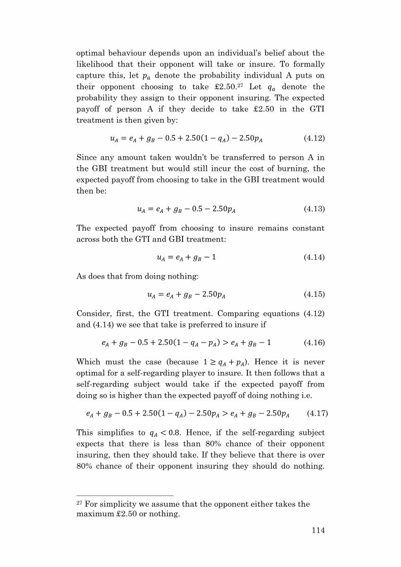
114

optimal behaviour depends upon an individual’s belief about the

likelihood that their opponent will take or insure. To formally

capture this, let 𝑝𝑎 denote the probability individual A puts on

their opponent choosing to take £2.50.27 Let 𝑞𝑎 denote the

probability they assign to their opponent insuring. The expected

payoff of person A if they decide to take £2.50 in the GTI

treatment is then given by:

𝑢𝐴 = 𝑒𝐴 + 𝑔𝐵 − 0.5 + 2.50(1 − 𝑞𝐴) − 2.50𝑝𝐴

(4.12)

Since any amount taken wouldn’t be transferred to person A in

the GBI treatment but would still incur the cost of burning, the

expected payoff from choosing to take in the GBI treatment would

then be:

𝑢𝐴 = 𝑒𝐴 + 𝑔𝐵 − 0.5 − 2.50𝑝𝐴

(4.13)

The expected payoff from choosing to insure remains constant

across both the GTI and GBI treatment:

𝑢𝐴 = 𝑒𝐴 + 𝑔𝐵 − 1

(4.14)

As does that from doing nothing:

𝑢𝐴 = 𝑒𝐴 + 𝑔𝐵 − 2.50𝑝𝐴

(4.15)

Consider, first, the GTI treatment. Comparing equations (4.12)

and (4.14) we see that take is preferred to insure if

𝑒𝐴 + 𝑔𝐵 − 0.5 + 2.50(1 − 𝑞𝐴 − 𝑝𝐴) > 𝑒𝐴 + 𝑔𝐵 − 1

(4.16)

Which must the case (because 1 ≥ 𝑞𝐴 + 𝑝𝐴). Hence it is never

optimal for a self-regarding player to insure. It then follows that a

self-regarding subject would take if the expected payoff from

doing so is higher than the expected payoff of doing nothing i.e.

𝑒𝐴 + 𝑔𝐵 − 0.5 + 2.50(1 − 𝑞𝐴) − 2.50𝑝𝐴 > 𝑒𝐴 + 𝑔𝐵 − 2.50𝑝𝐴

(4.17)

This simplifies to 𝑞𝐴 < 0.8. Hence, if the self-regarding subject

expects that there is less than 80% chance of their opponent

insuring, then they should take. If they believe that there is over

80% chance of their opponent insuring they should do nothing.

27 For simplicity we assume that the opponent either takes the

maximum £2.50 or nothing.

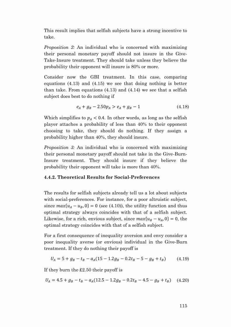
115

This result implies that selfish subjects have a strong incentive to

take.


their personal monetary payoff should not insure in the Give-

Take-Insure treatment. They should take unless they believe the

probability their opponent will insure is 80% or more.

Consider now the GBI treatment. In this case, comparing

equations (4.13) and (4.15) we see that doing nothing is better

than take. From equations (4.13) and (4.14) we see that a selfish

subject does best to do nothing if

𝑒𝐴 + 𝑔𝐵 − 2.50𝑝𝐴 > 𝑒𝐴 + 𝑔𝐵 − 1

(4.18)

Which simplifies to 𝑝𝐴 < 0.4. In other words, as long as the selfish

player attaches a probability of less than 40% to their opponent

choosing to take, they should do nothing. If they assign a

probability higher than 40%, they should insure.


their personal monetary payoff should not take in the Give-Burn-

Insure treatment. They should insure if they believe the

probability their opponent will take is more than 40%.

4.4.2. Theoretical Results for Social-Preferences

The results for selfish subjects already tell us a lot about subjects

with social-preferences. For instance, for a poor altruistic subject,

since 𝑚𝑎𝑥{𝑢𝐴 − 𝑢𝐵 , 0} = 0 (see (4.10)), the utility function and thus

optimal strategy always coincides with that of a selfish subject.

Likewise, for a rich, envious subject, since 𝑚𝑎𝑥{𝑢𝐵 − 𝑢𝐴, 0} = 0, the

optimal strategy coincides with that of a selfish subject.

For a first consequence of inequality aversion and envy consider a

poor inequality averse (or envious) individual in the Give-Burn

treatment. If they do nothing their payoff is

𝑈𝐴 = 5 + 𝑔𝐵 − 𝑡𝐵 − 𝑎𝐴(15 − 1.2𝑔𝐵 − 0.2𝑡𝐵 − 5 − 𝑔𝐵 + 𝑡𝐵)

(4.19)

If they burn the £2.50 their payoff is

𝑈𝐴 = 4.5 + 𝑔𝐵 − 𝑡𝐵 − 𝑎𝐴(12.5 − 1.2𝑔𝐵 − 0.2𝑡𝐵 − 4.5 − 𝑔𝐵 + 𝑡𝐵)

(4.20)

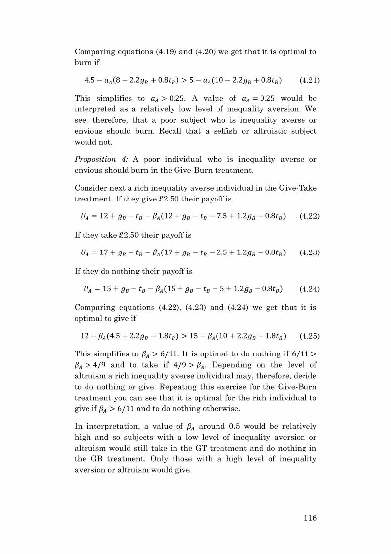
116

Comparing equations (4.19) and (4.20) we get that it is optimal to

burn if

4.5 − 𝑎𝐴(8 − 2.2𝑔𝐵 + 0.8𝑡𝐵) > 5 − 𝑎𝐴(10 − 2.2𝑔𝐵 + 0.8𝑡𝐵) (4.21)

This simplifies to 𝑎𝐴 > 0.25. A value of 𝑎𝐴 = 0.25 would be

interpreted as a relatively low level of inequality aversion. We

see, therefore, that a poor subject who is inequality averse or

envious should burn. Recall that a selfish or altruistic subject

would not.

Proposition 4: A poor individual who is inequality averse or

envious should burn in the Give-Burn treatment.

Consider next a rich inequality averse individual in the Give-Take

treatment. If they give £2.50 their payoff is

𝑈𝐴 = 12 + 𝑔𝐵 − 𝑡𝐵 − 𝛽𝐴(12 + 𝑔𝐵 − 𝑡𝐵 − 7.5 + 1.2𝑔𝐵 − 0.8𝑡𝐵)

(4.22)

If they take £2.50 their payoff is

𝑈𝐴 = 17 + 𝑔𝐵 − 𝑡𝐵 − 𝛽𝐴(17 + 𝑔𝐵 − 𝑡𝐵 − 2.5 + 1.2𝑔𝐵 − 0.8𝑡𝐵)

(4.23)

If they do nothing their payoff is

𝑈𝐴 = 15 + 𝑔𝐵 − 𝑡𝐵 − 𝛽𝐴(15 + 𝑔𝐵 − 𝑡𝐵 − 5 + 1.2𝑔𝐵 − 0.8𝑡𝐵)

(4.24)

Comparing equations (4.22), (4.23) and (4.24) we get that it is

optimal to give if

12 − 𝛽𝐴(4.5 + 2.2𝑔𝐵 − 1.8𝑡𝐵) > 15 − 𝛽𝐴(10 + 2.2𝑔𝐵 − 1.8𝑡𝐵) (4.25)

This simplifies to 𝛽𝐴 > 6/11. It is optimal to do nothing if 6/11 >

𝛽𝐴 > 4/9 and to take if 4/9 > 𝛽𝐴. Depending on the level of

altruism a rich inequality averse individual may, therefore, decide

to do nothing or give. Repeating this exercise for the Give-Burn

treatment you can see that it is optimal for the rich individual to

give if 𝛽𝐴 > 6/11 and to do nothing otherwise.

In interpretation, a value of 𝛽𝐴 around 0.5 would be relatively

high and so subjects with a low level of inequality aversion or

altruism would still take in the GT treatment and do nothing in

the GB treatment. Only those with a high level of inequality

aversion or altruism would give.

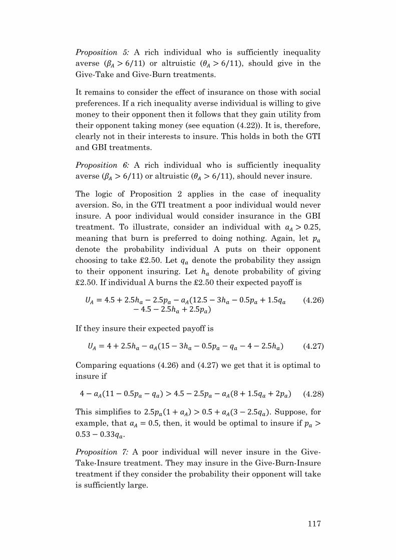
117

Proposition 5: A rich individual who is sufficiently inequality

averse (𝛽𝐴 > 6/11) or altruistic (𝜃𝐴 > 6/11), should give in the

Give-Take and Give-Burn treatments.

It remains to consider the effect of insurance on those with social

preferences. If a rich inequality averse individual is willing to give

money to their opponent then it follows that they gain utility from

their opponent taking money (see equation (4.22)). It is, therefore,

clearly not in their interests to insure. This holds in both the GTI

and GBI treatments.

Proposition 6: A rich individual who is sufficiently inequality

averse (𝛽𝐴 > 6/11) or altruistic (𝜃𝐴 > 6/11), should never insure.

The logic of Proposition 2 applies in the case of inequality

aversion. So, in the GTI treatment a poor individual would never

insure. A poor individual would consider insurance in the GBI

treatment. To illustrate, consider an individual with 𝑎𝐴 > 0.25,

meaning that burn is preferred to doing nothing. Again, let 𝑝𝑎

denote the probability individual A puts on their opponent

choosing to take £2.50. Let 𝑞𝑎 denote the probability they assign

to their opponent insuring. Let ℎ𝑎 denote probability of giving

£2.50. If individual A burns the £2.50 their expected payoff is

𝑈𝐴 = 4.5 + 2.5ℎ𝑎 − 2.5𝑝𝑎 − 𝑎𝐴(12.5 − 3ℎ𝑎 − 0.5𝑝𝑎 + 1.5𝑞𝑎

− 4.5 − 2.5ℎ𝑎 + 2.5𝑝𝑎)

(4.26)

If they insure their expected payoff is

𝑈𝐴 = 4 + 2.5ℎ𝑎 − 𝑎𝐴(15 − 3ℎ𝑎 − 0.5𝑝𝑎 − 𝑞𝑎 − 4 − 2.5ℎ𝑎)

(4.27)

Comparing equations (4.26) and (4.27) we get that it is optimal to

insure if

4 − 𝑎𝐴(11 − 0.5𝑝𝑎 − 𝑞𝑎) > 4.5 − 2.5𝑝𝑎 − 𝑎𝐴(8 + 1.5𝑞𝑎 + 2𝑝𝑎) (4.28)

This simplifies to 2.5𝑝𝑎(1 + 𝑎𝐴) > 0.5 + 𝑎𝐴(3 − 2.5𝑞𝑎). Suppose, for

example, that 𝑎𝐴 = 0.5, then, it would be optimal to insure if 𝑝𝑎 >

0.53 − 0.33𝑞𝑎.

Proposition 7: A poor individual will never insure in the Give-

Take-Insure treatment. They may insure in the Give-Burn-Insure

treatment if they consider the probability their opponent will take

is sufficiently large.

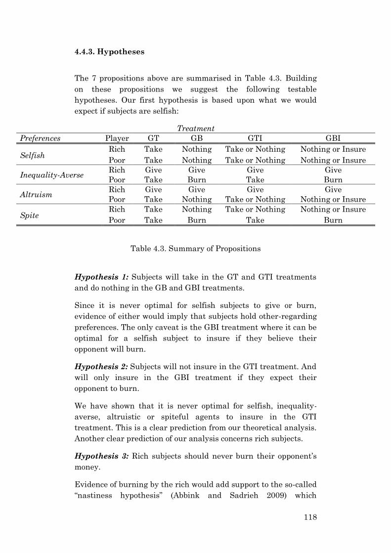
118

4.4.3. Hypotheses

The 7 propositions above are summarised in Table 4.3. Building

on these propositions we suggest the following testable

hypotheses. Our first hypothesis is based upon what we would

expect if subjects are selfish:

Treatment

Preferences Player GT GB GTI GBI

Selfish Rich Take Nothing Take or Nothing Nothing or Insure

Poor Take Nothing Take or Nothing Nothing or Insure

Inequality-Averse Rich Give Give Give Give

Poor Take Burn Take Burn

Altruism Rich Give Give Give Give

Poor Take Nothing Take or Nothing Nothing or Insure

Spite Rich Take Nothing Take or Nothing Nothing or Insure

Poor Take Burn Take Burn

Table 4.3. Summary of Propositions

Hypothesis 1: Subjects will take in the GT and GTI treatments

and do nothing in the GB and GBI treatments.

Since it is never optimal for selfish subjects to give or burn,

evidence of either would imply that subjects hold other-regarding

preferences. The only caveat is the GBI treatment where it can be

optimal for a selfish subject to insure if they believe their

opponent will burn.

Hypothesis 2: Subjects will not insure in the GTI treatment. And

will only insure in the GBI treatment if they expect their

opponent to burn.

We have shown that it is never optimal for selfish, inequality-

averse, altruistic or spiteful agents to insure in the GTI

treatment. This is a clear prediction from our theoretical analysis.

Another clear prediction of our analysis concerns rich subjects.

Hypothesis 3: Rich subjects should never burn their opponent’s

money.

Evidence of burning by the rich would add support to the so-called

“nastiness hypothesis” (Abbink and Sadrieh 2009) which

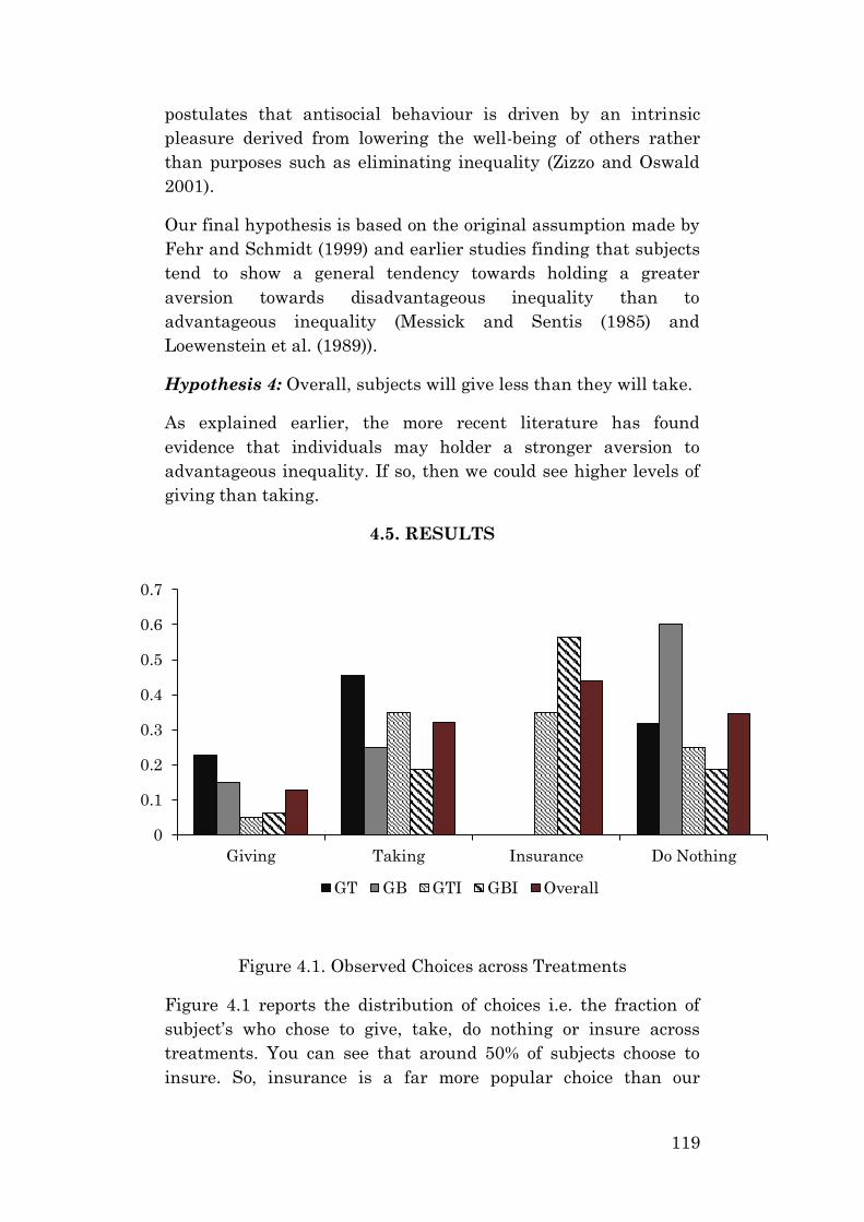
119

postulates that antisocial behaviour is driven by an intrinsic

pleasure derived from lowering the well-being of others rather

than purposes such as eliminating inequality (Zizzo and Oswald

2001).

Our final hypothesis is based on the original assumption made by

Fehr and Schmidt (1999) and earlier studies finding that subjects

tend to show a general tendency towards holding a greater

aversion towards disadvantageous inequality than to

advantageous inequality (Messick and Sentis (1985) and

Loewenstein et al. (1989)).

Hypothesis 4: Overall, subjects will give less than they will take.

As explained earlier, the more recent literature has found

evidence that individuals may holder a stronger aversion to

advantageous inequality. If so, then we could see higher levels of

giving than taking.

4.5. RESULTS

Figure 4.1. Observed Choices across Treatments

Figure 4.1 reports the distribution of choices i.e. the fraction of

subject’s who chose to give, take, do nothing or insure across

treatments. You can see that around 50% of subjects choose to

insure. So, insurance is a far more popular choice than our

0

0.1

0.2

0.3

0.4

0.5

0.6

0.7

Giving Taking Insurance Do Nothing

GT GB GTI GBI Overall

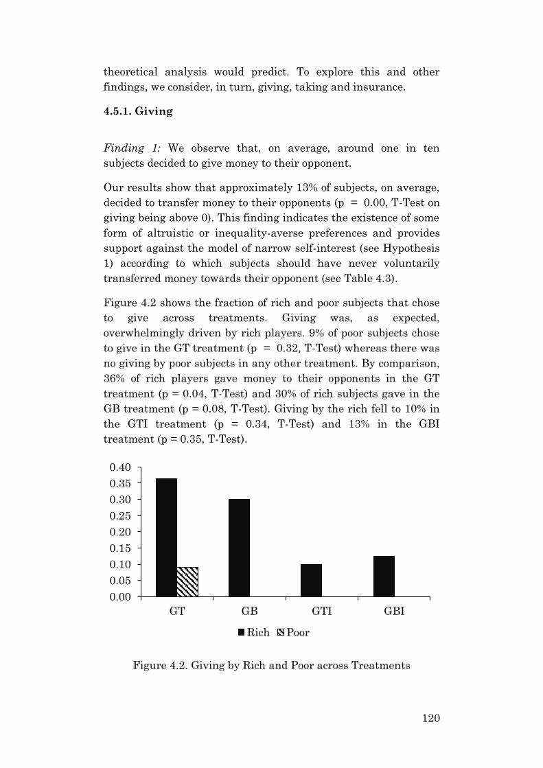
120

theoretical analysis would predict. To explore this and other

findings, we consider, in turn, giving, taking and insurance.

4.5.1. Giving

Finding 1: We observe that, on average, around one in ten

subjects decided to give money to their opponent.

Our results show that approximately 13% of subjects, on average,

decided to transfer money to their opponents (p = 0.00, T-Test on

giving being above 0). This finding indicates the existence of some

form of altruistic or inequality-averse preferences and provides

support against the model of narrow self-interest (see Hypothesis

1) according to which subjects should have never voluntarily

transferred money towards their opponent (see Table 4.3).

Figure 4.2 shows the fraction of rich and poor subjects that chose

to give across treatments. Giving was, as expected,

overwhelmingly driven by rich players. 9% of poor subjects chose

to give in the GT treatment (p = 0.32, T-Test) whereas there was

no giving by poor subjects in any other treatment. By comparison,

36% of rich players gave money to their opponents in the GT

treatment (p = 0.04, T-Test) and 30% of rich subjects gave in the

GB treatment (p = 0.08, T-Test). Giving by the rich fell to 10% in

the GTI treatment (p = 0.34, T-Test) and 13% in the GBI

treatment (p = 0.35, T-Test).

Figure 4.2. Giving by Rich and Poor across Treatments

0.00

0.05

0.10

0.15

0.20

0.25

0.30

0.35

0.40

GT GB GTI GBI

Rich Poor

121

Finding 2: Extending the choice-set to include the option to insure

lowers giving.

The fraction of subjects that decided to give money to their

opponents fell from 23% in the GT treatment to 5% in the GTI

treatment (giving in the GT versus GTI treatment, p = 0.10

Proportions Test, p = 0.08 T-Test) and from 15% in the GB

treatment to 6.25% in the GBI treatment (p = 0.41 Proportions

Test, p = 0.38 T-Test). If we compare the proportion of subjects

willing to give in the no insurance treatment i.e. GT plus GB with

the proportion of subjects willing to give in the insurance

treatment i.e. GTI plus GBI, we find that extending the choice-set

to include the option to insure significantly lowers the fraction of

subject’s willing to give from 19% to 6% (p = 0.08 Proportions

Test, p = 0.06 T-Test). Our results show a marginally significant

reduction in the fraction of rich subjects willing to give from 33%

in the no insurance treatment to 11% in the insurance treatment

(p = 0.10 Proportions Test, 0.07 T-Test).

Our theoretical analysis suggested that the introduction of an

insurance option, ceteris paribus, shouldn’t influence subjects’

willingness to give. Basically, if a subject is willing to give then

they should also be willing to let their opponent take. The

apparent reversal in generosity observed in our experiment is

consistent with the so-called contextual preference reversal and

reference dependence of preferences (see Easterlin (1995), Clark

and Oswald (1996), Kahneman et al. (2000), Laynard (2003), List

(2007) and Bardsley (2008)). In particular, the choice set may

have served as an indicator of appropriate behaviour and social

norms. For instance, the option of insurance may have led to

subjects to put more weight on their opponent taking, which then

crowds out a desire to give.

Finding 3: There is no statistically significant difference in giving

between the taking and burning treatments.

Overall, we find that 11% of subjects gave in the burn treatment

whereas 14% of subjects chose to give in the taking treatment

(giving in the taking versus burn treatment, p = 0.68 Proportions

Test, p = 0.11 T-Test). Similarly, 24% of rich subjects chose to

give in the take-and-keep treatment whereas 22% gave in the

burn treatment (p = 0.91 Proportions Test, p = 0.91 T-Test).

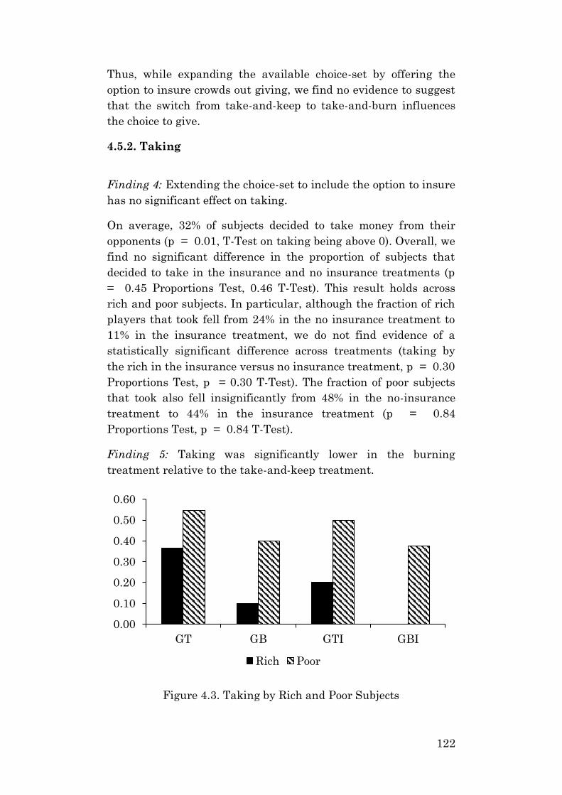
122

Thus, while expanding the available choice-set by offering the

option to insure crowds out giving, we find no evidence to suggest

that the switch from take-and-keep to take-and-burn influences

the choice to give.

4.5.2. Taking

Finding 4: Extending the choice-set to include the option to insure

has no significant effect on taking.

On average, 32% of subjects decided to take money from their

opponents (p = 0.01, T-Test on taking being above 0). Overall, we

find no significant difference in the proportion of subjects that

decided to take in the insurance and no insurance treatments (p

= 0.45 Proportions Test, 0.46 T-Test). This result holds across

rich and poor subjects. In particular, although the fraction of rich

players that took fell from 24% in the no insurance treatment to

11% in the insurance treatment, we do not find evidence of a

statistically significant difference across treatments (taking by

the rich in the insurance versus no insurance treatment, p = 0.30

Proportions Test, p = 0.30 T-Test). The fraction of poor subjects

that took also fell insignificantly from 48% in the no-insurance

treatment to 44% in the insurance treatment (p = 0.84

Proportions Test, p = 0.84 T-Test).

Finding 5: Taking was significantly lower in the burning

treatment relative to the take-and-keep treatment.

Figure 4.3. Taking by Rich and Poor Subjects

0.00

0.10

0.20

0.30

0.40

0.50

0.60

GT GB GTI GBI

Rich Poor

123

We find evidence of a reduction in the fraction of subjects that

decided to take from 40% in the taking treatment to 22% in the

burning treatment (taking in the taking versus burn treatment, p

= 0.09 Proportions Test, p = 0.07 T-Test). Interestingly, this

result doesn’t hold when we compare the behaviour of rich and

poor players. In particular, as shown in Figure 4.3, we find that

the fraction of rich subjects that took fell from 29% in the taking

treatment to 6% in the burning treatment (p = 0.06 Proportions

Test, p = 0.05 T-Test) while the fraction of poor subjects that

took fell insignificantly from 52% in the taking treatment to 39%

in the burning treatment (p = 0.40 Proportions-Test, p = 0.40 T-

Test). Moreover, while taking by the poor is individually

significant in every treatment (p = 0.01 (GT), p = 0.04 (GB), p =

0.02 (GTI), p = 0.08 (GBI)), our results suggest that taking by

the rich is only significant in the GT treatment (p = 0.04).

Our finding of there being no statistical difference in the fraction

of poor subjects that took across the taking and burning

treatments lends support to the notion that burning is primarily

driven out of an aversion towards disadvantageous inequality

(Zizzo and Oswald 2001) rather than pure nastiness (Abbink and

Sadrieh 2009). That is, the absence of any significant burning by

rich subjects implies that we do not find evidence in support of the

so-called nastiness hypothesis which postulates that observed

antisocial behaviour is triggered by an intrinsic pleasure derived

from lowering the well-being of others. Rather, the decrease in the

fraction of rich subjects that took in the burn treatment relative to

the take-and-keep treatment suggests that taking by the rich was

primarily motivated by self-interest rather than pure nastiness,

which adds support towards Hypothesis 3.

The fact that we do not observe any significant difference in

taking across the take-and-keep and burn treatments among poor

subjects raises an interesting question regarding the external

validity and thus real-world implications of our findings. That is,

we show that in a lab setting, subjects were willing to incur a net

personal cost in order to counter disadvantageous inequality. This

finding is in line with a number of studies that have shown that

individuals derive utility from relative status (Frank (1985),

Robson (1992), Solnick and Hemenway (2007) and Grolleau and

Said (2009)), that they dislike being of a lower rank than others

124

(Bault et al. (2008) and Ferrer-i-Carbonnel (2005)) and that they

are willing to invest resources to prevent themselves from being

beneath others (Beckman et al. (2002) and Zizzo and Oswald

(2001)).

However, while taking money in the take-and-keep treatment

involved a reallocation of wealth and possible net advantage in

monetary terms for the taker, evidence of burning implies that

agents were willing to waste resources and lower the level of

tangible welfare in order to improve their relative position in the

income hierarchy. At a more practical level, there are numerous

documented accounts of hostility towards individuals that are

more successful than the perpetrators (Smith 1990, Mui 1995 and

Fehr 2015).

Several authors have argued that such sabotaging behaviour

targeted at better-off individuals can discourage

entrepreneurship, innovation, economic growth and development

(Schoeck (1966), Mui (1995), Caplan et al. (2005) and Fehr

(2018)). The ramifications of such behaviour are therefore likely to

have a negative feedback effect on saboteurs in the longer-run. In

combination with the common finding within the empirical

literature showing that poorer households tend to depict a higher

degree of impatience in terms of their time-preferences (see

Carvalho 2010), if poorer agents don’t place a high enough weight

on future prospects, then this result may further suggest that

poorer agents are more willing to directly inflict punishment upon

others and inadvertently promote self-sabotage in the longer-term

as a consequence.

Moreover, this result could also be relevant for discussions on

organizational settings. For instance, several organizations

commonly implement tournament or competition-type

compensation schemes whereby earnings and promotions are

dependent upon relative performance comparisons (Bognanno

2001, Bothner, Kang and Stuart 2007 and Casas-Arce and

Martinez-Jerez 2009). However, in combination with earlier

studies, our results suggest that such setups could elicit negative

emotions and interactions which may ultimately hamper

cooperation between agents.

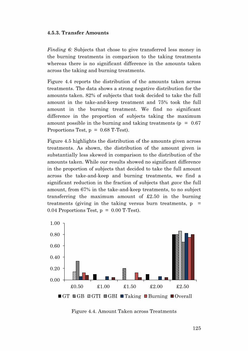
125

4.5.3. Transfer Amounts

Finding 6: Subjects that chose to give transferred less money in

the burning treatments in comparison to the taking treatments

whereas there is no significant difference in the amounts taken

across the taking and burning treatments.

Figure 4.4 reports the distribution of the amounts taken across

treatments. The data shows a strong negative distribution for the

amounts taken. 82% of subjects that took decided to take the full

amount in the take-and-keep treatment and 75% took the full

amount in the burning treatment. We find no significant

difference in the proportion of subjects taking the maximum

amount possible in the burning and taking treatments (p = 0.67


Figure 4.5 highlights the distribution of the amounts given across

treatments. As shown, the distribution of the amount given is

substantially less skewed in comparison to the distribution of the

amounts taken. While our results showed no significant difference

in the proportion of subjects that decided to take the full amount

across the take-and-keep and burning treatments, we find a

significant reduction in the fraction of subjects that gave the full

amount, from 67% in the take-and-keep treatments, to no subject

transferring the maximum amount of £2.50 in the burning

treatments (giving in the taking versus burn treatments, p =

0.04 Proportions Test, p = 0.00 T-Test).

Figure 4.4. Amount Taken across Treatments

0.00

0.20

0.40

0.60

0.80

1.00

£0.50 £1.00 £1.50 £2.00 £2.50

GT GB GTI GBI Taking Burning Overall

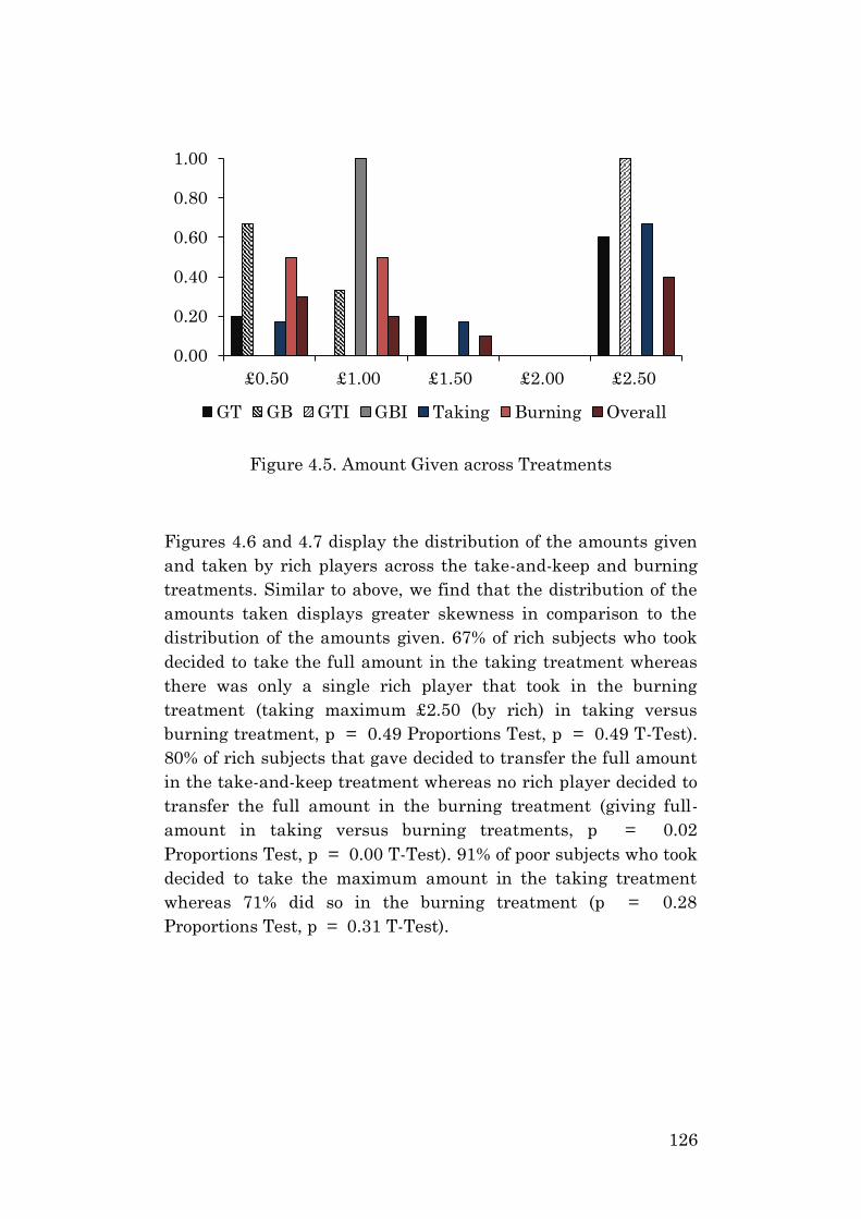
126

Figure 4.5. Amount Given across Treatments

Figures 4.6 and 4.7 display the distribution of the amounts given

and taken by rich players across the take-and-keep and burning

treatments. Similar to above, we find that the distribution of the

amounts taken displays greater skewness in comparison to the

distribution of the amounts given. 67% of rich subjects who took

decided to take the full amount in the taking treatment whereas

there was only a single rich player that took in the burning

treatment (taking maximum £2.50 (by rich) in taking versus

burning treatment, p = 0.49 Proportions Test, p = 0.49 T-Test).

80% of rich subjects that gave decided to transfer the full amount

in the take-and-keep treatment whereas no rich player decided to

transfer the full amount in the burning treatment (giving full-

amount in taking versus burning treatments, p = 0.02

Proportions Test, p = 0.00 T-Test). 91% of poor subjects who took

decided to take the maximum amount in the taking treatment

whereas 71% did so in the burning treatment (p = 0.28


0.00

0.20

0.40

0.60

0.80

1.00

£0.50 £1.00 £1.50 £2.00 £2.50

GT GB GTI GBI Taking Burning Overall

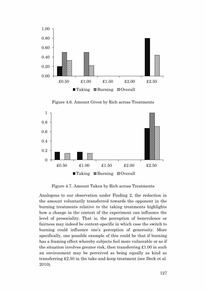
127

Figure 4.6. Amount Given by Rich across Treatments

Figure 4.7. Amount Taken by Rich across Treatments

Analogous to our observation under Finding 2, the reduction in

the amount voluntarily transferred towards the opponent in the

burning treatments relative to the taking treatments highlights

how a change in the context of the experiment can influence the

level of prosociality. That is, the perception of benevolence or

fairness may indeed be context-specific in which case the switch to

burning could influence one’s perception of generosity. More

specifically, one possible example of this could be that if burning

has a framing effect whereby subjects feel more vulnerable or as if

the situation involves greater risk, then transferring £1.00 in such

an environment may be perceived as being equally as kind as

transferring £2.50 in the take-and-keep treatment (see Deck et al.

2010).

0.00

0.20

0.40

0.60

0.80

1.00

£0.50 £1.00 £1.50 £2.00 £2.50

Taking Burning Overall

0

0.2

0.4

0.6

0.8

1

£0.50 £1.00 £1.50 £2.00 £2.50

Taking Burning Overall

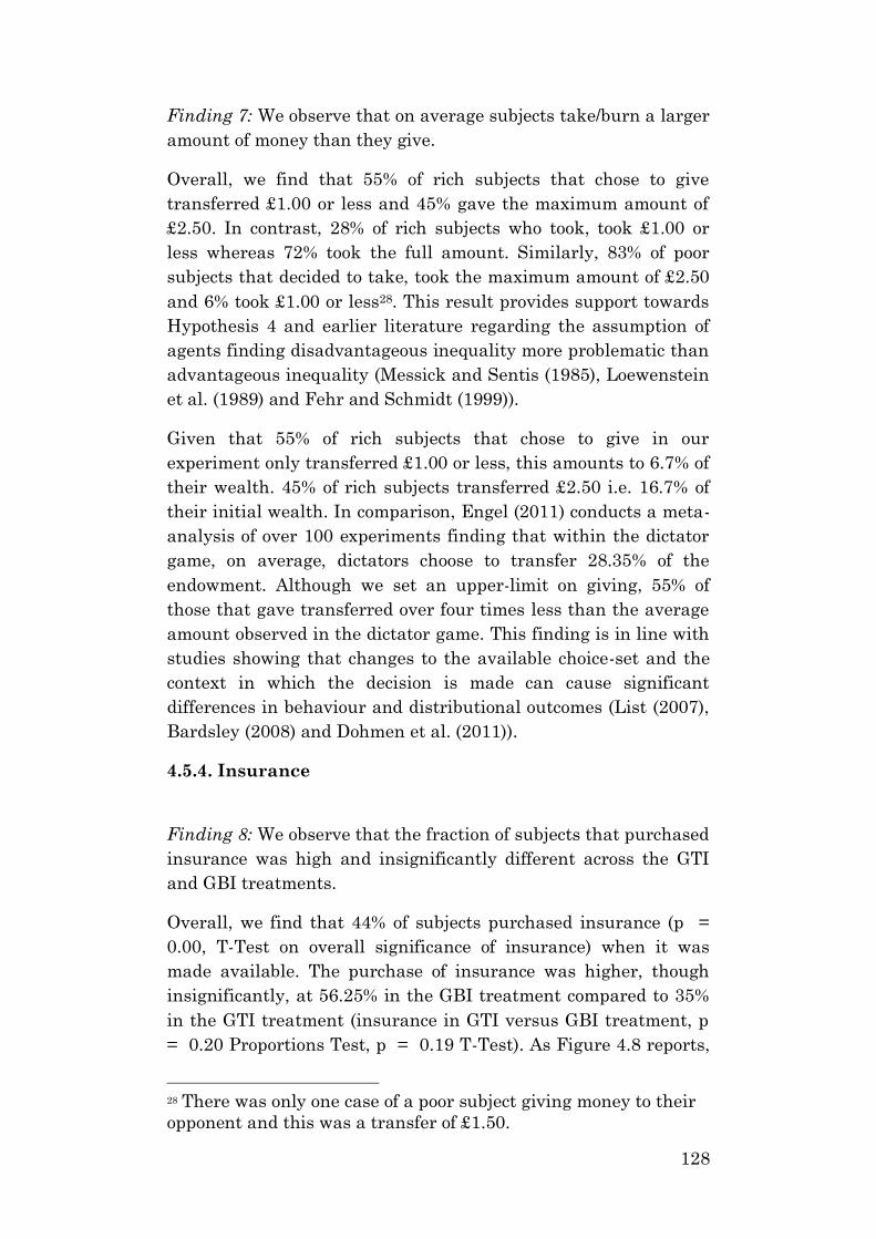
128

Finding 7: We observe that on average subjects take/burn a larger

amount of money than they give.

Overall, we find that 55% of rich subjects that chose to give

transferred £1.00 or less and 45% gave the maximum amount of

£2.50. In contrast, 28% of rich subjects who took, took £1.00 or

less whereas 72% took the full amount. Similarly, 83% of poor

subjects that decided to take, took the maximum amount of £2.50

and 6% took £1.00 or less28. This result provides support towards

Hypothesis 4 and earlier literature regarding the assumption of

agents finding disadvantageous inequality more problematic than

advantageous inequality (Messick and Sentis (1985), Loewenstein

et al. (1989) and Fehr and Schmidt (1999)).

Given that 55% of rich subjects that chose to give in our

experiment only transferred £1.00 or less, this amounts to 6.7% of

their wealth. 45% of rich subjects transferred £2.50 i.e. 16.7% of

their initial wealth. In comparison, Engel (2011) conducts a meta-

analysis of over 100 experiments finding that within the dictator

game, on average, dictators choose to transfer 28.35% of the

endowment. Although we set an upper-limit on giving, 55% of

those that gave transferred over four times less than the average

amount observed in the dictator game. This finding is in line with

studies showing that changes to the available choice-set and the

context in which the decision is made can cause significant

differences in behaviour and distributional outcomes (List (2007),

Bardsley (2008) and Dohmen et al. (2011)).

4.5.4. Insurance

Finding 8: We observe that the fraction of subjects that purchased

insurance was high and insignificantly different across the GTI

and GBI treatments.

Overall, we find that 44% of subjects purchased insurance (p =

0.00, T-Test on overall significance of insurance) when it was

made available. The purchase of insurance was higher, though

insignificantly, at 56.25% in the GBI treatment compared to 35%

in the GTI treatment (insurance in GTI versus GBI treatment, p

= 0.20 Proportions Test, p = 0.19 T-Test). As Figure 4.8 reports,

28 There was only one case of a poor subject giving money to their

opponent and this was a transfer of £1.50.

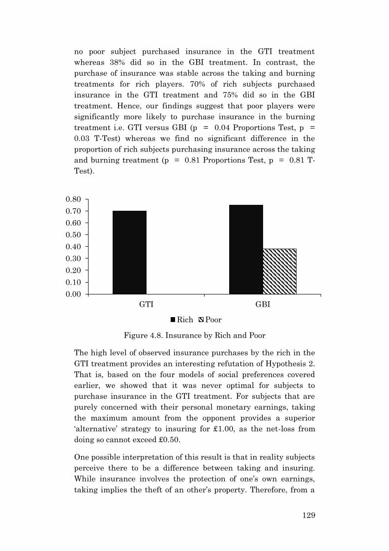
129

no poor subject purchased insurance in the GTI treatment

whereas 38% did so in the GBI treatment. In contrast, the

purchase of insurance was stable across the taking and burning

treatments for rich players. 70% of rich subjects purchased

insurance in the GTI treatment and 75% did so in the GBI

treatment. Hence, our findings suggest that poor players were

significantly more likely to purchase insurance in the burning

treatment i.e. GTI versus GBI (p = 0.04 Proportions Test, p =

0.03 T-Test) whereas we find no significant difference in the

proportion of rich subjects purchasing insurance across the taking

and burning treatment (p = 0.81 Proportions Test, p = 0.81 T-

Test).

Figure 4.8. Insurance by Rich and Poor

The high level of observed insurance purchases by the rich in the

GTI treatment provides an interesting refutation of Hypothesis 2.

That is, based on the four models of social preferences covered

earlier, we showed that it was never optimal for subjects to

purchase insurance in the GTI treatment. For subjects that are

purely concerned with their personal monetary earnings, taking

the maximum amount from the opponent provides a superior

‘alternative’ strategy to insuring for £1.00, as the net-loss from

doing so cannot exceed £0.50.

One possible interpretation of this result is that in reality subjects

perceive there to be a difference between taking and insuring.

While insurance involves the protection of one’s own earnings,

taking implies the theft of an other’s property. Therefore, from a

0.00

0.10

0.20

0.30

0.40

0.50

0.60

0.70

0.80

GTI GBI

Rich Poor

130

psychological perspective, there is an important distinction

between these two options. Moreover, as subjects don’t know with

any certainty the strategy of their opponent, insurance provides

them with the ability to completely eliminate uncertainty. This is

important not only from a financial standpoint i.e. by removing

uncertainty regarding final payoffs, but is also important for

behavioural reasons.

Specifically, if the subject expects their opponent to take with

some positive probability and chooses take as an alternative

strategy to insuring, then there is still a possibility that their

expectation was incorrect, in which case taking from a poor

subject who in fact hadn’t decided to take may lead to feelings of

guilt and regret for the richer player. Hence, although the four

models of social preferences presented earlier may not capture

such motives, the high levels of observed insurance may have

been driven by a combination of emotional and property-right

based reasoning.

4.5.5. Do Nothing

Finding 9: We observe a significant increase in the fraction of

subjects that chose to do nothing and a simultaneous reduction in

the fraction of subjects that took in the GB treatment relative to

the GT treatment.

The proportion of subjects that decided to do nothing rose from

32% in the GT treatment to 60% in the GB treatment (p = 0.07

Proportions Test, p = 0.06 T-Test). In contrast, the fraction of

subjects that decided to take fell from 45% in the GT treatment to

25% in the GB treatment (taking in the GT versus GB treatment,

p = 0.17 Proportions Test, p = 0.17 T-Test) while the difference

in the level of giving was far less pronounced as 15% of subjects

gave in the GB treatment compared to 23% in the GT treatment

(p = 0.52 Proportions-Test, p = 0.53 T-Test).

Since burning money under all circumstances implied a net

monetary cost to the taker, this finding suggests that part of our

subject pool was indeed motivated purely by self-interest. This

provides some support towards Hypothesis 1 and the predictions

derived from the model of narrow self-interest.

131

Finding 10: Extending the choice-set to include the option to

insure significantly lowers the fraction of subjects that choose to

do nothing.

Comparing the incidence of choosing to do nothing across the

insurance and no insurance treatments, we find a significant

reduction from 45% of subjects in the no insurance treatment to

22% of subjects choosing to do nothing in the insurance treatment

(p = 0.03 Proportions Test, p = 0.03 T-Test). Moreover, the

fraction of rich subjects that chose to do nothing fell substantially

from 43% in the no insurance treatment to 6% in the insurance

treatment (p = 0.01 Proportions Test, p = 0.00 T-Test) whilst

the fraction of poor subjects that chose to do nothing fell

insignificantly from 48% in the no insurance treatment to 39% in

the insurance treatment (p = 0.58 Proportions Test, p = 0.57 T-

Test).

Findings 2, 4 and 10 jointly show that expanding the available

choice-set by including the option to insure resulted in a

significant reduction in the fraction of subjects that chose to give

and do nothing but had no effect on the proportion of subjects that

decided to take. One possible interpretation of this result is that

the shift towards insurance was primarily driven by a reduction

in the proportion of subjects that decided to do nothing coupled

with the crowding out of giving, and so a reduction in prosocial

behaviour, whilst having no impact on taking. Given that we also

found a decrease in the fraction of subjects that gave the

maximum amount to their opponents in the burning treatment

relative to the taking treatment whilst finding no significant

difference in the fraction of subjects that took the maximum

amount (see Finding 6), these results imply that the preference

for altruism or acting upon advantageous inequality-aversion is

relatively weaker and less stable than the desire to mitigate

disadvantageous inequality (Messick and Sentis (1985),

Loewenstein et al. (1989) and Fehr and Schmidt (1999)). More

broadly, this result highlights the fact that altering the choice-set

available to subjects can have an impact on the degree of

altruism, as shown in several previous studies (List (2007),

Bardsley (2008)).

The data in Figure 4.1 shows that overall, around 35% of subjects

decided to do nothing. While doing nothing can certainly

represent selfishness or reciprocity motives, another potentially

132

relevant explanation for this option being chosen so frequently

could be related to the perception of fairness regarding the way in

which the endowment was earned. For example, Akbas, Ariely

and Yuksel (2014) argue that the perceived fairness of income

distributions depends on the beliefs about the process that

generated the inequality. Specifically, they outline two crucial

factors of the process that affect fairness views. These are

procedural justice i.e. equal treatment of all participants and

agency i.e. one’s ability to make their own choices. If people feel

they were treated fairly and received compensation for what they

earned, then they may choose to do nothing. In other words, the

inequality in our experiment, unlike several previous studies,

could be considered a fair and natural outcome in which rewards

were distributed according to differences in performance. This

could potentially affect the incentive of subjects to counter such

inequality.

4.5.6. Gender

There is considerable experimental evidence to suggest that

gender is an important determinant of a variety of economic and

strategic decisions (Eckel and Grossman 1998, Croson and Gneezy

2009), and on subjects’ beliefs about the altruistic behaviour of

men and women (Aguiar et al. 2009). Chowdhury et al. (2016) run

a dictator game with both give and take frames finding that

females allocate significantly more under the taking frame than

in the giving frame whereas males display the exact opposite

behaviour. The authors argue that using a taking frame makes

male subjects significantly more selfish while making females

more egalitarian, in comparison to the giving frame. More

generally, females have been found to display greater altruism

than their male counterparts in dictator games (see Engel 2011

for a review).

Findings from the literature cited above could translate into

gender differences between a take-and-keep and take-and-burn

treatment. Experimental studies on gender differences in anti-

social behaviour are limited. Abbink and Hermann (2011) and

Kessler et al. (2012) find no evidence of a gender-effect in

antisocial behaviour. However, Ghiglieri (1999) showed in a non-

experimental study that males tend to display more aggression in

comparison to females. Hence, we test whether the context of the

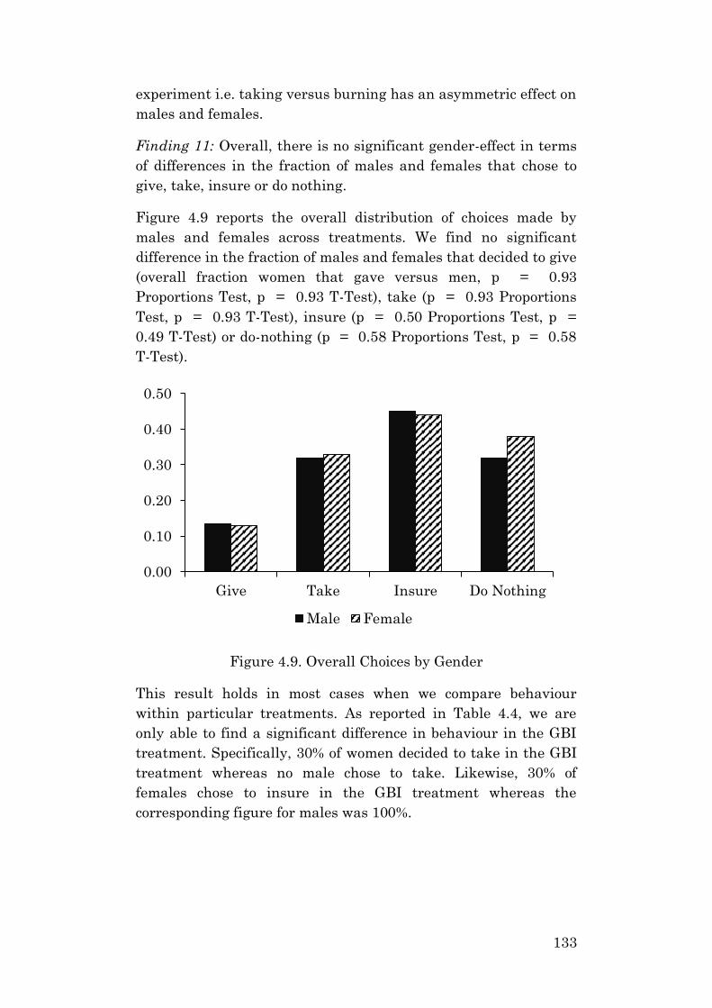
133

experiment i.e. taking versus burning has an asymmetric effect on

males and females.

Finding 11: Overall, there is no significant gender-effect in terms

of differences in the fraction of males and females that chose to

give, take, insure or do nothing.

Figure 4.9 reports the overall distribution of choices made by

males and females across treatments. We find no significant

difference in the fraction of males and females that decided to give

(overall fraction women that gave versus men, p = 0.93

Proportions Test, p = 0.93 T-Test), take (p = 0.93 Proportions

Test, p = 0.93 T-Test), insure (p = 0.50 Proportions Test, p =

0.49 T-Test) or do-nothing (p = 0.58 Proportions Test, p = 0.58

T-Test).

Figure 4.9. Overall Choices by Gender

This result holds in most cases when we compare behaviour

within particular treatments. As reported in Table 4.4, we are

only able to find a significant difference in behaviour in the GBI

treatment. Specifically, 30% of women decided to take in the GBI

treatment whereas no male chose to take. Likewise, 30% of

females chose to insure in the GBI treatment whereas the

corresponding figure for males was 100%.

0.00

0.10

0.20

0.30

0.40

0.50

Give Take Insure Do Nothing

Male Female

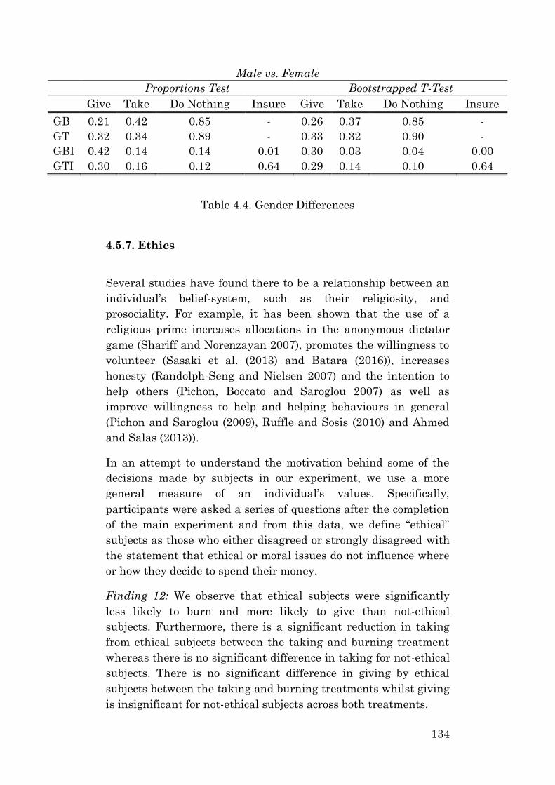
134

Male vs. Female

Proportions Test Bootstrapped T-Test

Give Take Do Nothing Insure Give Take Do Nothing Insure

GB 0.21 0.42 0.85 - 0.26 0.37 0.85 -

GT 0.32 0.34 0.89 - 0.33 0.32 0.90 -

GBI 0.42 0.14 0.14 0.01 0.30 0.03 0.04 0.00

GTI 0.30 0.16 0.12 0.64 0.29 0.14 0.10 0.64

Table 4.4. Gender Differences

4.5.7. Ethics

Several studies have found there to be a relationship between an

individual’s belief-system, such as their religiosity, and

prosociality. For example, it has been shown that the use of a

religious prime increases allocations in the anonymous dictator

game (Shariff and Norenzayan 2007), promotes the willingness to

volunteer (Sasaki et al. (2013) and Batara (2016)), increases

honesty (Randolph-Seng and Nielsen 2007) and the intention to

help others (Pichon, Boccato and Saroglou 2007) as well as

improve willingness to help and helping behaviours in general

(Pichon and Saroglou (2009), Ruffle and Sosis (2010) and Ahmed

and Salas (2013)).

In an attempt to understand the motivation behind some of the

decisions made by subjects in our experiment, we use a more

general measure of an individual’s values. Specifically,

participants were asked a series of questions after the completion

of the main experiment and from this data, we define “ethical”

subjects as those who either disagreed or strongly disagreed with

the statement that ethical or moral issues do not influence where

or how they decide to spend their money.

Finding 12: We observe that ethical subjects were significantly

less likely to burn and more likely to give than not-ethical

subjects. Furthermore, there is a significant reduction in taking

from ethical subjects between the taking and burning treatment

whereas there is no significant difference in taking for not-ethical

subjects. There is no significant difference in giving by ethical

subjects between the taking and burning treatments whilst giving

is insignificant for not-ethical subjects across both treatments.

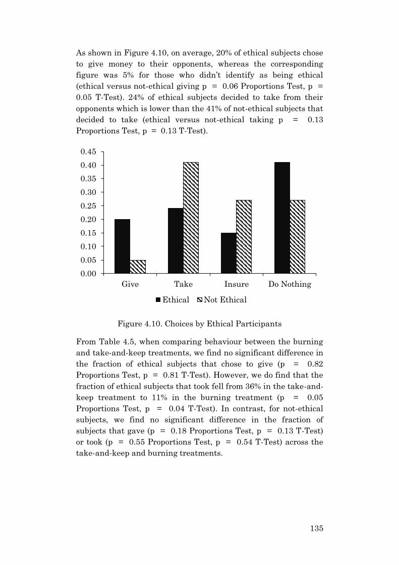
135

As shown in Figure 4.10, on average, 20% of ethical subjects chose

to give money to their opponents, whereas the corresponding

figure was 5% for those who didn’t identify as being ethical

(ethical versus not-ethical giving p = 0.06 Proportions Test, p =

0.05 T-Test). 24% of ethical subjects decided to take from their

opponents which is lower than the 41% of not-ethical subjects that

decided to take (ethical versus not-ethical taking p = 0.13


Figure 4.10. Choices by Ethical Participants

From Table 4.5, when comparing behaviour between the burning

and take-and-keep treatments, we find no significant difference in

the fraction of ethical subjects that chose to give (p = 0.82

Proportions Test, p = 0.81 T-Test). However, we do find that the

fraction of ethical subjects that took fell from 36% in the take-and-

keep treatment to 11% in the burning treatment (p = 0.05

Proportions Test, p = 0.04 T-Test). In contrast, for not-ethical

subjects, we find no significant difference in the fraction of

subjects that gave (p = 0.18 Proportions Test, p = 0.13 T-Test)

or took (p = 0.55 Proportions Test, p = 0.54 T-Test) across the

take-and-keep and burning treatments.

0.00

0.05

0.10

0.15

0.20

0.25

0.30

0.35

0.40

0.45


Ethical Not Ethical

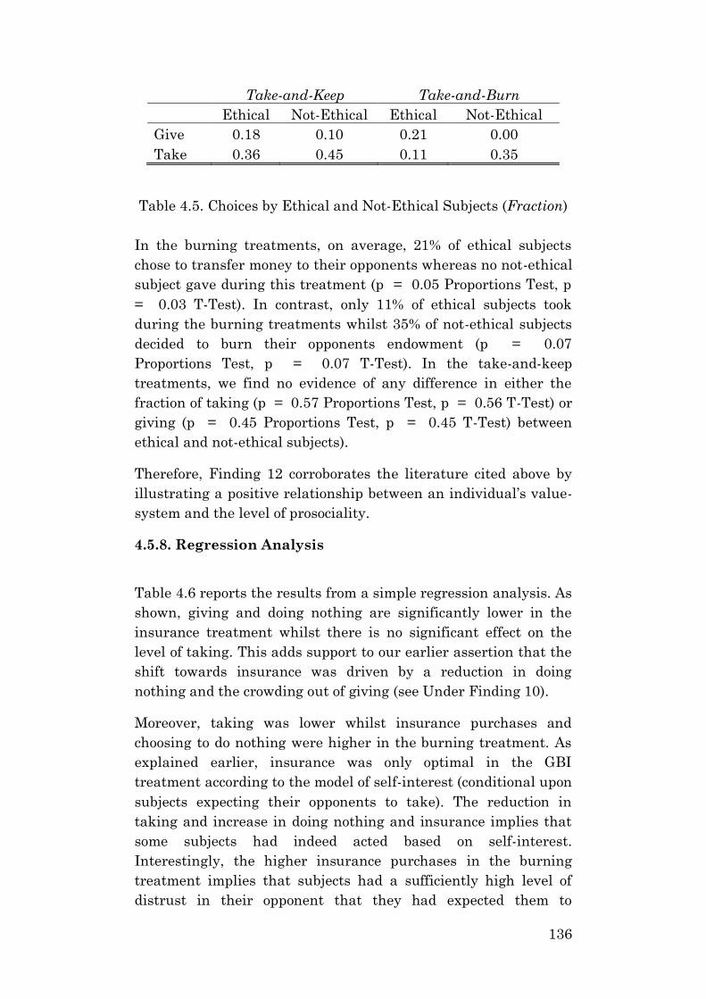
136

Take-and-Keep Take-and-Burn

Ethical Not-Ethical Ethical Not-Ethical

Give 0.18 0.10 0.21 0.00

Take 0.36 0.45 0.11 0.35

Table 4.5. Choices by Ethical and Not-Ethical Subjects (Fraction)

In the burning treatments, on average, 21% of ethical subjects

chose to transfer money to their opponents whereas no not-ethical

subject gave during this treatment (p = 0.05 Proportions Test, p

= 0.03 T-Test). In contrast, only 11% of ethical subjects took

during the burning treatments whilst 35% of not-ethical subjects

decided to burn their opponents endowment (p = 0.07

Proportions Test, p = 0.07 T-Test). In the take-and-keep

treatments, we find no evidence of any difference in either the

fraction of taking (p = 0.57 Proportions Test, p = 0.56 T-Test) or

giving (p = 0.45 Proportions Test, p = 0.45 T-Test) between

ethical and not-ethical subjects).

Therefore, Finding 12 corroborates the literature cited above by

illustrating a positive relationship between an individual’s value-

system and the level of prosociality.

4.5.8. Regression Analysis

Table 4.6 reports the results from a simple regression analysis. As

shown, giving and doing nothing are significantly lower in the

insurance treatment whilst there is no significant effect on the

level of taking. This adds support to our earlier assertion that the

shift towards insurance was driven by a reduction in doing

nothing and the crowding out of giving (see Under Finding 10).

Moreover, taking was lower whilst insurance purchases and

choosing to do nothing were higher in the burning treatment. As

explained earlier, insurance was only optimal in the GBI

treatment according to the model of self-interest (conditional upon

subjects expecting their opponents to take). The reduction in

taking and increase in doing nothing and insurance implies that

some subjects had indeed acted based on self-interest.

Interestingly, the higher insurance purchases in the burning

treatment implies that subjects had a sufficiently high level of

distrust in their opponent that they had expected them to

137

willingly incur a net personal cost in order to sabotage their

earnings. From the perspective of a rich player, ex-post, the

purchase of insurance during the GBI treatment seems justified

based on our findings on the behaviour of poor subjects in the

burn treatment.

Our results show that poor subjects were significantly less likely

to have purchased insurance and give money but more likely to

have taken in comparison to rich subjects. Finding 5 showed that

there was no significant difference in taking by the poor between

the take and burn treatments. Hence, from our earlier predictions

(see Table 4.3), these results suggest that the models of

inequality-aversion and envy provide a more accurate description

of the observed behaviour of poorer subjects in comparison to the

model of narrow self-interest. In combination with Findings 1 and

5, we observe evidence of both altruism and selfishness from rich

players.

Risk-aversion is an important determinant of the demand for

insurance (see Outreville 2013). Risk-averse agents agree to pay

an insurance premium that is in excess of the mathematical

expectation of loss29. Numerous studies have documented

evidence of agents displaying some positive degree of risk-

aversion (Gneezy and Potters (1997), Eckel and Grossman (2002)

and Holt and Laury (2002)). Table 4.6 shows that the purchase of

insurance was higher for those that self-reported a higher degree

of risk-aversion30 as well as for those that had expected to be

taken from. This result indicates that a key determinant of

insurance demand was the desire for greater certainty regarding

the final allocation of subject endowments.

29 The maximum amount of money that can be taken from any

subject is £2.50. If a player anticipates this, they would be better

off (in the GTI treatment) taking an equal amount from their

opponent which would leave both 50p worse off. However, the

purchase of insurance at £1.00 would be indicative of risk-

aversion as it would suggest that subjects were willing to pay a

premium in order to ensure they have certainty regarding their

final payoff. 30 Risk-aversion here is based on a self-reported measure where

subjects were asked to rank their appetite for risk on a scale

ranging from 1-10 with 1 being fully risk-averse and 10

representing a risk-lover.

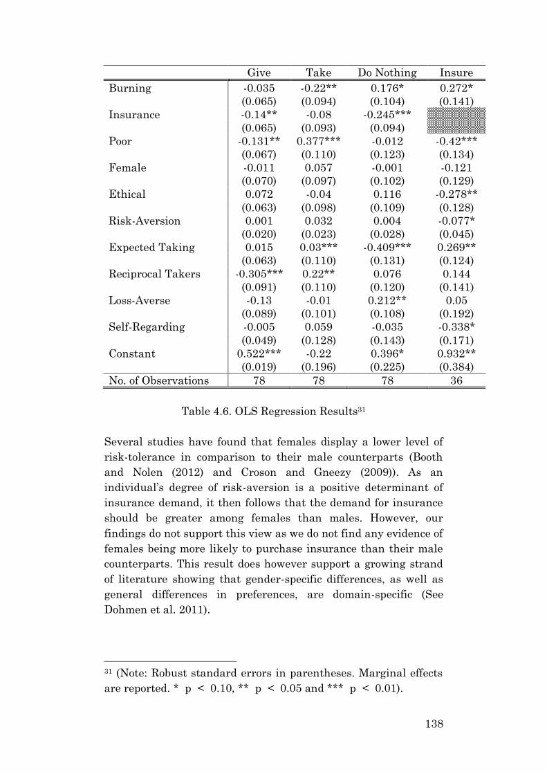
138

Give Take Do Nothing Insure

Burning -0.035 -0.22** 0.176* 0.272*

(0.065) (0.094) (0.104) (0.141)

Insurance -0.14** -0.08 -0.245***

(0.065) (0.093) (0.094)

Poor -0.131** 0.377*** -0.012 -0.42***

(0.067) (0.110) (0.123) (0.134)

Female -0.011 0.057 -0.001 -0.121

(0.070) (0.097) (0.102) (0.129)

Ethical 0.072 -0.04 0.116 -0.278**

(0.063) (0.098) (0.109) (0.128)

Risk-Aversion 0.001 0.032 0.004 -0.077*

(0.020) (0.023) (0.028) (0.045)

Expected Taking 0.015 0.03*** -0.409*** 0.269**

(0.063) (0.110) (0.131) (0.124)

Reciprocal Takers -0.305*** 0.22** 0.076 0.144

(0.091) (0.110) (0.120) (0.141)

Loss-Averse -0.13 -0.01 0.212** 0.05

(0.089) (0.101) (0.108) (0.192)

Self-Regarding -0.005 0.059 -0.035 -0.338*

(0.049) (0.128) (0.143) (0.171)

Constant 0.522*** -0.22 0.396* 0.932**

(0.019) (0.196) (0.225) (0.384)

No. of Observations 78 78 78 36

Table 4.6. OLS Regression Results31

Several studies have found that females display a lower level of

risk-tolerance in comparison to their male counterparts (Booth

and Nolen (2012) and Croson and Gneezy (2009)). As an

individual’s degree of risk-aversion is a positive determinant of

insurance demand, it then follows that the demand for insurance

should be greater among females than males. However, our

findings do not support this view as we do not find any evidence of

females being more likely to purchase insurance than their male

counterparts. This result does however support a growing strand

of literature showing that gender-specific differences, as well as

general differences in preferences, are domain-specific (See

Dohmen et al. 2011).

31 (Note: Robust standard errors in parentheses. Marginal effects

are reported. * p < 0.10, ** p < 0.05 and *** p < 0.01).

139

Traditional economic theory posits that immoral behaviour, such

as lying and stealing, is a product of both income effects and the

probability of being caught and punished (Becker 1968). More

recently, this standard theory has been questioned with the

concept of non-pecuniary moral costs associated with lying and

stealing being incorporated into the decision model (Gneezy

(2005), Levitt and List (2007), Fischbacher and Heusi (2008),

Mazar et al. (2008) and Lundquist et al. (2009)). In a sense, the

standard assumption can be thought of as being based on the

assumption that agents are self-regarding. In an attempt to

capture agents who behave in such a manner, we asked subjects

in our post-experiment questionnaire whether they felt that it

was justified to do anything in the pursuit of success as long as

they could get away with their actions. Subjects that either

agreed or strongly agreed with this statement were labelled as

being “self-regarding”.

We consider the variable “ethical” introduced earlier a proxy for

those that are more likely to take into consideration the non-

pecuniary costs of stealing. From Table 4.6, we see that both

ethical and self-regarding participants were significantly less

likely to purchase insurance. Although we are unable to find

statistical significance in any other regression for these two

variables, it is interesting to note that our results show a negative

coefficient on giving and doing nothing but a positive coefficient

on taking for self-regarding subjects. In contrast, we find the

complete opposite for ethical subjects whereby the coefficients on

giving and doing nothing are positive whilst the coefficient on

taking is negative.

As in Finding 12, this result suggests that part of the observed

heterogeneity in preferences is likely to be based upon an

individual’s ethical and moral code. Ethical subjects are more

likely to behave altruistically by donating a portion of their

endowments to their poorer opponents and less likely to steal

from their opponent. Based on self-reported responses, self-

regarding subjects are willing to behave antisocially by engaging

in activities, albeit illicit, in order to improve their own situation.

Subjects were also asked in the post-experiment questionnaire

how they would have responded if they were told with complete

certainty that their opponent had chosen to take money from

them. Participants that either agreed or strongly agreed that they

140

would have also chosen to take money from their opponent were

categorised as “reciprocal takers”. Note that there is a distinction

between those that had expected to be taken from and those that

would reciprocate taking. While the former may have also

responded by taking during the experiment, their decision was

based on an expectation regarding their opponent’s strategy. In

comparison, reciprocal taking is based upon a hypothetical

scenario in which there is complete certainty regarding the

opponent’s actions. Therefore, whilst those that were categorised

as reciprocal takers may have also expected their opponent to

have taken during the experiment, the probability they had

assigned to their opponent choosing to take may have been

sufficiently low so as to have prevented them from taking during

the experiment.

Table 4.6 shows that those expecting to be taken from were

significantly less likely to do nothing and more likely to take and

purchase insurance Reciprocal takers were significantly less

likely to give and more likely to take. We do not find a significant

insurance effect for reciprocal takers. However, we find that the

coefficient for reciprocal takers in the taking regression is over

seven times higher than that on those that expected to be taken

from.

This result reinforces our assertion under Finding 8 that the high

levels of insurance purchases observed in the GTI game may have

been a consequence of uncertainty regarding the opponent’s

choice. In order to avoid the regret or guilt of taking from an

opponent that didn’t take, subjects may have opted for insurance.

In other words, at least some subjects that had an expectation of

being taken from didn’t have an expectation that was sufficiently

high to trigger taking i.e. the optimal strategy in monetary terms.

Hence, such subjects may have rather opted to purchase

insurance.

4.5.9. Insurance and Welfare

Comparing the average payoffs across treatments for rich and

poor subjects (see Table 4.7), our results show an insignificant

increase in the average payoff for rich subjects from £13.68 in the

no insurance treatment to £13.90 in the insurance treatment (p =

0.40 Mann-Whitney, p = 0.64 T-Test), an increase from £13.56 in

141

the GT treatment to £13.74 GTI treatment (p = 0.43 Mann-

Whitney, p = 0.83 T-Test) and an increase from £13.81 in the GB

treatment to £14.10 in the GBI treatment (p = 0.44 Mann-

Whitney, p = 0.78 T-Test). However, we do find weak evidence

that the availability of insurance influences the average payoff for

poor subjects. Specifically, the average payoff fell from £5.33 in

the no insurance treatment to £4.94 in the insurance treatment (p

= 0.10 Mann-Whitney, p = 0.39 T-Test), from £5.85 in the GT

treatment to £5.20 in the GTI treatment (p = 0.20 Mann-

Whitney, p = 0.39 T-Test) and fell from £4.77 in the GB

treatment to £4.61 in the GBI treatment (p = 0.27 Mann-

Whitney, p = 0.60 T-Test).

There is weak evidence to support the notion that the availability

of insurance worsens inequality. From earlier results, we found

that the availability of insurance had no significant impact on

taking but led to a reduction in the fraction of rich players that

chose to give and do nothing. Moreover, we reported a high and

significant uptake of insurance by the rich. This implies that the

shift towards insurance was partially driven by a reduction in the

fraction of rich subjects that chose to do nothing and the crowding

out of giving. Coupled with the inability of poor players to access

the endowment of the insured rich and the fact that we find no

difference in taking by the poor across the insurance and no

insurance treatments, these factors may provide an explanation

for the observed fall in the average payoff of poor subjects and the,

albeit insignificant, increase in the average payoff of richer

subjects.

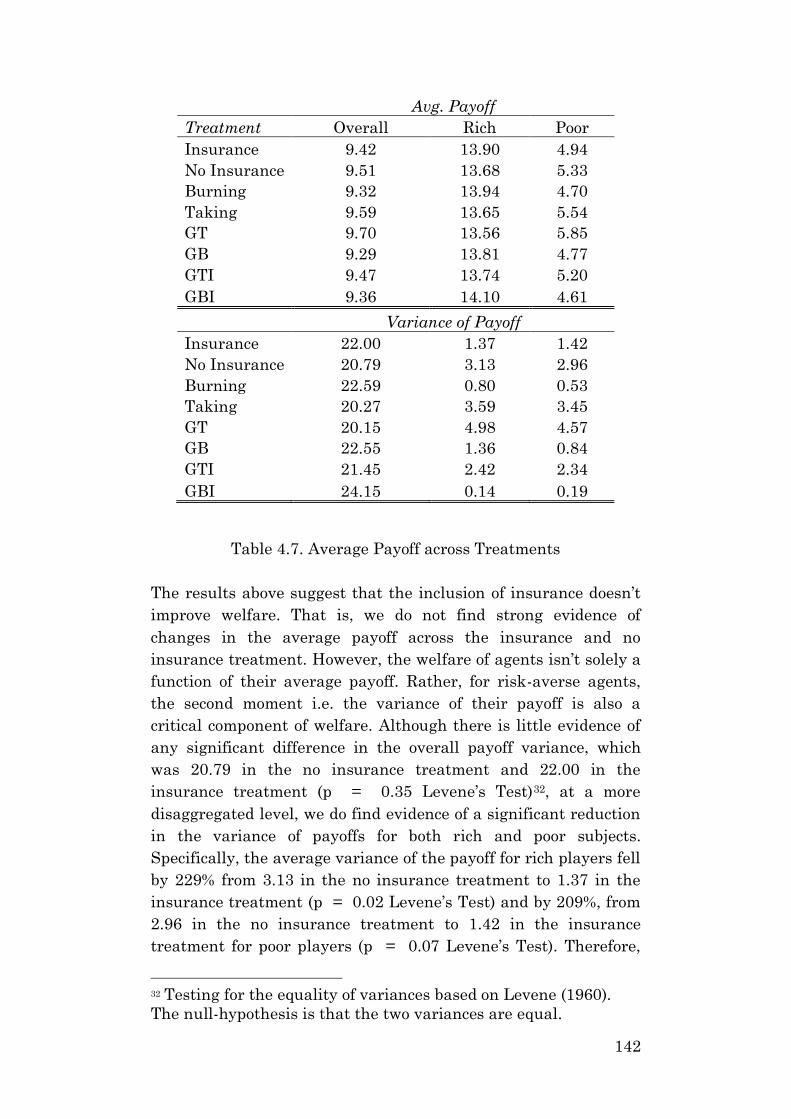
142

Avg. Payoff

Treatment Overall Rich Poor

Insurance 9.42 13.90 4.94

No Insurance 9.51 13.68 5.33

Burning 9.32 13.94 4.70

Taking 9.59 13.65 5.54

GT 9.70 13.56 5.85

GB 9.29 13.81 4.77

GTI 9.47 13.74 5.20

GBI 9.36 14.10 4.61

Variance of Payoff

Insurance 22.00 1.37 1.42

No Insurance 20.79 3.13 2.96

Burning 22.59 0.80 0.53

Taking 20.27 3.59 3.45

GT 20.15 4.98 4.57

GB 22.55 1.36 0.84

GTI 21.45 2.42 2.34

GBI 24.15 0.14 0.19

Table 4.7. Average Payoff across Treatments

The results above suggest that the inclusion of insurance doesn’t

improve welfare. That is, we do not find strong evidence of

changes in the average payoff across the insurance and no

insurance treatment. However, the welfare of agents isn’t solely a

function of their average payoff. Rather, for risk-averse agents,

the second moment i.e. the variance of their payoff is also a

critical component of welfare. Although there is little evidence of

any significant difference in the overall payoff variance, which

was 20.79 in the no insurance treatment and 22.00 in the

insurance treatment (p = 0.35 Levene’s Test)32, at a more

disaggregated level, we do find evidence of a significant reduction

in the variance of payoffs for both rich and poor subjects.

Specifically, the average variance of the payoff for rich players fell

by 229% from 3.13 in the no insurance treatment to 1.37 in the

insurance treatment (p = 0.02 Levene’s Test) and by 209%, from

2.96 in the no insurance treatment to 1.42 in the insurance

treatment for poor players (p = 0.07 Levene’s Test). Therefore,

32 Testing for the equality of variances based on Levene (1960).

The null-hypothesis is that the two variances are equal.

143

despite there being no significant change in average payoffs, if the

payoff variance is used as a measure of risk, then the average

payoff per unit of risk i.e. average payoff divided by average

variance increased from 7.73 in the no insurance treatment to

11.88 in the insurance treatment for rich subjects and from 3.10

to 4.15 for poor subjects.


Theories of other-regarding preferences typically predict that

giving increases with an individual’s income. This has been

attributed to various factors such as relative earnings (Bolton

1991), inequality-aversion (Fehr and Schmidt (1999), Bolton and

Ockenfels (2000) and Alesina and Angeltos (2005)) and warm glow

(Andreoni 1990). There exists a voluminous literature reinforcing

the idea of positive other-regarding preferences by showing the

existence of prosocial behaviour in the lab (Andreoni et al. (2007)

and Engel (2011)). The more recent literature has found

conflicting evidence of antisocial behaviour in the lab e.g. theft

and sabotage of an opponent’s earnings. It has been argued that

this so-called dark-side of human behaviour is motivated by

inequality-aversion, envy and pure nastiness (Zizzo and Oswald

(2001) and Abbink and Sadrieh (2009)).

Developing a better understanding of antisocial preferences can

provide valuable insights33. This is because the forces of spite and

envy have been argued to have both socially destructive and

constructive ramifications. If agents are willing to expend

resources to undermine the performance and success of others

33 A potentially interesting extension of our work, that is not

explored here, could be to provide insight into the weight of 𝜃 on

the opponent’s monetary gain and the range of its parameter

value. For example, perhaps a separable preference that nests

both an other-regarding and stealing aversion component such as:

𝑈(𝐶𝑜𝑤𝑛) − 𝜃𝑈(𝐶𝑜𝑡ℎ𝑒𝑟) + 𝛾1𝑠𝑡𝑒𝑎𝑙

Assuming an arbitrarily large dataset, one should be able to

reveal the parameter values of both 𝜃 and 𝛾.

144

(Smith and Kim (2007) and Van de Ven, Zeelenberg and Pieters

(2009)), then such behaviour could negatively impact societal

cohesion and welfare as well as discouraging investment and

productivity (Kebede and Zizzo 2015). On the other hand, envy

has the potential to serve as a motivator for the envious to work

harder in order to progress in the income and status hierarchies

(Grolleau et al. 2009).

Evidence regarding the impact of income inequality (which has

been argued to be a major driver of spite and envy) on behaviour

has been mixed. For instance, while it has been found that low-

income subjects are relatively more co-operative than their high-

income counterparts (Buckley and Croson 2006), other studies

have shown there to be little difference between the willingness to

harm others among low and high income subjects (Grossman and

Komai 2016). With the growing levels of inequality across several

countries (Piketty 2014), it has been argued that the social and

economic consequences have become more pertinent to

understand.

More broadly, it has been shown that competitive environments

can encourage sabotage (Charness et al. (2011), Balafoutas et al.

(2012) and Jauernig and Uhl (2019)). For example, Harbring and

Irlenbusch (2011) use an experimental tournament setting to

show that wage differences between subjects increases sabotage.

Gurr (1970) argues that the opportunity costs of the relatively

disadvantaged decreases while their inclination to engage in

violent demands for redistribution increases following an increase

in inequality. Given that people may in general have some

tendency to envy those that are in a better position than

themselves (Tullock 2013), it is of interest to study the role of

inequality derived from differences in performance on the

behaviour of agents.

In this study, we ran a simple incentivised laboratory experiment

to test whether altering subject choice-sets and the context in

which the decision is made (i.e. take-and-keep versus take-and-

burn) influences the level of prosociality after subjects have

competed in a tournament setting. Consistent with previous

findings, our results suggest that some agents do display other-

regarding preferences. However, we not only observe

heterogeneity in preferences across subjects but also find that

behaviour can be sensitive to changes in the exact context and

145

choice-set presented to subjects (List (2007), Bardsley (2008) and

Dohmen et al. (2011)).

We report evidence showing that altering subject choice-sets had

an asymmetric effect on attitudes. Our data shows that an

expansion of the available choice-set to include the option of

insurance crowds out donations from competition winners (rich

subjects) and shifting from the take-and-keep to the take-and-

burn treatment lowered the average size of donations. We find a

high and significant uptake of insurance by tournament winners

even in cases in which insuring was a dominated strategy in

monetary terms. One interpretation of this finding is that rich

subjects avoided stealing from poorer opponents due to

uncertainty regarding their chosen action. Specifically, rich

subjects may have preferred to incur an additional £0.50 cost to

purchase insurance in order to avoid the ex-post regret or guilt of

having taken from a poor opponent that didn’t choose to take.

In contrast, our results show that neither an expansion of the

choice-set nor a switch from the take-and-keep treatment to the

take-and-burn treatment impacted taking by competition losers

(poor subjects). This was both in terms of the fraction of poor

subjects that took and the size of the amounts taken. Hence, we

found that the aforementioned changes to the decision-task were

more effective at lowering prosocial behaviour by competition

winners whilst being less effective at having any impact on the

antisocial behaviour of competition losers.

In combination with the prior literature, an important

overarching implication of our findings is that the situational

instability of preferences observed in the lab is likely responsible

for the lack of external validity of experimental studies. While the

experimental literature has provided valuable insights through

theory-testing, in order to address concrete real-world problems

there is a need for greater emphasis on context-specific studies,

the results of which may only have limited scope in terms of

generalizability (see Guala and Mittone 2005).

146

4.7. REFERENCES

1. Abbink, K. and Herrmann, B. (2009). Pointless vendettas.

Working Paper Series, University of East Anglia, Centre

for Behavioural and Experimental Social Science.

2. Abbink, K. and Herrmann, B. (2011). The moral costs of

nastiness. Economic Inquiry, 49(2), 631-633.

3. Abbink, K. and Sadrieh, A. (2009). The pleasure of being

nasty. Economics Letters, 105(3), 306-308

4. Abbink, K., Masclet, D. and Van Veelen, M. (2011).

Reference point effects in antisocial preferences. CIRANO

Scientific Publications No. 2011s-11.

5. Aguiar, F., Branas-Garza, P., Cobo-Reyes, R., Jimenez, N.

and Miller, L.M. (2009). Are women expected to be more

generous? Experimental Economics, 12(1), 93-98.

6. Ahmed, A. and Salas, O. (2013). Religious context and

prosociality: An experimental study from Valparaiso, Chile.

Journal for the Scientific Study of Religion, 52(3), 627-637.

7. Akbas, M., Ariely, D. and Yuksel, S. (2016). When is

inequality fair? An experiment on the effect of procedural

justice and agency. Mimeo.

8. Alesina, A. and Angeletos, G.M. (2005). Fairness and

redistribution: US vs. Europe. American Economic Review,

95(4), 913-935.

9. Alm, J., Sanchez, I. and de Juan, A. (1995). Economic and

non-economic factors in tax compliance. Kyklos, 48(1), 3-18.

10. Andreoni, J., Harbaugh, W.T. and Vesterlund, L. (2007).

Altruism in Experiments. In the New Palgrave Dictionary

of Economics (2nd edition).

11. Andreoni, J. (1990). Impure altruism and donations to

public goods: A theory of warm-glow giving. Economic

Journal, 100(401), 464-477.

12. Andreoni, J. and Miller, J.H. (2002). Giving according to

GARP: An experimental study of rationality and altruism.

Econometrica, 70, 737-753.

13. Arrow, K.J. (1981). Optimal and voluntary income

redistribution. In: Rosenfield, S. (Ed.), Economic Welfare

and the Economics of Soviet Socialism: Essays in Honor of

Abram Bergson, Cambridge University Press.

147

14. Balafoutas, L., Linder, F. and Sutter, M. (2012). Sabotage

in tournaments: Evidence from a natural experiment.

Kyklos, 65, 425-441.

15. Bandiera, O., Barankay, I. and Rasul, I. (2005). Social

preferences and the response to incentives: Evidence from

personnel data. Quarterly Journal of Economics, 120(3),

917-962.

16. Bardsley, N. (2008). Dictator game giving: altruism or

artefact? Experimental Economics, 11(2), 122-133.

17. Batara J. B. L. (2016). Religious song as a facilitator of

prosocial behavior. International Journal of Research

Studies in Psychology, 5(1), 3–12.

18. Bault, N., Coricelli, G. and Rustichini, A. (2008).

Interdependent utilities: How social ranking affects choice

behaviour, PLoS One, 3(10),

19. Becker, G.S. (1968). Crime and punishment: an economic

approach. Journal of Political Economy, 76(2), 169-217.

20. Becker, G.S. (1974). A theory of social interactions. Journal

of Political Economy, 82, 1063-1093.

21. Beckman, S.R., Formby, J.P., Smith, W.J. and Zheng, B.

(2002). Envy, malice and Pareto efficiency: An experimental

investigation. Social Welfare, 19, 349-367.

22. Bellemare, C., Kroger, S. and Van Soest, A. (2008).

Measuring inequity aversion in a heterogeneous population

using experimental decisions and subjective probabilities.

Econometrica, 76(4), 815-839.

23. Benz, M. and Meier, S. (2008). Do people behave in

experiments as in the field? Evidence from donations.

Experimental Economics, 11(3), 268-281.

24. Blanco, M., Engelmann, D. and Normann, H. T. (2011). A

within-subject analysis of other-regarding preferences.

Games and Economic Behaviour, 72, 321-338.

25. Bognanno, M. (2001). Corporate tournaments. Journal of

Labor Economics, 19(2), 290-315.

26. Bohnet, I. and Frey, B.S. (1999). Social distance and other-

regarding behaviour in dictator games. American Economic

Review, 89(1), 335-339.

27. Bolton, G.E. and Ockenfels, A. (2000). A theory of equity,

reciprocity and competition. American Economic Review,

90, 166-193.

28. Bothner, M., Kang, J. and Stuart, T. (2007). Competitive

crowding and risk taking in a tournament: evidence from

148

NASCAR racing. Administrative Science Quarterly, 52(2),

208-247.

29. Branas-Garza, P., Duran, M.A. and Espinosa, M.P. (2012).

Favouring friends. Bulletin of Economic Research, 64(2),

174-178.

30. British Crime Survey. (2016). Crime in England and

Wales: year ending March 2016. Office for National

Statistics. Statistical bulletin.

31. Brown, A.L., Meer, J. and Williams, J.F. (2018). Why do

people volunteer? An experimental analysis of preferences

for time donations. Management Science, 65(4), 1455-1468.

32. Buckley, E. and Croson, R. (2006). Income and wealth

heterogeneity in the voluntary provision of linear public

goods. Journal of Public Economics, 90(4-5), 935-955.

33. Caplan, B. (2005). What took you so long? Library

Economics Liberty, September 3, 2005.

34. Carpenter, J. and Myers, C.K. (2010). Why volunteer?

Evidence on the role of altruism, image and incentives.

Journal of Public Economics, 94(1), 911-920.

35. Carvalho, L. (2010). Poverty and Time Preference. RAND

Labor and Population Working Paper.

36. Casas-Arce, P. and Martinez-Jerez, F.A. (2009). Relative

performance compensation, contests, and dynamic

incentives. Management Science, 55(8), 1306-1320.

37. Chakravarty, S., Fonseca, M., Ghosh, S. and Marjit, S.

(2019). Religious fragmentation, social identity and

cooperation: evidence from an artefactual field experiment

in India. Journal of Behavioural and Experimental

Economics, 82, 101451.

38. Charness, G. and Rabin, M. (2002). Understanding social

preferences with simple tests. Quarterly Journal of

Economics, 117, 817-869.

39. Charness, G., Masclet, D. and Villeval, M.C. (2014). The

dark side of competition for status. Management Science,

60, 38-55.

40. Cherry, T.L., Frykblom, P. and Shogren, J.G. (2002).

Hardnose the dictator. The American Economic Review,

92(4), 1218-1221.

41. Chowdhury, S.M., Jeon, J.Y. and Saha, B. (2016). Gender

differences in the giving and taking variants of the dictator

game. Discussion Paper Series, University of East Anglia,

Centre for Behavioural and Experimental Social Science.

149

42. Clark, A.E. and Oswald, A.J. (1996). Satisfaction and

comparison income. Journal of Public Economics, 61(3),

359-381.

43. Cohen, Mark. (1998). The monetary value of saving a high-

risk youth. Journal of quantitative criminology, 14(1), 5-33.

44. Cox, J., Sadiraj, K. and Sadiraj, V. (2002). Trust, fear,

reciprocity and altruism. University of Arizona Working

Paper.

45. Croson, R. and Gneezy, U. (2009). Gender differences in

preferences. Journal of Economic Literature, 47(2), 1-27.

46. Dannenberg, A., Riechmann, T., Sturm, B. and Vogt, C.

(2007). Inequity aversion and individual behaviour in

public good games: an experimental investigation. ZEW

Discussion Paper.

47. Davis, D. and Holt, C.A. (1993), Experimental Economics:

48. Deck, C.A., Lee, J., Reyes, J., and Rosen, C. (2010).

Measuring risk-aversion on multiple tasks: Can domain

specific risk attitudes explain apparently inconsistent

behaviour? University of Arkansas, mimeo.

49. Dohmen, T., Falk, A., Huffman, D., Sunde, U., Schupp, J.,

and Wagner, G.G. (2011). Individual risk-attitudes:

measurement, determinants and behavioural consequences.

Journal of the European Economic Association, 9(3), 522-

550.

50. Durante, R., Putterman, L. and van der Weele, J. (2014).

Preferences for redistribution and perception of fairness: an

experimental study. Journal of European Economic

Association, 12(4), 1059-1086.

51. Easterlin, R. A. (1995). Will raising the incomes of all

increase the happiness of all? Journal of Economic

Behaviour and Organization, 27(1), 35-47.

52. Eckel, C. and Grossman, P.J. (1996). Altruism in

anonymous dictator games. Games and Economic

Behaviour, 16, 181-191.

53. Eckel, C., and Grossman, P.J. (2008). Men, Women and

risk-aversion: Experimental evidence. Handbook of

Experimental Economics Results, Elsevier.

54. Engel, C. (2011). Dictator Games: A meta-study.

Experimental Economics, 14(4), 583-610.

55. Erkal, N., Gangadharan, L. and Nikiforakis, N. (2011).

Relative earnings and giving in a real-effort experiment.

American Economic Review, 101(7), 3330-3348.

150

56. Fehr, D. (2018). Is increasing inequality harmful?

Experimental evidence. Games and Economic Behaviour,

107, 123-134.

57. Fehr, E. and Fischbacher, U. (2002). Why social

preferences matter – the impact of non-selfish motives on

competition, cooperation and incentives. The Economic

Journal, 112, 1-33.

58. Fehr, E. and Gachter, S. (2000). Cooperation and

punishment in public goods experiments. American

Economic Review, 90, 980-994.

59. Fehr, E. and Schmidt, K. (1999). A theory of fairness,

competition and cooperation. Quarterly Journal of

Economics, 114(3), 817-868.

60. Ferrer-i-Carbonella, A. (2005). Income and well-bring: An

empirical analysis of the comparison effect. Journal of

Public Economics, 89(5-6), 997-1019.

61. Fischbacher, U. and Heusi, F. (2008). Lies in disguise. An

experimental study on cheating. TWI Research Paper

Series.

62. Fong, C.M., Bowles, S. and Gintis, H. (2005). Behavioural

motives for income redistribution. The Australian Economic

Review, 38(3), 285-297.

63. Ghiglieri, M.P. (1999). The dark side of man: Tracing the

origins of male violence. Cambridge, MA, US: Persues

Publishing.

64. Gneezy, U. (2005). Deception: the role of consequences.

American Economic Review, 95, 384-394.

65. Grolleau, G. and Said, S. (2009). Do you prefer having more

or more than others? Survey evidence on positional

concerns in France. Journal of Economic Issues, 42(4),

1145-1159.

66. Grolleau, G., Mzoughi, N. and Sultan, A. (2009). The

impact of envy-related behaviours on development. Journal

of Economic Issues, 43, 795-802.

67. Grossman, P.J. and Komai, M. (2012). Within and across

class envy: Anti-social behaviour in hierarchical groups.

Monash University Working Paper.

68. Guala, F. and Mittone, L. (2005). Experiments in

economics: External validity and the robustness of

phenomena. Journal of Economic Methodology, 4, 495-515.

69. Gurr, T. (1970). Why men rebel. Princeton University

Press.

151

70. Harbring, C. and Irelenbusch, B. (2011). Sabotage in

tournaments: evidence from a laboratory experiment.

Management Science, 57(4), 611-627.

71. Herrmann, B. and Orzen, H. (2008). The appearance of

homo rivalis: Social preferences and the nature of rent

seeking. The Centre for Decision Research and

Experimental Economics Research Paper, School of

Economics, University of Nottingham.

72. Herrmann, B., Thoni, C. and Gachter, S. (2008). Antisocial

punishment across societies. Science, 319(5868), 1362-1367.

73. Hoffman, E. and Spitzer, M.L. (1985). Entitlements, rights

and fairness: An experimental examination of subjects’

concepts of distributive justice. Journal of Legal Studies,

14, 259-297.

74. Hoffman, E., McCabe, K. and Smith, V.L. (1996). Social

distance and other-regarding behaviour in dictator games.

The American Economic Review, 86(3), 653-660.

75. Hoffman, E., McCabe, K., Shachat, K. and Smith, V.

(1994). Preference, property rights and anonymity in

bargaining games. Games and Economic Behaviour, 7(3),

346-380.

76. House of Commons Committee of Public Accounts (HoC).

(2007). Tackling anti-social behaviour. Forty-fourth report

of session 2006-07.

77. Jauernig, J. and Uhl, M. (2019). Spite and pre-emptive

retaliation after tournaments. Journal of Economic


78. Kahneman, D. and Tversky, A. (2000). Choices, values and

frames. Princeton University Press.

79. Karakostas, A. and Zizzo, D. (2016). Compliance and the

power of authority. Journal of Economic Behaviour and

Organization, 124, 67-80.

80. Kebede, B. and Zizzo, D.J. (2015). Social preferences and

agricultural innovation: an experimental case study from

Ethiopia. World Development, 67, 267-280.

81. Kessler, E., Ruiz-Martos, M. and Skuse, D. (2012).

Destructor Game. Universitat Jaume I, Castellon, Working

Paper.

82. Kirchsteiger, G. (1994). The role of envy in ultimatum

games. Journal of Economic Behaviour and Organization,

25, 373-389.

152

83. Krueger, A.B. and Mas, A. (2004). Strikes, scabs and tread

separations: Labor strife and the production of defective

Bridgestone/Firestone tyres. The Journal of Political

Economic, 112(2), 253-289.

84. Kuziemko, I., Buell, R., Reich, T. and Norton, M. (2014).

Last place aversion: evidence and redistributive

implications. Quarterly Journal of Economics, 129(1), 105-

149.

85. Laynard, R. (2003). Happiness: Has social science a clue?

Lionel Robbins Memorial Lectures, Delivered on the 3rd, 4th

and 5th of March (2003) at the London School of Economics.

86. Levene, H. (1960). Robust tests for equality of variances. In

Contributions to Probability and Statistics (I. Olkin, ed.),

278-292. Stanford University Press, Palo Alto, CA.

87. Levitt, S.D. and List, J.A. (2007). What do laboratory

experiments measuring social preferences reveal about the

real world? Journal of Economic Perspectives, 21(2), 153-

174.

88. Lind, E. A. and Tyler, T.R. (1988). Critical issues in social

justice. The social psychology of procedural justice. New

York, NY, US: Plenum Press.

89. List, J.A. (2006). The behavioralist meets the market:

Measuring social preferences and reputation effects in

actual transactions. Journal of Political Economy, 114(1), 1-

37.

90. List, J.A. (2007). On the interpretation of giving in dictator

fames. Journal of Political Economy, 115(3), 482-493.

91. Loewenstein, G.F., Thompson, L. and Bazerman, M.H.

(1989). Social utility and decision making in interpersonal

contexts. Journal of Personality and Social Psychology, 57,

426-441.

92. Lopez-Perez, R. (2008). Aversion to norm-breaking: A

model. Games and Economic Behaviour, 64(1), 237-267.

93. Lundquist, T., Ellingsen, T., Gribbe, E. and Johannesson,

M. (2009). The aversion to lying. Journal of Economic

Behaviour and Organization, 70(1-2), 81-92.

94. Mazar, N., Amir, O. and Ariely, D. (2008). The dishonesty

of honest people: a theory of self-concept maintenance.

Journal of Marketing Research, 45(6), 633-644.

95. Messick, D.M. and Sentis, K.P. (1985). Estimating social

and non-social utility functions from ordinal data.

European Journal of Social Psychology, 15(4), 389-399.

153

96. Mui, V. (1995). The economics of envy. Journal of Economic


97. Muller, J., Schwieren, C. and Spitzer, F. (2016). What

drives destruction? On the malleability of anti-social

behaviour. Vienna University of Economics and Business

Working Paper.

98. Oechssler, J. (2010). Searching beyond the lamppost: Lets

focus on economically relevant questions. Journal of

Economic Behaviour and Organization, 73, 65-67.

99. Orne, M.T. (1962). On the social psychology of the

psychological experiment: With particular reference to

demand characteristics and their implications. American

Psychologist, 17, 776-783.

100. Outreville, J.F. (2013). Risk aversion, risk behaviour and

demand for insurance: A survey. ICER Working Paper

Series.

101. Pichon I. and Saroglou V. (2009). Religion and helping:

Impact of target, thinking styles and just-world

beliefs. Archive for the Psychology of Religion, 31, 215–236.

102. Pichon I., Boccato G. and Saroglou V.

(2007). Nonconscious influences of religion on prosociality:

A priming study. European Journal of Social

Psychology, 37(5), 1032–1045.

103. Piketty, T. (2014). Capital in the twenty-first century.

Harvard University Press.

104. Prediger, S., Vollan, B. and Herrmann, B. (2014).

Resource scarcity and antisocial behaviour. Journal of

Public Economics, 119, 1-9.

105. Randolph-Seng B. and Nielsen M. E. (2007). Honesty: One

effect of primed religious representations. The

International Journal for the Psychology of Religion, 17(4),

303–315.

106. Rotemberg, J.J. (2006). Altruism, reciprocity and

cooperation in the workplace. Handbook on the Economics

of giving, reciprocity and altruism, 2(1), 1371-1407.

107. Ruffle, B. (1998). More is better, but fair is fair: Tipping in

dictator and ultimatum games. Games and Economic

Behaviour, 23(2), 247-265.

108. Ruffle, B. and Sosis, R. (2010). Do religious contexts elicit

more trust and altruism? An experiment on Facebook. Ben-

Gurion University Working Paper.

154

109. Samuelson, P. A. (1993). Altruism as a problem involving

group versus individual selection in economics and biology.

American Economic Review, 83, 143-148.

110. Sasaki J. Y., Kim H. S., Mojaverian T., Kelley L. D. S.,

Park I. Y. and Janušonis S. (2013). Religion priming

differentially increases prosocial behavior among variants

of the dopamine D4 receptor (DRD4) gene. Social Cognitive

and Affective Neuroscience, 8, 209–215.

111. Schoeck, H. (1966). Envy: A theory of social behaviour.

Indianapolis: Liberty Fund.

112. Sen, A. (1973). On economic inequality. Oxford University

Press.

113. Sen, A. (1995). Moral codes and economic success. In:

Britten, C.S., Hamlin, A. (Eds.), Market Capitalism and

Moral Values, Edward Eldar, Aldershot.

114. Shariff A. F. and Norenzayan A. (2007). God is watching

you: Priming God concepts increases prosocial behavior in

an anonymous economic game. Psychological Science, 18,

803–809.

115. Simunovic, D., Mifune, N. and Yamagishi, T. (2013). Pre-

emptive strike: An experimental study of fear-based

aggression. Journal of Experimental Social Psychology,

49(6), 1120-1123.

116. Smith, A. (1759). The theory of moral sentiments.

117. Smith, R.H. and Kim, S.H. (2007). Comprehending envy.

Psychological Bulletin, 133(1), 46-64.

118. Smith, V. (2010). Theory and experiment: What are the

questions? Journal of Economic Behaviour and

Organization, 73(1), 3-15.

119. Smith, V.L. (1962). An Experimental Study of

Competitive Market Behaviour. The Journal of Political

Economy, 70(2), 111-137.

120. Solnick, S.J. and Hemenway, D. (2007). Positional goods

in the United States and China. Journal of Socio-

Economics, 36(4), 537-545.

121. Tullock, G. (2013). Economics of Income Redistribution.

Springer Science and Business Media.

122. Van de Ven, N., Zeelenberg, M. and Pieters, R. (2009).

Levelling up and down: The experiences of benign and

malicious envy. Emotion, 9, 567-576.

155

123. Yang, Y., Onderstal, S. and Schram, A. (2016). Inequity

aversion revisited. Journal of Economic Psychology, 54, 1-

16.

124. Zizzo, D.J. (2004). Inequality and procedural fairness in a

money-burning and stealing experiment. In Inequality,

Welfare and Income Distribution: Experiment Approaches,

215-247, Emerald Group Publishing Limited.

125. Zizzo, D.J. (2010). Experimenter demand effects in

economic experiments. Experimental Economics, 13(1), 75-

98.

126. Zizzo, D.J. and Oswald, A.J. (2001). Are people willing to

pay to reduce others’ incomes? Annales d’ Economie et de

Statistique, 63, 39-65.

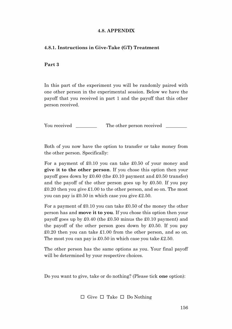
156

4.8. APPENDIX

4.8.1. Instructions in Give-Take (GT) Treatment

Part 3

In this part of the experiment you will be randomly paired with

one other person in the experimental session. Below we have the

payoff that you received in part 1 and the payoff that this other

person received.

You received _________ The other person received _________

Both of you now have the option to transfer or take money from

the other person. Specifically:

For a payment of £0.10 you can take £0.50 of your money and

give it to the other person. If you chose this option then your

payoff goes down by £0.60 (the £0.10 payment and £0.50 transfer)

and the payoff of the other person goes up by £0.50. If you pay

£0.20 then you give £1.00 to the other person, and so on. The most

you can pay is £0.50 in which case you give £2.50.

For a payment of £0.10 you can take £0.50 of the money the other

person has and move it to you. If you chose this option then your

payoff goes up by £0.40 (the £0.50 minus the £0.10 payment) and

the payoff of the other person goes down by £0.50. If you pay

£0.20 then you can take £1.00 from the other person, and so on.

The most you can pay is £0.50 in which case you take £2.50.

The other person has the same options as you. Your final payoff

will be determined by your respective choices.

Do you want to give, take or do nothing? (Please tick one option):

Give Take Do Nothing

157

If you chose Give/Take, then how much do you want to

Give/Take? (Please tick one option):

£0.00 £0.50 £1.00 £1.50 £2.00 £2.50

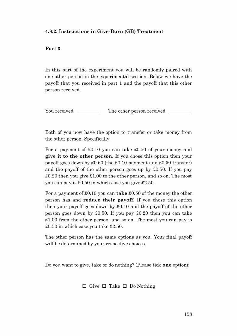
158

4.8.2. Instructions in Give-Burn (GB) Treatment

Part 3




person received.











person has and reduce their payoff. If you chose this option

then your payoff goes down by £0.10 and the payoff of the other

person goes down by £0.50. If you pay £0.20 then you can take

£1.00 from the other person, and so on. The most you can pay is

£0.50 in which case you take £2.50.



Do you want to give, take or do nothing? (Please tick one option):

Give Take Do Nothing

159



£0.00 £0.50 £1.00 £1.50 £2.00 £2.50

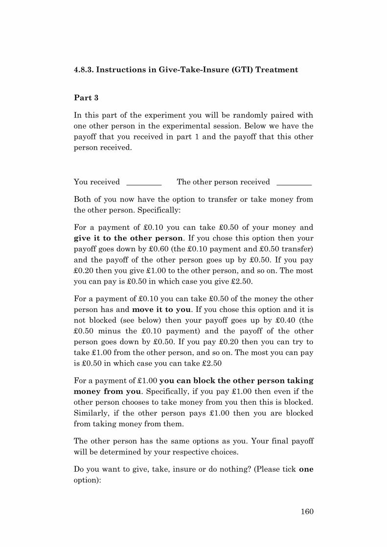
160

4.8.3. Instructions in Give-Take-Insure (GTI) Treatment

Part 3




person received.











person has and move it to you. If you chose this option and it is

not blocked (see below) then your payoff goes up by £0.40 (the

£0.50 minus the £0.10 payment) and the payoff of the other

person goes down by £0.50. If you pay £0.20 then you can try to

take £1.00 from the other person, and so on. The most you can pay

is £0.50 in which case you can take £2.50

For a payment of £1.00 you can block the other person taking

money from you. Specifically, if you pay £1.00 then even if the

other person chooses to take money from you then this is blocked.

Similarly, if the other person pays £1.00 then you are blocked

from taking money from them.



Do you want to give, take, insure or do nothing? (Please tick one

option):

161




£0.00 £0.50 £1.00 £1.50 £2.00 £2.50

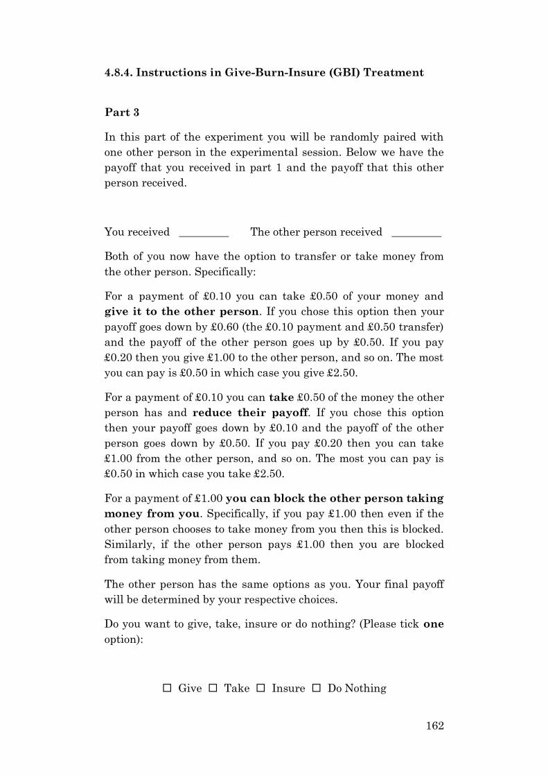
162

4.8.4. Instructions in Give-Burn-Insure (GBI) Treatment

Part 3




person received.











person has and reduce their payoff. If you chose this option

then your payoff goes down by £0.10 and the payoff of the other

person goes down by £0.50. If you pay £0.20 then you can take

£1.00 from the other person, and so on. The most you can pay is

£0.50 in which case you take £2.50.

For a payment of £1.00 you can block the other person taking

money from you. Specifically, if you pay £1.00 then even if the

other person chooses to take money from you then this is blocked.

Similarly, if the other person pays £1.00 then you are blocked

from taking money from them.



Do you want to give, take, insure or do nothing? (Please tick one

option):


163



£0.00 £0.50 £1.00 £1.50 £2.00 £2.50

164

4.8.5. Post-Experiment Questionnaire

For the final part of this experiment, please answer the following

questions to the best of your knowledge.

1. Gender

Male

Female

2. Religious Affiliation

Christian (Protestant)

Christian (Catholic)

Hindu

Jewish

Sikh

Muslim

Atheist

Agnostic

Buddhist

Other

3. Ethical or moral issues do not

influence where or how I decide to

spend my money:

Strongly Agree

Agree

Neither Agree nor Disagree

Disagree

Strongly Disagree

4. When I am faced with a financial

decision, I am generally more

concerned about the possible losses

than probable gains.

Strongly Agree

Agree


Disagree

Strongly Disagree

5. I feel it is justified to do anything I

can get away with in order to succeed.

Strongly Agree

Agree


Disagree

Strongly Disagree

6. It is morally justifiable to hurt others

in pursuit of my own goals.

Strongly Agree

Agree


Disagree

Strongly Disagree

7. It is morally justifiable to steal from

others in pursuit of my own goals.

Strongly Agree

Agree


Disagree

Strongly Disagree

8. Exploiting others to achieve success

and improve one’s social situation is

justifiable.

Strongly Agree

Agree


Disagree

Strongly Disagree

9. Cheating isn’t justified because it is

unfair to others.

165

Strongly Agree

Agree


Disagree

Strongly Disagree

10. Whether cheating is judged to be

moral or immoral depends upon the

circumstances surrounding the

action.

Strongly Agree

Agree


Disagree

Strongly Disagree

11. In Part 2 of the experiment, did you

expect the other person to:

A. Give

B. Take

12. Which of the following objectives is

most important for you?

Maximizing my own outcomes

regardless of others.

Maximizing my own outcomes

relative to others.

Maximizing joint outcomes.

13. In Part 2 of the experiment, I was

worried about the possibility of the

other person taking my money.

Strongly Agree

Agree


Disagree

Strongly Disagree

14. In Part 2 of the experiment, I felt

envious towards the other person.

Strongly Agree

Agree


Disagree

Strongly Disagree

15. If given the option, I would be willing

to pay to reduce someone else’s

income out of spite/envy.

Strongly Agree

Agree


Disagree

Strongly Disagree

16. If income inequality reflected

differences in effort as opposed to

luck or privilege, this would affect my

willingness to redistribute or donate

money.

Strongly Agree

Agree


Disagree

Strongly Disagree

17. If given the option, I would be willing

to pay to reduce someone else’s

income for issues relating to fairness.

Strongly Agree

Agree


Disagree

Strongly Disagree

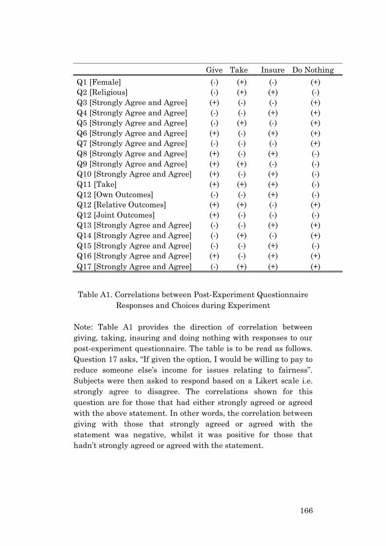
166


Q1 [Female] (-) (+) (-) (+)

Q2 [Religious] (-) (+) (+) (-)

Q3 [Strongly Agree and Agree] (+) (-) (-) (+)

Q4 [Strongly Agree and Agree] (-) (-) (+) (+)

Q5 [Strongly Agree and Agree] (-) (+) (-) (+)

Q6 [Strongly Agree and Agree] (+) (-) (+) (+)

Q7 [Strongly Agree and Agree] (-) (-) (-) (+)

Q8 [Strongly Agree and Agree] (+) (-) (+) (-)

Q9 [Strongly Agree and Agree] (+) (+) (-) (-)

Q10 [Strongly Agree and Agree] (+) (-) (+) (-)

Q11 [Take] (+) (+) (+) (-)

Q12 [Own Outcomes] (-) (-) (+) (-)

Q12 [Relative Outcomes] (+) (+) (-) (+)

Q12 [Joint Outcomes] (+) (-) (-) (-)

Q13 [Strongly Agree and Agree] (-) (-) (+) (+)

Q14 [Strongly Agree and Agree] (-) (+) (-) (+)

Q15 [Strongly Agree and Agree] (-) (-) (+) (-)

Q16 [Strongly Agree and Agree] (+) (-) (+) (+)

Q17 [Strongly Agree and Agree] (-) (+) (+) (+)

Table A1. Correlations between Post-Experiment Questionnaire

Responses and Choices during Experiment

Note: Table A1 provides the direction of correlation between

giving, taking, insuring and doing nothing with responses to our

post-experiment questionnaire. The table is to be read as follows.

Question 17 asks, “If given the option, I would be willing to pay to

reduce someone else’s income for issues relating to fairness”.

Subjects were then asked to respond based on a Likert scale i.e.

strongly agree to disagree. The correlations shown for this

question are for those that had either strongly agreed or agreed

with the above statement. In other words, the correlation between

giving with those that strongly agreed or agreed with the

statement was negative, whilst it was positive for those that

hadn’t strongly agreed or agreed with the statement.

167

CHAPTER FIVE

5. CONCLUSION

This thesis covered three independent research questions.

Chapter two argued that the regulatory constraints imposed by

the Shariah on Islamic securities and investors, such as the

prohibition of trade in derivative contracts, impedes the ability of

Islamic portfolio managers to utilise important risk-management

strategies. In light of this, chapter two studied a) whether

diversifying across asset-classes by including commodities and

Sukuk (Islamic Bonds) could improve the performance of an

equity-only Islamic portfolio b) the benefits of diversification over



dynamic conditional correlation between the aforementioned

asset-classes to study how the relationship across markets is

affected during crisis regimes and d) given that Islamic portfolios

are vulnerable to extreme events, I employed a convenient tail-

risk measure of performance which includes the importance of an

assets skewness and kurtosis to study whether taking into

account the shape of the returns’ distribution provides further

insight into the potential benefits of diversification.

The results from chapter two showed that in terms of improving

risk-return profiles, the benefit of diversifying beyond an equity-

only portfolio is limited during normal times but advantageous

during crisis periods. The most important finding from chapter

two relates to the estimation of portfolio tail-risk. In particular, I

demonstrated that using a standard two-moment Value-at-Risk

measure, which assumes normally distributed returns, rather

than a four-moment Value-at-Risk measure, which incorporates

an assets skewness and kurtosis, can lead to a substantial


conditions.

The aforementioned results have important practical implications

for portfolio managers and practitioners within the Islamic

Finance sector. As argued in chapter two, Shariah-compliant

168

securities are likely to deviate from a normal distribution as well

as being vulnerable to extreme shocks for reasons such as market

thinness, shortages of liquidity, the lack of product

standardisation, underdeveloped secondary markets and the

inability to diversify across a more comprehensive range of

market sectors. Hence, our results provide important insights into

the benefits of asset-class diversification and highlight the

importance of taking into consideration a more complete

description of the distribution of returns.

Given the distinctive characteristics and requirements of Shariah-

compliant assets, an interesting avenue for future research, which

has so far received little attention, is the study and development

of risk-factor models specific to Shariah-based securities. With the

growing relevance of assets such as Sukuk, it has become

increasingly important to determine the risk-factors and relative

importance of market and institutional factors in influencing the

prices of niche Islamic securities. Such research could further

support practitioners in improving the management of risk in

their portfolios.

In chapter three, we explored the extent to which elicited

measures of risk-aversion are influenced by religious priming and

the way in which the decision-task is framed. Using the seminal

Gneezy and Potters (1997) framework, we found that risk-taking

is significantly higher when an identical task is framed in terms

of an investment rather than a gamble. Furthermore, our results

suggest that using a religious prime or setting (a Mosque)

significantly lowers risk-taking in the gambling frame whilst

having no effect in the investment frame. The elicited measures of

risk-aversion were influenced by a range of factors including

gender, ethical standards and setting in the gambling frame

whereas we observed no such effect in the investment frame. We

argue that this sensitivity towards a gambling frame is due to

social and religious norms around gambling. This is an important

result as it suggests that risk-preference elicitation tasks that are

framed in terms of gambling, as many are, likely lead to

systematic bias. Hence, an important implication derived from

our experiments in chapter three is that we should look to test

and develop methods of measuring risk-preferences that avoid a

gambling frame. Overall, our findings corroborate the results of

previous studies that show the fundamental importance of context

169

in determining individual risk-taking (Weber 2012, Dohmen et al.

2011, Schubert et al. 1999).

Chapter four presented the results from a simple incentivised

laboratory experiment that tested whether altering subject choice-

sets influences the level of prosociality. Subsequent to an effort-

stage where subjects competed in a winner-takes-all tournament

to earn their endowment, subjects had the opportunity to do

nothing, give or take money from their opponent or in the

insurance treatment, insure. We additionally tested for any

differences in the observed behaviour of subjects when any

amount stolen from their opponent was kept versus when it was

burned (wasted).

We report several interesting findings. First, consistent with

previous studies, we find strong evidence of agents displaying

both positive and negative other-regarding preferences, which

contradicts the model of narrow self-interest (e.g. Zizzo and

Oswald (2001), Andreoni et al. (2007), Abbink and Sadrieh (2009)

and Engel (2011)). Second, we observe that the behaviour of

subjects can be sensitive to changes in the choice-set they are

presented with, even when the options added onto the choice-set

constitute monetarily dominated strategies. Moreover, our results

suggest that altering choice-sets had an asymmetric effect on the

attitudes of competition winners and losers. Particularly,

expanding the available choice-set to include the option of

insurance crowded out donations from competition winners and

shifting from the take-and-keep to take-and-burn treatment

lowered the average size of donations. In contrast, neither the

expansion of the choice-set nor the switch from the take-and-keep

treatment to the take-and-burn treatment had any impact on

stealing by competition losers. This was both in terms of the

fraction of subjects that decided to steal and the size of the

amounts stolen. Hence, we found that the aforementioned

changes to the decision-task were more effective at lowering

prosocial behaviour by competition winners whilst being less

effective at having any impact on the antisocial behaviour of

competition losers.

Similar to chapter three, the results from chapter four corroborate

the findings from previous studies showing that behaviour can be

sensitive to changes in the exact context and choice-set presented

to subjects (List (2007), Bardsley (2008) and Dohmen et al.

170

(2011)). More broadly, in combination with the prior literature, an

important overarching implication of our findings from chapters

three and four is that the situational instability of preferences

observed in the lab is likely responsible for the lack of external

validity of experimental studies. While the experimental

literature has provided valuable insights through theory-testing,

in order to address concrete real-world problems there is a need

for greater emphasis on context-specific studies, the results of

which may only have limited scope in terms of generalizability

(see Guala and Mittone 2005).

Documents

85PhD (OS).pdf - Kent Academic Repository