A comparison of some parallel game-tree search algorithms (Revised version)

A comparison of some parallel game-tree search algorithms(Revised version)

Jaleh Rezaie ([email protected])Raphael Finkel ([email protected])

Department of Computer ScienceUniversity of Kentucky

Lexington, KY 40506-0027

AbstractThis paper experimentally compares several sequential and parallel game-tree

search methods: alpha-beta, mandatory work first, principal-variation splitting, tree split-ting, ER, and delay splitting. All have been implemented in a common environment pro-vided by the DIB package.

Key words: game trees, heuristic search, alpha-beta

1. IntroductionIn this paper we compare some of the parallel methods for searching large game

trees. These trees arise in the area of artificial intelligence and are closely related to treessearched in other application areas. Exhaustive search of a tree is prohibitively expen-sive. There are several ways to ameliorate the problem.

g Search only to a given depth.g Apply heuristics, such as the alpha-beta method, to cut off fruitless search.g Apply many computers simultaneously in pursuing the search.

We concentrate on distributed variants of the alpha-beta heuristic that try to avoid search-ing unnecessary parts of the tree while keeping many processors fruitfully busy.

The algorithms we compare are alpha-beta, mandatory work first, principal-variation splitting, tree splitting, ER, and delay splitting. To be able to make a fair com-parison between the above algorithms, we have extended the DIB package [1] to use it asa framework for implementing all the algorithms we compare.

Section 2 describes the DIB package. Section 3 introduces the alpha-beta pruningand briefly describes the algorithms used in the experiment. Section 4 presents experi-mental results that compare the algorithms. Section 5 compares the effects of severalsorting strategies on the above algorithms. Section 6 illustrates the new results achievedby adjustments made to MWF algorithm. Section 7 summarizes the results, and detailsremaining parts of this experiment.

2. DIB — A distributed implementation of backtrack-ing

In this section we describe how DIB works and how we use it to implement dif-ferent tree-search algorithms.

Game-tree search 2

2.1. Description of DIBDIB is a multi-purpose package developed by Finkel and Manber for tree-traversal

problems [1]. It allows applications such as backtrack and branch-and-bound to beimplemented on a multicomputer. DIB’s requirements from the distributed operatingsystem are minimal. The machines must be connected by a network that supports amessage-passing mechanism; each machine must be able to communicate, not neces-sarily directly, with all other machines. Our implementation of DIB is programmed in Cand runs in the Unix environment across machines connected by an internet or on a Unixmultiprocessor.

The application program must specify the root of the problem tree, how to generatechildren, and calculations needed at each node. It can also optionally specify how togenerate values of a tree node from combining its children’s values and how to spreadinformation either globally or locally throughout the tree.

DIB divides the problem into subproblems and assigns them to any number of pro-cessors (potentially nonhomogeneous machines in a network) dynamically. Each proces-sor maintains a table of explicit work, recording all the problems that have been sent tothe processor, have been generated by the processor itself, and/or have been sent to otherprocessors. Each processor is responsible for the work in its table. Each item of work(represented by a node in the backtrack tree, which stands as well for all its descendents)is labeled by which processor, if any, has been assigned that work.

When a processor A is finished with a problem and has reported its result to the pro-cessor that gave it that problem, it will take the first (in an inorder traversal of the tree)unassigned problem from its table. If no unassigned problem is available, A sends awork request message to another processor (or processors), selected at random from A ’speers, repeatedly (with some delay) until new work arrives.

A processor B that receives a work request message interrupts its own search andtrys to respond by sending some work to the requesting processor from its table. If nounassigned problem is available in the table, then the problem B is working on is subdi-vided and its children are put in the table. Until work is subdivided, DIB maintains a fastrepresentation of the current search (just a recursion stack; we call it the ‘‘implicit’’representation); subdivided work is explicit in the table. After subdivision, B can usuallysend some unassigned work to the requesting processor. Subdivision may have to berepeated several times before an unassigned problem is generated, but if it reaches atrivial problem (not worth subdividing), or if it reaches the depth at which B itself issearching, the request is not granted. B resumes its search after dealing with the incom-ing request.

DIB is fault tolerant, in that work that B has given to A can still be accomplishedby B if there is nothing else worth doing and if A has not yet reported the result of thatwork. This mechanism does not need timeouts or ‘‘heartbeats’’ to detect failure.

We have enhanced the DIB package so that it can achieve high efficiency for gametree search. The principal enhancement is added flexibility given to the application levelfor delaying evaluation of a game-tree node. That is, the application can refuse to gen-erate additional children for a node but indicate that in the future it may again be willingto do so. DIB does not attempt to generate children of such a node again until someother child of that node has completed or a data update message has arrived at that node.

Game-tree search 3

To experiment with game playing, we have designed a two-level application struc-ture. The game level is game-specific, knowing the rules for tic-tac-toe, Othello, orcheckers. The control level communicates both with DIB and the game level. It knowsthe pattern of evaluation for one of the algorithms we compared, namely, alpha-beta,mandatory work first, principal-variation splitting, tree splitting, ER, or delay splitting.Any of the game modules we implemented can be used with any of the control modules;any such combination can be used with our enhanced DIB.

Since DIB distributes work, collects and reports results, and passes messagesbetween processors in a similar way for all the combinations, we can compare differentcontrol modules in a fairly implementation-independent fashion. Previous comparisonsare questionable because each algorithm was implemented in a different parallel environ-ment.

3. Parallel tree search algorithmsThe best way to evaluate a parallel algorithm for a given problem is to measure the

extent in which it takes advantage of available processors. This idea can be formulatedas follows:

speedup S =time required by parallel algorithm

time required by best sequential algorithmhhhhhhhhhhhhhhhhhhhhhhhhhhhhhhhhhhhhh

efficiency E =number of processors used

Shhhhhhhhhhhhhhhhhhhhhhhh

It is not easy to achieve a ‘‘perfect’’ efficiency of 1.0. For a given sized problem,efficiency tends to decrease as the number of processors increases. This relationship isexplained by Kumar and Rao [2] as resulting from an increase in the communication time(sum of the time spent by all processors in communicating with neighboring processors,waiting for messages, time in starvation, and so forth), while there is no change in com-putation time (sum of the time spent by all the processors in useful computation). Therelationship between communication time (Tcm ), computation time (Tcp ), and efficiency(E) is described as follows:

E =Tcp +Tcm

Tcphhhhhhhh

Kumar and Rao [2] define an isoefficiency function that shows how the problemmust grow with number of processors to achieve the same efficiency. They also mentionthat since most problems have a sequential component (in depth-first search, it is onenode expansion), problem size must grow at least linearly to maintain a particularefficiency.

Steinberg and Solomon [3] blame the failure to achieve perfect efficiency on threetypes of ‘‘loss’’.

g Starvation loss: processors sitting idle while awaiting work to be given to them.g Interference loss: time spent waiting for access to shared resources such as the set of

unfinished subproblems.g Speculative loss: time spent performing unnecessary work, such as that performed by

a parallel algorithm before it is possible to determine that the work is necessary.

Game-tree search 4

Because a parallel algorithm must evaluate different nodes simultaneously, informa-tion gained by evaluation of one node could come too late to cut off evaluation ofother nodes.

3.1. Alpha-betaThe alpha-beta algorithm is a sequential technique used to evaluate a game tree

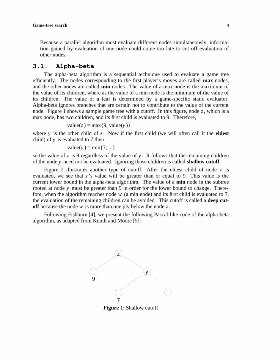
efficiently. The nodes corresponding to the first player’s moves are called max nodes,and the other nodes are called min nodes. The value of a max node is the maximum ofthe value of its children, where as the value of a min node is the minimum of the value ofits children. The value of a leaf is determined by a game-specific static evaluator.Alpha-beta ignores branches that are certain not to contribute to the value of the currentnode. Figure 1 shows a sample game tree with a cutoff. In this figure, node z , which is amax node, has two children, and its first child is evaluated to 9. Therefore,

value(z ) = max{9, value(y )}

where y is the other child of z . Now if the first child (we will often call it the eldestchild) of y is evaluated to 7 then

value(y ) = min{7, ...}

so the value of z is 9 regardless of the value of y . It follows that the remaining childrenof the node y need not be evaluated. Ignoring those children is called shallow cutoff.

Figure 2 illustrates another type of cutoff. After the eldest child of node z isevaluated, we see that z ’s value will be greater than or equal to 9. This value is thecurrent lower bound in the alpha-beta algorithm. The value of a min node in the subtreerooted at node y must be greater than 9 in order for the lower bound to change. There-fore, when the algorithm reaches node w (a min node) and its first child is evaluated to 7,the evaluation of the remaining children can be avoided. This cutoff is called a deep cut-off because the node w is more than one ply below the node z .

Following Fishburn [4], we present the following Pascal-like code of the alpha-betaalgorithm, as adapted from Knuth and Moore [5]:

z

y9

7Figure 1: Shallow cutoff

Game-tree search 5

z

y

x

w

9

7Figure 2: Deep cutoff

function alphabeta(z : position; α, β : integer):integer;var

Answer, Child, t, d : integer;begin

determine the child positions z 1,..., zdif d = 0 then

return(StaticValue(z))else

beginAnswer := α ;for Child := 1 to d do

begint := -alphabeta(zChild , -β, -Answer);if t > Answer then

Answer := t;if Answer ≥ β then

return(Answer); {cutoff}end;

return(Answer);end;

end.

The alpha-beta algorithm satisfies the following conditions [5]:

if negamax(z ) ≤ α then alphabeta(z , α, β) ≤ α,if α < negamax(z ) < β then alphabeta(z , α, β) = negamax(z ),if negamax(z ) ≥ β then alphabeta(z , α , β) ≥ β.

These conditions imply that

Game-tree search 6

alphabeta(z , −∞, ∞) = negamax(z ) ,

which means that if the initial window [alpha, beta] is (−∞, ∞) then the alpha-beta algo-rithm returns the same value as the negamax algorithm (straightforward tree-evaluationalgorithm that never cuts work off) [5].

The performance of the alpha-beta algorithm depends a great deal on the order inwhich children of a node are expanded. If the children of each node in the game tree areexpanded in increasing order of their negamax values, then the largest number of cutoffswill occur.

Knuth and Moore [5] introduced the idea of critical nodes in their analysis of thebest case of the alpha-beta algorithm, and Steinberg and Solomon [3] use the followingrules to determine the critical nodes:

g The root of the game tree is a type-1 node.g The eldest child of a type-1 node is also type-1. The remaining children are type-2.g The eldest child of a type-2 node is a type-3 node.g All children of a type-3 node are type-2.g A node is critical iff it is assigned a number by the above rules.

The critical nodes form a minimal subtree [3] of the game tree which, regardless ofthe values of the terminal nodes, will always be examined by the alpha-beta algo-rithm [5]. The number of terminal nodes in the minimal subtree of a complete d-ary treeof height h is

d Rh /2 H+d Qh /2 P−1

If the tree is examined in increasing order of value, the alpha-beta procedure examinesprecisely the minimal subtree of the game tree. In short, alpha-beta examines about 2n 1/2

nodes, where negamax would examine n nodes.

3.2. Mandatory work first (MWF)This algorithm was proposed by Akl, Barnard, and Doran as a parallel implementa-

tion of alpha-beta without deep cutoffs. The name MWF was coined by Fishburn andFinkel. MWF evaluates critical nodes concurrently and then returns to evaluate othernodes if needed [6, 7]. When deep cutoffs are not considered in the search algorithm,only type-1 and type-2 nodes are critical, as shown in Figure 3.

MWF evaluates type-1 nodes completely, but only evaluates type-2 nodes partially.After the eldest child of a type-1 node (also type-1) has been evaluated, the remainingchildren (all type-2) are completely evaluated only if the result of the partial evaluation isnot sufficient to cut them off. All evaluations currently allowed by MWF may be under-taken simultaneously.

Akl, Barnard, and Doran [6] tested MWF with game trees of depth 4 and branchingfactors of 5, 10, 15 and 20. They noticed that MWF has a better efficiency when thegame tree has a larger fanout, but found that the speedup reaches a plateau around six.The total number of nodes visited as well as the number of terminal nodes examinedshowed an increase with increasing number of processors, but the plateau was reachedmuch faster.

Fishburn [4] analyzed MWF for best-first and worst-first ordering of the game tree.In the best-first ordering, MWF is almost optimal, since its efficiency is very close to 1

Game-tree search 7

1

1

1

1 1 1

1 1

1

2 2

2 2

2 2 2 2 2 21

Figure 3: Minimal subtree when deep cutoffs are not considered

when a large number of processors is used. For the worst-first ordering, Fishburn used anexample game tree of degree 38 and processor tree of fanout 2 to predict that speedup forMWF will satisfy

p 0.93 ≤ S ≤ p 0.96

where p is the number of processors. This result is almost as good as tree-splitting.

3.3. The tree-splitting algorithmFishburn proposed this method as a natural parallel way to implement the alpha-

beta algorithm. The tree-splitting algorithm splits the game tree into its subtrees at theroot node, and each subtree is assigned to a pool of processors for evaluation [4]. Thepool will evaluate the subtree in parallel if it has more than one processor. In otherwords, the game tree is mapped to a processor tree. as shown in Figure 4. Here we havea binary tree of processors with height two (connected by heavy arcs) mapped onto a ter-nary game tree. When there are more branches in the game tree than there are in the pro-cessor tree, the extra game tree branches are queued and assigned to a processor whenone becomes available.

All interior processors in the tree of processors are both masters and slaves exceptthe root processor, which is only a master. All the leaf processors are slaves. When aslave processor finishes the search of its assigned subtree, it reports the value computedto its master. When a master processor receives a response from one of its slaves, itupdates its alpha-beta window and informs the other working slaves of this new window.The new window may allow the remaining work under the master to be cutoff. When allthe slaves have finished, either by cutoff or by reporting their values, the master proces-sor can compute the value of its own position.

Fishburn [4] calculates the speedup for the tree-splitting algorithm for two differentorderings of the game tree. Worst-first ordering produces no alpha-beta cutoffs. It isachieved by sorting all children of all nodes so that whenever the call alphabeta(z , α, β)

Game-tree search 8

Figure 4: Processor tree mapped onto game tree

is made, the following relation holds among the children z 1 ,..., zd :

α < −negamax(z 1) <... < −negamax(zd ) < β

Since there are no cutoffs, there is no speculative loss, so tree splitting achieves practi-cally perfect speedup.

Best-first ordering produces the maximum number of alpha-beta cutoffs. It isachieved by sorting all children of all nodes so that:

negamax(z ) = −negamax(z 1) for all nodes z in the game tree.

Using this ordering, the tree-splitting algorithm gives S = O(p 1/2) with p processors.

The tree-splitting algorithm gives S = O(p 1/2) with p processors when best-first ord-ering [4] of the game tree is used.

3.4. Principal-variation (PV) splittingPV splitting is a refinement of the tree-splitting algorithm [8]. It assumes that the

search tree is mapped onto an underlying tree of processors and that the game tree isstrongly ordered, that is, the first branch of each node is the best branch at least 70 per-cent of the time and that the best move is in the first quarter of the branches beingsearched 90 percent of the time.

The type-1 nodes are recursively evaluated until a given ply is reached, at whichpoint tree splitting is used. After the value of the principal variation (type-1) node isbacked up the tree, tree splitting is used to evaluate the remaining siblings if they can notbe cut off.

There are two differences between PV splitting and MWF. First, PV splittingrequires a particular underlying processor structure, in contrast with the pool of proces-sors used in MWF. Second, it waits for the search of type-1 nodes to end before it startsevaluating the other nodes. This aspect of PV splitting ensures that the best availablevalue of α is passed to the other nodes of the tree.

Game-tree search 9

PV splitting was compared experimentally with the tree splitting algorithm usingtrees of depth 4 and width 24. Experimental results show that PV splitting outperformstree splitting, especially when a wider processor tree is used [8]. For example, when aprocessor tree with both depth and width of 2 was used, tree-splitting examined 912nodes, and PV splitting examined 648 nodes. But when the width of the processor treewas changed to 8, tree-splitting and PV splitting examined 772 and 277 nodes respec-tively.

3.5. The ER algorithmThis algorithm was developed by Steinberg and Solomon for parallel evaluation of

game trees. It is a sequential algorithm with a parallel implementation [3]. The nodes inthe game tree are divided into two groups, e-nodes and r-nodes. E-nodes will be fullyevaluated, and r-nodes will be refuted, that is, will have an estimated value. All childrenof an e-node are evaluated, but as few as one child of an r-node needs to be examined.Therefore e-nodes are more ‘‘costly’’ than r-nodes. Every internal node has exactly onee-node child (e-child).

Any child of a node can be chosen as the e-child, but the child with the lowestnegamax value is the best choice [3].

To choose the e-child of a node z , ER evaluates the elder grandchildren (eldest chil-dren of z ’s children) in parallel, and chooses the child whose elder child has the largestvalue. The e-child is then evaluated while avoiding re-evaluation of its oldest child,since we just got its value. The remaining children are refuted in order.

In the parallel implementation of ER, the elder grandchildren can be evaluated inparallel because they represent mandatory work. Since these grandchildren are them-selves e-nodes, their elder grandchildren can also be recursively evaluated in parallel.These parallel evaluations are mandatory work, but if ER is to perform only the manda-tory work, the remaining siblings of an e-node must be examined sequentially. To avoidthese sequential evaluations and thus starvation loss, ER uses the following two methods:

g Parallel refutation: After an e-child y of an e-node z is evaluated, refute y ’s siblingsin parallel. This parallel evaluation is likely to encounter lots of speculative loss.This work is similar to the speculative work performed by MWF and PV splittingalgorithms.

g Multiple e-children: After an e-child of an e-node z is evaluated, choose the next bestchild of z as a second e-child. If it happens that the first e-child is not actually thebest child of z (other children cannot be immediately refuted), we will have anothere-child that will hopefully help us cut off z ’s other children. In general, after the firste-child has been evaluated, ensure that z always has one active e-child.

Steinberg and Solomon compared ER to PV splitting. Sequential ER evaluatesmore nodes than alpha-beta, but sequential PV splitting is identical to alpha-beta. Forthis reason Steinberg and Solomon [3] used relative efficiency and relative speedup asshown below to compare the two algorithms.

relative efficiency =no. of processors used

relative speeduphhhhhhhhhhhhhhhhhhhh

Game-tree search 10

relative speedup =time required by parallel algorithm

time required by parallel algorithm with 1 processorhhhhhhhhhhhhhhhhhhhhhhhhhhhhhhhhhhhhhhhhhhhhh

Experiments show that ER achieves twice the efficiency and speedup of the PV splittingalgorithm when used on sufficiently deep trees [3]. The average efficiency achieved byER using 16 processors for 7, 8, 9, and 10 ply trees are respectively 0.44, 0.52, 0.68, and0.58. The corresponding efficiencies for PV splitting are 0.28, 0.31, 0.31, and 0.31. Therange of speedup for 7 to 9 ply trees using 16 processors are 7.1 to 10.9 for the ER algo-rithm and 4.5 to 5.0 for the PV splitting algorithm. Steinberg and Solomon contributeER’s higher efficiency to low starvation loss.

3.6. Delay splittingThis algorithm delays the evaluation of each node until its eldest sibling is com-

pletely evaluated. Starvation loss is accepted in order to increase the number of cutoffs.Evaluation delay occurs at every level for each node, thus making delay splitting dif-ferent from PV splitting, in which delay of evaluation occurs only along the principlevariation route.

The following is Pascal-like code for delay splitting:function DelaySplit(z : position; α, β): integer;

var d, i : integer;value : array[1..MAXWIDTH] of integer;

beginif (I am a leaf processor) then

return(alphabeta(z, α, β));determine the child positions z 1, ..., zdα = -DelaySplit(z 1, −β, −α);if α ≥ β then

return(α);for i := 2 to d do in parallel

beginvalue[i] := -DelaySplit(zi , −β, −α);begincrit {critical region }

if value[i] > α thenα := value[i];

endcrit;if α ≥ β then

return(α); { cutoff }end;

end. { DelaySplit }

4. Experimental resultsWe have tested the above algorithms on a Sequent Symmetry with 26 cpus using an

unsorted tree of depth 9 and fanout of at most 15 (the fanout decreases by one at eachlevel) generated by the game tic-tac-toe. The algorithms tend to have more cutoffs witha sorted tree, but are likely to have a higher efficiency with a worst-first sorted tree. Notsorting at all gives us a comparison with a reasonable amount of cutoff and a reasonableamount of parallelism. The relative efficiency comparisons are shown in Figure 5.(Relative efficiency compares the parallel execution time to the sequential execution timeof the same algorithm in the same environment. The sequential execution times of allalgorithms we tested are quite similar.) For this particular test, the MWF algorithm

Game-tree search 11

achieved an almost perfect efficiency, followed by delay splitting and ER algorithmswith speedup of over 12 and 9 respectively, using 20 processors. We attribute our abilityto exceed a speedup of 6 with MWF to DIB’s parallelization environment and the treestructure used in this experiment.

Figure 6 shows the ratio of the number of nodes examined by the algorithms usingdifferent numbers of machines verses using one machine (sequential algorithm).

alphabeta

MWF

delaysplit

TreeSplit10

ER

PVS10

1 3 5 7 9 11 13 15 17 19 210.00

0.10

0.20

0.30

0.40

0.50

0.60

0.70

0.80

0.90

1.00

Figure 5: Efficiency vs number of machines

Game-tree search 12

alphabeta

delaysplit

TreeSplit10PVS10

MWF

ER

1 3 5 7 9 11 13 15 17 19 21 23

0.00

1.00

2.00

3.00

Figure 6: Relative no. of nodes examined vs. number of machines

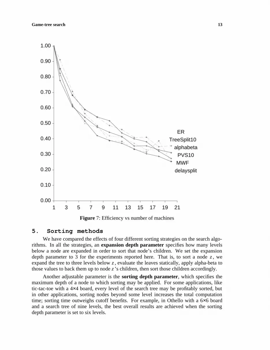
We have also tested the algorithms using Othello with a 6×6 board. All algorithmshave almost the same relative efficiency, with delay splitting leading when fewer than sixprocessors are used. In this experiment, the speedup did not exceed 7 (Figure 7).

Game-tree search 13

alphabeta

MWF

delaysplit

TreeSplit10

ER

PVS10

1 3 5 7 9 11 13 15 17 19 210.00

0.10

0.20

0.30

0.40

0.50

0.60

0.70

0.80

0.90

1.00


5. Sorting methodsWe have compared the effects of four different sorting strategies on the search algo-

rithms. In all the strategies, an expansion depth parameter specifies how many levelsbelow a node are expanded in order to sort that node’s children. We set the expansiondepth parameter to 3 for the experiments reported here. That is, to sort a node z , weexpand the tree to three levels below z , evaluate the leaves statically, apply alpha-beta tothose values to back them up to node z ’s children, then sort those children accordingly.

Another adjustable parameter is the sorting depth parameter, which specifies themaximum depth of a node to which sorting may be applied. For some applications, liketic-tac-toe with a 4×4 board, every level of the search tree may be profitably sorted, butin other applications, sorting nodes beyond some level increases the total computationtime; sorting time outweighs cutoff benefits. For example, in Othello with a 6×6 boardand a search tree of nine levels, the best overall results are achieved when the sortingdepth parameter is set to six levels.

Game-tree search 14

Our first attempt at sorting was to sort only the children of the top node. Thisregime, called ‘‘TN (top-node) sorting’’, applies to all the algorithms except ER, whichhas its own internal sorting mechanism. There is no noticeable difference in number ofnodes, total time, or efficiency for any of the algorithms between TN and no sorting atall.

Next we extended the sorting to include all nodes on the principal variation route.We call this sorting regime ‘‘PVR sorting’’. Our tests of PVR sorting for PV spitting,MWF, and delay splitting show no significant improvement in total computation time.

In the third sorting regime, we sort at the top node and at every eldest child. Wecall this sorting regime ‘‘EC (eldest child) sorting’’. EC sorting applies to MWF anddelay splitting, since only in these two algorithms do we suspend evaluation of all nodesthat are not eldest children until their eldest sibling is fully evaluated. Therefore havingthe best child evaluated first should result in more cutoffs.

As expected, the results are much better for EC sorting than PRV sorting, as evi-denced by tests with our tic-tac-toe and Othello applications. The total computation timeis almost reduced by half when fewer machines are used. The reduction in the efficiency,expected due to the improvement in the sequential performance of the algorithms, is nottoo bad. Figures 8, 9 and 10 show the number of nodes examined (in multiples of 1000),total time and efficiency comparisons for MWF using the 4×4 tic-tac-toe game.

MWF(EC-sorting)

MWF(NoSorting)

1 3 5 7 9 11 13 15 17 19 210.00

50.00

100.00

150.00

200.00

250.00

300.00

350.00

400.00

450.00

500.00

550.00

600.00

650.00

Figure 8: Nodes examined vs. number of machines

Game-tree search 15

MWF(NoSorting)

MWF(EC-sorting)

SortTime(EC-sorting)

1 3 5 7 9 11 13 15 17 19 210.00

40.00

80.00

120.00

160.00

200.00

240.00

280.00

320.00

360.00

400.00

Figure 9: Time vs. number of machines

MWF(EC-sorting)

MWF(NoSorting)

1 3 5 7 9 11 13 15 17 19 210.00

0.10

0.20

0.30

0.40

0.50

0.60

0.70

0.80

0.90

1.00

Figure 10: Efficiency vs. number of machines

Game-tree search 16

The last sorting regime is motivated by considering the type-2 nodes in MWF. Theeldest child of a type-2 node is evaluated before its other children are generated. There-fore, if we also sort the children of a type-2 node there should be even more cutoffs. Inthis sorting regime, in addition to sorting children of every eldest child, we also sort atevery type-2 node. We call this regime ‘‘TT (type-two) sorting’’.

TT sorting resulted in a vast improvement in total computation time and the numberof nodes generated. Unfortunately, a subtle bug in our implementation (since fixed)renders all our conclusions about this sorting method inaccurate; previous versionsof this report should not be trusted in this regard. In fact, what we implemented didnot evaluate type-2 nodes as deeply as type-1 nodes, so far fewer nodes wereevaluated. So TT sorting (in this report) implies a different evaluation strategy aswell. The computation time is almost 30 times faster than the computation time usingEC sorting for a 4×4 tic-tac-toe game, even though about 95% of the time is spent onsorting in the 1-machine (sequential) case. These results are shown in Figures 11 and 12.The efficiency is drastically reduced because the work does not seem to be dividedevenly between the machines. Our assumption is that a better distribution of work can beachieved by some adjustments to DIB itself so that this great speed can be accompaniedby a better efficiency.

MWF(TT-sorting)

MWF(EC-sorting)

SortTime(EC-sorting) ........

SortTime(TT-sorting)

1 3 5 7 9 11 13 15 17 19 210.00

20.0040.0060.0080.00

100.00120.00140.00160.00180.00200.00220.00240.00260.00280.00300.00320.00340.00


Game-tree search 17

MWF(EC-sorting)

MWF(TT-sorting)

1 3 5 7 9 11 13 15 17 19 210.00

25.00

50.00

75.00

100.00

125.00

150.00

175.00

200.00

225.00

250.00


We also used three-level sort for TT sorting. The great speed in this methodallowed us to build a complete game tree for our experiments. In previous experimentswith tic-tac-toe, we built a search tree with nine levels; the complete search tree for a 4×4board has 16 levels.

6. New resultsWe have new results based on adjustments made to MWF concerning the selection

of type-1 nodes. In dynamic MWF (DMWF), we decide which children of a type-1 nodeto fully investigate not by taking the first (as in MWF), but by taking all those whosestatic value is above the 90th percentile of its siblings. To our knowledge, no one hastried algorithms that dynamically adjust their width of full evaluation based on evidenceprovided in the tree. This adjustment can also be made to other algorithms like delaysplitting and ER.

We compared MWF and DMWF under EC sorting for a tic-tac-toe tree with a 4×4board. Figure 13 shows the comparison of the total time (including communication andidle time) between MWF and DMWF. DMWF is about one-third faster than MWF. Thisspeed is achieved with even less sorting time because it generates fewer nodes, asdemonstrated in Figure 14 (number of nodes are in multiples of 1000). There is also animprovement in the efficiency (Figure 15).

Game-tree search 18

TotalTime(DMWF)

SortTime(DMWF)

TotalTime(MWF)

SortTime(MWF)

1 3 5 7 9 11 13 15 17 19 210.00

50.00

100.00

150.00

200.00

250.00

300.00

350.00


MWF

DMWF

1 3 5 7 9 11 13 15 17 19 210.00

25.00

50.00

75.00

100.00

125.00

150.00

175.00

200.00

225.00

250.00


Game-tree search 19

MWF

DMWF

1 3 5 7 9 11 13 15 17 19 210.00

0.10

0.20

0.30

0.40

0.50

0.60

0.70

0.80

0.90

1.00


We also compared MWF and DMWF under EC sorting for Othello with a 6×6board. Since Othello is a more complicated game than tic-tac-toe, the sorting depthparameter was set to 6 levels, as mentioned above. The results of this experiment, shownin Figures 16, 17 and 18, are similar to the results from tic-tac-toe.

Game-tree search 20

TotalTime(DMWF)

SortTime(DMWF)

TotalTime(MWF)

SortTime(MWF)

1 3 5 7 9 11 13 15 17 19 210.00

100.00200.00300.00400.00500.00600.00700.00800.00900.00

1000.001100.001200.001300.001400.001500.00


MWF

DMWF

1 3 5 7 9 11 13 15 17 19 210.00

50.00

100.00

150.00

200.00

250.00

300.00

350.00

400.00

450.00

500.00


Game-tree search 21

MWF

DMWF

1 3 5 7 9 11 13 15 17 19 210.00

0.10

0.20

0.30

0.40

0.50

0.60

0.70

0.80

0.90

1.00


7. Future workWith enhancements made to DIB for achieving high efficiency in game tree search,

we have developed an environment in which we can test different algorithms in a con-sistent way. These algorithms have been examined using a test suite of problems takenfrom game trees for checkers, tic-tac-toe, and Othello. These games are coded indepen-dently from the search algorithms, thus contributing to the consistency of the experiment.

We are currently testing these algorithms on a 26-processor Sequent Symmetrymachine. Our future plans include the use of a KSR multicomputer with 64 cpus toexamine the search algorithms with a larger number of processors.

We will also experiment with worst-case sorting, not because it would be used inpractice, but to see how each algorithm is sensitive to sorting.

Game-tree search 22

References1. Raphael Finkel and Udi Manber, ‘‘DIB — A Distributed Implementation of Back-

tracking,’’ ACM Transactions on Programming Languages and Systems 9(2) pp.235-256 (April 1987).

2. Vipin Kumar and V. Nageshwara Rao, Scalable Parallel Formation of Depth-FirstSearch.

3. Igor Steinberg and Marvin Solomon, Searching Game tree in Parallel.

4. John Philip Fishburn, ‘‘Analysis of speed up in Distributed Algorithms,’’ Ph.D.Thesis, Department of Computer Science, University of Wisconsin-Madison(1981).

5. D. V. Knuth and R. W. Moore, ‘‘An analysis of alpha-beta prunning,’’ ArtificialIntelligence 6 pp. 293-326 (1975).

6. Selim G. Akl, David T. Barnard, and Ralph J. Doran, ‘‘Desing, Analysis, andImplementation of a Parallel Tree Search Algorithm,’’ IEEE PAMI-4(2)(March1982).

7. R. A. Finkel and J. P. Fishburn, ‘‘Parallelism in alpha-beta search,’’ Artificial Intel-ligence 19 pp. 89-106 (1982).

8. T. A. Marsland and M. Campbell, ‘‘Parallel Search of Strongly Ordered GameTrees,’’ Computing Surveys 14(4) pp. 533-551 (December 1982).

Documents

A comparison of some parallel game-tree search algorithms (Revised version)