Embed Size (px)
Citation preview

arX
iv:m
ath/
9812
044v
2 [
mat
h.D
G]
9 D
ec 1
998
A comparison of the eigenvalues of the Dirac and Laplace
operator on the two-dimensional torus. ∗
ILKA AGRICOLA, BERND AMMANN and THOMAS FRIEDRICH
February 1, 2008
Abstract
We compare the eigenvalues of the Dirac and Laplace operator on a two-dimensional torus with respect to the trivial spin structure. In particular, wecompute their variation up to order 4 upon deformation of the flat metric, studythe corresponding Hamiltonian and discuss several families of examples.
Subj. Class.: Differential geometry.1991 MSC: 58G25, 53A05.Keywords: Dirac operator, spectrum, surfaces.
1 Introduction
We consider a two-dimensional torus T 2 equipped with a flat metric go as well as aconformally equivalent metric g,
g = h4go.
Denote by ∆g the Laplace operator acting on functions and let Dg be the Diracoperator. The following estimates for the first positive eigenvalues µ1(g) and λ2
1(g)of ∆g and D2
g are known (see [2] and [6]):
a.)λ2
1(go)
h4max
≤ λ21(g) ≤
λ21(go)
h4min
,µ1(go)
h4max
≤ µ1(g) ≤µ1(go)
h4min
,
where hmin (hmax) denotes the minimum (maximum) of the conformal factor.
b.) µ1(g) ≤16π
vol (T 2, g).
∗Supported by the SFB 288 of the DFG.
1

In case the spin structure of the torus T 2 is nontrivial, the Dirac operator has nokernel and, moreover, there exists a constant C depending on the conformal structurefixed on T 2 and on the spin structure such that
λ21(g) ≥
C
vol (T 2, g)
(see [7]). However, explicit formulas for the constants are not known. In this respect,the situation on T 2 clearly differs from the case of the two-dimensional sphere S2,where
λ21(g) ≥
4π
vol (S2, g)
holds for any metric g (see [3], [7]).
In this paper we compare µ1(g) and λ21(g) for the trivial spin structure and a metric
with S1-symmetry. We will construct deformations gE of the flat metric such thatvol (gE) ≡ vol (go) and µ1(gE) < λ2
1(gE) holds for any parameter E 6= 0 near zero.For this purpose we calculate, in complete generality, the formulas for the first andsecond variation of the spectral functions µ1 and λ2
1. It turns out that for any localdeformation of the flat metric, the first minimal eigenvalue of the Laplace opera-tor is always smaller than the corresponding eigenvalue of the Dirac operator up tosecond order. The question whether or not there exists a Riemannian metric g onthe two-dimensional torus such that λ2
1(g) < µ1(g) remains open. Denote by λ21(g; l)
and µ1(g; k) the first eigenvalue of the Dirac and Laplace operator, respectively, suchthat its eigenspace contains the representation of weight l respectively k. The dis-cussion in the final part of this paper suggests the conjecture that for same indexl = k, the eigenvalues λ2
1(g, l) and µ1(g, l), are closely related, more precisely, thatthe Laplace eigenvalue is always smaller than the Dirac eigenvalue and that theirdifference should be measurable by some other geometric quantity.
The Dirac equation for eigenspinors of index l = 0 can be integrated explicitly. Incase of index l 6= 0, the Hamiltonian describing the Dirac equation is a positiveSturm-Liouville operator. First, this observation yields an upper bound for λ2
1(g, l).On the other hand, it proves the existence of many eigenspinors without zeros.
We furthermore apply the general variation formulas in order to study the eigenvaluesof the Laplace and Dirac operator for the family of metrics
gE = (1 + E cos(2πNt))(dt2 + dy2)
in more detail. In case N = 2, the Laplace equation is reduced to the classicalMathieu equation. A similar reduction of the Dirac equation yields a special Sturm-Liouville equation whose solutions we shall therefore call Mathieu spinors. We in-vestigate the eigenvalues of this equation and compute (for topological index l = 1)the first terms in the Fourier expansion of these Mathieu spinors. These computercalculations have been done by Heike Pahlisch and our grateful thanks are due toher for this. Furthermore, we thank M. Shubin for interesting discussions on Sturm-Liouville equations.
2
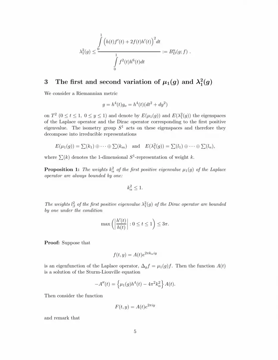
2 The first positive eigenvalue of the Dirac operator andLaplace operator
Let g and go be two conformally equivalent metrics on T 2. Then the Laplace andDirac operators are related by the well-known formulas
∆g =1
h4∆o,
Dg =1
h2Do +
grad (h)
h3,
where grad (h) denotes the gradient of the function h with respect to the metric go.Let us fix the trivial spin structure on T 2. In this case the kernel of the operator Do
coincides with the space of all parallel spinor fields, in particular, any solution of theequation Do(ψo) = 0 has constant length. The kernel of the operator Dg is given by
ker(Dg) =
{
1
hψo : Do(ψo) = 0
}
.
The square D2g of the Dirac operator preserves the decomposition S = S+ ⊕ S− of
the spinor bundle S. Moreover, D2g acts on the space of all sections of S± with the
same eigenvalues. Therefore, the first positive eigenvalue λ21(g) of the operator D2
g
can be computed using sections in the bundle S+ only. Any section ψ ∈ Γ(S+) isgiven by a function f and a parallel spinor field ψo ∈ Γ(S+):
ψ = (f · h)ψo.
The spinor field ψ is L2-orthogonal to the kernel of the operator D2g if and only if
∫
T 2
(ψ, 1hψo)dT
2g = |ψo|2
∫
T 2
fh4dT 2o = 0
holds, where dT 2o and dT 2
g = h4dT 2o are the volume forms of the metrics go and g.
The Rayleigh quotient for the operator D2g is given by
∫
T 2
|Dg(ψ)|2dT 2g
∫
T 2
|ψ|2dT 2g
=
∫
T 2
|h · grad (f) + 2fgrad (h)|2dT 2o
∫
T 2
f2h6dT 2o
.
Finally, we obtain the following formulas for the first positive eigenvalue µ1(g), λ21(g)
of the Laplace operator ∆g and the square D2g of the Dirac operator with respect to
the trivial spin structure:
µ1(g) = inf
∫
T 2
|grad (f)|2dT 2o
∫
T 2
f2h4dT 2o
:
∫
T 2
fh4dT 2o = 0
3

λ21(g) = inf
∫
T 2
|h · grad (f) + 2f · grad (h)|2dT 2o
∫
T 2
f2h6dT 2o
:
∫
T 2
fh4dT 2o = 0
.
A direct calculation yields the formula∫
T 2
|h·grad (f)+2fgrad (h)|2dT 2o =
∫
T 2
h2f∆o(f)dT 2o +
∫
T 2
(4|grad (h)|2+12∆o(h
2))f2dT 2o .
Let us use this formula in case that f is an eigenfunction of the Laplace operator,i.e.,
∆o(f) = µ1(g)h4f.
Then it implies the following inequality between the first eigenvalues of the Laplaceand Dirac operator:
λ21(g) ≤ µ1(g) +
∫
T 2
(
4|grad (h)|2 + 12∆o(h
2))
f2dT 2o
∫
T 2
f2h6dT 2o
.
We are now looking for L2-estimates in case the metric g admits an S1-symmetry.Indeed, let us suppose that the metric g is defined on [0, 1] × [0, 1] by
g = h4(t)go = h4(t)(dt2 + dy2),
where the conformal factor h4 depends on the variable t only. Moreover, we assumethat the function h (t) has the symmetry
h(t) = h(1 − t).
Then any function f(t) with f(t) = −f(1 − t) satisfies the condition
∫
T 2
fh4dT 2o = 0
and, consequently, yields upper bounds for µ1(g) and λ1(g):
µ1(g) ≤
1∫
0
|f ′(t)|2dt
1∫
0
f2(t)h4(t)dt
:= BuL(g; f)
4
λ21(g) ≤
1∫
0
(
h(t)f ′(t) + 2f(t)h′(t))2dt
1∫
0
f2(t)h6(t)dt
:= BuD(g; f) .
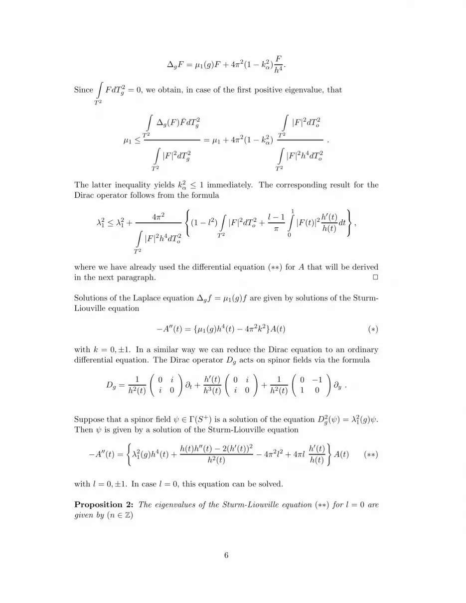
3 The first and second variation of µ1(g) and λ21(g)
We consider a Riemannian metric
g = h4(t)go = h4(t)(dt2 + dy2)
on T 2 (0 ≤ t ≤ 1, 0 ≤ y ≤ 1) and denote by E(µ1(g)) and E(λ21(g)) the eigenspaces
of the Laplace operator and the Dirac operator corresponding to the first positiveeigenvalue. The isometry group S1 acts on these eigenspaces and therefore theydecompose into irreducible representations
E(µ1(g)) =∑
(k1) ⊕ · · · ⊕∑(km) and E(λ21(g)) =
∑
(l1) ⊕ · · · ⊕∑(ln),
where∑
(k) denotes the 1-dimensional S1-representation of weight k.
Proposition 1: The weights k2α of the first positive eigenvalue µ1(g) of the Laplace
operator are always bounded by one:
k2α ≤ 1.
The weights l2β of the first positive eigenvalue λ21(g) of the Dirac operator are bounded
by one under the condition
max
(∣
∣
∣
∣
h′(t)
h(t)
∣
∣
∣
∣
: 0 ≤ t ≤ 1
)
≤ 3π.
Proof: Suppose that
f(t, y) = A(t)e2πkαiy
is an eigenfunction of the Laplace operator, ∆gf = µ1(g)f . Then the function A(t)is a solution of the Sturm-Liouville equation
−A′′(t) ={
µ1(g)h4(t) − 4π2k2
α
}
A(t).
Then consider the function
F (t, y) = A(t)e2πiy
and remark that
5
∆gF = µ1(g)F + 4π2(1 − k2α)F
h4.
Since
∫
T 2
FdT 2g = 0, we obtain, in case of the first positive eigenvalue, that
µ1 ≤
∫
T 2
∆g(F )F dT 2g
∫
T 2
|F |2dT 2g
= µ1 + 4π2(1 − k2α)
∫
T 2
|F |2dT 2o
∫
T 2
|F |2h4dT 2o
.
The latter inequality yields k2α ≤ 1 immediately. The corresponding result for the
Dirac operator follows from the formula
λ21 ≤ λ2
1 +4π2
∫
T 2
|F |2h4dT 2o
(1 − l2)
∫
T 2
|F |2dT 2o +
l − 1
π
1∫
0
|F (t)|2h′(t)
h(t)dt
,
where we have already used the differential equation (∗∗) for A that will be derivedin the next paragraph. 2
Solutions of the Laplace equation ∆gf = µ1(g)f are given by solutions of the Sturm-Liouville equation
−A′′(t) = {µ1(g)h4(t) − 4π2k2}A(t) (∗)
with k = 0,±1. In a similar way we can reduce the Dirac equation to an ordinarydifferential equation. The Dirac operator Dg acts on spinor fields via the formula
Dg =1
h2(t)
(
0 i
i 0
)
∂t +h′(t)
h3(t)
(
0 i
i 0
)
+1
h2(t)
(
0 −11 0
)
∂y .
Suppose that a spinor field ψ ∈ Γ(S+) is a solution of the equation D2g(ψ) = λ2
1(g)ψ.Then ψ is given by a solution of the Sturm-Liouville equation
−A′′(t) =
{
λ21(g)h
4(t) +h(t)h′′(t) − 2(h′(t))2
h2(t)− 4π2l2 + 4πl
h′(t)
h(t)
}
A(t) (∗∗)
with l = 0,±1. In case l = 0, this equation can be solved.
Proposition 2: The eigenvalues of the Sturm-Liouville equation (∗∗) for l = 0 aregiven by (n ∈ Z)
6

λ2 =4π2n2
1∫
0
h2(t)dt
2 .
Proof: The Sturm-Liouville operator
H = − 1
h4(t)
d2
dt2− h(t)h′′(t) − 2(h′(t))2
h6(t)
admits a square root, namely
√H(−) =
i
h3(t)
d
dt(h(t)−).
Since we have ddth2(t)A(t)A(t) = 0, any solution of the equation
i
h3(t)
d
dt(h(t)A(t)) = λA(t)
satisfies the condition
|A(t)| =const
h(t).
Consequently, it makes sense to define a function f : R1 → R
1 by the formula
h(t)A(t) = eif(t),
for which we easily obtain the differential equation f ′(t) = λh2(t). But since A(t)is a periodic solution, we have the condition
2πn =
1∫
0
f ′(t)dt = λ
1∫
0
h2(t)dt
for some integer n ∈ Z, thus yielding the result.
Corollary: Let λ2(g) be an eigenvalue of the Dirac operator on the two-dimensionaltorus T 2 with respect to the trivial spin structure and a Riemannian metric
g = h4(t)(dt2 + dy2)
with isometry group S1. Moreover, suppose that the eigenspinor is S1-invariant(l = 0). Then
λ2(g)vol (T 2, g) ≥ 4π2
holds.
7

Proof: Since the volume is given by vol (T 2, g) =
1∫
0
h4(t)dt, the inequality follows
directly from the Cauchy-Schwarz inequality
1∫
0
h2(t)dt
2
≤1∫
0
h4(t)dt and the
previous Proposition. 2
Remark: This corollary should be compared with the following fact. Fix a re-presentation Σ(k) and denote by µ1(g; k) the first eigenvalue of the Laplace operatorsuch that its eigenspace contains the representation Σ(k). In case k 6= 0 the solutionA(t) of equation (∗) is positive (see [8], page 207) and consequently the inequality
1∫
0
(
4πk2 − µ1(g; k)h4(t)
)
dt ≥ 0
is valid. We thus obtain the estimate
4π2k2 ≥ µ1(g; k)vol (T2, g)
and equality holds if and only if the metric is flat. In particular (k = ±1) we have
4π2 ≥ µ1(g)vol (T2, g)
for the first positive eigenvalue of the Laplace operator in case that its eigenspacecontains the representation Σ(±1).
Let us introduce the Hamiltonian operator Hl defined by the Sturm-Liouville equa-tion (∗∗) for λ2 = 0:
Hl = − d2
dt2+ 4πl2 − 4πl
h′(t)
h(t)− h(t)h′′(t) − 2(h′(t))2
h2(t).
Proposition 3: For l 6= 0, the Hamiltonian operators Hl are strictly positive. Ho isa non-negative operator.
Proof: A direct calculation yields the formula
1∫
0
Hl
(
ϕ(t)
h(t)
)
ϕ(t)
h(t)dt =
1∫
0
(
2πlϕ(t)
h(t)− ϕ′(t)
h(t)
)2
dt ≥ 0
where ϕ(t) is any periodic function. The equation 2πlϕ(t)−ϕ′(t) = 0 does not admita periodic, non-trivial solution in case l 6= 0. Consequently, Hl is a strictly positiveoperator for l 6= 0.
Corollary: Fix an S1-representation∑
(l). Let λ21(g, l) be the first eigenvalue of
the Dirac operator on the two-dimensional torus T 2 with respect to the trivial spinstructure and an S1-invariant metric
8

g = h4(t)(dt2 + dy2)
such that the representation∑
(l) occurs in the decomposition of the eigenspace. Thenthe multiplicity of
∑
(l) is one and the eigenspinor does not vanish anywhere (l 6= 0).
Proof: Since Hl is strictly positive, the eigenvalue λ2(g) is the unique positivenumber λ2 such that
inf spec(Hl − λ2h4) = 0.
The corresponding real solution of this Sturm-Liouville equation is unique and posi-tive (see [8], page 207).
Corollary: For a fixed S1-representation∑
(l) denote by λ21(g, l) the first eigenvalue
of the Dirac operator such that the eigenspace E(λ21(g, l)) contains the representation
∑
(l). Then the inequality
λ21(g, l) ≤
1∫
0
(2πlϕ(t) − ϕ′(t))2
h2(t)dt
1∫
0
h2(t)ϕ2(t)dt
holds for any periodic function ϕ(t).
Proof: Since inf spec(Hl − λ21(g, l)h
4) = 0, we have
1∫
0
Hl
(
ϕ
h
)
ϕ
h(t)dt − λ2
1(g, l)
1∫
0
h2(t)ϕ2(t)dt ≥ 0
for any periodic function ϕ(t).
In case of the flat metric go = dt2 + dy2 we have µ1(go) = λ21(go) = 4π2 and
E(µ1(go)) =∑
(0) ⊕∑(0) ⊕∑(1) ⊕∑(−1) = E(λ21(go)).
The spaces∑
(±1) correspond to the case that k = l = ±1 and are generated bythe constant function. The two spaces
∑
(0) are generated by the functions sin(2πt),cos(2πt).
Notation: We introduce now a few notations which will be used throughout thisarticle. Let us consider a deformation gE = h4
E(t)go of the flat metric go dependingon some parameter E. We assume that
h4E(t) = h4
E(1 − t)
9

holds for all parameters of the deformation. The eigenvalues µ1(go) and λ21(go) of
multiplicity four split into three eigenvalues
µ1(go) 7→ {µ1(E), µ2(E), µ3(E)} , λ21(go) 7→ {λ2
1(E), λ22(E), λ2
3(E)}.
The eigenvalue µ3(E) corresponds to the case that k = ±1, has multiplicity two,and its eigenfunction is a deformation of the constant function. The eigenvaluesµ1(E) 6= µ2(E) correspond to solutions of the Sturm-Liouville equation (∗) andtheir eigenfunctions are deformations of sin (2πt) and cos (2πt), respectively. Thesituation is different for the Dirac equation: there, according to Proposition 2, thetrivial S1-representation (l = 0) yields one eigenvalue λ2
1(E) of multiplicity two andthe non-trivial representations (l = ±1) define in general two distinct eigenvaluesλ2
2(E), λ23(E) of multiplicity one. However, in case hE(t) = hE(1 − t), the spectral
functions λ22(E) and λ2
3(E) coincide. Obviously, for small values E ≈ 0 we have
µ1(gE) = min {µ1(E), µ2(E), µ3(E)} , λ21(gE) = min {λ2
1(E), λ32(E), λ2
3(E)}.
We will compute the first and second variation of µα(E) and λ2α(E) at E = 0. For
this purpose we introduce the following notation: Let A be a function depending bothon E and t. Then A denotes the derivative with respect to E and A′ the derivativewith respect to t. Moreover, we expand the function h4
E(t) in the form
h4E(t) = 1 + EH(t) + E2G(t) + O(E3).
Theorem 1: Consider a deformation
gE = (1 + EH(t) + E2G(t) + O(E3))go = h4E(t)go
of the flat metric on the torus T 2 such that h4E(t) = h4
E(1 − t). Moreover, supposethat for E 6= 0 and k = 0 the eigenvalues µ1(E) 6= µ2(E) are simple eigenvalues ofthe Sturm-Liouville equation (∗). Then
a.) µ1(0) = −8π2
1∫
0
H(t) sin2 (2πt)dt , µ2(0) = −8π2
1∫
0
H(t) cos2 (2πt)dt
µ3(0) = −4π2
1∫
0
H(t)dt.
b.) λ21(0) = λ2
2(0) = λ23(0) = −4π2
1∫
0
H(t)dt.
In particular, we obtain
µ1(0) + µ2(0) = 2µ3(0) = 2λ2α(0).
10

Corollary: Suppose that the deformation
gE = (1 + EH(t) + E2G(t) + O(E3))go
of the flat metric go satisfies the condition
H(t) = H(1 − t)
as well as
1∫
0
H(t) sin2 (2πt)dt 6=1∫
0
H(t) cos2(2πt)dt.
Then, for all parameters E 6= 0 near zero we have the strict inequality
µ1(gE) < λ21(gE).
Next we compute the second variation of our spectral functions under the assumptionthat the first variation is trivial.
Theorem 2: Consider a deformation
gE = (1 + EH(t) + E2G(t) + O(E3))go = h4E(t)go
of the flat metric go on the torus T 2 and suppose that the conditions
h4E(t) = h4
E(1 − t)
and
1∫
0
H(t) sin2 (2πt)dt =
1∫
0
H(t) cos2 (2πt)dt = 0
are satisfied. Moreover, suppose that for E 6= 0 and k = 0 the eigenvalues µ1(E) 6=µ2(E) are simple eigenvalues of the Sturm-Liouville equation (∗). Then
a.) µ1(0) = −16π2
1∫
0
G(t) sin2 (2πt)dt − 16π2
1∫
0
H(t)C(t) sin (2πt)dt,
where C(t) is the periodic solution of the differential equation
C ′′(t) = −4π2H(t) sin (2πt) − 4π2C(t).
b.) µ2(0) = −16π2
1∫
0
G(t) cos2(2πt) − 16π2
1∫
0
H(t)C(t) cos(2πt)dt,
where C(t) is the periodic solution of the differential equation
C ′′(t) = −4π2H(t) cos(2πt) − 4π2C(t).
11

c.) µ3(0) = −8π2
1∫
0
G(t)dt − 8π2
1∫
0
H(t)C(t)dt,
where C(t) is the periodic solution of the differential equation
C ′′(t) = −4π2H(t).
d.) λ21(0) = −8π2
1∫
0
G(t)dt + 2π2
1∫
0
H2(t)dt
e.) λ22(0) = λ2
3(0) = −8π2
1∫
0
G(t)dt + 4π2
1∫
0
H2(t)dt − 8π2
1∫
0
H(t)C(t)dt
−2π
1∫
0
H ′(t)C(t)dt,
where C(t) is the periodic solution of the differential equation
C ′′(t) = −4π2H(t) − πH ′(t).
Proof of Theorem 1 and Theorem 2: The formulas for the derivatives of λ21(E)
are a direct consequence of Proposition 2. We will prove the variation formulas forλ2
3 and just remark that one can investigate the other spectral functions in a similarway. Moreover, since all the calculations we make are up to order two with respectto E, we may assume for simplicity that
h4E(t) = 1 + EH(t) + E2G(t).
We compute
hEh′′
E − 2(h′E)2
h2E
=1
4E
H ′′ + EG′′
(1 + EH + E2G)− 5
16E2 (H ′ + EG′)2
(1 + EH + E2G)2
and, consequently, we obtain the formulas
d
dE
(
hEh′′
E − 2(h′E)2
h2E
)
E=0
=1
4H ′′ ,
d
dE
(
h′EhE
)
E=0=
1
4H ′
d2
dE2
(
hEh′′
E − 2(h′E)2
h2E
)
E=0
=1
2(G′′ −H ′′H) − 5
8(H ′)2.
The spectral function λ23(E) is defined by a periodic solution AE(t) of the Sturm-
Liouville equation
A′′
E(t) = −λ23(E)h4
E(t)AE(t)−hE(t)h′′E(t) − 2(h′E(t))2
h2E(t)
AE(t)+4π2AE(t)−4πh′E(t)
hE(t)AE(t)
12
with the initial conditions λ23(0) = 4π2, Ao(t) ≡ 1. Therefore, we obtain
A′′
o(t) = −λ23(0) − 4π2H(t) − 4π2Ao(t) −
1
4H ′′(t) + 4π2Ao(t) − πH ′(t)
in this case and, consequently,
λ23(0) = −4π2
1∫
0
H(t)dt.
Let us now compute the second variation in case that λ21(0) = 0 = λ2
3(0). Wedifferentiate the Sturm-Liouville equation twice at E = 0:
A′′
o(t) = −λ23(0) − 8π2G(t) − 8π2H(t)Ao(t) +
5
8(H ′(t))2 − 1
2
(
G′′(t) −H ′′(t)H(t))
−1
2H ′′(t)Ao(t) − 2πH ′(t)Ao(t) − 4π
d
dt
(
d2
dE2(ln (hE(t)))E=0
)
.
Then we obtain
λ23(0) = −8π2
1∫
0
G(t)dt − 8π2
1∫
0
H(t)Ao(t)dt +
(
5
8− 1
2
)
1∫
0
(H ′(t))2dt
−1
2
1∫
0
H ′′(t)Ao(t)dt − 2π
1∫
0
H ′(t)Ao(t)dt.
Since Ao(t) is a solution of the differential equation
A′′
o(t) = −4π2H(t) − 1
4H ′′(t) − πH ′(t),
we have
−1
2
1∫
0
H ′′(t)Ao(t)dt = −1
2
1∫
0
H(t)A′′
o(t)dt = +1
2
1∫
0
H(t)
(
4π2H(t) +1
4H ′′(t)
)
dt
= 2π2
1∫
0
H2(t)dt − 1
8
1∫
0
(H ′(t))2dt
and, consequently, we obtain
λ23(0) = −8π2
1∫
0
G(t)dt + 2π2
1∫
0
H2(t)dt − 8π2
1∫
0
H(t)Ao(t)dt − 2π
1∫
0
H ′(t)Ao(t)dt
= −8π2
1∫
0
G(t)dt + 4π2
1∫
0
H2(t)dt − 8π2
1∫
0
H(t)C(t)dt− 2π
1∫
0
H ′(t)C(t)dt,
13

where C(t) := Ao(t) + 14H(t) is a solution of the differential equation
C ′′(t) = −4π2H(t) − πH ′(t).
Corollary: λ23(0) = µ3(0) + 2π2
1∫
0
H2(t)dt.
In particular, for all parameters E 6= 0 near zero we have the inequality
µ3(E) < λ23(E).
Moreover, the first positive eigenvalue µ1(gE) of the Laplace operator is alwayssmaller then the corresponding eigenvalue λ2
1(gE) of the Dirac operator for any metricgE near E ≈ 0, i.e.,
µ1(gE) < λ21(gE).
Remark: The explicit formulas in Theorem 1 and Theorem 2 can be generalizedto the case of an arbitrary conformal deformation. Fix a Riemannian metric go on asurface M2 and consider the deformation
gE = (1 + EH + E2G+ O(E3))go
of the metric. Moreover, suppose that µ1(E) is the deformation of the eigenvalue ofthe Laplace operator and fE is the corresponding family of eigenfunctions. Then thefollowing formulas hold:
a.) µ1(0) = −µ1(0)
∫
M2
Hf2odM
2o
∫
M2
f2o dM
2o
b.) µ1(0) = −2µ1(0)
∫
M2
(Gf2o + Cfo)dM
2o
∫
M2
f2o dM
2o
,
where the function C is the solution of the differential equation
∆oC = µ1(0)Hfo + µ1(0)C.
The corresponding expression for the variation of the eigenvalue λ1(E) of the Diracoperator can also be computed:
14

c.) λ1(0) = −λ1(0)
∫
M2
H · |ψo|2dM2o
2
∫
M2
|ψo|2dM2o
and a similar formula holds for the second variation.
Once again, a similar, though even more intricate computation yields the fourth vari-ation of λ2
3(E) under the assumption that all previous variations of λ23(E) vanish.
This is needed for the discussion of the example in Section 5.
Theorem 3: Consider a deformation
gE = (1 + EH(t))go
of the flat metric go on the torus T 2 and suppose that the following conditions aresatisfied:
a.) H(t) = H(1 − t);
b.) λ23(0) = λ2
3(0) =···
λ23 (0) = 0 .
Then the fourth derivative [λ23(0)]
(IV) of the spectral function λ23(E) at E = 0 is given
by the formula
[λ23(0)]
(IV) = 6
1∫
0
H3(t)H ′′(t)dt +45
2
1∫
0
H2(t)(H ′(t))2dt−1∫
0
(
16π2H(t) +H ′′(t))
C3(t)dt
+
1∫
0
(
5
2(H ′(t))2 + 2H(t)H ′′(t)
)
C2(t)dt
−1∫
0
(
15(H ′(t))2 + 6H ′′(t)H(t))
H(t)C1(t)dt,
where the functions C1(t), C2(t), C3(t) are periodic solutions of the equations
C ′′
1 (t) = −4π2H(t) − 1
4H ′′(t) − πH ′(t)
C ′′
2 (t) =1
2H(t)H ′′(t) +
5
8(H ′(t))2 + 2πH ′(t)H(t) −
(
8π2H(t) +1
2H ′′(t) + 2πH ′(t)
)
C1(t)
C ′′
3 (t) = −(
3
2H ′′(t)H2(t) +
15
4H(t)(H ′(t))2 + 6πH ′(t)H2(t)
)
+
(
3
2H(t)H ′′(t) +
5
8(H ′(t))2 + 6H(t)H ′(t)
)
C1(t)
−(
3πH ′(t) +3
4H ′′(t) + 4π2H(t)
)
C2(t).
15

Remark: In the special case of H ′′(t) = −16π2H(t) the derivative [λ23(0)]
(IV) doesnot depend on C3(t) and the formulas become much simpler. Such a metric will bethe object of Section 5.
4 Examples
4.1 The variation gE = (1 + E cos(2πt))go
The volume vol (T 2, gE) = 1 of this variation of the flat metric go is constant and allfirst derivatives at E = 0 vanish since
1∫
0
cos(2πt) cos2(2πt) =
1∫
0
cos(2πt) sin2(2πt) = 0.
A computation of the second derivatives yields the following numerical values:
µ1(0) = −2
3π2 , µ2(0) =
10
3π2 , µ3 = −4π2
λ21(0) = π2 , λ2
2(0) = λ23(0) = −3π2.
In particular, we obtain
µ1(gE) < λ21(gE)
for all parameters E 6= 0 near zero. The eigenspinor corresponding to the minimalpositive eigenvalue of the Dirac operator does not vanish anywhere (Figure 1).
λ2(Ε)
λ2(Ε)=λ2(Ε)µ1(Ε) µ3(Ε)
µ2(Ε)
2
-0.1 -0.05 0.05 0.1
39.45
39.46
39.47
39.48
39.49
1
3
(Figure 1)
16

4.2 The Mathieu deformation gE = (1 + E cos(4πt))go of the flatmetric
This deformation of the flat metric again preserves the volume, and the Laplaceequation essentially reduces to the classical Mathieu equation u′′(x) + (a +16q cos(2x))u(x) = 0. In this case the first variation is trivial only for the Diracequation. Indeed, we have
µ1(0) = 2π2 , µ2(0) = −2π2 , µ3(0) = 0
λ21(0) = λ2
2(0) = λ23(0) = 0.
Even for the Mathieu deformation we conclude that
µ1(gE) < λ21(gE)
for E 6= 0 near zero. A computation of the second derivatives yields the followingresult (Figure 2):
µ3(0) = −π2 , λ21(0) = π2 , λ2
2(0) = λ23(0) = 0.
For a detailed discussion of this metric, we refer to the next section.
µ3(Ε)
µ2(Ε) µ1(Ε)
λ (Ε)1
-0.3 -0.2 -0.1 0.1 0.2 0.3
38.75
39.25
39.5
39.75
40
40.25
2
λ (Ε)= λ (Ε)2 22 3
(Figure 2)
17
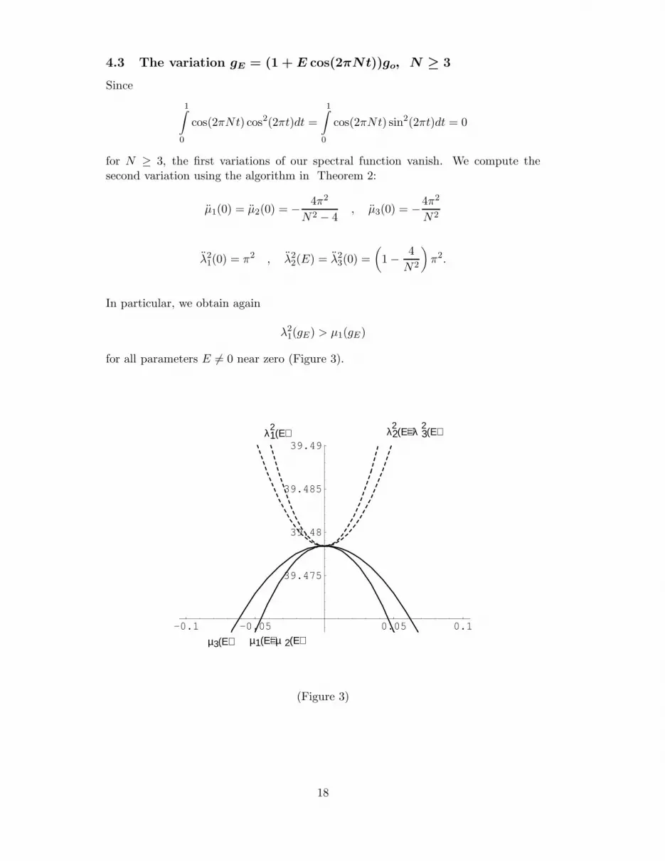
4.3 The variation gE = (1 + E cos(2πNt))go, N ≥ 3
Since
1∫
0
cos(2πNt) cos2(2πt)dt =
1∫
0
cos(2πNt) sin2(2πt)dt = 0
for N ≥ 3, the first variations of our spectral function vanish. We compute thesecond variation using the algorithm in Theorem 2:
µ1(0) = µ2(0) = − 4π2
N2 − 4, µ3(0) = −4π2
N2
λ21(0) = π2 , λ2
2(E) = λ23(0) =
(
1 − 4
N2
)
π2.
In particular, we obtain again
λ21(gE) > µ1(gE)
for all parameters E 6= 0 near zero (Figure 3).
λ1(Ε)
µ3(Ε) µ1(Ε)=µ2(Ε)
λ2(Ε)=λ3(Ε)2 2 2
-0.1 -0.05 0.05 0.1
39.475
39.48
39.485
39.49
(Figure 3)
18

5 The Mathieu deformation of the flat metric
In the previous examples, the deformation
gE = (1 + E cos(4πt))go
of the flat metric go plays an exceptional role, because the derivatives µ1(0), µ2(0) 6= 0are non-zero. Therefore, we study the behaviour of the first positive eigenvalue forthe Laplace and Dirac operator in more detail. First of all, the lower bound
4π2
h4max
≤ µ1(E), λ21(E)
yields the estimate
4π2
1 + |E| ≤ µ1(E), λ21(E)
for all parameters −1 < E < 1. In case of the function f(t) = sin(2πt) the upperbound Bu
L(g, f) of Section 2 leads to the estimate
µ1(E) ≤ 8π2
2 + |E| ,
i.e., for all parameters −1 < E < 1 the inequality
4π2
1 + |E| ≤ µ1(E) ≤ 8π2
2 + |E|
holds. On the other hand, for the Dirac operator the function
f(t) = (1 + E cos(4πt))14 sin(2πt)
gives an upper bound BuD(gE , f) for its first eigenvalue with the property
limE→−1
BuD(gE , f) = 5π2.
We will thus investigate the limits limE→−1
µ1(E) as well as limE→−1
λ21(E). The eigenvalue
µ1(E) is related with a periodic solution of the Sturm-Liouville equation
A′′(t) = −µ1(E)(
1 + E cos(4πt))
A(t) + 4π2k2A(t),
where k = 0,±1 (see Proposition 1). Let us introduce the function B(x) := A(
12πx)
where 0 ≤ x ≤ 2π. Then the Sturm-Liouville equation is equivalent to the classicalMathieu equation
B′′(x) + (a+ 16q cos(2x))B(x) = 0,
where the parameters a and q are given by
19

a =µ1(E)
4π2− k2 , q =
Eµ1(e)
16(4π2), k = 0,±1.
For E → −1 the parameters of the Mathieu equation are related by
a = −16q − k2 , k = 0,±1.
Using the estimates for µ1(E) we obtain
2π2 ≤ limE→−1
µ1(E) ≤ 8
3π2,
i.e., − 1
24≤ q ≤ − 1
32in case E = −1.
A numerical computation shows that, under these restrictions, the Mathieu equationhas a unique periodic solution for k = 0 and q ≈ 0, 04113. This solution B(x) isthe first Mathieu function se1(x, q), which is the deformation of the function sin(x).Consequently, we have
limE→−1
µ1(E) = −16 · q · 4π2 ≈ 2, 6323π2.
The limits of the spectral functions µ2(E) and µ3(E) can be computed in a similarway:
limE→−1
µ2(E) ≈ 1, 79 · (4π2) , limE→−1
µ3(E) ≈ 0, 9 · (4π2).
These limits correspond to the Mathieu functions ce1(x, q) and ceo(x, q) for the pa-rameters q ≈ −0, 112 in case of µ2(E) and q ≈ −0, 056296 in case of µ3(E).
-1 -0.8 -0.6 -0.4 -0.2
25
30
35
µ3(Ε)
µ1(Ε) lower bound
BLu
4π2
2π2
(2,63)π2(2,66)π2
(3,6)π2
(Figure 4)
20

Approximation of the periodic solution for µ1(E), E → −1 :
NDSolve[{y’’[x] + 32(0.04113)(Sin[x])^2 y[x] == 0,
y[x] == 0 , y’[0] == 1} , y , {x , 0 , 10 Pi}]
Plot[Evaluate[y[x]/.% , {x , 0 , 10 Pi}]
5 10 15 20 25 30
-1
-0.5
0.5
1
(Figure 5)
Approximation of the periodic solution for µ2(E), E → −1 :
NDSolve[{y’’[x] + 32(0.1112)(Sin[x])^2 y[x] == 0,
y[x] == 1 , y’[0] == 0} , y , {x , 0 , 10 Pi}]
Plot[Evaluate[y[x]/.% , {x , 0 , 10 Pi}]
5 10 15 20 25 30
-1
-0.5
0.5
1
(Figure 6)
21
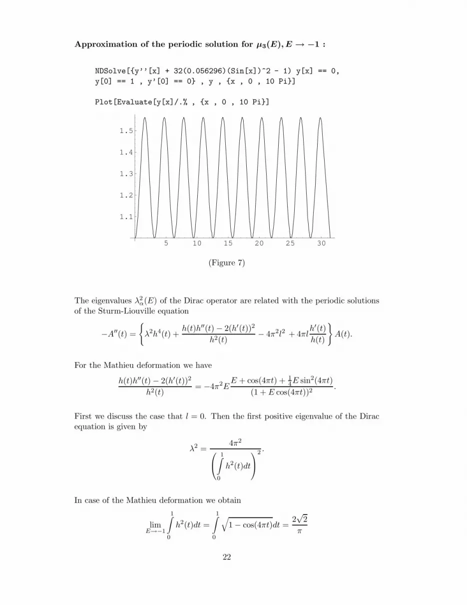
Approximation of the periodic solution for µ3(E), E → −1 :
NDSolve[{y’’[x] + 32(0.056296)(Sin[x])^2 - 1) y[x] == 0,
y[0] == 1 , y’[0] == 0} , y , {x , 0 , 10 Pi}]
Plot[Evaluate[y[x]/.% , {x , 0 , 10 Pi}]
5 10 15 20 25 30
1.1
1.2
1.3
1.4
1.5
(Figure 7)
The eigenvalues λ2α(E) of the Dirac operator are related with the periodic solutions
of the Sturm-Liouville equation
−A′′(t) =
{
λ2h4(t) +h(t)h′′(t) − 2(h′(t))2
h2(t)− 4π2l2 + 4πl
h′(t)
h(t)
}
A(t).
For the Mathieu deformation we have
h(t)h′′(t) − 2(h′(t))2
h2(t)= −4π2E
E + cos(4πt) + 14E sin2(4πt)
(1 + E cos(4πt))2.
First we discuss the case that l = 0. Then the first positive eigenvalue of the Diracequation is given by
λ2 =4π2
1∫
0
h2(t)dt
2 .
In case of the Mathieu deformation we obtain
limE→−1
1∫
0
h2(t)dt =
1∫
0
√
1 − cos(4πt)dt =2√
2
π
22

and, finally,
limE→−1
λ2(E) =1
2π4 ≈ (4, 92)π2
-1 -0.8 -0.6 -0.4 -0.2
25
30
35
40
45
50
lower bound
BuD
4 π²
2 π²
5 π²(4,92) π²
λ2 (E)1
(Figure 8)
We now investigate the case l = 1. Let us consider the Hamiltonian operator HE
given by the Sturm-Liouville equation for λ2 = 0:
HE = − d2
dt2+ 4π2 − 4π
h′(t)
h(t)− h(t)h′′(t) − 2(h′(t))2
h2(t)= − d2
dt2+ pE(t),
where the potential pE(t) is given by the formula
pE(t) = 4π2 + Eπ2 4 cos(4πt) + 4 sin(4πt) + E sin2(4πt) + 2E(2 + sin(8πt))
(1 + E cos(4πt))2.
For all parameters −1 < E ≤ 0 the Hamiltonian operator HE is strictly positive (seeProposition 3). Consequently, the eigenvalue λ2
3(E) is the first number such that
inf spec (HE − λ2(1 + E cos(4πt))) = 0,
and the corresponding solution of the Sturm-Liouville equation
A′′
E(t) = (pE(t) − λ23(E)(1 +E cos(4πt)))AE(t)
is unique and everywhere positive. In particular, the solution satisfies the condition
AE(t+ 12) = AE(t).
23

Since AE(t) is a positive periodic solution of the Sturm-Liouville equation, we obtainthe condition
1∫
0
(pE(t) − λ23(E)(1 + E cos(4πt)))dt > 0
and thus an upper bound for λ23(E):
λ23(E) <
1∫
0
pE(t)dt.
-0.5 -0.4 -0.3 -0.2 -0.1
39.5
39.75
40.25
40.5
40.75
41
upper bound for λ (Ε)23
(Figure 9)
We notice that this upper bound for λ23(E) grows and reflects, indeed, the real
behaviour of λ23(E) near E = 0. To see this, we use Theorem 3 to compute the
fourth variation of this spectral function (the third variation vanishes since λ23(E)
has to be a symmetric function in E). One obtains the following result:
[λ23(0)]
(IV) =27
4π2 > 0.
On the other hand, using well-known approximation techniques for Sturm-Liouvilleequations with periodic coefficients (see [9]) we can approximate λ2
3(E) for a fixedparameter E. Indeed, one replaces the potential in the Sturm-Liouville equation bythe first terms of its Fourier series. This reduces the computation of the approxima-tive eigenvalue to a finite-dimensional eigenvalue problem. For example, in case ofE = −0.3 the mentioned methods yields the result
λ23(−0.3) ≈ 39.6733.
Let us study the behaviour of the spectral function λ23(E) for E → −1. More
generally, denote by λ2(E, l) the first eigenvalue of the Dirac operator such that the
24
corresponding eigenspace contains an S1-representation of weight l. In particular,we have λ2
3(E) = λ2(E, 1) = λ2(E,−1). We apply the Corollary of Proposition 3 tothe function hE(t) = 4
√
1 + E cos(4πt) and conclude that
1∫
0
(2πlϕ(t) − ϕ′(t))2√
1 + E cos(4πt)− λ2(E, l)
1∫
0
√
1 + E cos(4πt)ϕ2(t)dt ≥ 0
holds for any periodic function ϕ(t). Fix a test function ϕ(t) and consider the limitE → −1. Then we obtain the inequality
limE→−1
λ2(E, l) ≤ 1
2
1∫
0
(2πlϕ(t) − ϕ′(t))2
| sin(2πt)| dt
1∫
0
| sin(2πt)|ϕ2(t)dt
.
We apply this estimate to the function
ϕl(t) =cos(2πt) + l sin(2πt)
2(l2 + 1)π.
Then 2πlϕl(t) − ϕ′
l(t) = sin(2πt) and we obtain the following
Proposition 4:
limE→−1
λ2(E, l) ≤ 6π2 (l2 + 1)2
(1 + 2l2).
Remark: At E = 0 we have λ2(0, l) = 4π2l2. On the other hand, for l ≥ 3 theinequality
6 · (l2 + 1)2
1 + 2l2< 4l2
holds, i.e.,
limE→−1
λ2(E, l) < λ2(0, l) l ≥ 3.
The latter inequality means that the eigenvalue λ2(E, l) decreases for E → −1(l ≥ 3).
The behaviour of λ23(E) = λ2(E, l) for l = 1 is completely different. This spectral
function increases for E → −1. Using the formula
λ23(E) = inf
ϕ>0
1∫
0
(2πlϕ(t) − ϕ′(t))2√
1 + E cos(4πt)
1∫
0
√
1 + E cos(4πt)ϕ2
25

we can approximate the positive minimizing Mathieu spinor MS (E, t) of topologicalindex l = 1 by expanding it in its Fourier series. We thus obtain for example:
E = −0.9: λ23(−0.9) ≈ 40.1464
MS(-0.9,t)=(Sqrt[Sqrt[1+ (-0.9)Cos[4 Pi t]]]) Sqrt[1+ (0.44)Sin[4 Pi t]
+ (0.15)Cos[4 Pi t] + (0.09)Sin[8 Pi t] + (0.17)Cos[8 Pi t]
+ (0.028)Sin[16 Pi t] + (0.051)Cos[16 Pi t] + (0.051)Sin[12 Pi t]
+ (0.085)Cos[12 Pi t] + (0.016)Sin[20 Pi t] + (0.026)Cos[20 Pi t]
+ (0.01)Sin[24 Pi t] + (0.014)Cos[24 Pi t] + (0.005)Sin[28 Pi t]
+ (0.007)Cos[28 Pi t] + (0.0033)Sin[32 Pi t] + (0.0044)Cos[32 Pi t]]
E = −0.95: λ23(−0.9) ≈ 44.6024
MS(-0.95,t)=(Sqrt[Sqrt[1+ (-0.95)Cos[4 Pi t]]])Sqrt[1+ (0.585)Sin[4 Pi t]
+ (0.049)Cos[4 Pi t] + ( 0.1)Sin[8 Pi t] + (0.08)Cos[8 Pi t]
+ (0.063)Sin[12 Pi t] + (0.063)Cos[12 Pi t] + (0.041)Sin[16 Pi t]
+ (0.04)Cos[16 Pi t] + (0.026)Sin[20 Pi t] + (0.026)Cos[20 Pi t]
+ (0.017)Sin[24 Pi t] + (0.018)Cos[24 Pi t] + (0.012)Sin[28 Pi t]
+ (0.011)Cos[28 Pi t] + (0.008)Sin[32 Pi t] + (0.007)Cos[32 Pi t]]
Finally, we can compute the limit limE→−1
λ23(E) replacing again the potential in the
Sturm-Liouville equation by the first terms of its Fourier series. For E = −1 thisamounts to studying the differential equation
sin2(2πt)A′′(t) =
{
1
2π2(
9 − 3 cos(4πt) − 4 sin(4πt))
− 2λ23 sin4(2πt)
}
A(t)
and the finite-dimensional approximation yields the result
limE→−1
λ23(E) ≈ 47.2437.
Remark: The second variation formulas prove that, in case of the familygE = (1+E cos(2πt))go (N = 1), the minimal positive eigenvalues of the Laplace andDirac operator decrease (see Example 4.1) and are smaller than 4π2. The numericalevaluation of µ3(E) and λ2
3(E) yields the following table:
E 0 -0.1 -0.3 -0.5 -0.7 -0.9 -0.95 -0.99 -1
µ3 4π2 39.284 37.897 35.741 33.378 31.09 30.5 30.1 30.013
λ23 4π2 39.333 38.353 36.714 34.983 33.331 33.2830 36.04 ≈ 36.2
26

6 Final remarks
As shown previously, any local deformation gE of the flat metric realizes the inequal-ity
µ1(gE) < λ21(gE)
between the first eigenvalues of the Laplace and Dirac operator up to second order.We are not able to give an example of a Riemannian metric g on T 2 such thatλ2
1(g) < µ1(g) holds. Moreover, denote again by λ21(g; l) the first positive eigenvalue
of the Dirac operator such that the eigenspace contains an S1-representation of weightl ∈ Z. The corresponding eigenvalue of the Laplace operator we shall denote byµ1(g; l). It is a matter of fact that in all families of Riemannian metrics we havediscussed these two eigenvalues are very close. Let us consider, for example, themetric gE by the function
hE(t) = eE
π(sin(2πt)−2 cos(2πt)).
For the parameter E = 1 we obtain the following numerical values using theapproximation method described before in the space spanned by the functions1, sin(2πnt), cos(2πnt) (1 ≤ n ≤ 5):
λ21(g; 1) ≈ 6.11056 , µ1(g; 1) ≈ 5.19025.
However, even in this case we already have the inequality µ1(gE ; 1) < λ21(gE ; 1) and
the following figure shows the graph of the two spectral functions for 0 ≤ E ≤ 1 (forthe first and the second positive eigenvalue):
10
20
30
40
50
60
70
80
90
x
0 0.2 0.4 0.6 0.8 1E
(Figure 10)
27

References
[1] I. Agricola, Th. Friedrich. Upper bounds for the first eigenvalue of the Diracoperator on surfaces, to appear in ”Journal of Geometry and Physics”.
[2] B. Ammann. Spin-Strukturen und das Spektrum des Dirac-Operators, Disser-tation Freiburg 1998, Shaker-Verlag Aachen 1998.
[3] Chr. Bar. Lower eigenvalues estimates for Dirac operators, Math. Ann. 293(1992), 39-46.
[4] Th. Friedrich. Dirac-Operatoren in der Riemannschen Geometrie, Vieweg-VerlagBraunschweig/ Wiesbaden 1997.
[5] P. Hartman. Ordinary differential equations, New York 1964.
[6] P. Li, S.T. Yau. A new conformal invariant and its application to the Willmoreconjecture and the first eigenvalue of compact surfaces, Invent. Math. 69 (1982),269-291.
[7] J. Lott. Eigenvalue bounds for the Dirac operator, Pac. Journ. Math. 125 (1986),117-128.
[8] M. Reed, B. Simon. Methods of modern mathematical physics, Part IV, Aca-demic Press Boston 1978.
[9] E.T. Whittaker, G.N. Watson. A course of modern analysis, Cambridge Univer-sity Press 1927.
ILKA AGRICOLAHumboldt-Universitat zu Berlin, Institut fur Mathematik, Sitz: Ziegelstraße 13a,Unter den Linden 6, D-10099 Berline-mail: [email protected]
BERND AMMANNUniversitat Freiburg, Mathematisches Institut, Eckerstr. 1, D-79104 Freiburge-mail: [email protected]
THOMAS FRIEDRICHHumboldt-Universitat zu Berlin, Institut fur Mathematik, Sitz: Ziegelstraße 13a,Unter den Linden 6, D-10099 Berline-mail: [email protected]
28