Embed Size (px)
Citation preview

University of Tennessee, Knoxville University of Tennessee, Knoxville
TRACE: Tennessee Research and Creative TRACE: Tennessee Research and Creative
Exchange Exchange
Masters Theses Graduate School
5-2007
A Crosslayer Routing Protocol (XLRP) for Wireless Sensor A Crosslayer Routing Protocol (XLRP) for Wireless Sensor
Networks Networks
Raghul Gunasekaran University of Tennessee - Knoxville
Follow this and additional works at: https://trace.tennessee.edu/utk_gradthes
Part of the Electrical and Computer Engineering Commons
Recommended Citation Recommended Citation Gunasekaran, Raghul, "A Crosslayer Routing Protocol (XLRP) for Wireless Sensor Networks. " Master's Thesis, University of Tennessee, 2007. https://trace.tennessee.edu/utk_gradthes/285
This Thesis is brought to you for free and open access by the Graduate School at TRACE: Tennessee Research and Creative Exchange. It has been accepted for inclusion in Masters Theses by an authorized administrator of TRACE: Tennessee Research and Creative Exchange. For more information, please contact [email protected].

To the Graduate Council:
I am submitting herewith a thesis written by Raghul Gunasekaran entitled "A Crosslayer Routing
Protocol (XLRP) for Wireless Sensor Networks." I have examined the final electronic copy of this
thesis for form and content and recommend that it be accepted in partial fulfillment of the
requirements for the degree of Master of Science, with a major in Electrical Engineering.
Hairong Qi, Major Professor
We have read this thesis and recommend its acceptance:
Dayakar Penumadu, Itamar Elhanany
Accepted for the Council:
Carolyn R. Hodges
Vice Provost and Dean of the Graduate School
(Original signatures are on file with official student records.)

To the Graduate Council:
I am submitting herewith a thesis written by Raghul Gunasekaran entitled “A Cross-
layer Routing Protocol (XLRP) for Wireless Sensor Networks”. I have examined the
final electronic copy of this thesis for form and content and recommend that it be
accepted in partial fulfillment of the requirements for the degree of Master of Science,
with a major in Electrical Engineering.
Hairong Qi, Major Professor
We have read this thesisand recommend its acceptance:
Dayakar Penumadu
Itamar Elhanany
Accepted for the Council:
Carolyn Hodges
Vice Provost and Dean ofGraduate School

A Crosslayer Routing Protocol for
Wireless Sensor Networks
A Thesis
Presented for the
Master of Science Degree
The University of Tennessee, Knoxville
Raghul Gunasekaran
May 2007

Copyright c© 2007 by Raghul Gunasekaran.
All rights reserved.
ii

Acknowledgments
First and foremost, I would like to thank my advisor Dr.Hairong Qi for the motivation
and guidance, without which this work would not have been possible. I also thank her
for the opportunity to be a part of Advanced Imaging and Collaborative Information
Processing lab. I would like to thank Dr.Dayakar Penumadu and Dr.Itamar Elhanany
for serving on my committee. I would also like to thank Teja Kuruganti for his
valuable support and suggestions on my masters thesis. Not to forget my fellow
AICIP members, who had been of great help and for the great good times we had at
work. Finally, I would also like to thank my family and friends for the support and
encouragement in every possible way, without their support things would have been
very difficult.
iii

Abstract
The advent of wireless sensor networks with emphasis on the information being routed,
rather than routing information has redefined networking from that of conventional
wireless networked systems. Demanding the need for content based routing techniques
and development of low cost network modules, built to operate in large numbers in
a networked fashion with limited resources and capabilities. The unique characteris-
tics of wireless sensor network’s have questioned the applicability and effectiveness of
conventional algorithms defined for wireless ad-hoc networks, leading to the design
and development of protocols specific to wireless sensor network. Many network layer
protocols have been proposed for wireless sensor networks, identifying and address-
ing factors influencing network layer design, this thesis defines a cross layer routing
protocol (XLRP) for wireless sensor networks. The submitted work is suggestive of
a network layer design with knowledge of application layer information and efficient
utilization of physical layer capabilities onboard the sensor modules. Network layer
decisions are made based on the quantity of information (size of the data) that needs
to be routed and accordingly transmitter power levels are switched as an energy ef-
ficient routing strategy. The proposed routing protocol switches radio states based
on the received signal strength (RSSI) acquiring only relevant information and pig-
gybacks information in data packets for reduced controlled information exchange.
The proposed algorithm has been implemented in Network Simulator (NS2) and the
effectiveness of the protocol has been proved in comparison with diffusion paradigm.
iv

Contents
1 Introduction 1
1.1 An Overview of Sensor Networks . . . . . . . . . . . . . . . . . . . . 1
1.2 Sensor Network Protocol Stack . . . . . . . . . . . . . . . . . . . . . 3
1.3 Challenges in Routing Protocol Design for Sensor Networks . . . . . . 6
1.3.1 Energy Efficiency . . . . . . . . . . . . . . . . . . . . . . . . . 6
1.3.2 Network Dynamics . . . . . . . . . . . . . . . . . . . . . . . . 7
1.3.3 Scalability . . . . . . . . . . . . . . . . . . . . . . . . . . . . . 7
1.3.4 Data Aggregation . . . . . . . . . . . . . . . . . . . . . . . . . 7
1.3.5 Node Capabilities and Task Balancing . . . . . . . . . . . . . 8
1.3.6 Quality of Service (QoS) Requirements . . . . . . . . . . . . . 8
1.4 Contribution . . . . . . . . . . . . . . . . . . . . . . . . . . . . . . . . 9
1.5 Thesis Outline . . . . . . . . . . . . . . . . . . . . . . . . . . . . . . . 9
2 Routing Protocols for Wireless Sensor Networks - A Review 10
2.1 Classification of Routing Protocols . . . . . . . . . . . . . . . . . . . 10
2.2 Routing Techniques . . . . . . . . . . . . . . . . . . . . . . . . . . . . 12
2.2.1 Multi-hop Routing Protocols . . . . . . . . . . . . . . . . . . . 12
2.2.2 Cluster Based Routing Protocols . . . . . . . . . . . . . . . . 21
2.2.3 Location Aware Routing Protocols . . . . . . . . . . . . . . . 28
2.2.4 QoS Supportive Routing Protocols . . . . . . . . . . . . . . . 31
v

2.3 Open Issues in Sensor Network Routing . . . . . . . . . . . . . . . . . 37
3 A Cross-Layer Routing Protocol for Wireless Sensor Networks 40
3.1 Cross-Layer Design for WSN . . . . . . . . . . . . . . . . . . . . . . . 42
3.2 The 802.15.4/ZigBee Physical Layer . . . . . . . . . . . . . . . . . . . 44
3.3 The Cross-layer Routing Protocol (XLRP) . . . . . . . . . . . . . . . 47
3.4 Criterions for Routing Decision . . . . . . . . . . . . . . . . . . . . . 49
3.4.1 Switching Transmission based on Volume of Data . . . . . . . 50
3.4.2 Signal Strength based Decision Making . . . . . . . . . . . . . 51
3.4.3 Energy in the Node . . . . . . . . . . . . . . . . . . . . . . . . 53
3.4.4 Communication Cost . . . . . . . . . . . . . . . . . . . . . . . 54
3.4.5 Node Connectivity . . . . . . . . . . . . . . . . . . . . . . . . 54
4 Implementation In Network Simulator (NS2) 57
4.1 Introduction to Network Simulator . . . . . . . . . . . . . . . . . . . 57
4.2 Directed Diffusion . . . . . . . . . . . . . . . . . . . . . . . . . . . . . 60
4.3 XLRP Implementation . . . . . . . . . . . . . . . . . . . . . . . . . . 63
4.3.1 Message Types . . . . . . . . . . . . . . . . . . . . . . . . . . 63
4.3.2 Message Header . . . . . . . . . . . . . . . . . . . . . . . . . . 65
4.3.3 XLRP Phased Operation . . . . . . . . . . . . . . . . . . . . . 67
4.3.4 Physical Layer Characteristics . . . . . . . . . . . . . . . . . . 68
4.4 Energy Modeling . . . . . . . . . . . . . . . . . . . . . . . . . . . . . 69
5 Simulation Results and Discussions 71
5.1 Simulation Model . . . . . . . . . . . . . . . . . . . . . . . . . . . . . 71
5.2 Performance Metrics . . . . . . . . . . . . . . . . . . . . . . . . . . . 73
5.3 Simulation Results . . . . . . . . . . . . . . . . . . . . . . . . . . . . 74
5.3.1 Energy Efficiency . . . . . . . . . . . . . . . . . . . . . . . . . 74
5.3.2 Reduced Latency . . . . . . . . . . . . . . . . . . . . . . . . . 76
vi

5.3.3 Scalability . . . . . . . . . . . . . . . . . . . . . . . . . . . . . 76
5.3.4 Throughput . . . . . . . . . . . . . . . . . . . . . . . . . . . . 79
6 Conclusion and Future Work 81
6.0.5 Applications . . . . . . . . . . . . . . . . . . . . . . . . . . . . 81
6.0.6 Future Work . . . . . . . . . . . . . . . . . . . . . . . . . . . . 83
Bibliography 85
Vita 91
vii

List of Tables
3.1 Radio States . . . . . . . . . . . . . . . . . . . . . . . . . . . . . . . . 46
3.2 Radio Transmission Power Levels . . . . . . . . . . . . . . . . . . . . 46
3.3 Radio Transmit and Receive Transition Energy Consumption . . . . . 47
viii

List of Figures
1.1 Sensor Network Protocol Stack . . . . . . . . . . . . . . . . . . . . . 4
2.1 SPIN Protocol . . . . . . . . . . . . . . . . . . . . . . . . . . . . . . . 14
2.2 Directed Diffusion . . . . . . . . . . . . . . . . . . . . . . . . . . . . . 15
2.3 PEGASIS and Hierarchial PEGASIS . . . . . . . . . . . . . . . . . . 25
2.4 Hierarchial Clustering . . . . . . . . . . . . . . . . . . . . . . . . . . 26
2.5 GEAR: Recursive Geographic Forwarding . . . . . . . . . . . . . . . 30
2.6 GAF: Virtual Grids and State Transistion Diagram . . . . . . . . . . 31
2.7 Queuing model for Energy Aware QoS Routing . . . . . . . . . . . . 38
3.1 Node and its neighborhood region of interest . . . . . . . . . . . . . . 50
4.1 Snapshot of a trace file . . . . . . . . . . . . . . . . . . . . . . . . . . 60
4.2 Nam user interface . . . . . . . . . . . . . . . . . . . . . . . . . . . . 61
4.3 Message flow in Directed Diffusion . . . . . . . . . . . . . . . . . . . 61
4.4 XLRP Header Format . . . . . . . . . . . . . . . . . . . . . . . . . . 66
5.1 Energy consumption with varying data size . . . . . . . . . . . . . . . 75
5.2 Latency Measure with respect to data size . . . . . . . . . . . . . . . 77
5.3 Lifetime of the sensor network with increasing network size . . . . . . 78
5.4 Lifetime of the sensor network with increasing network density . . . . 79
5.5 Throughput of the network with increasing node density . . . . . . . 80
ix

Chapter 1
Introduction
Sensor network is a dense spatial distribution of networked devices, serving the pur-
pose of sensing on both civilian and military grounds. The sensor modules incorporate
sensing, processing and communicating modules, powered by an energy source (bat-
tery). The unique characteristic of sensor network is its inclination towards its utility
or application; the entire design of sensor network, hardware and software, are focused
on an application. The application biased nature of sensor network has distinguished
itself from the conventional IP Network, in terms of operation and functionality, di-
vulging into a field of its own. Also supported by the technological development of
Micro-electro-mechanical devices (MEMS), leading to the development of micro and
nano scale devices, aiding in the production of small and low cost sensor modules.
The development in CMOS technologies has enabled in the production of low energy
consuming modules.
1.1 An Overview of Sensor Networks
The advent of sensor network was towards the development of low cost, energy effi-
cient modules with adequate computational power on a low bandwidth wireless ca-
pability, with small form factor and functional sensing modules. Typical applications
1

where in military intelligence, surveillance, target tracking and identification. Civil-
ian applications include habitat monitoring and disaster relief operations [21]. Such
applications characterized sensor nodes to operate in large numbers, a few hundreds
or thousands, and operate in a networked fashion. These applications characterized
the sensor network for rapid deployment, self organization, collaborative processing
and fault tolerant behavior. The need for low cost modules constrained resources
on the node platform and was driven by the fact that deploying fresh nodes would
be inexpensive than recovering the node from remote locations. Certain application
required powerful sensor modules in addition to the resource constrained modules,
sensor networks where designed to support heterogeneity and distributing work load
among themselves for increased efficiency. Others also support mobility based on
the application and the network was designed to accommodate the changing network
dynamics or topology.
However, recent developments and growing applications for sensor networks
resulted in new branch of sensor networks in contrast to the initial idealogy, as dis-
cussed in the above paragraph. The sensor nodes are deemed powerful modules, with
high computational power, cost and energy availability not a limiting factor and high
bandwidth connectivity. These sensor modules are deployed in locations accessible
for maintenance and redeployment with no limiting factors on the lifetime of the net-
work. The sensor systems can be compared to a powerful ad-hoc node, identifying
themselves as a part of the conventional network. However, the network differs in its
operating functionality from the IP based network and retains its application specific
behavior. Schemes are being developed for a smooth integration of the sensor network
with that of the IP based network [12,15,16].
2

1.2 Sensor Network Protocol Stack
The sensor network protocol stack is as shown in fig 1.1 [21] . The stack consists of a
physical layer, data link layer, network layer, transport layer and an application layer.
Cutting across all these layers are management planes which make the nodes function
efficiently as a group. There are three management planes; power management,
mobility management and task management plane. The power management plane
manages the utilization of power in the sensor node, determines the functionality of
each layer depending on the energy availability at the node. In case of low energy, the
sensor broadcasts to neighbors on its energy level, its inability to route messages and
functions only for sensing events. The mobility management plane acknowledges the
changing environment of the sensor network, keeping track of the changing neighbor
nodes. The task management plane balances and schedules task among a group of
nodes. Acknowledging the distance and density of neighbor nodes, optimizes the radio
power levels and resource utilization among nodes. All nodes in close proximity share
task efficiently. The management planes are required for a collaborative effort of the
networked nodes. As for the implementation of the management layer functionality,
these management planes are implemented in one or more layers of the sensor nodes,
relying on information from other layers in the protocol stack.
The Physical Layer works on the modulation scheme, frequency selection,
modeling signal propagation, transmitting and detecting signals. Sensor nodes oper-
ate in the ISM band, 915MHz and 2.4GHz band are widely used. ZigBee or 802.15.4
is the widely adopted standard for sensor network. The standard defines the channels
of operation, power levels and supports a data rate of 250 Kbps, detailed in chapter
3. ZigBee is adopted by energy aware sensors, while nodes tending to applications
which require high bandwidth connectivity follow the Wi-Fi standards. The physical
layer design is critical for sensor networks deployed in remote terrains, the physical
3
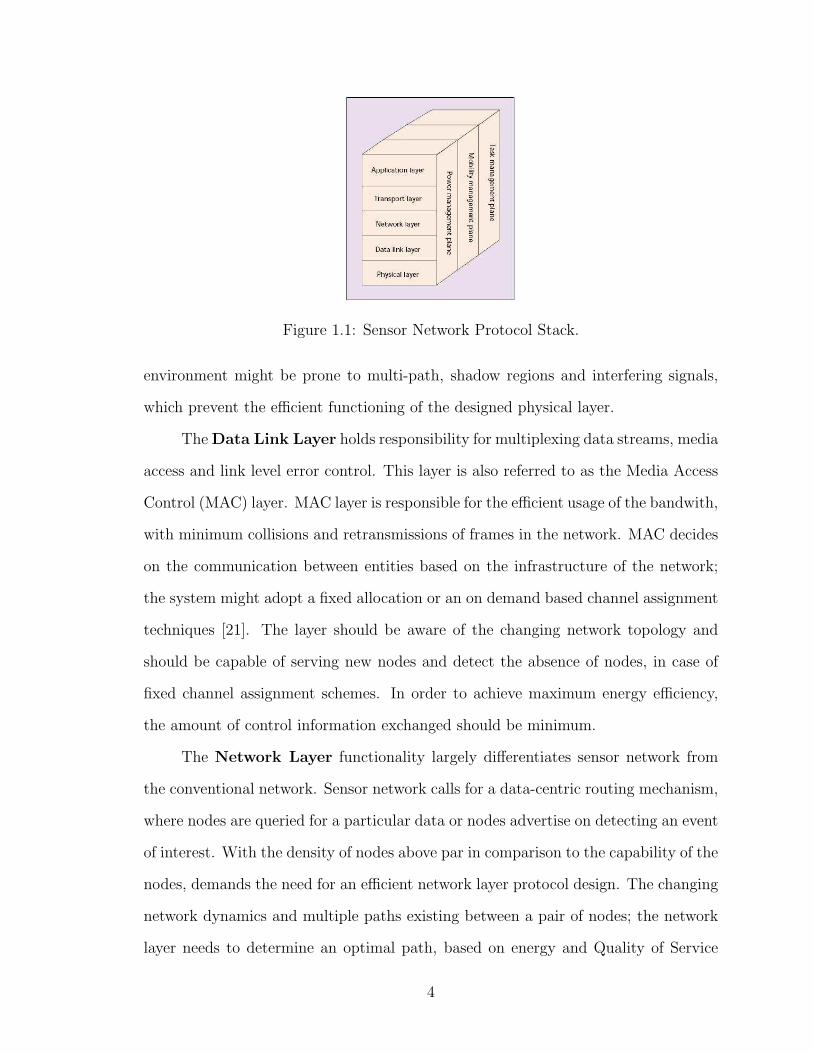
Figure 1.1: Sensor Network Protocol Stack.
environment might be prone to multi-path, shadow regions and interfering signals,
which prevent the efficient functioning of the designed physical layer.
The Data Link Layer holds responsibility for multiplexing data streams, media
access and link level error control. This layer is also referred to as the Media Access
Control (MAC) layer. MAC layer is responsible for the efficient usage of the bandwith,
with minimum collisions and retransmissions of frames in the network. MAC decides
on the communication between entities based on the infrastructure of the network;
the system might adopt a fixed allocation or an on demand based channel assignment
techniques [21]. The layer should be aware of the changing network topology and
should be capable of serving new nodes and detect the absence of nodes, in case of
fixed channel assignment schemes. In order to achieve maximum energy efficiency,
the amount of control information exchanged should be minimum.
The Network Layer functionality largely differentiates sensor network from
the conventional network. Sensor network calls for a data-centric routing mechanism,
where nodes are queried for a particular data or nodes advertise on detecting an event
of interest. With the density of nodes above par in comparison to the capability of the
nodes, demands the need for an efficient network layer protocol design. The changing
network dynamics and multiple paths existing between a pair of nodes; the network
layer needs to determine an optimal path, based on energy and Quality of Service
4
(QoS) metrics as desired by the application. Moreover, with the dense deployment of
sensor nodes ranging from a few hundreds to thousands, an addressing scheme would
add to the overhead, thereby forcing a network layer design without an addressing
scheme for nodes.
The Transport Layer is one of the less researched areas in sensor network,
this is because of the data-centric communication system which does not need an
efficient transport layer. The transport layer guarantees end to end communication,
but in sensor network the concern of every node is in transmitting it to the next hop
neighbor and does not follow an end-to-end data delivery model. Transport layer is of
growing importance with the integration of sensor network to the IP based network
or Internet. Currently, User Datagram Protocol (UDP) is used for sensor networks,
since it contributes less overhead compared to Transmission Control Protocol (TCP).
The Application Layer, based on information available from the sensor mod-
ule, advertises sensed data or reports events to querying nodes. The application
layer’s concern is in delivering useful information interpreted from the sensors raw
signals. The application layer is built to support the information delivery mecha-
nism opted by the sensor network, broadcasting information as and when detected
to neighbor nodes or reporting events on interest messages received from a central
node. The application layer can be supported by intelligence in prioritizing informa-
tion based on the sensor output or taking remedial action as in the case of sensor
cum actuator networks. Sensor Management Protocol (SMP), Task Assignment and
Data Advertisement Protocol (TADAP) and Sensor Query and Data Dissemination
Protocol (SQDDP) are a few protocols which have been proposed for the Application
layer.
The emphasis in this thesis is towards the design of a network layer protocol for
wireless sensor networks and the following section detail’s the design criteria’s and
challenges to be considered in designing a network layer protocol for sensor networks
5

1.3 Challenges in Routing Protocol Design for Sen-
sor Networks
Sensor networks are designed towards a specific application and different architectures
have been proposed catering to the needs of a specific application. Though the design
challenges for sensor networks would not vary drastically based on application but the
priorities of the design issues would vary based on the application. Sensor network’s
constraints and goals are different from contemporary wireless network design issues,
thereby forcing development of new paradigms. In this section some of the design
challenges are highlighted with their influence on routing information through a sensor
network.
1.3.1 Energy Efficiency
Energy is one of the prime factors to be considered while designing protocols for sensor
networks. Energy determines the sensor network’s lifetime; defined as the time taken
for the first node to fail due to energy depletion. On the sensor node hardware, the
development of CMOS technologies has reduced the size and energy consumption in
the modules; shifting the energy efficiency paradigm on the development of efficient
protocols. The communication circuitry consumes the maximum power compared to
all other modules on the sensor node. An efficient protocol design is to have minimum
message exchanges, both data and control messages. The transmission power on the
wireless channel is proportional to the square of the propagation distance, resorting
to multi-hop techniques would be energy efficient compared to direct communication
reaching far off distances. In most sensor network platform design, the battery has
a large form factor compared to other modules; thus reducing energy consumption,
would result in smaller battery modules and would further reduce the form factor of
the sensor node.
6

1.3.2 Network Dynamics
The changing network topology affects the path of data routing. During the initial
setup phase of sensor network, random deployment of nodes would result in non-
uniform node densities and multiple paths to reach a destination node; an optimal
routing path needs to be determined. Mobility of the sensor nodes drastically affects
the route stability and necessitates periodic route discovery. Mobility would lead to
bottle necks in the network, resting the connectivity of the network on few strategi-
cally located nodes. Apart from the nodes the dynamic nature of the sensed event,
target tracking application, would demand dynamic path setup and periodic routing,
demanding efficient routing mechanism.
1.3.3 Scalability
The number of nodes deployed vary, from a few hundred to thousand nodes, depending
on the application or the area of coverage. With no specific addressing scheme or
identification for sensor nodes, the routing protocol should be capable of routing
without relevance to an addressing scheme. An optimal routing protocol design should
be capable of operating over large number of nodes with not much depreciation in
performance with increasing number of nodes.
1.3.4 Data Aggregation
Most routing protocols designed for sensor networks are multi-hop and with large
number of nodes sensing identical events, a data aggregation mechanism would help
reduce redundancy and amount of information transmitted over the radio, thereby
saving energy. However, data aggregation should not degrade the performance of
the network. Data fusion process would result in nodes waiting for information from
7

neighboring nodes and delay in information delivery to the intended node. Protocols
need to tradeoff between aggregation and latency based on nature of the application.
1.3.5 Node Capabilities and Task Balancing
All sensor nodes are designed to perform the basic functionalities of sensing, process-
ing, communicating and relaying information. However, it is not necessary that every
node needs to be perform all the operations or identical operations at the same time
and each process consumes different energy. Nodes in close spatial proximity can co-
ordinate and balance work among themselves. As an example, one node could sense,
one other could relay and another node could be a data aggregation node, wherein
all nodes are in close vicinity. Nodes alternate between sleep and wake cycles and
uniform energy drain among nodes would be ideal. This is to avoid hot spots in the
network; meaning all nodes in a certain spatial location have failed leaving a hole in
the region being sensed. Also, task balancing helps in achieving increased network
lifetime.
1.3.6 Quality of Service (QoS) Requirements
The primary focus on routing protocol design has been in achieving energy efficiency
and increased network lifetime. However, the quality of data cannot be compromised
in certain critical applications, though energy is also of prime importance in those
applications. Sensor networks do not have a definite path for an end-to-end delivery,
but the QoS focus is on an end-to-end delivery in the present setup with minimum
time delay and bandwidth, yet retaining the energy efficiency paradigm.
8

1.4 Contribution
This thesis work details on a cross layer routing strategy for wireless sensor networks;
proposed a network layer protocol where in the application layer information and the
capabilities of the physical layer influence the network layer decisions. The protocol
considers volume of data has an important criterion for determining the next hop
node and suggests switching transmitter power levels as an energy efficient strategy
for routing packets. The thesis also suggests a method of switching OFF unintended
receivers based on the radio signal strength at the receiver end. The thesis is aimed
at increasing the lifetime of the wireless sensor network and reducing the end-to-end
delay in delivering the data, from the proposed algorithm.
1.5 Thesis Outline
Chapter 1 was aimed on introducing sensor networks and the network layer for sen-
sor networks, also outlined the design challenges for an efficient routing protocol for
sensor networks. Chapter 2 presents a literature review of existing routing protocols
developed for sensor networks, with an insight into the pros and cons of each protocol.
Chapter 3 details the proposed algorithm, arriving at a cost function and differenti-
ated service, based on the volume of the data to be routed. Chapter 4 details on the
implementation of the protocol in ns2, an event simulator. Chapter 5 draws a com-
parison of the proposed protocol with the existing protocol and results are analyzed.
Chapters 6 concludes with the authors contribution towards the thesis and further
scope of development.
9

Chapter 2
Routing Protocols for Wireless
Sensor Networks - A Review
With innumerable applications of wireless sensor networks and limited in terms of
energy availability, computational power and wireless connectivity; a number of pro-
tocols have been proposed specific to a genre of applications with optimal usage of
available resources. One of the main objective in designing protocols was towards an
extended network life time and also satisfying the design challenges, as detailed in
the previous chapter. This chapter classifies routing protocols, followed by an elabo-
rate discussion on the routing algorithms and current research focus in the design of
efficient routing mechanisms [6], [4].
2.1 Classification of Routing Protocols
Several routing protocols have been proposed with different priorities on the design
requirements and focus towards varied applications. This section is attempted on
grouping protocols into a common genre based on their behavioral characteristics.
In general, routing protocols can be classified as Proactive or Reactive, based
on the time the routing decisions are made. In proactive routing mechanisms, the
10

network paths are devised on sensor deployment, irrespective of a sensed event or
data availability for routing. As in the case of reactive routing, route path setup
is triggered by an event. Reactive protocols have the disadvantage of a delayed
information delivery since the routing decisions are triggered by events, but energy
efficient compared to that of proactive, wherein active paths are maintained even in
the absence of an event or data.
Routing protocols for wireless sensor networks can also be classified as flat multi-
hop, hierarchial and location-based, a classification based on the communication ar-
chitecture or interaction between sensor nodes. Flat multi-hop routing, a localized
approach with communication restricted within neighbor nodes and distant neighbors
are reached through multiple hops. In a flat schema all nodes are assumed to have the
same functionality. In contrast to the flat schema, the hierarchial approach supports
heterogeneity both in terms of node resources and functionality. Hierarchial routing
model is a cluster based approach, wherein nodes in the neighborhood directly com-
municate to a more capable central node. Location based protocols are an extension
to the cluster based approach, wherein the sensor nodes in a geographical region group
and interact. This class of sensor network nodes are capable of identifying themselves
in terms of location based attributes.
One other method of classification is based on the data aggregation capability of
the nodes. While routing information, nodes fuse their data with that of the neighbors
data before being routed, without processing the data. These protocols are referred to
as Non-Coherent Routing protocols. Coherent Routing protocols process the data and
fuse data before relaying, to the next hop node, thereby reducing data redundancy.
Coherent protocols also have the advantage of reduced transmission overhead.
Routing protocols can also be classified as Push or Pull protocols, classified
on how data is disseminated in the sensor network. In Push protocols the sensor
nodes on identifying an event advertise it throughout the network. In the case of Pull
11

protocols, user queries through the sensor network for information. Protocols may be
Pull or Push based on the application the sensor network is deployed.
Most of the routing protocols proposed for sensor networks had energy efficiency
and network lifetime as their performance measures. Adding on to these measures,
applications required guaranteed data delivery models, such protocols where in gen-
eral labeled Quality of Service(QoS) Aware protocols. The protocols addressed the
issues of an end-to-end guaranteed data delivery, latency in acknowledging the data
from the network, prioritizing the data and supporting real time data streams.
2.2 Routing Techniques
Having discussed on the grouping of sensor network protocols, this section details
on individual protocols grouped as multi-hop, cluster based, location based and QoS
aware routing techniques. Prior to the design of routing algorithms specifically for sen-
sor networks, Flooding and Gossiping where the two classical methods of routing
data through a sensor network. Flooding is a simple broadcast mechanism, wherein
each sensor node broadcast received packet to its neighbors. The process continues
until the packet reaches the destination or the maximum hop count of the packet is
reached. In gossiping, a node picks up a neighbor in random and forwards the packet.
Flooding has drawbacks of implosion, a node receiving multiple copies of the same
data and has no consideration for energy utilized. Gossiping avoids the problem of
implosion but adds to the delay in the packet reaching the destination and also there
is a probability of nodes not receiving the data packet.
2.2.1 Multi-hop Routing Protocols
This subsection details routing protocols that use multiple paths rather than a single
hop to reach the destination. The inherent advantage of these protocols is that they
12

need not know the nodes other than their neighbor nodes. These set of protocols have
a high fault tolerance as they are aware of or have a choice of multiple paths to reach
a destination. Nodes periodically acknowledge the presence of their neighbors, which
is an energy consuming process. However, the extent of neighborhood information a
node maintains and the number of alternate paths setup by a node is protocol specific.
Sensor Protocols for Information via Negotiation(SPIN), a reactive
push protocol [35]. SPIN compiled sensor nodes disseminate information as meta-
data (short, high level descriptors of the sensed event) to other nodes in the network.
Interested nodes on receiving the meta-data information query the node for more
information or the data, as illustrated in fig. 2.1 [35]. SPIN protocol acknowledges
the fact that neighbors do have the same information and distribute meta-data to far
off nodes. SPIN protocol implements data exchange through three messages; ADV
to advertise meta-data, REQ request for actual data on receiving the meta-data,
DATA message the actual information. The semantics of the meta-data are applica-
tion specific. The working group of SPIN proposed a family of SPIN protocols suiting
varied network topologies and energy aware schemes. Adding on to the basic SPIN
protocol, a family of SPIN protocols where proposed viewing energy awareness and
network topologies. SPIN-2 nodes incorporated an energy threshold scheme, nodes
below a set threshold would not participate in the meta-data cycle and would only
sense for events. Other protocols of the SPIN family [20] are SPIN-BC, for broadcast
channels, SPIN-PP for point to point communication (multi-hop), SPIN-EC for en-
ergy aware point to point communication and SPIN-RL accounting for lossy channel
characteristics.
SPIN has advantages over flooding and gossiping by reducing redundancy in the
information being transmitted and turns out to be energy conserving. However, SPIN
can be viewed as a process of controlled flooding, relaying meta-data to nodes that
would never require it, a source of energy drain. If the source and the destinations
13

Figure 2.1: SPIN Protocol: (a) meta-data advertisement from A to B (b) Node Brequests for DATA (c) Node A replies to B with DATA (d),(e),(f) the process repeatsfrom Node B to its neighbors
nodes are farther apart all the intermediate nodes maintain state and information
about the data being delivered across end entities. The meta-data mechanism does
not guarantee data delivery to distant nodes, intermediate nodes might not find the
information useful and may not advertise to its neighbors, resulting in events not being
reported to the sink nodes. However, SPIN has the advantage of being localized to
topological changes, since they maintain information on only there one hop neighbor.
The concept of meta data helps in querying data at any node for relevant information
on the network, rather than flooding interest to the network in search of events. SPIN
turns out to be an adaptive and reliable data dissemination model.
Directed Diffusion a query based, on demand PULL protocol [11]. Directed
diffusion supports a naming scheme for data identification and data is identified by
an attribute value pair. Sensor node, referred to as the sink, query the sensor net-
work with information of interest identified by a set of attributes and the interest
message is propagated through the network, a controlled flooding mechanism. The
propagated interest message are cached at all sensor nodes for a short time stamp.
Sensor nodes with matching data attributes respond to the interest message, these
nodes are referred to as the source nodes, illustrated in fig 2.2. Directed diffusion
14

Figure 2.2: Directed Diffusion (a) Interest Propagation Phase (b) Gradient SetupPhase (c)Data Dessimination Phase.
operates in three phases, the interest propagation phase, followed by gradient setup
phase and information dissemination phase. Gradients are setup for relaying back
information to the sink node. The final phase of data dissemination, wherein paths
are reinforcement and data is delivered from source to sink along the path estab-
lished with the help of gradients. Path reinforcement also aids in data aggregation
and setting up routes for further information querying and dissemination. The di-
rected diffusion discussed is refereed to as the Two Phase Pull Diffusion, turns out
to have lot of information exchange and inefficient for applications where in many
interest are diffused through the sensor network. Two other variants of directed dif-
fusion have been proposed [14] suiting various applications, the Push Diffusion and
the One Phase Pull Diffusion. Push diffusion was designed to overcome the problem
of maintaining gradients in applications, wherein information disseminated from the
network is low and maintaining gradients is expensive in terms of energy. In push
diffusion, the functionality of the source and the sink are reversed, the sink node
becomes passive and source becomes active and publishes exploratory data messages.
Gradients are established and paths are reinforced by exploratory data to the sink,
avoiding the process of setting up interest gradients as in the case of two phase pull
diffusion. When the exploratory data reaches the sink, reinforcement messages are
sent back to the source, setting up gradients, followed by data on the gradient path
to the sink. One Phase Pull Diffusion turns out to be more energy efficient than
Push Diffusion, wherein data are sent to sink along preferred gradients identified by
15

neighboring nodes minimum latency path. Neither interest reinforcement messages
nor exploratory data messages are sent out in this schema.
Directed diffusion and SPIN were the first few protocols addressed specifically
for sensor networks and had contrasting methods of information dissemination. Di-
rected diffusion turned out to be more application oriented due to the attribute nam-
ing characteristics of the sensor network. Directed Diffusion has the advantages of
restricting to local topology dependence and the inherent data aggregation capability
is highly energy efficient. The attribute matching at the nodes requires comparatively
higher intelligence at the sensor nodes incorporating directed diffusion. Since interests
are cached for short time interval, periodically interest needs to be broadcasted into
the network. On the other hand, caching interest for a long period of time questions
the buffer requirements at the sensor nodes. Directed diffusion is one of the successful
routing protocols for sensor Networks and many real world functioning models have
incorporated directed diffusion as there routing technique. Also, most routing proto-
cols are designed on top of directed diffusion and compared with directed diffusion as
a bench mark for performance.
Rumor Routing [7], identified as conservative flooding or a restricted diffusion
mechanism. Rumor routing is a variant of directed diffusion and finds application
where geographic routing mechanism is not feasible. The idea is to flood data to
those nodes that have detected a similar event of interest rather than flooding the
entire network. Event is flooded to other nodes with the help of long lived packets,
called agents. When a node senses a event, stores it in its local event table, and
generates an agent which carries event information to distant nodes in the network.
Nodes on receiving an agent store the information on their event table and the agents
path serve as reinforced path for routing information. Nodes respond to query based
on the information stored in the event table.
16
Rumor routing outperforms directed diffusion with limited flooding, however
rumor routing suits applications wherein the information through the network is less
and the number of events is less. With higher number of events reported the mem-
ory buffer on the sensor nodes would be a limiting factor. The protocol agent based
scheme limits only a single path of communication between the source and destina-
tion, as opposed to directed diffusion. Rumor route results in additional overhead
associated in maintaining the state of the agent and the event tables.
Energy Aware Routing Network survivability or elongated network lifetime
was the major design goal while sketching this protocol [32]. The protocol high-
lights the fact that solely relying on optimal paths would exhaust the nodes along the
path and depreciate the network lifetime; highlighting the employment of suboptimal
paths for routing. Each node maintains a list of paths to reach a particular destina-
tion with a probability measure based on an energy metric. The node chooses a path
for transmission based on the probability distribution. The protocol has three phases
of operation, the initial setup or interest propagation phase wherein localized flooding
takes place to associate an energy metric for all the paths. The energy metric cost
function is based on the transmission and reception energy and the residual energy
in every node. The second phase - data communication phase, paths chosen from
the node’s forwarding table based on the probabilities. The final phase -route main-
tenance phase, localized flooding to maintain and acknowledge live paths between
nodes.
Built over the directed diffusion paradigm with the notion of network survivabil-
ity, the protocol was proven to be energy conserving compared to directed diffusion.
However, the list of paths that needs to be maintained on the nodes demands greater
capability from the sensor nodes. Though proved to be energy saving the setup and
maintenance phase consume a lot of energy. The network is proven to be effective
over a limited number of nodes, its efficiency and memory requirements would be
17

questionable with larger number of nodes. Also increased protocol complexity, as the
number of paths to be maintained and the number of nodes in the sensor network
increase.
Gradient Based Routing (GBR) [31] a variant of directed diffusion wherein
the focus is on data fusion and uniform traffic distribution through the network for
optimal routing. When interest is diffused through the network, the hop count of
the message is acknowledged and incremented at every node. Each node discovers
the minimum number of hops required to reach a particular node. The hop count is
referred to as the height of the node. The difference between the node’s height and
that of its neighbor is considered as gradient of the link. Node forwards packet on
the link with the highest gradient. The paper details three data spreading techniques
for uniform traffic distribution. Stochastic scheme, the node chooses to route to the
next neighboring node randomly, when neighboring nodes have the same gradient.
Energy based scheme, when a nodes energy falls below a threshold, it increases its
height so that other sensors are discouraged from sending data to that node. Stream
based scheme, nodes routing a stream of data increase their height thereby diverting
new stream of data through other nodes.
The protocol is proved to have communication energy saving compared to that
of directed diffusion. This can be attributed to the focus on data aggregation and uni-
form traffic distribution schemes. Data aggregation reduces the overhead in compar-
ison to transmitting individual entities, effectively reduces the quantum of data com-
municated. Moreover, uniform traffic distribution splits the load evenly among nodes
in neighborhood, energy consumption is also uniformly distributed among nodes, sim-
ilar to the above discussed protocol. These factors attribute to the increased lifetime
of the network.
18

ACtive QUery based forwarding In sensoR nEtworks (ACQUIRE), a
data centric, distributed query based routing protocol [27]. The sensor network is
seen as distributed data base and capable of answering complex queries, consisting
of sub queries. A complex query is routed to a node in the sensor network, the node
answers the sub queries based on the pre-cached information available at that node.
Nodes unable to answer all the queries, forwards the query to the next node within
’d’ hop counts. Where ’d’ is referred as the look ahead parameter, which limits on
the number of hop counts in handing over the query to the next node. When ’d’ is
large then the routing protocol would simulate flooding with smaller values of ’d’ the
query would have to hop among larger number of nodes. A mathematical model has
been proposed to find out the optimal value of ’d’, which was found out to be four.
However, at a point when the query has been fully answered the node returns the
packet to the central node along the reverse path or the shortest path. The basis of
handing the query to the next node is random.
This process of iterative querying turns out to be energy efficient, but the delay
incurred in solving a query would be high and does not suit time critical applications.
If the query has been handed over to nodes far-off from the location where the event
has been sensed, the protocol adds to the delay in solving the query. A knowledge
of geographic aware routing or intelligently routing to nodes based on a probabilistic
model or prior information exchange from the nodes, would fasten the process of
querying.
Information Driven Sensor Query (IDSQ) and Constrained Anisotropic
Diffusion Routing (CADR) [25], the protocol is based on an information utility
measure on selecting which sensor to query and to dynamically route data. The infor-
mation utility measure is a mathematical quantification of the amount of information
gain that can be obtained by accessing a sensor node. IDSQ, works on selecting the
optimal node to query while CADR defines on how to query a node and routing to
19

the particular node. IDSQ works on electing a leader node among a group of nodes
and the leader node has knowledge of the position of the sensors. This grouping of
nodes with a leader node does not categorize this protocol as a cluster based routing
scheme, since this is just a virtual group for co-ordination among nodes for infor-
mation exchange, with no implication on the routing mechanism. The leader node
establishes a belief state for every node in its cluster; based on the information it can
process from the nodes. The belief state is function of the information utility mea-
sure, also depending on the application and the computational power of the node. If
the belief state is satisfactory then the node is queried; if the belief state is not satis-
factory the leader selects another node based on its position and information utility
measure. The leader node updates the belief state of a node on every query to the
node until a sufficient belief state has been reached. CADR, based on the decisions
made by IDSQ device route path to the sensors. CADR resembles directed diffusion,
with routing decisions made with or without the knowledge of position of the sensors.
If the location of the sensors are know, route is addressed to the sensor, arriving at
an optimal solution. The optimal solution is based on the evaluation of a composite
objective function; a cost function on information transfer utility, depends on query-
ing, routing, bandwidth and latency. In absence of information on the position of
the sensor, local decisions are made at every node satisfying a composite objective
function.
The protocol set maximizes information gain, with minimum latency and band-
width. The algorithm was proven to be more energy efficient compared to directed
diffusion, at the cost of increased protocol complexity. The protocol differentiates
itself from existing protocols by considering information gain along with communi-
cation cost parameters. The computational complexity associated with the protocol
raises high requirements on the nodes capability.
20
COUGAR, a data-centric protocol [39] views the sensor network as a dis-
tributed database system, using declarative queries to abstract information from the
network. Declarative queries meaning query states what to look for in the network
and not concerned on how to look for the data in the network. A query optimizer
generates an efficient query plan for in-network query processing based on the users
query. The author proposes an abstract query layer between the application and
network layer to serve the purpose of efficient querying. The queries generated are
independent of the network layer. COUGAR implements in-network data aggrega-
tion whereby one node is selected as the leader node which performs aggregation and
transmits the data to the central node. The central node generates a query plan,
which details the data flow, in-network data aggregation mechanism and selecting an
optimal leader node, which in turn is processed at the query layer of the sensor nodes.
COUGAR’s in-network aggregation reduces the overhead and ensures energy
efficiency on transmission of aggregated information. Introducing a new abstract layer
would turn out to be burdensome on the resource constrained nodes and adds extra
overhead on the node in terms of energy consumption and storage capability. The
process of in-network data aggregation from several nodes requires synchronization
between nodes and relaying nodes wait for packets from neighboring nodes, before
sending data to the leader node. Leader nodes are dynamically selected considering
energy availability on the nodes.
2.2.2 Cluster Based Routing Protocols
The process of creating clusters and cluster head contribute to the overall system
scalability, lifetime and energy efficiency. It supports heterogeneous sensor network
by allowing powerful nodes to perform energy consuming tasks and the other nodes
simply serve the purpose of sensing. The data delivery is in two stages, nodes com-
municate with a cluster head and the cluster head in turn needs to communicate
21
with the base station. The cluster based architecture demands heavy functionality
from the cluster head and the nodes highly rely on the cluster head. In heterogenous
networks with failure of cluster heads, the nodes might turn out to be useless with
no link to communicate with the base. In the case of homogenous sensor network,
any node might be elected as the cluster head, also nodes alternate as cluster heads
for even power drain among all nodes in the network. This subsection details a few
hierarchial cluster-based algorithms.
Low Energy Adaptive Clustering Hierarchy (LEACH) cluster based en-
ergy efficient data aggregation mechanism; functioning as a self organizing adaptive
dynamic protocol [36]. Nodes in spacial proximity group to form a cluster with one
of them opted as a cluster head. Nodes directly communicate within the cluster to
the cluster head, information within a cluster is aggregated at the cluster head and
then the cluster head transmits a single aggregated message to the central node. On
random intervals new cluster heads are elected and nodes join cluster heads in close
spatial proximity. The periodic change in cluster head is for uniform energy dissipa-
tion among nodes in the sensor network. Within a cluster communication follows a
Time Division Multiple Access (TDMA) schema, nodes communicate to the head at
periodic time slots. The setting up of LEACH is a two phase operation, the setup
phase and the steady state phase. The setup phase is when the clusters are organized
and actual data transfer takes place at the steady state phase. The duration of the
steady state phase is longer than the setup phase. The selection of the Cluster head
is based on a probabilistic model, where each node opt itself as the cluster head and
broadcasts it over the radio. Based on the received signal power nodes identify the
closest head and join the network.
LEACH, the first of its kind, emphasizing grouping as an energy efficient tech-
nique, but limiting itself to a specific applications. The direct communication between
the cluster head and the base is energy consuming. There is a possibility of a formation
22

of hole in the network, wherein a node might not hear a cluster head’s advertisement;
also the possibility of two many cluster head’s in close vicinity, as the decisions are on
an independent basis. The cluster head communicates to the central node using Code
Division Multiple Access (CDMA) technique. This demands the nodes participating
in LEACH to be highly capable supporting two different Network, Medium Access
Control (MAC) and Physical layers. The idea of cluster formation brings in overhead
in communication and synchronization needs between the cluster head and the nodes
belonging to the cluster. The protocol also assumes that all cluster heads consume
the same amount of energy, which is not true, energy consumption varies on the lo-
cation of the cluster head and number of nodes in the cluster. LEACH would not
suit for sensor network deployment over large areas since the distance between the
cluster head and central node would be far off for certain extreme nodes, demanding
more energy for transmission, this in turn might result in faster energy drain in dis-
tant nodes. LEACH was found to be efficient and said to have an extended lifetime
compared to that of SPIN and directed diffusion.
Power Efficient GAthering using Sensor Information System (PEGA-
SIS) and Hierarchial PEGASIS, a data aggregation protocol wherein neighboring
nodes communicate to form a chain link for the sole purpose of data fusion. Nodes
exchange information only with their closest neighbor, node’s sense closest neighbor
based on the radio power and adjusts it radio power to reach the closest neighbor
only. The formation of chain links is a greedy algorithm with nodes grouping to form
a cluster head, the construction of chain starts from the farthest node within a clus-
ter, since they have the least choice of neighbors. As a chain is formed and a node is
fixed to co-operate with a neighbor, the setup process shall never be revisited until a
neighbor dies. The chain link formed is the basis for data aggregation mechanism, the
cluster head broadcasts to the base station and the nodes within a cluster alternate
to act as cluster head, resulting in an uniform energy drain within nodes in a cluster.
23

The protocol was found to be energy efficient than LEACH. PEGASIS [22] aimed
at an extended lifetime for the nodes, thereby increased the overall network lifetime,
doubled in comparison with LEACH. The inherent disadvantage of this system is
the excessive delay involved in data aggregation, which turns down PEGASIS from
time critical applications. PEGASIS had an advantage of reduced communication
overhead in comparision with LEACH.
Hierarchial PEGASIS [29] was proposed to overcome the delay involved in the
PEGASIS model. The protocol proposed a shift from sequential data acquisition
as in PEGASIS to a simultaneous data aggregation technique. Pairs of nodes in
close proximity can communicate simulataneosly among themselves without causing
disturbance. Pairs of nodes communicate and one of them inturn communincate
with another node, this communication results in a tree hierarchy as shown in the
fig 2.3 [29]. A protocol supported a CDMA scheme and a non-CDMA scheme of
communication. The CDMA scheme supported communication among large pairs of
nodes simultaneous and did not have any restrictions on the hierarchy level. The non-
CDMA version had a restriction on the number of nodes that would communicate
and limited to only three levels in the tree hierarchy. The hierarchial version had
achieved significant reduction in delay involved in data fusion. The CDMA version
had comparatively lesser delay than the non-CDMA version. The complexity of
the protocol grew higher compared to that of its parent, communication overhead
increased as the complexity of the topology increased and node failures needed to be
sorted out more intelligently.
Threshold sensitive Energy Efficient (TEEN) and Adaptive Threshold
sensitive Energy Efficient (APTEEN) Sensor Network Protocol, a hierar-
chial cluster based protocol responding to abnormality in measuring the attributes
based on predetermined thresholds. Nodes group to form a cluster with a cluster head,
similar to that of LEACH approach and cluster heads communicate on a multi-hop
24

Figure 2.3: PEGASIS and Hierarchial PEGASIS (a) Data aggregation in PEGASIS(b) Data aggregation in Hierarchial PEGASIS.
fashion as illustrated in Fig 2.4 [2]. The protocol can be grouped as a reactive protocol
as the nodes are responsive to events and data would be generated triggered by ab-
normality over thresholds. The algorithm works on two thresholds, a hard threshold
and a soft threshold. Once the cluster based network topology is setup the threshold
information is sent to the cluster heads, which in turn transmit to the nodes. When
the sensed attribute changes by the hard threshold, the node reports to its cluster
head. On sensing the hard threshold level, the next communication in the network
would take place only after the sensed attribute changes by the soft threshold.
The threshold mechanism orients the protocol to be application specific. The
soft threshold saves on the number of transmission that would have occurred when
there was no change in the sensed attribute. The TEEN [2] protocol simply follows
this threshold mechanism and achieves energy efficiency by reducing the number
of communications. The drawback of the TEEN protocol is that when the sensed
attributes remain unaltered no information is transmitted. This raises doubts on
the existence of the nodes, alive or dead. Moreover, this technique is not suitable
for end users wanting periodic updates on the sensed attributes. To overcome the
limitations posed by TEEN, APTEEN [24] was proposed where in periodic updates
of the sensed phenomenon are over the network. APTEEN turned out to be proactive
and compromised on the energy efficient data delivery model of TEEN. The reactive
25

Figure 2.4: Hierarchial Clustering
property of TEEN was restored in APTEEN by responding to the threshold changes
apart from periodic data delivery. TEEN and APTEEN turned out to be efficient for
time critical applications and better performers than LEACH. It is also evident that
TEEN is more energy efficient than APTEEN, absence of periodic data delivery in
TEEN. However, the serious limitations of the set of protocols is in their application
specific nature and setting up of multi-hop route among cluster heads, which change
over random time intervals.
Energy Aware Routing in Cluster Based Sensor Networks [26], a rout-
ing protocol for heterogenous sensor network. This is a proactive routing mechanism,
the cluster head is considered to be a powerful node, less constraint in terms of com-
putational power or energy availability compared to the other node in the network.
The cluster head also referred to as the gateway is aware of the location of all nodes
in the network. The sensors nodes operate in either of the four states based on the
instructions from the gateway node; sensing only, relaying only, sensing & relaying
and inactive state; the functionality of each state is evident from their names. The
gateway node decides on the route by instructing each node in the network to com-
municate with whom and when. The decisions are made to conserve energy based
26

on a cost function. The cost function relies on the communication cost, energy avail-
ability at the node, energy consumption rate, node relaying cost, node sensing cost,
maximum connections per relay, propagation delay and queuing cost. Node’s com-
municate in a TDMA scheme, node’s have a fixed assigned time slot for transmission
and reception in the network. The gateway communicate’s with other gateways and
with the central base station.
The protocol was found to outperform other clustering protocols in energy met-
rics, network life time; and also in quality metrics, throughput and end-to-end delay.
The route setup changes to accommodate the changing the network dynamics. The
performance of this protocol is reliable and efficient; but the bottleneck is the power-
ful gateway module. The deployment of these nodes need to be organized; on random
deployment nodes might be far apart from the gateway and would fail to be a part
of the network.
Self Organizing Protocol (SOP) [33], a hierarchial routing protocol for het-
erogenous sensor network; stationary and mobile sensor nodes. The protocol relies
on a set of fixed nodes, called routers, as the backbone of the sensor networks and
the rest of the fixed or mobile sensor nodes probe in the neighborhood in search of
router nodes; forwarding information to the router node. The routers in turn com-
municate among themselves and to the central querying base station. All sensing
nodes, mobile or stationary, are networked with the router to be a part of the sensor
network. The protocol supports an addressing scheme for identifying all nodes in the
network and all nodes in the network are addressed based on the router node they
are tied to. Mobile sensing modules report to the router in close spatial proximity.
The hierarchial network frame is organized in four phases; Discovery phase, each node
independently discovers its neighbors and fixes its maximum radius of data transmis-
sion. Organization phase, the node aggregates into a group and a hierarchy of group
is formed in the network. Each node gets an address and a routing table is computed
27

for every node in the network. Maintenance phase, nodes keep track of their stored
energy and periodically broadcast to their neighbors; nodes periodically update their
routing table and energy level information of their neighbor nodes. Finally, self reor-
ganization phase, nodes detect failures and changes are reflected on the routing table
of the nodes. In case of network partition due to node failures, group reorganizations
are performed.
The hierarchial routing protocol has the benefits of good network connectivity,
the addressing schemes help in querying individual nodes and energy saving by op-
erating only on a subset of nodes. The cost of maintaining network routing table is
minimum and broadcasting is less energy consuming due to the hierarchial structure of
the network. The disadvantage is in the long organization phase and re-organization
phase on a string of node failures. The protocol could be more efficient if it worked
in an on-demand reactive basis, since a considerable amount of energy is utilized in
maintaining the network while no event has occurred.
2.2.3 Location Aware Routing Protocols
Location aware routing protocols are also referred to as geometric or localized routing
protocols. The nodes are identified based on a coordinate system, could be based on
latitude/longitude or could be a user defined coordinate system. Global positioning
system’s (GPS) have been proposed to identify the system on a global scope, but its
feasibility and cost is questioned. Simple localization techniques, like triangulation,
have been employed which can be used to identify the position of a sensor node
relative to the position of neighbor node. The routing protocols proposed have taken
it for granted all nodes are position aware and feasible routing protocols have been
proposed.
Geographic Energy Aware Routing (GEAR) [37] protocol proposes the
use of geographic information for disseminating queries within a sensor network. The
28

protocol works on energy aware and geographically-informed neighborhood selection
heuristics to route packets towards a target destination. The protocol, acknowledged
as an extension of directed diffusion, limits interest dissemination to appropriate re-
gions. The energy efficiency paradigm is based on a set of cost function’s; learning
cost and estimated cost of reaching destination. The estimated cost is based on the
residual energy at a node and distance to destination. The learned cost is the esti-
mated cost of routing around a hole in the network. A hole occurs in the absence of
a neighbor closer to the target region than itself. The node needs to find a route to
get around the hole, the cost estimate is framed from the learned cost. In the ab-
sence of the hole, the learned cost equals the estimated cost and forwarding decisions
are based on the estimated cost. The learned cost is propagated one hop back for
reiterating route setup on the next packet. The protocol has a two phased operation;
forwarding packets to a target region and forwarding packets within a region, as in fig
2.5. Forwarding packets to a target region is based on the cost function and deter-
mining the next hop neighbor closest to the target region. Once at the target region,
forwarding packets within the region is through recursive geographic forwarding or
restrictive flooding within the region. If the region is wide spread or high density of
nodes, the region is split into sub regions, copies of the packet are created and are
forwarded to the target regions.
With knowledge of geographic information GEAR has achieved better efficiency
in comparison with directed diffusion. Also GEAR floods region faster by creating
copies of data. GEAR can be grouped as a cluster based protocol wherein nodes
belonging to a region form a cluster, but their operation is a multi-hop and non-
hierarchial unlike the general group of cluster based protocol. GEAR is considered
to be a development over GPSR, a protocol for adhoc wireless networks which used
geographical information for routing with no emphasis on energy metric.
29

Figure 2.5: GEAR: Recursive Geographic Forwarding
Geographic Adaptive Fidelity(GAF) a location based energy aware routing
protocol for wireless sensor networks though primarily designed for mobile ad-hoc
networks. GAF [38] works on dividing the network into virtual grids and nodes
identify themselves on the grid knowing their positions with the help of a global
positioning system (GPS). Within a grid nodes are identified identically and nodes
within a grid collaborate among themselves. Nodes within a grid elect one node to
stay awake over a certain period of time and nodes alternate within a grid. The node
awake acts as the cluster head reporting to the base station on happenings within the
grid and also controls the nodes in the network. GAF programmed nodes operate in
three states, as illustrated in fig 2.6 [38]; Discovery, Sleep and Active state. Nodes
periodically get into the discovery phase, during the discovery state the node’s look
for neighbors, new mobile nodes might have moved into the grid and existing nodes
might have died or moved to new grids. In the sleep state, the node is in the minimum
energy consumption state with only their sensing modules ON and all other modules
are switched OFF. Nodes are active when they act as the leader or when the nodes
within a grid have sensed an event. Nodes utilize maximum energy in the active state.
GAF supports multi-hop routing among clusters head in reaching the central base
station, this identifies the protocol as a hierarchial protocol.
30

(a) (b)
Figure 2.6: GAF(a)Virtual Grids in GAF (b)State Transitions in GAF
GAF shows an increase in network lifetime as the density of nodes within a
cluster increase. The fact that all nodes are identical within a grid and one node
awake all the time, ensures network connectivity and contributes to the extended
network lifetime. The high end assumption that all nodes identify themselves through
a GPS, might not fit all category of sensor network applications where cost of the
node is of great concern. Moreover, the power consumption on identifying nodes on
a GPS system is not accounted for energy consumption. The leader node does not
support any data aggregation or fusion mechanisms; this feature would have added
up towards the efficiency of the protocol. GAF inherently supports mobility and its
performance is comparable with ad-hoc networks in terms of latency and packet loss.
2.2.4 QoS Supportive Routing Protocols
In the above groups of routing protocols the emphasis was on energy efficiency and
focused on increased network lifetime, with little concern on quality measures. This
group of routing protocols in addition to the energy efficiency focus on QoS metrics
such as latency, bandwidth and efficiency. QoS based protocols emphasize on ac-
knowledging the data at the right time, differentiating data based on priorities and
propose reliable routing algorithms. The protocols are concerned on the network
fault tolerance and resilience of the network on node failures or node malfunctioning.
Based on QoS metrics a few protocols have been elaborated.
31

Sequential Assignment Routing (SAR) [18] one of the first QoS based
routing protocols for sensor networks. Routing decisions where made based on the
energy consumption along the path, QoS metrics, such as delay and bandwidth, and
priorities of each packet. A multi-path tree structure is formed from the source down
to every sink or base stations in the network; every node in the network is a part of
the tree structure. The network is resilient to node failures along a path as multiple
paths exist between a source and the base station. The paths are void of nodes with
low energy and unable to provide QoS guarantees. Each link in the path contributes
towards the end-to-end cost metric as measure of resistance to the packet flow through
that path; this information is used in framing an additive metric of the traffic flow
through that path. A weighted QoS metric is calculated as the product of the additive
QoS metric and a weighted coefficient associated with the priority of each packet. A
node failure causes automatic path restoration locally. For dynamic sensor networks
and to enforce path reliability, the base station initiates periodic re-computation of
the path thereby accommodating changes in the network.
SAR turned out to be more energy efficient than protocols that considered only
energy as a metric and ignored the priorities of packets. Having multiple paths be-
tween the source and the sink ensures guaranteed data delivery and fault tolerance.
However, the protocol suffers from excessive overhead of maintaining tables and state
at each sensor node especially when the number of nodes in the network is high.
A recovery procedure is enforced when a node fails locally and periodic path rein-
forcement, maintaining routing path consistency between upstream and downstream
nodes on each path. This proactive characteristics of the protocol turns out to be
an energy consuming procedure for the network which has not detected any event.
One nodes failure might result in a dramatic change in the network tree structure, as
traffic through a node is a cost function metric.
32

SPEED, a stateless, localized QoS based routing protocol with minimum over-
head and end-to-end guarantees. SPEED’s QoS metric is the ability to maintain a
desired delivery speed across the network, hence the name SPEED [34]. The protocol
maintains information about neighbors and geographic information of the nodes in
finding a quick route. The end-to-end delay estimate is made knowing the distance
between the source and sink and the speed of the packet before route decisions are
made at the nodes. Stateless Non-deterministic Geographic Forwarding Algorithm
(SNGF) is the main routing module of SPEED, works on choosing the next hop
nodes targeting a desired delivery speed and within a theoretical delay bound. SNGF
co-ordinates with four other modules in making routing decisions. Neighbor beacon
exchange module for periodic information exchange between nodes, gathering infor-
mation about the nodes and their location. The rate at which neighborhood beacons
are exchanged depends on the network dynamics; a static or slow moving nodes in
the sensor network would have a low beacon rate. SPEED employs a single hop delay
as a metric to approximate the load on the node. Assisted by the delay estimation
module, the time elapsed to receive an acknowledgement in response to a packet sent
to a neighbor gives the delay estimate. The delay estimated helps in selecting the next
hop node. If a decision could not be made with the delay estimate, Neighborhood
feedback loop module calculates the relay ratios of node. The relay ratio is calculated
with respect to the neighbors of the node which could not provide the desired speed
on earlier requests. The fourth module, Backpressure Rerouting module, alarms the
source if packets are dropped at nodes unable to find the next hop neighbor, thereby
initiating new routes at the source.
SPEED provides a reliable data delivery model with uniform speed for time
critical real-time applications. The protocol has information of its immediate neigh-
bors and does not maintain any routing table, thus described to be a stateless routing
protocol. SPEED’s congestion control mechanism dismissed the need for a QoS aware
33

MAC protocol. But this function of SPEED brushes off the advantages of a layered
protocol architecture, burdening the network layer with too many functionalities.
SPEED’s SNGF module achieves load balancing by relaying the traffic across differ-
ent paths, backing an energy efficient mechanism.
Maximum Life Time Routing in Wireless Sensor Networks [8], works on
formulating the routing issue as an optimization problem with the goal of maximizing
the sensor network lifetime; considering the fact that the communication circuitry
consumes the maximum power in routing and making use of nodes with maximum
residual energy for relaying information on the network. The protocol is intended
for identifying the traffic pattern in the network for routing. Two traffic patterns
are considered, fixed information generation and arbitrary information generation;
and a flow augmentation algorithm is proposed which iteratively augments the flow
along the shortest cost path. The routing issue is formulated as a linear programming
problem, solvable in polynomial time. The objective was to find the best link cost
function to maximize the network lifetime. The parameters that were considered for
calculating the cost over the link are energy expenditure for unit data transmission
over the link, the initial energy before transmission and the residual energy on the
nodes. Importance is given to the residual energy in the node on transmission rather
than the shortest path or minimum energy path. The least cost path solution is
formulated using Bellman-Ford Algorithm, whose residual energy is largest among all
paths.
The protocol emphasizes on the residual energy for increased lifetime compared
to algorithms which considered the minimum transmission energy and the shortest
path for routing. The tradeoff is the computational complexity in solving for the best
cost path.
34

Maximum Life Time Data Gathering and Aggregation in Wireless
Sensor Networks, the protocol [19] maximizes the network lifetime by information
gathering and aggregation mechanisms. The QoS aware protocol works on maximizing
the life time of the network as data gathering problem and is presented as polynomial
time algorithm. The protocol defines network life time as the number of periodic
data readings taken from the sensor before a node in the network fails. The proposed
method solves the maximum lifetime data gathering problem for sensor networks,
where in-network data aggregation is possible. The solution is in an optimal data
gathering for routing data to the sink. The route path is a multi-hop tree structure
from the source to the sink, and the schedule is followed for a designated time, called
the system life time. The protocol aims in maximizing the system life thereby avoiding
frequent change in schedules. The problem is formulated as a flow problem with linear
objective functions and linear constraints. The linear objective function is computed
over a polynomial time and a solution of real integer values is obtained. In the case
where in-network data aggregation is not possible, for video streaming applications,
then the problem is modeled as a network flow problem and energy constraints on
the sensor also considered, arriving at a similar solution as in data aggregation case.
The protocol design increased the lifetime of the sensor network in comparison
with hierarchial PEGASIS. However, the delay in delivering the data was greater
compared to that of Hierarchial PEGASIS, this can be attributed to the data ag-
gregation mechanism involving nodes along the route waiting for every other nodes
data for information fusion. The computational complexity of the network is high for
practical implementation in a constrained Wireless Sensor Network module.
Minimum Cost Forwarding Protocol [13], a simple and scalable protocol
aimed at finding the minimum cost path in a large sensor network. A back-off timer
based cost function algorithm that finds the optimal cost for data transfer from any
node to the sink node with one single message overhead at each node. The cost
35

function captures the effect of delay, throughput and energy consumption from any
node to the sink. The protocol operates in two phases, in the first phase the cost
values are calculated at every node. The calculation of cost starts from the sink
message diffused to all nodes. Every node calculates its cost as a function of the cost
of the node it received the message from and the cost of the link. The cost at every
node is calculated based on a back-off based algorithm, every node on receiving a
message backs-off and waits over a certain period of time to receive the minimum
cost message. Then the node broadcasts only a single message to its neighbors with
the minimum cost. In the second phase, the source broadcasts data to its neighbors.
The nodes on receiving the broadcast message subtracts its transmission cost to the
cost of the packet. If the remaining cost of the packet is not sufficient for forwarding
the packet to the sink, the packet is dropped at that node else the packet is forwarded
to its next set of neighbors.
The protocol does not remember the next hop neighbor node or its address
for communication, as all cost function calculations are done independently at every
node. Generally, cost field calculations are done by flooding the network, but has the
inherent disadvantage of excessive advertisement messages as the node is unaware of
the least cost path until receives all the packets. The back-off timer concept helps in
overcoming the problem by delaying the broadcast until the node is sure of having
received the least cost path message. Simulation results have proven that cost function
calculated using flooding and back-off timer yield the same results, but the later has
achieved the same with minimum advertisement messages. Nodes not maintaining
information on their next hop neighbor ensures scalability of the protocol. The time
for which the nodes defers transmission is critical and the back-off algorithm sets the
deferral time proportional to the optimal cost at a node.
Energy Aware QoS Routing [3] a class-based routing protocol supporting
differentiated service for real-time and non real-time traffic. The protocol finds the
36

least-cost, energy efficient path for data in terms of the link cost calculated based
on nodes energy reserve, transmission energy, error rate and certain communication
parameters. The class based queuing model is as shown in Fig. 2.7 [3] , wherein
each node has a classifier and differentiates the realtime and non realtime traffic,
servicing them through different queues. There is a scheduler which determines the
order of the packets to be transmitted from the queues based on the bandwidth
ratio ’r’. The bandwidth ratio is the initial value set by the gateway and represents
the bandwidth allocation ratio to real time and non-real time traffic. The classes
can borrow bandwidth from each other when either of the traffic types are non-
existent or within limits. The queueing delay for the traffic is found with the help of
the ’r’ parameter. The cost function calculation takes place in two stages, first the
candidate least cost paths are found and selects one that meets the end-to-end delay.
An extended version of Dijkstra’s algorithm is used in ascending the set of least cost
path.
The protocol is consistent with respect to QoS and energy metrics. The as-
signment of ’r’ value was uniformly set for all nodes, which does not provide flexible
bandwidth sharing for different links. A later version of the protocol supported differ-
ent values of ’r’ for different links. The protocol supports both best effort and realtime
traffic at the same time; best effort by means of the cost path and differentiation in
bandwidth for real and non-real time traffic.
2.3 Open Issues in Sensor Network Routing
The inherent characteristic of sensor network is to operate in large numbers on several
constraints yet yield satisfactory results. Many routing protocols for various applica-
tions, prioritize a few and trade-off a few constraints based on the application. A lot
37

Figure 2.7: Queuing model for Energy Aware QoS Routing
more domains in this field are unexplored or await optimal solution, a few of them
are identified and listed below.
• The protocols discussed in this chapter suited applications where the data was a
few bytes of information. With end sensors like cameras wherein the information
generated is large, the path meant for small data sizes is used for large data sets
too, is this an efficient way is an unexplored area. The research focus would be
to justify differentiated service for information based on the data size and find
an optimal path, the present thesis focuses on this topic.
• The sensor network modules are being foreseen to be used by humans in ev-
eryday life. This calls for the integration of sensor network with the present
IP based network or Wide Area Network (WAN). The focus is on developing a
suitable architecture for networks to co-exist, retaining their functional charac-
teristics.
• Nodes can collaboratively process and compute data, and reduce the amount of
data communicated over the radio resulting in significant energy conservation
on the nodes. The concept here is synonymous with grid computing, wherein
a group of nodes share the computation burden, apart from data fusion mech-
anisms.
38

• Sensor nodes are deployed in random location and require a GPS to identify
themselves in a global space. The GPS system can operate only in open spaces,
also expensive and energy consuming for establishing its position. The alterna-
tive is the development of localized algorithm identifying itself with respective
to its neighbor nodes and knowing the position of one node on the global space,
one should be capable of mapping all the nodes on to the global space. Also
using localized algorithm a new co-ordination system can be developed rather
using the existing infrastructure.
• Sensor networks being applied in various military applications monitoring and
collecting sensitive data, securing the data is of great importance. In sensor
network an end-to-end security model is not of interest, as neighboring nodes
would require access to the information. Current work has been on neighboring
nodes acknowledging their true presence and nodes capable of distinguishing
between friends and foe in a remote spatial distribution of sensor nodes.
39

Chapter 3
A Cross-Layer Routing Protocol
for Wireless Sensor Networks
Having reviewed prevalent routing protocols for wireless sensor network in the pre-
vious chapter; wherein the emphasis was in arriving at efficient routing decisions
banking on a set of network parameters; without comprising on the message that
needs to be routed and focused on energy utilization. Decisions where made inde-
pendent of other layers in the sensor network protocol stack, except that all layered
protocols shared the knowledge of the energy availability on the sensor node in com-
mon. Apart from the network layer, the concept of energy efficiency was addressed
in the application layer of wireless sensor networks for collaborative information pro-
cessing and distributive task management; the Medium Access Control layer dealt
with efficient channel allocation, synchronization and management of ON and OFF
duty cycle’s; and power control algorithms for energy efficient physical layer design.
The layer specific protocols were optimized individually for best performance and
eventually all layers addressed issues for extended sensor network lifetime. Evidently
working towards a common goal, collaborative functioning and unified effort would
help achieve better efficiency [30]. As detailed in [30], information from lower layers
40

would help higher layer protocols function more efficiently and towards better usage of
network resources. A cross layer protocol design helps achieve better performance by
optimizing for an efficient co-existence in the protocol stack. The proposed network
layer protocol, a cross layer design, is acquainted with application level information
influencing routing decisions by tapping on the physical layer capabilities of the sensor
node.
Real time low cost sensor modules, often referred to as motes in the sensor net-
work community, are devices with limited capabilities and energy resources, designed
to operate in large numbers in a networked fashion. The current generation of these
motes developed for sensing applications such as the MicaZ, TelosB, Sun SPOT’s and
the Intel mote’s physical layer are compliant with an IEEE 802.15.4 standard for the
physical layer. The IEEE 802.15 group works towards the standardization of Wireless
Personal Area Networks (WPAN) or short range wireless networks; one among them
is IEEE 802.15.4 standard for low data-rate and long term battery operable sensor
networks. In the current work, the proposed protocol relies on the capabilities of the
802.15.4 transceiver and details an energy efficient routing strategy, influenced by the
volume of data thats needs to be routed and the energy availability in the nodes. The
succeeding section in this chapter details on the pros and cons of a cross layer design,
citing recent research on the cross layer design for sensor networks. The subsequent
section details on the IEEE 802.15.4 physical layer specifications. The proposed cross
layer routing protocol(XLRP) is elaborated in section 3.3, and finally in section 3.4
the factors influencing the decision making process are elaborated.
41

3.1 Cross-Layer Design for WSN
The concept of layered protocol architecture helped lay down a functional framework,
wherein each layer had a well defined functionality and service definition, working in-
dependent of the other protocols in the stack. The model eased complex network
design, supported heterogenous networked systems and inter-operable standard in-
terfaces were designed. However, the layered architecture was best suited for general
wired or wireless networks, wherein the Quality of Service(QoS) and inter-operability
was of prime importance, however in wireless sensor networks the emphasis is towards
energy efficiency and optimal usage of network resources. Moreover, sensor networks
being application specific and built to serve a specific purpose, protocol design can
be customized towards an application scenario. In line with this fact, cross layer
protocols were proposed for wireless sensor networks [5, 9, 23, 28], wherein the layer
functionalities are grouped to form a single entity.
Driven by the need for a cross layer design for efficient routing, in [23] and
[28] the MAC layer and the network layer were unified. In [5], a resource efficient
unified protocol was proposed combining the functionalities of all the layers into a
single protocol, a complete alternative to traditional layered protocol architecture;
the design complexity of the protocol increased as the number of factors influencing
a decision making process was large; nevertheless the protocol proved to be efficient,
in terms of energy and throughput. In [23], the lifetime of the sensor network was
extended by uniting the functionalities of the network layer onto the MAC layer
capabilities. The MAC layer organizes the network into a set of active and passive
nodes, establishing connectivity through outthe network on a TDMA( Time Division
Multiple Access) based scheme. The TDMA works on a multi-hop fashion, with
nodes establishing connectivity with their neighbors based on the local information,
setting up synchronized talk cycles; apparently shifting the route formation burden
from the network layer to the MAC layer. The network route path is set through
42

the connected system of active nodes, greatly relying on the information of the MAC
layer; However, a small time sync disturbance in the MAC scheme or the death of an
active node, would require the re-synchronization of the entire network, and need to
devise new routes; the penalty of over dependence on the MAC layer.
In [28], efficient cross layer routing is achieved by combining the MAC function-
ality based on the routing decisions made at the network layer, reducing the overhead
involved for medium access. The route path is setup by a stateless routing mecha-
nism at the receiver node rather than the sender node, resulting in receiver contention
rather than the sender contending to send information. The mechanism is based on
geographic routing and is an end-to-end decision making process, between the origin
node and the final destination node, making the protocol computationally complex as
most protocols designed for sensor networks are based on localized information at the
node. CoLaNet [9], an cross layer design of energy efficient wireless sensor networks,
worked on collaborating on the characteristics and requirements of the application
layer with the network layer in forming a route tree and the MAC layer scheduling
algorithm. The network tree is based on data gathering from many to one sensors and
the MAC was a TDMA based channel assignment algorithm. As discussed for [23],
the problem of adaptability of the network to changing network dynamics because of
a TDMA based media access.
The radio being one of the most energy consuming modules in the sensor node
is predominantly controlled by the MAC layer, deciding on the radios ON/OFF cycle.
When a sensor network is deployed the MAC is always active, irrespective of data
being sensed keeps the network connected, however the above layers are reactive and
act only on sensing events. The active state of MAC is unavoidable in the case of
multi-hop sensor network for effective data communication across the network. And
MAC functionality being software controlled, increasing the functionality of MAC by
clubbing on network layer functionalities would tend to drain more energy when no
43

event is being sensed, as suggest in above cross layer protocols. The cross layer routing
protocol dealt with in this thesis, operates independent of the MAC layer but enhances
power management, in addition to the MAC functionality, by controlling the radio
modules based on application level information. Moreover, XLRP though relying on
the information from the application and physical layer operates independent of the
layer specifications and functionalities.
3.2 The 802.15.4/ZigBee Physical Layer
The IEEE 802.15.4 standard , a Wireless Personal Area Network (WPAN) Standard,
proposed for low cost self-organizing mesh networks, especially for applications de-
manding low data rates and low power consumption. ZigBee is a multi-vendor consor-
tium, an industry alliance for manufacturing IEEE 802.15.4 compliant radio modules.
The standard operates in the Industrial, Scientific and Medical(ISM) band, 2450 MHz
and the 915/868 MHz band, and supports a maximum data-rate of 250 kbps. The
objective of the standard was towards a design of a reliable, short range communi-
cation interface with minimum operating cost and relaxed throughput requirements,
ideally suited for sensor network applications. The 802.15.4 standard details the
MAC and the Physical layer specifications, defining simple message exchange formats
and operating characteristics for the transmitter and the receiver. Currently a few
802.15.4 compliant radio modules are being manufactured, Chipcon’s CC2420 is a
widely used 802.15.4 compliant radio module which is being integrated into Berkeley
(Micaz, Telosb) and Intel motes. The proposed algorithm is simulated in NS2 with
Chipcon’s CC2420 radio module specifications, as a reference model for the physical
layer. However, using a manufacturer specific data-sheet does not confine the working
of the algorithm to the specific product; only that relying on a real-time radio model
44

aids in accurate energy modeling of the system and utilizing those parameters helps
in prototyping real time scenarios through simulations.
The CC2420 is a single chip programmable 802.15.4 compliant radio module
operating in the 2.4 GHz unlicensed ISM band. The transceiver is operable at low
voltage levels of 2.1 - 3.6 Volts and are low current consuming devices, with a receiver
sensitivity of -90 dbm the current consumed is 18.8 mA and for transmission at the
maximum power level of 0 dbm is 17.4 mA, the transmitter is capable of switching
eight power levels from -25 to 0 dBm. The transmitter power switching capabilities is
of significant importance for sensor nodes operating in large numbers, as this feature
confines interference to smaller regions when multiple nodes would need to commu-
nicate at the same time and also giving the flexibility to communicate with relatively
distant nodes. CC2420 is a Direct Sequence Spread Spectrum Transceiver supporting
a data rate of 250 kbps modulated using O-QPSK (Orthogonal-Quadrature Phase
Shift Keying) technique.
The transmitter and the receiver capabilities are of significant importance for
the proposed cross-layer routing mechanism. Reiterating the fact that transceiver
operation are the most energy expensive functions in the sensor network and with
network layer dependence, the knowledge of energy consumption in each of the radio
states is of prime importance. Capable of operating in five different states, the Idle
state with oscillator ON is the when the receiver circuitry is ON and sensing the
channel, when radio signals are detected it triggers receiver hardware functional and
is in the higher power consuming receive state. The difference in current consumption
between the Idle state with oscillator OFF and power down state is because of the
voltage regulator, the voltage regulator is turned OFF in the latter state and thereby
the entire radio module is powered down. Table 3.1 details the current consumed in
each of the radio states, the energy is calculated with knowledge of the supply voltage
and the time period for which the radio is ON.
45

Radio state Max. Current ConsumptionTransmitting at 0 dbm 17.4 mAReceiving 19.7 mAIdle Mode, Oscillator ON 365 µAIdle Mode, Oscillator OFF 20 µAPower Down Mode 1 µA
Table 3.1: Radio States and their current consumption.
Transmitter Power (dBm) Current Consumption (mA)0 17.4-1 16.5-3 15.2-5 13.9-7 12.5-10 11.2-15 9.9-25 8.5
Table 3.2: Radio Transmitter Power Levels and the current drawn.
The radio module is powered by a 3 volt supply, the product of voltage and
current gives the power; times the period the radio is ON in a particular state gives
the energy consumed over the time interval. Table 3.2 lists the eight transmission
states as per the 802.15.4 standard specifications and the current consumption in the
corresponding states is tabled for the CC2420 module. In the present case of WPAN
communication modules, the radio operations consumes few tens of micro amps for
transmitting and receiving and the maximum transmitting powers being 0 dBm,
draining only a few micro amps; thereby the energy consumed in switching between
radio states is appreciable. As in [17], the author has calculated the energy consumed
in switching from one state to another for the CC2420 radio module, the information is
reproduced in table 3.3 for switching between eights levels of transmitting, receiving
and idle states. From the data presented, the protocol iterates that for short transmit
or receive cycles, the energy consumed in switching is of concern and of significant
importance in determining the cost of the communication.
46

Transition Energy Con-sumption(µJoules)
Transition Energy Con-sumption(µJoules)
Rx - Tx(0dBm) 6.92 Tx(0dBm) - Rx 6.16Rx - Tx(-1dBm) 6.62 Tx(-1dBm) - Rx 6.13Rx - Tx(-3dBm) 6.31 Tx(-3dBm) - Rx 6.14Rx - Tx(-5dBm) 5.90 Tx(-5dBm) - Rx 6.08Rx - Tx(-7dBm) 5.53 Tx(-7dBm) - Rx 6.02Rx - Tx(-10dBm) 4.94 Tx(-10dBm) - Rx 5.95Rx - Tx(-15dBm) 4.16 Tx(-15dBm) - Rx 5.82Rx - Tx(-25dBm) 3.77 Tx(-25dBm) - Rx 5.70Idle - Tx(0dBm) 3.13 Idle - Tx(-10dBm) 2.52Idle - Tx(-1dBm) 2.99 Idle - Tx(-15dBm) 2.39Idle - Tx(-3dBm) 2.90 Idle - Tx(-25dBm) 2.24Idle - Tx(-5dBm) 2.73 Idle - Rx 5.92Idle - Tx(-7dBm) 2.67 Rx - Idle 3.35
Table 3.3: Radio Transmit and Receive Transition Energy Consumption.
3.3 The Cross-layer Routing Protocol (XLRP)
One of the characteristic feature that distinguishes wireless sensor network from an
Ad-Hoc Network, is the knowledge of information that would be generated in the
network. Sensor networks being deployed for a specific application, one is aware of
the information that would be generated from the sensor and the volume of data the
sensor network would render, based on the sensors in the network. As an example, a
temperature sensor would give out one or two bytes of data, an acoustic sensor would
generate a few hundred bytes, an image sensor would generate images of few kilobytes
of information; and also in the case of a heterogenous sensor networks the volume of
information that would be generated can be scaled. The XLRP algorithm explores
an efficient routing strategy based on the volume of data exchanged in the network.
The protocol relies on the fact that any information transmitted from source to sink
(destination) is complete when received in its entirety; as the process of transmission
may involve fragmenting the data into packets based on the maximum transmission
units supported by the network.
47

On the physical layer, sensor node radio modules are programmed to operate
at low transmitting power reaching their closet neighbor causing less interference,
aspiring for minimum energy drain and extended network lifetime. In general, sensor
nodes switch to higher transmitting powers to reach farther nodes, where in the im-
portance is in rendering information of high priority with minimum latency; a tradeoff
between energy and latency. However, the current protocol establishes the fact that
resorting to low transmitter power levels is not always the energy efficient strategy.
The proposed routing algorithm corroborates on switching transmission power levels
based on the volume of the data being transmitted as an energy conserving mecha-
nism for protracted network lifetime. Supported by the fact that for smaller volume
of data, the transmitter is on for a shorter period, so transmitting at low power levels
would be more efficient in comparison to switching power levels at the expense of
energy consumed. However, for larger volume of data the transmitter would need to
transmit for a relatively longer time, and the energy consumed in switching to higher
transmitter power level would be negligible, moreover hoping over a few intermediate
nodes would save on energy and reduced delay. Nevertheless, transmitting at high
power levels results in increased transmission radius and increase in the number of
unintended receivers, eventually resulting in an energy drain. The proposed XLRP
algorithm saves energy by switching OFF unintended receivers based on the power
of the received radio signal. Also, the routing decision are based on the energy avail-
ability, the local communication cost and node connectivity, the details of which are
elaborated in the subsequent section. Though XLRP nodes are capable of switch-
ing transmission powers, nodes are interested in information about their immediate
neighbors, meaning neighbor nodes that can be reached with the least transmission
power level, for decision making process.
In most energy aware routing protocols and were neighborhood information is of
importance, nodes exchange beacon messages with their neighbor nodes in a periodic
48
fashion. Though the neighbor messages are broadcasted only when active subscrip-
tions are present, energy is drained during this process. The proposed XLRP protocol
is suggestive for reduced energy consumption by piggy backing node information on
its transmissions and also evokes unintended receivers who had received the packet
to process and extract information from the received data. For example consider a
random distribution of nodes as shown in Fig. 3.1, for the highlighted node in the
center the radius of transmission with the least power level is the highlighted region,
the highlighted node is interested on the energy levels of the nodes within the region.
Also, any node communicating within this region would be heard by the nodes within
its transmission, thereby nodes on receiving the packets, process the header to find if
it was addressed to it and the packets are dropped, as in any conventional network.
However, XLRP is suggestive of nodes process the packet to extract information about
the sender node if it is within its region of interest, neighborhood table. Iterating the
fact that receiving consumes lot more energy than processing, and thereby extract
information from the received information rather than dropping the packet after re-
ceiving, however do not react (respond) to the received packet. This methods saves
energy by avoiding periodic beacon messages for marking neighbor node presence. In
XLRP, nodes broadcast information identifying themselves to their neighbor nodes at
different operational transmitter power levels and also respond to new identification
messages received from new neighbor node, with a set delay between identification
messages being transmitted.
3.4 Criterions for Routing Decision
This section details the controlling and contributing factors in determining the next
hop neighbor, enroute for communication through the wireless sensor network.
49

Figure 3.1: Node and its neighborhood region of interest
3.4.1 Switching Transmission based on Volume of Data
Information disseminated though the network vary from a simple interest message
or sensor data; to a control or an acknowledgement/reinforcement message. Apart
from the messages being unique in functionality; the messages can be classified by
their size in terms of the number of bytes. This application layer information, size of
the data, made available at the network level helps determines the next hop neighbor
and accordingly switches the transmit power level at the physical level. As stated in
the previous section, most sensor deployments and algorithms prefer operating the
radio transmitter in the minimum power level state to avoid interference, reducing the
burden on the MAC layer design. However, the current proposed algorithm tries to
explore the energy saving possibilities in switch transmitting powers based on the size
of the data, moreover, it adds to the MAC layer functionality of switching radio states
and conserving energy. The XLRP switches to high transmission power levels for large
volume of data and remains in lower power levels for small packet transmission. Larger
packet size implies larger transmission and reception time, meaning the radio is in
high power consumption state for a longer time. Transmission of a larger packet at low
transmitter power levels results in an increase in number of hops, delayed reception
and multiple nodes draining minimal energy but collectively energy consumed would
be higher; whereas switching to higher transmitter levels reduce the number of hops
and reduced delay in data reaching the destination. However, an individual node
50

would have drained lot more energy than it would have if transmitted at lower power
levels. Nevertheless, the collective energy drain would be less as we have reduced
the number of transmitter and if only we could reduce the number of unintended
receivers, detailed in the subsequent section. Moreover, this does not exhaust the
energy reserve on a single node, has energy in the node is also considered in decision
making process.
Also in sensor networks, the setting up of path and routing is more towards
circuit switching than packet switching, unlike in conventional wireless networks; as
maintaining multiple paths for routing is at the cost of a node’s energy. When a
few kilobytes of information needs to be routed between two nodes, the information
is broken into packets and the route path is established to transmit these packets
through a single established path, rather than sending through multiple paths. an
increased burden of sequencing the packets at the receiver end and expensive in terms
of energy in maintaining multiple paths. Thereby switching to higher transmit state
and switching off intermediate nodes from receiving would help reduce the number of
transmission and receptions.
3.4.2 Signal Strength based Decision Making
The CC2420 radio module has the capability of measuring the signal strength of
the received radio signals. This feature has been explored in localization algorithms
in determining near and far neighbors, wherein nodes are programmed to operate at
fixed power levels and based on the received signal strength the proximity of the sensor
nodes can be determined, modeling the propagation losses. With nodes capable of
operating at different power levels and knowledge of the received signal, the proposed
model conceptualizes on a back-off mechanism for unintended receiver nodes to switch
their radio modules, saving on energy.
51

The number of unintended receivers increase on switching to higher transmission
power levels, nevertheless they can be limited by switching of the receiver based on
the received signal strength. For example, if a node wants to talk to distant node
it would switch to a higher transmitter power level sufficient for the desired node
to receive (the transmitter node has prior knowledge of the required transmission
power level); meaning the signal strength of the receiver node would be close to the
radio modules receive threshold. Also nodes within the transmission range of the
sender would receive the signal, however the signal strength of the node adjacent to
the transmitter node would be different from that received by a farther away node.
Truly the sender would not transmit at a very high power level to reach its adjacent
neighbor node, capable of being reached at a lesser transmitter power level and the
viceversa also holds true. Thereby, setting up a maximum signal strength threshold
value, receiver modules sensing signals above the set threshold consider themselves
unintentional receivers and turn OFF their radio modules. This is an iterative learning
process wherein nodes learn from messages received (during the neighbor discovery
phase) and set their threshold values.
A limitation on the effective functioning of this mechanism is the size of the
packets being transmitted. The process involves the radio module listening to the
radio signal, determining the signal strength of the received signal, then rendering
the value (RSSI) to the microcontroller module in the sensor node, which makes
the decision on turning OFF the receiver and finally switching OFF the receiver if
required. If the packets being transmitted is only a few bytes of data, the time taken
to make a decision and enforce it would be longer, for the packet would have been
received over the period; however, for lengthier packets this mechanism would be
effective in terms of energy conservation. The time involved in this process helps
determining if a message is short or long, and helps opting for the right power level.
52

This further restates the need for switching to higher power levels based on the volume
of the data that needs to be transmitted.
3.4.3 Energy in the Node
Energy availability in node is of great concern in determining the operations the node
would need to perform and also the overall network lifetime. The node functionality
is based on a relative measure of the energy with respect to its peer neighbor nodes.
Also, nodes with limited energy would not take part in energy expensive operations,
such has switching to higher transmission power levels and acting as relays for mul-
tihop communication. Restating the definition of network lifetime, the time taken
for the first node in the network to fail; an ideal protocol design would drain energy
uniformly among all the nodes, eventually leading to the death of all nodes at the
same time or near close intervals.
The strategy of switching to higher transmission power based on data volume
and switching OFF the radio to save on energy, as discussed in the above sections,
would not convince one on uniform energy drain among the nodes. However, decisions
planned on considering energy as a relative quantity and the circle of neighborhood
under consideration would connotate uniform energy drain. When a node transmits
at an higher power level, the nodes immediately surrounding the transmitting node
would turn off their radio sensing very high radio signals, assuming large packet
sizes transmissions, resulting in large difference in energy availability among neighbor
nodes. The measure of the difference in energy levels can be calculated as a ratio
of the nodes energy to the average energy of its neighbors. If the ratio is greater
than one implies that the node being considered is more resourceful compared to its
neighbors and less than one would push the node to operate in energy conserving
state; transmitting at lower transmitting power levels and excuse itself from network
route relay paths. The ratio would also vary based on the neighbor nodes being
53

considered, if the ratio is with respect to the first tier neighbors, meaning nodes that
can be reached with the least transmitting power; the energy ratio would vary even
for small difference in work load on nodes but more uniform energy drain, however
considering larger subset of neighbors would average out the high difference and lessen
the regulations on the node. XLRP algorithm restricts its neighborhood region to
nodes within its least transmission range.
3.4.4 Communication Cost
The communication cost parameter is analyzed in terms of the energy consumed by
the node for that specific radio communication. The cost calculation is based on the
energy availability, the energy consumed for the operation and the energy consumed
in switching nodes to the required states. In the case of large volume of messages to
be relayed by a node, the node needs to switch to higher power state, the decision to
choose a power level is based on the energy consumed for the node to transmit in that
state and what would be the energy ratio after the node as transmitted in that state
with respect to their neighbors current energy availability. As ideal energy ratio is
one, the decision made on selecting the particular energy state should’nt bring in large
changes to the energy ratio. For large messages, being transmitted as a sequence of
packets, nodes can switch to lower power states after transmitting a series of packets,
thereby avoiding any possible large variation in energy with that of its peer nodes.
This is suggestive of nodes changing network paths after a sequence of transmissions.
3.4.5 Node Connectivity
The position of the node relative to the nodes in the network is of prime importance in
deciding the node participation for efficient routing and extended network lifetime. In
scenarios were the density of the nodes is high, meaning a node has larger number of
neighbors to choose from, the nodes have high connectivity and the network load can
54

be effectively shared among the nodes. With lesser node density implies poor node
connectivity, the nodes functionality is seriously limited; as in worst cases scenario
the death of a few nodes might part the sensor network. The node connectivity
parameter would determine the functionalities of the node; with poor connectivity
the node would not switch to high transmitting powers and would be less engaged
as a relay node, excusing itself from energy depleting processes. The dependence
of node functionality on the node connectivity parameter can be attributed to the
collaborative functioning of sensor network and energy as a collective measure of a
region, and not just a nodes energy. In addition the node connectivity parameter
can be also be used to determine the next hop neighbor, data could be forwarded via
nodes which have a higher count of neighbors; in cases of two promising next hop
neighbors with equal energy levels or proximity to the final destination, the node with
higher connectivity would be a better choice.
Quality of Service for sensor networks can be categorized into Application spe-
cific and Network based QoS, as identified in [10]. The application specific QoS in
unique to sensor networks, which deals with sensing area coverage, exposure, posi-
tioning of sensors, functions of sensor and sensor measurements, details relevant and
specific to the application scenario [10]. The Network QoS is applicable for any net-
worked system, dealing with network resource allocation, service guarantees in terms
of delay, throughput, data delivery, to name a few; and for sensor networks all the
QoS guarantees are addressed in terms of energy consumption and efficient network
utilization. XLRP reduces the delay in message transmissions by switching to higher
transmission power levels. The application layer based switching characteristic of
XLRP would reduce the transmit/receive time by limiting the number of intermedi-
ate nodes along the route, reducing the delivery time from sender and receiver and
also saves on energy. Having identified strategies and constraints for efficient routing,
the proposed cross layer protocol is being implemented in Network Simulator (NS2),
55

detailed in the following chapter. The effectiveness of the protocol is being proved
though the simulations in comparison with that of directed diffusion implementation
in NS2.
56

Chapter 4
Implementation In Network
Simulator (NS2)
Having discussed the cross layer routing protocol in the previous chapter, this chapter
details on modeling of the proposed algorithm in network simulator. The first sub-
section details on the simulator, followed by the implementation details of directed
diffusion in the network simulator, which forms the basis of the current implementa-
tion. Section 4.3 details on the implementation of the proposed cross layer routing
in ns2. The final section details on the energy model in ns2 for calculating the energy
consumed during the routing process.
4.1 Introduction to Network Simulator
Network simulator(ns, better know as ns2) is a discrete, event simulator for model-
ing wired and wireless network scenarios. In the presented work, network simulator
version 2.29 is being used. The simulator is written in objected oriented C++, for
implementation of core algorithms and OTcl (object Tcl) shell scripts as a frontend
tool, for testing and simulating the performance of protocols implemented in C++
57

[1]. The C++ and OTcl have mirror implementations with an one-to-one correspon-
dence; network models are developed by creating instances in tcl (tool command
language) that are linked to the corresponding C++ object modules. C++ is used
for detailed protocol implementations has it provides a higher level of control and
flexibility on data handling, packet format and exchanges. Also, C++ executes faster
compared to that of tcl scripts, thereby reduced run time for complex algorithms
running over large data sets. On the other hand, tcl is easier to program and modify
compared to that of C++, thereby helpful in creating test scenarios and instances of
protocol implementations in C++ [1]. For example, both TCP (Transmission Con-
trol Protocol) and UDP (User Datagram Protocol) have implementations in c++,
however the choice of a node adopting TCP or UDP schema is opted at the tcl level.
Tcl helps design network topologies with nodes as the hardware entities in a network
and nodes are configured to a set of protocols as agents, representing the software
entities. Packets are the fundamental unit of data exchange between agents in the
simulator. The simulator supports protocol implementations for unicast, multicast
and broadcast packet exchanges.
All events in the simulator are queued based on time, a scheduler executes the
next earliest event in the queue, completes the current event execution before exe-
cuting the next event in queue, also adds event’s dynamically as a result of executed
events. The tcl interface allows user to schedule events. The results of simulation on
the execution of tcl scripts are in the form of trace files which detail on the various
events such as packet arrival, departure or packet drop. Every event in the trace file is
timed precisely to a nano second. The trace file can be formatted based on the fields of
interest, the file that needs to be modified is located at ns-2.29/trace/trace.{h,cc}. To
track events and generate trace files, a common header is included in every packet,
uniquely identifying the packet. The common header includes a set of field’s for
58

handling packets during simulation and are not accounted towards performance eval-
uation of protocols. Fig 4.1 is snapshot of a sample trace file, wherein the first row
indicates if a packet is being sent or received, represented by ’s’ and ’r’ respectively;
’D’ indicates a packet is dropped. The second column indicates the time in seconds
at which the event had occurred. The subsequent column indicates the node id, de-
fined in tcl scripts, followed by ’AGT’ indicating agent generated message, ’RTR’
indicating router or network layer generated message or ’MAC’ indicating message
generated by the media access layer. The next column, a long series of number, is
a unique identifier for every packet generated, this is a field in the common header;
followed by the word ’diffusion’ indicating the message is generated by the directed
diffusion agent. The subsequent field indicates the packet size, in the trace file snap-
shot packet size is displayed only for packets communicated over the radio, received
or sent by the MAC layer. The four values within the square braces, indicate the time
to send, source MAC address, destination MAC address and the packet type (ARP or
IP or AODV) in hexadecimal; however, these fields are not applicable to our current
simulation. The final column also enclosed within square braces are applicable for
IP based simulation, the first two pairs separated by semicolon indicate the source
IP address, source port address and destination IP address, destination port address.
The last two fields indicate the time to live (TTL) value of the packet and the next
hop node information, if any.
The network simulator does not support any GUI (Graphical User Interface),
however the simulator does support a visualization tool, nam (network animator);
helps picturise the network setup with nodes and node movements, if mobility en-
abled. Also, help visualize packet transfer between wired nodes and wireless node
transmissions with their region of coverage. To run nam, a specific nam trace file
needs to be generated while executing tcl scripts, nam trace file is different from the
trace file discussed earlier. The tool animates the network operations as timed events
59

Figure 4.1: Snapshot of a trace file
for the entire length of the simulation period; the time step can be changed with the
help of the controls provided on the GUI. Fig 4.2 is a snapshot of the nam GUI with
a few wireless nodes represented as black dots and the circles centered around a node
indicating the radio signal reach at that instant of time, if continued over time the
radio signals might propagate further or diminish. Nam tool is useful for visualizing
simple network scenarios with a few tens of nodes, however with a few hundred nodes
interpreting network activities in nam would be cumbersome.
4.2 Directed Diffusion
Directed diffusion was one of the first protocols for wireless sensor networks to be
implemented in ns2. The simulator supports all variations of directed diffusion, the
two-phase pull, one-phase pull, one-phase push(or simply push) and GEAR imple-
mentations. The control flow for directed diffusion implementation in NS2 is as
represented in Fig 4.3 [1]. The directed diffusion core(the core diffusion agent)
helps integrate the protocol into the network simulator suite, as a wrapper class for
sending and receiving packets to and from the network. The different variations of
60

Figure 4.2: Nam user interface
Figure 4.3: Message flow in Directed Diffusion (redrawn from [1])
61

directed diffusion are implemented as filters communicating with the core diffusion
agent. This has the advantage of testing diffusion algorithms individually or in com-
binations, for example GEAR implementation with two phase pull can be compared
with that of GEAR with push algorithm. The decision making process and the flow
of packets within directed diffusion is controlled by the core diffusion agent. Every
filter included in the current simulation has a predefined priority, a packet arriving
at the core agent is directed to the filter with the highest priority and subsequently
to filters with lower priorities. The core diffusion agent in addition to encapsulat-
ing diffusion packets in the NS2 module, stores information that are in common for
the apps and filters. The apps block in the figure provides interface for source and
sink applications, that invokes the publish and subscribe interfaces for interest dis-
semination and data exchange between nodes. All these modules have equivalent
tcl instances, the core agent needs to be initiated first by selecting the routing pro-
tocol as Directed Diffusion, and the diffusion algorithms are initiated as filters,
GradientFilter for the two phase algorithm and GeoRoutingFilter for invoking
the geographic routing algorithm in tcl scripts.
The diffusion header implemented in ns2 includes a twenty four byte constant
header and message attributes of varying length based on the message type. The first
field identifies the diffusion packet with a version number, if a packet other than the
specified version is received, the packet is dropped by the diffusion agent. Followed by
the message type field, identifying a beacon request, data, interest or a subscription
message. The next three fields are two bytes long identifying the source port, length
of the message and the number of attributes in the message. Diffusion also generates
a thirty two bit packet number for uniquely identifying every packet generated by the
diffusion layer and followed by a thirty two bit random id for every node; and the
last field indicates the address of the next hop node.
62
Attributes in directed diffusion are represented using attribute-value-operator
tuples; serves for comparing interest messages and specifying node properties such has
longitude, latitude and energy. Moreover, the tuples help in matching interest and
subscriptions using simple logical operations. For example, longitude, latitude, infor-
mation specific to node or sensor capabilities, like temperature form the attributes,
the values correspond to attribute type can be string, integer or float data type. Fi-
nally operator details on interpreting and comparing the attribute values, operators
are IS, GE (greater than or equal to), GT (greater than), LT, LE, to name a few. In
diffusion implementation every subscription and publisher message is identified by a
unique hexadecimal number, helps in associating subscriptions with a source node.
4.3 XLRP Implementation
The proposed cross layer routing protocol is being implemented in ns2 identical to
directed diffusion implementation in ns2. Initial implementation attempts where for
XLRP to be part of directed diffusion as one other filter, however the difference in
packet header information and the programming complexity in adding a protocol
as filter to directed diffusion led to the implementation of XLRP as a stand alone
module.
4.3.1 Message Types
The protocol implementation handles three different messages for communication
among node; subscription, data and identity messages. In our implementation the
publish message is local to node, a node is identified as a publisher by creating a
tcl instance and the message is local to the node created by the apps agent and not
broadcasted. The subscription message is an interest message broadcasted by sink
node to the network, includes an unique interest identity. When matching publication
63

identities exist a data message of varying size based on the interest is directed towards
the sink node.
Identity message’s are broadcasted by nodes during the initial setup phase,
when the node joins the network and also when a new node joins the neighborhood.
Initially, identity messages are transmitted at all power levels. When a new node
joins the neighborhood, the identity message is transmitted in the power level as
that of the new node’s transmission, this information is included in the node identity
message. The node identity message also includes the nodes current energy level.
One other instance when the node transmits its identity message is when the node
can no longer support relaying of messages and serves only the purpose of sensing in
the network. The message is not flooded as in the case of subscription and is intended
only for nodes within its neighborhood. This message is flooded locally, at the least
transmission power, within the region wherein the node information is present in the
receiver nodes neighborhood table. If the message is received by a node for which the
information is not useful, no entry in the neighborhood table, the packet is dropped
and message is not broadcasted any further.
The XLRP protocol switches transmitter power level based on the number of
bytes of information thats needs to be transmitted, which is applicable only to data
messages because of varying data volume based on the publisher (source) node infor-
mation. Node identity messages which are also transmitted at different transmitter
power levels but are not subjected to check on data size for choosing the power level.
In other words, the protocol’s check for switching power level is applicable only for
unicast data messages. As subscription messages are of minimal bytes and needs to
be broadcasted among all the nodes in the network, the power level for subscription
message is never switched. By default the transmitter operates at its least power
level.
64

4.3.2 Message Header
Figure 4.4 details the basic header format of the proposed XLRP algorithm. In
addition to the header information used in diffusion implementation XLRP relies on
few other parameters for its functioning. The first eight bit version field identifies
XLRP message, if message other than XLRP message arrives at the node the packet
is dropped. The second eight bit type field identifies the message as an identity, sub-
scription or data message. The two byte agent field is useful in routing information to
the appropriate agent, distinguishing between the filters and the application agent.
The header also includes a four byte randomly generated packet number uniquely
identifying the packet generated, this is in sync with the directed diffusion implemen-
tation. All nodes in the simulation are addressed by a two byte node id generated
in a random fashion, which is also a part of the header. Followed by the next hop
and the last hop node id’s which are also two bytes long. All the above mentioned
fields are also a part of the directed diffusion implementation. Energy of the current
node is also included in the header field, which is two bytes in length and length field
indicating the size of the packet in two bytes. Unlike the current implementation,
energy is broadcasted only in beacon messages of directed diffusion implementation
and represented as a tuple. Two other fields that have been included in the common
header is the current node’s transmitter power level and the node connectivity para-
meter. The transmitter power level as decided by the cross layer protocol is included
in the header, thereby the receiver would in turn know the transmission power level
to reach the transmitter node. In the neighborhood learning process this of great
importance since it determines the power level by which the neighbor node can be
reached, this is under the assumption that the channel is symmetric; meaning if a
node can reach another node with a specific transmission power level, the viceversa
is also true.
65
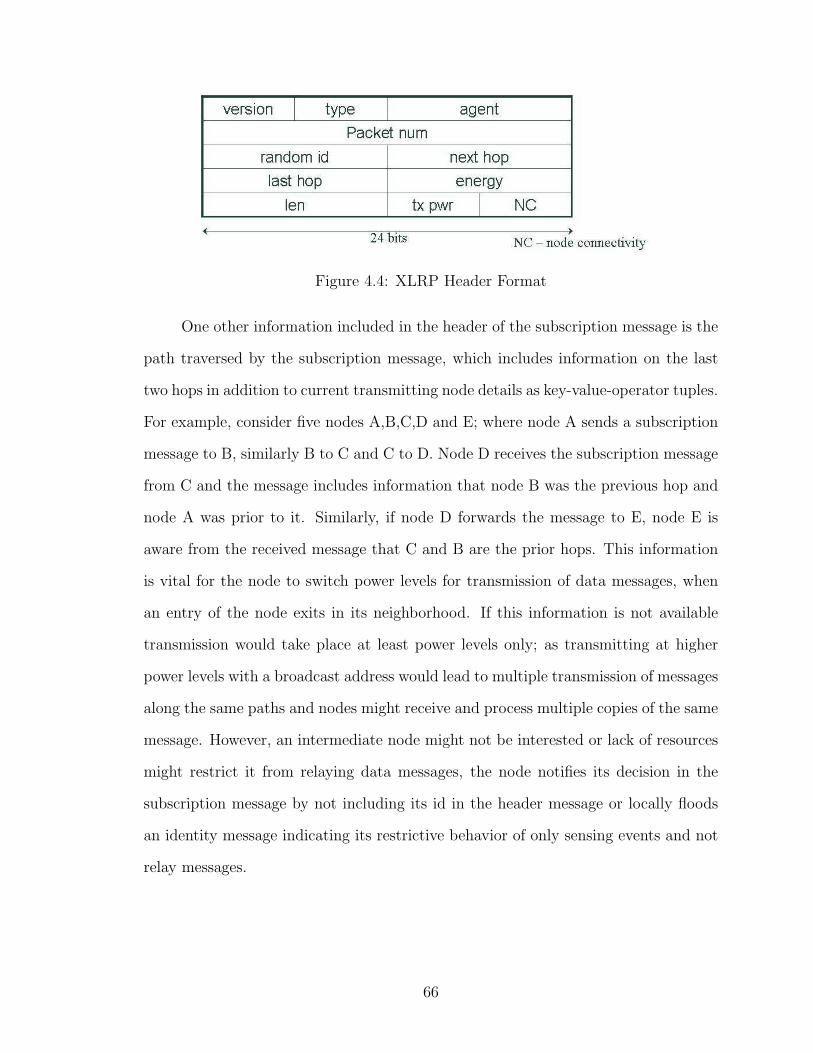
Figure 4.4: XLRP Header Format
One other information included in the header of the subscription message is the
path traversed by the subscription message, which includes information on the last
two hops in addition to current transmitting node details as key-value-operator tuples.
For example, consider five nodes A,B,C,D and E; where node A sends a subscription
message to B, similarly B to C and C to D. Node D receives the subscription message
from C and the message includes information that node B was the previous hop and
node A was prior to it. Similarly, if node D forwards the message to E, node E is
aware from the received message that C and B are the prior hops. This information
is vital for the node to switch power levels for transmission of data messages, when
an entry of the node exits in its neighborhood. If this information is not available
transmission would take place at least power levels only; as transmitting at higher
power levels with a broadcast address would lead to multiple transmission of messages
along the same paths and nodes might receive and process multiple copies of the same
message. However, an intermediate node might not be interested or lack of resources
might restrict it from relaying data messages, the node notifies its decision in the
subscription message by not including its id in the header message or locally floods
an identity message indicating its restrictive behavior of only sensing events and not
relay messages.
66

4.3.3 XLRP Phased Operation
The working of the XLRP protocol can be detailed as a three phase operation; Neigh-
bor Discovery Phase, Interest Dissemination Phase and Data Delivery Phase.
Neighbor Discovery phase is the initial phase of sensor network setup wherein
nodes broadcast their identity. For the first time when nodes are activated, they
broadcast their identity message at different operable transmitter power levels. Dur-
ing this phase nodes learn about their neighbor nodes and the power level the re-
spective nodes can be reached based on the header information. Nodes retransmit
identity message only when a new nodes join the network and the identity message is
transmitted at the power level required to reach the new node. Also identity messages
are broadcasted when there is an appreciable change in the energy level of the node
in comparison with neighbor nodes energy level. During which nodes advertise and
locally flood at the least transmitting power level and indicate that the node can only
sense indicated as a tuple attribute.
Interest Dissemination phase, the interest message is broadcasted at the least
transmitter power level and flooded through the network. In the interest dissemina-
tion phase apart from the common header, the last two hop information and the
interest id is also included in the message being broadcasted. The interest identifier
helps in reinforcing paths with minimum latency, based on the latency with which
the subscription messages are being received.
Data Delivery phase, occurs when an event is sensed and information is routed
from the sink node to the source node. Data messages are unicast messages, messages
are directed to the neighbor node with matching subscription. In a general IP based
wireless network data routing is an end to end model, wherein the sink node is aware
of the final destination node or the source node, however this is not the case in wireless
sensor networks, the sink node is only aware of the neighbor node it needs to direct
the data message and has no knowledge of the final destination node.
67

4.3.4 Physical Layer Characteristics
The zigbee radio module has discussed in the previous chapter, has the capability to
switch between eight different transmission power levels. However in the simulation
we are opting for three transmission power levels; as the emphasis in this thesis is to
implement the idea of routing by switching transmitter power levels for which three
power levels would be sufficient. The three transmitter power levels opted are -15,
-7 and 0 dBm and their corresponding transition energy measurements are taken to
account. The receiver sensitivity or receiver capture threshold has been opted as
-90dBm and the carrier sense threshold has been chosen to be -100 dBm. When the
received signal strength is within the receiver sensitivity limits then signal is captured
and can be decoded to receive the entire packet, however when the signal strength is
between the receiver capture threshold and the carrier sense threshold then a part of
the signal can be received and the packet cannot be decoded completely; equivalent
to packet not being received in simulation environment but the channel is busy for
transmission. The carrier sense threshold is used to sense if the channel is free before
attempting for transmission.
The RSSI (Received Signal Strength Indicator) is a part of the radio module,
a registry in the CC2420 radio module. The received signal strength is calculated
every eight symbol periods of the received signal strength. For the node to decide in
turning OFF the receiver or not it needs to communicate with the micro-controller, the
micro-controller compares it with the threshold value and turns of the receiver. The
process of switching OFF the radio module takes place in few tens of microseconds,
the entire operations is assumed to last for a few tens of milliseconds. In the current
simulation we have turned OFF the radio on satisfying two measures, if the receive
signal strength exceeds the software receive threshold as set by the network layer and
reception time exceeds the time required to receive the node identity message. This
aids in identification of new nodes joining the network.
68

Two ray ground propagation model is used in our simulation, wherein the re-
ceiver and transmitter antenna gain are set to one and frequency of operation is the
2.4GHz band at a transmission bandwidth of 250 kbps (kilobits per second).
4.4 Energy Modeling
Energy model in ns2 helps simulation of energy efficient protocols, by modeling the
energy consumption when the radio is in receive, transmit, sleep or idle mode’s. In
addition, the energy model accounts for energy consumption during transition from
idle to sleep mode and viceversa. The energy monitoring feature is implemented
as part of the wireless physical layer interface (ns-2.29/mac/wireless-phy.{h,cc}) and
accesses the energy model implementation at ns-2.29/mobile/energy-model.{h,cc}.The wireless physical layer simulates the transmission and reception of the packets
through the physical channel, thereby triggers energy calculations when there is a
change in the radio state. Also periodic energy calculations are initiated for nodes
which are in the sleep state. The energy model does not have information of the radio
states, but maintains information on the residual energy in the node and calculates
energy exhausted and residual energy based on the time and the power consumption
information provided by the wireless physical channel; the product of power in watts
and time in seconds is the measure of energy consumed in joules.
The wireless physical layer interface details on the transmitter power and re-
ceiver sensitivity. For the current implementation, decisions made at the network layer
are made available at the physical layer interface and also the physical layer data is
rendered to the network layer to aid in the decision making process. The transmit-
ter power level and the dynamic receive threshold set by the XLRP algorithm are
passed on to the physical layer. Based on the information received the transmitter
power level is switched and the packet is transmitted, corresponding transmission
69

energy and radio state transition energy calculations are triggered. Based on the re-
ceiver threshold information from the above layer, the radio is switched OFF and the
packet is dropped. Also, information on the signal strength for the received packet is
made available at the network layer, to aid in decision making processes.
The current energy model has been modified to accommodate the energy cal-
culation as required by the proposed cross layer routing protocol. In the original
energy model, transition energy between sleep and idle states where only accounted,
the same was extended for any state change in the radio model. As discussed in the
previous subsection, the common header is required for ns2 simulations and gener-
ation of trace files, moreover the common header is unique has the packet traverses
towards the various layers (application, network, mac and physical layers) of a node,
maintaining its unique identity. In the current implementation, the common header
is being used to share information across layers within a node.
The proposed cross layer routing protocol has been implemented in the network
simulator; with tcl instances for instantiating the core filter agent and the XLRP
filter, in similar grounds as that of the directed diffusion implementation. Also the
subscribe and publish instances have mirrored tcl instances. Various test scenarios
have been generated and the effectiveness of the protocol has been proven in the
subsequent chapter.
70

Chapter 5
Simulation Results and Discussions
The preceding chapter detailed on the protocol and the implementation of the algo-
rithm in network simulator. The current chapter demonstrates the efficiency of the
algorithm by simulating a wireless sensor network and generating test scenarios using
tcl in ns2. The chapter is organized into three sections; the first section details on
the simulation model, briefing on the network setup, assumptions and the mac layer
protocol used. The subsequent section details on the performance metrics used for
evaluating the protocol. The final section details on the simulation results and an
analysis of the results.
5.1 Simulation Model
Having understood the functionalities of network simulator the core algorithm was
implemented in C++ and tcl scripts were used to generate test scenarios. In simu-
lation, nodes are deployed randomly within a specified area, with the density of the
nodes chosen such that nodes can talk to each other in their least transmitter power
levels. The minimum transmitter power level assumed in the current simulation is
-15dm with a receiver sensitivity of -94dbm, this leaves a node with a neighborhood
radius of 6 meters; meaning adjacent nodes are spatially separated with maximum
71
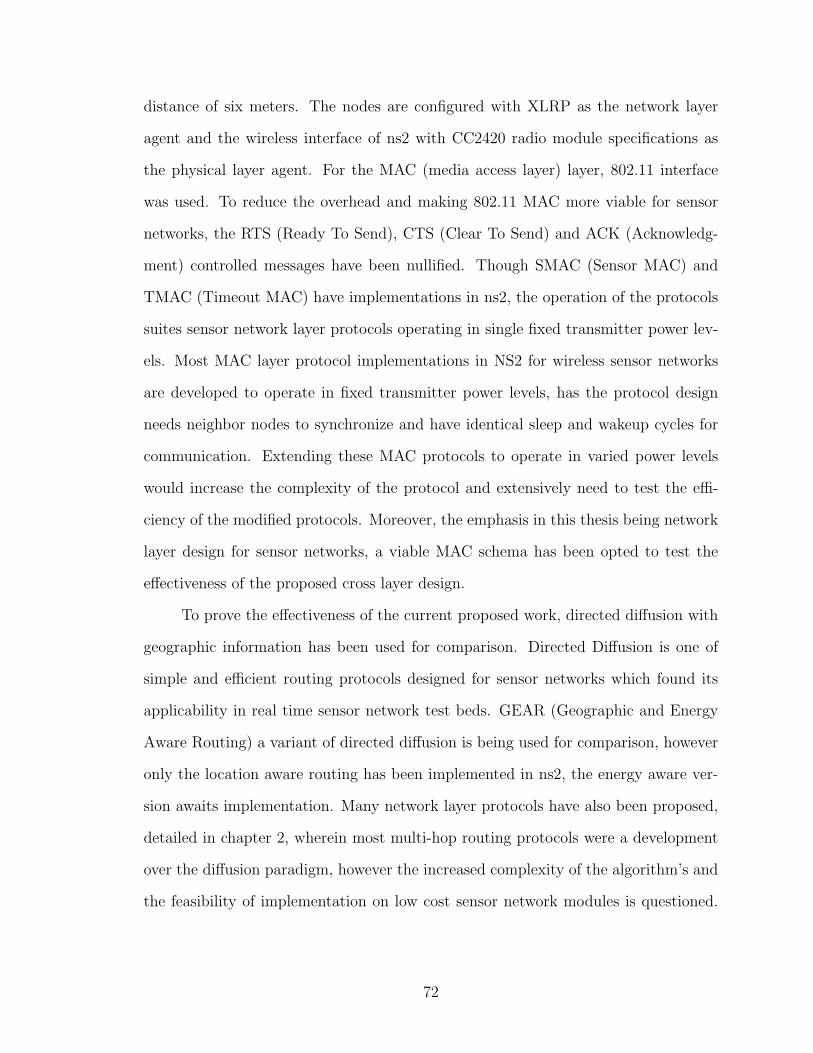
distance of six meters. The nodes are configured with XLRP as the network layer
agent and the wireless interface of ns2 with CC2420 radio module specifications as
the physical layer agent. For the MAC (media access layer) layer, 802.11 interface
was used. To reduce the overhead and making 802.11 MAC more viable for sensor
networks, the RTS (Ready To Send), CTS (Clear To Send) and ACK (Acknowledg-
ment) controlled messages have been nullified. Though SMAC (Sensor MAC) and
TMAC (Timeout MAC) have implementations in ns2, the operation of the protocols
suites sensor network layer protocols operating in single fixed transmitter power lev-
els. Most MAC layer protocol implementations in NS2 for wireless sensor networks
are developed to operate in fixed transmitter power levels, has the protocol design
needs neighbor nodes to synchronize and have identical sleep and wakeup cycles for
communication. Extending these MAC protocols to operate in varied power levels
would increase the complexity of the protocol and extensively need to test the effi-
ciency of the modified protocols. Moreover, the emphasis in this thesis being network
layer design for sensor networks, a viable MAC schema has been opted to test the
effectiveness of the proposed cross layer design.
To prove the effectiveness of the current proposed work, directed diffusion with
geographic information has been used for comparison. Directed Diffusion is one of
simple and efficient routing protocols designed for sensor networks which found its
applicability in real time sensor network test beds. GEAR (Geographic and Energy
Aware Routing) a variant of directed diffusion is being used for comparison, however
only the location aware routing has been implemented in ns2, the energy aware ver-
sion awaits implementation. Many network layer protocols have also been proposed,
detailed in chapter 2, wherein most multi-hop routing protocols were a development
over the diffusion paradigm, however the increased complexity of the algorithm’s and
the feasibility of implementation on low cost sensor network modules is questioned.
72
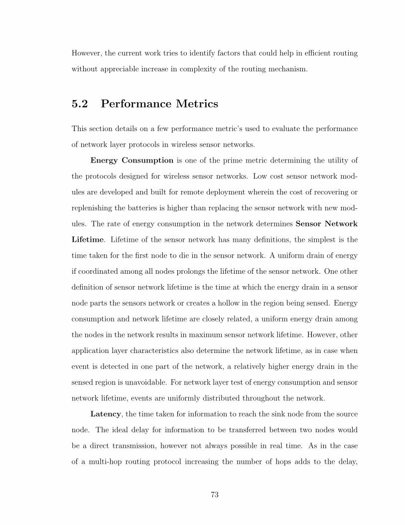
However, the current work tries to identify factors that could help in efficient routing
without appreciable increase in complexity of the routing mechanism.
5.2 Performance Metrics
This section details on a few performance metric’s used to evaluate the performance
of network layer protocols in wireless sensor networks.
Energy Consumption is one of the prime metric determining the utility of
the protocols designed for wireless sensor networks. Low cost sensor network mod-
ules are developed and built for remote deployment wherein the cost of recovering or
replenishing the batteries is higher than replacing the sensor network with new mod-
ules. The rate of energy consumption in the network determines Sensor Network
Lifetime. Lifetime of the sensor network has many definitions, the simplest is the
time taken for the first node to die in the sensor network. A uniform drain of energy
if coordinated among all nodes prolongs the lifetime of the sensor network. One other
definition of sensor network lifetime is the time at which the energy drain in a sensor
node parts the sensors network or creates a hollow in the region being sensed. Energy
consumption and network lifetime are closely related, a uniform energy drain among
the nodes in the network results in maximum sensor network lifetime. However, other
application layer characteristics also determine the network lifetime, as in case when
event is detected in one part of the network, a relatively higher energy drain in the
sensed region is unavoidable. For network layer test of energy consumption and sensor
network lifetime, events are uniformly distributed throughout the network.
Latency, the time taken for information to reach the sink node from the source
node. The ideal delay for information to be transferred between two nodes would
be a direct transmission, however not always possible in real time. As in the case
of a multi-hop routing protocol increasing the number of hops adds to the delay,
73

nevertheless switching to higher power levels would help reduce the number of hops
resulting in faster delivery of information at the node. However, all these performance
parameters are related, for a speedy reception of data energy consumed might be
higher, a tradeoff between energy consumption and latency.
Throughput, a ratio of the number of packets received to that of the packets
transmitted at the network. At the MAC, throughput is an important performance
measure on the MAC layers channel arbitration capability in avoiding data loss due
to collision. However, at the network layer it is based on the successful receipt of
information by intended receivers irrespective of the number of retransmission. In
general TCP/IP based networks throughout is high because of the acknowledgment
message exchanged between nodes, requiring retransmission of packets if not received
correctly. However, in wireless sensor network this would account to huge amount
of information exchange and a source of energy drain in the network. In general in
sensor networks messages are not addressed to nodes rather messages are identified
by their content and forwarded. For example, a data message from source to sink,
the message would be forwarded based on the nodes subscription information.
5.3 Simulation Results
Based on the simulation model elaborated in section 5.1, the effectiveness of the
proposed cross layer routing protocol is being evaluated in reference to the above
discussed performance metrics.
5.3.1 Energy Efficiency
To test the energy efficiency of the protocol a sensor network of 50 nodes was created,
bearing the assumption that nodes are placed such that they have at least one neigh-
bor node that can be reached through its minimum transmitter power level. The
74

0 32 64 128 256 384 5120
5
10
15
20
25
30
35
Data (Packet Size in bytes)
Ene
rgy
(Jou
les)
XLRPGEAR
Figure 5.1: Energy consumption with varying data size
data size was varied and the energy consumed for data transmission between nodes
farther apart, requiring a multi-hop communication, was calculated. Identical net-
work topology was used for comparing XLRP and GEAR. The results of simulation
are shown in fig 5.1. For small packet sizes of 32 or 48 bytes, the energy consumed
was identical for both the protocols, however for increasing packet size XLRP proved
to be consume lesser power compared to that of geographic aware routing. The en-
ergy saving is attributed to the reduction in number of transmitters and controlled
switching OFF of receivers. The high standard deviation in energy for packet sizes
around 256 bytes is because of the higher influence of the communication cost factor
in the decision making process of switching to higher transmitter power levels.
XLRP also had the benefit of switching between neighbor nodes at different
transmitter power along the subscription path, thereby supporting uniform energy
drain along the path. Meaning, though a single path is reinforced with data all
the nodes along the path are not active as nodes alternate radio state by switching
75

transmitter power levels. However, in the case of diffusion based algorithms the energy
drain would be higher for nodes along the path, since in sensor network protocols the
cost of maintaining multiple paths is high.
5.3.2 Reduced Latency
In real time systems, the timely delivery of information is as important as the data
itself. Delay’s beyond a certain bound might no longer be useful at the user end. The
plot in figure 5.2 compares the delay in information being delivered across the network
from a source node to a sink node, the simulation setup is identical to that discussed in
the previous subsection for energy calculations. It is evident from the plot that XLRP
has fifty percent lesser delay compared to that of the directed diffusion paradigm for
the maximum packet size is 512 bytes, this is because of the reduced number of hops
along the transmission path. 512 bytes is set as the maximum physical unit that
can be communicated over the radio by zigbee consortium, detailed in chapter 2.
However, for smaller packet sizes the delay in both the protocols are the same as it is
preferred to remain in lower power transmission mode’s for lower energy consumption.
5.3.3 Scalability
Wireless sensor networked are deemed to operate in large numbers deployed in no
particular fashion. Protocols need to be efficient and prove to be independent of the
network size. Scalability of the protocol has been addressed in terms of increasing
network size with no change in the density of the nodes and increase in node density
by increasing the number of nodes within a region. Scalability of the protocol has
been addressed in terms of the network lifetime, also can be addressed in terms of
the throughput of the sensor network as discussed in the subsequent subsection.
XLRP and GEAR do not have a huge difference in terms of the network life-
time, however XLRP outperforms GEAR. GEAR has high extended network life time
76

0 32 64 128 256 384 5120
50
100
150
200
250
Data(packet size in bytes)
Tra
nsm
issi
on ti
me
(sec
onds
)
XLRPGEAR
Figure 5.2: Latency Measure with respect to data size
77

50 100 150 200 250 300 3500.3
0.4
0.5
0.6
0.7
0.8
0.9
1
Number of Nodes
Nor
mal
ized
Net
wor
k Li
fetim
e
XLRPGEODD (no GEO)
Figure 5.3: Lifetime of the sensor network with increasing network size
because of the knowledge of the location information, as seen in the plot in fig 5.3
compared to that of directed diffusion paradigm with no location information. The
presence of geographic information has the benefits of controlled flooding thereby
saving on energy. However, XLRP outperforms GEAR because of the lesser control
information for the operation of the protocol, GEAR has periodic beacon message
exchange between neighbor node, XLRP does not support any periodic beacons as
in GEAR. However, similar functionalities are achieved by piggy backing information
and gathering information from packets received even though not destined to the
node. Moreover, controlled forwarding is used only for communicating sink messages,
thereby not very beneficial for unicast data messages. In the sensor network lifetime
plots, y axis is labeled normalized network lifetime, calculated as a ratio of energy
exhausted to the total energy available at the instant when the first node is exhausted
of its energy resource.
78

50 75 100 125 1500.3
0.4
0.5
0.6
0.7
0.8
0.9
1
Node Density (Number of Node)
Nor
mal
ized
Net
wor
k Li
fetim
e
XLRPGEAR
Figure 5.4: Lifetime of the sensor network with increasing network density
Also the network lifetime is evaluated with respect to varying node density.
As in fig 5.4, along the x axis the number of nodes increase within a fixed region
thereby increasing on the node density. XLRP shows better performance compared
to that geographic based routing technique, though location information is available,
the information would not be of great help within a specific closed region. XLRP’s
effectiveness is greatly due to the receiver switching characteristic, as a larger number
of unintended receiver nodes can turned OFF. Moreover reduced number of trans-
mission adds to the external network life time of XLRP.
5.3.4 Throughput
Throughput determines the number of packets lost in transmission and that never
reached the intended receiver. Throughput analysis is not confined to data messages,
node identity messages and subscription messages are being accounted for throughput
analysis. Transmission at larger power levels implies larger number of nodes contend
79

50 75 100 125 1500.4
0.5
0.6
0.7
0.8
0.9
1
Node Density (Number of Nodes)
Thr
ough
put
XLRPGEAR
Figure 5.5: Throughput of the network with increasing node density
to send resulting in larger transmissions, however in the present case only unicast
messages are broadcasted at higher power levels, this reduces the number of nodes that
might want to retransmit. Moreover, our concern is in evaluating the performance of
the network layer protocol where in the collision while transmission are not accounted
for, as they are dependent on the MAC layer. In the present case, the reception of
the message is only accounted irrespective of the number of hops or path the message
would take to reach the destination node.
From the plot shown in fig 5.5 with increasing node density the throughput for
the sensor network drops, however gear has a greater slope for drop in throughput
compared to that of XLRP. This is again due to the fact that number of control
message exchange in GEAR is higher compared to that of XLRP where no periodic
control message exchange takes place.
80

Chapter 6
Conclusion and Future Work
This thesis was aimed at identifying and proposing a cross layer routing strategy
for wireless sensors networks, which has been proven efficient in comparison with
that of directed diffusion paradigm in the previous chapter. The concept of using
data size as a feature for routing is uniquely applicable to content aware networked
systems, as in the case of wireless sensor networks deployed for specific applications.
Switching transmitter power levels and dropping packets based on the received signal
strength proves to be an energy efficient and a delay tolerant method for information
dissemination in wireless sensor networks. To conclude with, this chapter details on
the applications and future developments to the proposed work.
6.0.5 Applications
The proposed algorithms finds it’s application in wireless sensor network systems
wherein messages of varied size needs to be exchanged among nodes. Also, for net-
worked sensing systems wherein the volume of information exchange is high and data
needs to be exchanged with specific nodes. Typical application would involve a het-
erogenous sensor network system, wherein the nodes have a wide range of sensing
capabilities and generate data varying from a few bytes to a few hundred kilobytes.
81

For example, a temperature sensor would generate a byte or two bytes of information,
an acoustic sensor would generate a few tens of bytes of data and an image sensor
would generate few hundred bytes of information. Sensor networks being application
specific, built to sense a certain event, one has prior knowledge on what information
would be available from the sensor network. This unique characteristic of sensor net-
work supports size of the data has an unique parameter for routing information and
its unique applicability to sensor networks.
Plans are underway to implement the proposed routing algorithm in a geophone
based wireless sensor network system. Telosb motes are being used as the wireless
sensor network module integrated to a geophone. The network consists of a group
of twenty four or forty eight geophones arranged in an linear fashion, with a master
telosb node attached to a high end computing system like a laptop. The master
node helps logging information generated from the geophones and synchronizing the
geophones for data acquisition. The sensor modules are triggered by an external
source generating seismic signals and the data is acquired by the sensor modules for
a few seconds, 2 to 5 seconds. The motes have a built in ADC (Analog to Digital
Converter) with a resolution of 12 bits, however not built to acquire data has the
negative reference pins for the ADC have been grounded. An external ADC is being
built to acquire the entire peak-to-peak seismic signal and is interfaced to the telosb
motes via serial programmable interface (SPI). Moreover, the application requires
higher data resolution thereby ADS1211 from Texas Instruments is being used as
external ADC which has a maximum bit resolution of 24 bits. With a resolution of
24 bytes and sampling rate in hundreds of microseconds, the data collected would
be around a few hundred kilobytes. This effectively tests the protocol to switch to
higher transmitter power levels for reduced delay and as energy efficient strategy for
data acquisition.
82

The geophone sensor network finds its applicability in structural health moni-
toring, oil explorations, mapping geological features in the earth’s crust, to name a
few. The current setup is a wired network wherein all geophones are spatially sepa-
rated and are wired to a data acquisition box capable of acquiring 48 channels of data
simultaneously. Changing the current setup into an wireless sensing system saves on
time for setting the network and reduces the cost in comparison to the current wired
setup.
6.0.6 Future Work
Having suggested and analyzed the cross layer protocol in detail, possible grounds for
improved performance of the protocol have been identified and are as listed below.
• Node Failures, the advantage of transmission of periodic beacon messages
helps nodes figure out neighbor node loss, however at the expense of energy.
The proposed XLRP algorithm helps acknowledge node loss as a result of en-
ergy exhaustion, however loss due to node malfunction is not accounted for.
This affects the network functionality and data is lost only when messages are
unicast messages. To overcome the problem active nodes on receiving unin-
tended unicast messages of their one hop neighbor nodes, wait for the intended
receiver node to react within a time limit, else the message is locally broadcasted
by the neighbor nodes. Though initially multiple copies of the same message
would be generated as the messages is being forwarded to the source, redundant
messages are further not broadcasted.
• Support for Mobility, the radio signal strength parameter has been widely
used for localization in mobile systems, with the received signal strength pa-
rameter being used in the proposed work, its applicability can be extended to
support mobility in network modules. In the proposed work nodes are identified
83

based on the transmitter power level used for communication. In the case of a
mobile node, which can send out a identity message at periodic intervals and
based on the information received nodes can suitably make changes to their
routing table.
• Include Location Information, the proposed protocol was found to have an
extended network lifetime in comparison with that of location aware diffusion
paradigm. Adding location information to proposed cross layer design would
enhance the network lifetime by limiting interest flooded to geographic regions.
However, this would require specific hardware on the motes to identify them-
selves on the network in a global scale. Nevertheless, using simple radio based
technique to localize node information serves as a low cost alternative but would
increase the complexity of the protocol.
84

Bibliography
85
Bibliography
[1] NS-Manual http://www.isi.edu/nsnam/ns/ns-documentation.html.
[2] D. P. Agrawal A. Manjeshwar. Teen: A routing protocol for enhanced effciency in
wireless sensor networks,. In International Workshop on Parallel and Distributed
Computing Issues in Wireless Networks and Mobile Computing in Conjunction
with the International Parallel and Distributed Processing Symposium (IPDPS),
2001.
[3] K. Akkaya and M. Younis. An energy-aware qos routing protocol for wireless
sensor networks. In Proceedings of the IEEE Workshop on Mobile and Wireless
Networks (MWN 2003), 2003.
[4] K. Akkaya and M. Younis. A survey of routing protocols in wireless sensor
networks. Elsevier Ad Hoc Network Journal, 3(3):329–349, 2005.
[5] Vuran M.C. Akyildiz, I.F. and O.B. Akan. A cross-layer protocol for wireless
sensor networks. In Conference on Information Science and Systems (CISS ’06),
March 22-24 2006.
[6] J.N. Al-Karaki and A.E. Kamal. Routing techniques in wireless sensor networks:
a survey. IEEE Wireless Communications, 11(6):6–28, 2004.
86

[7] David Braginsky and Deborah Estrin. Proceedings of the 1st acm international
workshop on wireless sensor networks and applications. In Rumor routing algo-
rthim for sensor networks, 2002.
[8] J. Chang and L. Tassiulas. Maximum lifetime routing in wireless sensor networks.
IEEE/ACM Transactions on Networking, 12, August 2004.
[9] Kwang-Ting Chuang Cheng-Fu Chou. Colanet: a cross-layer design of energy-
efficient wireless sensor networks. In Proceedings of the Systems Communications,
2005.
[10] P. K. Varshney D. Chen. Qos support in wireless sensor networks: A survey. In
International Conference on Wireless Networks (ICWN), 2004.
[11] John Heidemann Deborah Estrin, Ramesh Govindan and Satish Kumar. Next
century challenges: Scalable coordination in sensor networks. In Proceedings of
the Fifth Annual International Conference on Mobile Computing and Networks
(MobiCOM), August 1999.
[12] T. Voigt H. Ritter J. Schiller Dunkels, J. Alonso. Connecting wireless sensornets
with tcp/ip networks. In Second International Conference on Wired/Wireless
Internet Communications (WWIC2004), February 2004.
[13] S. Lu F. Ye, A. Chen and L. Zhang. A scalable solution to minimum cost
forwarding in large sensor networks. In IEEE International Conference on Com-
puter Communications and Networks, 2001.
[14] Ramesh Govindan Fabio Silva, John Heidemann and Deborah Estrin. Data
gathering in sensor networks using the energy*delay metric. January 2004.
[15] K. Fall. A delay-tolerant network architecture for challenged internets. In SIG-
COMM, 2003.
87
[16] R. Han H. Dai. Unifying micro sensor networks with the internet via overlay
networking. In IEEE Emnets, November 2004.
[17] Jing Wang Ivan Howitt. Energy efficient power control policies for the low rate
wpan. In IEEE Sensor and Ad Hoc Communications and Networks (SECON),
2004.
[18] V. Ailawadhi K. Sohrabi, J. Gao and G. J. Pottie. Protocols for self-organization
of a wireless sensor network. IEEE Personal Communications, 7(5):16–27, 2000.
[19] Koustuv Dasgupta Konstantinos Kalpakis and Parag Namjoshi. Maximum life-
time data gathering and aggregation in wireless sensor networks. In Proceedings
of IEEE Networks Conference, 2002.
[20] Joanna Kulik, Wendi Rabiner Heinzelman, and Hari Balakrishnan. Negotiation-
based protocols for disseminating information in wireless sensor networks. Wire-
less Networks, 8(2-3):169–185, 2002.
[21] Yogesh Sankarasubramaniam Erdal Cayirci lan F. Akyildiz, WellJan Su. A sur-
vey on sensor networks. IEEE Communication Magazine, 40(8):102–114, August
2002.
[22] S. Lindsey and C. S. Raghavendra. Pegasis: Power efficient gathering in sensor
information systems. In IEEE Aerospace Conference, March 2002.
[23] Jian Wu Paul Havinga Lodewijk van Hoesel, Tim Nieberg. Prolonging the life-
time of wireless sensor networks by cross-layer interaction. IEEE Wireless Com-
munication Magazine, 11, December 2004.
[24] A. Manjeshwar and D. P. Agrawal. Apteen: A hybrid protocol for efficient
routing and comprehensive information retrieval in wireless sensor networks. In
88

Proceedings of the 2nd Int. Workshop on Parallel and Distributed Computing
Issues in Wireless Networks and Mobile Computing, 2002.
[25] Horst Haussecker Maurice Chu and Feng Zhao. calable information-driven sensor
querying and routing for ad hoc heterogeneous sensor networks. International
Journal of High Performance Computing Applications, 2002.
[26] Moustafa Youssef Mohamed Younis and Khaled Arisha. Energy-aware routing in
cluster-based sensor networks. In International Symposium on Modeling, Anaysis
and Simulationof Computer and Telecommunication Systems, 2002.
[27] B. Krishnamachari N. Sadagopan and A. Helmy. The acquire mechanism for
efficient querying in sensor networks. In First IEEE International Workshop on
Sensor Network Protocols and Applications (SNPA’03), 2003.
[28] Ahmad Bahai Primoz Skraba, Hamid K. Aghajan. Cross-layer optimization for
high density sensor networks: Distributed passive routing decisions. In Ad-Hoc,
Mobile, and Wireless Networks: Third International Conference, ADHOC-NOW,
2004.
[29] C. Raghavendra S. Lindsey and K. Sivalingam. Data gathering in sensor networks
using the energy*delay metric. IEEE Transactions on Parallel and Distributive
Systems, special issue on Mobile Computing, April 2002.
[30] P.C. Karlsson S. Shakkottai, T.S. Rappaport. Cross-layer design for wireless
networks. IEEE Wireless Communication Magazine, 41:74–80, October 2003.
[31] C. Schurgers and M.B.Srivastava. Energy efficient routing in wireless sensor
networks. In MILCOM Proceedings on Communications for Network-Centric
Operations: Creating the Information Force, 2001.
89

[32] R.C. Shah and J.M. Rabaey. Energy aware routing for low energy ad
hoc sensor networks. In Wireless Communications and Networking Confer-
ence(WCNC2002), March 2002.
[33] L. Subramanian and R. H.Katz. An architecture for building selfconfigurable
systems. In IEEE/ACM Workshop on Mobile Ad Hoc Networking and Computing
(MobiHOC 2000), 2000.
[34] C. Lu T. He, J. Stankovic and T. Abdelzaher. Speed: A stateless protocol
for real-time communication in sensor networks. In 23rd IEEE International
Conference on Distributed Computing Systems (ICDCS’03), 2003.
[35] J. Kulik W. Heinzelman and H. Balakrishnan. Adaptive protocols for information
dissemination in wireless sensor networks. In Proceedings of the Fifth Annual
ACM/IEEE conference on Mobile Computing and Networking (MOBICOM’99),
August 1999.
[36] A. Chandrakasan W. R. Heinzelman and H. Balakrishnan. Energy-efficient com-
munication protocol for wireless microsensor networks. In Proc. of the 33rd
Annual Hawaii International Conference on System Sciences(HICSS), 2000.
[37] R. Govindan Y. Yu and D. Estrin. Geographical and energy aware routing:
a recursive data dissemination protocol for wireless sensor networks. In UCLA
Computer Science Department Technical Report UCLA/CSD-TR-01-0023, 2001.
[38] John Heidemann Ya Xu and Deborah Estrin. Geography-informed energy con-
servation for ad hoc routing. In Proceedings of the Seventh Annual ACM/IEEE
International Conference on Mobile Computing and Networking, 2001.
[39] Y. Yao and J. Gehrke. The cougar approach to in-network query processing in
sensor networks. In SIGMOD Record, Sep 2002.
90

Vita
Raghul Gunasekaran was born in Chennai, India on March 11th 1983. He completed
his high school education at Chinmaya Vidhyalaya, Chennai in the year 2000. Grad-
uated with a bachelor degree in Electronics and Communication Engineering from
the University of Madras in the year 2004. In the spring of 2005 started his Masters
at the Department of Electrical and Computer Engineering, University of Tennessee,
Knoxville. During his graduate studies he joined the Advanced Imaging and Informa-
tion Processing Laboratory of Dr. Hairong Qi majoring in wireless sensor networks.
Associated with the lab, worked on the network layer for wireless sensor networks. He
also held positions as a teaching assistant in the department of Electrical and Com-
puter Engineering during the 2006-07 academic year. During the summer of 2006,
he joined the SensorNet group at Oak Ridge National Laboratory as a graduate stu-
dent intern. He will be graduating with a Master of Science Degree in Electrical
Engineering in May 2007.
91


