Submitted to Journal Geophysical Research, Jan 6, 2004.

A Cumulant-Based Analysis of Nonlinear

Magnetospheric Dynamics

Jay R. Johnson

Princeton University, Plasma Physics Laboratory, Princeton, NJ

Simon Wing

Johns Hopkins University, Applied Physics Laboratory, Laurel, MD

Abstract. Understanding magnetospheric dynamics and predicting futurebehavior of the magnetosphere is of great practical interest because it couldpotentially help to avert catastrophic loss of power and communications. Inorder to build good predictive models it is necessary to understand the mostcritical nonlinear dependencies among observed plasma and electromagneticfield variables in the coupled solar wind/magnetosphere system. In this work,we apply a cumulant-based information dynamical measure to characterizethe nonlinear dynamics underlying the time evolution of the Dst and Kp

geomagnetic indices, given solar wind magnetic field and plasma input. Weexamine the underlying dynamics of the system, the temporal statisticaldependencies, the degree of nonlinearity, and the rate of information loss. Wefind a significant solar cycle dependence in the underlying dynamics of thesystem with greater nonlinearity for solar minimum. The cumulant-basedapproach also has the advantage that it is reliable even in the case of smalldata sets and therefore it is possible to avoid the assumption of stationarity,which allows for a measure of predictability even when the underlyingsystem dynamics may change character. Evaluations of several leading Kp

prediction models indicate that their performances are sub-optimal duringactive times. We discuss possible improvements of these models based on thisnonparametric approach.

1. Introduction

The problem of greatest practical importance inthe area of space physics is that of understandingmagnetospheric response to solar wind input. Thisresponse is expected to be highly nonlinear becausemagnetic energy is stored in the magnetotail and thensuddenly released during violent events termed sub-storms. During these violent releases of energy, en-ergetic MeV electrons, which can damage satelliteinstrumentation, are injected into the ring currentregion. Power service and communications on theground can also be interrupted due to induced cur-rents generated during these massive events. It is

therefore extremely important to be able to predictthe magnetospheric response to solar wind input inorder to be able to make provision for the protectionof scientific, communication and defense satellite in-strumentation as well as ground based power grids.

The most commonly used measure of magneto-spheric activity are the geomagnetic indices obtainedby statistically averaging magnetometer readings fromground-based stations located at various latitudes.The magnetic indices include the planetary index, Kp;the storm index, Dst; and the substorm indices AU,AL, AE, and AO. It is of great interest to under-stand and predict the behavior of these geomagnetic

1

JOHNSON & WING: A Cumulant-Based Analysis ... 2

indices. Because currents induced in power grids andkiller electrons are commonly associated with inten-sification of the ring current associated with storms,they are also associated with the sharp dip in the Dst

index which occurs at the onset of the storm. Ac-curate predictions of the Kp and Dst can be used asinput for the Magnetospheric Specification and Fore-cast Models (MSFM) [Freeman et al., 1995] to pre-dict magnetospheric particle fluxes and electromag-netic fields in the ionosphere. Accurate knowledge ofenergetic particle fluxes and ionospheric fields couldthen be used to provide alerts so that precautionarymeasures could be taken to avoid catastrophic dam-age to power grids and satellites.

Satellites sitting between the sun and earth, e.g.Geotail, WIND, can be used to monitor the input so-lar wind parameters (density, velocity, magnetic fieldstrength and orientation, etc.). The recently launchedACE satellite, which is located at the L1 Lagrangianpoint, has been dedicated to provide solar wind pa-rameters approximately up to one hour before theirarrival, allowing for short term forecasts of the magne-tospheric activity based on these parameters. There-fore, there is a high demand for models that can pre-dict geomagnetic activity accurately based on solarwind parameters as input, a demand that will likelyto increase even more with the nation’s increasing re-liance on the space technologies. Predictability in thiscontext means: given (a) a time series of solar windparameters measured by a satellite sitting in the solarwind and (b) a time series of magnetic index measure-ments, can (A) the value of the geomagnetic index bepredicted accurately at a future time and (B) if so,how far ahead can it be predicted?

Although progress has been made in recent years,comprehensive evaluations of the leading Kp and Dst

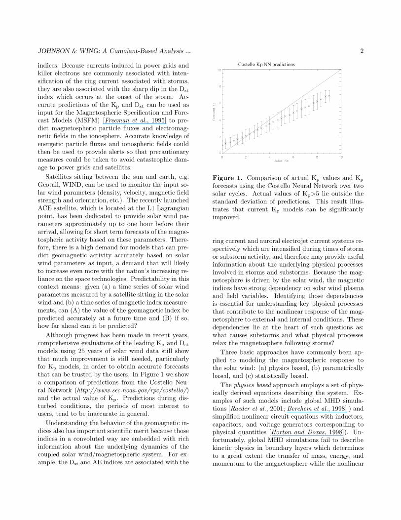
models using 25 years of solar wind data still showthat much improvement is still needed, particularlyfor Kp models, in order to obtain accurate forecaststhat can be trusted by the users. In Figure 1 we showa comparison of predictions from the Costello Neu-ral Network (http://www.sec.noaa.gov/rpc/costello/)and the actual value of Kp. Predictions during dis-turbed conditions, the periods of most interest tousers, tend to be inaccurate in general.

Understanding the behavior of the geomagnetic in-dices also has important scientific merit because thoseindices in a convoluted way are embedded with richinformation about the underlying dynamics of thecoupled solar wind/magnetospheric system. For ex-ample, the Dst and AE indices are associated with the

Costello Kp NN predictions

Figure 1. Comparison of actual Kp values and Kp

forecasts using the Costello Neural Network over twosolar cycles. Actual values of Kp>5 lie outside thestandard deviation of predictions. This result illus-trates that current Kp models can be significantlyimproved.

ring current and auroral electrojet current systems re-spectively which are intensified during times of stormor substorm activity, and therefore may provide usefulinformation about the underlying physical processesinvolved in storms and substorms. Because the mag-netosphere is driven by the solar wind, the magneticindices have strong dependency on solar wind plasmaand field variables. Identifying those dependenciesis essential for understanding key physical processesthat contribute to the nonlinear response of the mag-netosphere to external and internal conditions. Thesedependencies lie at the heart of such questions as:what causes substorms and what physical processesrelax the magnetosphere following storms?

Three basic approaches have commonly been ap-plied to modeling the magnetospheric response tothe solar wind: (a) physics based, (b) parametricallybased, and (c) statistically based.

The physics based approach employs a set of phys-ically derived equations describing the system. Ex-amples of such models include global MHD simula-tions [Raeder et al., 2001; Berchem et al., 1998] ) andsimplified nonlinear circuit equations with inductors,capacitors, and voltage generators corresponding tophysical quantities [Horton and Doxas, 1998]). Un-fortunately, global MHD simulations fail to describekinetic physics in boundary layers which determinesto a great extent the transfer of mass, energy, andmomentum to the magnetosphere while the nonlinear

JOHNSON & WING: A Cumulant-Based Analysis ... 3

circuit models oversimplify the physics.Parametric models assume the response of the

magnetosphere based on expected physical processes(such as particle injection due to solar wind/magnetosphereinteraction and ring current decay due to charge ex-change) which are modeled with parameters that arechosen to minimize the variance between the mea-surements and model predictions. Empirical fore-casting models have been developed—some with amodest number of parameters [e.g. Burton et al.,1975; O’Brien and McPherron, 2000] and others witha more extensive list of parameters [e.g. Li et al.,2001; Temerin and Li, 2002]. This approach usuallyyields plausible results during times of low magne-tospheric activity. Neural network models also pro-vide predictability by assuming an n-step Markovianprocess which can be modeled based on past history.The last n steps are mapped with a parametric nonlin-ear function and then added with parametric weights.The parameters are trained on historical data [Klimaset al., 1997, 1998; Vassiliadis et al., 1995, 1999]. Themodels can then be used to predict system behavior.

Statistical modeling of time series is generally ap-plied to nonlinear time series to understand the un-derlying statistical dependences of the data and toguide in developing an algorithm for accurate predic-tion. Progress has been made in magnetospheric sys-tems by examining the dimensionality of the systemand various correlation measures [Vassiliadis et al.,1990, 1991; Roberts et al., 1991; Sharma, 1995]. Theinformation-theoretic work developed by Prichard et al.[1996] which demonstrated the predictability of thesubstorm dynamics is an innovative approach thathas been widely recognized for its impact on informa-tion technology research and has been widely citedin recent work in the area of information-dynamics.More recent work has focused on the substorm as be-ing a “phase transition” and its possible connectionwith the concept of “self-organized criticality” [Sit-nov et al., 2000; Chang, 1999; Klimas et al., 2000;Lui et al., 2000; Chapman and Watkins, 2001; Changet al., 2003]. However, to date the statistical approachhas not been used as the basis of a predictive model.

While physics based models are well suited to de-scribe and predict long term behavior of a systemfrom physical principles, often the physics is too com-plex to be described accurately by such models. Forexample, some view that the ballooning instabilityis responsible for the onset of substorms which area global phenomena [Roux et al., 1991; Cheng andLui, 1998]. Has this instability ever been identified

in a global MHD simulation? If there were sufficientresolution, would it be possible to describe why mea-surements of the plasma β [Lui et al., 1992] rise wellabove the threshold of the ballooning instability us-ing the global MHD framework? Such issues could beimportant for threshold (onset/timing) of substormsand the dynamical evolution of AE.

Empirical models tend to describe those dynam-ics prescribed to be important by the author ofthe model. Often they involve an extensive num-ber of parameters—many of which may not really bethat important. If the system does not have highdimensionality—and it is believed that the earth’smagnetosphere exhibits low dimensionality [Robertset al., 1991; Sharma, 1995; Vassiliadis et al., 1990]—then it should not require such an extensive number ofparameters. Extensive lists of parameters also makesit difficult to extract the most important underlyingphysics.

Statistical models presume no a priori underlyingdynamics and are therefore useful to flush out the crit-ical nonlinear dependencies in the system. Moreover,the information gained from such an analysis can beinvaluable for developing and constraining parametricmodels.

2. An Information Dynamical Approach

Most data gathered by satellites and ground basedinstruments are in the form of a time series. Ana-lyzing these signals usually encompasses three funda-mental tasks: characterization, forecasting, and mod-eling. Characterization involves determining whatkind of system produced the signal. Forecasting in-volves predicting what the system will do next givenits current state or past history. Modeling involvesdetermining a set of governing equations which de-scribe the evolution of the system [Gershenfeld, 1998].

For complex systems, modeling can be physicallyor computationally difficult. For some systems suchas the brain, physical equations describing neural in-teractions are not well specified. For other systems,such as the magnetosphere, the underlying physicalequations may be known at the most fundamentallevel (particle simulation), but global computationsare beyond present and/or future computational ca-pabilities without appropriate approximations. Em-pirical models that employ intuition assume a prioria dynamical framework that may or may not applyto the system. However, there is some danger in thatit may be possible to fit the data by choosing enough

JOHNSON & WING: A Cumulant-Based Analysis ... 4

free parameters at the expense of loosing physical un-derstanding. Because the magnetospheric system iscomplex and the nonlinear response of the magne-tosphere during storms and substorms is not clearlyunderstood, it seems appropriate to apply statisticaltechniques that are unbiased a priori.

The key to characterizing a system is to under-stand the dependencies in a system. For example,given data from the solar wind and a ground basedmagnetometer, is it possible to determine the degreeto which the magnetometer data depends on the solarwind data? The typical method of choice for discov-ering such dependencies is the correlation function.However, in a highly nonlinear system, correlationfunctions are not very useful because nonlinear sys-tems tend to have broadband power spectra and hencefeatureless correlation structure.

It is well known that the magnetosphere respondsin a highly nonlinear way to solar wind input. Sub-storms involve loading and sudden release of energywhich cannot be well described as a linear system.Therefore, it is necessary to go beyond typical correla-tion studies to understand the nonlinear dependenciesbetween the solar wind driver and the magnetosphericresponse.

Information-theoretic quantities provide an elegantalternative that captures the essential features of thecorrelation function and more [Gershenfeld, 1998].One commonly used information-theoretic quantityis mutual information which provides a statisticalmeasure of dependency based on probability theory[Prichard et al., 1996; Gershenfeld, 1998]. Althoughuseful, it has basic limitations because of the need tocompute a probability density which in many cases re-quires a large database to achieve good statistics. Thecumulant-based significance and information flow arealternative information-theoretic quantities that canbe used to detect dependencies in a system [Deco andSchurmann, 2000]. These quantities provide a mea-sure of the cumulants that would normally vanish inthe absence of dependencies. The significance and in-formation flow are computed directly from the datasetin comparison with surrogate data sets. These mea-sures have an advantage of providing good statisticsfor small data sets and reliable detection of depen-dencies when data is corrupted by noise. In §3 wedefine the cumulant-based information measures andprovide examples of their utility. In §4 we apply thesemeasures to geomagnetic indices and solar wind datato detect the presence of nonlinearities in the solarwind/magnetosphere system.

3. Cumulant-based measure of signifi-cance and information flow

3.1. System Dynamics

The Cumulant-based significance is a useful quan-tify for detecting nonlinearities in the underlying dy-namics of a system. For purposes of explaining ourapproach, let us assume that the underlying dynamicsof a system are described by the evolution of a statevariable x

dxdt

= F(x) + ν (1)

where ν is additive noise. The system dynamics arelinear if

F(x) = a · x (2)

and nonlinear if F is not a linear function of x.In a real system, often only a subset of the state

variables, y, may be observed. Given a limited dataset, it is often useful to consider an embedding vectorof the system

c(t) = {y(t), y(t − 1), ...,y(t− (m − 1)}= {y1, y2, ...,ym}; (3)

The rationale for examining an embedding vector isthat the dynamics of the original system can be cap-tured in the dynamical evolution of the embeddingvector [Takens, 1980; Sauer et al., 1991]. The appli-cation of this concept to the magnetosphere shouldbe obvious. State vectors are generally not knownfor the system as plasma and field measurements arenot available for the entire system as a function oftime (usually only a few single point measurementsare available). These few variables are often com-bined into a single variable that is nonlinearly relatedto appropriate state variables. However, the time evo-lution of that single variable amazingly may containmuch information about the dynamical evolution ofthe entire system.

3.2. Cost and Significance

To detect nonlinearities and understand the un-derlying dynamics of a system, we will examine real-izations of an embedding vector extracted from theoriginal data set (for example, the time history ofDst). We are interested in understanding the pre-dictability of the system, so it is useful to under-stand the probability of finding system in a partic-ular state given past history of the system. For pur-poses of illustration, we construct an embedding vec-

JOHNSON & WING: A Cumulant-Based Analysis ... 5

tor (y1, ..., ym) ≡ (yt, yt−τ , ..., yt−(m−1)τ) from a sin-gle variable, y, in the system. A measure of the rel-evance to the past history on a current/future valueof the system is captured addressed by the followingequation

P (y1, ..., ym) ?=P (y1)P (y2, ..., ym) (4)

where P are probabilities. Equation 4 asks whetherthe probability of extracting the embedding vectory = (y1, ..., ym) depends on the past history (y2, ..., ym).If Equation 4 were true, then there will be certain sta-tistical relations between the higher-order correlationtensors

Ci...j =∫

dyP (y)yi...yj ≡ 〈yi...yj〉 (5)

where i, ..., j ∈ 1, ..., m. In particular, the cumulants,K1i2...in , of the distribution defined by

Ki = Ci = 〈yi〉 (6)Kij = Cij − CiCj = 〈yiyj〉 − 〈yi〉〈yj〉Kijk = Cijk − CijCk − CjkCi − CikCj + 2CiCjCk

Kijkl = Cijkl − CijkCl − CijlCk − CilkCj − CljkCi

−CijCkl − CilCkj − CikCjl + 2(CijCkCl

+CikCjCl + CilCjCk + CjkCiCl + CjlCiCk

+CklCiCj) − 6CiCjCkCl

should vanish unless i2 = ... = in = 1 where n is theorder of the cumulant. Therefore a useful measurethe statistical independence of the components of y1

on (y2, ..., yn), is the cost function defined as:

D =∞∑

n=1

m∑i2,...,in=1

(1 − δ1i2...in){K1i2...in}2 (7)

where δij...n is the Kronecker delta which eliminatesthe diagonal elements. In the absence of correla-tions, the cost function should vanish. To examinethe significance of correlations, we employ the methodof surrogates. The method consists of assuming anull hypothesis, constructing surrogate data consis-tent with that hypothesis, and then comparing thecost function for the original data set with the costfunctions of the surrogate data sets. The significanceis defined as:

S =|D0 − µS |

σS(8)

where D0 is the cost of the original data set µS andσS are the mean and variance of the costs computedwith the surrogate data sets,

µs =1N

N∑i=1

DSi (9)

σS =1

N − 1

N∑i=1

(DSi − µS)2. (10)

where N is the number of surrogate data sets.The surrogate data is chosen consistent with a null

hypothesis which for our purposes will be that thereis no causal relationship between the past and thepresent. The surrogate data may be obtained by tak-ing random permutations of the original data set orby extracting data randomly from the same densitydistribution as the original dataset. If the signifi-cance is larger than S = 1.67, there is a 95% chancethat the null hypothesis is falsified and that there is aclear underlying dynamics governing the system (notethat erfc(S/2) = 0.05) assuming Gaussianity in thesurrogates distribution which is typically true if thenumber of surrogates is sufficiently large) [Deco andSchurmann, 2000]. If the significance remains roughlyconstant, the dynamics are stationary, but if the sig-nificance changes in magnitude during time, it sug-gests that the dynamics involved are non-stationary.The technique was tested on a number of datasetsgenerated by mathematical equations for which theunderlying dynamics is known prior to application tothe magnetospheric datasets.

The significance can be useful for a number of tasks[Deco and Schurmann, 2000]:

• By comparing the significance when keepingonly second-order cumulants with the signifi-cance including higher-order cumulants, we maydetermine whether the origin of the observedstatistical correlations are linear or nonlinear.The second order cumulant is equivalent to thecorrelation function.

• As in a spectrogram, we can also consider win-dowed significance where data is sampled from awindow of width Nw and a significance is com-puted for that data set. The window is thenshifted and the significance recomputed. Timevariations in the significance indicate changes inthe underlying dynamics of the system.

• We can introduce a proxy for the informationflow based on cumulant-based significance in-tegrated over ”look ahead.” Information flowdeals with changes in the information contentof a system. The information flow can be usedto detect changes in underlying dynamics andthe loss of information in a system. The loss of

JOHNSON & WING: A Cumulant-Based Analysis ... 6

information in a system can be quantified andprovides a measure of the predictability horizonof the system. Such calculations are practicalbecause if there is a characteristic time for in-formation loss in a system, it would be foolishto attempt to develop parametric models to pre-dict system behavior on longer time scales.

3.3. Significance as a Measure of Nonlinearity

By comparing the significance when keeping onlysecond-order cumulants with the significance includ-ing higher-order cumulants, we may also determinewhether the origin of the observed statistical corre-lations are linear or nonlinear. We Gaussianize thedata set in order to eliminate the effect of ”static”nonlinearities in the original data set [Kennel and Is-abelle, 1992] as described in § 3.5. Statistical studiesare then performed on the Gaussianized data whichexhibits no static nonlinearity (all cumulants vanishbeyond second order).

We present two example which illustrate the utilityof the method. The first example is the well-knownLorenz system [Lorenz, 1963] which satisfies the fol-lowing equations:

dx

dt= σ(y − x)

dy

dt= −xz + rx − y

dz

dt= xy − bz (11)

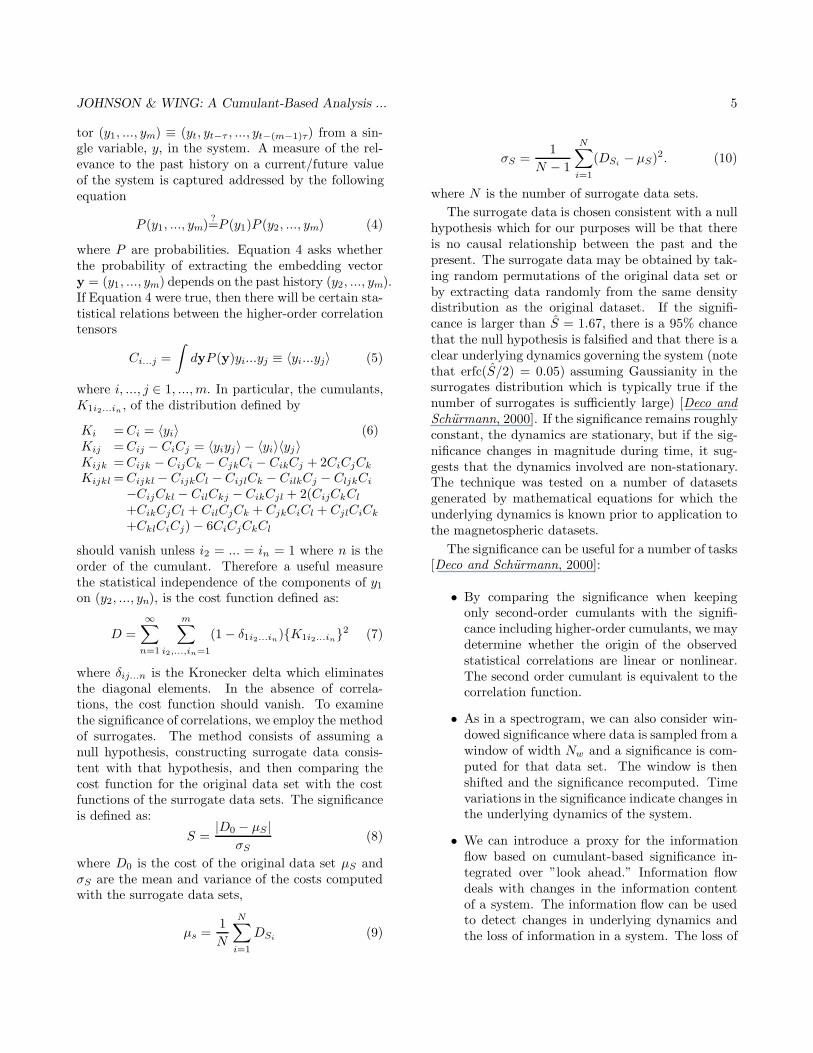
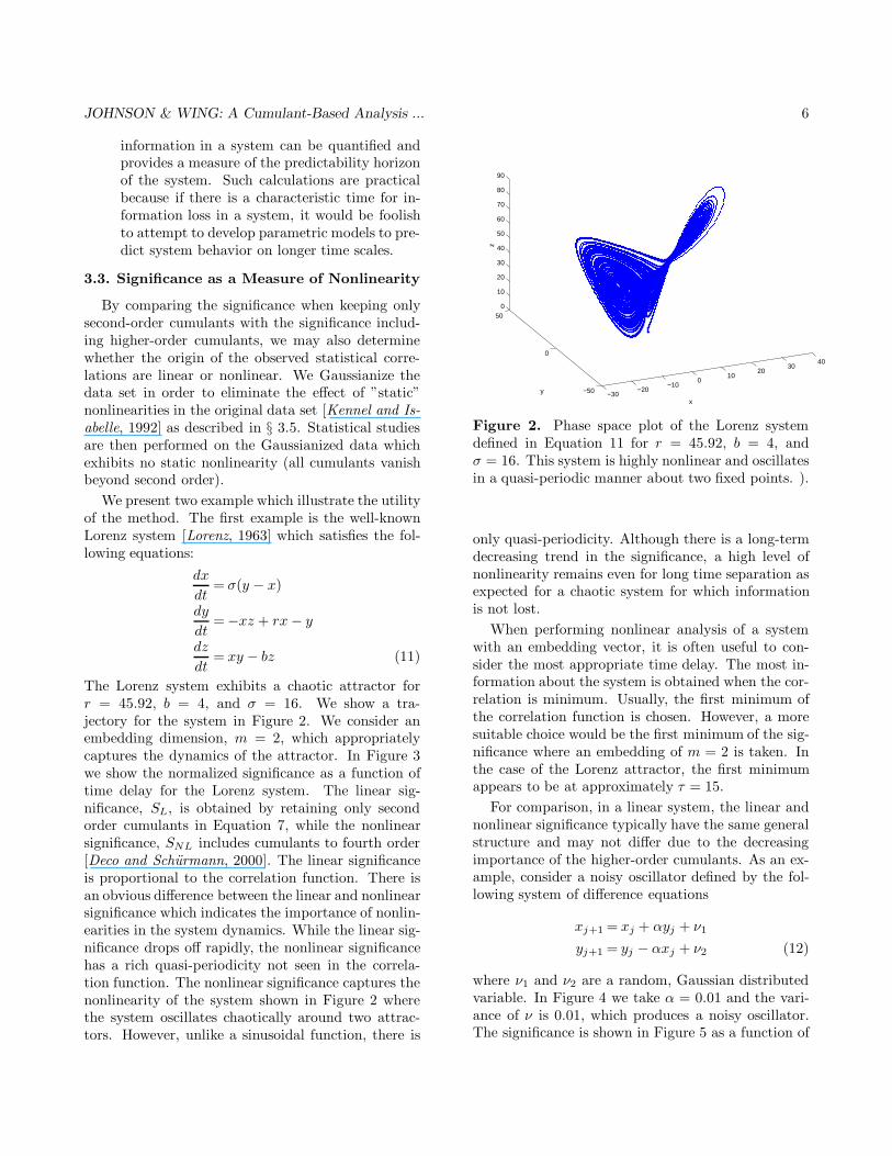
The Lorenz system exhibits a chaotic attractor forr = 45.92, b = 4, and σ = 16. We show a tra-jectory for the system in Figure 2. We consider anembedding dimension, m = 2, which appropriatelycaptures the dynamics of the attractor. In Figure 3we show the normalized significance as a function oftime delay for the Lorenz system. The linear sig-nificance, SL, is obtained by retaining only secondorder cumulants in Equation 7, while the nonlinearsignificance, SNL includes cumulants to fourth order[Deco and Schurmann, 2000]. The linear significanceis proportional to the correlation function. There isan obvious difference between the linear and nonlinearsignificance which indicates the importance of nonlin-earities in the system dynamics. While the linear sig-nificance drops off rapidly, the nonlinear significancehas a rich quasi-periodicity not seen in the correla-tion function. The nonlinear significance captures thenonlinearity of the system shown in Figure 2 wherethe system oscillates chaotically around two attrac-tors. However, unlike a sinusoidal function, there is

−30−20

−100

1020

3040

−50

0

500

10

20

30

40

50

60

70

80

90

x

y

z

Figure 2. Phase space plot of the Lorenz systemdefined in Equation 11 for r = 45.92, b = 4, andσ = 16. This system is highly nonlinear and oscillatesin a quasi-periodic manner about two fixed points. ).

only quasi-periodicity. Although there is a long-termdecreasing trend in the significance, a high level ofnonlinearity remains even for long time separation asexpected for a chaotic system for which informationis not lost.

When performing nonlinear analysis of a systemwith an embedding vector, it is often useful to con-sider the most appropriate time delay. The most in-formation about the system is obtained when the cor-relation is minimum. Usually, the first minimum ofthe correlation function is chosen. However, a moresuitable choice would be the first minimum of the sig-nificance where an embedding of m = 2 is taken. Inthe case of the Lorenz attractor, the first minimumappears to be at approximately τ = 15.

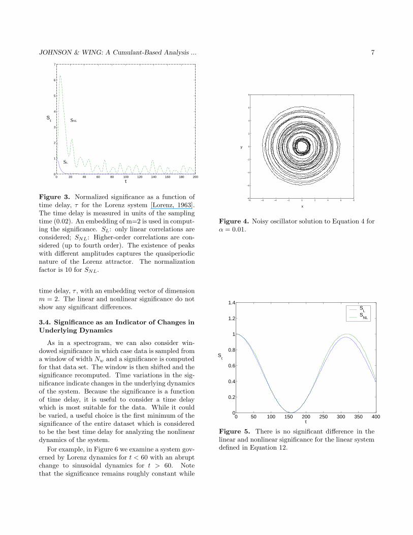
For comparison, in a linear system, the linear andnonlinear significance typically have the same generalstructure and may not differ due to the decreasingimportance of the higher-order cumulants. As an ex-ample, consider a noisy oscillator defined by the fol-lowing system of difference equations

xj+1 = xj + αyj + ν1

yj+1 = yj − αxj + ν2 (12)

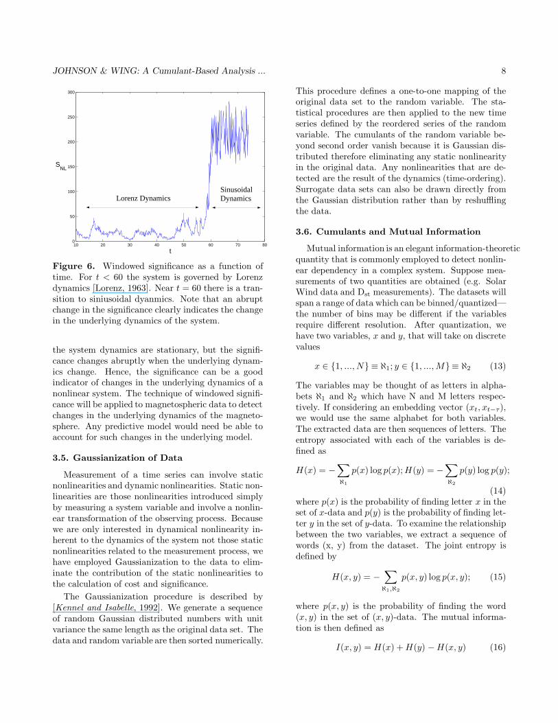
where ν1 and ν2 are a random, Gaussian distributedvariable. In Figure 4 we take α = 0.01 and the vari-ance of ν is 0.01, which produces a noisy oscillator.The significance is shown in Figure 5 as a function of

JOHNSON & WING: A Cumulant-Based Analysis ... 7

0 20 40 60 80 100 120 140 160 180 2000

1

2

3

4

5

6

7

τ

Sτ SNL

SL

Figure 3. Normalized significance as a function oftime delay, τ for the Lorenz system [Lorenz, 1963].The time delay is measured in units of the samplingtime (0.02). An embedding of m=2 is used in comput-ing the significance. SL: only linear correlations areconsidered; SNL: Higher-order correlations are con-sidered (up to fourth order). The existence of peakswith different amplitudes captures the quasiperiodicnature of the Lorenz attractor. The normalizationfactor is 10 for SNL.

time delay, τ , with an embedding vector of dimensionm = 2. The linear and nonlinear significance do notshow any significant differences.

3.4. Significance as an Indicator of Changes inUnderlying Dynamics

As in a spectrogram, we can also consider win-dowed significance in which case data is sampled froma window of width Nw and a significance is computedfor that data set. The window is then shifted and thesignificance recomputed. Time variations in the sig-nificance indicate changes in the underlying dynamicsof the system. Because the significance is a functionof time delay, it is useful to consider a time delaywhich is most suitable for the data. While it couldbe varied, a useful choice is the first minimum of thesignificance of the entire dataset which is consideredto be the best time delay for analyzing the nonlineardynamics of the system.

For example, in Figure 6 we examine a system gov-erned by Lorenz dynamics for t < 60 with an abruptchange to sinusoidal dynamics for t > 60. Notethat the significance remains roughly constant while

−8 −6 −4 −2 0 2 4 6 8−8

−6

−4

−2

0

2

4

6

8

x

y

Figure 4. Noisy oscillator solution to Equation 4 forα = 0.01.

0 50 100 150 200 250 300 350 4000

0.2

0.4

0.6

0.8

1

1.2

1.4

Sτ

τ

SL

SNL

Figure 5. There is no significant difference in thelinear and nonlinear significance for the linear systemdefined in Equation 12.

JOHNSON & WING: A Cumulant-Based Analysis ... 8

10 20 30 40 50 60 70 800

50

100

150

200

250

300

t

SNL

Lorenz DynamicsSinusoidalDynamics

Figure 6. Windowed significance as a function oftime. For t < 60 the system is governed by Lorenzdynamics [Lorenz, 1963]. Near t = 60 there is a tran-sition to siniusoidal dyanmics. Note that an abruptchange in the significance clearly indicates the changein the underlying dynamics of the system.

the system dynamics are stationary, but the signifi-cance changes abruptly when the underlying dynam-ics change. Hence, the significance can be a goodindicator of changes in the underlying dynamics of anonlinear system. The technique of windowed signifi-cance will be applied to magnetospheric data to detectchanges in the underlying dynamics of the magneto-sphere. Any predictive model would need be able toaccount for such changes in the underlying model.

3.5. Gaussianization of Data

Measurement of a time series can involve staticnonlinearities and dynamic nonlinearities. Static non-linearities are those nonlinearities introduced simplyby measuring a system variable and involve a nonlin-ear transformation of the observing process. Becausewe are only interested in dynamical nonlinearity in-herent to the dynamics of the system not those staticnonlinearities related to the measurement process, wehave employed Gaussianization to the data to elim-inate the contribution of the static nonlinearities tothe calculation of cost and significance.

The Gaussianization procedure is described by[Kennel and Isabelle, 1992]. We generate a sequenceof random Gaussian distributed numbers with unitvariance the same length as the original data set. Thedata and random variable are then sorted numerically.

This procedure defines a one-to-one mapping of theoriginal data set to the random variable. The sta-tistical procedures are then applied to the new timeseries defined by the reordered series of the randomvariable. The cumulants of the random variable be-yond second order vanish because it is Gaussian dis-tributed therefore eliminating any static nonlinearityin the original data. Any nonlinearities that are de-tected are the result of the dynamics (time-ordering).Surrogate data sets can also be drawn directly fromthe Gaussian distribution rather than by reshufflingthe data.

3.6. Cumulants and Mutual Information

Mutual information is an elegant information-theoreticquantity that is commonly employed to detect nonlin-ear dependency in a complex system. Suppose mea-surements of two quantities are obtained (e.g. SolarWind data and Dst measurements). The datasets willspan a range of data which can be binned/quantized—the number of bins may be different if the variablesrequire different resolution. After quantization, wehave two variables, x and y, that will take on discretevalues

x ∈ {1, ..., N} ≡ ℵ1; y ∈ {1, ..., M} ≡ ℵ2 (13)

The variables may be thought of as letters in alpha-bets ℵ1 and ℵ2 which have N and M letters respec-tively. If considering an embedding vector (xt, xt−τ),we would use the same alphabet for both variables.The extracted data are then sequences of letters. Theentropy associated with each of the variables is de-fined as

H(x) = −∑ℵ1

p(x) log p(x); H(y) = −∑ℵ2

p(y) log p(y);

(14)where p(x) is the probability of finding letter x in theset of x-data and p(y) is the probability of finding let-ter y in the set of y-data. To examine the relationshipbetween the two variables, we extract a sequence ofwords (x, y) from the dataset. The joint entropy isdefined by

H(x, y) = −∑ℵ1,ℵ2

p(x, y) log p(x, y); (15)

where p(x, y) is the probability of finding the word(x, y) in the set of (x, y)-data. The mutual informa-tion is then defined as

I(x, y) = H(x) + H(y) − H(x, y) (16)

JOHNSON & WING: A Cumulant-Based Analysis ... 9

0 10 20 30 40 50 60 70 80 90 1000

0.2

0.4

0.6

0.8

1

1.2

1.4

1.6

1.8

2

τ

I(xt,x

t − τ)

0 10 20 30 40 50 60 70 80 90 1000

10

20

30

40

50

60

τ

Sτ

a)

b)

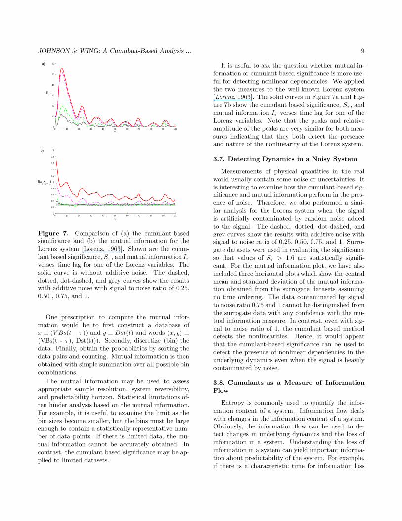
Figure 7. Comparison of (a) the cumulant-basedsignificance and (b) the mutual information for theLorenz system [Lorenz, 1963]. Shown are the cumu-lant based significance, Sτ , and mutual information Iτ

verses time lag for one of the Lorenz variables. Thesolid curve is without additive noise. The dashed,dotted, dot-dashed, and grey curves show the resultswith additive noise with signal to noise ratio of 0.25,0.50 , 0.75, and 1.

One prescription to compute the mutual infor-mation would be to first construct a database ofx ≡ (V Bs(t − τ )) and y ≡ Dst(t) and words (x, y) ≡(VBs(t - τ ), Dst(t))). Secondly, discretize (bin) thedata. Finally, obtain the probabilities by sorting thedata pairs and counting. Mutual information is thenobtained with simple summation over all possible bincombinations.

The mutual information may be used to assessappropriate sample resolution, system reversibility,and predictability horizon. Statistical limitations of-ten hinder analysis based on the mutual information.For example, it is useful to examine the limit as thebin sizes become smaller, but the bins must be largeenough to contain a statistically representative num-ber of data points. If there is limited data, the mu-tual information cannot be accurately obtained. Incontrast, the cumulant based significance may be ap-plied to limited datasets.

It is useful to ask the question whether mutual in-formation or cumulant based significance is more use-ful for detecting nonlinear dependencies. We appliedthe two measures to the well-known Lorenz system[Lorenz, 1963]. The solid curves in Figure 7a and Fig-ure 7b show the cumulant based significance, Sτ , andmutual information Iτ verses time lag for one of theLorenz variables. Note that the peaks and relativeamplitude of the peaks are very similar for both mea-sures indicating that they both detect the presenceand nature of the nonlinearity of the Lorenz system.

3.7. Detecting Dynamics in a Noisy System

Measurements of physical quantities in the realworld usually contain some noise or uncertainties. Itis interesting to examine how the cumulant-based sig-nificance and mutual information perform in the pres-ence of noise. Therefore, we also performed a simi-lar analysis for the Lorenz system when the signalis artificially contaminated by random noise addedto the signal. The dashed, dotted, dot-dashed, andgrey curves show the results with additive noise withsignal to noise ratio of 0.25, 0.50, 0.75, and 1. Surro-gate datasets were used in evaluating the significanceso that values of Sτ > 1.6 are statistically signifi-cant. For the mutual information plot, we have alsoincluded three horizontal plots which show the centralmean and standard deviation of the mutual informa-tion obtained from the surrogate datasets assumingno time ordering. The data contaminated by signalto noise ratio 0.75 and 1 cannot be distinguished fromthe surrogate data with any confidence with the mu-tual information measure. In contrast, even with sig-nal to noise ratio of 1, the cumulant based methoddetects the nonlinearities. Hence, it would appearthat the cumulant-based significance can be used todetect the presence of nonlinear dependencies in theunderlying dynamics even when the signal is heavilycontaminated by noise.

3.8. Cumulants as a Measure of InformationFlow

Entropy is commonly used to quantify the infor-mation content of a system. Information flow dealswith changes in the information content of a system.Obviously, the information flow can be used to de-tect changes in underlying dynamics and the loss ofinformation in a system. Understanding the loss ofinformation in a system can yield important informa-tion about predictability of the system. For example,if there is a characteristic time for information loss

JOHNSON & WING: A Cumulant-Based Analysis ... 10

in a system, it would be foolish to attempt to de-velop parametric models to predict system behavioron longer time scales.

The flow of information in a system is best definedin terms of a conditional entropy, H, which measuresthe uncertainty of a variable x(t+p) given all possiblepreceding sequences of that variable.

Ip = limn→∞[H(x(t + p)|x(t), ..., x(t− n + 1)

−H(x(t + p − 1)|x(t), ..., x(t− n + 1)] (17)

In the case of a chaotic system, there is no loss ofmemory and information flow is constant. On theother hand, for a noisy system information flow de-creases with increasing look ahead. Development ofpredictive models is not practicable beyond the decaylength of the information flow.

Unfortunately, it is usually difficult to compute astatistically meaningful information flow for a realsystem because of the limited size of the data set.However, cumulants which also carry informationabout the underlying system dynamics are readily ob-tained even from limited data sets. We can thereforeintroduce a proxy for for the information flow whichwe define as the cumulant-based information flow

IC(p) =∞∑

n=1

m∑i2,...,in=1

(1 − δ1i2...in){K(p)1i2...in

}2 (18)

where K(p)1i2...in are the cumulants associated withthe vector {y1, ..., ym} = {y(t + p), y(t − ∆), ..., y(t−(m − 1)∆)}. This quantity provides an estimate ofhow well a predictive model could estimate a futurevalue of the time series p steps ahead given the pasthistory of the time series. The minimal value ofIc(p) = 0 indicates statistical independence while in-creasing values of IC(p) point to increasing dependen-cies in the time series [Deco and Schurmann, 2000].Ideally, m should be chosen large enough so that IC(p)becomes a measure of predictability given the entirepast of the time series. For practical purposes, wechoose the value of m such that the information flowdoes not change appreciably when m is increased. Asfor the case of significance, we limit the computationto the fourth-order cumulant.

While the information flow IC(p) provides an indi-cation of how far into the future one should be ableto predict the time series, when examining changes inthe information flow, it is more practical to consider

0 100 200 300 400 500 600 700 800 900 10000.1

0.2

0.3

0.4

0.5

0.6

0.7

0.8

0.9

1

1.1Information Flow for Lorenz Sequence

IC(p)

p

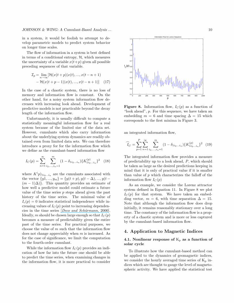
Figure 8. Information flow, IC(p) as a function of“look ahead”, p. For this sequence, we have taken anembedding m = 6 and time spacing ∆ = 15 whichcorresponds to the first minima in Figure 3.

an integrated information flow,

I�

C =P∑

p=1

∞∑n=1

m∑i2,...,in=1

(1 − δ1i2...in){K(p)1i2...in

}2 (19)

The integrated information flow provides a measureof predictability up to a look ahead, P , which shouldbe taken as large as the desired predictions keeping inmind that it is only of practical value if it is smallerthan value of p which characterizes the falloff of theinformation flow IC (p)

As an example, we consider the Lorenz attractorsystem defined in Equation 11. In Figure 8 we plotIC(p) for that system. We have taken an embed-ding vector, m = 6, with time separation ∆ = 15.Note that although the information flow does dropinitially, it remains reasonably stationary over a longtime. The constancy of the information flow is a prop-erty of a chaotic system and is more or less capturedby the cumulant-based information flow.

4. Application to Magnetic Indices

4.1. Nonlinear response of Kp as a function ofsolar cycle

To illustrate how the cumulant-based method canbe applied to the dynamics of geomagnetic indices,we consider the hourly averaged time series of Kp in-dices which are thought to gauge the level of magneto-spheric activity. We have applied the statistical test

JOHNSON & WING: A Cumulant-Based Analysis ... 11

0 50 100 150 2000

0.1

0.2

0.3

0.4

0.5

0.6

0.7

0.8

0.9

1Normalized Significance of Kp data from 1975

Sτ

τ

SL

SNL

0 50 100 150 2000

0.1

0.2

0.3

0.4

0.5

0.6

0.7

0.8

0.9

1Normalized Significance of Kp data from 1987

Sτ

τ

SL

SNL

a)

b)

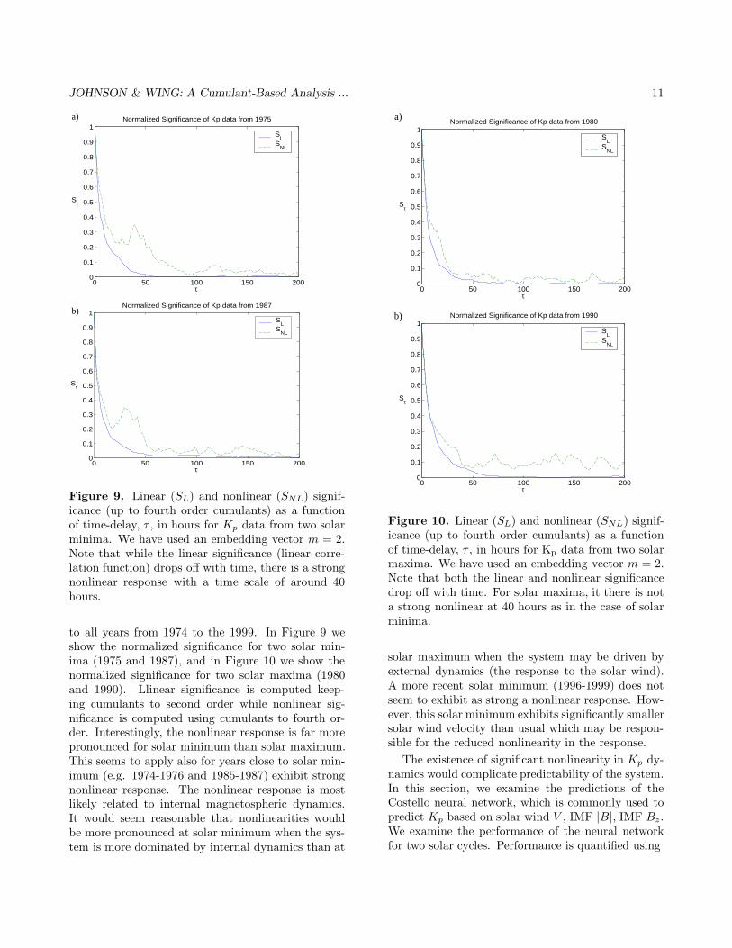
Figure 9. Linear (SL) and nonlinear (SNL) signif-icance (up to fourth order cumulants) as a functionof time-delay, τ , in hours for Kp data from two solarminima. We have used an embedding vector m = 2.Note that while the linear significance (linear corre-lation function) drops off with time, there is a strongnonlinear response with a time scale of around 40hours.

to all years from 1974 to the 1999. In Figure 9 weshow the normalized significance for two solar min-ima (1975 and 1987), and in Figure 10 we show thenormalized significance for two solar maxima (1980and 1990). Llinear significance is computed keep-ing cumulants to second order while nonlinear sig-nificance is computed using cumulants to fourth or-der. Interestingly, the nonlinear response is far morepronounced for solar minimum than solar maximum.This seems to apply also for years close to solar min-imum (e.g. 1974-1976 and 1985-1987) exhibit strongnonlinear response. The nonlinear response is mostlikely related to internal magnetospheric dynamics.It would seem reasonable that nonlinearities wouldbe more pronounced at solar minimum when the sys-tem is more dominated by internal dynamics than at

0 50 100 150 2000

0.1

0.2

0.3

0.4

0.5

0.6

0.7

0.8

0.9

1Normalized Significance of Kp data from 1980

Sτ

τ

SL

SNL

0 50 100 150 2000

0.1

0.2

0.3

0.4

0.5

0.6

0.7

0.8

0.9

1Normalized Significance of Kp data from 1990

Sτ

τ

SL

SNL

a)

b)

Figure 10. Linear (SL) and nonlinear (SNL) signif-icance (up to fourth order cumulants) as a functionof time-delay, τ , in hours for Kp data from two solarmaxima. We have used an embedding vector m = 2.Note that both the linear and nonlinear significancedrop off with time. For solar maxima, it there is nota strong nonlinear at 40 hours as in the case of solarminima.

solar maximum when the system may be driven byexternal dynamics (the response to the solar wind).A more recent solar minimum (1996-1999) does notseem to exhibit as strong a nonlinear response. How-ever, this solar minimum exhibits significantly smallersolar wind velocity than usual which may be respon-sible for the reduced nonlinearity in the response.

The existence of significant nonlinearity in Kp dy-namics would complicate predictability of the system.In this section, we examine the predictions of theCostello neural network, which is commonly used topredict Kp based on solar wind V , IMF |B|, IMF Bz.We examine the performance of the neural networkfor two solar cycles. Performance is quantified using

JOHNSON & WING: A Cumulant-Based Analysis ... 12

Solid Line: TSSDash Line: GS

Kp=2 Kp=3

Kp=4 Kp=5

Kp=6 Solar Max

Solar Max

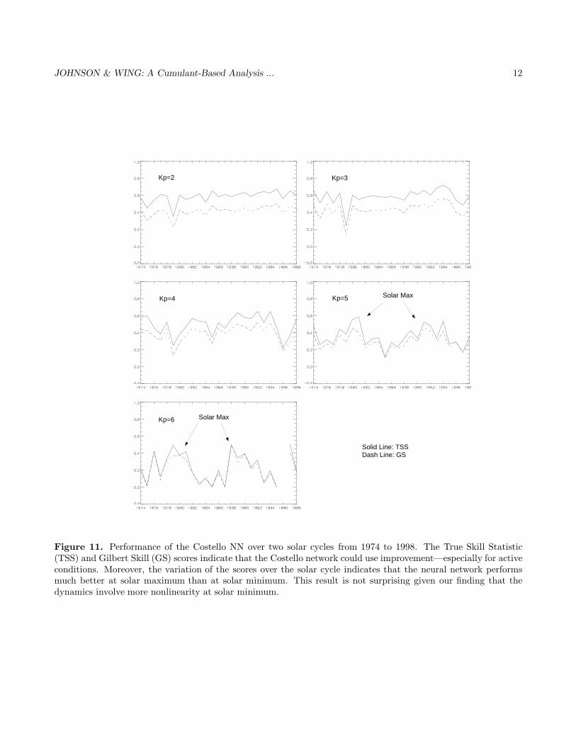
Figure 11. Performance of the Costello NN over two solar cycles from 1974 to 1998. The True Skill Statistic(TSS) and Gilbert Skill (GS) scores indicate that the Costello network could use improvement—especially for activeconditions. Moreover, the variation of the scores over the solar cycle indicates that the neural network performsmuch better at solar maximum than at solar minimum. This result is not surprising given our finding that thedynamics involve more nonlinearity at solar minimum.

JOHNSON & WING: A Cumulant-Based Analysis ... 13

skill scores defined in [Detman and Joselyn, 1999].In Figure 11 we show predictive model performance

as a function of solar cycle for various values of Kp.We plot True Skill Statistics (TSS) and Gilbert Skill(GS) scores for the neural network model. Whilethere is no significant difference in predictive abilityfor Kp < 3, there is a significant solar cycle depen-dence for Kp > 3. In either case, there is significantroom for improvement. It is also clear that there isbetter predictability at solar maximum than at solarminimum. Although this result may be related to atraining bias, it may also reflect the increased nonlin-earity of the system dynamics for solar minimum.

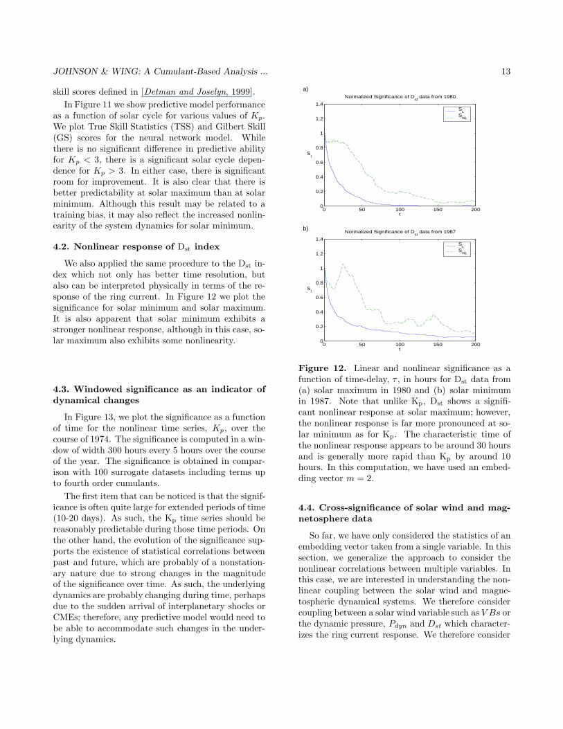
4.2. Nonlinear response of Dst index

We also applied the same procedure to the Dst in-dex which not only has better time resolution, butalso can be interpreted physically in terms of the re-sponse of the ring current. In Figure 12 we plot thesignificance for solar minimum and solar maximum.It is also apparent that solar minimum exhibits astronger nonlinear response, although in this case, so-lar maximum also exhibits some nonlinearity.

4.3. Windowed significance as an indicator ofdynamical changes

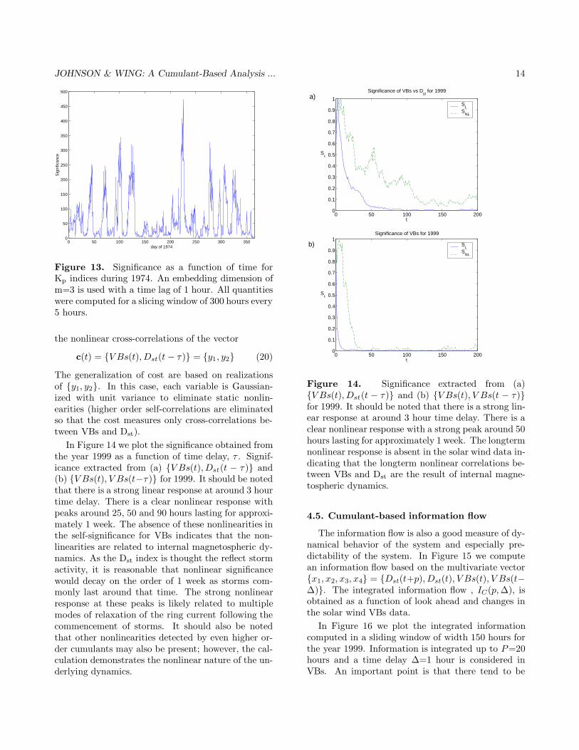
In Figure 13, we plot the significance as a functionof time for the nonlinear time series, Kp, over thecourse of 1974. The significance is computed in a win-dow of width 300 hours every 5 hours over the courseof the year. The significance is obtained in compar-ison with 100 surrogate datasets including terms upto fourth order cumulants.

The first item that can be noticed is that the signif-icance is often quite large for extended periods of time(10-20 days). As such, the Kp time series should bereasonably predictable during those time periods. Onthe other hand, the evolution of the significance sup-ports the existence of statistical correlations betweenpast and future, which are probably of a nonstation-ary nature due to strong changes in the magnitudeof the significance over time. As such, the underlyingdynamics are probably changing during time, perhapsdue to the sudden arrival of interplanetary shocks orCMEs; therefore, any predictive model would need tobe able to accommodate such changes in the under-lying dynamics.

0 50 100 150 2000

0.2

0.4

0.6

0.8

1

1.2

1.4

Normalized Significance of Dst

data from 1980

Sτ

τ

SL

SNL

0 50 100 150 2000

0.2

0.4

0.6

0.8

1

1.2

1.4

Normalized Significance of Dst

data from 1987

Sτ

τ

SL

SNL

a)

b)

Figure 12. Linear and nonlinear significance as afunction of time-delay, τ , in hours for Dst data from(a) solar maximum in 1980 and (b) solar minimumin 1987. Note that unlike Kp, Dst shows a signifi-cant nonlinear response at solar maximum; however,the nonlinear response is far more pronounced at so-lar minimum as for Kp. The characteristic time ofthe nonlinear response appears to be around 30 hoursand is generally more rapid than Kp by around 10hours. In this computation, we have used an embed-ding vector m = 2.

4.4. Cross-significance of solar wind and mag-netosphere data

So far, we have only considered the statistics of anembedding vector taken from a single variable. In thissection, we generalize the approach to consider thenonlinear correlations between multiple variables. Inthis case, we are interested in understanding the non-linear coupling between the solar wind and magne-tospheric dynamical systems. We therefore considercoupling between a solar wind variable such as V Bs orthe dynamic pressure, Pdyn and Dst which character-izes the ring current response. We therefore consider

JOHNSON & WING: A Cumulant-Based Analysis ... 14

0 50 100 150 200 250 300 3500

50

100

150

200

250

300

350

400

450

500

day of 1974

Sig

nific

ance

Figure 13. Significance as a function of time forKp indices during 1974. An embedding dimension ofm=3 is used with a time lag of 1 hour. All quantitieswere computed for a slicing window of 300 hours every5 hours.

the nonlinear cross-correlations of the vector

c(t) = {V Bs(t), Dst(t − τ )} = {y1, y2} (20)

The generalization of cost are based on realizationsof {y1, y2}. In this case, each variable is Gaussian-ized with unit variance to eliminate static nonlin-earities (higher order self-correlations are eliminatedso that the cost measures only cross-correlations be-tween VBs and Dst).

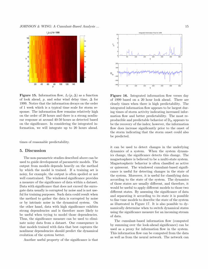
In Figure 14 we plot the significance obtained fromthe year 1999 as a function of time delay, τ . Signif-icance extracted from (a) {V Bs(t), Dst(t − τ )} and(b) {V Bs(t), V Bs(t−τ )} for 1999. It should be notedthat there is a strong linear response at around 3 hourtime delay. There is a clear nonlinear response withpeaks around 25, 50 and 90 hours lasting for approxi-mately 1 week. The absence of these nonlinearities inthe self-significance for VBs indicates that the non-linearities are related to internal magnetospheric dy-namics. As the Dst index is thought the reflect stormactivity, it is reasonable that nonlinear significancewould decay on the order of 1 week as storms com-monly last around that time. The strong nonlinearresponse at these peaks is likely related to multiplemodes of relaxation of the ring current following thecommencement of storms. It should also be notedthat other nonlinearities detected by even higher or-der cumulants may also be present; however, the cal-culation demonstrates the nonlinear nature of the un-derlying dynamics.

0 50 100 150 2000

0.1

0.2

0.3

0.4

0.5

0.6

0.7

0.8

0.9

1

Significance of VBs vs Dst

for 1999

Sτ

τ

SL

SNL

0 50 100 150 2000

0.1

0.2

0.3

0.4

0.5

0.6

0.7

0.8

0.9

1Significance of VBs for 1999

Sτ

τ

SL

SNL

a)

b)

Figure 14. Significance extracted from (a){V Bs(t), Dst(t − τ )} and (b) {V Bs(t), V Bs(t − τ )}for 1999. It should be noted that there is a strong lin-ear response at around 3 hour time delay. There is aclear nonlinear response with a strong peak around 50hours lasting for approximately 1 week. The longtermnonlinear response is absent in the solar wind data in-dicating that the longterm nonlinear correlations be-tween VBs and Dst are the result of internal magne-tospheric dynamics.

4.5. Cumulant-based information flow

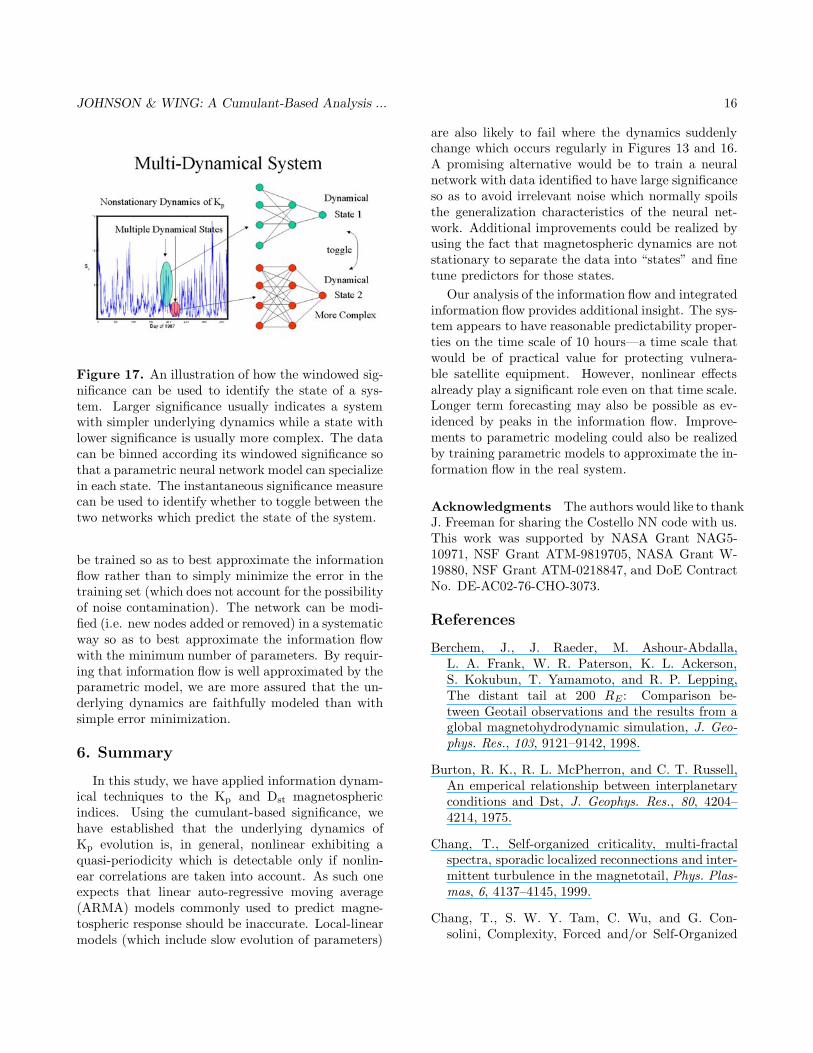
The information flow is also a good measure of dy-namical behavior of the system and especially pre-dictability of the system. In Figure 15 we computean information flow based on the multivariate vector{x1, x2, x3, x4} = {Dst(t+p), Dst(t), V Bs(t), V Bs(t−∆)}. The integrated information flow , IC(p, ∆), isobtained as a function of look ahead and changes inthe solar wind VBs data.

In Figure 16 we plot the integrated informationcomputed in a sliding window of width 150 hours forthe year 1999. Information is integrated up to P=20hours and a time delay ∆=1 hour is considered inVBs. An important point is that there tend to be

JOHNSON & WING: A Cumulant-Based Analysis ... 15

Figure 15. Information flow, IC(p, ∆) as a functionof look ahead, p, and solar wind delay time, ∆ for1999. Notice that the information decays on the orderof 1 week which is a typical time scale for storm re-sponse. The information flow remains relatively highon the order of 20 hours and there is a strong nonlin-ear response at around 40-50 hours as detected basedon the significance. In considering the integrated in-formation, we will integrate up to 20 hours ahead.

times of reasonable predictability.

5. Discussion

The non-parametric studies described above can beused to guide development of parametric models. Theoutput from models depends heavily on the methodby which the model is trained. If a training set isnoisy, for example, the output is often spoiled or notwell constrained. The windowed significance providesa measure of the significance of data within a dataset.Data with significance that does not exceed the surro-gate data usually is corrupted by noise and is not use-ful for training purposes. Such data could result whenthe method to gather the data is corrupted by noiseor by intrinsic noise in the dynamical system. Onthe other hand, data with high significance exhibitsstrong dependencies and is therefore more likely tobe useful when trying to model those dependencies.Thus, the significance measure can be used to elimi-nate noisy data from a dataset. One consequence isthat models trained with data that best captures thenonlinear dependencies should predict the dynamicalevolution of the system better.

Another useful property of the significance is that

0 50 100 150 200 250 300 3500

2

4

6

8

10Integrated Information Flow for 1999

IC

t

0 50 100 150 200 250 300 350−300

−200

−100

0

100

200

Dst

t

Figure 16. Integrated information flow verses dayof 1999 based on a 20 hour look ahead. There areclearly times when there is high predictability. Theintegrated information flow appears to be largest dur-ing times of storm activity indicating increased infor-mation flow and better predictability. The most re-producible and predictable behavior of Dst appears tobe the recovery of the index; however, the informationflow does increase significantly prior to the onset ofthe storm indicating that the storm onset could alsobe predicted.

it can be used to detect changes in the underlyingdynamics of a system. When the system dynam-ics change, the significance detects this change. Themagnetosphere is believed to be a multi-state system.Magnetospheric behavior is often classified as activeor quiescent. The windowed cumulant-based signifi-cance is useful for detecting changes in the state ofthe system. Moreover, it is useful for classifying dataaccording to the state of the system. The dynamicsof those states are usually different, and therefore, itwould be useful to apply different models to those twodifferent states. By assessing the significance of dataand separating it according to its state it is possibleto fine tune models to describe the state of the systemas illustrated in Figure 17. It is also possible to dy-namically determine when to switch dynamical statesusing the significance measure for an incoming streamof data.

The cumulant-based information flow (computedby summing over the look-ahead significance) can beused as a proxy for information flow in the system.This information flow can be computed from the dataas well as from the neural network. The network can

JOHNSON & WING: A Cumulant-Based Analysis ... 16

Figure 17. An illustration of how the windowed sig-nificance can be used to identify the state of a sys-tem. Larger significance usually indicates a systemwith simpler underlying dynamics while a state withlower significance is usually more complex. The datacan be binned according its windowed significance sothat a parametric neural network model can specializein each state. The instantaneous significance measurecan be used to identify whether to toggle between thetwo networks which predict the state of the system.

be trained so as to best approximate the informationflow rather than to simply minimize the error in thetraining set (which does not account for the possibilityof noise contamination). The network can be modi-fied (i.e. new nodes added or removed) in a systematicway so as to best approximate the information flowwith the minimum number of parameters. By requir-ing that information flow is well approximated by theparametric model, we are more assured that the un-derlying dynamics are faithfully modeled than withsimple error minimization.

6. Summary

In this study, we have applied information dynam-ical techniques to the Kp and Dst magnetosphericindices. Using the cumulant-based significance, wehave established that the underlying dynamics ofKp evolution is, in general, nonlinear exhibiting aquasi-periodicity which is detectable only if nonlin-ear correlations are taken into account. As such oneexpects that linear auto-regressive moving average(ARMA) models commonly used to predict magne-tospheric response should be inaccurate. Local-linearmodels (which include slow evolution of parameters)

are also likely to fail where the dynamics suddenlychange which occurs regularly in Figures 13 and 16.A promising alternative would be to train a neuralnetwork with data identified to have large significanceso as to avoid irrelevant noise which normally spoilsthe generalization characteristics of the neural net-work. Additional improvements could be realized byusing the fact that magnetospheric dynamics are notstationary to separate the data into “states” and finetune predictors for those states.

Our analysis of the information flow and integratedinformation flow provides additional insight. The sys-tem appears to have reasonable predictability proper-ties on the time scale of 10 hours—a time scale thatwould be of practical value for protecting vulnera-ble satellite equipment. However, nonlinear effectsalready play a significant role even on that time scale.Longer term forecasting may also be possible as ev-idenced by peaks in the information flow. Improve-ments to parametric modeling could also be realizedby training parametric models to approximate the in-formation flow in the real system.

Acknowledgments The authors would like to thankJ. Freeman for sharing the Costello NN code with us.This work was supported by NASA Grant NAG5-10971, NSF Grant ATM-9819705, NASA Grant W-19880, NSF Grant ATM-0218847, and DoE ContractNo. DE-AC02-76-CHO-3073.

References

Berchem, J., J. Raeder, M. Ashour-Abdalla,L. A. Frank, W. R. Paterson, K. L. Ackerson,S. Kokubun, T. Yamamoto, and R. P. Lepping,The distant tail at 200 RE: Comparison be-tween Geotail observations and the results from aglobal magnetohydrodynamic simulation, J. Geo-phys. Res., 103, 9121–9142, 1998.

Burton, R. K., R. L. McPherron, and C. T. Russell,An emperical relationship between interplanetaryconditions and Dst, J. Geophys. Res., 80, 4204–4214, 1975.

Chang, T., Self-organized criticality, multi-fractalspectra, sporadic localized reconnections and inter-mittent turbulence in the magnetotail, Phys. Plas-mas, 6, 4137–4145, 1999.

Chang, T., S. W. Y. Tam, C. Wu, and G. Con-solini, Complexity, Forced and/or Self-Organized

JOHNSON & WING: A Cumulant-Based Analysis ... 17

Criticality, and Topological Phase Transitions inSpace Plasmas, Space Science Reviews, 107, 425–445, 2003.

Chapman, S., and N. Watkins, Avalanching andSelf-Organised Criticality, a paradigm for geomag-netic activity?, Space Science Reviews, 95, 293–307, 2001.

Cheng, C. Z., and A. T. Y. Lui, Kinetic ballooning in-stability for substorm onset and current disruptionobserved by AMPTE/CCE, Geophys. Res. Lett.,25, 4091–4094, 1998.

Deco, G., and B. Schurmann, Information Dynamics.Springer, 2000.

Detman, T., and J. A. Joselyn, Real-time Kp predic-tions from ACE real time solar wind, in Solar WindNine, edited by S. R. Habbal, R. Esser, J. V. Holl-weg, and P. A. Isenberg, pp. 729–732. The Ameri-can Institute of Physics, 1-56396-865-7, 1999.

Freeman, J. W., et al., The magnetosphericspecification and forecast model, preprintavailable at http://hydra.rice.edu/ free-man/ding/www/msfm95/index.html, 1995.

Gershenfeld, N., The Nature of Mathematical Mod-eling. Cambridge University Press, Cambridge,chapter, 1998.

Horton, W., and I. Doxas, A low-dimensional dy-namical model for the solar wind driven geotail-ionosphere system, J. Geophys. Res., 103, 4561–4572, 1998.

Kennel, M. B., and S. Isabelle, Method to dinstin-guish possible chaos from colored noise and to de-termine embedding parameters, Phys. Rev. A, 46,3111, 1992.

Klimas, A., J. A. Valdivia, D. Vassiliadis, D. N.Baker, M. Hesse, and J. Takalo, Self-organizedcriticality in the substorm phenomenon and itsrelation to localized reconnection in the magne-tospheric plasma sheet, J. Geophys. Res., 105,18,765–18,780, 2000.

Klimas, A. J., D. Vassiliadis, and D. N. Baker, Data-derived analogues of the magnetospheric dynamics,J. Geophys. Res., 102, 26993–27010, 1997.

Klimas, A. J., D. Vassiliadis, and D. N. Baker, Dstindex prediction using data-derived analogues ofthe magnetospheric dynamics, J. Geophys. Res.,103, 20435–20448, 1998.

Li, X., M. Temerin, D. N. Baker, G. D. Reeves, andD. Larson, Quantitative Prediction of RadiationBelt Electrons at Geostationary Orbit Based onSolar Wind Measurements, Geophys. Res. Lett.,28, 1887, 2001.

Lorenz, E., Deterministic nonperiodic flows, J. Atmo-sph. Sci., 96, 5877–5882, 1963.

Lui, A. T. Y., et al., Current disruptions in the near-Earth neutral sheet region, J. Geophys. Res., 97,1461, 1992.

Lui, A. T. Y., S. C. Chapman, K. Liou, P. T. Newell,C. I. Meng, M. Brittnacher, and G. K. Parks, Is thedynamic magnetosphere an avalanching system?,Geophys. Res. Lett., 27, 911, 2000.

O’Brien, T. P., and R. L. McPherron, An empiricalphase space analysis of ring current dynamics: So-lar wind control of injection and decay, J. Geophys.Res., 105, 7707–7720, 2000.

Prichard, D., J. E. Borovsky, P. M. Lemons, andC. P. Price, Time dependence of substorm recur-rence: An information-theoretic analysis, J. Geo-phys. Res., 101, 15359–15370, 1996.

Raeder, J., et al., Global simulation of the GeospaceEnvironment Modeling substorm challenge event,J. Geophys. Res., 106, 381–396, 2001.

Roberts, D. A., D. N. Baker, A. J. Klimas, andL. F. Bargatze, Indications of low dimensionalityin magnetospheric dynamics, Geophys. Res. Lett.,18, 151–154, 1991.

Roux, A., S. Perraut, A. Morane, P. Robert, A. Ko-rth, G. .Kremser, A. Pederson, R. Pellinen, andZ. Y. Pu, Plasma sheet instability related to thewestward traveling surge, J. Geophys. Res., 96,17697, 1991.

Sauer, T., J. Yorke, and M. Casdagli, Embedology,Journal of Statistical Physics, 65, 579, 1991.

Sharma, A. S., Assessing the magnetosphere’s nonlin-ear behavior: Its dimension is low, its predictibil-ity, high, Rev. Geophys., 33, 645–650, 1995.

JOHNSON & WING: A Cumulant-Based Analysis ... 18

Sitnov, M. I., A. S. Sharma, K. Papadopoulos, D. Vas-siliadis, J. A. Valdivia, A. J. Klimas, and D. N.Baker, Phase transition-like behavior of the mag-netosphere during substorms, J. Geophys. Res.,105, 12955–12974, 2000.

Takens, F., Detecting strange attractors in tur-bulence., in Dynamical Systems and Turbulence,edited by D. A. Rand, and L. S. Young, vol. 898of Lecture Notes in Mathematics, p. 366. Springer-Verlag, 1980.

Temerin, M., and X. Li, A new model for the predic-tion of Dst on the basis of the solar wind, Journalof Geophysical Research (Space Physics), pp. 31–1,2002.

Vassiliadis, D., A. S. Sharma, and K. Papadopou-los, Lyapunov exponent of magnetospheric activ-ity from AL time series, Geophys. Res. Lett., 18,1643–1646, 1991.

Vassiliadis, D., A. J. Klimas, D. N. Baker, andD. A. Roberts, A description of the solar wind-magnetosphere coupling based on nonlinear filters,J. Geophys. Res., 100, 3495–3512, 1995.

Vassiliadis, D., A. J. Klimas, J. A. Valdivia, and D. N.Baker, The Dst geomagnetic response as a functionof storm phase and amplitude and the solar windelectric field, J. Geophys. Res., 104, 24957–24976,1999.

Vassiliadis, D. V., A. S. Sharma, T. E. Eastman, andK. Papadopoulos, Low-dimensional chaos in mag-netospheric activity from AE time series, Geophys.Res. Lett., 17, 1841–1844, 1990.

This preprint was prepared with the AGU LATEX macrosv3.0. File CUM formatted 2004 January 28.

With the extension package ‘AGU++’, version 1.2 from1995/01/12