Submitted to the Journal of Guidance, Control, and DynamicsThe Nonlinear Projection FilterRandal Beard� Jacob Gunther Jonathan Lawton Wynn StirlingDepartment of Electrical and Computer EngineeringBrigham Young UniversityProvo, Utah 84602

AbstractThe conditional probability density function of the state of a stochas-tic dynamic system represents the complete solution to the nonlinear�ltering problem because, with the conditional density in hand, all es-timates of the state, optimal or otherwise, can be computed. It is wellknown that, for systems with continuous dynamics, the conditional den-sity evolves, between measurements, according to Kolmogorov's forwardequation. At a measurement, it is updated according to Bayes formula.Therefore, these two equations can be viewed as the dynamic equationsof the conditional density and, hence, the exact nonlinear �lter. In thispaper, Galerkin's method is used to approximate the nonlinear �lter bysolving for the entire conditional density. Using an FFT to approximate�Corresponding Author, email: beard@ee.byu.edu.1

the projections required in Galerkin's method leads to a computation-ally e�cient nonlinear �lter. The implementation details are given andperformance is assessed through simulations.Nomenclature(A)ij The (i; j)th element of the matrix A.FFT[f(�)] The fast Fourier transform of a function f at N uniformsamples between the limits a and b.I The identity matrix.IFFT[f(�)] The inverse fast Fourier transform of a function f at Nuniform samples between the limits a and b.p(t; xjYt) The conditional density of the state of the state of thesystem, given the measurement sequence Yt = fyk : tk �tgpN(t; xjYt) The Galerkin approximation of p(t; xjYt).p̂ The truncation of p(t; xjYt) to the closed and boundedset .p(yk+1jx) e� 12 [yk�h(x;tk)]TR�1k [yk�h(x;tk)]p(2�)mjRkj .p(t�k+1; xjYtk) The solution of the Kolmogorov equation at time t�k+1.<(z) The real part of the complex number z.t�k+1 The instant in time right before the k + 1st sample.f�`g1̀=1 A complete set of basis functions for L2.2

1 IntroductionEstimating the state of a stochastic dynamic system from noisy observationsis an important problem in engineering. The extensive work on this problemfor linear systems was initiated by Kalman and Bucy.1,2 In the decades sincethis early work, many important theoretical results for the linear problem haveemerged and the linear �lter has found wide practical application. However,since most systems are not truly linear, linear �ltering theory does not applydirectly to most physical systems.In the more general setting of nonlinear systems, �lter theory is less devel-oped but has received attention from a number of researchers since the 1960's(c.f.3{6). For linear systems with Gaussian inputs, the probability density func-tion of the state conditioned on the measurements is Gaussian. Hence, optimallinear �lters need only propagate the conditional mean and covariance whichcompletely describes the density function. However, for nonlinear systems, theconditional density may not have a �nite parameterization. General nonlinear�lters must therefore propagate the entire density function.The extended Kalman �lter (EKF), a heuristic �lter based on the linearizeddynamics of a system system,7{10 has become a standard for state estimationof nonlinear systems. The EKF assumes (1) that deviations from the referencestate trajectory are small, (2) that the mathematical description of the systemdynamics and observations is accurate and (3) that the conditional densityfunction of the state is Gaussian. For large deviations from the reference3

trajectory, the extended Kalman �lter performs poorly or becomes unstable.Furthermore, if constructed from an erroneous model, the EKF state estimatescan diverge from the true state. In addition, due to the nonlinear nature ofthe EKF, its estimate may depend on the initial conditions of the �lter. In the�nal section of this paper, we show an example where the EKF gives erroneousresults if it is not correctly initialized.In this paper, we construct a nonlinear �lter which approximates the ex-act nonlinear �lter for systems with continuous nonlinear dynamics and dis-crete nonlinear observations. Accordingly, the paper represents a departurefrom current research directions in nonlinear �ltering. Rather than pursueenhancements or modi�cations of the EKF, or explore dual relationships tovarious non-optimal control algorithms, we investigate a reasonable methodof approximating the exact nonlinear �ltering problem. We note that if theexact nonlinear �ltering problem could be solved directly or approximated ef-�ciently, that it would be widely used today in various industrial applications.We feel that this paper represents a signi�cant step in that direction.The exact nonlinear �lter consists of two dynamic equations:3� A partial di�erential equation (Kolmogorov's forward equation) that de-scribes how the conditional density evolves between measurements and� A di�erence equation (Bayes formula) that describes how it is modi�edby information supplied by new measurements.To solve these equations we employ Galerkin's method, a classic procedure for4

approximating solutions of partial di�erential equations.11,12Galerkin's method assumes that the exact solution to a partial di�erentialequation can be expanded as an in�nite sum of basis elements. An approx-imate solution is found by truncating this sum and projecting the resultingerror onto the �nite subspace spanned by the basis elements used to approx-imate the solution.11 To distinguish the approximate �lter from the exact�lter, and for lack of a better name, we will refer to the resulting �lter as theNonlinear Projection Filter (NPF). Using a complex exponential basis as ap-proximating elements, we show that the nonlinear �lter can be implementede�ciently (for low order systems) using Fast Fourier Transforms (FFT) re-sulting in a fast nonlinear �lter which could be implemented real-time on adigital signal processor. Sinusoidal bases have been used before to implementGalerkin-based algorithms, but in much di�erent contexts.13{15 This work isalso a natural extension of the application of Galerkin's method to optimaland robust control.16{19 To our knowledge, this is the �rst time these ideashave been applied to the nonlinear �ltering problem.An important issue concerns the convergence of the Galerkin approxima-tion. We shall prove that the approximation residual converges to zero as thedimension of the �nite dimensional subspace used in the approximation tendsto in�nity. In other words, the NPF converges to the exact nonlinear �lter.One limitation in our convergence result is that we do not obtain an explicitestimate of the approximation error. We only show that the approximation5

error can be made arbitrarily small by making the order of the approximationlarge enough.Since the NPF is an approximation of the exact nonlinear �lter, it canoutperform the extended Kalman �lter for large variations in the state, formodel mismatches, and for arbitrary initial conditions. In addition, since wepropagate the conditional density, we can compute optimal state estimatesfor any criterion. In contrast, the extended Kalman �lter is only capable ofapproximating the conditional mean.The remainder of the paper is organized as follows. The nonlinear �lter-ing problem and the exact nonlinear �lter is given in Section 2. In Section 3,Galerkin's method is used to approximate the exact nonlinear �lter resulting inthe Nonlinear Projection Filter. In Section 4 we show that the NPF convergesto the exact nonlinear �lter as the order of approximation increases. Practi-cal implementation of the �lter, and the use of exponential basis elements isdiscussed in Section 5. Finally, Section 6 contains simulations comparing theNonlinear Projection Filter and the extended Kalman �lter.2 Exact Nonlinear FilterMost physical systems evolve continuously in time while measurements mayonly be taken periodically at discrete time instants. Suppose the n-dimensional6

state xt of a continuous nonlinear stochastic dynamic system satis�esdxt = f(t; xt)dt+G(t; xt)d�t; t � t0 (1)where f�t; t � t0g is a p-dimensional Brownian motion with covariance matrixQ(t)dt. Let m-dimensional noisy measurements be made at discrete times tkyk = h(xtk ; tk) + vk; k = 1; 2; � � � (2)where fvk; k � 1g is a m-dimensional white Gaussian sequence independent ofd�t with covariance matrix Rk. De�ne the collection of measurements taken upto and including time t as Yt = fyk : tk � tg. We seek equations of evolutionfor the conditional density p(t; xjYt) since it summarizes all the statisticalinformation about the state contained in the measurements Yt and the initialcondition p(t0; x). From p(t; xjYt), the conditional mean and variance can becomputed, which for nonlinear systems, generally depend upon all the higherorder moments.Between observations at tk and tk+1, p � p(t; xjYt) di�uses according toKolmogorov's forward equation@p@t = � nXi=1 @(pfi)@xi + 12 nXi=1 nXj=1 @2[p(GQGT )ij]@xi@xj (3)where either p(t0; x) or p(tk; xjYtk), the measurement update at tk, is used asthe initial condition. At an observation, p satis�es the di�erence equationp(tk+1; xjYtk+1) = p(yk+1jx)p(t�k+1; xjYtk)R p(yk+1j�)p(�; t�k+1jYtk)d� : (4)7

For a detailed derivation and discussion of these results see.3Equations (3) and (4) represent dynamic equations for the exact nonlinear�lter. Equation (3) is used to compute predictions between measurements,while measurements are used to update the information about the state viaEquation (4). There are only a few special cases where this set of equationshas a closed form solution. For example, for a linear dynamic system driven byGaussian noise, this �lter reduces to the standard Kalman �lter.3 In the nextsection we show that Galerkin's approximation method can be used to reduceEquation (3) to a linear ordinary di�erential equation, and Equation (4) to analgebraic update equation.3 Approximate Filter3.1 Prediction EquationIn this section we use the global or spectral Galerkin approximation methodto reduce the Equation (3) from a function of space and time to a function oftime only. The result is a linear ordinary di�erential equation which is easyto solve numerically. Galerkin's method is discussed in most textbooks onpartial di�erential equations. Particularly good introductions to the topic canbe found in.11,12,20To apply Galerkin's method, we �rst assume that the solution of Equa-tion (3) satis�es p(t; xjYt) = P1̀=0 b`(t)�`(x) where equality is in the sense of8

the L2 norm. We approximate p by truncating the sum:pN(t; xjYn) 4= N�1X̀=0 c`(t)�`(x); (5)where the coe�cients c` satisfy the projection equationZ0@@pN@t + nXi=1 @(pNfi)@xi � 12 nXi=1 nXj=1 @2[pN (GQGT )ij]@xi@xj 1A�q dx = 0;for q = 0; : : : ; N � 1. Since p does not have compact support, the set shouldbe Rn . However, p will be almost zero over most of Rn . Practically we mustselect to be a closed and bounded subset of Rn . The convergence resultsin Section 4 assume that is a su�ciently large compact set. Interchangingsummation and di�erentiation we obtainN�1X̀=0 _c` Z �`�q dx = N�1X̀=0 c`8<:� nXi=1 Z @[�`fi]@xi �q dx + 12 nXi=1 nXj=1 Z @2[�`(GQGT )ij]@xi@xj �q dx9=; ;(6)for q = 0; : : : ; N �1. Equation (6) is a system of N linear ordinary di�erentialequations which may be written in matrix notation by de�ningc = [c0; � � � ; cN�1]T ;[M]i;j = Z �i�j dx; (7)[A1(t)]i;j = � nXk=1 Z @[�jfk]@xk �i dx; (8)[A2(t)]i;j = 12 nXk=1 nX̀=1 Z @2[�j(GQGT )k`]@xk@x` �i dx: (9)With these de�nitions, equation (6) can be rewritten asM _c = (A1(t) +A2(t))c:9

Letting AN(t) =M�1(A1(t) +A2(t)) we have_c(t) = AN(t)c(t):The initial condition for this ordinary di�erential equation can be obtainedfrom either the initial density function p(t0; x) or from the measurement updatep(tk; xjYtk). In the next subsection we will show how to obtain the initialcoe�cients in the case of a measurement update. At time t = t0 the initialcoe�cients are obtained by choosing c(t0) such thatZ p(t0; x)�q dx = Z pN(x; t0jYt0)�q dx= N�1X̀=0 c`(t0) Z �`�q dxfor q = 0; � � � ; N � 1. To write this in matrix notation de�nes 4= [Z p(t0; x)�0 dx; � � � ; Z p(t0; x)�N�1 dx]T :The initial conditions then become Mc(t0) = s or c(t0) =M�1s.We have therefore converted Equation (3) describing the evolution of p intoa system of ordinary di�erential equations_cN(t) = AN(t)cN(t); cN(t0) =M�1s (10)which describes the evolution of the coordinates c of pN in spanf�`gN�10 . Fur-thermore, if f;G; and Q, are independent of time, then AN(t) = AN andEquation (10) has the following simple solution that describes how c changesbetween measurements: c(t) = eAN (t�tk)c(tk); t 2 [tk; tk+1).10

3.2 Measurement UpdateAt an observation, p satis�es Equation (4). Again we apply Galerkin's methodand replace p by pN in Equation (4) and de�ne the updated approximateconditional densitypN(x; tk+1jYtk+1) = p(yk+1jx)pN(x; t�k+1jYtk)R p(yk+1j�)pN(�; t�k+1jYtk)d�Projecting this equation onto the space spanf�`gN�10 we haveN�1X̀=0 c`(tk+1) Z �`�q dx = PN�1`=0 c`(t�k+1) R p(yk+1jx)�`�q dxPN�1`=0 c`(t�k+1) R p(yk+1jx)�` dxfor q = 0; � � � ; N � 1. Or, in matrix notation,c(tk+1) = M�1�(yk+1)c(t�k+1)�(yk+1)Tc(t�k+1) (11)where [�(yk+1)]q;` = Z p(yk+1jx)�`�q dx (12)[�(yk+1)]` = Z p(yk+1jx)�` dx (13)Therefore, at a measurement update, the solution to Equation (10) isrestarted with initial condition c(tk) obtained from Equation (11). It is impor-tant to note that the matrices �(yk+1) and �(yk+1) depend on the measure-ment at time tk+1, and hence cannot be computed o�-line like the matrix ANin Equation (10). To make this �lter practical, we need to be able to computethe elements of �(yk) and �(yk) quickly. In the Section 5, we will use com-plex exponential basis functions to reduce implementation of the projections11

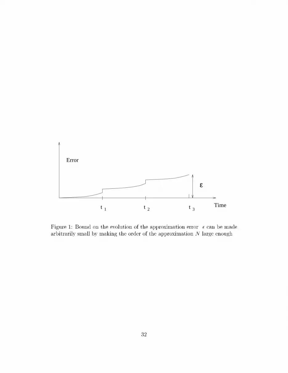
to computing FFT's and IFFT's. Before doing so, we address the convergenceof the Nonlinear Projection Filter.4 ConvergenceIn this section, we state conditions that guarantee that the Nonlinear Pro-jection Filter (NPF) given by Equations (10) and (11), converges (in the L2norm) to the exact nonlinear �lter given by Equations (3) and (4). The essenceof the proof is to show that the bound on the estimation error is given by agraph that looks like Figure 1. The evolution of the error between the Galerkinapproximation and the actual nonlinear �lter is bounded by the curve, where� can be made arbitrarily small by making the number of approximating termsN large. The bound on the error grows exponentially in between each sam-pling period and then jumps a �nite amount at each measurement update. Wenote that the bound derived in this section and depicted in Figure 1, is veryconservative.To make the convergence arguments transparent, we introduce some specialnotation that will only be used in this section. Assume that � Rn is a closedand bounded subset of Rn and let p̂ be the truncation of p to , i.e.p̂(t; x) = 8>>>><>>>>:p(t; x) if x 2 0 otherwise :We assume that p is integrable, which implies that for every � > 0, there exist12

a closed and bounded set � Rn such that kp� p̂kL2 < �, for all t 2 [t0; t1).We write the Kolmogorov equation as@p@t + L(p) = 0;where L(p) 4= nXi=1 @(pfi)@xi � 12 nXi=1 nXj=1 @2[p(GQGT )ij]@xi@xj :We assume that the basis functions f�`g1̀=0 form a complete basis for L2()and that R L(�j)�kdx < 1 for all (j; k). Using arguments similar to thoseoutlined in,18 we can assume, without loss of generality, that the basis functionsf�`g1̀=0 are orthonormal on the set . This assumption is made to simplify theconvergence proof, but does not impose a practical limitation on the selectionof the basis functions. Practically, the basis functions are only required to belinearly independent.Since p̂ 2 L1 \ L2 it has a Fourier expansion, which we denote asp̂(t; xjYt) = 1X̀=0 b`(t)�`(x): (14)Since for each t in the interval of interest, p̂ satis�es Kolmogorov's equationon , we get thatZ @(p̂ � pN)@t + L(p̂ � pN)!�qdx = 0;q = 0; : : : ; N � 1. Using equations (14) and (5) we get thatN�1X̀=0 (_b` � _c`) Z �`�qdx + N�1X̀=0 (b` � c`) ZL(�`)�qdx = � 1X`=N _b` Z �`�qdx� 1X`=N b` Z L(�`)�qdx;13

q = 0; : : : ; N�1. De�ne bN = (b0; : : : ; bN�1)T and �N = (�0; : : : ; �N�1)T . Us-ing the orthonormality of the basis functions and using the previously de�nedquantity AN , we obtain,( _bN � _cN) +AN(bN � cN) = � 1X`=N b` Z L(�`)�Ndx: (15)De�ne �N = 1X`=N b` ZL(�`)�Ndx :The following theorem states the main result of this section.Theorem 4.1 If the assumptions described above hold, and if�NkANkekANk ! 0; as N ! 0;then given a �xed time t̂ > 0, and any � > 0, there exists a K such that forN > K, kp(t; xjYt)� pN (t; xjYt)kL2 < � for all t < t̂.The proof to this theorem is made transparent by the following three lem-mas.Lemma 4.2 Under the hypothesis of Theorem 4.1, for any � > 0, there existsa positive integer K and a �k > 0 such that if N > K and kbN (tk)� c(tk)k <�k, then kbN (t)� c(t)k < �, for all t 2 [tk; t�k+1).Proof: Since the di�erential equation _� = �AN� is globally Lipschitz withLipschitz constant kANk, the theorem on the continuous dependence of ordi-nary di�erential equations on initial conditions and bounded disturbances,2114

and equation (15), imply thatkbN (t)� cN(t)k � �kekANk(t�tk) + �NkANk(ekANk(t�tk) � 1): (16)The �rst term can be made less than �=2 by making�k < �2e�kANk(t�k+1�tk):The hypothesis of Theorem 4.1 implies that there exist a K such that N > Kimplies that the second term is less than �=2. Q.E.D.Lemma 4.3 Under the hypothesis of Theorem 4.1, for any � > 0, there existsa positive integer K and a ��k+1 > 0 such that if N > K and bN(t�k+1)� cN(t�k+1) <��k+1, then kbN (tk+1)� cN(tk+1)k < �.Proof: Equation (11) shows thatc(tk+1) = M�1�(yk+1)c(t�k+1)�(yk+1)Tc(t�k+1) : (17)If we truncate equation (4) to and integrate we obtainb(tk+1) = M�1�(yk+1)b(t�k+1) + �1N�(yk+1)Tb(t�k+1) + �2N + �3N ; (18)where �1N = Z 1X`=N b`p(yk+1j�)�`(�)�N(�)d�;�2N = Z 1X`=N b`p(yk+1j�)�`(�)d�;�3N = Z 1X`=N b`�(�)d�:15

Since the Fourier series converges, k�1Nk, j�2N j and k�3Nk can be made lessthan any arbitrary positive number for N su�ciently large.Subtracting equation (18) from equation (17) we obtainkbN (tk+1)� cN(tk+1)k� M�1�b(t�k+1)�Tb(t�k+1) + �2N � M�1�c(t�k+1)�Tc(t�k+1) + �1N�Tb(t�k+1) + �2N + k�3Nk :De�ne � 4= 1�Tb(t�k+1) + �2N�N 4= 1�Tc(t�k+1) :Using this notation we have the following sequence of inequalities: M�1�b(t�k+1)�Tb(t�k+1) + �2N � M�1�c(t�k+1)�Tc(t�k+1) = �M�1�b(t�k+1)� �NM�1�c(t�k+1) � M�1� �b(t�k+1)� �Nc(t�k+1) = M�1� �(b(t�k+1)� c(t�k+1))+ (�� �N)c(t�k+1) � M�1� hj�j b(t�k+1)� c(t�k+1) + j�� �N j c(t�k+1) i :Since p(yk+1jx) is a Gaussian density we know that kM�1�(yk+1)k = B1 <116

and j�j = B2 < 1. We also know that c(t�k+1) = B3 < 1, where B1, B2and B3 are �nite numbers.Also note thatj�� �N j = ����� 1�Tb(t�k+1) + �2N � 1�Tc(t�k+1) ������ �(�Tb(t�k+1) + �2N )(�Tc(t�k+1)) � bN(t�k+1)� cN(t�k+1) + ����� �2N(�Tb(t�k+1) + �2N )(�Tc(t�k+1)) ����� :The �rst quantity is bounded above by a �nite number B4, and the secondquantity is a sequence, say �4N that converges in N . Thereforej�� �N j � B2 bN(t�k+1)� cN(t�k+1) + �4N :Collecting the above results we get thatkbN (tk+1)� cN(tk+1)k� B1 hB2 bN(t�k+1)� cN(t�k+1) + (B4 bN(t�k+1)� cN(t�k+1) + �4N )B2i + �3N + �5N ;where �5N = �1N�Tb(t�k+1) + �2N :The lemma follows from this formula. Q.E.D.17

Lemma 4.4 If at a particular instant of time t,kbN(t)� cN(t)k ! 0as N !1, then kp̂(t; xjYt)� pN(t; xjYt)kL2 ! 0:Proof: kp̂ � pNk2L2 = Z jp̂ � pN j2 dx� Z j(bN � cN)�N j2 dx+ Z ����� 1X`=N b`�`�����2 dx=(bN � cN)TM(bN � cN)+ Z ����� 1X`=N b`�`�����2 dx:By the mean value theorem of calculus, there exists a � 2 such thatkp̂ � pNk2L2 � kbN � cNk2 + �() ����� 1X`=N b`�`(�)�����2 ;where �() is the Lebesgue measure of . Since the second term on the righthand side is the tail of a convergent Fourier series, it converges to zero. Thelemma then follows from the hypothesis on kbN � cNk. Q.E.D.Proof of Theorem 4.1: First note thatkp� pNkL2 � kp� p̂kL2 + kp̂ � pNkL2 :Since an appropriate choice of guarantees that kp� p̂kL2 < �=2 for all t < t̂,18

we need to show that kp̂ � pNkL2 < �=2 for all t < t̂.Given tk < t̂ � tk+1 and �, Lemma 4.4 indicates that there exists a �̂such that if bN (t̂)� cN(t̂) < �̂, then p(t̂; xjYt̂)� pN (t̂; xjYt̂) L2 < �=2.From Lemma 4.2, there exists a Kk and a �k such that if N > Kk andkbN(tk)� c(tk)k < �k then bN(t̂)� cN(t̂) < �̂. From Lemma 4.3, thereexist a K�k and a ��k such that if N > K�k and bN (t�k )� cN(t�k ) < ��k thenkbN(tk)� c(tk)k < �k. Another application of Lemma 4.2 implies that thereexist a Kk�1 and a �k�1 such that if N > Kk�1 and if kbN(tk�1)� c(tk�1)k <�k�1 then bN(t�k )� cN(t�k ) < ��k .The above argument is repeated k times, resulting in the requirement thatkbN(0)� cN(0)k < �0. If we assume that the basis functions are orthonormal,then at time t = 0 there is zero approximation error sincep̂(0; xjY0) = p0(x)and Z pN(0; tjY0)�Ndx = Z p0(x)�Ndximplies that kbN(0)� cN(0)k = 0:Therefore letting K = max0�`�kfK`; K�̀g19

proves the theorem. Q.E.D.Remark 1. The bound derived in the above proof is given qualitatively byFigure 1.Remark 2. The requirement in the hypothesis of Theorem 4.1 that (�N= kANk)ekAk !0 is somewhat unsatisfactory since it is not clear at this stage how to guar-antee that this is true a priori. The requirement, however, can be tested forany given system. Further research could focus on deriving conditions underwhich this hypothesis holds.Remark 3. The convergence proof given in this section does not give explicitbounds on the approximation error. In other words, given a desired �, wecannot say what K must be to guarantee that an approximation error of � isachieved. We can only say that such a K does in fact exist.Remark 4. The convergence proof guarantees a small approximation errorfor any �nite time. The arguments given in this section do not say anythingabout the steady state error.5 Fourier BasisIn this section we show how to implement Equations (10) and (11) using aFourier basis and the FFT algorithm. Since the general n dimensional caseis notationally messy and the basic ideas are contained in one dimension, wewill restrict ourselves to this case. 20

Suppose we choose = [a; b] and a Fourier basisf `(x); !`(x)gN�1`=0 = ( 1pb� a cos 2�`b� a(x� a)! ; 1pb� a sin 2�`b� a(x� a)!)N�1`=0 :Note that the complex exponential basis is �` = ` + j!`. If a` and b` are theFourier coe�cients, and c` = a` � jb`, thenpN(x; tjYt) = N�1X̀=0 a`(t) `(x) + b`(t)!`(x)= 12 N�1X̀=0 c`(t)�`(x) + c�̀(t)��̀(x)= <(N�1X̀=0 c`(t)�`(x)) :We will therefore work with a complex exponential basis function, taking thereal part when we require an output of the �lter.The FFT algorithm can be used to approximate the inner product of twocomplex functions of x as follows:Z ba �(x)��k(x)dx � pb� aN FFTk [�(�)] ; (19)where the input to the FFT algorithm (denoted by �) is N uniform samples of� over the interval [a; b]. Therefore, the FFT returns N weighted integrals of�. Using Equation (19), we can use the FFT to approximate Equations (7){(9)and (12){(13) asM =I[A1(t)]` =pb� aN FFT " j 2�`b� af(�) + @f@x! (�)!�`(�)#21

[A2(t)]` =pb� aN FFT "Q2 @2[�`G2]@x2 ! (�)#s =pb� aN FFT [p(t0; �)][�k]` =pb� aN FFT [p(ykj�)�`(�)]�(yk) =pb� a IFFT [p(ykj�)] :The IFFT is used in the last equation since Equation (13) is an inner productwith �� instead of � (inner product is de�ned with a conjugation). Theseequations show that all of the quantities needed to propagate c(t) betweenmeasurements and to update it at a measurement can be computed quicklyusing the FFT. Furthermore, �(yk) as computed above is a real symmetricToeplitz matrix. Therefore, we only need to compute its �rst column. Further-more, because of the structure of �(yk), the product �(yk)c is a convolutionand can be implemented in O(N logN) operations rather than O(N2) for thefull matrix vector product. Hence, the measurement update is an O(N logN)operation.As the output of our �lter we may wish to compute the conditional mean,the conditional covariance or the density function itself. These quantities canalso be computed e�ciently using the FFT as shown below.The Conditional Mean: By de�nition the conditional mean of the stateat time t based on observations up to and including time � � t is�x�t = Z �p(�; tjY�)d�22

We may compute the mean of our approximate conditional density as follows�̂x�t = Z �pN(�; tjY�)d�= Z �<(N�1X̀=0 c`(t)�`(�)) d�= <(N�1X̀=0 c`(t) Z x��̀ dx)= <f Tcg;where = pb� aIFFT [�]The Conditional Covariance: The covariance of the approximate condi-tional density function isP̂ �t = Z �2p̂N (�; tjY�)d� � (�̂x�t )2= <(N�1X̀=0 c`(t) Z x2��̀ dx� ( Tc)2)= <f�Tc� ( Tc)2g;where � = pb� aIFFT [�2].The Density Function: To recover the approximate density function itselfwe have pN(x; tjYt) = <(N�1X̀=0 c`(t)�`(x))= Npb� a<fIFFT[c(t)]g :23

6 ExamplesIn this section we give simulation results comparing the Nonlinear Projec-tion Filter (NPF) to the extended Kalman �lter (EKF) for three continuous-discrete �ltering scenarios: (1) a standard nonlinear �ltering problem, (2) amodel mismatch problem and (3) an unobservable bimodal system. In allthree scenarios the EKF and the NPF have the same initial conditions andparameters. For comparison, state estimates are plotted with the true statetrajectory.6.1 Nominal ExampleThis scenario compares the performance of the EKF and NPF for a standard�ltering problem. The system dynamics and output equation are given bydxt = sin�x(t) + �18� dt+ d�tyk = x3(tk) + vk;where Q = 0:5 and R = 0:5. The sampling period is T = 0:001 seconds. Theinitial state and the initial state estimate are both set to zero. The initialcovariance estimate is one. The approximation interval is = [�10; 10] andthe number of Fourier basis elements is N = 64. Figure 2 shows the true statetrajectory as well as the estimated state trajectories produced by the NPF andEKF. As a �gure of merit, the RMS errors between the true and estimatedstates is 1.45 for NPF and 6.88 for the EKF. Figure 2 shows that most of the24

error occurs in the �rst 15 iterations. The NPF converges much faster than theEKF. However, after convergence, they both give very good state estimates.6.2 Model MismatchIn this scenario, the �lters were given an erroneous mathematical descriptionof the system dynamics. First, the �lters were given a linear dynamic modelfor the system with a nonlinear measurement equationdxt = xtdt+ d�tyk = x3tk + vk;But, the true dynamics were actually nonlinear:dxt = xt + x3t10 + d�tyk = x3tk + vk:The simulation parameters are identical to the previous section. The statetrajectories are shown in Figure 3 where the RMS error for the NPF is 1.14,and the RMS error for the EKF is 22.36. The key point is that the EKF seemsto be diverging from the true state while the NPF gives quality estimates evenin the presence of a model mismatch.25

6.3 An Unobservable SystemAs a last example, consider the systemdxt = �x3t + xt + d�t (20)yk = x2tk + vk: (21)In the absence of noise, system (20) has three equilibria: an unstable equi-librium at xt = 0, and two stable equilibria at xt = �1. In the presence ofnoise xt will evolve around either �1. The interesting thing is that the outputcannot be used to distinguish the two equilibria �1. Since we cannot distin-guish �1 we expect that the conditional density function for the state will bebimodal with major lobes centered at �1. It is interesting to note that themean of such a distribution will be zero. Therefore if the initial condition ofthe EKF is a zero mean Gaussian, then the EKF will always return a mean ofzero: a useless result. The EKF for this problem is given bydx̂dt = �x̂3 + x̂_P = �6x̂2 � 2 +QKk = 2P�(tk)x̂�k4x̂�2k P�(tk) +RP (tk) = (1� 2Kkx̂�k )P�(tk)x̂k = x̂�k +Kk(yk � x̂�k ):From the prediction equation we can see that the EKF has three equilibriaas well. Which equilibria the �lter predicts as the state will depend on the26

initial condition x̂(0). We have already noted that if x̂(0) = 0 then x̂(t) � 0for all t � 0. However, in this case the covariance diverges which indicatesthat the �lter is not working. If x̂(0) > 0(< 0) then x̂(t) ! +1(�1) and thecovariance converges to zero. If the initial state of the system is zero then thenoise during the initial transients of the system will determine whether thesystem goes to �1. It is therefore impossible to predict a priori the sign withwhich we should initialize the EKF.To our knowledge, there is no existing �lter (other than the Nonlinear Pro-jection Filter) that can return the correct density function for this system. Theoutput of the Nonlinear Projection Filter is shown in Figure 4. The thin linesare the density function returned by the NPF at the measurement updates.The heavy line is the actual state of the system. The NPF is initialized witha zero mean Gaussian. The �rst thin line is a Gaussian distribution. Afterone measurement the predicted density function is bimodal with modes ap-proximately centered at plus and minus the absolute value of the actual state,which is what we expect.7 ConclusionsIn this paper we have used the Galerkin spectral method to derive a nonlinear�lter that approximates the exact evolution of the conditional density functionof a nonlinear system. We have shown that our �lter converges to the truedensity function as the order of the approximation is increased. We have also27

shown how to use the FFT algorithm to e�ciently implement the algorithmand demonstrated several simple examples where our �lter outperforms theEKF. The results contribute to the state-of-the-art in nonlinear �ltering byderiving an approximate �lter that returns the entire density function andis not based on the linearization of the system. We should also note thatvarious �lters other than the minimum variance �lter could be derived fromour approximation since we approximate the conditional density on the stateand not its moments. We should note that our �lter su�ers from the \curseof dimensionality" in that the projection equations must be implemented overan n dimensional state space. This, however, is an inherent property of exactnonlinear �ltering and will be present in any approximation scheme.AcknowledgmentWe would like to acknowledge the contributions of Jay Wilson and TravisOliphant to the development of this paper. We also acknowledge John Kennyfor his helpful discussions and comments.References1 R. E. Kalman, \A new approach to linear �ltering and prediction problems,"Transactions of the ASME Journal of Basic Engineering, vol. 82, pp. 34{35,28

1960.2 R. E. Kalman and R. S. Bucy, \New results in linear �ltering and predictiontheory," Transaction of the ASME Journal of Basic Engineering, vol. 83,pp. 95{108, 1961.3 A. H. Jazwinski, Stochastic Processes and Filtering Theory, vol. 64 ofMath-ematics in Science and Engineering. New York, New York: Academic Press,Inc., 1970.4 H. J. Kushner, \Dyanamical equations for optimal nonlinear �lter," Journalof Di�erential Equations, vol. 3, pp. 179{190, 1967.5 H. J. Kushner, \Nonlinear �ltering: The exact dynamical equations satis-�ed by the conditional mode," IEEE Transactions on Automatic Control,vol. 12, pp. 262{267, 1967.6 R. L. Stratonovich, \Conditional Markov processes," Theory of Probabilityand its Applications, vol. 5, pp. 156{178, 1960.7 A. E. Bryson and Y. C. Ho, Applied Optimal Control. New York, New York:Hemisphere, 1975.8 F. L. Lewis, Optimal Estimation: With an Introduction to Stochastic Con-trol Theory. New York, New York: John Wiley & Sons, 1986.29

9 R. F. Ohap and A. R. Stubberud, \A technique for estimating the state of anonlinear system," IEEE Transactions on Automatic Control, pp. 150{155,April 1965.10 A. Gelb, ed., Applied Optimal Estimation, ch. 6. Cambridge, MA 02142:The M.I.T. Press, 1974.11 S. G. Mikhlin, Variational Methods in Mathematical Physics. New York,New York: MacMillan Company, 1964.12 L. V. Kantorovich and V. I. Krylov, Approximate Methods of Higher Anal-ysis. New York, New York: Interscience Publishers, Inc., 1958.13 F. H. Ling and X. X. Wu, \Fast Galerkin method and its application to de-termine periodic solutions of non-linear oscillators," International Journalof Non-Linear Mechanics, vol. 22, no. 2, pp. 89{98, 1987.14 R. Bouc and M. De�lippi, \A Galerkin multiharmonic procedure for non-linear multidimensional random vibration," International Journal of Engi-neering Science, vol. 25, no. 6, pp. 723{733, 1987.15 H. Weber, \Numerical solution of a class of nonlinear boundary value prob-lems for analytic functions," Journal of Applied Mathematics and Physics,vol. 33, pp. 301{314, May 1982.16 R. Beard, Improving the Closed-Loop Performance of Nonlinear Systems.PhD thesis, Rensselaer Polytechnic Institute, Troy, New York, 1995.30

17 R. Beard, G. Saridis, and J. Wen, \Improving the performance of stabilizingcontrol for nonlinear systems," Control Systems Magazine, vol. 16, pp. 27{35, Oct. 1996.18 R. Beard, G. Saridis, and J. Wen, \Galerkin approximation of the general-ized Hamilton-Jacobi-Bellman equation," Automatica. A Journal of IFAC,the International Federation of Automatic Control, vol. 33, pp. 2159{2177,Dec. 1997.19 R. Beard, G. Saridis, and J. Wen, \Approximate solutions to the time-invariant Hamilton-Jacobi-Bellman equation," Journal of OptimizationTheory and Applications, vol. 96, March 1998.20 E. Zeidler, Nonlinear Functional Analysis and its Applications, II/A: LinearMonotone Operators. Berlin, Germany: Springer Verlag, 1990.21 H. K. Khalil, Nonlinear Systems, p. 85. New York, New York: MacmillanPublishing Company, 1992.

31

t 1 t 2 t 3

ε

Error

TimeFigure 1: Bound on the evolution of the approximation error. � can be madearbitrarily small by making the order of the approximation N large enough.

32

True

GF

EKF

0 10 20 30 40 50 60−2

−1

0

1

2

3

4

5

6

Figure 2: Standard Filtering Problem: A comparison of state trajectory es-timates of an Extended Kalman Filter and the Nonlinear Projection Filter.Points are plotted at observation times.33

True

GF

EKF

0 10 20 30 40 50 60−2

0

2

4

6

8

10

Figure 3: Model Mismatch Problem: A comparison of state trajectory es-timates of an Extended Kalman Filter and the Nonlinear Projection Filter.Points are plotted at observation times.34

True State

time

xFigure 4: Approximate density function and the true state at the measurementupdates.35