A finite characterization of weak lumpable Markov processes. Part I: The discrete time case

A Finite Characterization of

Weak Lumpable Markov Processes�

Part I� The Discrete Time Case�

Gerardo Rubino and Bruno Sericola

IRISA � INRIA

Campus de Beaulieu� �� Rennes Cedex� FRANCE

Abstract

We consider an irreducible and homogeneous Markov chain �discrete time� with �nite

state space� Given a partition of the state space� it is of interest to know if the aggregatedprocess constructed from the �rst one with respect to the partition is also Markov homo�

geneous� We give a characterization of this situation by means of a �nite algorithm� This

algorithm computes the set of all initial probability distributions of the starting homogeneous

Markov chain leading to an aggregated homogeneous Markov chain�

Markov Chains� Aggregation� Weak Lumpability

� Introduction

This paper is the natural continuation of the work performed in G� Rubino and B� Sericola ��

To remain compatible with this previous paper� we conserve the same notation� Let us �rst recall

the problem of weak lumping in Markov chains�

Let X � �Xn�n�� be a homogeneous irreducible Markov chain evolving in discrete time� The

state space is assumed to be �nite and denoted by E � f�� Ng� The stationary distribution

of X is denoted by �� Let us denote by B � fB�� B�� B�M�g a partition of the state space

and by n�m� the cardinal of B�m�� We assume the states of E ordered such that

B�� f�� n��g��

B�m� � fn�� n�m� �� n�� n�m�g��

B�M� � fn�� n�M � �� Ng�

�

With the given process X we associate the aggregated stochastic process Y with values in the set

F � f�� Mg� de�ned by

Yn � mdef�� Xn � B�m�� for all n � �

It is easily checked from this de�nition and the irreducibility of X that the process Y obtained is

also irreducible in the following sense� for all m � F � for all l � F such that IP�Y� � l� � �� there

exists n � � such that IP�Yn � m�Y� � l� � ��

The Markov property of X means that given the state in which X is at the present time�

the future and the past of the process are independent� Clearly� this is no longer true for the

aggregated process Y in the general case �see the example below�� This paper deals with the

conditions under which the process Y is also a homogeneous Markov chain�

The homogeneous Markov chain X is given by its transition probability matrix P and its

initial distribution � we shall denote it by �� P � when necessary� The �i� j� entry of matrix P

is denoted by P �i� j�� We shall denote by agg�� P�B� the aggregated process constructed from

�� P � over the partition B� Let us denote by A the set of all probability vectors with N entries�

Of course� it is possible to have the situation in which agg�� P�B� is a Markov homogeneous

chain for any � � A� This happens� for instance� in the following example where E � f�� g�

B�� f�g� B�� f� �g and

P �

�B� �� p p �q � �� qq �� q �

�CAwith � � p � � and � � q � �� In this case� X is said to be strongly lumpable with repect to the

partition B and this is a well known property with a simple characterization� For every i � E and

m � F � let us denote by P �i� B�m�� the transition probability of passing in one step from state

i to the subset B�m� of E� that is P �i� B�m��def�P

j�B�m� P �i� j�� Then� X is strongly lumpable

with respect to the partition B if and only if for every pair of elements l� m � F � the probability

P �i� B�m�� has the same value for every i � B�l�� This common value is the transition probability

from state l to state m for the aggregated homogeneous Markov chain Y �

The opposite situation in which for any initial distribution �� the process agg�� P�B� is

not Markov is illustrated by the following example� Consider again a three state chain with

B�� f�g� B�� f� �g and

P �

�B� �� p p ��

�CA �

For any value of p with � � p � � and for any initial probability distribution� we have

IP�Xn�� B�� j Xn � B�� Xn�� B��

and IP�Xn�� B�� j Xn � B�� Xn�� B��

In �� the authors show that a third situation is possible� in which there exists a proper subset of A

denoted here by AM such that for any � � AM� the process agg�� P�B� is Markov homogeneous

while for any � �� AM the aggregated process is not Markov� In this more general situation� X

is said to be weakly lumpable with respect to the given partition B �see �� for some examples��

Moreover� in the same reference a su�cient condition to weak lumpability is given�

In �� the authors analyse the problem of the characterization of weak lumpability� An inter�

esting technique is introduced but we have shown in G� Rubino and B� Sericola �� that their

characterization is wrong�

The work performed here is an extension of G� Rubino and B� Sericola �� We obtain

a �nite characterization of weak lumpability by means of an algorithm which computes the set

AM� In G� Rubino and B� Sericola �� AM is given as an in�nite intersection of sets� The

main result obtained in this paper is the reduction of this in�nite intersection to a �nite one�

�

The paper is organized as follows� The next section gives the background material and notation

and recalls the main results obtained in G� Rubino and B� Sericola �� In Section �� we show

how the searched set AM can be obtained by means of a �nite algorithm� Section � presents an

example in which the set AM is computed and Section � concludes the paper�

� Notation and main results of G� Rubino and B� Seri�

cola ��

By convention� the vectors will be row vectors� Column vectors will be indicated by means of the

transposition operator � � �T � A vector with all its entries equal to � will be denoted simply by �

its dimension will be de�ned by the context�

For each l � F and � � A we denote by Tl�� the �restriction� of � to the subset B�l�� That is�

Tl�� is a vector with n�l� entries and its ith entry is �Tl��i� � � �n�� n�l � �� i� � i �

�� n�l�� When Tl�� we denote by �B�l� the vector ofA de�ned by �B�l��i� � ��i��kTl��k

if i belongs to B�l�� otherwise� where k�k denotes the sum of the components of the non negative

real vector �� Each time when in the sequel we shall write a vector of the form �B�m� with � � A�

we implicitely mean that this vector is de�ned� i�e� Tm��

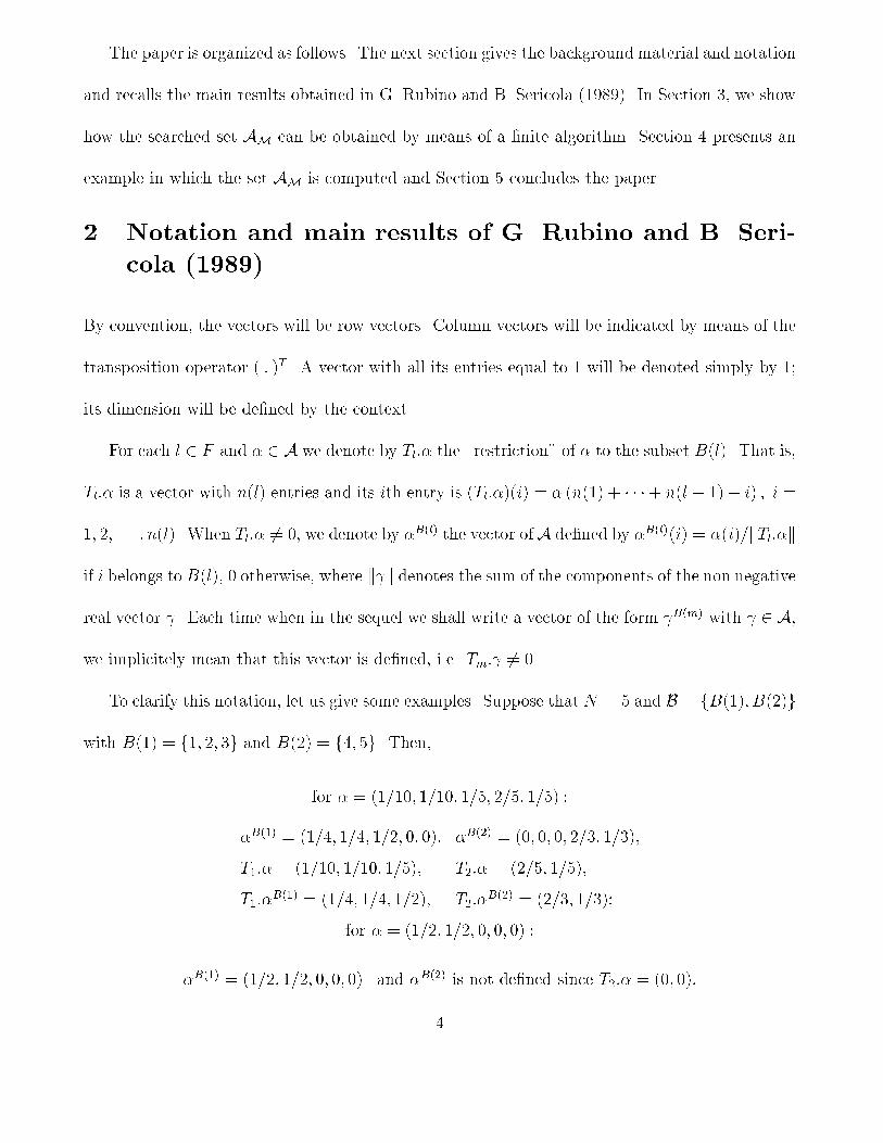
To clarify this notation� let us give some examples� Suppose that N � � and B � fB�� B��g

with B�� f�� g and B�� f�� g� Then�

for � � ��

�B�� B��

T�� T��

T��B�� T��

B��

for � � ��

�B�� and �B�� is not de�ned since T��

�

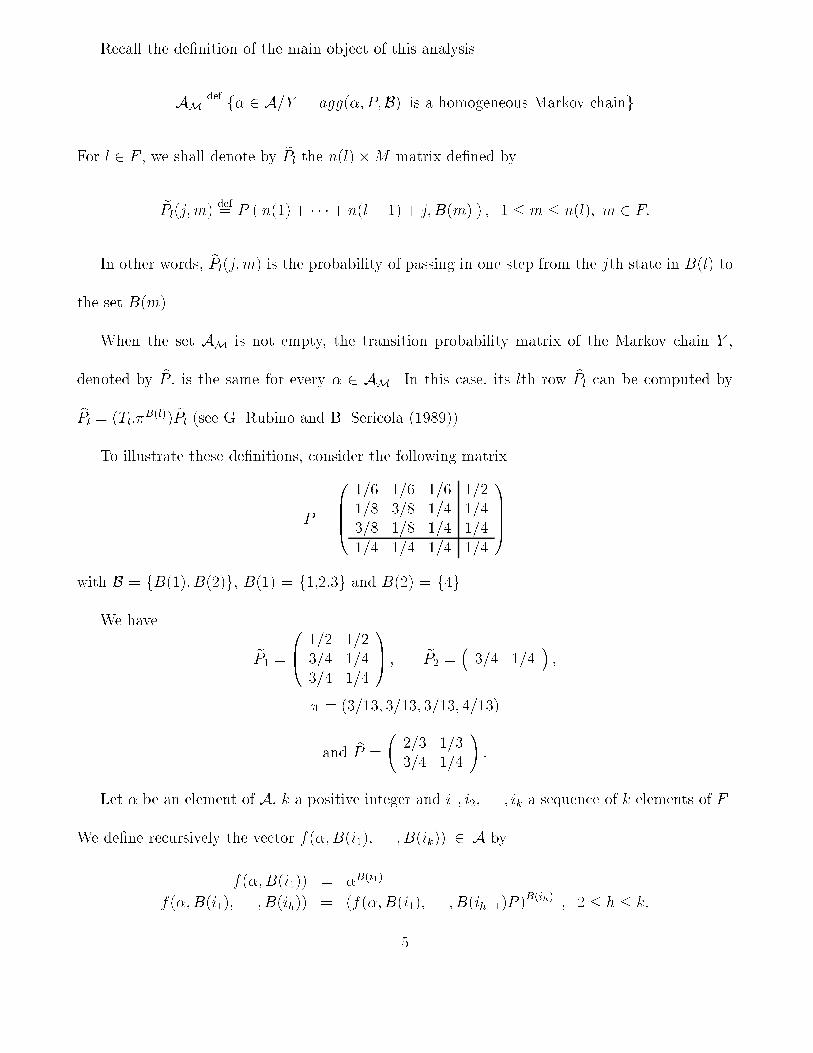
Recall the de�nition of the main object of this analysis�

AMdef� f� � A�Y � agg�� P�B� is a homogeneous Markov chaing

For l � F � we shall denote by ePl the n�l��M matrix de�ned by

ePl�j�m�def� P � n�� n�l � �� j� B�m� � � � � m � n�l�� m � F�

In other words� ePl�j�m� is the probability of passing in one step from the jth state in B�l� to

the set B�m��

When the set AM is not empty� the transition probability matrix of the Markov chain Y �

denoted by bP � is the same for every � � AM� In this case� its lth row bPl can be computed by

bPl � �Tl��B�l�� ePl �see G� Rubino and B� Sericola ��

To illustrate these de�nitions� consider the following matrix

P �

�BBB��

�CCCAwith B � fB�� B��g� B�� f��g and B�� f�g�

We have

eP� �

�B� ��

�CA � eP� ��

��

� � ��

and bP �

��

��

Let � be an element of A� k a positive integer and i�� i�� ik a sequence of k elements of F �

We de�ne recursively the vector f��B�i�� B�ik�� A by

f��B�i�� B�i��

f��B�i�� B�ih�� f��B�i�� B�ih��P �B�ih� � � h � k�

�

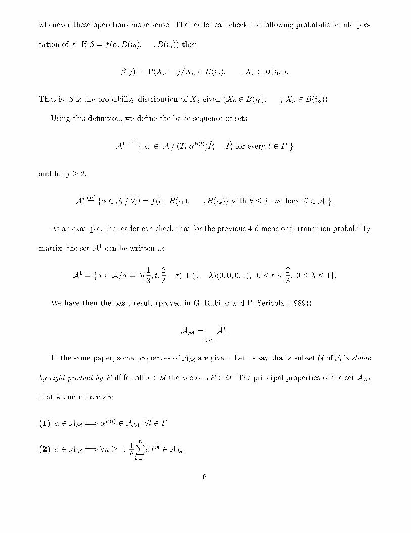
whenever these operations make sense� The reader can check the following probabilistic interpre�

tation of f � If � � f��B�i�� B�in�� then

��j� � IP�Xn � j�Xn � B�in�� X� � B�i��

That is� � is the probability distribution of Xn given �X� � B�i�� Xn � B�in��

Using this de�nition� we de�ne the basic sequence of sets

A� def� f � � A � �Tl��

B�l�� ePl � bPl for every l � F g

and for j � �

Aj def� f� � A � � � f�� B�i�� B�ik�� with k � j� we have � � A�g�

As an example� the reader can check that for the previous ��dimensional transition probability

matrix� the set A� can be written as

A� � f� � A��

�� t�

�� t� �� t �

�� g�

We have then the basic result �proved in G� Rubino and B� Sericola ��

AM ��j��

Aj�

In the same paper� some properties of AM are given� Let us say that a subset U of A is stable

by right product by P i� for all x � U the vector xP � U � The principal properties of the set AM

that we need here are

�� AM �� B�l� � AM� l � F

�� AM �� n � �� n

nXk��

�P k � AM

�

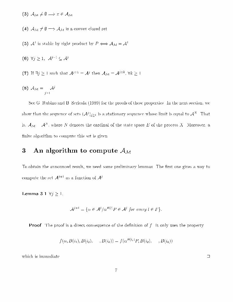
�� AM �� AM

�� AM �� AM is a convex closed set

�� A� is stable by right product by P �� AM � A�

�� j � �� Aj�� Aj

�� If �j � � such that Aj�� Aj then AM � Aj�k� k � �

�� AM ��j��

Aj

See G� Rubino and B� Sericola �� for the proofs of these properties� In the next section� we

show that the sequence of sets �Aj�j�� is a stationary sequence whose limit is equal to AN � That

is� AM � AN � where N denotes the cardinal of the state space E of the process X� Moreover� a

�nite algorithm to compute this set is given�

� An algorithm to compute AM

To obtain the announced result� we need some preliminary lemmas� The �rst one gives a way to

compute the set Aj�� as a function of Aj�

Lemma �� j � ��

Aj�� f� � Aj��B�l�P � Aj for every l � Fg�

Proof The proof is a direct consequence of the de�nition of f � It only uses the property

f��B�i�� B�i�� B�ik�� f��B�i��P�B�i�� B�ik��

which is immediate� �

�

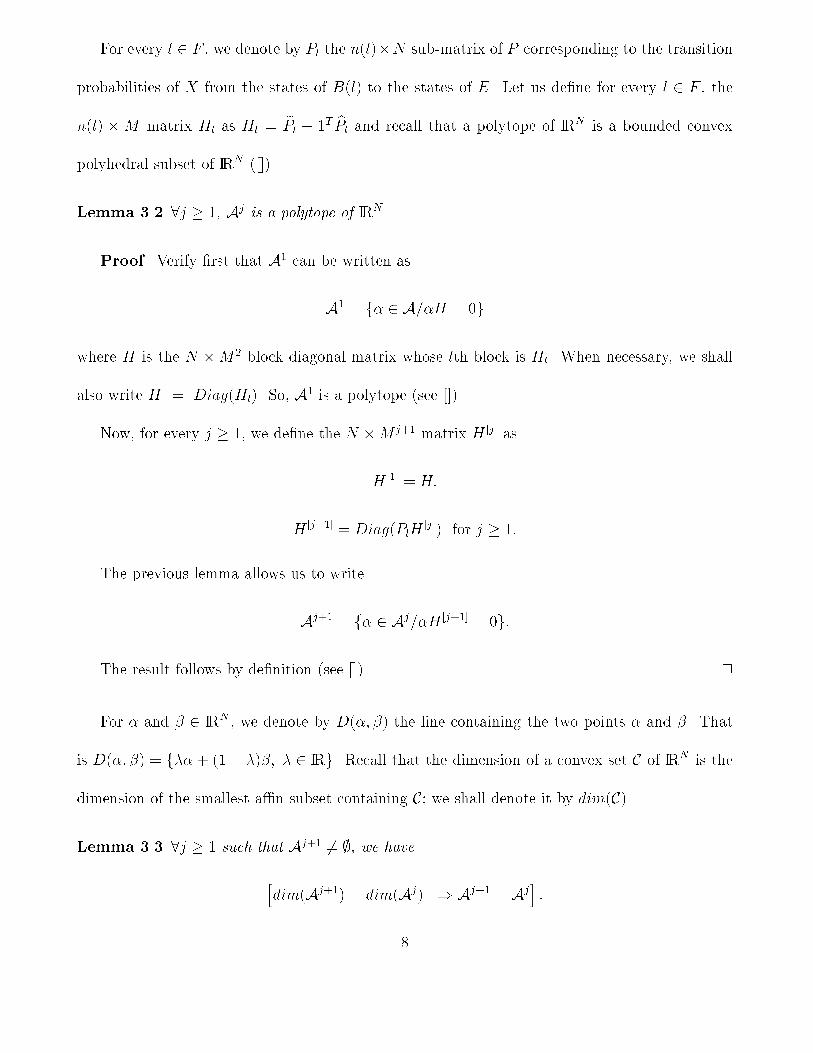
For every l � F � we denote by Pl the n�l��N sub�matrix of P corresponding to the transition

probabilities of X from the states of B�l� to the states of E� Let us de�ne for every l � F � the

n�l� �M matrix Hl as Hl � ePl � �T bPl and recall that a polytope of IRN is a bounded convex

polyhedral subset of IRN ��

Lemma �� j � �� Aj is a polytope of IRN �

Proof Verify �rst that A� can be written as

A� � f� � A��H � �g

where H is the N �M� block diagonal matrix whose lth block is Hl� When necessary� we shall

also write H � Diag�Hl�� So� A� is a polytope �see ��

Now� for every j � �� we de�ne the N �M j�� matrix H �j� as

H �� H�

H �j�� Diag�PlH�j�� for j � ��

The previous lemma allows us to write

Aj�� f� � Aj��H �j�� g�

The result follows by de�nition �see ��

For � and � � IRN � we denote by D�� the line containing the two points � and �� That

is D�� f� �� IRg� Recall that the dimension of a convex set C of IRN is the

dimension of the smallest a�n subset containing C we shall denote it by dim�C��

Lemma �� j � � such that Aj�� we have

hdim�Aj�� dim�Aj� ��Aj�� Aj

i�

�

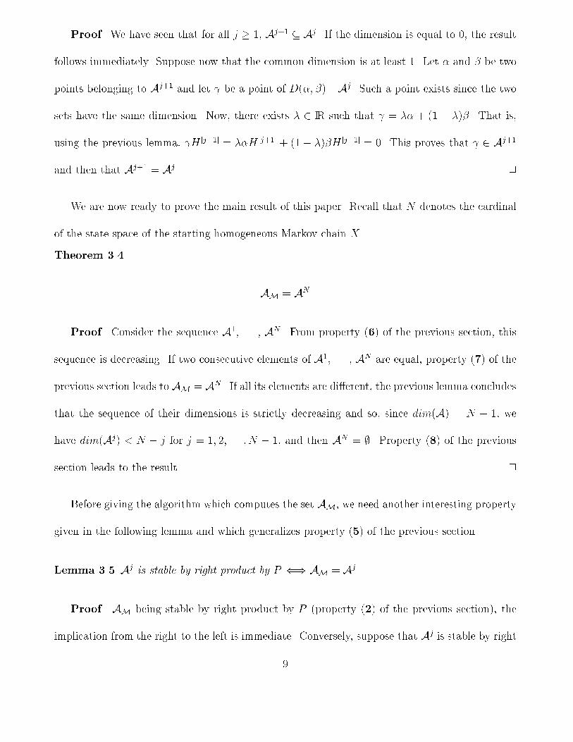
Proof We have seen that for all j � �� Aj�� Aj� If the dimension is equal to �� the result

follows immediately� Suppose now that the common dimension is at least �� Let � and � be two

points belonging to Aj�� and let � be a point of D�� Aj� Such a point exists since the two

sets have the same dimension� Now� there exists � IR such that � � � �� That is�

using the previous lemma� �H �j�� H �j�� H �j�� This proves that � � Aj��

and then that Aj�� Aj� �

We are now ready to prove the main result of this paper� Recall that N denotes the cardinal

of the state space of the starting homogeneous Markov chain X�

Theorem ��

AM � AN

Proof Consider the sequence A�� AN � From property �� of the previous section� this

sequence is decreasing� If two consecutive elements of A�� AN are equal� property �� of the

previous section leads to AM � AN � If all its elements are di�erent� the previous lemma concludes

that the sequence of their dimensions is strictly decreasing and so� since dim�A� � N � �� we

have dim�Aj� � N � j for j � �� N � �� and then AN � � Property �� of the previous

section leads to the result� �

Before giving the algorithm which computes the set AM� we need another interesting property

given in the following lemma and which generalizes property �� of the previous section�

Lemma �� Aj is stable by right product by P �� AM � Aj

Proof AM being stable by right product by P �property �� of the previous section�� the

implication from the right to the left is immediate� Conversely� suppose that Aj is stable by right

�

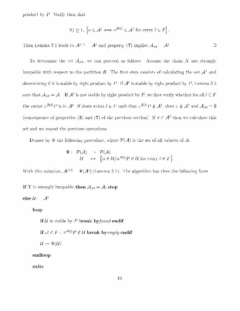
product by P � Verify then that

j � ��h� � Aj �� B�l� � Aj for every l � F

i�

Then Lemma �� leads to Aj�� Aj and property �� implies AM � Aj� �

To determine the set AM� we can proceed as follows� Assume the chain X not strongly

lumpable with respect to the partition B� The �rst step consists of calculating the set A� and

determining if it is stable by right product by P � If A� is stable by right product by P � Lemma ��

says that AM � A�� If A� is not stable by right product by P � we �rst verify whether for all l � F

the vector �B�l�P is in A�� If there exists l � F such that �B�l�P �� A�� then � �� A� and AM �

�consequence of properties �� and �� of the previous section�� If � � A� then we calculate this

set and we repeat the previous operations�

Denote by � the following procedure� where P�A� is the set of all subsets of A�

� � P�A� � P�A�

U ��n� � U��B�l�P � U for every l � F

oWith this notation� Aj�� Aj� �Lemma �� The algorithm has then the following form�

if X is strongly lumpable then AM � A stop

else U �� A�

loop

if U is stable by P break byfound endif

if �l � F � �B�l�P �� U break byempty endif

U �� U�

endloop

exits

��

exit found � AM �� U

exit empty � AM ��

endexits

endif

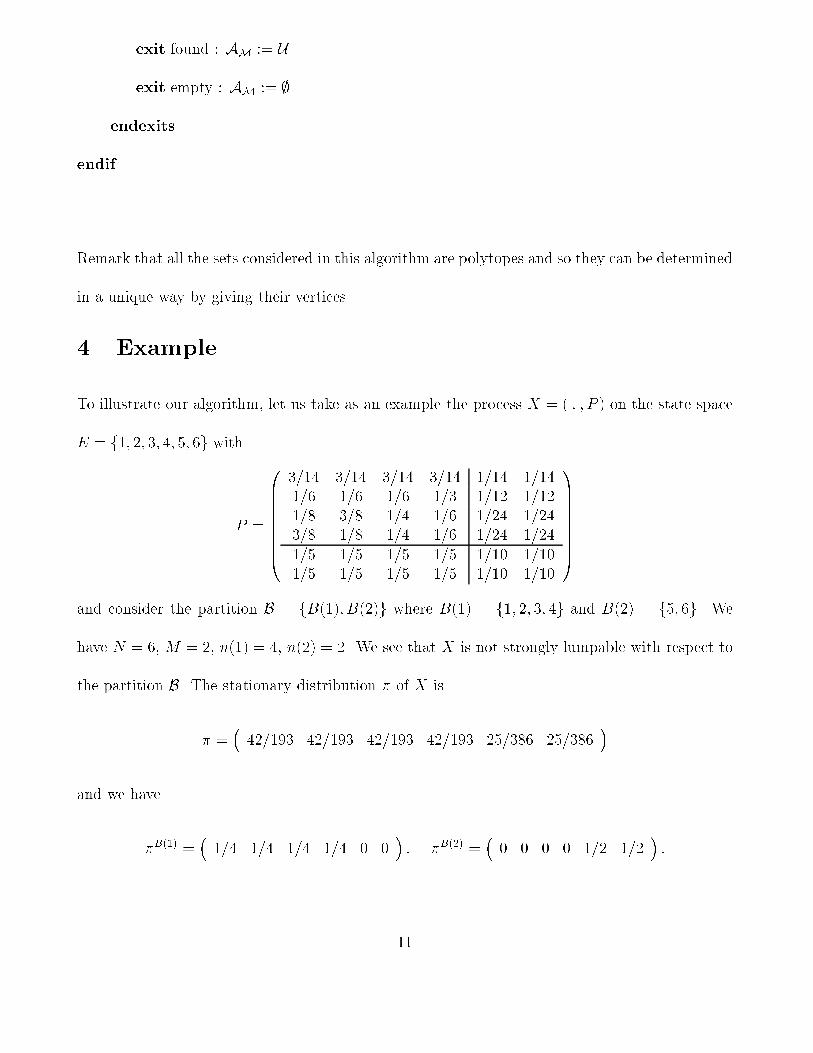
Remark that all the sets considered in this algorithm are polytopes and so they can be determined

in a unique way by giving their vertices�

Example

To illustrate our algorithm� let us take as an example the process X � � � � P � on the state space

E � f�� g with

P �

�BBBBBBBB�

��

�CCCCCCCCAand consider the partition B � fB�� B��g where B�� f�� g and B�� f�� g� We

have N � �� M � � n�� n�� We see that X is not strongly lumpable with respect to

the partition B� The stationary distribution � of X is

� ��

�

and we have

�B��

�� B��

��

��

��

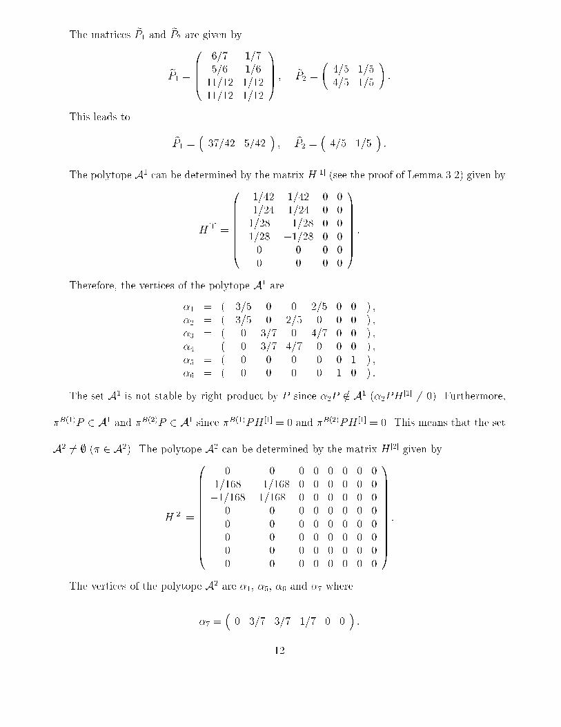
The matrices eP� and eP� are given by

eP� �

�BBB��

�CCCA � eP� �

��

��

This leads to

bP� ��

�� bP� �

��

��

The polytope A� can be determined by the matrix H �� see the proof of Lemma �� given by

H ��

�BBBBBBBB�

��

�CCCCCCCCA�

Therefore� the vertices of the polytope A� are

��

The set A� is not stable by right product by P since ��P �� A� ��PH�� Furthermore�

�B��P � A� and �B��P � A� since �B��PH �� and �B��PH �� This means that the set

A� �� A�� The polytope A� can be determined by the matrix H �� given by

H ��

�BBBBBBBBBBBBB�

� � � � � � � ��

� � � � � � � ��

�CCCCCCCCCCCCCA�

The vertices of the polytope A� are �� and � where

� ��

��

�

The set A� is not stable by right product by P since ��P �� A� ��PH�� Furthermore�

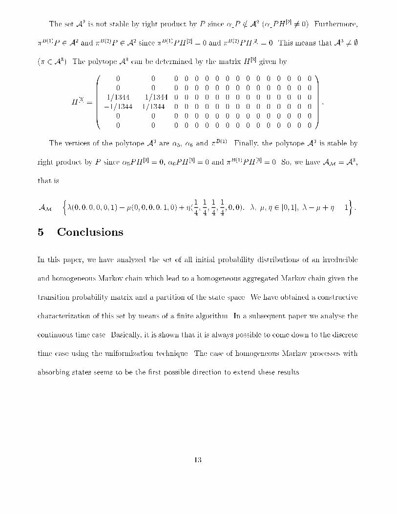
�B��P � A� and �B��P � A� since �B��PH �� and �B��PH �� This means that A ��

�� A�� The polytope A can be determined by the matrix H �� given by

H ��

�BBBBBBBB�

� � � � � � � � � � � � � � � ��

��

� � � � � � � � � � � � � � � ��

�CCCCCCCCA�

The vertices of the polytope A are �� and �B�� Finally� the polytope A is stable by

right product by P since ��PH�� PH

�� and �B��PH �� So� we have AM � A�

that is

AM ��

�

��

��

��

��

�

Conclusions

In this paper� we have analyzed the set of all initial probability distributions of an irreducible

and homogeneous Markov chain which lead to a homogeneous aggregated Markov chain given the

transition probability matrix and a partition of the state space� We have obtained a constructive

characterization of this set by means of a �nite algorithm� In a subsequent paper we analyse the

continuous time case� Basically� it is shown that it is always possible to come down to the discrete

time case using the uniformization technique� The case of homogeneous Markov processes with

absorbing states seems to be the �rst possible direction to extend these results�

��

References

�� A�M� Abdel�Moneim and F�W� Leysie�er� Weak lumpability in �nite Markov chains� J� Appl�

Prob� ��

�� J�G� Kemeny and J�L Snell� Finite Markov chains� Springer�Verlag� New York Heidelberg

Berlin� ��

�� R� T� Rockafellar� Convex Analysis� Princeton University Press� Princeton� New�Jersey� ��

�� G� Rubino and B� Sericola� On weak lumpability in Markov chains� J� Appl� Prob� � ��

��

��

Documents

A finite characterization of weak lumpable Markov processes. Part I: The discrete time case