A new approach based on discrete hidden Markov model using Rocchio algorithm for the diagnosis of the brain diseases

Digital Signal Processing 20 (2010) 923–934

Contents lists available at ScienceDirect

Digital Signal Processing

www.elsevier.com/locate/dsp

A new approach based on discrete hidden Markov model using Rocchioalgorithm for the diagnosis of the brain diseases

Harun Uguz ∗, Ahmet Arslan

Selcuk University, Eng.-Arch. Fac. Computer Eng., 42075-Konya, Turkey

a r t i c l e i n f o a b s t r a c t

Article history:Available online 11 November 2009

Keywords:Transcranial Doppler signalsDiscrete hidden Markov modelRocchio algorithmMaximum likelihood

Transcranial Doppler (TCD) study of the adult intracerebral circulation has gained animportant popularity in last 10 years, since it is a non-invasive, easy to apply and reliabletechnique. In this study, an implementation on biomedical system has been developedfor classification of signals gathered from middle cerebral arteries in the temporal areavia TCD for 24 healthy and 82 ill people which have one of the four different brainpatients such as; cerebral aneurysm, brain hemorrhage, cerebral oedema and brain tumor.Basically, the system is composed of feature extraction and classification parts. In thefeature extraction stage, the Linear Predictive Coding (LPC) Analysis and Cepstral Analysiswere applied in order to extract the cepstral and delta-cepstral coefficients in frame level asfeature vectors. In the classification stage a new Discrete Hidden Markov Model (DHMM)based approach was proposed for the diagnosis of brain diseases. This proposed methodwas developed via Rocchio algorithm. Therefore, to calculate DHMM parameters regulatedaccording to maximum likelihood (ML) approach, both training samples of related classand other classes were included in calculation. Thus, DHMM model parameters presentingone class were suggested to represent the training samples related to that class better aswell as not to represent the training samples related to other classes. The performanceof the proposed DHMM with Rocchio approach was compared with some methods suchas DHMM, Artificial Neural Network (ANN), neuro-fuzzy approaches and obtained betterclassification performance than these methods.

© 2009 Elsevier Inc. All rights reserved.

1. Introduction

The Doppler technique was introduced by Satomura in 1959. Since it is a non-invasive and safe method, its preference hasbeen increases gradually in last decade [1]. In 1982, Aaslid et al. introduced TCD ultrasonography. This method includes notonly recording of blood flow speed in intracranial arteries but also measurement of it [2]. The non-invasive TCD method hasa capable of evaluating the measurement of blood flow changes. Due to this property, TCD provides important informationin case of decrease in cerebral blood flow which often causes neurologic sequela. The reasons of its widely usage arebecause it is non-invasive, portable, easy to apply, reliable and tolerable technique as well as cheaper than other examinationmethods [3].

Many researches involving spectral analysis and classification have been introduced on TCD signals in the literature.Ozturk et al. used two different neuro-fuzzy classifiers to classify the chaotic invariant features extracted from the TCDsignals and compared the performance of the classifiers [4]. Serhatlıoglu et al. extracted the features with Fast FourierTransform (FFT) and classified these features using back propagation neural network and self-organizing map algorithms to

* Corresponding author. Fax: +90 332 241 06 35.E-mail addresses: [email protected], [email protected] (H. Uguz), [email protected] (A. Arslan).

1051-2004/$ – see front matter © 2009 Elsevier Inc. All rights reserved.doi:10.1016/j.dsp.2009.11.001

http://www.ScienceDirect.com/

http://www.elsevier.com/locate/dsp

mailto:[email protected]



http://dx.doi.org/10.1016/j.dsp.2009.11.001

924 H. Uguz, A. Arslan / Digital Signal Processing 20 (2010) 923–934

compare the performance of these classifiers [5]. Güler et al. improved a spectral analysis of TCD signals, based on FFT andadaptive autoregressive-moving average (A-Arma) methods. They also presented that A-Arma method is more effective thanFFT method [6].

In this study, TCD signals recorded from the middle arteries of the temporal region of brain of the 82 patients and 24healthy people were investigated. 20 of these people had cerebral aneurysm, 10 of them had brain hemorrhage, 22 of themcerebral oedema and 30 of them had brain tumor as in [4]. To classify TCD signals taken from 106 subjects, firstly featureextraction stage was implemented. At this phase, TCD signals were dived into the frames of equal length and windowingwas run on each frame to minimize the discontinuity. Afterwards, in order to extract the characteristic parameters of thesignal, 12 cepstral coefficients were obtained by applying LPC analysis and cepstral analysis, sequentially. At the last step offeature extraction stage, to eliminate dynamic information, 12 delta cepstrum coefficients were calculated from 12 cepstralcoefficients. Thus, 24 features were obtained for each frame consisting of 12 cepstral and 12 delta-cepstrum coefficients. Atthe last step, the features extracted from the TCD signals of four different groups of patients as well as healthy subjects areclassified with the DHMM-based classifiers.

Fundamental theory of the DHMM was invented by Baum et al. in the second half of 1960s [7–9]. The DHMM is adoubly stochastic process with an underlying stochastic process that is not observable, however it is observable via anotherset of stochastic process that create a sequence of observed symbols [10,11]. The DHMM has a wide application area such asautomatic speech recognition [12], gesture recognition [13,14], character recognition [15,16], and fault diagnosis system [17].

In this study, a new approach based on DHMM was suggested for the diagnosis of brain diseases. Rocchio algorithm wasadapted to the DHMM method as a novelty. Rocchio algorithm is a learning method which is one of the most known andhas a wide application area in the text mining [18]. This method was proposed to archive the aim of mining information infirst years and it is later applied to text classification. Based on this method and ML approach in regulation of the DHMMparameters (transition probability, observation symbol probability and initial state probability) belonging to each class, thetraining samples of that class as well as the training samples of other classes without that one have an important role.Main aim of this study is to regulate the DHMM parameters which represent related class better while separating that classfrom other classes better. Classification performance of new system was compared with the classification performance ofthe previous studies which were applied to same data set and superiority of new algorithm was demonstrated.

Remaining of this paper is organized as follows. Section 2 contains explanations about raw data obtaining, feature ex-traction techniques, Rocchio algorithm, DHMM classifier and fundamental theory of the proposed DHMM with Rocchioalgorithm classifier. The superiority of proposed classification system is experienced on TCD signals for diagnosing of braindiseases is described in Section 3. Finally in Section 4, conclusion and discussion part is presented.

2. Materials and methods

The parts of suggested biomedical system structure are explained in the following subsections:

2.1. Raw data obtaining

Various tools consist of 2 MHz transcranial Doppler unit (XX, DWL, GmbH, Uberlingen, Germany), an analog/digital (A/D)interface board and Personal Computer (PC) were used for raw data obtaining. The analog Doppler unit works in not onlycontinuous mode but also pulse wave mode. Ultrasonic transducer is run with an angle of 60◦ while TCD signals whichare recorded from middle cerebral arteries of the temporal measuring. The signal taken from blood vessel is sent to a PCthroughout a 16-bit sound card which is used as an analog/digital interface board.

2.2. Feature extraction

Since result of feature extraction affects the performance of classification, it is one of the most important steps inpattern recognition. In feature extraction processing, we aim to reduce the original waveform by eliminating useless partof the data. Reduced vector also includes most of the useful information from the original vector. Linear Predictive Coding(LPC) is preferred as a feature extraction method in this study because of the following reasons [19]:

• LPC provides a good model of the signal, giving a good approximation of the signal characteristic.• The LPC calculation method is simple and straightforward to implement in either software or hardware.

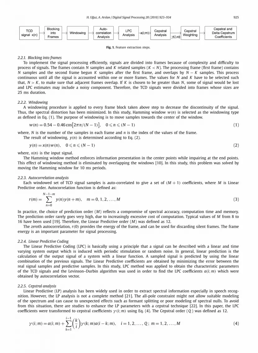
The steps of feature extraction processing can be seen in Fig. 1 [20]. According to Fig. 1, frame blocking step blocks thepreemphasized signal into frames. In order to minimize the signal discontinuities at the beginning and end of each frame,windowing step is applied. Autocorrelation analysis identifies the zeroth autocorrelation which is the energy of each framewhich is very important parameter. LPC parameter conversion to cepstral coefficients because of more reliable and robustthan the LPC coefficients. In order to add dynamic information, delta cepstrum coefficients are computed from cepstralcoefficients.

H. Uguz, A. Arslan / Digital Signal Processing 20 (2010) 923–934 925

Fig. 1. Feature extraction steps.

2.2.1. Blocking into framesTo implement the signal processing efficiently, signals are divided into frames because of complexity and difficulty to

process of signals. The frames contain N samples and K related samples (K < N). The processing frame (first frame) containsN samples and the second frame begun K samples after the first frame, and overlaps by N − K samples. This processcontinuous until all the signal is accounted within one or more frames. The values for N and K have to be selected suchthat, N > K , to make sure that adjacent frames overlap. If K is chosen to be greater than N , some of signal would be lostand LPC estimates may include a noisy component. Therefore, the TCD signals were divided into frames whose sizes are25 ms duration.

2.2.2. WindowingA windowing procedure is applied to every frame block taken above step to decrease the discontinuity of the signal.

Thus, the spectral distortion has been minimized. In this study, Hamming window w(n) is selected as the windowing typeas defined in Eq. (1). The purpose of windowing is to move samples towards the center of the window.

w(n) = 0.54 − 0.46 cos[2πn/(N − 1)

], 0 � n � (N − 1) (1)

where, N is the number of the samples in each frame and n is the index of the values of the frame.The result of windowing, y(n) is determined according to Eq. (2).

y(n) = x(n)w(n), 0 � n � (N − 1) (2)

where, x(n) is the input signal.The Hamming window method enforces information presentation in the center points while impairing at the end points.

This effect of windowing method is eliminated by overlapping the windows [10]. In this study, this problem was solved bymoving the Hamming window for 10 ms periods.

2.2.3. Autocorrelation analysisEach windowed set of TCD signal samples is auto-correlated to give a set of (M + 1) coefficients, where M is Linear

Predictive order. Autocorrelation function is defined as:

r(m) =N−1−m∑

n=0

y(n)y(n + m), m = 0,1,2, . . . , M (3)

In practice, the choice of prediction order (M) reflects a compromise of spectral accuracy, computation time and memory.The prediction order rarely goes very high, due to increasingly excessive cost of computation. Typical values of M from 8 to16 have been used [19]. Therefore, the Linear Predictive order (M) was defined as 12.

The zeroth autocorrelation, r(0) provides the energy of the frame, and can be used for discarding silent frames. The frameenergy is an important parameter for signal processing.

2.2.4. Linear Predictive CodingThe Linear Predictive Coding (LPC) is basically using a principle that a signal can be described with a linear and time

varying system output which is induced with periodic stimulation or random noise. In general, linear prediction is thecalculation of the output signal of a system with a linear function. A sampled signal is predicted by using the linearcombination of the previous signals. The Linear Predictive coefficients are obtained by minimizing the error between thereal signal samples and predictive samples. In this study, LPC method was applied to obtain the characteristic parametersof the TCD signals and the Levinson–Durbin algorithm was used in order to find the LPC coefficients a(i;m) which wereobtained by autocorrelation vector.

2.2.5. Cepstral analysisLinear Predictive (LP) analysis has been widely used in order to extract spectral information especially in speech recog-

nition. However, the LP analysis is not a complete method [21]. The all-pole constraint might not allow suitable modelingof the spectrum and can cause to unexpected effects such as formant splitting or poor modeling of spectral nulls. To avoidfrom this situation, there are studies to enhance the LP parameters with a cepstral technique [22]. In this paper, the LPCcoefficients were transformed to cepstral coefficients γ (i;m) using Eq. (4). The Cepstral order (Q ) was defined as 12.

γ (i;m) = a(i;m) +i−1∑(

k

i

)γ (k;m)a(i − k;m), i = 1,2, . . . , Q ; m = 1,2, . . . , M (4)

k=1


The cepstral sequence was weighted using the windowing function, wγ (i) shown in Eq. (5). The cepstral coefficientscalculated after weighting procedure were(was) shown in Eq. (6). After this procedure applied, 12 cepstral coefficients wereobtained.

wγ (i) = 1 + Q

2sin

(π i

Q

), i = 1,2, . . . , Q (5)

γw(i;m) = γ (i;m)wγ (i) (6)

In order to add dynamic information, Q different cepstral coefficients were computed using Eq. (7). 12 delta cepstrumcoefficients were obtained with this computation. Thus, an observation vector of 24 dimensions was obtained for eachframe. The observation vector was consisted of 12 cepstral and 12 delta cepstrum coefficients.

�γw (i;m) = 1

2

(γw(i;m + 1) − γw(i;m − 1)

), i = 1,2, . . . , Q ; m = 1,2, . . . , M (7)

2.3. Rocchio algorithm

Rocchio algorithm is a learning method which has the most popular and extensive application area in text mining [18].The method which was first developed for mining information is aimed to be a decision rule in the determination ofmemberships of documents in classes. The advantage of the method is that it is not depend on any threshold value. Thismethod is later adapted to text classification.

The basic idea of the algorithm is to represent each document d as a vector in a vector space so that documents withsimilar content have similar vectors. In this method, a prototype vector c j is formed to show each C j class in learning phase.Both the normalized document vectors of the positive samples for a class as well as those of the negative samples for a classare summed up [23]. The positive and negative samples represent relevant and irrelevant document vectors, respectively. Inthis way, all of the positive and negative training samples are included in training phase.

This method can be defined according to Eq. (8) [18].

C j = α1

|C j|∑d∈C j

−→d − β

1

|U − C j|∑

d∈|U−C j |

−→d (8)

where α and β represent the parameters adjusting the relative effects of positive and negative samples, respectively. U isthe number of documents in training data set, and d is the vector of training document. C j is the set of training documentsassigned to class j. As recommended in [23] α = 16 and β = 4. Nevertheless, the optimal values of α and β parameters arelikely to be task-dependent.

2.4. DHMM

A DHMM is a stochastic Finite State Machine (FSM). A DHMM is a double-layered finite state stochastic process, witha hidden Markovian process that controls the selection of the states of an observable process. In general a DHMM has Nstates, and transitions are available among the states. At different times, the system is in one of these states; each transitionbetween the states has an associated probability, and each state has an associated observation output (symbol). A DHMM ischaracterized by the followings [10]:

1. N , the number of states of the model. The set of individual states is denoted as S = {S1, S2, . . . , SN }, and state at timet as qt .

2. T , the number of observations. A typical observation sequence is denoted as

O = {O 1, O 2, . . . , O T } (9)

3. A = {aij}, the state transition probability distribution, of size N × N , defines the probability of transition from state i attime t , to state j at time t + 1.

aij = P (qt+1 = S j|qt = Si), 1 � i, j � N (10)

4. B = {b j(k)} ( j = 1, . . . , N; k = 1, . . . , C ) probability distribution of observation symbols for each state. b j is observationsymbol probability in state j. C is the number of the observation symbols.

5. The initial state distribution, π = {πi}, defines the probability of any given state.

πi = P (q1 = S j), 1 � i � N (11)

A complete specification of a DHMM requires specification of model parameters, specification of the three probabilitymeasures {A, B,π}. DHMM parameters use the following set:

λ = {A, B,π} (12)


Fig. 2. The training and recognition flow diagrams for DHMM.

The flow charts of training and recognition steps for DHMM are shown in Fig. 2. In the first step of DHMM training stage,the type of model and numbers of states are determined. All observation vectors that will be used in training of system areclustered in order to form codebook and C cluster centers are determined according to a clustering algorithm. The FuzzyC-Means (FCM) algorithm is one of the most widely used methods in clustering. In our study, FCM algorithm was usedclustering all observation vectors according to C cluster centers and each observation vector was assigned to a cluster. Thus,codebook process that deploys the FCM algorithm aims to reduce the sampled data for producing a sequence of observablevectors.

After this codebook forming stage, the distance of the observation vectors related to each class to C cluster centersare calculated according to Euclidean distance and it’s determined to which cluster each of this observation vectors be-long. DHMM model parameters (λ) belonging to each class are calculated iteratively by using Baum–Welch algorithm and


Fig. 3. General structure of the DHMM with Rocchio approach.

recorded in order to use in the recognition stage. The point that should be taken into consideration is to use observationvectors just belonging to that class during the calculation of DHMM model parameters of each class and to know that theobservation vectors of other classes do not affect the value of DHMM model parameters at calculation period. In the recog-nition stage, test sample is determined to which class it belongs by using recorded DHMM model parameters according toML approach [9].

As mentioned above, in the case of ML approach is used for computation of DHMM model parameters (λ), these param-eters are computed by using only the training samples of related class. The training samples not belonging to that class arenot used in the calculation of DHMM model parameters. The typical DHMM-based classification approach adopts the MLcriterion, where an unknown sequence O is assigned to the class showing the highest likelihood,

class(O ) = arg maxi=1,...,N

P (O |λi) (13)

where, λi is the DHMM corresponding to the ith class.

2.5. Suggested method

DHMM model parameters (λ) belonging to each class are calculated by using only the training samples of that class.The training samples not belonging to that class are not used in the calculation of DHMM model parameters. With theaim of supplying that deficiency, by involving the training samples of all classes to calculating processes, a new approach issuggested. In order to eliminate this deficiency in the calculation of DHMM model parameters, a new approach is formed. Inthe development of this approach, Rocchio algorithm is adapted to DHMM method. The most important property of Rocchioalgorithm is that the training samples (positive training samples) belonging to the class of which the parameters are calcu-lated as well as the training samples (negative training samples) belonging to other classes are used in the determination ofparameters. Thus, DHMM model parameters of one class represent to training samples of that class, while these parametersdo not represent to training samples not belonging to that class. Consequently, to use all training samples according to Roc-chio algorithm in the calculation of DHMM model parameters might have a positive effect in the success of classification.The general structure of the suggested approach is shown in Fig. 3.

In Fig. 3, DHMM module is same as the one used in the training stage in Fig. 2. Dissimilar from DHMM, DHMM modelparameters should be calculated independently from each other for the observation vectors presenting each of training sam-ples. Namely, different DHMM model parameters are calculated for each training sample belonging to related class. DHMMmodel parameters of each class are calculated from positive and negative components of that class. Positive components areDHMM model parameters of training samples belonging to that class. These values are summed and then divided by num-ber of positive training samples. Negative components, on the other hand, are DHMM model parameters of training samplesnot belonging to that class. These values are summed and divided by number of negative training samples. According toRocchio algorithm, DHMM model parameters of that class are determined by combining the positive and negative compo-nents with α and β parameters respectively (Eq. (14)). These procedures are repeated for each of the classes. Consequently,DHMM model parameter set which forms the classification model is found. In addition to this, it’s required to give 0 valuesto negative components of DHMM model parameters according to Rocchio algorithm.

λC j (A, B,π) = α1

|C j|∑

xk∈C j

λk(A, B,π) − β1

|U − C j|∑

xk∈|U−C j |λk(A, B,π) (14)

where α and β are the parameters adjusting the relative effects of positive and negative samples, respectively. λCi arethe DHMM model parameters of the class of Ci ; xk are the observation vectors representing kth training sample; λk arethe DHMM parameters calculated by using observation vectors which represent kth training sample; and U represents alltraining samples.

The recognition stage of the suggested method is same as the recognition steps of DHMM method seen in Fig. 2. Therewill be five separate log-likelihood values calculated for these classes of each test sample since there are five separateclasses for the subjects used in this study such as cerebral aneurism, brain hemorrhage, cerebral oedema, brain tumor, andhealthy subjects. In the decision stage, which class the test sample belongs to is decided according to ML approach. The


Table 1ANN architecture and training parameters.

ANN architectureThe number of layers : 3The number of neuron on the layers : Input : 24

Hidden : 50Output : 5

The initial weights and biases : The Nguyen–Widrow methodActivation functions : Log-sigmoid

ANN training parametersLearning rule : Back-propagationAdaptive learning rate : Initial : 0.0001

Increase : 1.05Decrease : 0.7

Momentum constant : 0.95Mean-squared error : 0.000001Max. Epoch (stopping criterion) 1000

Table 2Confusion matrix for the ANN classification results.

Output/desired Healthy Cerebral aneurism Brain hemorrhage Cerebral oedema Brain tumor

Healthy 12 0 0 0 0Cerebral aneurism 0 10 0 0 0Brain hemorrhage 0 0 4 0 1Cerebral oedema 0 0 0 8 3Brain tumor 0 0 0 0 16

more is the difference between calculated log-likelihood values for each class, the easier is the separation. For this reason,the training samples (positive training samples) belonging to the class, DHMM model parameters of which were calculatedin the training stage as well as the training samples belonging to other classes are also included in the calculation. It’schecked out that DHMM model parameters of each class will represent the related class better and better differentiationfrom other classes will be supplied. Crucial point in this study is to compute DHMM parameters using ML approach foreach class. In addition; since ML approach is used, only training samples of related class are used during computation whileDHMM parameters belonging to training samples of other classes are not effective in the computation.

3. Experimental results

3.1. Structure of data set

In this study, 106 different TCD signals recorded from 82 patients and 24 healthy subjects. Among 82 patients, 20 ofthem had cerebral aneurism, 10 patients had brain hemorrhage, 22 patients had cerebral oedema and the remaining 30patients had brain tumor. The group consisted of 52 males and 54 females with ages ranging from 3 to 65 years and amean age of 35.5 ± 0.5 years. 10 cerebral aneurism subjects, 5 brain hemorrhage subjects, 11 cerebral oedema subjects, 14brain tumor subjects and 12 healthy (normal) subjects were selected as training set. The remaining subjects were used fortesting. Thus, from 106 subjects 52 were separated as training set for the classifiers while 54 of them were used for testingas in [4].

3.2. Classification using artificial neural network

After feature extraction stage, the feature vectors belonging to the training set were used as input to the ArtificialNeural Network (ANN) classifier. The training parameters and the structure of the neural network used in this study wereshown in Table 1. This table summarizes the parameters such as the number of hidden layers, learning rate, momentumcoefficients and the types of activation functions which were changed to achieve the best classification performance. TheNeural Networks Toolbox of the Matlab software package was used for all the applications related with ANN.

After the training stage, the feature vectors belonging to the test set were applied as input to the trained ANN classifier.The confusion matrix showing the classification results of the ANN is given in Table 2.

According to the confusion matrix (Table 2), 3 subjects with cerebral oedema were incorrectly classified as brain tumorpatients and 1 subject with brain hemorrhage were incorrectly classified as a brain tumor patient.


Table 3DHMM and DHMM with Rocchio architectures.

DHMM DHMM with Rocchio

The best state numbers 9 8The best VQ size 9 5The best α value – 7The best β value – 3Evaluating problem solved Forward backward Forward backwardDecoding problem solved Forward algorithm Forward algorithmTraining problem solved Baum–Welch Baum–WelchMax. training iterations 5000 5000Tolerance change in log-likelihood 0.001 0.001Type Ergodic model Ergodic model

Fig. 4. Differences between log-likelihood values for DHMM and DHMM with Rocchio algorithm.

3.3. Classification using DHMM and DHMM with Rocchio approach

VQ process and number of states for a DHMM-based classification are the main factors which affect the performanceof the classification. For this reason, in order to obtain the best classification performance, experimental studies were per-formed by varying VQ size and the number of states. In our study, α and β parameters were determined by giving randomvalues between 1 and 16, with the aim of obtaining the best classification results, by experimental studies. DHMM andDHMM with Rocchio architecture used in this study are given in Table 3.

Log-likelihood differences resulting from the testing of the data belonging to 10 cerebral neurism subjects, 5 brainhemorrhage subjects, 11 cerebral oedema subjects, 16 brain tumor subjects and 12 healthy subjects, a total of 54 testswith the DHMM and DHMM with Rocchio algorithm can be seen in Fig. 4. Fig. 4 is constructed by using the differencebetween the two values which are chosen as the largest two log-likelihoods among the 5 different log-likelihood valuesextracted from each test sample. As shown from Fig. 4, the differences between log-likelihood values of test results obtainedfrom DHMM with Rocchio algorithm are larger than the differences between log-likelihood values obtained by using DHMMalgorithm. In order to show that these results are not coincidences, DHMM and DHMM with Rocchio algorithm were studied30 times (30 groups) with random {A, B,π} parameters every time and the log-likelihood values obtained were comparedstatistically. Since two different algorithms will be compared on the same data cluster, one paired data test should beapplied. Here, Wilcoxon Signed-Rank Test which is a non-parametric test was applied for paired data instead of t-testbecause log-likelihood values did not obey normal distribution. At the end of these tests, p values (significance level) foreach group were below 0.05. These results show that there was a statistical difference between the results of two algorithmsused with 95% confidential level. After showing that there was a statistical difference between log-likelihood values obtainedby DHMM and DHMM with Rocchio algorithms with the help of Wilcoxon Test, the mean of log-likelihood differences valueswere calculated for each group. These calculated average values are shown in Fig. 5. According to Fig. 5, the average valuescalculated for each group by DHMM with Rocchio algorithm were higher than the ones calculated by DHMM algorithm. Thisresult shows that DHMM with Rocchio algorithm separates the classes from each other well.

The classification results obtained by using the architectures in Table 3 and the ones obtained at the end of startingDHMM model parameters (transition probability, observation symbol probability and initial state probability) with the samestarting value for DHMM and DHMM with Rocchio methods.

The confusion matrix including DHMM classification results is given in Table 4. According to the confusion matrix inTable 4, 2 subjects with brain hemorrhage were incorrectly classified as healthy, 1 subject with brain hemorrhage wasincorrectly classified as a brain tumor patient and 1 subject with cerebral oedema was incorrectly classified as patientsuffering from brain tumor.


Fig. 5. Average of log-likelihood differences values for DHMM and DHMM with Rocchio algorithm.

Table 4Confusion matrix for the DHMM classification results.



Table 5Confusion matrix for the DHMM with Rocchio method classification results.



The confusion matrix including DHMM with Rocchio method classification results is given in Table 5. According to theconfusion matrix in Table 5, 1 subject with brain hemorrhage was incorrectly classified as cerebral aneurism and 1 subjectwith brain tumor were incorrectly classified as cerebral oedema patient.

3.4. Comparing with other classification methods

The proposed DHMM with Rocchio method was compared with DHMM and ANN methods as well as the Neuro-Fuzzyapproaches used in [4]. The classification performance of each method was evaluated using the statistical parameters likesensitivity and specificity. Sensitivity and specificity parameters can be defined as follow:

Sensitivity: number of true positive decisions/number of actually positive cases.Specificity: number of false positive decisions/number of actually negative case.

Table 6 presents comparison results depending on sensitivity/specificity rates. All of the methods except DHMM withRocchio method produced comparable results. However, DHMM with Rocchio method presented better results than Neuro-Fuzzy based methods used in [4], and the other methods existing in table.

The ROC curves were plotted in order to compare the performance of the classifiers using sensitivity and specificity val-ues. ROC curves provide a view of this whole spectrum of sensitivities and specificities because some sensitivity/specificitypairs for a test set are plotted [24]. A classifier has good classification performance, when sensitivity rises rapidly. Specificitydoes not increase at all until sensitivity becomes high. The calculation of ROC is only valid for a binary classifier. ROC curvesrepresent the classifiers performance on the test data set of 54 subjects. ROC curve is plotted assuming that the healthytest data set and all the test data set which are belonged to unhealthy subjects (cerebral aneurism, brain hemorrhage, cere-


Table 6The statistical parameters of the classifiers methods.

Classifier Specificity (%) Sensitivity(cerebralaneurism) (%)

Sensitivity(brainhemorrhage) (%)

Sensitivity(cerebraloedema) (%)

Sensitivity(braintumor) (%)

Totalaccuracy(%)

ANN 100 100 80 72.72 100 92.6DHMM 100 100 40 90.91 100 92.6DHMM with Rocchio 100 100 80 100 93.75 96.3ANFIS (Ozturk et al.) 100 100 100 100 81.25 94.4NEFCLASS (Ozturk et al.) 100 70 100 100 81.25 88.88

Fig. 6. ROC curves for DHMM with Rocchio, DHMM, ANN, NEFCLASS and ANFIS classifiers.

Table 7The statistical parameters of the classifiers methods with 5 fold cross validation technique.

Classifier Specificity (%) Sensitivity(cerebralaneurism) (%)

Sensitivity(brainhemorrhage) (%)

Sensitivity(cerebraloedema) (%)

Sensitivity(braintumor) (%)

Totalaccuracy (%)

DHMM 100 100 40 90.91 93.75 90.74DHMM with Rocchio 100 100 80 100 87.5 94.44

bral oedema and brain tumor) are just one unhealthy test data set. ROC curve which is shown in Fig. 6 demonstrates thecomparison DHMM, ANN and Neuro-Fuzzy methods classification performance on the test data set. The areas under theROC curves were found to be 0.976 for DHMM with Rocchio, 0.964 for ANFIS, 0.952 for DHMM and ANN, 0.929 for NEF-CLASS. According to these results, the classification performance of DHMM with Rocchio was better than other classificationmethods used in this study and also two neuro-fuzzy classifiers used in [4].

For test results to be more valuable, k-fold cross-validation is used among the researchers. In this method, whole datais randomly divided to k mutually exclusive and approximately equal size subsets. The classification algorithm trained andtested k times. In each case, one of the folds is taken as test data and the remaining folds are added to form training data.Thus k different test results exist for each training-test configuration. The average of these results gives the test accuracy ofthe algorithm. We used this method as 5-fold cross-validation in our applications for efficacy of proposed technique. Thetest results which is obtained by using 5 fold cross validation is seen in Table 7.

According to Table 7, DHMM with Rocchio method presented better results than DHMM method.

4. Conclusions

In this paper, a biomedical system has been designed for classification of the TCD signals recorded from the temporalregion of the brain of 82 patients and 24 healthy people. The diseases investigated were cerebral aneurysm, brain hemor-rhage, cerebral oedema and brain tumor. The system has been built on two main parts, feature extraction and classification.


In first one to extract feature vectors which are consisted of the cepstral and delta-cepstrum coefficients, LPC analysis andcepstral analysis methods are selected in frame level. For classification of features computed at previous part, a new DHMMbased classifier was proposed in second main part. The most important difference between proposed method and DHMMresults from calculation of the model parameters for DHMM and proposed Rocchio based DHMM classifiers in their train-ing phase. In proposed classifier to determine DHMM model parameters according to ML approach, instead of using onlytraining samples of related class whose parameters are calculated training samples of other classes are also used togetherwith related class’s samples. By implementing this proposal, we aimed to represent related class better and also seek toseparate this class from others better via DHMM model parameters. To reflect the certainty of proposed classifiers, men-tioned classifiers were studied 30 times on DHMM with randomly determined parameters every time. These results werethen statistically evaluated. The classification results of DHMM with Rocchio method were compared with the classificationperformance of DHMM, ANN, ANFIS and NEFCLASS methods using sensitivity/specificity values and ROC analysis. Accordingto the comparison results, the classification performance of the proposed DHMM with Rocchio method was best among allthe classifiers. Finally, regulating of DHMM model parameters according to whole training data set and Rocchio algorithmcan contribute clearly from the point of classification accuracy.

Acknowledgment

The authors acknowledge the support of this study provided by Selçuk University Scientific Research Projects.

References

[1] I.A. Wright, N.A.J. Gough, F. Rakebrandt, M. Wahab, J.P. Woodcock, Neural network analysis of Doppler ultrasound blood flow signals: A pilot study,Ultrasound in Medicine and Biology 23 (5) (1997) 683–690.

[2] R. Aaslid, T.M. Markwalder, H. Normes, Non-invasive transcranial Doppler ultrasound recording of flow velocity in basal cerebral arteries, J. Neuro-surg. 57 (1982) 769–774.

[3] P. Miranda, A. Lagares, J. Alen, A. Perez, I.R. Arrese, Early transcranial Doppler after subarachnoid hemorrhage: Clinical and radiological correlations.Lobato, Surgical Neurology 65 (2006) 247–252.

[4] A. Ozturk, A. Arslan, F. Hardalac, Comparison of neuro-fuzzy systems for classification of transcranial Doppler signals with their chaotic invariantmeasures, Expert Systems with Applications 34 (2) (2008) 1044–1055.

[5] S. Serhatlioglu, F. Hardalaç, I. Güler, Classification of transcranial Doppler signals using artificial neural network, Journal of Medical Systems 27 (2)(2003) 205–214.

[6] I. Guler, F. Hardalac, M. Kaymaz, Comparison of FFT and adaptive ARMA methods in transcranial Doppler signals recorded from the cerebral vessels,Computers in Biology and Medicine 32 (2002) 445–453.

[7] L.E. Baum, J.A. Egon, An inequality with applications to statistical estimation for probabilistic functions of Markov process and to a model ecology, Bull.of the American Met. Soc. 73 (1967) 360–363.

[8] L.E. Baum, T. Petrie, A maximization technique occurring in the statistical analysis of probabilistic function of Markov chain, Annals of Mat. Stat. 41 (1)(1970) 164–171.

[9] L.E. Baum, An inequality and associated maximization technique in a statistical estimation for probabilistic functions of Markov Processes, Inequalities 3(1972) 1–8.

[10] L.R. Rabiner, A tutorial on hidden Markov models and selected applications in speech recognition, Proc. of the IEEE 77 (2) (1989) 257–286.[11] L.R. Rabiner, B.H. Juang, An introduction to hidden Markov models, IEEE ASSP Magazine 3 (1989) 4–16.[12] V. Digalakis, S. Tsakalidis, C. Harizakis, L. Neumeyer, Efficient speech recognition using subvector quantization and discrete-mixture HMMS, Computer

Speech and Language 14 (2000) 33–46.[13] F.S. Chen, C.M. Fu, C.L. Huang, Hand gesture recognition using a real-time tracking method and hidden Markov models, Image and Vision Computing 21

(2003) 745–758.[14] W. Gao, G. Fanga, D. Zhao, Y. Chen, A Chinese sign language recognition system based on SOFM/SRN/HMM, Pattern Recognition 37 (2004) 2389–2402.[15] M. Dehghan, K. Faez, M. Ahmadi, M. Shridhar, Handwritten Farsi (Arabic) word recognition: A holistic approach using discrete HMM, Pattern Recogni-

tion 34 (2001) 1057–1065.[16] M.S. Khorsheed, Recognising handwritten Arabic manuscripts using a single hidden Markov model, Pattern Recognition Letters 24 (2003) 2235–2242.[17] V. Purushothama, S. Narayanana, A.N.P. Suryanarayana, Multi-fault diagnosis of rolling bearing elements using wavelet analysis and hidden Markov

model based fault recognition, NDT&E International 2005 (2005) 1–11.[18] J. Rocchio, Relevance feedback in information retrieval, in: Salton: The SMART Retrieval System: Experiments in Automatic Document Processing,

Prentice Hall, 1971, pp. 313–323 (Chapter 14).[19] Lawrence R. Rabiner, B.H. Juang, Fundamentals of Speech Recognition, Prentice Hall, Englewood Cliffs, NJ, 1993.[20] L.R. Rabiner, R.W. Schafer, Digital Processing of Speech Signals, Prentice Hall, Englewood Cliffs, NJ, 1978.[21] B.H. Jauang, L.R. Rabiner, J.G. Wilpon, One the use of bandpass liftering in speech recognition, IEEE Transactions on Acoustics, Speech, and Signal

Processing 35 (1987) 947–954.[22] S.B. Davis, P. Mermelstein, Comparision of parametric representations for monosyllabic word recognition in continuously spoken sentences, IEEE Trans-

actions on Acoustics, Speech, and Signal Processing 28 (1980) 357–366.[23] T. Joachims, A probabilistic analysis of the Rocchio algorithm with TFIDF for text categorization, in: 14th International Conference on Machine Learning

(ICML-97), 1997.[24] R.M. Centor, Signal detectabilty use of ROC curves and their analysis, Med. Decis. Making 11 (1991) 102–106.

Harun Uguz graduated from the Department of Computer Engineering at Selçuk University in 1999. He received his M.S. degree fromthe same department and same university in 2002. His Ph.D. degree was received from the Department of Electrical and ElectronicsEngineering at Selçuk University in 2007. He has been an assistant professor in the Department of Computer Engineering since 2007. Hisinterest areas include machine learning, data mining and artificial intelligence systems.


Ahmet Arslan graduated from the Department of Electronic Engineering at Fırat University in 1984. He obtained his M.S. degreefrom the same department and same university in 1987. His Ph.D. degree was from the Department of Computer Engineering at BilkentUniversity in 1992. He is a professor at Selçuk University where he is Head of the Department. His interest areas include data mining,intelligent recognition systems, machine learning, computer graphics and object modeling.

Documents

A new approach based on discrete hidden Markov model using Rocchio algorithm for the diagnosis of the brain diseases