A mechanism to describe the formation and propagation of stop-and-go waves in congested freeway traffic

A mechanism to describe the formation

and propagation of stop-and-go waves in

congested freeway traffic.

By Jorge A. Lavala and Ludovic Leclercqb

aSchool of Civil and Environmental Engineering, Georgia Institute of Technology,bLaboratoire Ingenierie Circulation Transport LICIT (INRETS/ENTPE),

Universite de Lyon

This paper introduces a parsimonious theory for congested freeway traffic thatdescribes the spontaneous appearance of oscillations and their ensuing transforma-tion into stop-and-go waves. Based upon the analysis of detailed vehicle trajectorydata, we conclude that timid and aggressive driver behaviors are the cause for thistransformation. We find that stop-and-go waves arise independently of the detailsof these behaviors. Analytical and simulation results are presented.

Keywords: stop-and-go waves, microscopic traffic flow models, kinematic wave(LWR) model

1. Introduction

Stop-and-go driving is a nuisance for motorists throughout the world. Not onlyit increases fuel consumption and emissions but it also imposes safety hazards.Unfortunately, our understanding of this type of the oscillations in congested trafficis still limited. On the one hand, detailed vehicle trajectories data are very scarce,and aggregated sensor data are often noisy and insufficient. On the other hand, fewattempts have been made to validate the oscillations predicted by existing trafficflow models, which are often a result of mathematical curiosities rather than drivingbehavior.

A traffic oscillation has two components, formation and propagation. It is knownthat the formation can be caused by lane-changing activity (Laval and Daganzo,2006, Ahn and Cassidy, 2006, Laval, 2005) or in general any kind of moving bottle-neck (Koshi et al., 1992, Laval, 2006). The propagation component remains unclear.In particular, we still do not know the precise mechanism that makes oscillationsgrow even in the absence of lane-changes: almost invariably a seemingly small per-turbation turns in to a full stop, which may or may not dissipate as it propagatesupstream. This phenomenon was first observed in the famous Lincoln tunnel ex-periments Edie (1961). Nor do we know why oscillations tend to exhibit a regularperiod somewhere between 2-15 mins (Mauch and Cassidy, 2002, Ahn et al., 2004,Ahn, 2005, Laval et al., 2009); see figure 1. This paper will shed some light onthese matters.

Earlier research has unveiled important insights. Car-following theories thatexplicitly incorporate driver reaction time (Kometani and Sasaki, 1958, Newell,1961) were shown to explain oscillation growth but with very small periods in

Article submitted to Royal Society TEX Paper

2 Laval and Leclercq

the order of a few seconds. To explain the five-minute periods seen in the Lincolntunnel, Newell (1962, 1965) conjectured that there must be two congested branchesin the flow-density fundamental diagram: an upper branch containing traffic stateswhen vehicles decelerate, and a lower branch when vehicles accelerate. He did notspecify, however, the driver behavior mechanisms, or equivalently, the “paths” inthe fundamental diagram for going from one branch to the other.

Lately, significant contributions have been made, and we now have several trafficflow models that predict oscillation growth and dissipation. They may be roughlyclassified into “fully stochastic” and “unstable” car-following models. In the lattercase, Wilson (2008) concluded that oscillations with period of several car spacingsmay be expected to grow in a very general class of car-following models, so longas basic “common-sense” driving behaviors are observed. This indicates that stop-and-go is inherent to driving behavior, regardless of the specific details (but withinreason). This result has been renforced by Igarashi et al. (2001) and Orosz et al.(2009), who study non-linear jam formation for well-known car-following models.They show tha when traffic becomes dense enough, non-linear effect may triggercongestion waves for sufficiently large perturbations caused by a single vehicle. Un-fortunately, these works do not provide a detailed description of how perturbationsoccur and do not related jam formation with experimental observations. Some phys-ical insights on the formation and the propagation of stop-and-go waves are stilllacking.

Fully stochastic models include random components to account for variabledriver behavior. A classic example is the seminal cellular automata of Nagel andSchreckenberg (1992). It produces oscillations due to a braking probability whichcan be constant or a function of the speed Barlovic et al. (1998, 2002). So do thesecond-order macroscopic models proposed by Khoshyaran and Lebacque (2007).Gas-kinetic are inherently stochastic (Helbing and Treiber, 1998, Shvetsov and Hel-bing, 1999, Helbing et al., 2001, Ngoduy et al., 2006, Ngoduy, 2008) but havedecreased in popularity probably because of the large number of non-physical pa-rameters needed, and the complexity in their implementation. Del Castillo (2001)and Kim and Zhang (2008) took Newell’s conjectures and supposed that the pathsbetween the two congested branches are random and showed how this produces os-cillations that grow or dissipate. In particular, Del Castillo (2001) assumed that inthe deceleration phase headways are random variables whereas in the accelerationphase they are deterministic. Kim and Zhang (2008) postulated that the followerdraws its reaction time from a probability distribution each time the leader changesspeed. In Kerner (2004) drivers choose their speed and spacing somewhat randomlybetween two branches in the fundamental diagram based on the hypotheses thatdrivers continuously vary their spacing trying to look for lane-changing opportuni-ties.

Unfortunately, with the exception of Kerner (2004), all the models cited previ-ously lack an explicit connection with the mechanisms of driver behavior responsiblefor these instabilities. Such models predict sudden stops (or severe slow-down) thatare only due to the stochastic process and not correlated with any explicit andphysical explanation. Notice, that Yeo and Skabardonis (2009) have recently inter-preted the I-80 NGSIM trajectory data NGSIM (2006) using Newell’s conjecturesand pointed out that the cause for oscillations might be human error, i.e. anticipa-

Article submitted to Royal Society

Mechanism to describe stop-and-go waves 3

tion and overreaction. They base their explanation on the existence of five differenttraffic phases. A model, however, is still lacking.

The aim of this paper is to describe a parsimonious mechanism of driver behav-ior based on empirical observation able to explain the formation and propagation ofoscillations. Towards this end, section 2 provides background information, and sec-tion 3 analyzes the US-101 and I-80 NGSIM trajectory datasets on a single freewaylane and away from lane changes. Based on these observations, section 4 proposesa theory that explicitly models timid and aggressive driver behavior. Simulationsare provided in section 5 in order to analyze the type of oscillations produced atupgrade freeway sections. Finally, a discussion is provided in section 6.

2. Newell’s car-following model

Newell’s car-following model (Newell, 2002) gives the exact solution of the kinematicwave theory of Lighthill and Whitham (1955) and Richards (1956) with triangularflow-density diagram (Daganzo, 2005); refered to here as the KWT model. Thetriangular fundamental diagram requires only three observable parameters: free-flow speed u, wave speed −w, and jam density κ; see figure 2a. Additionally, it is theonly fundamental diagram to produce kinematic wave solutions where accelerationand deceleration waves travel upstream at a nearly constant speed and withoutrarefaction fans, as observed empirically (Foster, 1962, Cassidy and Windover, 1995,Kerner and Rehborn, 1996, Munoz and Daganzo, 2000, Ahn et al., 2004, Chiabautet al., 2009b,a). In the context of car-following models it is convenient to expressthe decreasing branch of the triangular fundamental diagram in terms of vehiclespeed v and spacing S(v); i.e.:

S(v) = δ + τv, (2.1)

where τ = 1/(wκ) is the wave trip time between two consecutive trajectories andδ = 1/κ is the jam spacing; see figure 2b. Both δ and τ are assumed identical forall drivers and can be estimated using w, κ, which are readily observable.

The exact KWT solution in continuous time-space is:

xi+1(t) = min{xi+1(t− τ) + uτ︸︷︷︸free-flow term

, xi(t− τ)− δ︸︷︷︸congestion term

} (2.2)

where xi+1(t) is the position of vehicle i + 1 at time t. Under free-flow conditionsxi+1(t) is given by the first term of (2.2), which implies infinite vehicle accelerationcapability; under congestion the second term dominates. When these two termsare equal it means that the vehicle reached a shockwave, i.e. the back of a queuemarking the transition between free-flow and congestion; see points “1” and “2” infigure 2a,b, respectively. The second term implies that vehicle (i + 1)’s trajectoryis identical to that of its leader i but shifted τ time units forward in time and δdistance units upstream in space; see figure 2c.

Solution (2.2) is a consequence of having a single wave speed independent of thetraffic state so long as it is confined to a single regime, free-flow or congestion. There-fore, traffic information such as speeds, flows, spacing, etc. propagate unchangedalong characteristics traveling at either u or −w. For example, differentiating the



second term of (2.2) with respect to time gives

vi+1(t) = vi(t− τ), (2.3)

which indicates that the speed of all vehicles along a wave is identical when traffic iscongested. It is important to note that in non-stationary conditions, the follower’sspacing at time t, si+1(t), should be interpreted as

si+1(t) = S(vi(t− τ)), (2.4)

rather than si+1(t) = xi(t)−xi+1(t), which coincides with (2.4) only under station-ary conditions. This property can be observed in figure 2c, which also shows thegraphical interpretation S(v).

3. Data analysis

In this section we analyze the NGSIM trajectory dataset collected on a 640 m-segment on southbound US 101 in Los Angeles, CA, on June 15th, 2005 between7:50 a.m. and 8:35 a.m. For generality, we have supplemented these measurementswith NGSIM data collected on eastbound I-80 in the San Francisco Bay area inEmeryville, CA, on April 13, 2005. We focus on vehicle trajectories when traversingoscillations at the time of their formation.

Figure 1 presents a time-space diagram of the median lane trajectories. This isan uphill segment with percentage grades ranging from 2 to 4.6%. The maximumspeed is around 60 km/hr, which indicates that this segment is under the congestionof a downstream bottleneck. Notice how the oscillations propagate upstream at aconstant wave speed, w, of approximately 16 km/hr. Although most oscillationsoriginate downstream of the segment (there is a long 5.6 % grade approximately2 km downstream responsible for the congestion in this segment) there are severaloscillations that arise within the segment. This is especially true during the first 15minutes, where oscillations arise at a fixed location with a striking regular periodof about two minutes.

Figure 3 shows a more detailed view of the first 15 minutes of the data. Adifferent speed color scale has been used to highlight the changes in speed. It canbe seen how:

R-1: speeds begin to decrease gradually well before the oscillation starts propa-gating. This is more evident in parts b and c of the figure, which show thatthis “precursor period” lasts for about one minute;

R-2: after the precursor period comes the oscillation, which propagates upstreamat the wave speed;

R-3: the minimum speed inside oscillations decreases gradually until reaching acomplete stop after some 20 vehicles. This stop lasts about 30 seconds.

This behavior can be seen qualitatively in the real data shown in figure 3d-e.These figures show a detailed view of a handful of vehicle trajectories data fromparts b and c of the figure, respectively. Dashed lines will be called “Newell’s trajec-tories” and represents vehicle trajectories shifted according to the second term in



(2.2). Therefore, the deviations between vehicle i+1 trajectory (solid lines) and itsleader’s Newell’s trajectory is an indication of the degree of (i+1)’s non-equilibrium.Notice that this shift has been performed “manually” for every trajectory pair insuch a way that prior to the deceleration waves both Newell’s and the follower’strajectories appear superimposed.

In particular, when the solid line is above the relevant dashed line, it means thati+1 is accepting spacings that are shorter than the equilibrium spacing; conversely,when the solid line is below the dashed line, i+1 maintains a spacing larger than theequilibrium spacing. These two types of driver behavior are called here “aggressive”and “timid”, respectively, and are labeled using the product and addition symbolsin the figure. The important point here is that vehicle speeds drop to zero after theinteraction of just a few timid and aggressive drivers along the oscillation; we callthis oscillation growth.

To verify this observation, figure 4 shows additional platoons facing a decelera-tion wave and causing the oscillation to grow. The following remarks are in order:

R-4: before drivers are forced to decelerate due to the driver in front, they followNewell’s trajectory very closely; while decelerating some drivers change thisequilibrium behavior to either timid or aggressive behavior;

R-5: out of the 74 trajectories in figures 3 and 4, approximately 40% exhibit timidbehavior, 20% aggressive behavior and the remaining 40% are well describedby Newell’s model;

R-6: most trajectories exhibit a single behavior, but occasionally ( 5%) both timidand aggressive behavior are observed for the same driver;

R-7: timid drivers seem to have a bigger impact on oscillation growth because”shying-away” behavior invariably leads to a lower speed. After his/her targetspacing has been reached, the timid driver accelerates to catch up with his/herNewell’s trajectory later on. However, the speed decrease created earlier tendsto propagate upstream;

R-8: aggressive drivers can also create a speed decay. This aggressive behavior canonly last for a short period of time to avoid collision. When the aggressivedriver reaches his/her target spacing and realizes that her leader is not accel-erating, he/she is forced to return to his/her equilibrium spacing by drivingslower than his/her leader.

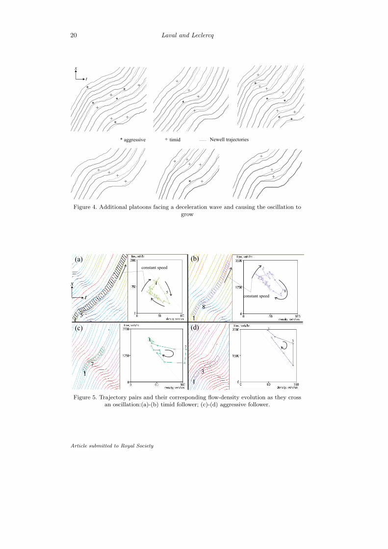
To study timid and aggressive driver behavior in more detail, figure 5 shows afew trajectory pairs and their corresponding flow-density evolution as they cross anoscillation. These have been computed using Edies’ generalized definitions (Edie,1961), which for an n-vehicle platoon inside an arbitrary time-space region A are:

k =n∑

i=1

Ti/|A|, q =n∑

i=1

Di/|A|, v = q/k =n∑

i=1

Di/n∑

i=1

Ti,

where the symbols k, q and v stand for density, flow and speed in A, respectively,|A| is the area of A, and Ti, Di are the ith vehicle travel time and distance traveledinside A, respectively.



Each small circle in the fundamental diagram on figure 5 corresponds to flow-density measurements inside a particular trapezoidal area in the correspondingtime-space diagram. The number “1” in each figure indicates the first such mea-surement; the rest of the measurements are consecutively added as the trajectorypair travels downstream. Parts a and b of the figure correspond to a timid follower,while parts c and d to an aggressive follower. One can see that

R-9: timid drivers seem to decelerate along the equilibrium branch (1 → 5 and 1→ 8 in parts a and b, respectively), and accelerate along a “lower” branch tocome back to the initial traffic state 1;

R-10: aggressive drivers decelerate along an “upper” branch (1 → 7 and 1 → 3 inparts c and d, respectively), and accelerate along the equilibrium branch tocome back to equilibrium;

R-11: shortly after the appearance of these non-equilibrium behaviors the speedof vehicles upstream rapidly drops to zero.

These remarks suggest that, unlike Newells conjectures, there appears to be multiplebranches on the fundamental diagram in congestion. At least one for equilibriumstates and two others for timid and aggressive driving behavior.

The vehicle speed decay towards zero along the oscillation can be seen in fig-ures 6 (US-101) and figure 7 (I-80). These figures present trajectories crossing fouroscillations at the time of their formation, and shows the speed of vehicles alongcharacteristics near deceleration waves. These characteristics are depicted as linesin each time-space diagram, and the speed of each vehicle was measured at the timethey cross this line. It can be seen that

R-12: vehicles speeds seem to decay from vehicle to vehicle according to a randomwalk with a negative drift;

R-13: this negative drift has an average of approximately -1.13 km/hr betweentwo consecutive vehicles and a standard deviation of 0.28 km/hr, both sitescombined, -1.25 km/hr and 0.29 km/hr at US-101, and -1 km/hr and 0.19km/hr at I-80. We can conclude that the drift at both sites appears to bedrawn from the same distribution.

R-14: from figure 6a,d and 7a,b,d there seems to be room for speculating that thefunctions depicted there are convex; i.e., speed drops faster at higher speeds.

Next, we propose a theory based on the above remarks. We will show that theexistence of non-equilibrium behavior alone is not enough to produce the kind ofoscillations seen in the data.

4. The continuous-time model

The model presented in this section is the continuous-time version of the modelin Laval and Leclercq (2008) extended to account for the remarks in the previoussection. In the spirit of the kinematic wave model (i) dynamics will be studiedalong characteristics traveling at −w, which is assumed constant; and (ii) vehiclepositions are obtained as the minimum of a free-flow term and a congestion term.



Our main assumption is that in congestion deceleration waves can trigger somedrivers initially in equilibrium to switch to two non-equilibrium “modes”, eithertimid or aggressive (R-4).

(a) The free-flow term

Following Laval and Daganzo (2006) we shall remove infinite accelerations inNewell’s model by incorporationg the vehicle kinematics model:

a(v) = am(1− v/u)− gG, (4.1)

with g = 9.81 m/s2. Eqn. (4.1) can be interpreted as the desired vehicle accelerationwhen traveling at a speed v on a freeway segments with a 100G% grade. Theparameter am gives the maximum acceleration, which is attained at v = 0; also,u/am can be interpreted as a relaxation time.

Here we note that (4.1) can be solved analyticaly to obtain vehicle displace-ments, xi+1(t), e.g. between t− τ and t:

xi+1(t) = vcτ − (1− e−bτ )(vc − vi+1(t− τ)), (4.2)

where vc = u(1 − gG/am) is the crawl speed and b = am/u. Then, the free-flowterm becomes:

xi+1(t) = xi+1(t− τ) + min{uτ, xi+1(t)}. (in free-flow) (4.3)

(b) The congestion term

In order to model non-equilibrium spacings in congestion, we use the dimension-less variable ηi+1(t) to denote the ratio between vehicle (i + 1)’s spacing, si+1(t),and its equilibrium spacing; i.e.:

si+1(t) = ηi+1(t)S(vi(t∗i )), (4.4)

where t∗i is the time when the characteristic reaching the follower at time t isemanated by the leader i (see figure 8a); i.e.:

t∗i = t− ηi+1(t)τ. (4.5)

This is true because S(v) is linear in both τ and δ, and therefore the non-equilibriumfundamental diagram ηi+1(t)S(vi(t

∗i )) can be interpreted as having wave trip time

ηi+1(t)τ and jam spacing ηi+1(t)δ. Therefore, vehicle trajectories in the proposedmodel can be obtained with the following generalization of (2.2):

xi+1(t) = xi(t∗i )− ηi+1(t)δ = xi (t− ηi+1(t)τ)− ηi+1(t)δ. (4.6)

As an illustration, consider figure 8a where the follower is in equilibrium at time t0and starts an aggressive behavior by driving faster than Newell’s trajectory. As inNewell’s model the trajectory of vehicle i can also be obtained in terms of the leadvehicle trajectory; i.e.:

xi+1(t) = x0

t− τi+1∑j=1

ηj(t∗j )

− δi+1∑j=1

ηj(t∗j ). (4.7)



Table 1. Dependence of the initial and target η values on the type of behavior and mode

timid aggressive

expansion contraction contraction expansion

η(0) 1 1 + α 1 1− α

ηT 1 + α 1 1− α 1

(c) The behavioral model

According to (R-7) and (R-8) we define two non-equilibrium “modes”:

• contraction mode: the driver seeks to shorten its spacing relative to be equi-librium spacing; i.e., the time derivative of η is negative, η′i+1(t) < 0;

• expansion mode: the diver seeks to widen its spacing relative to be equilibriumspacing; i.e., η′i+1(t) > 0.

It follows that, within this framework, a timid behavior is composed of an expansionfollowed by a contraction whereas an aggressive behavior is a contraction followedby an expansion. This is shown in figure 9, which depicts a leader introducing aspeed perturbation and the reaction of a timid (parts a and c) and an aggressive(parts b and d) driver as hypothesized here. The top row (bottom) of the figuredepicts a follower that completes his/her non-equilibrium cycle before (after) theperturbation is removed.

The transition between the two modes is modeled here using a single parameter,α, to represent the notion of a target deviation from equilibrium; i.e., a target valueof η, ηT ; see figure 9. Until this target is not achieved the driver remains in thecurrent mode. For simplicity in exposition, from now on t = 0 denotes the timewhen a driver switches from one mode to another. Both the initial value, η(0), atthe beginning of a mode and the target ηT depend on the type of behavior andmode, as shown in table 1.

It remains to establish how a driver goes from η(0) to ηT , i.e., the shape of η′(t).

Taking derivatives in (4.6), using S(vi(t∗i )) = τvi(t

∗i ) + δ and rearranging one finds

η′i+1(t) =vi(t

∗i )− vi+1(t)

S(vi(t∗i )). (4.8)

It follows that reasonable models for η′(t) should come from reasonable assumptionsregarding the speed difference between the two vehicles along characteristics vi(t

∗i )−

vi+1(t). Therefore, the proposed framework allows us to study a family of modelsthat generalize (2.3) by postulating

vi+1(t) = f(vi(t∗i )), (4.9)

where f(·) is an arbitrary function of the leader speed (and possibly some other ar-guments) that describes the follower’s behavior; see figure 8a. A potential practicallimitation of this approach is that for most specifications of f(·) the ODE (4.8)-(4.9) is nonlinear, and it may not be possible to solve it explicitly, or its solutionmight be non-algebraic. Fortunately, the specification

f(v) = v − εS(v), (4.10)



where the parameter ε has units of flow, accords well with remarks (R-12)-(R-14). To see this, Figure 8b presents the vehicle speeds predicted by (4.10) along acharacteristic (thick line) together with three random walks around it. Notice theslight convexity of the prediction line. Notably, (4.10) yields a linear solution for(4.8)-(4.9):

ηi+1(t) = ηi+1(0) + εt, (4.11)

where t = 0 denotes when the driver switches modes. Depending on the sign of εone can model expansions (ε > 0) or contractions (ε < 0).

(d) Some properties for the lead vehicle problem

We shall analyze here the analytical solution of the proposed model for a leadvehicle that decelerates instantaneously to a speed v0 followed by a platoon incongestion. This platoon is assumed homogeneous (all drivers timid or aggressive)and in a stationary initial (non-)equilibrium state characterized by η(0) = η0; oncethe leader i = 0 decelerates at (t, x) = (0, 0) all drivers seek a common target ηTand stay at this target once it is reached.

Figure 10a shows the (exact) solution for a platoon of seven timid vehicles.Accordingly to Table 1 and Figure 9a, the expansion mode is implemented such thatat t=0 (when the leader reduces its speed to v0) ε > 0 is set until η = ηT = 1+α isreached. The case of an aggressive platoon is shown in figure 10b. In this case, thecontraction mode implies that at t=0, ε < 0 is set until η = ηT = 1− α is reached.

(i) Speeds in contraction and expansion modes

One can obtain the speeds v1, v2, . . . , v7 in figure 10 by noting that they aretime-independent (since the speed of the first vehicle is constant) and “unfolding”the iterative relationship (4.9)-(4.10): vi+1 = (1− ετ)vi− εδ. We find that for t ≥ 0the speed of vehicle i is given by

vi = (v0 + w) (1− ετ)i − w. (4.12)

Of course, we also require 0 ≤ vi ≤ u. Noting that |ε|S(v) ≈1 km/hr from figures6, 7 and 8b it follows that |ε|τ should be in the order of 10−2. Therefore, for fixed|ε| the magnitude of the speed change along the platoon are almost identical forexpansions (ε > 0) and contractions (ε < 0). Eqn. (4.12) can be solved for i toobtain the number of vehicles upstream of the leader that it takes to reach a givenspeed v:

i(v) = log

(v + w

v0 + w

)/ log (1− ετ) , (4.13)

which should be comparable with (v0 − v)/(v0 + w)/ετ if |v0 − v| is not too big.

(ii) Iso-η contours

Notice that in our model the value of η is not constant along characteristics. Tosee this, note that in our example ηi(t) = η0 + ε(t− iη0τ) and xi(t) = −iδη0 + (t−iη0τ)vi, where vi is given by (4.12). Eliminating i in these two equations yields theiso-η contours η = c; i.e.:

x(t) = c(v0 + w)(1− ετ)t−cη0τ − tw, (iso-η contours) (4.14)



where c = (c − η0)/ε. This indicates that for expansions (ε > 0) the first term inthe RHS tends to 0 as t → ∞ so that all iso-η contours tend to the line x = −wtfrom above; in contractions this term tends to ∞ as t → ∞ and all iso-η contourstend to be vertical as time passes. This can be verified in figure 10. In fact, it canbe seen in part a that the iso-η contours for timid drivers always travel faster than−w, with the the iso-ηT contour being the fastest (as shown by the bold curve infigure). The first vehicle to reach ηT is i = 1 at point “1” in the figure, where awave is emanated. Once vehicles cross the iso-ηT contour their trajectory is givenby Newell’s model in the sense that vehicle speeds along the characteristics areconstant. This produces the narrow bands shown in the figure which result in apiece-wise linear acceleration fan.

Figure 10b shows that in the case of aggressive drivers, the iso-η contours travelat a speed lower than −w, which gradually decreases with c. The first vehicle toreach ηT is i = 1 at point “2” in the figure. From this point on its speed changes tov0 and a wave is emanated upstream traveling at −w. When this wave crosses eachvehicle in the platoon, they decelerate gradually since they are still in contractionmode. They reach their target ηT at the bold line in the figure, which happensto be flat in this particular example but can even travel downstream, bearing astriking resemblance with the precursor region described in figure 3. This regioncan be described as a deceleration fan.

(e) Flow-density paths

The path in the flow-density diagram for a given trajectory pair, where theleader’s speed is v(t), can be obtained in parametric form by {k(t) = 1/(η(t)S(v(t))),q(t) = v(t)k(t)} which is valid only in 1− α ≤ η(t) ≤ 1 + α. In the case of a leaderadvancing at constant acceleration, v(t) = v0 + at, eliminating t in the above para-metric equations gives

q(k) =

√(a

ε(κw − η0(v0 + w)k) +

1

4(a

εη0 + v0 + w)2k

)k − 1

2(a

εη0 − v0 + w)k,

(4.15)which is now valid only in w(κ/(1+α)−k) ≤ q(k) ≤ w(κ/(1−α)−k). Notice thatq(k) = v0k when a = 0; i.e., contractions and expansions are performed along linesof constant speed when the leader does not accelerate. This can be seen in the dataof figure 5a-b.

Interestingly, the leader’s acceleration and the model parameter ε always appearin (4.15) as a ratio, a/ε. This implies that the situations ε ≥ 0, a ≥ 0 and ε ≤ 0, a ≤0 are described by the same family of flow-density trajectories; so are ε ≤ 0, a ≥ 0and ε ≥ 0, a ≤ 0. Six such families are shown in figure 11. In each flow-densitydiagram in figure the value of a/ε is fixed and (4.15) is evaluated for six differentvalues of v0; this process is shown in parts a and d of the figure for a single valueof v0.

One can obtain flow-density trajectories similar to the ones in figure 5 by care-fully combining different branches from different parts in figures 11. For example,the timid behavior in figure 5a can be seen–at least qualitatively–combining path1 → 2 in figure 11c, 2 → 3 in part f and 3 → 1 in part c. The aggressive behaviorof figure 5c can be described within single-family as shown by the path depicted in



figure 11e. Notice that for maximum analogy with figure 5c, for this path we haveassumed that the jam density cannot be surpassed. However, this restriction doesnot change the macroscopic behavior of the model significantly.

It is worth noting that the proposed model does not specify a behavioral modelwhen the leader accelerates (a > 0), provided that the leader has decelerated pre-viously and thus triggered non-equilibrium behavior upstream.

Next, we resort to the numerical resolution of the proposed theory to showthat uphill grades may produce perturbations that trigger the formation of trafficoscillations with regular periods.

5. The discrete model

In order to perform numerical simulations we resort to the discrete model proposedin Laval and Leclercq (2008), which turns out to be a discretization of a specialcase of the continuous-time framework proposed here.

Let the superscript j denote the value of a variable at discrete time tj = jτ, j =

0, 1, 2 . . ., e.g. xji = xi(tj). Here we use:

xj+1i+1 = min{xj

i+1 +min{uτ, xj+1i+1}︸︷︷︸

free-flow term

, xji + τvj+1

i − ηj+1i+1S(v

j+1i )︸︷︷︸

congestion term

}. (5.1)

The free-flow term is exact as it corresponds to (4.3). The congestion term corre-sponds to an “Euler-type” discretization in that it gives the exact solution of ourcontinuous-time model assuming that during tj < t ≤ tj+1 both vi(t) and ηi(t) are

constant and equal to vj+1i and ηj+1

i , respectively; see Laval and Leclercq (2008).

Notice how model (5.1) gives Newell’s model (2.2) when a = ∞ and ηj+1i+1 = 1, as

expected. The update of η is now:

ηj+1i+1 = ηji+1 + ετ, (deterministic) (5.2)

as suggested by (4.11). Two other models will be tested here:

ηj+1i+1 = ηji+1 + ετ +N(0, σ2τ), (random walk) (5.3)

and

ηj+1i+1 = ηji+1 +N(0, σ2τ), (fully stochastic) (5.4)

where N(0, σ2τ) denotes a normal random variable with zero mean and varianceσ2τ . In all models we impose 1− α ≤ ηj+1

i+1 ≤ 1 + α.

Model (5.3) was suggested by (R-12) as it implies that ηj+1i+1 is a Brownian motion

(or a random walk with normally distributed steps). This specification allows usto “generalize” (4.10), which was chosen for mathematical convenience–althoughjustified by figures 6 and 7–rather than driving behavior considerations. Model(5.4) is “fully stochastic” as described in the introduction; i.e., at each time stepdrivers randomly select to increase or decrease their speed independently of thelogic proposed in this paper. Recalling (4.8) speed differences vi(t

∗i ) − vi+1(t) in

this model will be approximately N(0, (S(vi(t∗i ))σ)

2/τ).



6. Periodic oscillations at uphill segments

In this section we study a level 1-lane road with an uphill segment of length L =300m and a 100G% grade. The desired acceleration of all vehicles is given by (4.1)and the proportion of timid and aggressive drivers is rT and rA, respectively; theremaining proportion 1 − rT − rA obeys Newell’s model. The system is empty att = 0, when vehicles enter the upstream boundary of the segment in equilibrium(ηi = 1) and at capacity (traffic state “1” in figure 2a). Vehicles exit the system atthe downstream boundary located 500 m downstream of the top of the uphill.

The three models in the previous section were run for all combinations of vari-ables G, am, rA, rT and parameters ε, α, σ, each one varying within a range observedto produce noticeable qualitative changes. The length of the segment is 3 km, theupgrade is located at x =2 km and its length is fixed at L = 300m. The simulationtime is one hour in all cases, and the fundamental diagram parameters are: u = 120km/hr, w = 20 km/hr and κ = 150 veh/km.

Figure 12 shows typical speed maps from the deterministic model; left panelsonly consider timid drivers whereas right panels only aggressive. It can be seen howdifferent oscillation periods can be obtained varying the model parameters. Noticethe precursor regions in part a of the figure, similar to the ones observed in figures 1and 3. It was verified that the experiments with only aggressive drivers produceoutputs similar to the left panels but also the more complex patterns on the right.In particular, notice in part b how certain waves seem to merge with adjacent onesor simply dissipate, while only a few “survive” and propagate upstream unchanged.

Figure 13 shows typical speed maps obtained with the random walk in partsa,b and fully stochastic models in c,d. Parts a,b can be compared with parts a,bin figure 12, which shows, at least qualitatively, that these two models exhibit thesame properties; this was verified for a wide range of parameter values. Parts c,d offigure 13 show that the fully stochastic model is able to produce periodic oscillations(part c) but also exhibits rather questionable patterns (part d).

To quantify the main differences of the models, the oscillation period and am-plitude of the oscillations were analyzed over a 1-hr speed time-series at locationx = 1km for all runs (approximately 2000 per model). We used the method pro-posed in Li et al. (2009), which uses Fourier’s spectrum analysis to minimize thebias in estimating amplitudes and periods of traffic time-series data. Figure 14shows the oscillation period and amplitude against the dimensionless ratio gG/am,for all three models. The different data points were obtained with different valuesof the parameter α and averaged across all remaining parameters. This parameteris common to all models and is a measure of driver behavior variability.

Regarding the period we observe that: (i) for all models there is a well-defineddecreasing relationship with gG/am, (ii) in the range 0.4 ≤ gG/am ≤ 0.8 all mod-els produced a very similar period in the range 3-10 minutes, (iii) in the rangegG/am ≤ 0.4 the deterministic and random walk model predict significantly higheroscillation periods than the fully stochastic model, and (iv) aggressive driver be-havior systematically implies longer periods. Similarly, for the amplitude we notethat: (v) the deterministic and random walk model predict a well-defined decreas-ing relationship with gG/am, whereas the fully stochastic model predicts a concaverelationship, (vi) for all values of gG/am the fully stochastic model results and



significantly lower amplitude values, (vii) aggressive driver behavior systematicallyimplies larger amplitudes.

7. Discussion

We have introduced a framework based on empirical observation, which predicts thespeed decay inside traffic oscillations produced by small perturbations on a singlelane absent of lane-changes. This initial perturbation may have many causes, andthis paper showed that upgrade sections is one of them. Moreover, the proposedtheory seems to capture the mechanism that triggers periodic oscillations in thistype of bottleneck.

The empirical evidence presented here seems to contradict existing conjectures.We found no evidence that oscillations growth is caused by drivers seeking lane-changing opportunities, as suggested in Kerner (2004). Nor did we find evidencesupporting Newell’s acceleration and deceleration branches. We believe it seemsmore appropriate to talk about aggressive and timid branches, which act more likereflecting bounds for the flow-density paths described here.

The iso-η contours η = ηT are significant because in real data they would appearto be waves traveling at nearly constant speeds, but this constant speed can be verydifferent in each realization; see figure 10. This may be an explanation for the shapeof iso-speed contours in the precursor periods of figures 3b,c.

Our simulation results indicate that fully stochastic models exhibits questionablebehavior. To verify this assertion, we have analyzed the loop detector data locatedjust upstream of the bottom of the 5.6% uphill segment in US-101 alluded to insection 3. This steep grade should correspond to gG/am-values of about 0.7. Thespeed time-series during the morning rush exhibits a period of about 7 min with anamplitude of about 15 km/hr. The reader can verify this data point accords verywell with all models but the fully stochastic one.

The simulation experiment also revealed that the deterministic and random walkmodel are essentially identical, at least with respect to the type of oscillations theyproduce. Therefore, there may be numerous variations of the basic deterministicmodel presented here that would produce similar results. We conclude that oscil-lations are a consequence of driver heterogeneous reactions to deceleration wavesas postulated here, but independently of the details of this behavior. Notice theanalogy to Wilson’s finding (Wilson, 2008) mentioned in the introduction.

The physical explanation of the correlation between the model parameters andvariables and oscillation characteristics is not included here for brevity, but is thesubject of current research by the authors. Suffice it to say that in the case offigures 12a,e the oscillation period, or the time until the next oscillation, is a directconsequence of the discharge flow from the previous oscillation and of the speed ofthose vehicles when approaching the bottom of the uphill. This is true because adeceleration wave is felt whenever the speed of incoming vehicles is greater than thespeed on the upgrade (which is likely to be close to the crawl speed u(1−gG/am)).And the probability of an oscillation to form increases with the incoming flow,which in turn increases as the oscillation propagates upstream; see the “lower flow”and “higher flow” zones in figure 12e. Consideration shows that these two factorsmay explain the high correlation between the period and the dimensionless ratiogG/am: the steeper the upgrade the lower the crawl speed, the faster vehicles inside



the oscillation will reach a full stop, and the faster these vehicles will be able toaccelerate back to the crawl speed.

Finally, the proposed mechanism can also explain the hysteresis phenomenon(Treiterer and Myers, 1974). Accordingly, hysteresis happens whenever a driverreaches equilibrium after the disturbance has passed, as in figure 9c,d. In both cases,flow-density measurements before and after the deceleration wave would appear indifferent branches of the fundamental diagram. However, these branches are notrelated to vehicles accelerations or decelerations as previously thought (Treitererand Myers, 1974), but rather to aggressive and timid behaviors. In fact, as shownin figure 11c,f, the acceleration path of an aggressive driver is above its decelerationpath, which contradicts Treiterer and Myers (1974).

Acknowledgment. This research was partially supported by the Georgia De-partment of Transportation project 2006N78, and the National Science Foundationaward number 0856218. The authors would like to thank two anonymous refereesand D. Chen, B. Chilukuri, H. Zhengbing, X. Li and Y. Ouyang, whose commentsand suggestions greatly improved the quality of this paper.

References

Ahn, S., 2005. Growth of oscillations in queued traffic. Ph.D. thesis, Dept. of CivilEngineering, Univ. of California, Berkeley.

Ahn, S., Cassidy, M., 2006. Freeway traffic oscillations and vehicle lane-changemanoeuvres. In: Heydecker, B., Bell, M., Allsop, R. (Eds.), Forthcoming in 17thInternational Symposium on Transportation and Traffic Theory. Elsevier, NewYork.

Ahn, S., Cassidy, M., Laval, J. A., 2004. Verification of a simplified car-followingtheory. Transportation Research Part B 38 (5), 431–440.

Barlovic, R., Huisinga, T., Schadschneider, A., Schreckenberg, M., 2002. Openboudaries in a cellular automaton model for traffic flow with mtastable states.Physical Review E (66), 1–11.

Barlovic, R., Santen, L., Schadschneider, A., Schreckenberg, M., 1998. Metastablestates in cellular automata for traffic flow. The European Physical Journal B (5),793–800.

Cassidy, M., Windover, J., 1995. Methodology for assessing dynamics of freewaytraffic flow. Transportation Research Record (1484), 73–79.

Chevallier, E., Leclercq, L., 2009. Do microscopic merging models reproduce theobserved priority sharing ratio in congestion? Transportation Research Part C17 (3), 328–336.

Chiabaut, N., Buisson, C., Leclercq, L., 2009a. Fundamental diagram estimationthrough passing rate measurements in congestion. IEEE transactions on Intelli-gent Transportation Systems 10 (2), 355–359.

Chiabaut, N., Leclercq, L., Buisson, C., 2009b. From heterogeneous drivers tomacroscopic patterns in congestion. Transportation Research Part B, 44(2), 2010,299-308.



Daganzo, C. F., 2005. A variational formulation of kinematic waves: Basic theoryand complex boundary conditions. Transportation Research Part B 39 (2), 187–196.

Del Castillo, J. M., 2001. Propagation of perturbations in dense traffic flow: a modeland its implications. Transportation Research Part B 35 (2), 367–390.

Edie, L. C., 1961. Car following and steady-state theory for non-congested traffic.Operations Research 9, 66–77.

Foster, J., 1962. An investigation of the hydrodynamic model for traffic flow withparticular reference to the effect o various speed-density relationships. In: 1stConference of the Australian Road Research Board. p. 229257.

Helbing, D., Hennecke, A., Shvetsov, V., Treiber, M., 2001. Master: Macroscopictraffic simuation based on a gas-kinetic, non-local traffic model. TransportationResearch Part B 35 (2), 183–211.

Helbing, D., Treiber, M., 1998. Gas-kinetic-based traffic model explaining observedhysteresis phase transition. Physical Review Letters 81 (14), 3042–3045.

Igarashi, Y., Itoh, K., Nakanishi, K., Ogura, K., Yokokawa, K., 2001. Bifurcationphenomena in the optimal velocity model for traffic flow. Physics Reviews E64 (4), 47102.

Kerner, B. S., 2004. The physics of traffic. Springer.

Kerner, B. S., Rehborn, H., 1996. Experimental features and characteristics of trafficjams. Physics Reviews 53 (E), R1297–R1300.

Khoshyaran, M., Lebacque, P., 2007. A stochastic macroscopic traffic model devoidof diffusion. In: Appert-Rolland, C., Lassarr, S., Gondret, P., Dauchot, O., Sykes,C. (Eds.), Traffic and Granular Flow ’07. Springer Berlin Heidelberg, pp. 139–150.

Kim, T., Zhang, H. M., 2008. A stochastic wave propagation model. TransportationResearch Part B 42 (7-8), 619–634.

Kometani, E., Sasaki, T., 1958. On the stability of traffic flow. J. Operations Re-search Japan (2), 11–26.

Koshi, M., Kuwahara, M., Akahane, H., 1992. Capacity of sags and tunnels injapanese motorways. ITE Journal (May issue), 17–22.

Laval, J. A., 2005. Linking synchronized flow and kinematic wave theory. In: Schad-schneider, A.and Poschel, T., Kuhne, R., Schreckenberg, M., Wolf, D. (Eds.),Traffic and Granular Flow ’05. Springer, pp. 521–526.

Laval, J. A., 2006. Stochastic processes of moving bottlenecks: Approximate formu-las for highway capacity. Transportation Research Record 1988, 86–91.

Laval, J. A., Chen, D., Ben Amer, K., Guin, A., Ahn, S., 2009. Evolution of oscilla-tions in congested traffic: Improved estimation method and additional empiricalevidences. Transportation Research Record 2124, 194–202.



Laval, J. A., Daganzo, C. F., 2006. Lane-changing in traffic streams. TransportationResearch Part B 40 (3), 251–264.

Laval, J. A., Leclercq, L., 2008. Microscopic modeling of the relaxation phenomenonusing a macroscopic lane-changing model. Transportation Research Part B 42 (6),511–522.URL http://dx.doi.org/10.1016/j.trb.2007.10.004

Leclercq, L., Chiabaut, N., Laval, J., Buisson, C., 2007. Relaxation phenomenonafter changing lanes: Experimental validation with NGSIM data set. Transporta-tion Research Record 1999, 79–85.

Li, X., Peng, F., Ouyang, Y., 2009. Measurement and estimation of traffic oscillationproperties (in press). Transportation Research Part B.

Lighthill, M. J., Whitham, G., 1955. On kinematic waves. I Flow movement in longrivers. II A theory of traffic flow on long crowded roads. Proceedings of the RoyalSociety of London 229 (A), 281–345.

Mauch, M., Cassidy, M. J., 2002. Freeway traffic oscillations: Observations andpredictions. In: Taylor, M. (Ed.), 15th Int. Symp. on Transportation and TrafficTheory. Pergamon-Elsevier, Oxford,U.K.

Munoz, J., Daganzo, C. F., 2000. Experimental characterization of multi-lane free-way traffic upstream of an off-ramp bottleneck. Tech. Rep. UCB-ITS-PWP-2000-13, Inst. Trans. Studies, Univ. of California, Berkeley, CA.

Nagel, K., Schreckenberg, M., 1992. A cellular automaton model for freeway traffic.Journal of Physics I (2), 2221 – 2229.

Newell, G. F., 1961. Non-linear effects in the dynamics of car following. Opns. Res.2 (9), 209–229.

Newell, G. F., 1962. Theories of instability in dense highway traffic. J. OperationsResearch Japan 1 (5), 9–54.

Newell, G. F., 1965. Instability in dense highway traffic: A review. In: Almond,J. (Ed.), 2nd. International Symposium on the Theory of Road Traffic Flow.London, pp. 73–83.

Newell, G. F., 2002. A simplified car-following theory : a lower order model. Trans-portation Research Part B 36 (3), 195–205.

Ngoduy, D., 2008. Operational effect of acceleration lane on main traffic flow atdisconituities. Transportmetrica 4 (3), 195–207.

Ngoduy, D., Hoogendoorn, S., Van Zuylen, H., 2006. New continuum traffic modelfor freeway with on- and off-ramp to explain different traffic congested states.Transportation Research Record (1962), 92–102.

Orosz, G., Wilson, R. E., Szalai, R., Stepan, G., 2009. Exciting traffic jams: Non-linear phenomena behind traffic jam formation on highways. Physics Reviews E80 (4), 46205.



NGSIM, 2006. Next generation simulation.URL http://ngsim.fhwa.dot.gov/

Richards, P. I., 1956. Shockwaves on the highway. Operations Research (4), 42–51.

Shvetsov, V., Helbing, D., 1999. Macroscopic dynamics of multilane traffic. PhysicalReview E 59 (6), 6328–6339.

Treiterer, J., Myers, J. A., 1974. The hysteresis phenomenon in traffic flow. In:Buckley, D. J. (Ed.), 6th Int. Symp. on Transportation and Traffic Theory. A.H.and A.W. Reed, London,, pp. 13–38.

Wilson, R. E., 2008. Mechanisms for spatio-temporal pattern formation in highwaytraffic models. Phil. Trans. R. Soc. A 366 (1872), 2017–2032.

Yeo, H., Skabardonis, A., 2009. Understanding stop-and-go traffic in view of asym-metric traffic theory. In: Lam, W., Wong, S. C., Lo, H. (Eds.), 18th InternationalSymposium of Traffic Theory and Transportation. pp. 99–116.

0

200

400

600

7:50 7:53 7:56 7:59 8:02 8:05

8:05 8:08 8:11 8:14 8:17 8:20

8:20 8:23 8:26 8:29 8:32 8:35

time, min

0

200

400

600

time, min

0

200

400

600

time, min1 2 3 4% grade

1 2 3 4% grade

1 2 3 4% grade

lane-changes

-w > -16 km/hr

dis

tance

, m

dis

tance

, m

dis

tance

, m

Figure 1. NGSIM trajectories for the median lane in the vicinity of Lankershim Av onUS-101 freeway in Los Angeles, California. Also shown is the percentage grade as a functionof distance.



(a)

kdensity

flo

w

u -w

1

speed

spac

ing

d=1/k

t k= 1/w

u

S v v( ) = d + t t

x

t

d

S v t( ( ))i

New

ell t

raje

ct

ory

vi+ i1( ) ( )t+ = v tt

-w

v ti( )

v ti( )t

shift

(b)

(c)

2

Figure 2. Newell’s car-following model: (a) triangular flow-density diagram with parame-ters: free-flow speed u, wave speed −w, and jam density κ; (b) solution of Newell’s modelin congestion: vehicle (i + 1)’s trajectory is that of its leader i but shifted τ time unitsforward in time and δ distance units upstream in space; (c) spacing-speed relationshipcorresponding to the decreasing branch of the triangular flow-density diagram.



dis

tance

,640 m

time, 15 min

precursor period

t

x

aggressivetimid

*+

*

*

*

+

+

+

*+

*

+

Newell’s trajectory

precursor period

(a)

(b) (c)

(d) (e)

zoom-in zoom-in

15 km/hr

28 km/hr

35 km/hr

Figure 3. A more detailed view of the first 15 minutes of the data



aggressive

*

*

*

*

*

+

+

*

*

*+

+t

x

*

*

+

+

+

+++

++

+

+

+

Newell trajectoriestimid

+

+

+

+

++

+

+

+

*

*

*

+

+

+

+

Figure 4. Additional platoons facing a deceleration wave and causing the oscillation togrow

1

(a) (b)

(c) (d)

t

x 11

8

85

5

7

7

3

3

constant speed

1

constant speed

1

1

1

Figure 5. Trajectory pairs and their corresponding flow-density evolution as they crossan oscillation:(a)-(b) timid follower; (c)-(d) aggressive follower.



~ -1 km/hr

-1.4

-1.6

-1.2

-0.8

t

x

(a) (b)

(c) (d)

Figure 6. Trajectories crossing four oscillations on US-101 at the time of their formationand speed of vehicles along characteristics near deceleration waves.

t

x

-1

-1.3

-0.9

-0.8

(a) (b)

(c) (d)

Figure 7. Same as figure 6 but for I-80.



-w

t

x

td

hthd

hS v t*( ( ))i i

Newell trajectory

vi+ i i1( ) ( ( ))t =f v t*

-w

v t*i 0( )

t0 t

v t*i i( )

spee

d, km

/hr

v

veh #, i

0 5 10 15 20

5

10

15

20

randomwalks

(b)(a)

slope ( )= - S ve

Figure 8. (a) Time space diagram of a pair of trajectories in the proposed model; (b)vehicle speed decays toward zero along the oscillation predicted by (4.10) using ε = 100veh/hr.

expantion contraction

-w

vb

h = (1+a)T S v( )b

va

va expantioncontraction

-w

vb

va

va

(a) (b)

t

x

Newell’s trajectory

h = 1

h < 1

h = 1h‘ 0< h‘ 0>h = 1

h > 1

h = 1h‘ 0> h‘ 0<

expantion

con

trac

tio

n

-w -w

expan

tion

contraction

(c) (d)

h = (1-a)T S v( )b

h = (1+a)T S v( )a

h = (1-a)T S v( )a

va v

a

va v

a

vb v

b

e = 0 e = 0e > 0 e < 0 e = 0 e = 0e < 0 e > 0

Figure 9. Time space-diagrams of a leader introducing a speed perturbation and the re-action of a timid (a,c) and an aggressive (b,d) driver proposed here. Top (bottom) row:drivers complete their non-equilibrium cycle before (after) the perturbation has passed.



(b)

-w

v0

-w

v2

h=h

0

h=hT

v0

v4

v6

v=v1

v=v

5

piece-wise

linea

r

(a)

-w

-w

v0

v2

v0

v4

v6

t

x

h=h0

h=hT

iso-h

iso-hacceleratio

n fan

dece

lera

tion fa

n2

v=v

3

0t

x

0

1

Figure 10. Exact solution for a platoon of seven (a) timid and (b) aggressive drivers.Following Table 1 and Figure 9, the expansion for timid drivers is implemented such thatat t=0 (when the leader reduces its speed to v0) ε > 0 is set until η = ηT = 1 + α isreached; for the contraction of aggressive drivers, at t=0, ε < 0 is set until η = ηT = 1−αis reached. It was assumed α = 0.6, |ε| = 200 veh/hr.

expan

sion +

lea

der

acc

eler

ates

or

contr

acti

on +

lea

der

dec

eler

ates

contr

acti

on

expan

sion +

lea

der

dec

eler

ates

+ l

eader

acc

eler

ates

or

k

q-20

k

q-40

k

q-100

k

q20

k

q40

k

q100

v0

(k/(1+a)-)

q(k)=w

k

(k/(1-a)-)

q(k)=w

k

h=1-a

h=1+a

4

jam densitycap

1

2

23

3

v0

-w

(a) (b) (c)

(d) (f)(e)

Figure 11. Families of flow-density trajectories for different values of a/ε; (4.15) is evaluatedfor v0 = {0, 10, 20, 30, 40, 60, 90}. Notice how timid behavior in figure 5a can be obtainedby combining path 1 → 2 in (c), 2 → 3 in (f) and 3 → 1 in (c); the aggressive behavior offigure 5c can be described within (e).



e

a

= 75 veh/hr

= 0.2

= 1 m/s

= 0.6

a

r

m

T

2

G

r

= 5%

= 0A

e = 200 veh/hr

= 5%

= 0

= 0.2

= 1 m/s

= 0.9

a

a

r

m

T

2

G

rA

grade

(a) (b)

(c) (d)

spac

e, 3

km

time, 60 min

spac

e, 5

km

time, 80 min

e

a

= 200 veh/hr

= 0.4

= 0.6 m/s

= 0

a

r

m

T

2

G

r

= 4%

= 0.3A

e = 200 veh/hr

= 5%

= 0.9

= 0.2

= 0.6 m/s

= 0

a

a

r

m

T

2

G

rA

spac

e, 5

km

time, 80 min

spac

e, 3

km

time, 60 min

(e) (f)

spac

e,500 m

time, 3 min

spac

e, 8

00 m

time, 4 min

only timid drivers only aggressive drivers

bottom ofupgrade

bottom ofupgrade

higher flow

Figure 12. Typical speed maps obtained with the deterministic model.

s

a

= 20 hr

= 0.35

= 1 m/s

= 0.05

-1

a

r

m

2

G = 5%

(c)

s = 20 hr-1

= 0.35

= 0.6 m/s

= 0.2= 3%

a

a

r

G

m

2

(d)

spac

e, 3

km

time, 60 min

spac

e, 3

km

time, 60 min

fully stochastic model

s = e = 75 hr-1

;other parameters as in figure 11a

grade

(a) (b)

spac

e, 3

km

time, 60 min

spac

e, 5

km

time, 80 min

random walk

s = e = 200 hr-1

;other parameters as in figure 11a

Figure 13. Typical speed maps obtained with the (a,b) random walk and (c,d) fullystochastic models.



0

5

10

15

20

0.2 0.4 0.6 0.8

0

5

10

15

0.2 0.4 0.6 0.8

a = 0.2

a = 0.3

a = 0.4

Aggressive

0

10

20

30

0.2 0.4 0.6 0.8

a = 0.2

a = 0.3

a = 0.4

Timid

0

20

40

60

0.2 0.4 0.6 0.8gG/am

per

iod, m

in

ampli

tude,

km

/hr

gG/am

gG/am

per

iod, m

in

ampli

tude,

km

/hr

gG/am

gG/am

per

iod, m

in

ampli

tude,

km

/hr

gG/am

0

5

10

0.2 0.4 0.6 0.8

a = 0.5 a = 1.5 a = 2.5 a = 3.5

0

5

10

0.2 0.4 0.6 0.8

a = 0.2

a = 0.3

a = 0.4

Aggressive

a = 0.2

a = 0.3

a = 0.4

Timid

mean

(deterministic)

(random walk)

(fully stochastic)

(a)

(b)

(c)

Figure 14. Oscillations period against the dimensionless ratio gG/am. (a) deterministic,(b) random walk and (c) fully stochastic models.


Documents

A mechanism to describe the formation and propagation of stop-and-go waves in congested freeway traffic