Capacity Modeling of Freeway Weaving Sections

by Yihua Zhang

Dissertation submitted to the Faculty of

Virginia Polytechnic Institute and State University

in partial fulfillment of the requirement for the degree of

Doctor of Philosophy

in

Civil Engineering

Dr. Hesham Rakha, Chair

Dr. Ihab El-Shawarby, Committee Member

Dr. Pushkin Kachroo, Committee Member

Dr. Dusan Teodorovic, Committee Member

Dr. Samuel Tignor, Committee Member

May, 2005

Blacksburg, Virginia

Keywords: Modeling of Weaving Sections, Highway Capacity Manual, INTEGRATION

Software, Traffic Modeling, and Freeway Capacity Analysis

Copyright 2005, Yihua Zhang

Capacity Modeling of Freeway Weaving Sections

Yihua Zhang

Abstract The dissertation develops analytical models that estimate the capacity of freeway weaving sections. The analytical models are developed using simulated data that were compiled using the INTEGRATION software. Consequently, the first step of the research effort is to validate the INTEGRATION lane-changing modeling procedures and the capacity estimates that are derived from the model against field observations. The INTEGRATION software is validated against field data gathered by the University of California at Berkeley by comparing the lateral and longitudinal distribution of simulated and field observed traffic volumes categorized by O-D pair on nine weaving sections in the Los Angeles area. The results demonstrate a high degree of consistency between simulated and field observed traffic volumes within the various weaving sections. Subsequently, the second validation effort compares the capacity estimates of the INTEGRATION software to field observations from four weaving sections operating at capacity on the Queen Elizabeth Way (QEW) in Toronto, Canada. Again, the results demonstrate that the capacity estimates of the INTEGRATION software are consistent with the field observations both in terms of absolute values and temporal variability across different days. The error was found to be in the range of 10% between simulated and field observed capacities.

Prior to developing the analytical models, the dissertation presents a systematic analysis of the factors that impact the capacity of freeway weaving sections, which were found to include the length of the weaving section, the weaving ratio (a new parameter that is developed as part of this research effort), the percentage of heavy vehicles, and the speed limit differential between freeway and on- and off-ramps. The study demonstrates that the weaving ratio, which is currently defined as the ratio of the lowest weaving volume to the total weaving volume in the 2000 Highway Capacity Manual, has a significant impact on the capacity of weaving sections. The study also demonstrates that the weaving ratio is an asymmetric function and thus should reflect the source of the weaving volume. Consequently, a new definition for the weaving ratio is introduced that explicitly identifies the source of the weaving volume. In addition, the study demonstrates that the length of the weaving section has a larger impact on the capacity of weaving sections for short lengths and high traffic demands. Furthermore, the study demonstrates that there does not exist enough evidence to conclude that the speed limit differential between mainline freeway and on- and off-ramps has a significant impact on weaving section capacities. Finally, the study demonstrates that the HCM procedures model the heavy duty vehicle impacts reasonably well.

This dissertation presents the development of new capacity models for freeway weaving sections. In these models, a new definition of the weaving ratio that explicitly accounts for the source of weaving volume is introduced. The proposed analytical models estimate the capacity of weaving sections to within 12% of the simulated data, while the HCM procedures exhibit errors in the range of 114%. Among the newly developed models, the Artificial Neural Network (ANN) models performs slightly better that the statistical models in terms of model prediction errors. However, the sensitivity analysis results demonstrate unrealistic behavior of the ANN models

iii

under certain conditions. Consequently, the use of a statistical model is recommended because it provides a high level of accuracy while providing accurate model responses to changes in model input parameters (good response to the gradient of the input parameters).

iv

Acknowledgements

I would like to express my sincere gratitude to Dr. Hesham Rakha, for serving as my advisor and helping me through the development of this dissertation during the past years. I am very much thankful to him for the guidance and the encouragement he provided during my studies at Virginia Tech. I would also like to express my sincere thanks to all my other committee members: Dr. Ihab El-Shawarby, Dr. Pushkin Kachroo, Dr. Dusan Teodorovic, and Dr. Samuel Tignor. They have given me a lot of very good advice for my study, and they are very supportive whenever I need help. Special thanks go to my wife, Xiaoli. She has sacrificed much. I thank her for her support and understanding. Here I also thank my big family in China: my parents, my brother and my sister. Although they are more than 10 thousand kilometers away from me, their endless love for me always encourages me to make progress. I am also very grateful to my passed grandpa and grandma. Their love for me has been engraved in my heart and will encourage me forever. And finally, to all my friends at Virginia Tech, who made my stay most memorable and enjoyable, goes sincere thanks.

v

Table of Contents

Abstract .......................................................................................................................................... iii Acknowledgements........................................................................................................................ iv Table of Contents............................................................................................................................ v List of Tables ................................................................................................................................ vii List of Figures .............................................................................................................................. viii Chapter 1. Introduction ................................................................................................................... 1

1.1 Problem Overview ............................................................................................................ 1 1.2 Research Objectives.......................................................................................................... 2 1.3 Research Contributions..................................................................................................... 3 1.4 Dissertation Layout........................................................................................................... 3

Chapter 2. Literature Review.......................................................................................................... 5 2.1 1950 HCM procedures...................................................................................................... 5 2.2 Drew (1968) ...................................................................................................................... 5 2.3 PINY (1976)...................................................................................................................... 6 2.4 Leish’s procedure (1981) .................................................................................................. 7 2.5 JHK (1984)........................................................................................................................ 9 2.6 1985 HCM procedures...................................................................................................... 9 2.7 Fazio and Rouphail (1986).............................................................................................. 11 2.8 Cal. Berkeley (1989, 1991, 1993)................................................................................... 11 2.9 Fazio and Rouphail (1990, 1993).................................................................................... 16 2.10 Wang, Cassidy, Chan, and May (1993) ........................................................................ 18 2.11 Windover and May (1994)............................................................................................ 19 2.12 Fredericksen and Ogden (1994).................................................................................... 19 2.13 Vermijs (1998) .............................................................................................................. 20 2.14 HCM 2000 .................................................................................................................... 21 2.15 Kwon, Lau, and Aswegan (2000) ................................................................................. 24 2.16 Lertworawanich and Elefteriadou (2001, 2003) ........................................................... 24

Chapter 3. The INTEGRATION 2.30 Framework for Modeling Lane-Changing Behavior in Weaving Sections.......................................................................................................................... 26

3.1 Introduction..................................................................................................................... 28 3.2 Literature review of weaving section modeling.............................................................. 28 3.3 Overview of INTEGRATION lane changing logic ........................................................ 30 3.4 Field data......................................................................................................................... 32 3.5 Methodology................................................................................................................... 33 3.6 Analysis of results........................................................................................................... 34 3.7 Summary and conclusions .............................................................................................. 37

Chapter 4. Systematic Analysis of Capacity of Weaving Sections .............................................. 46 4.1 Introduction..................................................................................................................... 47 4.2 State-of-the-art weaving analysis procedures ................................................................. 48 4.3 Test sites and field data description ................................................................................ 48 4.4 Experimental design........................................................................................................ 49 4.5 Simulation results............................................................................................................ 50 4.6 Findings and conclusions................................................................................................ 54

Chapter 5. Analytical Procedures for Estimating Capacity of Type B Weaving Sections ........... 66

vi

5.1 Introduction..................................................................................................................... 67 5.2 INTEGRATION framework for modeling weaving sections......................................... 68 5.3 State-of-the-art weaving analysis procedures ................................................................. 69 5.4 Experimental design........................................................................................................ 70 5.5 Simulation results and proposed model .......................................................................... 71 5.6 Findings and conclusions................................................................................................ 75

Chapter 6. Estimating Weaving Section Capacity for Type B Weaving Sections ....................... 87 6.1 Introduction..................................................................................................................... 88 6.2 INTEGRATION framework for modeling weaving sections......................................... 89 6.3 State-of-the-art weaving analysis procedures ................................................................. 90 6.4 Identified configurations and simulation setting............................................................. 91 6.5 Experimental design........................................................................................................ 91 6.6 Simulation results............................................................................................................ 92 6.7 Model development ........................................................................................................ 93 6.8 Model validation ............................................................................................................. 96 6.9 Sensitivity analysis results .............................................................................................. 97 6.10 Calibration of models based on throughput .................................................................. 99 6.11 Findings and conclusions.............................................................................................. 99 6.12 Appendix 1: example problem.................................................................................... 129 6.13 Appendix 2: Sample values of parameters in ANN model 1...................................... 135 6.14 Appendix 3: Sample values of parameters in ANN model 2...................................... 145

Chapter 7. Estimating Weaving Section Capacity for Type A and Type C Weaving Sections . 152 7.1 Introduction................................................................................................................... 153 7.2 INTEGRATION framework for modeling weaving sections....................................... 154 7.3 State-of-the-art weaving analysis procedures ............................................................... 155 7.4 Identified configurations and simulation setting........................................................... 156 7.5 Experimental design...................................................................................................... 157 7.6 Simulation results.......................................................................................................... 157 7.7 Model development ...................................................................................................... 158 7.8 Model validation ........................................................................................................... 161 7.9 Sensitivity analysis results ............................................................................................ 163 7.10 Calibration of models based on throughput ................................................................ 164 7.11 Findings and conclusions............................................................................................ 164 7.12 Appendix 1: example problem.................................................................................... 176 7.13 Appendix 2: Sample values of parameters in ANN model 1...................................... 203 7.14 Appendix 3: Sample values of parameters in ANN model 2...................................... 212

Chapter 8. Summary, Conclusions, and Future Work ................................................................ 218 8.1 Summary and conclusions ............................................................................................ 218 8.2 Recommendations for future work ............................................................................... 219

Bibliography ............................................................................................................................... 221

vii

List of Tables

Chapter 2 Table 1: Estimated pcu Values for Weaving Sections .......................................................................21 Chapter 3 Table 1: Quantifying the Differences between Simulation Results and Field Data..........................40 Chapter 4 Table 1: Geometrical and Traffic Factors...........................................................................................58 Table 2: p-values of Kruskal-Wallis Tests of Speed Differentials ....................................................58 Chapter 5 Table 1: Proposed Capacity Model for Type B Weaving Sections.................................................79 Table 2: Differences among Simulated Capacity, HCM Capacity, and Model Capacity..............79 Table 3: 95% Confidence Intervals for Exponential Model Coefficients.......................................80 Chapter 6 Table 1: Exponential Model for Type B Weaving Sections............................................................102 Table 2: 95% Confidence Intervals for Exponential Model Coefficients .......................................103 Table 3: Angle Model Coefficients ..................................................................................................104 Table 4: 95% Confidence Intervals for Angle Model Coefficients.................................................105 Table 5: Effects of Random Seeds (Configuration Bx2) .................................................................106 Table 6: Differences between Simulation Results and Model Results............................................107 Table 7: Statistics of Modeling Errors for 18 Type B Configurations ............................................108 Table 8: Exponential Model for Type B Weaving Sections (Calibrated with Throughput)...........109 Table 9: Angle Model Coefficients (Calibrated with Throughput) .................................................110 Table 10: Differences between Simulation Results and Model Results Based on Throughput .....111 Table 11: Statistics of Modeling Errors Based on Throughput for Type B Configurations...........112 Chapter 7 Table 1: Exponential Model..............................................................................................................168 Table 2: Angle Model Coefficients ..................................................................................................169 Table 3: Sine Model ..........................................................................................................................170 Table 4: Effects of Random Seeds (Configuration Ax1) ................................................................171 Table 5: Differences between Simulation Results and Model Results............................................172 Table 6: Statistics of Modeling Errors for 16 Type A & C Configurations (11 for Angle Model) ............................................................................................................................................................173 Table 7: Exponential Model Calibrated with Throughput...............................................................174 Table 8: Angle Model Coefficients Calibrated with Throughput....................................................175 Table 9: Sine Model Calibrated with Throughput ...........................................................................176 Table 10: Differences between Simulation Results and Model Results Based on Throughput .....177 Table 11: Statistics of Modeling Errors for 16 Type A & C Configurations (11 for Angle Model)............................................................................................................................................................178

viii

List of Figures

Chapter 1 Figure 1: Example Illustration of a Type A Weaving Section.............................................................2 Chapter 2 Figure 2: Nomograph for One-sided Configurations ...........................................................................7 Figure 3: Nomograph for Two-sided Configurations ..........................................................................8 Figure 4: Freeway-to-ramp distributions, low weaving flow rates....................................................14 Figure 5: Freeway-to-ramp distributions, moderate weaving flow rates...........................................14 Figure 6: Freeway-to-ramp distributions, heavy weaving flow rates ................................................14 Figure 7: Ramp-to-freeway distributions ...........................................................................................15 Figure 8: Freeway-to-freeway distributions .......................................................................................15 Figure 9: Ramp-to-ramp distributions ................................................................................................15 Figure 10: Overall conflict rate versus LOS for a simple one-sided weaving section......................18 Figure 11: Proposed LCI Models .......................................................................................................20 Figure 12: Shape of Capacity to Weaving Flow Rate Relationship ..................................................21 Figure 13: Type A Configurations......................................................................................................21 Figure 14: Type B Weaving Area with traffic flow rates at Capacity...............................................24 Chapter 3 Figure 1: INTEGRATION Default Lane Bias Features ....................................................................41 Figure 2: Hardwall and Softwall Locations at a Sample Diverge Section ........................................41 Figure 3: Test Site Weaving Section Configurations.........................................................................42 Figure 4: Site C1 Volume Comparison (AM Period – Default Lane-Changing Parameters) ..........43 Figure 5: Site C8 Volume Comparison (PM Period, Default Lane-Changing Parameters vs. Lane Bias on Upstream Mainline and On-ramp) ........................................................................................44 Figure 6: Demonstration of Effects of Softwall and Hardwall Adjustments (Site C8, PM Period).45 Chapter 4 Figure 1: Configurations of Test Weaving Sections ..........................................................................59 Figure 2: Configurations of Alternative Type B Weaving Sections..................................................59 Figure 3: Validation Results for Sites B1, C1, and C2 ......................................................................60 Figure 4: Capacity Surfaces for Sites B1, C1, and C2 .......................................................................61 Figure 5: Impact of Weaving Ratio on Capacity................................................................................62 Figure 6: Impact of Weaving Section Length on Capacity................................................................63 Figure 7: Impact of Heavy Duty Vehicles on Capacity .....................................................................64 Figure 8: Capacity of Both Type B Configurations ...........................................................................65 Chapter 5 Figure 1: Configurations of Type B Weaving Sections.....................................................................81 Figure 2: Configuration Bx1 Weaving Sections ................................................................................82 Figure 3: Configuration By1 Weaving Sections ................................................................................83 Figure 4: Configuration Bz1 Weaving Sections ................................................................................84 Figure 5: Illustration of Model Development.....................................................................................85

ix

Figure 6: Sensitivity Study Results from the Proposed Model and HCM Procedures for Configuration Bx2...............................................................................................................................86 Chapter 6 Figure 1: Configurations of Type B Weaving Sections...................................................................113 Figure 2: Simulation Results and Results from HCM Procedures (Bx2) .......................................114 Figure 3: Development of Exponential Model (Bx2, 750 m) .........................................................115 Figure 4: Contour Plots of Capacity Factor......................................................................................116 Figure 5: Definition of θ ...................................................................................................................117 Figure 6: Relationship between Capacity Factor and θ ...................................................................118 Figure 7: Structure of ANN Model 1................................................................................................119 Figure 8: Structure of ANN Model 2................................................................................................120 Figure 9: Comparison of Model Results, Simulation Results, and HCM Results (Bx2, 300 m) ...121 Figure 10: Model Validation with Field Data (Bx4)........................................................................122 Figure 11: Weaving Section Length ~ Capacity Factor Relationship in HCM (Bx2, WR = 0.5)..123 Figure 12: Volume Ratio ~ Capacity Factor Relationship in HCM (Bx2, 300 m) .........................124 Figure 13: Distribution of Simulated Data Points in VR-WR Plane (Demand) .............................125 Figure 14: Comparing throughput and demand (Configuration Bx2, 450 m) ................................126 Figure 15: Distribution of Simulated Data Points in VR-WR Plane (Throughput)........................127 Figure 16: Impact of Volume Ratio on Capacity Factor Excluding Points right to the Curves in Figure 13............................................................................................................................................128 Chapter 7 Figure 1: Configurations of Type A Weaving Sections...................................................................179 Figure 2: Configurations of Type C Weaving Sections...................................................................180 Figure 3: Comparison of Simulation Results and Results from HCM Procedures.........................181 Figure 4: Development of Exponential Model (Ax1, 750 m) .........................................................182 Figure 5: Contour Plot of Capacity Factor for Weaving Section Cx1 (150 m) ..............................183 Figure 6: Structure of Artificial Neural Network 1..........................................................................184 Figure 7: Structure of Artificial Neural Network 2..........................................................................185 Figure 8: Trend Line of Simulated Capacity of Configuration Cx2 (600 m) .................................186 Figure 9: Modeling Simulated Capacity of Configuration Ax1 (750 m) .......................................187 Figure 10: Model Validation with Field Data (Cx4) .......................................................................188 Figure 11: Model Validation with Field Data (Cx2) .......................................................................189 Figure 12: Impact of Weaving Section Length on Capacity Factor (Cy3, WR = 0.5) ..................190 Figure 13: Impact of Volume Ratio on Capacity Factor (Cy3, 300m) ...........................................191 Figure 14: Distribution of Simulated Data Points in VR-WR Plane...............................................192 Figure 15: Comparing throughput and demand (Configuration Ax2, 450 m) ...............................193 Figure 16: Distribution of Simulated Data Points in VR-WR Plane (Throughput)........................194 Figure 17: Impact of Volume Ratio on Capacity Factor Excluding Points Far right to the Curves in Figure 14............................................................................................................................................195

1

Chapter 1. Introduction

In the 2000 Highway Capacity Manual (HCM 2000), weaving is defined as the crossing of two or more traffic streams traveling in the same general direction along a significant length of highway without the aid of traffic control devices (with the exception of guide signs). Weaving sections are formed when a merge area is closely followed by a diverge area, or when a one-lane on-ramp is closed followed by a one-lane off-ramp and the two are joined by an auxiliary lane. A conventional freeway system is composed of three basic components, including basic freeway sections, ramp sections, and weaving sections.

1.1 Problem Overview Weaving sections form areas of concentrated turbulence on freeways. Even though there are no fixed interruptions that disrupt the traffic stream (e.g., traffic signals), due to the intense lane changing maneuvers happening in weaving sections, traffic in a weaving section is subject to turbulence in excess of that normally presents on basic freeway section. The turbulence causes special operational problems and design requirements and its impact must be considered.

Roess et al. (1998) differentiates weaving, merging, and diverging in the following way: they mention that “weaving occurs when one movement must cross the path of another along a length of facility without the aid of signals or other control devices (except guide signs). Such situations are created when a merge junction is followed closely by a diverge junction.” Alternatively, Merging occurs when two separate traffic streams join to form a single stream, while Diverging occurs when one traffic stream separates to form two separate traffic streams. Merging typically occurs at on-ramps to an uninterrupted flow highway, while diverging sections most often occur at off-ramps from uninterrupted flow segments.

Roess et al. mention that “the difference between weaving and separate merging and/or diverging movements is unclear at best. Weaving occurs when a merge is ‘closely followed’ by a diverge. When the two are close enough, vehicles tend to make their crossing maneuvers throughout the section. When far apart, most of the merging is completed well before diverging maneuvers start to occur.” The 1997 HCM indicates that weaving occurs when the merge area and subsequent diverge area are separated by 600 to 750 meters, depending on the specific geometry of the section. At greater distances, merging and diverging maneuvers are treated as separate operations.

The 1997 and 2000 HCM groups configurations into three different categories, called Type A, B, and C configurations. Type A configurations require that all weaving vehicles execute a single lane change to successfully complete their desired maneuver. The most common Type A weaving section is formed when a single-lane on-ramp is followed by a single-lane off-ramp with a continuous auxiliary lane connecting them, as illustrated in Figure 1.

2

Figure 1: Example Illustration of a Type A Weaving Section

Type B weaving section configurations involve at least one weaving movement that can be accomplished without making a lane change. Further, the other weaving movement requires no more than one lane change. Alternatively, Type C weaving section configurations involve a weaving movement that can be made without a lane change, however the second weaving movement requires at least two lane changes.

Due to the difficulty to quantify the turbulence caused by lane changing, it is widely agreed that among the three components of freeway system, the operation in weaving sections is the least understood and the most difficult to model. Till now, there are no generally accepted measures of turbulence that can be systematically applied (Roess et al., 1998). Attempts have been made to relate turbulence to lane-changing parameters, as well as to variance in speeds through a section. For example, the acceleration noise concept was developed in the late 1950s in order to quantify the level smoothness and/or turbulence of flow in a traffic stream.

The procedure for analysis and design of freeway weaving sections in the 1950 Highway Capacity Manual was deemed one of the earliest procedures specifically used for freeway weaving sections. From then on, quite a few analytical and design procedures have emerged. Some of these procedures underwent modifications when obvious shortcomings were pointed out. But till now, there is no procedure has been proved to stand quite well over time.

Currently the procedures in High Capacity Manual 2000 are the most widely used and most comprehensive in freeway weaving section analysis. It absorbed most of the merits from other procedures. But quite a few limitations of this procedure have been pointed out. The procedures were based on research conducted from the early 1970s through the early 1980s. The data bases used to calibrate the weaving procedures in HCM 2000 are very limited in size and quite outdated. Subsequent research has shown that the procedures’ ability to predict the operation of the facility is limited. Another disadvantage of the 2000 HCM procedures is that the application range is quite limited. For example, for type A weaving sections with three lanes in the weaving area, the maximum volume ratio (VR) value that can be analyzed by this procedure is 0.45. But from simulation, operations with VR values greater than 0.45 is quite possible. Other concerns about the HCM 2000 procedures include lack of consistency in application with other freeway methods, the difficulty of determining the service measure in the field, and the difficulty in comparing the analysis results with the results of simulation models.

1.2 Research Objectives Due to complication of weaving operations and the multiple aspects of weaving operations, in this study it is impossible to address all the limitations of current procedures for analyzing freeway weaving sections. One objective of this research is to investigate the impacts of the configuration and traffic factors on the capacity of weaving sections. Another objective of this

3

research is to improve the capability of capacity estimation for weaving sections. Based on simulation results, the researcher proposed new capacity models to overcome some of the shortcomings of existing models. Since currently the procedures in HCM 2000 are the most comprehensive and most widely used model for analyzing and designing freeway weaving sections, in this research the performances of newly developed models are compared with that of HCM procedures.

1.3 Research Contributions By accomplishing the research objectives, this research will benefit in different ways. In summary, by investigating the potential configuration and traffic factors that impact freeway weaving operation and thus developing more accurate capacity models for weaving sections is beneficial to highway design, traffic operation and analysis, and travel safety.

Due to the extra turbulence that happens to the traffic, weaving sections are quite possible to be the bottlenecks of the whole corridor when the traffic volume is high. This research tries to improve the estimation of capacity of weaving sections, thus provides assistance for researchers to take counter-measures to improve the operation of weaving sections and help designers to design better new freeway facilities.

One of the riskiest and most critical aspects of operations that a driver has to perform in a conventional freeway system is to perform a lane changing maneuver. Lane changing/merging collisions are responsible for one-tenth of all crash-caused traffic delays. Lane changing/merging collisions constituted about 4.0% of all police reported collisions in 1991, and accounted for about 0.5% of all fatalities (Jula et. al, 2000). Although lane change crash problem is small relative to other types of crashes, traffic delays and congestion, in general, increase travel time and have a negative economic and environmental impact. It is hopeful that this research will contribute to helping improve the operation of weaving sections, on which most of the mandatory lane changing take place, thus decrease accidents and delays.

In a word, it is believed by the researcher that this study will improve the comprehension of freeway weaving section and thus benefits freeway designers, researchers, and users.

1.4 Dissertation Layout The dissertation includes eight chapters, which will be described as follows.

Chapter 1 is the introductory chapter, in which an overview of the of research topic, research objectives, and potential research contribution are included.

Chapter 2 is devoted to reviewing previous studies related to freeway weaving sections, in which the researcher describes and critically reviews pertinent domestic and international literature on analysis of freeway weaving sections.

In chapter 3 the researcher validates INTEGRATION’s capability to reproduce lane-changing behavior accurately within weaving areas. The validation is conducted by comparing the lateral and longitudinal distribution of simulated and field observed traffic volumes categorized by O-D pair on nine weaving sections in the Los Angeles area. The results demonstrate a high degree of consistency between simulated and field observed traffic volumes within the weaving sections.

4

In Chapter 4 the researcher first validates the capacity prediction capability of INTEGRATION by comparing the result from different methods, which include INTEGRATION, HCM procedure, CORSIM, and gap acceptance method. Then the potential factors that impact the performance of freeway weaving sections are investigated by comparing the INTEGRATION simulation results with those from HCM procedures. The studied factors include the length of weaving section, weaving ratio, heavy duty vehicle, and speed differential between freeway and ramps.

In Chapter 5 the researcher first identifies the sub-types and major configurations within Type B weaving sections according HCM 2000. Subsequently, a wide range of weaving section traffic demands is modeled using the INTEGRATION software for all identified major configurations. An analytical capacity model named exponential model is developed for each configuration based on the simulation results.

In Chapter 6 the simulation results described in Chapter 5 are further investigated. The exponential model developed in Chapter 5 is improved. Three other models are developed. One of them is called angle model and two other artificial neural network models are called ANN model 1 and ANN model 2.

In Chapter 7 the researcher first identifies 16 common configurations for Type A and Type C weaving sections. Subsequently, a wide range of weaving section traffic demands is modeled using the INTEGRATION software for all identified major configurations. All analytical capacity models proposed in Chapter 6 are applied to these Type A and Type C configurations. For some configurations another model named sine model is proposed. The models are validated with field data and the modeling errors are quantified.

Chapter 8 is the conclusion and recommendation chapter, in which the most significant findings and recommendations for further research on analyzing freeway sections are summarized.

5

Chapter 2. Literature Review

Research on weaving sections is not new; in fact it began more than half a century ago. Specifically, the HCM procedures can be traced back to the 1940s with the development of the 1950 Highway Capacity Manual, which included one of the first methods for analysis and design of weaving sections. The objective of Chapter 2 will be to review, analyze, and critique domestic and international literature on the analysis of weaving sections.

The typical procedures for analysis of weaving sections can be categorized into two groups. One group of procedures estimate the performance of a weaving section and the other group of procedures estimate the capacity of a weaving section. The performance may be measured in terms of the level of turbulence, traffic stream speed, traffic stream density, and/or level-of-service. Alternatively, the weaving section can be characterized in terms of its throughput capacity. Most of the state-of-practice procedures focus on evaluating a weaving section in terms of its performance.

The current standard method for analyzing weaving sections in North America is the 2000 HCM procedures that was described by Roess and Ulerio (2000) in an NCHRP sponsored study of weaving sections (NCHRP Project 3-55). The procedures are similar to the procedures of the 1985 and 1987 updates to the HCM with some enhancements for estimating the capacity of Type A weaving sections.

In the following methods pertinent to freeway weaving sections are introduced and reviewed chronologically in large, though some of them are put together by author.

2.1 1950 HCM procedures The 1950 Highway Capacity Manual (HCM) presented one of the first methods for analyzing the operations and design of freeway weaving sections. It was based on the field data collected at six weaving sites in Washington D.C. and Arlington, Virginia, area in 1947. This method predicted both capacity and operating speeds. This procedure was based on an analysis of data collected before 1948 and was presented in graphic form. In 1953 the U.S. Bureau of Public Roads initiated an effort to revise the 1950 procedure and a new procedure was published in the 1965 HCM. In this procedure emphasis on quality of flow was added.

2.2 Drew (1968) In addition to the basic measures of performance of weaving sections, some researchers have attempted to develop measures of effectiveness that can better reflect the turbulence within a weaving section. For example, Drew (1968) attempted to develop a measure of traffic stream turbulence using the acceleration noise measure. Drew mentions, “the term noise is used to indicate the disturbance of the flow, comparable to the coined phrase video noise, which is used to describe the fluttering of the video signal on a television set.” Drew mentions that acceleration noise received considerable attention as a possible measurement of traffic flow quality for two basic reasons. First, it is dependent on the three basic elements of the traffic stream, namely, (1) the driver, (2) the road, and (3) the traffic condition. Second, it is in effect, a measurement of the

6

smoothness of flow in a traffic stream. Specifically, the acceleration noise (standard deviation of accelerations) can be considered as the disturbance of the vehicle’s speed from a uniform speed.

The acceleration noise that is present on a road in the absence of traffic is termed the natural noise of the driver on the road (Drew, 1968). Several factors affect acceleration noise, such as the roadway geometry, the type of control on the roadway, and the level of congestion on the roadway. Specifically, a field study in the mid 1955’s indicated that the acceleration noise increased with an increase in congestion (Jones and Potts, 1955). Furthermore, Jones and Potts (1955) developed a mathematical equation for approximating the acceleration noise. Specifically, using an acceleration profile Jones and Potts computed the average acceleration and the acceleration noise as the standard deviation of the acceleration. The details of the derivation are beyond the scope of this proposal, however, it is worthwhile mentioning that the formulation only computes the acceleration noise when the vehicle is in motion (speed is greater than zero). A modified acceleration noise estimate could be utilized for the characterization of merge, diverge, and weaving sections, as derived by Rakha (2002) and demonstrated in Equation 1. The first modification is that for long trips the average acceleration that is computed typically tends to zero. Consequently, in Equation 1 it is assumed that the average acceleration is zero. The second modification to the Jones and Potts formulation is that Equation 1 weights each acceleration observation by the vehicle speed because acceleration levels at higher speeds result in higher fuel consumption and emission estimates than equivalent acceleration levels at lower speeds.

It should be noted that Drew (1968) demonstrated that the kinetic energy of a traffic stream can be computed using Equation 2 where β is a unitless constant. Furthermore, Drew demonstrated that there is an internal energy or lost energy associated with the traffic stream, which manifests itself in erratic motion and is nothing but the acceleration noise. Consequently, Capelle (1966) hypothesized that the internal energy or acceleration noise measured over a segment of roadway is equal to the total fuel consumed. The model was tested against freeway data and demonstrated a good fit, however that was not the case for arterial streets (Rowan, 1967). Further investigation of the potential use of these parameters for the estimation of level-of-service of weaving sections will be considered.

( ) ( )

( )∑

∑

=

== n

ii

n

iii

tu

tutaA

1

1

2

[1]

( )∑=

=n

iik tuE

1

2β [2]

Where: u(ti) Instantaneous speed at instant “i” a(ti) Instantaneous acceleration (km/h/s) A Total acceleration noise

2.3 PINY (1976) NCHRP Report 159, published in 1976 by the Polytechnic Institute of New York (PINY), contained a new methodology for analyzing freeway weaving sections. Due to its complexity, this PINY procedure was found difficult to apply so it was not widely accepted as a very useful

7

procedure. In Interim Materials on Highway Capacity (Circular 212), published in 1981, also by PINY, the structure of the former procedure was modified and simplified to estimate weaving and non-weaving speeds for simple weaving sections. The modified procedure also needs iterative computations and is quite complicated. Here the details of this procedure are omitted.

2.4 Leish’s procedure (1981) Circular 212 also included another procedure developed by Leisch that was published in the ITE Journal previously. The procedure was presented in the form of two nomographs for one-sided and two nomographs for two-sided weaving configurations separately, as shown in Figure 2 and Figure 3, and in general, it was similar in structure to the 1965 HCM procedure.

The configuration of weaving section is embodied in the procedure by identifying:

1) If it is one-sided or two-sided 2) If it has lane balance. (A weaving section was thought to have lane balance if the sum of number of lanes on downstream of mainline and off-ramp is 1 bigger than the number of lanes on core weaving section)

Peak hour factor were built into the procedure so it is not needed for the adjustment of Peak hour factor, but adjustment for vehicle composition is needed.

The output of this procedure includes average speed for weaving vehicles, capacity per lane in pcph, weaving intensity factor, and level of service of weaving vehicles.

Figure 2: Nomograph for One-sided Configurations

8

Figure 3: Nomograph for Two-sided Configurations

One design example problem was illustrated within the nomograph for one-sided weaving section. For analysis problem, the procedure should be reversed. The problem to be investigated is a one-sided lane-balanced weaving section formed along the freeway between two interchanges. The designed Level of Service is C. The volumes noted have all been converted to equivalent passenger cars per hour (pcph). Referring to the weaving configuration at the upper-right portion of Figure 2 in describing the example, the approach freeway volume is 5,100 pcph on 4 lanes with 4,500 pcph proceeding through and 600 pcph departing at the next exit. At the entrance ramp 1100 pcph are merging, 950 pcph are proceeding on the freeway, and 150 pcph are destined to the next exit. The total volume through the weaving section amounts to 6,200 pcph. The problem is to determine the minimum spacing (for weaving) between ramps and the number of lanes required through the weaving section to maintain Level of Service C operation.

Enter with weaving volumes 1,550, proceed right to the 40-mph curve (maximum for C) and turn downward to read a minimum required weaving length, L, of 1,300 feet. Then, from the original intersection point proceed along the 40-mph curve to the "turning line for k," and continue upward to intersect the k values curve (no need to read k), at this point turn right and proceed to the smaller weaving volume, W, of 600, followed by a downward turn to V = 6200; then a horizontal projection to Level of Service C line (1,400 pcph) for Nb = 4 produces, with a downward projection, a total number of lanes, N, of 5.2. A Founding to 5 lanes would be close enough to maintain a balanced section. Theoretically, this barely places the operation into Level of Service D zone and a proportional decrease of weaving speed by approximately 1 mph. (In this case the slight difference may be ignored.

One of the merits of this procedure is its simplicity. But it means some of the relations of the factors that influence the performance are simplified, such as the average weaving speed is decided by weaving volume, lane-balance availability, and the length of weaving section only. Another demerit of the procedure is that it does not predict the average speed of nonweaving

9

vehicles. It was reported that this procedure yielded substantially different results from the PINY procedure in many cases (Roess, 1987).

2.5 JHK (1984) In response to the outcome of Leisch’s procedure, FHWA sponsored a project from 1983 through 1984 to compare the PINY and Leisch’s procedures, and also to make recommendations for a procedure in HCM 1985. The work was conducted by JHK & Associates.

This study concluded that neither of those two procedures was adequate for analyzing freeway weaving sections. This study proposed a new simplified procedure, which consists of two equations for the prediction of the average speed of weaving vehicles and nonweaving vehicles:

8.16.09.07.24 /)/()/1()/1(20001

5015LQNvvvvv

Sw

w ++++= [3]

8.19.08.14.54 /)/()/1()/1(1001

5015LQNvvvvv

Sw

nw ++++= [4]

Where: Sw Predicted average speed of weaving vehicles (mph)

Snw Predicted average speed of nonweaving vehicles (mph) vw Weaving flow rate (veh/h) v4 Volume of nonweaving traffic originating from on-ramp or minor

approach to weaving section (veh/h) v Total flow rate in pcph (hourly rate) N Number of lanes in weaving section L Length of weaving section in feet Q Heavy vehicle factor

To use the JHK equations, hourly volumes must be adjusted to passenger car equivalents by the heavy vehicle factor (Q). Then the weaving and nonweaving levels of service are read out from appropriate tables.

However, Roess (1987) identified three basic differences of this procedure from previous procedures:

1. The method used hourly volume data. This is consistent with Leisch’s procedure but at a variance with PINY procedure.

2. The concept of configuration, which used both in PINY and Leisch’s procedures, was eliminated.

3. The concept of constrained operation and unconstrained operation, which is central to PINY procedure, was eliminated.

2.6 1985 HCM procedures Roess (1987) described the development of the 1985 HCM procedure in detail. In late 1984, the Highway Capacity and Quality of Service Committee had three different weaving area analysis procedures, all producing different results in many cases. In order to resolve this issue, NCHRP

10

Project 3-28B team was commissioned by the committee to recalibrate the JHK procedure using 15-min rates of flow and speed, and reintroduce the concepts of configuration and constrained versus unconstrained operation into the procedure. This led to a need of calibration for 12 equations since there basic types of configuration, constrained versus unconstrained operations were considered for both the weaving and nonweaving vehicles. Since the data used for calibrating the JHK procedure is not in 15-min intervals, the revised procedure was calibrated using the data from the 1963 and 1973 studies that were sponsored by NCHRP, and it was approved to be included the 1985 HCM.

207 data points were used to calibrate the 12 equations. Initial calibration attempted to use regression but the results were not satisfactory: low R-squared values and illogical or reasonable sensitivity trends. Roess thought these difficulties were primarily due to the data was concentrated in small regions of the defined matrix of variables.

In order to solve this problem, regression results were modified on a trial-and-error basis, forcing appropriate sensitivities to occur. All the 12 equations for speed prediction had the following form suggested by JHK procedure:

dcbnworw LNvVRaS

/)/()1(15015

+++= [5]

Where a, b, c, d Constants

VR Volume ratio: weaving flow rate / total flow rate v Total flow rate in pcph N Number of lanes in weaving section L Length of weaving section in feet

In 1985 HCM, complete definitions and descriptions of type A, B, and C weaving configurations were presented in terms of the number of lane changes that has to be made for successful completion of each weaving maneuver.

A methodology for discriminating constrained from unconstrained operation was also developed in the 1985 HCM. In this methodology, for any weaving section of a given type of configuration, it was assumed there is a constant number of lanes that may be used by weaving vehicles. This number was denoted Nw(max). This number is related to the type of configuration of the weaving section, nothing else. Another number, Nw (number of lanes required for unconstrained operation based on current traffic conditions) was calculated based on type of configuration, number of lanes, volume ratio, length of the weaving section, speeds estimated for weaving and non-weaving vehicles. These speeds were estimated assuming the operation is unconstrained. Then Nw and Nw(max) was compared, if Nw < Nw(max), operation is unconstrained; else, it is constrained, and the speeds need to be estimated again based on constrained operation.

In 1985 HCM, weaving capacity was established as 1,800 pcph for type A configuration, and 3,000 pcph for types B and C. 1985 HCM also set the maximum length of weaving sections of 2,000 ft for Type A, and 2,500 ft for type B and C. It was suggested that beyond these lengths, operations should be considered as isolated merging and diverging actions rather that weaving.

In 1985 HCM, the level of service criteria were also established. Level of service was decided by the average speeds of weaving vehicles and non-weaving vehicles only.

11

Roess mentioned one disadvantage to the 1985 HCM procedure with respect to the PINY procedure in Circular 212. The HCM procedure make the constrained versus unconstrained operation comparison a zero-to-one decision. Operation is either constrained or unconstrained. Which the PINY procedure recognized the degree of constraint by incorporating values of into the speed prediction algorithm. This may bring large errors for the analysis of operations that are close to dividing boundary of constrained and unstrained operation.

2.7 Fazio and Rouphail (1986) Fazio and Rouphail (1986) made a comparison of the three procedures: JHK, Leisch’s, and the 1985 HCM procedures in terms of input requirements, outputs, procedure limitations, and performance. The authors also proposed specific refinements to account for the lane distribution of traffic upstream of the weaving section and the lane shifts that traffic would make within the core weaving section.

When the 1985 HCM procedure is compared with the JHK procedure, the former introduced configuration into the speed equations. One shortcoming of this is that the categorizing of configuration was only based by the minimal lane changes that have to be made to achieve maneuvers. The fact is that weaving traffic is not completely presegregated before entering the core weaving section. The weaving vehicles at the outer lanes when entering the core weaving area (median lanes on mainline and shoulder lane on the minor approach) tends to create increased disruption to traffic operations since more lane changes need to be made.

In order to combat this shortcoming, the authors proposed the “lane shift” concept. A lane shift multiplier has been developed: it represents the minimum number of lane changes that must be executed by the driver of a weaving vehicle from his lane at the entrance of the core weaving section to the closest destination lane. Then the total number of peak-hour lane shifts performed in the weaving section can be calculated. After adjustments for variations in vehicle and driver population, peak-hour factor, and lateral clearances, an index called passenger car lane shifts per hour (pcLSph) can be obtained. It provides a means for integrating several operating parameters of the weaving section. This index also eliminated the artificial categorization of configuration.

The authors calibrated a few equations to calculate the lane shift index (in pcLSph) and then came up with the two equations with lane shift index included to calculate the speeds of weaving and nonweaving vehicles. It was shown that this procedure yields more accurate prediction of speeds than the 1985 HCM procedure for the limited available data base.

The authors also pointed out that the 1985 HCM procedure appeared to be severely limited in its application since more than 41 percent of all cases analyzed by the authors did not meet the constraints.

2.8 Cal. Berkeley (1989, 1991, 1993) Skabardonis, Cassidy, May, and Cohen (1989) studied freeway weaving sections in California with simulation models. In this study they simulated eight weaving sections with various section configurations (according to HCM 1985) and design characteristics, such as length, numbers of lanes on the upstream of mainline, on-ramp, off-ramp, and core weaving sections in the INTRAS microscopic model developed by FHWA in the late 1970s. The simulated results were compared

12

with field measurements, as well as the estimated values from the procedures of PINY, JHK, Leisch, 1985 HCM, and Fazio.

In this study, the following findings were obtained by the authors:

• Without adjusting the internal model parameters, INTRAS model reasonably replicated traffic operations on all the eight sites. In most of the data sets, INTRAS-predicted speeds of weaving and nonweaving vehicles were within 10 percent of the field-measured values.

• As far as mean values and standard deviations of the differences between predicted values and field-measured values were considered, INTRAS made much closer estimations than all the other five analytical procedures.

• All the five analytical procedures underestimated the speeds in all the weaving sites. No consistent patterns were found in the differences between predicted and observed speeds.

• Simulation may have the potential to augment field data in developing procedures for the design and analysis of weaving sections.

Cassidy, Skabardonis, and May (1989) reported the subsequent effort of the previous study. The same data from the eight sites were modeled with the six procedures (1965 HCM, Leisch, PINY, JHK, 1985 HCM, Fazio) to assess the predictability of these procedures. It was found that all the methods typically underestimate operating speeds. And they concluded that “Overall, the existing analysis and design procedures do not appear to have strong predictive ability”.

The authors studied the speed-flow relationship and density-flow relationship. It was found that speed varies only slightly with increasing traffic volumes under low and moderate flow conditions, and speed was insensitive to flow up to v/c values of about 0.8. The relationship between speed and flow was thought to be “nondifferentiable”. The relationship between density and flow appeared to be desirable since density is sensitive to flow, and scatter is big only under heavy flow conditions.

In order to assess the predictability of speed and density, two types of analyses were conducted on the eight weaving sites: regression analysis and classification and regression tree (CART) analysis.

For the regression analysis, firstly the JHK and 1985 procedures were recalibrated with the structures of existing models unchanged by using the data collected in this study. After recalibration, neither of the two procedures performed good estimation of speeds (R square values differ from 0.06 to 0.44), and recalibrated constants did not resemble those of the original models and most of them were not usually of the same magnitude as the original ones.

Due to the failures of recalibration of existing procedures, the authors tried a variety of linear regression analyses. The basic equations for predicting speeds has the following structure:

)()()()()()( 211111111 vgLfveNdNcvbaS bw ++++++= [6]

)()()()()()/( 3212222222 vgvfWReNdvccvbaS bwnw ++++++= [7]

Where Sw Predicted average speed of weaving vehicles (mph)

Snw Predicted average speed of nonweaving vehicles (mph) a1, b1, c1, d1, e1, f1, g1 Constants

13

a2, b2, c2, d2, e2, f2, g2 Constants v Total flow rate in pcph

v/c Volume-to-capacity ratio N Number of lanes on core weaving section

Nb Number of lanes on upstream of mainline v1 Freeway to freeway volume in pcph v2 Freeway to off-ramp volume in pcph v3 On-ramp to freeway volume in pcph

vw2 The smaller of the two weaving flow in pcph L Length of weaving section in feet

WR Weaving ratio: vw2 / vw The authors tried to calibrate the linear regression models by aggregating all eight sites, aggregating by configuration type, aggregating by number of lanes, and aggregating by individual site. The R square values ranged from 0.44 to 0.82. It was concluded, “developing a model to account for all geometric and traffic factors will be difficult”.

The researchers also came up with one linear and one nonlinear regression equations to predict density for the eight sites as follows. The R square values for these two are 0.88 and 0.89 respectively.

)/(90.4071.3 cvd +−= [8] 06.1)/(35.35 cvd = [9]

Where d is the predicted density of weaving section.

In order to identify the factors that most influence the performance of weaving sections, the researcher used a statistical analysis technique developed by Breiman et al. (1984). Factors having the greatest influence on weaving operations could not be identified from the analysis.

Finally the following conclusions were made:

• It may be that average travel speed is not an ideal measure of effectiveness for weaving sections.

• Average density can be predicted when v/c values are less than 0.8. • The operation of freeway weaving sections may be largely influenced by what is

occurring in individual lanes.

Based on previous analyses and further study, Cassidy and May (1991) proposed an analytical procedure for estimating capacity and level of service of major freeway weaving sections (weaving sections that at least three of the entrance and exit legs have two or more lanes). This procedure predicts vehicle flow rates in critical regions within the weaving section as a function of prevailing traffic flow and geometric conditions. The model was developed using both field data and simulation data. The field data were collected in California.

This procedure predicts the distribution of vehicles at any location within the right-most lanes of core weaving section. The procedure is in graphical form and it consists of a family of curves. Figure 4 through Figure 9 shows the curves for one type of configuration, which has four lanes on both the upstream and downstream of mainline, five lanes on core weaving section, one lane on on-ramp, and two lanes on off-ramp. In these figures, lane 1 denotes the right-most lane on

14

the core weaving section, and lane 2 denotes the second right-most lane on the core weaving section.

Figure 4: Freeway-to-ramp distributions, low weaving flow rates

Figure 5: Freeway-to-ramp distributions, moderate weaving flow rates

Figure 6: Freeway-to-ramp distributions, heavy weaving flow rates

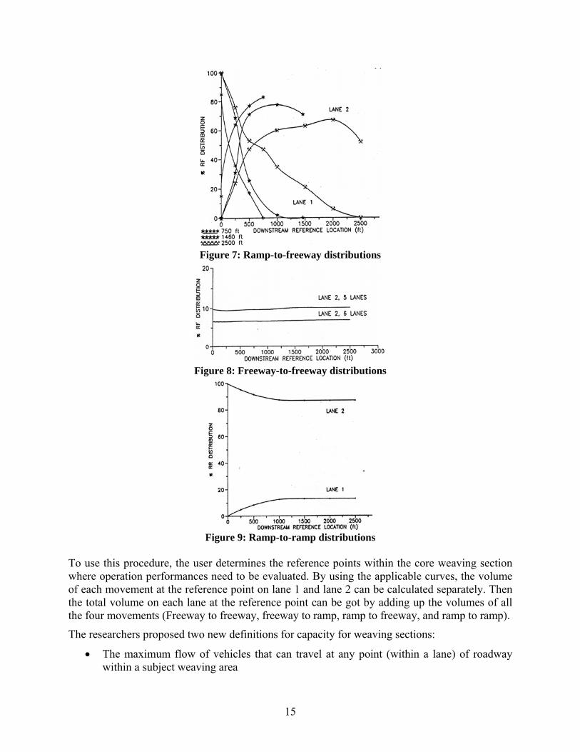
15

Figure 7: Ramp-to-freeway distributions

Figure 8: Freeway-to-freeway distributions

Figure 9: Ramp-to-ramp distributions

To use this procedure, the user determines the reference points within the core weaving section where operation performances need to be evaluated. By using the applicable curves, the volume of each movement at the reference point on lane 1 and lane 2 can be calculated separately. Then the total volume on each lane at the reference point can be got by adding up the volumes of all the four movements (Freeway to freeway, freeway to ramp, ramp to freeway, and ramp to ramp).

The researchers proposed two new definitions for capacity for weaving sections:

• The maximum flow of vehicles that can travel at any point (within a lane) of roadway within a subject weaving area

16

• The maximum rate of lane changing (between two adjacent lanes) that can occur over any 250-ft lane segment within the weaving area

The researchers used INTRAS as the simulation software to determine the values of capacity. The capacity threshold values were assumed to be reached when a little more input flows would cause a small number of weaving vehicles (1% or 2%) were unable to perform desired movements. 2200 pcphpl was obtained as the capacity flow at any point in the weaving section. Lane changing capacity across a single lane line over any 250-ft segment within the weaving section was found to range from 1,100 to 1,200 pcph.

The researchers recommended that density would be used to judge level of service of weaving sections because of its predictability and low scatter. It is found that the density at capacity is roughly 46 passenger cars per mile per lane.

Ostrom, Leiman, and May (1993) reported about an interactive computer program called FREWEV which incorporated the upper procedure, and called the procedure “point flow by movement”. The researchers also proposed another regression method called “total point flow method” to estimate the flow at any reference point along weaving section. It has the following form:

RReRFdFRcFFba ⋅+⋅+⋅+⋅+=ft XXat N lane in Flow [10]

Where a, b, c, d, e Constants

FF Freeway to freeway volume in pcph FR Freeway to off-ramp volume in pcph RF On-ramp to freeway volume in pcph RR On-ramp to off-ramp volume in pcph

In the upper equation, the coefficients can provide information on the influence of the component flows within a conflict area, but the coefficients do not represent the percentage of each movement at a specific analysis point. This is the major difference between point flow by movement method and total point flow method.

For a limited data base, the author compared the flow point by movement method, total point flow method, and Level D method. It was found that for major weaving sections, point flow by movement method got best results in terms of predicted volumes at reference points, while for ramp weaving sections, the total point flow method was proved to be most effective.

2.9 Fazio and Rouphail (1990, 1993) Fazio and Rouphail (1990) proposed conflict rates as a more effective measure of effectiveness (MOE) than weaving and nonweaving speeds estimated from 1985 HCM for one-sided freeway weaving sections. The researchers used conflict rates to quantify traffic turbulence on freeway weaving sections.

Two types of conflicts were identified in this study: lane change (LC) and read-end (RE) conflicts. In an LC conflict, the deceleration of the following vehicle in the target lane will range from coasting deceleration to the maximum deceleration that the vehicle can develop. Coasting

17

deceleration occurs when the driver removes his or her foot from the accelerator without applying the brakes.

A freeway RE conflict occurs when a vehicle slows or stops on a freeway and the driver of the following vehicle in the same lane reacts by applying the vehicle’s brakes to avoid collision.

According to the percentage of the maximum deceleration that is applied in a give situation, conflicts can be categorized into several severity levels, such as minor, moderate, and major.

The researchers identified two types of lane changes in weaving sections, including the lane changes made by weaving vehicles and the lane changes made by non-weaving vehicles. It is estimated that only a small portion of these lane changes results in LC conflicts. It was further pointed out that an LC conflicts might propagate additional LC and RE conflicts further upstream, and RE conflict might also result in further RE and LC conflicts upstream.

Conflict rate is calculated by dividing the number of conflicts by the total trip lengths by all the vehicles in core weaving section, expressed in conflicts per vehicle-mile.

The researchers modified the INTRAS simulation model to enable it to count conflict rates during simulation. Four conflict rates were identified, including total read-end conflict rate, total mandatory lane change conflict rate, and total lane change (mandatory + optional) conflict rate. It is found conflict rate MOEs had overall high sensitivity than speed MOEs to most operational variables such as length of weaving section, number of lanes, volume-to-capacity ratio, volume ratio (weaving volume to total volume), and weaving ratio (minor of the two weaving volume to total weaving volume).

Finally, the researchers proposed the following procedure to decide the LOS of weaving section:

1) Count RE and LC conflicts (e.g. brake light indications) that occur within the weaving section during the peak 15-min period.

2) During the same 15 min, count the number of vehicles entering the weaving section from the freeway and on-ramp.

3) Calculate the conflict rate by: Conflict rate = 15-min conflict count /(15-min volume *L/5280)

4) Determine weaving and non-weaving LOS for the one-sided weaving using Figure 10.

It is very reasonable that conflict rates can quantify the turbulences made to traffic flow. But using conflict rate to define level of service is not perfect since it is not consistent for nonweaving LOS, as can be seen in Figure 10.

In a later paper (Fazio, Holden, and Rouphail, 1993) the researchers reported the effort to studying the relationship between freeway conflict rates and safety. It was found that a correlation coefficient of 0.74 occurred between lane change conflict rates and reported angle/sideswipe crash rates, and a coefficient of 0.95 occurred between rear-end conflict rates and rear-end crash rates for the eight ramp weaving section that had moderate lengths ranging from 260 m to 305 m. For the examined other weaving sections beyond this length range, correlation between conflict rates and crash rates are not so evident. It was concluded that conflict rates provides an alternative to crash rates as an indicator of safety.

18

Figure 10: Overall conflict rate versus LOS for a simple one-sided weaving section

2.10 Wang, Cassidy, Chan, and May (1993) Wang, Cassidy, Chan, and May (1993) proposed an approach for evaluating the capacity of freeway weaving sections.

In this study, the data gathered for previous research (Cassidy, et al., 1989) for one Type B major weaving section. The INTRAS model was used to predict flows and lane-changing rates within the waving section. The researchers tried to identify the boundary between congested and uncongested operation by incrementally increasing input traffic demands over repeated simulations. The researchers relied on the error message issued by INTRAS when one or more vehicles in the traffic stream cannot execute desired maneuvers to reflect congested or “breakdown” conditions.

From the simulation results, the researchers found that a “functional value”, which can be expressed as “the total rate of vehicles that can occupy any portion of the critical region, can be used to clearly separate congested conditions from uncongested conditions crisply when the weaving section exhibits “typical” levels of weaving traffic demand. The functional value of capacity was identified to be 5,900 pcph for critical region.

In this study, the functional value was counted by summing up the through traffic volumes at the entrance of core weaving area and the number of lane changes in the critical region. Thus, the weaving vehicles were double counted.

When weaving area exhibits a relatively low level of weaving demands, the researchers recommended an average of 2,200 pcphpl among all the lanes on core weaving area as the capacity.

In this study, the researchers did some modifications to INTRAS. One modification was made to the lane changing criteria. In INTRAS, a risk number is calculated when a vehicle needs to change lane is faced with a potential gap on the neighboring lane. Whether the vehicle accepts the gap to change lane depends on if the risk number is bigger than acceptable risk. In the original INTRAS, the acceptable risk is a constant. The constant value was replaced by a

19

function that starts with a low value at the weaving section’s merge point, and increases as the vehicle progresses downstream.

One shortcoming of INTRAS was also reported in this study. In field, as total weaving flow rate increases, motorists traveling from freeway to ramp tend to execute required lane changes over shorter traveled distances. INTRAS, however, was unable to replicate these subtle motorist responses to varying flow conditions.

2.11 Windover and May (1994) Windover and May (1994) reported the efforts made to revise Level D methodology of analyzing freeway ramp weaving sections. The Level D method was developed by Caltrans in the early 1960s. The level D method is appropriate for ramp weaving and non-ram-weaving section operating under conditions of high or near-capacity traffic flow. Level D predicts the point flow at multiple locations along the two rightmost lanes as a sum of the individual movements. The RF and FR percentages in each lane at each location are solely a function of section length. It was point out that the errors in predicting the flow at points on the rightmost through lane was attributed principally to incorrect predictions of FF volumes.

The researchers came up with the following regression equation to estimate the percent of through traffic on the rightmost through lane.

FF% = 7.92 + 0.0117(LENGTH) – 0.00211(S1) – 0.00511(ON) + 0.0155(OFF) [11] Where

LENGTH Length of core weaving area in meter S1 Volume on upstream of freeway in pcph

ON On-ramp volume in pcph OFF Off-ramp volume in pcph

From the limited data base, the revised Level D method can estimate total point flow to the same level of accuracy as the former introduced total point flow method.

Following the publication of the 1985 HCM, several studies showed that the 1985 HCM procedure underestimated speeds in many sections for which data were available for verification. Roess, McShane, and Prassas (1998) updated the procedure, and it was later adopted for inclusion in the 1997 Update to HCM. Actually no big changes occurred in the update. 2.12 Fredericksen and Ogden (1994) Fredericksen and Ogden (1994) proposed an analytical procedure for analyzing Type A weaving sections on frontage roads. Since most of the researches on weaving section were limited to freeway, the researchers tried to address the behaviors of weaving on frontage roads. In this procedure lane change intensity (LCI) was used as the measure of effectiveness. It was expressed as:

section) weavingofgth lanes)(len ofnumber (hourper changes lane ofnumber LCI = [12]

LCI can be predicted by the following proposed regression models on the base of average volume per lane. They were calibrated for three groups of lengths of weaving sections.

20

400 ~ 599 ft: LCI = 10.46 (V/n) + 372 600 ~ 899 ft: LCI = 8.52 (V/n) + 79 900 ~ 1200 ft: LCI = 391 (V/n) + 590

Where: V Hourly volume entering weaving section n Number of lanes in weaving section

LCI can also be estimated by using Figure 11. According to LCI, the researchers denoted three levels of service including unconstrained, constrained, and undesirable. LOS can also be decided by using Figure 11.

Figure 11: Proposed LCI Models

2.13 Vermijs (1998) Vermijs (1998) developed a microscopic simulation approach for estimating weaving section capacities that was developed for the HCM equivalent in the Netherlands. The researcher identified four basic steps that should be considered within a weaving section, namely: gap searching, adjusting speed, executing a lane change, and adjusting the lead headway. It was further pointed out that when traffic flows on the weaving section are very low, the second and fourth steps are usually not executed. The researcher identified a number of factors that are critical in the analysis of weaving section capacities. These factors include the weaving section length, the Origin-Destination (O-D) pattern that enters the weaving section, the vehicle composition, and the entering speeds of vehicles from the on-ramp.

Since it is considered that the marginal effect of weaving cars on capacity is larger that the marginal effect of non-weaving cars, the researcher thought the effect of weaving vehicles on capacity is nonlinear and should have the following convex shape showed in Figure 12.

21

Figure 12: Shape of Capacity to Weaving Flow Rate Relationship

The researcher introduced the simulations done for Type A configurations, which are shown in Figure 13. In total 315 cases were identified regarding to configuration, weaving section length, weaving vehicle percentage in ramp flow, and percentage of trucks. All the simulation was finished in FOSIM (Freeway Operations SIMulation), which was developed in Netherlands. During a simulation, all input flows gradually increased until congestion occurred on a cross-section. Since FOSIM is a stochastic microscopic model, for every case 100 simulation runs were finished with different seeds.

Figure 13: Type A Configurations

For each case the 100 simulation results for capacity appeared to be normally distributed with standard deviation in the range of 200 ~ 400 vphpl.

The researcher also found that the pcu values for trucks are not the same for all configurations considered. The estimated pcu values are shown in Table 1.

Table 1: Estimated pcu Values for Weaving Sections Configuration 1+1 2+1 3+1 4+1 2+2 3+2 4+2 Pcu for trucks 2.5 3.1 3.2 3.6 2.7 2.8 2.9

2.14 HCM 2000 The 2000 HCM procedures, as did their processors, estimate the speed of the traffic stream in a weaving section as the harmonic mean of the weaving and non-weaving vehicles, as demonstrated in Equation 13. Subsequently, the weaving section density is computed using Equation 14. The level of service is then computed using the weighted average density for all vehicles in the weaving section or applied separately for weaving and non-weaving vehicles. The use of traffic density for estimating the LOS ensures consistency across all uninterrupted LOS procedures. However, the current HCM procedures set the density boundaries at higher levels than for basic freeway segments in order to account for the increased turbulence of the weaving area.

22

The 2000 HCM computes the speed of weaving and non-weaving vehicles separately, as demonstrated in Equation 15 using a weaving intensity factor that is computed in Equation 16. The constants of calibration in the weaving intensity factor (W) vary based on (1) whether the prediction is for speed of the weaving or non-weaving vehicles, (2) the configuration type (A, B, or C), and (3) whether the operation is constrained or unconstrained. The constrained mode of operation refers to a weaving section where the weaving vehicles utilize fewer lanes than is required for equilibrium. The number of lanes that are required for equilibrium is computed using Equations 17, 18, and 19 for Type A, B, and C configurations, respectively, while the maximum number of lanes that weaving vehicles can occupy is provided in the HCM as 1.4, 3.5, and 3.0 lanes for Type A, B, and C configurations, respectively. In the case that the Nw is less than or equal to Nw (max), the weaving section is considered to be unconstrained, otherwise it is considered to be constrained.

w

w

nw

nw

wnw

Sv

Sv

vvS

+

+= [13]

NSvD = [14]

ii W

SSS

+−

+=1

24 minmax [15]

d

cb

i LNvVRaW

)28.3()/()1(

⋅+

= [16]

( )438.0

234.0571.0 00328.019.2

ww S

LVRNN ⋅⋅⋅⋅= [17]

( )⎥⎦⎤

⎢⎣

⎡ −−+⋅+= wnww SSL

VRNN 018.06.71703.0085.0 [18]

( )[ ]wnww SSLVRNN −−⋅+⋅+= 005.0000011.0047.0761.0 [19]

23

Where: S Weighted average speed within the weaving section (km/h) D Weighted average density within the weaving section (veh/km) Si Average speed of vehicles (i = w for weaving vehicles, nw for non-weaving

vehicles) (km/h) Smax Maximum speed in weaving area (known as the free-flow speed) (km/h) Smin Minimum speed in weaving area (taken to be 16 km/h) Wi Weaving intensity factor (i = w for weaving vehicles and nw for non-weaving

vehicles) VR Ratio of weaving volume to total volume v Total demand flow on weaving section (veh/h) N Number of lanes on core weaving section L Length of weaving section (m) a, b, c, and d Constants of calibration Nw Number of lanes weaving vehicles must occupy to achieve equilibrium Nw (max) Maximum number of lanes that weaving vehicles can occupy based on the

configuration In addition, the Roess and Ulerio (2000) developed a procedure for estimating the capacity of the two weaving lanes adjacent to the crown line in a Type A weaving section using Equation 20. The basic logic behind the approach was to provide an analytical formula that converged to the capacity of a basic freeway section as the weaving volume approached zero. In addition, the logic hypothesized that the weaving section capacity increased as the weaving volume increased because, the claim was that drivers become more aggressive as the weaving intensity increases.

It should be noted that the model was rejected by the Highway Capacity and Quality of Service (HCQS) committee for two major reasons. First, the model was based on the principle that the capacity increased with increasing demand, which is counterintuitive. Second, the model indicated that the capacity of the weaving section was independent of the length of weaving section.

Currently, the 2000 HCM provides lookup tables (Exhibit 24-8) that provide estimates of weaving section capacities as a function of a number of variables, namely: the weaving section type, number of lanes, free-flow speed of freeway, length of weaving section, and volume ratio. The HCM recommends using straight line interpolation to compute weaving section capacities for intermediate values.

( )⎪⎪⎪

⎩

⎪⎪⎪

⎨

⎧

>∀⎟⎟⎠

⎞⎜⎜⎝

⎛ −⋅+−

≤≥∀<∀+

=

30002370

2142230012

3000,70030007002300

vv

VR

vvvv

cw

w

w

ww

w [20]

Where: cw Capacity of two weaving lanes (veh/h) VRw Ratio of weaving to total flow in weaving lane vw Total weaving flow in two weaving lanes (veh/h) v Total flow in two weaving lanes (veh/h)

24

2.15 Kwon, Lau, and Aswegan (2000) Kwon et al. (2000) developed an on-line procedure for estimating weaving section capacities. The study concluded that under free-flow conditions, the most significant factor affecting the speed of diverging vehicles is the geometric conditions of the exit ramp. Second, as the weaving volume increases, diverge vehicles tend to make lane changes earlier within the weaving section, while the ramp-to-freeway vehicles tend to travel a short portion on the auxiliary lane before merging into the mainline. Third, vehicles tend to use a limited portion of the auxiliary lane and that the length of the auxiliary lane utilization increases with increased weaving flows.

2.16 Lertworawanich and Elefteriadou (2001, 2003) Lertworawanich and Elefteriadou (2001) proposed a methodology to estimate the capacities of Type B weaving areas based on gap acceptance and linear optimization. A typical type B configuration is shown in Figure 14.

Figure 14: Type B Weaving Area with traffic flow rates at Capacity

The linear optimization model to calculate the capacity of the rightmost three lanes is as follows:

Capacity = max (VRR + VRF + VFF1 + VFR11 + VFR10 + VFR2 + VFF2) [21] Subject to:

Capacity constraint 1: VRR + VRF ≤ BFC Capacity constraint 2: VFF1 + VFR11 + VFR10 ≤ BFC Capacity constraint 3: VRF + VFF1 + VFR11 + VFR2≤ BFC Capacity constraint 4: VFR2 + VFF2 ≤ BFC Capacity constraint 5: VRR + VFR10 ≤ BFC Lanes 1 and 2 volume ratio constraint:

11221011

21011 WVVVVV

VVV

FFFFFRFRFR

FRFRFR =++++

++

Ramp volume ratio constraint: 0WVV

V

RRRF

RF =+

Bounds of VRR, VFF1, VFF2, VFR11: ≤ BFC Bounds of VFR10: VFR10 ≤ max (VFR10) Bounds of VRF: VRF ≤ max (VRF) Bounds of VFR2: VFR 2 ≤ max (VFR2)

Where:

25

VFF1 Through traffic flow rate on lane 1 at capacity

VFR11 The FR traffic flow rate on lane 1 without lane change at capacity VFR10 The FR traffic flow rate on lane 1 with lane change at capacity VFF2 Through traffic flow rate on lane 2 at capacity VFR2 Weaving flow rate from lane 2 to lane 1 at capacity VRF Weaving traffic flow rate from the ramp at capacity VRR RR flow rate at capacity W1 Volume ratio of traffic demand on freeway lanes 1 and 2 W0 Volume ratio of traffic demand on ramp lane

BFC Basic freeway segment capacity max (VFR10) Maximum possible lane changes from lane 1 to auxiliary lane at current flow

conditions max (VRF) Maximum possible lane changes from on-ramp to lane 1 at current flow

conditions max (VFR2) Maximum possible lane changes from lane 2 to lane 1 at current flow conditions

In order to use this methodology, firstly, traffic related parameters, traffic demands, and speeds of traffic on each lane should be colleted. Secondly, maximum possible lane changes are calculated by using probability functions. Finally, the linear optimization problem is solved to get the capacity on the rightmost three lanes at the core weaving area.

From calculation, the following two conclusions were drawn:

1) The capacity model shows that weaving traffic streams from the freeway and the ramp have different impact on the capacities of weaving area. The HCM 2000 procedure may bring in some errors for not differentiating these two volumes.

2) The models also shows that volume ratio of the traffic on auxiliary lane has more influence on capacity estimates than that of the traffic on lanes 1 and 2 up to a certain value.

It was addressed that the proposed methodology provides better estimation for capacity than the 2000 HCM procedure for the collected traffic data at the study site over a period of days.

There are a few assumptions in this procedure. The procedure makes a significant simplifying assumption. Specifically, the methodology assumes that Freeway-to-Freeway (FF) vehicles do not make any lane changes between lanes 1 and 2 within the weaving section. However, field data demonstrate many instances where this assumption is not necessarily true (Rakha and Zhang, 2004). Specifically, field data demonstrate that in some instances FF vehicles move from lane 1 to lane 2 as they travel along the weaving section in order to avoid the turbulence that is associated with travel on lane 1. It is also hard to consider the influence of heavy vehicles in this model.

The same researchers also presented a similar procedure for estimating capacity at ramp weaves (2003). These models are too theoretical and it neglects some basic factors that affect the capacity of weaving sections. For example, the length of weaving area is very critical for lane changes to take places, but it never appears in the model. Another disadvantage of these models is that they are not easy to apply since a lot of data needs to be collected and the calculation load is heavy.

26

Chapter 3. The INTEGRATION 2.30 Framework for Modeling Lane-Changing Behavior in Weaving Sections

(Transportation Research Record, No. 1883, 2004, pp. 140-149)

Rakha and Zhang

27

The INTEGRATION 2.30 Framework for Modeling Lane-Changing Behavior in Weaving Sections

Hesham Rakha (Corresponding Author) Associate Professor, Charles Via Department of Civil and Environmental Engineering Leader, Transportation Systems and Operations Group Virginia Tech Transportation Institute 3500 Transportation Research Plaza (0536) Blacksburg, VA 24061 Phone: (540) 231-1505 Fax: (540) 231-1555 E-mail: rakha@vtti.vt.edu

Yihua Zhang Graduate Research Assistant Virginia Tech Transportation Institute 3500 Transportation Research Plaza Blacksburg, VA 24061

Word count: 5,749 (words) + 1,750 (tables and figures) =7,499

Paper submitted for presentation and publication at the 83rd Transportation Research Board Meeting

Oct. 24, 2003

Rakha and Zhang

28

ABSTRACT The paper validates the effectiveness of the INTEGRATION 2.30 model for the analysis of weaving sections. The validation is conducted by comparing the lateral and longitudinal distribution of simulated and field observed traffic volumes categorized by O-D pair on nine weaving sections in the Los Angeles area. The results demonstrate a high degree of consistency between simulated and field observed traffic volumes within the weaving sections. Furthermore, the study demonstrates how the use of optional lane bias and lane changing parameters can enhance the consistency between the INTEGRATION results and field data. Overall the study demonstrates the flexibility of the INTEGRATION software for the modeling of weaving sections.

Key words: Lane changing, Weaving, and INTEGRATION model.

1. INTRODUCTION A number of microscopic simulation software have been developed as a cost effective means for evaluating alternative transportation initiatives prior to their field implementation. These microscopic software utilize car-following and lane-changing models as their modeling core in capturing both the longitudinal and lateral movement of vehicles along highways. The lane-changing models attempt to capture the lane distribution and lane changing behavior.

This paper examines and validates the lane changing behavior within the INTEGRATION microscopic simulation model, which is a commercially available state-of-the-art software. The objectives of this research effort are two-fold. First, the paper describes the INTEGRATION framework for modeling discretionary and mandatory lane changing behavior. Second, the paper validates the INTEGRATION framework by comparing traffic volume distributions across lanes within weaving sections against field observed data. The comparison provides very useful insights into the power of these analytical and simulation tools for the modeling of basic and complex weaving sections.

Following the introduction, a brief literature review of the state-of-the-art analytical and simulation tools for the analysis of weaving sections is presented. Subsequently, the lane changing logic incorporated within INTEGRATION is described in terms of modeling discretionary and mandatory lane changing behavior. Subsequently, the field data that were utilized for validation as well as the analysis results are presented followed by the summary and conclusions of the paper.

2. LITERATURE REVIEW OF WEAVING SECTION MODELING A limited number of publications have described and validated the use of microscopic simulation software for the modeling of weaving sections. Specfically, Zarean and Nemeth (1988) utilized WEAVSIM, a microscopic simulation model, to investigate the effect of the different arrival speeds on the operation of weaving sections. Subsequently, the researchers developed a regression model for the modeling of weaving sections based on the simulation results. The simulation results demonstrated that the speed differential between the mainline and on-ramp arrivals had a significant effect on the operation of weaving sections, which was not considered in the 1985 HCM procedure (Highway Capacity Manual, 1985).

Rakha and Zhang

29

Skabardonis et al. (1989) applied the INTRAS microscopic simulation model to evaluate the operation of a few major freeway weaving sections. INTRAS was modified to predict the speeds of weaving and non-weaving vehicles and applied to eight major freeway weaving sections. Vehicle speeds within the weaving section were compared to a few analytical procedures that included the 1985 HCM procedure, Leisch’s procedure (Leisch, 1985), JHK’s procedure (Reilly, 1984), Fazio’s Procedure (Fazio, 1986), and the Polytechnic Institute of New York (PINY) procedure (Pignataro, 1975). The researchers concluded that the INTRAS speed predictions were closer to the field measurements than the analytical procedure speed predictions. The researchers concluded that simulation tools could be utilized with field data to enhance existing state-of-the-art analytical procedures for the modeling of weaving section operations.

Fazio et al. (1990) proposed the use of vehicle conflicts as a measure of effectiveness for the modeling of weaving sections instead of traffic speed. A conflict was identified when the following vehicle decelerated to maintain a safe headway between it and the vehicle ahead of it. The researchers recorded the number of conflicts within INTRAS and concluded that the conflict rate could be a more effective measure of effectiveness for the analysis of weaving sections.

Stewart et al. (1996) evaluated the capability of INTEGRATION version 1.50 for the modeling of weaving sections. The study showed that both the 1985 HCM procedure and INTEGRATION offered identical conclusions for a given sample problem. However, the study demonstrated differences between the two approaches on critical design parameters of weaving sections. Specifically INTEGRATION identified the number of lanes in the core area as a critical factor in affecting a weaving capacity, which was not the case with the HCM procedures. Alternatively, while the HCM procedures demonstrated that the length of the core area was critical in the design of weaving sections, the INTEGRATION results demonstrated that this factor was critical for short lengths but was less critical as the weaving section length increased.

Vermijs (1998) reported on the efforts in developing the Dutch capacity standards for freeway weaving sections using FOSIM (Freeway Operations SIMulation), a microscopic simulation software developed in the Netherlands. Specifically, a total of 315 Type A weaving sections with different configuration and traffic factors were simulated. All simulation runs were repeated 100 times using different random seeds. The 100 simulation results for capacity appeared to be normally distributed with standard deviation in the range of 200 ~ 400 veh/h/lane.

Prevedouros and Wang (1999) compared the simulation results for large freeway and arterial networks using CORSIM, INTEGRATION, and WATSIM. The network that was analyzed included three merge areas, three diverge areas, one weaving area, and an arterial with 11 signalized intersections. It was found that after calibrations, all three software were able to replicate field-measured volumes to a high degree of consistency.

Skabardonis (2002) simulated the operation of eight real-world weaving sites in California under a wide range of operating conditions using CORSIM. The results indicated that CORSIM with default parameter values under-predicted the speeds in the weaving section by approximately 19% on average. After calibration, CORSIM reasonably replicated observed traffic operations on all weaving sites. Specifically, the predicted average speeds were within ±8 km/h for most of the studied sites.

Rakha and Zhang

30

3. OVERVIEW OF INTEGRATION LANE-CHANGING LOGIC INTEGRATION is a microscopic traffic simulation and assignment model that can represent traffic dynamics in an integrated freeway and traffic signal network. It has been successfully applied since the early 1990's in North America and Europe (Bacon, 1994, Gardes, 1993, Hellinga and Van Aerde, 1994, Marcus, 1995, Rakha et al., 1998, Rakha et al., 2000, Dion et al., In press, and Rakha and Ahn, 2004).

The lane changing logic within INTEGRATION considers both mandatory and discretionary lane changes. Mandatory lane changing takes place when the current lane ceases to be a feasible option, and the driver must shift to another lane in order to leave the road or to avoid a roadway exit. Discretionary lane changing occurs when the adjacent lane is perceived to provide for better driving conditions. This lane changing logic incorporates a gap acceptance process, where the size of an acceptable gap in the adjacent lane is a function of the vehicle’s speed, distance to the point where the lane change should be completed, and the time spent by an individual vehicle searching for a gap. This section describes the INTEGRATION logic for modeling both mandatory and discretionary lane changing behavior.

3.1. Discretionary Lane Changing Behavior

The INTEGRATION model computes the vehicle’s desired speed using a steady-state car-following model that is calibrated macroscopically using loop detector data (Van Aerde and Rakha, 1995; Rakha and Crowther, 2003; Rakha et al., 2004). The desired speed in the current lane is computed every deci-second based on the distance headway and speed differential between the leading and following vehicles. In order to determine whether a discretionary lane change should be made, the perceived speeds in the current lane, the adjacent lane to the left, and the adjacent lane to the right are compared every second. In addition, all lanes are scanned every 5 seconds in order to identify any potential gaps across multiple lanes. The INTEGRATION model considers a pre-specified bias for a vehicle to remain in the lane in which it is already traveling in by adding an inertia factor to the vehicle’s desired speed when computing its perceived speed. The use of such a bias factor reduces the number of unnecessary lane changes by increasing the attractiveness of the current lane. The attractiveness of the current lane is achieved using three factors, a relative speed factor (f3), an absolute speed factor (f4), and a maximum inertia threshold (f5), as demonstrated in Equation 1. Figure 1 illustrates the INTEGRATION default parameters and the variation in the lane inertia factor as a function of the lane desired speed, as computed from the car-following model, and the vehicle length Passenger Car Unit (PCU) equivalency. The figure clearly demonstrates that the inertia factor increases as the desired speed increases through the use of the relative factor (f3) which encourages vehicles to make more lane changes at low speeds in order to minimize queue lengths at a signalized intersection. Furthermore, the inertia factor increases as the vehicle PCU increases. The use of the vehicle length equivalency factor within the inertia factor ensures that trucks make less lane changes than passenger cars.

In addition, the INTEGRATION model incorporates a bias towards travel in specific lanes depending on the number of lanes on the roadway when vehicles travel outside the influence area of merge and diverge sections. Specifically, the model biases passenger cars to travel towards the middle lanes for roadways with three or more lanes, as demonstrated in Figure 1. This bias is achieved by altering the perceived speed in a specific lane using the formula of Equation 2 in an attempt to achieve field observed traffic volume distributions across roadway lanes, as was

Rakha and Zhang

31

characterized by Carter et al., (1999). In addition, the model biases trucks towards use of the shoulder lane through the passenger car unit (pcu) vehicle length equivalency factor, as demonstrated in Figure 1.

pcufffuuu cci ),min(~543 ++= [1]

( ) ( )1712

1ABS2

~2

87 −⎟⎠⎞

⎜⎝⎛ −

++⎟⎟⎠

⎞⎜⎜⎝

⎛⎟⎠⎞

⎜⎝⎛ −+

−−+= pcu

niffuinnuu iii [2]

Where: uc = Vehicle speed in current lane (km/h), ũi = Perceived speed in lane “i” (km/h), ui = Actual speed in lane “i” (km/h), f3 = Relative inertia factor (unitless), f4 = Absolute inertia factor (km/h), f5 = Absolute inertia factor (km/h), f7 = Relative speed factor (unitless), f8 = Absolute speed factor (km/h), pcu = Vehicle length equivalency factor (e.g. a factor of 3.0 indicates that the length of the

vehicle is equivalent to the length of 3 passenger cars), and n = Number of lanes on roadway section

It should be noted that the INTEGRATION software allows users to override the default lane bias parameters using the optional 'lanebias.dat' input file. Specifically, the user can specify the degree of attractiveness of a lane using a divisive speed bias factor. For example, if the user specifies a factor of 3.0 the perceived speed on all lanes other than the biased lane is computed as 1/3 the desired speed, which is computed using the car-following logic. The “lanebias.dat” file allows the user to identify link-specific bias factors that are only effective on the links that are coded in the optional file. Once the vehicle leaves the link the default bias factors become effective. Consequently, if the user wants to maintain a user-specified bias over a number of links, a separate entry is required for each of the links.

3.2. Mandatory Lane Changing Behavior

In situations where a trip destination imposes a constraint on vehicle movement, for example, exiting vehicles at a ramp-freeway diverge section, mandatory lane changes are performed to ensure that vehicles maintain lane connectivity at the end of each link. This lane connectivity at any diverge or merge point is computed internal to the model rather than explicitly coding this as an input to the model. In order to briefly explain the mechanism of the mandatory lane changing logic within INTEGRATION, a simple configuration of a freeway diverge section in the proximity of an exit ramp is considered for this purpose, as shown in Figure 2.

Prior to reaching the physical diverge point, the obligatory lane changing logic in INTEGRATION assigns two imaginary boundaries upstream of the diverge gore. The first boundary, located farther upstream, is denoted as "softwall"; while the second boundary is denoted as "hardwall" and is located closer to the physical diverge point. While the hardwall indicates the location where exiting vehicles are unable to proceed closer to the diverge section on the original lane and thus must abandon the lane due to lane discontinuity downstream; the softwall defines the location where the

Rakha and Zhang

32

driver recognizes the need to change lanes in order to exit at a diverge section. The distance between these two boundaries represents a transition from the absolute discretionary nature to the absolute mandatory nature for the vehicle under consideration.

In order to ensure the smooth transition of flows from one lane to the next, the mandatory lane changing logic within INTEGRATION has been made highly stochastic rather than purely deterministic. This is reflected by the significant variation in the locations of the softwalls and the hardwalls upstream of the diverge gore. Within INTEGRATION, the mean locations of the softwalls are at a distance of 100n times the jam density distance headway upstream of the diverge gore, where n is the minimum number of lane changes required to complete the maneuver. Likewise, the mean locations of the hardwalls are at a distance of 10n times the jam density distance headway back from the point of diverge, where n is as defined earlier. This implies that, some very cautious drivers will strive to be in the rightmost lane a considerable distance upstream of the diverge gore. The locations of these imaginary boundaries were set based on engineering judgment and extensive testing of the model for different traffic and roadway conditions. It should be noted, however, that the user can alter the default lane change parameters that are incorporated within the INTEGRATION software by using an optional input file named “lanechange.dat”. This optional file provides the user with some degree of control over the lane changing behavior within the simulation model using global customization parameters.

In addition, the INTEGRATION model considers a mean default lane change duration of 2 seconds that again can be altered by the modeler via the “lanechange.dat” file. Currently, the model does not reduce the lane change duration depending on the number of lane changes that the driver has to make nor does it alter the duration depending on the urgency of the lane changing maneuver. Further research is required to attempt to characterize lane changing behavior as a function of the number of lane change maneuvers, the urgency of the lane change maneuver, and the level of congestion on the roadway.

A commonly observed phenomenon at merge and weaving sections is the movement of mainline vehicles from the shoulder lane to the middle and median lanes in order to avoid any interaction with merging vehicles. This behavior can be captured within the INTEGRATION software using the optional “lanebias.dat” file that was described earlier. Specifically, the use of a factor of 2.0, which results in a perceived speed that is half the actual speed on the surrounding lanes provides a good level of movement of vehicles from the shoulder lane to other lanes. Specifically, a factor of 2.0 entices vehicles to use the desired lane at low volumes; however, it has a minor effect at high volumes. As was the case with the soft and hardwalls the location at which vehicles respond to the specified bias is varied randomly across the different vehicles in order to ensure that not all lane changing occurs at the same location.

In INTEGRATION, if the values of the above mentioned parameters are not set explicitly, the values of f3, f4, f5, f7, and f8, are set to 0.2, 5 km/h, 10 km/h, 0.01, and 1.0 km/h respectively by default and the values of hardwall location factor and softwall location factor are both set to 10 and 100n (computed as 10×10). And the default lane changing duration is 2 seconds.

4. FIELD DATA This study utilized an empirical data set that was gathered in the late 1980's by University of California at Berkeley (Cassidy et al., 1990). Specifically, vehicle spatial distributions both total

Rakha and Zhang

33

and by movement, at successive reference points on nine weaving sites were gathered. The traffic movements included the four possible movements on freeway weaving sections, namely, Freeway-to-Freeway (FF), Freeway-to-Ramp (FR), Ramp-to-Freeway (RF), and Ramp-to-Ramp (RR). The volume counts were provided at 5-min intervals at a few reference points along the core weaving area.

It is important to point out that the empirical data included some misleading data due to special conventions used in the data collection process. Specifically, the length of a weaving section was defined as the distance from the tip of the painted merge gore point to the tip of the painted diverge gore point. This length was shown, in some cases, to be significantly different from that between the physical merge and diverge points. This issue will be addressed further in section 6.

Due to space limitation, only the analysis results of sites C1 and C8 are presented in this paper. The geometric layouts and other details are shown in Figure 3. Six hours of volume data were available for both the sites, including two hours for morning peak, the noon period, and the evening peak periods.

5. METHODOLOGY Geometric characteristics and traffic conditions at the investigated sites were input to INTEGRATION. In order to produce similar statistics to those of the field data, simulated loop detector stations were installed to match the location of the reference points in the field and polling intervals were set at 5-minute intervals. Field volume counts were input to the simulation model as O-D demands.

Because 20-s loop detector data were not available, the steady-state car-following parameters in INTEGRATION were selected to reflect typical freeway and ramp sections. Specifically, the basic freeway roadway capacity and free-flow speed were based on recommendations in chapter 13 of the 2000 HCM (TRB, 2000). The speed-at-capacity was selected to be 80 percent of the free-speed as suggested in the literature (Rakha and Crowther, 2003). Freeway Jam density and the corresponding parameters for ramp sections were specified based on judgment. Specifically, the capacity, speed-at-capacity, and free-flow speed for freeway segments were set to be 2,250 pcph, 93 km/h and 112 km/h respectively, while the corresponding settings for ramps were 1,800 pcph, 65 km/h and 80 km/h. The jam density was set at 125 pc/km/lane for both the ramps and freeway segments.

The traffic counts in the field data included heavy vehicles (trucks, buses, and recreational vehicles). These vehicles were explicitly modeled as trucks by considering truck vehicle dynamics and assumed to have a vehicle length equivalency factor of 3.0.

The first objective of the study was to investigate the robustness of the INTEGRATION model to capture the weaving behavior using the default lane bias and lane changing parameters. Subsequently, an attempt was made to enhance the model behavior by fine-tuning some of the lane bias and lane changing parameters. Specifically, in some cases the lane distribution of the mainline vehicles entering the weaving section was fine-tuned to better reflect the local traffic conditions. In addition, changes in two of the lane changing parameters were also investigated, including the locations of the softwalls and hardwalls, which will be discussed further in the paper.

Rakha and Zhang

34

6. ANALYSIS OF RESULTS This section presents the results of the model validation effort. These results are compared in terms of lane-specific O-D demands because these data were available in the field. Unfortunately, vehicle speed data were not available so it was impossible to compare the results in terms of average speeds across different lanes and movements. Initially, the results for the base case default parameter runs are presented. Subsequently, results are presented for cases in which some of the lane bias and lane changing parameters were altered in order to better match field conditions.

Figure 4 through Figure 6 illustrate the spatial variation in FF, FR, RF, and RR volumes on the shoulder and auxiliary lane(s) at all sites for a sample of time intervals for field data and as predicted by the INTEGRATION simulation model. It is important to mention that the slopes of the broken lines shown in these figures are an approximate indicator of the lane changing activity between any two successive reference points.

The first row of graphs within each figure demonstrates the spatial variation in total volume on the shoulder and auxiliary lane(s). The figures clearly demonstrate a high level of consistency between field data and the simulation results (minor differences between field and simulation results). These results clearly demonstrate that the INTEGRATION software is capable of modeling weaving sections using default lane bias and lane changing parameters.

In addition, each figure demonstrates the breakdown of O-D demands across the shoulder and auxiliary lane(s). Specifically, the field and simulated FF, FR, RF, and RR movements across the shoulder and auxiliary lane(s) are illustrated and compared.

6.1. Simulation Results for Default Parameters

At site C1, the traffic is characterized by a dominant diverge demand, as demonstrated in Figure 4. Specifically, the diverge volumes are approximately five to twenty times more than the corresponding merge volumes. The simulation results for site C1 demonstrate that the FF movement across the two lanes is consistent with field observations. Specifically, on the shoulder lane, the field observed FF movement is slightly higher than that estimated by the simulation model (error of 3 percent). The figure also demonstrates a consistency in the spatial variation trends across the two rightmost lanes. It is notable that on the auxiliary lane, at location 0 meter downstream the merge gore the FR traffic is 135 veh/h, rather than zero, implying that vehicles were able to change lanes prior to crossing the painted merge gore area. Alternatively, the simulation model does not allow vehicles to make lane changes prior to the gore area. Consequently, the difference in the FR volumes can be attributed to identifying the exact location of the point at which vehicles can start making lane changes. A comparison of the FR volume distribution across the shoulder and auxiliary lanes demonstrates that vehicles were biased towards the use of the auxiliary lane, while the simulation model demonstrated a more evenly distribution across the two lanes. It is not clear, at this point, if any potential desired turning movements at the downstream end of the off-ramp contributed to driver biases towards the auxiliary lane, which was not reflected within the simulation runs. Alternatively, the RF field volume distribution demonstrates that most of the lane changing activities occurs between the second and third reference points (i.e. between 76.2 and 152.4 m downstream the merge gore). However, the simulation software models a more uniformly distributed lane changing activity along the weaving section. Since the RF volume constitutes only 5 percent of the total traffic volume, this discrepancy should not affect the simulation results

Rakha and Zhang

35

significantly. The field and simulation results demonstrate a bias towards the auxiliary lane for RR volume, however the field results indicate that a number of vehicles shift lanes to the shoulder lane as they travel towards the off-ramp. Alternatively, the simulation results indicate that vehicles typically maintain their lane selection given that there is no incentive to make any lane changes.

Sites C8 is classified as type C according to the HCM 2000 procedures. On site C8 auxiliary lane 1 continues to the downstream mainline while auxiliary lane 2 only provides access to the off-ramp, as illustrated in Figure 3. The configuration of site C8 forces FR vehicles to make at least two lane changes along the core area while RF vehicles in auxiliary lane 1 do not have to make any lane changes. As for the O-D demand, the site is traveled by a low FR and RR demand and a high RF demand. The results for the PM peak demonstrate some discrepancies between field observed and simulated results, as demonstrated in Figure 5. Specifically, while in the case of the FR volume allocation the field observations and simulation results demonstrate that vehicles move into the shoulder lane prior to entering the core area, within the simulation model vehicles shift to auxiliary lane 2 earlier than is observed in the field. In the case of the RR movement, the simulated vehicles are almost evenly distributed on the two auxiliary lanes as they enter the core area, however the field data demonstrate a bias towards auxiliary lane 2, which would appear more realistic given that auxiliary lane 1 does not provide any access to the off-ramp. Consequently, it appears that the use of the lane bias file could enhance the operation of the RR movement by shifting some of the RR demand from auxiliary lane 1 to auxiliary lane 2 prior to entering the core area. Finally, in the case of the RF movement the field observations indicate that the RF vehicles are biased towards auxiliary lane 1 while the simulated vehicles are almost evenly distributed between the shoulder lane and auxiliary lane 1.

The results generally demonstrate a good match between the distribution of traffic demands across the various lanes except for some minor instances in which the simulation model does not capture driver biases towards specific lanes prior to entering the weaving section core area. The following sections will demonstrate how the use of the optional lane bias and lane change files can enhance the model operations to match field observations more accurately.

6.2. Lane Bias Adjustment Scenarios

From the previous analysis it was demonstrated that at site C8 the INTEGRATION model did not capture the vehicle lane distribution that occurs prior to entering a weaving section very well. The accurate modeling of lane distribution prior to entering the core area can have a significant impact on the operation of a weaving section. Consequently, this section demonstrates how the use of the optional lane bias file can be utilized to enhance the modeling capabilities. Specifically, the lane bias is applied to the upstream mainline and on-ramp sections in order to pre-segregate the vehicles prior to entering the weaving section in order to match field data more accurately. The simulation results are introduced to Figure 5 in order to make a direct comparison across the various simulation scenarios and to field data.

A comparison of the two series of simulation results in Figure 5 clearly demonstrates the improvement in simulation results that are achieved by utilizing the customized lane bias file. The figure clearly demonstrates that the use of the lane bias file results in an improved match between field and simulated results especially at the entrance to the core area. For example, Figure 5 demonstrates an improved lane distribution of the FF and RF demand at site C8.

Rakha and Zhang

36

6.3 Softwall and Hardwall Adjustment Scenarios

In order to study the influence of the hardwall and softwall locations on the traffic volume distribution within the weaving section a sensitivity analysis was conducted. Specifically, the hardwall and softwall location factor were varied between from 5 to 15 at increments of 2 and applied to the C8 site using the PM peak O-D table. As stated earlier, these factors characterize the number of jam densities upstream the downstream gore of the weaving section that the vehicle encounters the hardwall and softwall. For example, in the case of a factor of 5 for both the hardwall and softwall, the vehicle will encounter the hardwall 5 jam density headways upstream the gore for each required lane change. Alternatively, the vehicle will encounter the softwall 25 (5x5) jam density headways upstream the gore for each required lane change.

Figure 6 demonstrates the effects of softwall and hardwall adjustments. In the figure the “INTEGRATION 1” series represent a factor of 5, while the “INTEGRATION 2” series represents a factor of 15. Figure 6 clearly demonstrates a significant change in the FR distribution across the three lanes with different factor values. Specifically, a factor of 15 results in lane changes that occur early within the core area similar to what is observed in the field; while the use of a factor of 5 results in lane changes that occur further downstream along the core area. These results clearly demonstrate the flexibility of the tool in changing the locations at which vehicles make lane changes within a weaving section, thus providing the user with a number of calibration parameters that can be fine-tuned to the specific roadway and driver characteristics.

6.4 Quantification of Simulation Errors

In order to quantify the differences between simulation results and field data, the percentage simulation error at each reference point on a lane was computed using the following formula:

Percentage of simulation error = %100ˆ ×⎟⎟⎠

⎞⎜⎜⎝

⎛⎟⎟⎠

⎞⎜⎜⎝

⎛− ∑∑

ii

iii qqq [3]

Where: i = FF, FR, RF and RR demands,

iq = simulated volume for movement i, and iq = field observed volume for movement i.

The simulation error for the various simulation runs are summarized in Table 1. The maximum error across all shaded cells is 24.7 percent with an average error of 15.5 percent. This margin of error falls within the normal range of daily variability that is observed in field data (Rakha and Van Aerde, 1995). Consequently, the results for the nine weaving sections demonstrate that the INTEGRATION software provides a reasonable degree of accuracy for the modeling of weaving sections. Clearly, more testing is required to validate the model estimates of vehicle speeds within weaving sections.

Noteworthy is the fact that for the auxiliary lane of site C1, the “premature” lane changes that occur upstream of the merge gore contribute significantly to the differences that are observed between field data and simulation results, demonstrating that lane markings may not reflect actual gore locations.

Rakha and Zhang

37

7. SUMMARY AND CONCLUSIONS The research presented in this paper examined one of the most important components of microscopic traffic simulation models, namely the lane-changing logic. Specifically, the lane changing logic within the INTEGRATION software was presented and validated against field data collected on nine different freeway weaving sections (only two of them are presented in this paper). In this study, the vehicle demand distribution, both total and by movement, across the weaving lanes were compared in order to validate the lateral and longitudinal lane changing activity logic.

The analysis demonstrated that the lane changing behavior within a weaving section is a very complicated phenomenon that is affected by many factors including the geometric configuration of the weaving section and the O-D demand.

The results demonstrate good agreement between the simulation results and the field data. In the cases that the results did not agree it appeared that the vehicle distribution prior to entering the weave section was critical. The study demonstrated how the use of optional lane bias and lane changing parameters can enhance the consistency between the INTEGRATION results and the field data. In conclusion, it appears that the INTEGRATION model offers a robust tool for the modeling and evaluation of weaving sections.

REFERENCES Bacon, V., et al., Use of INTEGRATION Model to Study High-Occupancy-Vehicle Facilities,

Transportation Research Record No. 1446, 1994, pp. 8-13.

Cassidy, M., Chan, P., Robinson, B., and A. D. May, A Proposed Analytical Technique for the Design and Analysis of Major Freeway Weaving Sections, Institute of Transportation Studies, University of California-Berkeley, research Report UCB-ITS-RR-90-16. 1990.

Dion F., Rakha H., and Zhang Y. (In press), Evaluation of Potential Transit Signal Priority Benefits Along a Fixed-Time Signalized Arterial. ASCE Journal of Transportation Engineering.

Fazio, J. and Rouphail, N. M. Conflict Simulation in INTRAS: Application to Weaving Area Capacity Analysis, Transportation Research Record. n 1287, 1990, pp. 96-107.

Fazio, J. and Rouphail, N. M., Freeway Weaving Sections: Comparison and Refinement of Design and Operations Analysis Procedures, Transportation Research Record, n 1091 1986, pp. 101-109.

Gardes, Y. and A.D. May. Simulation of IVHS on the Smart Corridor Using the INTEGRATION Model: Initial Investigation. PATH Research Report, UCB-ITS-PRR-93-3, 1993.

Hellinga, B., and Van Aerde, M., An Overview of a Simulation Study of the Highway 401 Freeway Traffic Management System, Canadian Journal of Civil Engineering, Vol. 21, 1994.

Leisch, J. E. et al. Procedure for Analysis and Design of Weaving Sections. Report FHWA/RD-85/083, FHWA, U.S. Department of Transportation, 1985.

Rakha and Zhang

38

Pignataro, L. J. et al., NCHRP Report 159: Weaving Areas — Design and Analysis, Polytechnic Institute of New York, TRB, National Research Council, Washington, D.C., 1975.

Prevedouros, P. and Wang, Y., Simulation of Large Freeway and Arterial Network with CORSIM, INTEGRATION, and WATSim, Transportation Research Record, n 1678, 1999, pp. 197-207.

Rakha H. and Van Aerde M., Statistical Analysis of Day-to-Day Variations in Real-Time Traffic Flow Data, Transportation Research Record, No. 1510, pp. 26-34, 1995.

Rakha, H., Van Aerde, M., Bloomberg, L., and X. Huang, Construction and Calibration of a Large-Scale Micro-Simulation Model of the Salt Lake Area, Paper presented at the 77th Transportation Research Board Annual Meeting, Washington, D.C., January 11-15, 1998.

Rakha H., Medina A., Sin H., Dion F., Van Aerde M., and Jenq J. (2000), Coordination of Traffic Signals Across Jurisdictional Boundaries: Field and Simulation Results, Transportation Research Board 79th Annual Meeting, Washington DC, January, CD-ROM [Paper # 00-1560].

Rakha H. and Lucic I. (2002), Variable Power Vehicle Dynamics Model for Estimating Maximum Truck Acceleration Levels, ASCE Journal of Transportation Engineering, Vol. 128(5), Sept./Oct., pp. 412-419.

Rakha H. and Crowther B. (2003), Comparison and Calibration of FRESIM and INTEGRATION Steady-state Car-following Behavior, Transportation Research, 37A, pp. 1-27.

Rakha H., Pasumarthy P., and Adjerid S. (2004), Car-Following Models: Formulations, Issues, and Practical Considerations, Submitted to the Journal of Transportation Research.

Rakha H. and Ahn K. (2004), The INTEGRATION Modeling Framework for Estimating Mobile Source Emissions. ASCE Journal of Transportation Engineering, March Issue.

Reilly, W., Kell, J. H., and Johnson, P. J., Weaving Analysis Procedures for the New Highway Capacity Manual, JHK and Associates, 1984.

Skabardonis, A., Simulation of Freeway Weaving Areas, Transportation Research Record, n 1802, 2002, pp. 115-124.

Skabardonis, A., Cassidy, M., May, A. D., and Cohen, S., Application of Simulation To Evaluate the Operation of Major Freeway Weaving Sections, Transportation Research Record, n 1225, 1989, pp. 91-98.

Special Report 209: Highway Capacity Manual. TRB, National Research Council, Washington, D.C., 1985.

Stewart, J. Baker, M. Van Aerde, M. Evaluating Weaving Section Designs Using INTEGRATION, Transportation Research Record, n 1555, 1996, pp. 33-41.

M. Van Aerde & Assoc., Ltd., INTEGRATION Release 2.30 for Windows: User’s Guide, Van Aerde and Associates Ltd.

Vermijs, R., New Dutch Capacity Standards for Freeway Weaving Sections Based on Micro Simulation, Third International Symposium on Highway Capacity, 1998, pp. 1065-1080.

Rakha and Zhang

39

Zarean, M. and Nemeth, Z. A., WEASIM: A Microscopic Simulation Model of Freeway Weaving Sections, Transportation Research Record, n 1194, 1988, pp. 48-54.

Rakha and Zhang

40

Table 1: Quantifying the Differences between Simulation Results and Field Data Site & Period Lane Scenario 1st point 2nd point 3rd point 4th point

Shoulder lane Default 12.6% 19.6% 21.9% 21.4%

Default 30.6% 34.6% 32.2% 32.7% Site C1, AM Auxiliary lane

Default* 0.3% 22.0% 22.2% 24.1% Default 44.1% 39.7% 33.5% 28.8%

Shoulder lane With lane bias 8.2% 17.8% 17.0% 13.5%

Default 41.9% 21.9% 19.0% 3.0% Auxiliary lane 1

With lane bias 24.7% 16.2% 14.4% 7.6%

Default 39.4% 26.8% 27.5% 15.3%

Site C8, PM

Auxiliary lane 2 With lane bias 1.6% 20.0% 9.9% 14.3%

* The results are obtained from simulation with default parameter values, while the influence of erroneous FR volume at location 0 was removed.

Rakha and Zhang

41

f3 0.2f4 5f5 10f7 0.01f8 1

0

5

10

15

20

25

0 20 40 60 80 100 120

Desired Speed in Current Lane (km/h)

Iner

tia F

acto

r (km

/h)

PCU=1 PCU=2 PCU=3 PCU=4 PCU=5

PCU = 1.0

0

10

20

30

40

50

60

70

80

90

2 3 4 5 6

Number of Lanes

Perc

eive

d Sp

eed

(km

/h)

Lane 1Lane 2Lane 3Lane 4Lane 5Lane 6

PCU = 3.0

0

10

20

30

40

50

60

70

80

90

2 3 4 5 6

Number of Lanes

Perc

eive

d Sp

eed

(km

/h)

Lane 1Lane 2Lane 3Lane 4Lane 5Lane 6

Figure 1: INTEGRATION Default Lane Bias Features

hwj : hardwall locationswj : softwall location

hw2

hw1

sw1

sw2Lane 2

Lane 1

Figure 2: Hardwall and Softwall Locations at a Sample Diverge Section

Rakha and Zhang

42

Shoulder lane Auxiliary lane

445 m

Site C1 (Type B)

Shoulder lane

Auxiliary lane 1 Auxiliary lane 2

369 m

Sites C8 (Type C)

Site names (in symbols) are the same as those that appear in the original report.

Figure 3: Test Site Weaving Section Configurations.

Rakha and Zhang

43

Shoulder Lane Auxiliary Lane

0

500

1000

1500

2000

0 50 100 150 200 250 300 350

Location Downstream of Merge Gore (m)

FR V

olum

e (v

eh/h

)

0

50

100

150

200

0 50 100 150 200 250 300 350

Location Downstream of Merge Gore (m)

RF

Volu

me

(veh

/h)

0

50

100

150

200

0 50 100 150 200 250 300 350

Location Downstream of Merge Gore (m)

RR

Vol

ume

(veh

/h)

0

100200300

400500600

0 50 100 150 200 250 300 350

Location Downstream of Merge Gore (m)

FF V

olum

e (v

eh/h

)

0100

200300

400500600

0 50 100 150 200 250 300 350

Location Downstream of Merge Gore (m)

FF V

olum

e (v

eh/h

)

0

500

1000

1500

2000

0 50 100 150 200 250 300 350

Location Downstream of Merge Gore (m)

FR V

olum

e (v

eh/h

)

0

50

100

150

200

0 50 100 150 200 250 300 350

Location Downstream of Merge Gore (m)

RF

Volu

me

(veh

/h)

0

50

100

150

200

0 50 100 150 200 250 300 350

Location Downstream of Merge Gore (m)

RR

Vol

ume

(veh

/h)

0

500

1000

1500

2000

2500

0 50 100 150 200 250 300 350

Location Downstream of Merge Gore (m)

Tota

l Vol

ume

(veh

/h) Field

INTEGRATION

0

500

1000

1500

2000

2500

0 50 100 150 200 250 300 350

Location Downstream of Merge Gore (m)

Tota

l Vol

ume

(veh

/h) Field

INTEGRATION

Average flows (pcph) FF: 5208 FR: 2241 RF: 148 RR: 166

Figure 4: Site C1 Volume Comparison (AM Period – Default Lane-Changing Parameters)

Rakha and Zhang

44

Shoulder Lane Auxiliary Lane 1 Auxilary Lane 2

0

100

200

300

400

500

0 50 100 150 200 250 300 350

Location Downstream of Merge Gore (m)

FR V

olum

e (v

eh/h

)

0

500

1000

1500

2000

2500

0 50 100 150 200 250 300 350

Location Downstream of Merge Gore (m)

RF

Volu

me

(veh

/h)

0

50

100

150

200

250

300

0 50 100 150 200 250 300 350

Location Downstream of Merge Gore (m)

RR

Vol

ume

(veh

/h)

0

500

1000

1500

0 50 100 150 200 250 300 350

Location Downstream of Merge Gore (m)

FF V

olum

e (v

eh/h

)

0

500

1000

1500

0 50 100 150 200 250 300 350

Location Downstream of Merge Gore (m)

FF V

olum

e (v

eh/h

)

0

100

200

300

400

500

0 50 100 150 200 250 300 350

Location Downstream of Merge Gore (m)

FR V

olum

e (v

eh/h

)

0

500

1000

1500

2000

2500

0 50 100 150 200 250 300 350

Location Downstream of Merge Gore (m)

RF

Volu

me

(veh

/h)

0

50

100

150

200

250

300

0 50 100 150 200 250 300 350

Location Downstream of Merge Gore (m)

RR

Vol

ume

(veh

/h)

0

500

1000

1500

2000

2500

0 50 100 150 200 250 300 350

Location Downstream of Merge Gore (m)

Tota

l Vol

ume

(veh

/h)

FieldINTEGRATION (Default)INTEGRATION (W/ lanebias)

0

500

1000

1500

2000

2500

0 50 100 150 200 250 300 350

Location Downstream of Merge Gore (m)

Tota

l Vol

ume

(veh

/h)

FieldINTEGRATION (Default)INTEGRATION (W/ lanebias)

0

500

1000

1500

2000

2500

0 50 100 150 200 250 300 350

Location Downstream of Merge Gore (m)

Tota

l Vol

ume

(veh

/h) Field

INTEGRATION (Default)INTEGRATION (W/ lanebias)

0

500

1000

1500

0 50 100 150 200 250 300 350

Location Downstream of Merge Gore (m)

FF V

olum

e (v

eh/h

)

0

100

200

300

400

500

0 50 100 150 200 250 300 350

Location Downstream of Merge Gore (m)FR

Vol

ume

(veh

/h)

0

500

1000

1500

2000

2500

0 50 100 150 200 250 300 350

Location Downstream of Merge Gore (m)

RF

Volu

me

(veh

/h)

0

50

100

150

200

250

300

0 50 100 150 200 250 300 350

Location Downstream of Merge Gore (m)

RR

Vol

ume

(veh

/h)

Average traffic flows (pcph) FF: 6055 FR: 409 RF: 3372 RR: 265

Figure 5: Site C8 Volume Comparison (PM Period, Default Lane-Changing Parameters vs. Lane

Bias on Upstream Mainline and On-ramp)

Rakha and Zhang

45

Shoulder Lane Auxiliary Lane 1 Auxilary Lane 2

0

100

200

300

400

500

0 50 100 150 200 250 300 350

Location Downstream of Merge Gore (m)

FR V

olum

e (v

eh/h

)

0

500

1000

1500

2000

2500

0 50 100 150 200 250 300 350

Location Downstream of Merge Gore (m)

RF

Volu

me

(veh

/h)

0

100

200

300

0 50 100 150 200 250 300 350

Location Downstream of Merge Gore (m)

RR

Vol

ume

(veh

/h)

0

200

400

600

800

1000

0 50 100 150 200 250 300 350

Location Downstream of Merge Gore (m)

FF V

olum

e (v

eh/h

)

0

200

400

600

800

1000

0 50 100 150 200 250 300 350

Location Downstream of Merge Gore (m)

FF V

olum

e (v

eh/h

)

0

100

200

300

400

500

0 50 100 150 200 250 300 350

Location Downstream of Merge Gore (m)

FR V

olum

e (v

eh/h

)

0

500

1000

1500

2000

2500

0 50 100 150 200 250 300 350

Location Downstream of Merge Gore (m)

RF

Volu

me

(veh

/h)

0

100

200

300

0 50 100 150 200 250 300 350

Location Downstream of Merge Gore (m)

RR

Vol

ume

(veh

/h)

0

500

1000

1500

2000

2500

0 50 100 150 200 250 300 350

Location Downstream of Merge Gore (m)

Tota

l Vol

ume

(veh

/h)

FieldINTEGRATION 1INTEGRATION 2

0

500

1000

1500

2000

2500

0 50 100 150 200 250 300 350

Location Downstream of Merge Gore (m)

Tota

l Vol

ume

(veh

/h)

FieldINTEGRATION 1INTEGRATION 2

0

500

1000

1500

2000

2500

0 50 100 150 200 250 300 350

Location Downstream of Merge Gore (m)

Tota

l Vol

ume

(veh

/h) Field

INTEGRATION 1INTEGRATION 2

0

200

400

600

800

1000

0 50 100 150 200 250 300 350

Location Downstream of Merge Gore (m)

FF V

olum

e (v

eh/h

)

0

100

200

300

400

500

0 50 100 150 200 250 300 350

Location Downstream of Merge Gore (m)FR

Vol

ume

(veh

/h)

0

500

1000

1500

2000

2500

0 50 100 150 200 250 300 350

Location Downstream of Merge Gore (m)

RF

Volu

me

(veh

/h)

0

100

200

300

0 50 100 150 200 250 300 350

Location Downstream of Merge Gore (m)

RR

Vol

ume

(veh

/h)

Average traffic flows (pcph) FF: 6055 FR: 409 RF: 3372 RR: 265

Figure 6: Demonstration of Effects of Softwall and Hardwall Adjustments (Site C8, PM Period)

46

Chapter 4. Systematic Analysis of Capacity of Weaving Sections (Transportation Research Board annual meeting 2005, paper# 05-0916)

Zhang and Rakha

47

Systematic Analysis of Capacity of Weaving Sections Yihua Zhang1 and Hesham Rakha2

ABSTRACT The paper first validates the INTEGRATION model for estimating the capacity of weaving sections. Specifically, comparisons are made to field data and the Highway Capacity Manual (HCM) procedures. Subsequently, the paper presents a systematic analysis of the factors that potentially impact the capacity of freeway weaving sections, which include the length of the weaving section, the weaving ratio, the percentage of heavy vehicles, and the speed limit differential between freeway and ramps. The study demonstrates some questionable capacity estimates by the CORSIM software and a gap acceptance procedure proposed in the literature. The study also demonstrates that the weaving ratio, which is the ratio of the lowest weaving volume to the total weaving volume, has a significant impact on the capacity of weaving sections. In addition, the study demonstrates that the length of weaving section has a larger impact on the capacity of weaving sections for short lengths and high traffic demands. Furthermore, the study demonstrates that there does not exist enough evidence to conclude that the speed limit differential between freeway and ramps has a significant impact on weaving section capacities. Finally, the study demonstrates that the HCM procedures for accounting for heavy duty vehicle impacts on weaving section capacities appear to be reasonable.

Key words: Freeway weaving section, Capacity estimation, HCM 2000, and INTEGRATION.

1. INTRODUCTION The freeway weaving analysis procedures in the 2000 Highway Capacity Manual (HCM) are based on research conducted in the early 1970s through the early 1980s (Roess and Ulerio, 2000). Subsequent researches have shown that the methods’ ability to predict the operation of a weaving section is limited (Lertworawanich and Elefteriadou, 2002 and 2004), which is most probably due to the outdated database. As to capacity estimation of freeway weaving sections, some other methods such as the gap-acceptance based methods and simulation based methods have been used as alternatives (Stewart et al., 1996; Kwon et al., 2000; Lertworawanich and Elefteriadou, 2002 and 2004).

The research effort first validates the INTEGRATION software for estimating the capacity of freeway weaving sections using three sections that are available in the literature (Lertworawanich and Elefteriadou, 2004). Subsequently, the paper utilizes the INTEGRATION software to conduct a systematic analysis of critical variables that impact the capacity of weaving sections. The simulation results are compared to the HCM procedures in an attempt to validate and identify the limitations of the current HCM procedures.

1 Graduate Research Assistant, Charles Via Jr. Department of Civil and Environmental Engineering, Virginia Tech. 2 Associate Professor, Charles Via Jr. Department of Civil and Environmental Engineering, Virginia Tech, 3500 Transportation Research Plaza (0536), Blacksburg, VA 24061. E-mail: hrakha@vt.edu.

Zhang and Rakha

48

2. STATE-OF-THE-ART WEAVING ANALYSIS PROCEDURES A limited number of publications were found in the literature that were deemed related to this study. For example, Zarean and Nemeth (1988) utilized the WEAVSIM microscopic simulation model, to investigate the effect of the different arrival speeds on the operation of weaving sections. Subsequently, the researchers developed a regression model for the modeling of weaving sections based on the simulation results. The simulation results demonstrated that the speed limit differential between the mainline and on-ramp had a significant effect on the operation of weaving sections, which was not considered in the 1985 HCM procedures (Highway Capacity Manual, 1985) and is not considered in the current HCM procedures (HCM 2000 procedures).

Skabardonis et al. (1989) applied the INTRAS microscopic simulation model to evaluate the operation of a few major freeway weaving sections. INTRAS was modified to predict the speeds of weaving and non-weaving vehicles and was applied to eight major freeway weaving sections. Vehicle speeds within the weaving sections were compared to a few analytical procedures that included the 1985 HCM procedure, Leisch’s procedure, JHK’s procedure, Fazio’s Procedure, and the Polytechnic Institute of New York (PINY) procedure. The researchers concluded that the INTRAS speed predictions were closer to the field measurements than the analytical procedure speed predictions. The researchers concluded that simulation tools could be utilized with field data to enhance existing state-of-the-art analytical procedures for the modeling of weaving section operations.

Stewart et al. (1996) evaluated the capability of INTEGRATION version 1.50 for the modeling of weaving sections. The study showed that both the 1985 HCM procedure and INTEGRATION offered identical conclusions for a given sample problem. However, the study demonstrated differences between the two approaches on critical design parameters of weaving sections. Specifically INTEGRATION identified the number of lanes in the core area as a critical factor in affecting a weaving capacity, which was not captured in the HCM procedures. Alternatively, while the HCM procedures demonstrated that the length of the core area was critical in the design of weaving sections, the INTEGRATION results demonstrated that this factor was critical for short lengths but was less critical as the weaving section length increased.

Vermijs (1998) reported on the efforts in developing the Dutch capacity standards for freeway weaving sections using FOSIM (Freeway Operations SIMulation), a microscopic simulation software developed in the Netherlands. Specifically, a total of 315 Type A weaving sections with different configurations and traffic factors were simulated. All simulation runs were repeated 100 times using different random seeds. The 100 simulation results for capacity appeared to be normally distributed with standard deviation in the range of 200 ~ 400 veh/h/lane.

Finally, Lertworawanich and Elefteriadou (2002 and 2003) proposed a capacity estimation method for weaving sections based on gap acceptance and linear optimization techniques, which is totally analytical. Readers interested in the specific details of the procedure are encouraged to review the literature. The authors of this research effort believe that the gap acceptance method is too theoretical and makes a number of simplifying assumptions that limit the applicability of the procedures. For example, the procedures do not capture the effect of the weaving section length on the capacity of weaving sections.

3. TEST SITES AND FIELD DATA DESCRIPTION This section briefly describes the test sites and field data that were utilized for the validation effort. These test sites are described in further detail in the literature (Lertworawanich and Elefteriadou, 2004). The test sites include three weaving sections along the Queen Elizabeth Expressway (QEW) in Toronto, Canada.

Zhang and Rakha

49

These three weaving sections include a type B and two type C weaving sections, denoted B1, C1, and C2, respectively. The posted speed limit on the QEW was 100 km/h with a 10 percent heavy vehicle population. The three selected sites operated under congested conditions because of the intense lane changing behavior within the weaving sections.

The section capacities and total traffic demand classified by on-ramp, off-ramp, upstream mainline, and downstream mainline flows were recorded in the data set. The weaving section capacity was computed as the maximum observed pre-breakdown 15-minute flow rate. The data set included 10 days of data for site B1, 10 days for site C1, and 16 days for site C2. Since the Origin-Destination (O-D) demand varied from one day to another, the capacity of each site also varied accordingly.

Due to a lack of type A weaving sections within the original data set, another site, named site A1 was added to the data. Though no field data were available for this site, it was thought helpful to include a type A site for all the sensitivity analyses. The geometric layout and details of these four sites are shown in Figure 1.

4. EXPERIMENTAL DESIGN As was mentioned earlier, the study utilizes the INTEGRATION software to conduct the analysis. The INTEGRATION software is a microscopic traffic simulation and assignment model that represents traffic dynamics in an integrated freeway and traffic signal network. The model has been successfully applied since the early 1990's in North America and Europe (Bacon, 1994, Gardes, 1993, Hellinga and Van Aerde, 1994, Rakha et al., 1998, Rakha et al., 2000, Dion et al., In press, and Rakha and Ahn, 2004). Earlier versions of the model (version 1.50) were tested and validated against weaving section field data, however, it was deemed essential to validate the 2.30 version of the model since significant changes have been made to the car-following and lane-changing logic. It should be noted that the INTEGRATION 2.30 lane-changing logic was described and validated in an earlier paper (Rakha and Zhang, 2004). This paper extends the previous research efforts by validating the estimates of roadway capacity that are derived from the INTEGRATION software as a result of lane-changing behavior within weaving sections. It should be noted that the user inputs an ideal roadway capacity, however the internal friction within the traffic stream that results from lane-changing behavior, produces reductions in the roadway capacity that varies dynamically as the O-D demand varies.

The first step in this study was to calibrate the model to the three test sites B1, C1, and C2. The calibration of the INTEGRATION software involves the calibration of the traffic demand (O-D tables) and the calibration of the steady-state car-following behavior by estimating four parameters, namely the free-speed, the speed-at-capacity, the ideal capacity, and the jam density. Subsequently, the impact of the random seed on the capacity of weaving sections was investigated because Vermijs (1998) demonstrated that the random seed resulted in significant differences in weaving section capacities in the range of 200 to 400 veh/h/lane.

The analysis considers a number of factors that are hypothesized to significantly impact the capacity and operations of freeway weaving sections. The considered geometric and traffic characteristic parameters that are considered in this study are summarized in Table 1. The HCM 2000 defines the weaving ratio as the ratio of the smaller of the weaving volumes to the total weaving volume. The weaving volume may be viewed as a measure of the distribution of the weaving volume between the mainline and on-ramp flows. However, the HCM 2000 procedures ignore the effect of the weaving ratio on the weaving section capacity. Consequently, the study evaluates the impact of the weaving ratio on the weaving section

Zhang and Rakha

50

capacity by maintaining a constant volume ratio (weaving volume/total volume) while varying the weaving ratio, as demonstrated in Table 1.

Another factor that is hypothesized to impact the capacity of weaving sections is the length of the weaving section and has produced differing results across various studies. The HCM 2000 considers the maximum length of a weaving section to be 750 meters for all configuration types and beyond these lengths, the HCM recommends the modeling of merge and diverge sections separately. In this study the impact of weaving length on weaving section capacity for different volume ratios is studied. The study considers weaving section lengths that range from 150 to 750 meters, as summarized in Table 1.The considered volume ratios included the full range that is presented in the HCM 2000 capacity tables, which differ according to the type of weaving sections. For example, for Type A weaving sections, the volume ratio ranges from 0.10 to 0.35, while for Type B weaving sections, the volume ratio ranges from 0.10 to 0.80.

Because of the lower geometric design standards for on- and off-ramps, vehicle speeds on these facilities are typically lower than their speeds on freeways. A number of studies have indicated that the lower speeds of vehicles on on- and off-ramps affect the operation of weaving sections significantly. Consequently, as part of this study the impact of the speed limit differential between freeway and ramps on the capacity of weaving sections is analyzed in a systematic fashion. Specifically, the speed limit differential between freeway and on-ramp and the speed limit differential between freeway and off-ramp are considered separately.

While the percentage trucks within a traffic stream is generally considered an important capacity-impacting element because trucks occupy more space than passenger cars and do not share the same acceleration and deceleration capabilities as other vehicles. The HCM procedures attempt to capture the effect of trucks through the consideration of a heavy truck adjustment factor, as is currently done in many procedures within the HCM. Consequently, the study investigates the impact of different percentages of heavy vehicles on the capacity of weaving sections, as demonstrated in Table 1.

Finally, Lertworawanich and Elefteriadou (2004) suggested that the two configurations of Figure 2 should be modeled differently because they involved different lane-changing behavior although they are both categorized as Type B weaving sections according HCM 2000. Specifically, the second configuration does not require any lane-changing for the weaving vehicles. Unfortunately, the authors did not present any justification for their proposal. Consequently, the study investigates differences in the capacities of both configurations to warrant differentiating both configurations.

5. SIMULATION RESULTS This section presents the results of a sensitivity analysis that was conducted as part of this study. Initially, the weaving section capacity estimates derived from the INTEGRATION software are validated against field data capacity measurements. Subsequently, the results of the various hypotheses tests are presented.

Based on the conclusions of the sensitivity analysis, all results are averaged over 30 random repetitions. The use of 30 repetitions ensures that the sample standard error is less than 10 veh/h/lane (55/sqrt(30)) given that the standard deviation of data is 55 veh/h/lane (165 divided by 3 standard deviations).

5.1 Model Validation

In order to validate the appropriateness of the INTEGRATION software as a simulation tool for this study, a validation exercise was conducted. The geometric configurations for sites B1, C1 and C2 were input into

Zhang and Rakha

51

the INTEGRATION software. In addition, O-D tables were constructed from the observed volume counts on the mainline downstream and upstream the weaving section, the on-ramp, and off-ramp. The simulation runs were executed by increasing the traffic volumes from 70 to 130 percent of the field observed capacities. Detectors were located within the simulation model as was observed in the field. The maximum 15-min traffic flow rates were then utilized as an estimate of the weaving section capacity. The validation results for sites B1, C1, and C2 are presented in Figure 3.

The results clearly demonstrate a close match between the simulation and field capacity estimates both in magnitude and temporal variation over the 10, 10, and 16 analysis days, respectively. Two error measures can be used to estimate the mean magnitude of simulation errors. They are called mean relative error (MeRE) and maximum relative error (MaRE) here, which are defined below. The MaRE values for site B1, C1, and C2 are 8.00%, 3.51%, and 9.42% respectively, while the corresponding MeRE values are 4.98%, 1.61%, and 3.75 respectively. So the MeRE for all three sites is below 5% and MaRE for all the sites is below 10%, which is thought to be reasonably good by the researchers.

( ) nyyyMeREn

iiii∑

=

−=1

ˆ

( )iii yyyMaRE ˆmax −= Where

iy : Simulated capacity iy : Field observed capacity

n : Number of observation days for each site

5.2 Sensitivity to Random Seed

Microscopic simulation software model the behavior of individual vehicles in both space and time. Within the INTEGRATION software, the temporal generation of vehicles may be deterministic, fully stochastic (negative exponential inter-vehicle temporal headways), or partially stochastic (shifted negative exponential inter-vehicle temporal headways). In addition, the level of driver aggressiveness may be varied through a random process. Temporal inter-vehicle headways are generated using a sequence of random numbers. The sequence of random numbers may be varied by altering the random number seed.

The results indicate that the maximum variation in weaving section capacity estimates range in the order of 11 percent with a maximum difference of 660 veh/h, which is equivalent to a difference of 165 veh/h/lane. The results that are presented in this study demonstrate a lower level of variability in the weaving section capacity which is less than what was observed in an earlier study (Vermijs, 1998). Specifically, the Vermijs study, which was based on 100 random simulations, concluded that the standard deviation of the weaving section capacity had a standard deviation of 200 to 400 veh/h/lane.

5.3 Model Comparison

Further validation of the model was conducted by performing a sensitivity analysis on sites B1, C1, and C2 using a number of software and analytical formulations. The freeway and on-ramp volume ratios were systematically varied for each of the sites in an attempt to compare the models for a wide range of traffic characteristics. Specifically, the capacity estimates derived by the INTEGRATION and CORSIM softwares, the HCM 2000 procedures, and a gap acceptance procedure developed by Lertworawanich and

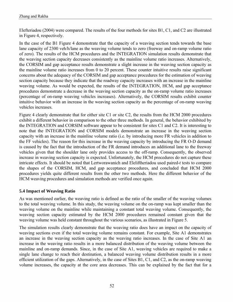
Zhang and Rakha

52

Elefteriadou (2004) were compared. The results of the four methods for sites B1, C1, and C2 are illustrated in Figure 4, respectively.

In the case of the B1 Figure 4 demonstrate that the capacity of a weaving section tends towards the base lane capacity of 2300 veh/h/lane as the weaving volume tends to zero (freeway and on-ramp volume ratio of zero). The results of the HCM procedures and the INTEGRATION simulation results demonstrate that the weaving section capacity decreases consistently as the mainline volume ratio increases. Alternatively, the CORSIM and gap acceptance results demonstrate a slight increase in the weaving section capacity as the mainline volume ratio increases from 0 to 20 percent. These counter intuitive results raise significant concerns about the adequacy of the CORSIM and gap acceptance procedures for the estimation of weaving section capacity because they indicate that the roadway capacity increases with an increase in the mainline weaving volume. As would be expected, the results of the INTEGRATION, HCM, and gap acceptance procedures demonstrate a decrease in the weaving section capacity as the on-ramp volume ratio increases (percentage of on-ramp weaving vehicles increases). Alternatively, the CORSIM results exhibit counter intuitive behavior with an increase in the weaving section capacity as the percentage of on-ramp weaving vehicles increases.

Figure 4 clearly demonstrate that for either site C1 or site C2, the results from the HCM 2000 procedures exhibit a different behavior in comparison to the other three methods. In general, the behavior exhibited by the INTEGRATION and CORSIM software appear to be consistent for sites C1 and C2. It is interesting to note that the INTEGRATION and CORSIM models demonstrate an increase in the weaving section capacity with an increase in the mainline volume ratio (i.e. by introducing more FR vehicles in addition to the FF vehicles). The reason for this increase in the weaving capacity by introducing the FR O-D demand is caused by the fact that the introduction of the FR demand introduces an additional lane to the freeway vehicles given that the shoulder lane only provides access to the off-ramp. Consequently, the observed increase in weaving section capacity is expected. Unfortunately, the HCM procedures do not capture these intricate effects. It should be noted that Lertworawanich and Eleliftheriadou used paired-t tests to compare the shapes of the CORSIM, HCM, and gap acceptance procedures, and concluded that HCM 2000 procedures yields quite different results from the other two methods. Here the different behavior of the HCM weaving procedures and simulation methods are verified once again.

5.4 Impact of Weaving Ratio

As was mentioned earlier, the weaving ratio is defined as the ratio of the smaller of the weaving volumes to the total weaving volume. In this study, the weaving volume on the on-ramp was kept smaller than the weaving volume on the mainline while maintaining a constant total weaving volume. Consequently, the weaving section capacity estimated by the HCM 2000 procedures remained constant given that the weaving volume was held constant throughout the various scenarios, as illustrated in Figure 5.

The simulation results clearly demonstrate that the weaving ratio does have an impact on the capacity of weaving sections even if the total weaving volume remains constant. For example, Site A1 demonstrates an increase in the weaving section capacity as the weaving ratio increases. In the case of Site A1 an increase in the weaving ratio results in a more balanced distribution of the weaving volume between the mainline and on-ramp demands. Since, in the case of Site A1, weaving vehicles are required to make a single lane change to reach their destination, a balanced weaving volume distribution results in a more efficient utilization of the gaps. Alternatively, in the case of Sites B1, C1, and C2, as the on-ramp weaving volume increases, the capacity at the core area decreases. This can be explained by the fact that for a

Zhang and Rakha

53

constant weaving volume, more on-ramp weaving vehicles requires more lane change maneuvers within the weaving section and thus increases the turbulence within the weaving section.

5.5 Impact of Weaving Section Length

The effect of weaving section length on weaving section capacity is a controversial issue that has resulted in significant debate over the past years. The study investigates the impact of weaving section length on the capacity of weaving sections using the INTEGRATION software and the HCM procedures, as demonstrated in Figure 6. The results of the two approaches for the four sites demonstrate significantly differing trends. Specifically, the simulation results, unlike the HCM procedures, demonstrate that the impact of the weaving section length on the capacity of a weaving section increases as the traffic demand increases. Clearly, the simulation results appear to be more intuitive.

It is worthy to note that in Figure 6, the simulation results demonstrate that as the weaving volume increases, the weaving section capacity increases initially and then decreases. After a close look at the geometric layout of Sites C1 and C2 in Figure 1 the simulation results appear to be very reasonable. For example, at Site C1, a freeway volume ratio of zero requires that the freeway-to-freeway (FF) vehicles initially travel through a 3-lane segment followed by a 2-lane segment within the weaving section. Alternatively, the ramp-to-ramp (RR) vehicles initially travel on a single lane followed by a 3-lane segment within the weaving section. Consequently, the FF vehicles, unlike the RR vehicles, encounter a bottleneck within the weaving section. Alternatively, if the FF vehicles switch to FR vehicles, the FR are then able to utilize a number of the off-ramp lanes and thus travel along a wider roadway segment. Noteworthy is the fact that the HCM 2000 procedures indicate that the weaving section capacity decreases as the volume ratio increases, which does not appear to be reasonable.

Based on the converging lines of Figure 6 we can conclude that, in general, as the weaving section length increases, its impact on the weaving section capacity decreases. For example, the decrease in the weaving section capacity resulting from an increase of 150m for a 150m weaving section is significantly different than its impact on a 600m weaving section.

5.6 Impact of Speed Limit Differential between Mainline and Ramps

A number of studies have indicated that the lower speeds of vehicles on on- and off-ramps affect the operation of weaving sections significantly. Consequently, as part of this study the impact of the speed limit differential between freeway and ramps on the capacity of weaving sections is analyzed in a systematic fashion. Specifically, Sites B1, C1, and C2 are analyzed for three weaving intensities are considered, namely low, medium, and high. In the case of Site B1 the three volume ratios that are considered are 10, 40, and 80 percent while in the case of Sites C1 and C2 volume ratios of 5, 25, and 50 percent are considered. These values were selected based on the maximum recommended values for Type B and C weaving sections for the HCM 2000 procedures.

Statistical analysis of the results (average of 30 simulation runs) using the Kruskal-Wallis test for K independent samples revealed that, at a level of significance of 5 percent (α = 0.05), there does not exist enough evidence to conclude that the speed limit differential between the freeway mainline and the on- and off-ramps affects the capacity of freeway weaving sections. The p-values of the test are demonstrated in Table 2. For each cell in the table, a Kruskal-Wallis test is performed with six samples: differentials of 0, 5, 10, 15, 20, 25, and 30 km/h.

Zhang and Rakha

54

5.7 Impact of Heavy Vehicles

In this section the impact of heavy vehicles on the capacity of weaving sections is analyzed using the INTEGRATION software and the HCM procedures, as illustrated in Figure 7. Figure 7 demonstrates a high degree of consistency between the simulation and HCM results for all four sites, although the simulation results tended to be less than the HCM results. Consequently, the results of this sensitivity analysis demonstrate the adequacy of the HCM procedures in capturing the impacts of heavy vehicles on the capacity of weaving sections.

5.8 Differentiation between Type B Configurations

As stated in Section 4, this study investigates whether differences in the capacities of both configurations of Figure 2 warrant considering different configuration types. The two configurations are considered for a weaving length of 600m using an identical O-D demand, with a weaving ratio of 30 percent and an on-ramp volume of 30 percent the total in-coming total demand. The simulation results that are illustrated in Figure 8 demonstrate that the capacity of configuration 1 is typically less than that of configuration 2, especially for high volume ratios. The lower capacity of configuration 1 can be attributed to the fact that freeway-to-ramp (FR) vehicles do not require to execute any lane changes for the second configuration, which is not the case for the first configuration. Consequently, the simulation results verify the suggestion of separating the two configurations into two different weaving section types.

6. FINDINGS AND CONCLUSIONS The research presented in this paper examined one of the most important aspects of analysis of freeway weaving sections, namely the capacity analysis. The findings and conclusions of the study can be summarized as follows:

a. The study demonstrated the validity of the INTEGRATION software for the analysis of weaving section capacities.

b. The study demonstrated some questionable capacity estimates by the CORSIM software and a gap acceptance procedure proposed in the literature. Specifically, the results demonstrated an unrealistic increase in roadway capacity with an increase in the mainline weaving volume for a Type B weaving section.

c. The study demonstrated that the random number seed resulted in a weaving section capacity standard deviation of 65 veh/h/lane.

d. The weaving ratio, which the ratio of the lowest weaving volume to the total weaving volume, has a significant impact on the capacity of weaving sections. Unfortunately, the weaving ratio is not considered in the HCM 2000 procedures.

e. The length of weaving section has a larger impact on the capacity of weaving sections for short lengths and high traffic demands.

f. There does not exist enough evidence to conclude that the speed limit differential between freeway and ramps has a significant impact on weaving section capacities.

g. The HCM procedures for accounting for heavy duty vehicle impacts on weaving section capacities appear to be reasonable.

h. The separation of weaving sections requiring no lane changing by weaving flows should be separated from other Type B weaving sections.

Zhang and Rakha

55

i. Simulation is a very useful tool for the capacity analysis of freeway weaving sections.

ACKNOWLEDGEMENTS The authors would like to acknowledge the financial support of the Mid-Atlantic University Transportation Center (MAUTC) in conducting this research effort.

REFERENCES Bacon, V., et al., Use of INTEGRATION Model to Study High-Occupancy-Vehicle Facilities,

Transportation Research Record No. 1446, 1994, pp. 8-13.

Dion F., Rakha H., and Zhang Y. (In press), Evaluation of Potential Transit Signal Priority Benefits Along a Fixed-Time Signalized Arterial. ASCE Journal of Transportation Engineering.

Gardes, Y. and A.D. May. Simulation of IVHS on the Smart Corridor Using the INTEGRATION Model: Initial Investigation. PATH Research Report, UCB-ITS-PRR-93-3, 1993.

Hellinga, B., and Van Aerde, M., An Overview of a Simulation Study of the Highway 401 Freeway Traffic Management System, Canadian Journal of Civil Engineering, Vol. 21, 1994.

Highway Capacity Manual (HCM) 2000 – Weaving Segments, Chapter 24, Transportation Research Board, National Research Council, Washington, D.C. 2000

Kwon, E., Lau, R., and Aswegan, J., Maximum Possible Weaving Volume for Effective Operations of Ramp-Weave Areas, Transportation Research Record, n 1727, 2000, pp. 132-141.

Lertworawanich, P. and Elefteriadou, L., Capacity Estimations for Type-B Weaving Areas Based on Gap Acceptance, Transportation Research Record 1776, TRB, National Research Council, Washington, D.C. 2002.

Lertworawanich, P. and Elefteriadou, L., Methodology for Estimating Capacity at Ramp Weaves Based on Gap Acceptance and Linear Optimization, Transportation Research B: Methodological Vol. 37, 2003, pp.459-483.

Lertworawanich, P. and Elefteriadou, L., Evaluation of Three Freeway Weaving Capacity Estimation Methods and Comparison to Field Data, Freeway Capacity, TRB 2004 Annual Meeting CD-Rom.

Rakha, H., Van Aerde, M., Bloomberg, L., and X. Huang, Construction and Calibration of a Large-Scale Micro-Simulation Model of the Salt Lake Area, Paper presented at the 77th Transportation Research Board Annual Meeting, Washington, D.C., January 11-15, 1998.

Rakha H., Medina A., Sin H., Dion F., Van Aerde M., and Jenq J., Coordination of Traffic Signals Across Jurisdictional Boundaries: Field and Simulation Results, Transportation Research Board 79th Annual Meeting, Washington DC, January, 2000, CD-ROM [Paper # 00-1560].

Rakha H. and Crowther B. (2003), Comparison and Calibration of FRESIM and INTEGRATION Steady-state Car-following Behavior, Transportation Research, 37A, pp. 1-27.

Rakha H., Pasumarthy P., and Adjerid S. (2004), Car-Following Models: Formulations, Issues, and Practical Considerations, Submitted to the Journal of Transportation Research.

Rakha H. and Ahn K. (2004), The INTEGRATION Modeling Framework for Estimating Mobile Source Emissions. ASCE Journal of Transportation Engineering, March Issue.

Zhang and Rakha

56

Roess, R. and Ulerio, J., Weaving Area Analysis in Year 2000 Highway Capacity Manual, Transportation Research Record, n 1710, 2000, pp. 145-153.

Skabardonis, A., Cassidy, M., May, A. D., and Cohen, S., Application of Simulation To Evaluate the Operation of Major Freeway Weaving Sections, Transportation Research Record, n 1225, 1989, pp. 91-98.

Special Report 209: Highway Capacity Manual. TRB, National Research Council, Washington, D.C., 1985.

Stewart, J. Baker, M. Van Aerde, M. Evaluating Weaving Section Designs Using INTEGRATION, Transportation Research Record, n 1555, 1996, pp. 33-41.

Vermijs, R., New Dutch Capacity Standards for Freeway Weaving Sections Based on Micro Simulation, Third International Symposium on Highway Capacity, 1998, pp. 1065-1080.

Zarean, M. and Nemeth, Z. A., WEASIM: A Microscopic Simulation Model of Freeway Weaving Sections, Transportation Research Record, n 1194, 1988, pp. 48-54.

Zhang and Rakha

57

LIST OF TABLES Table 1: Geometrical and Traffic Factors Table 2: p-values of Kruskal-Wallis Tests of Speed Differentials

LIST OF FIGURES Figure 1: Configurations of Test Weaving Sections Figure 2: Configurations of Alternative Type B Weaving Sections Figure 3: Validation Results for Sites B1, C1, and C2 Figure 4: Capacity Surfaces for Sites B1, C1, and C2 Figure 5: Impact of Weaving Ratio on Capacity Figure 6: Impact of Weaving Section Length on Capacity Figure 7: Impact of Heavy Duty Vehicles on Capacity Figure 8: Capacity of Both Type B Configurations

Zhang and Rakha

58

Table 1: Geometrical and Traffic Factors Parameter Values considered Weaving section type Type A, Type B and Type C Weaving ratio 0.0, 0.1, 0.2, 0.3, 0.4, 0.5 Weaving section length 150, 300, 450, 600, and 750 m Speed limit differential between freeway and on-ramp 0, 5, 10, 15, 20, 25, and 30 km/h Speed limit differential between freeway and off-ramp 0, 5, 10, 15, 20, 25, and 30 km/h Percentage heavy duty vehicles 0, 5, 10, 15, 20, and 25%

Table 2: p-values of Kruskal-Wallis Tests of Speed Limit Differentials B1 C1 C2 On - F Off - F On - F Off - F On - F Off - F H 0.365 0.615 0.944 0.447 0.521 0.120 M 0.066 0.748 0.056 0.305 0.083 0.774 L 0.494 0.956 0.058 0.886 0.097 0.334

On - F: Speed limit differential between on-ramp and freeway Off - F: Speed limit differential between off-ramp and freeway H: high VR conditions (0.80 for site B1 and 0.50 for Sites C1 and C2) M: medium VR conditions (0.40 for site B1 and 0.25 for Sites C1 and C2) L: low VR conditions (0.10 for site B1 and 0.05 for Sites C1 and C2)

Zhang and Rakha

59

300 m

Site A1

550 m

Sites B1

660 m

Site C1

500 m

Sites C2

Figure 1: Configurations of Test Weaving Sections

600 m B

A

D

C

Configuration 1

600 mB

A

D

C

Configuration 2

Figure 2: Configurations of Alternative Type B Weaving Sections

Zhang and Rakha

60

Calibration of Site B1

Calibration of Site C1

Calibration of Site C2

4000

5000

6000

7000

8000

1 2 3 4 5 6 7 8 9 10Date

Cap

acity

(vph

)

FieldINTEGRATION

6000

7000

8000

9000

10000

1 2 3 4 5 6 7 8 9 10Date

Cap

acity

(vph

)

FieldINTEGRATION

5000

6000

7000

8000

9000

1 2 3 4 5 6 7 8 9 10 11 12 13 14 15 16Date

Cap

acity

(vph

)

FieldINTEGRATION

Figure 3: Validation Results for Sites B1, C1, and C2

Zhang and Rakha

61

00.2

0.40.6

0.81

0

0.4

0.8

0250500750

1000125015001750200022502500

Cap

acity

(veh

/h/la

ne)

Freeway VR Ramp VR

B1 - INTEGRATION

00.2

0.40.6

0.81

0

0.4

0.8

0250500750

100012501500175020002250

Freeway VR Ramp VR

B1 - CORSIM

00.2

0.40.6

0.81

0

0.4

0.8

0250500750

100012501500175020002250

Freeway VR Ramp VR

B1 - HCM 2000

00.2

0.40.6

0.81

0

0.4

0.8

0250500750

100012501500175020002250

Freeway VR Ramp VR

B1 - Gap Acceptance Method

2000-22501750-20001500-17501250-15001000-1250750-1000500-750250-5000-250

00.2

0.40.6

0.81

0

0.4

0.8

0250500750

10001250150017502000

Cap

acity

(veh

/h/la

ne)

Freeway VR Ramp VR

C1 - INTEGRATION

00.2

0.40.6

0.81

0

0.4

0.8

0250500750

10001250150017502000

Freeway VR Ramp VR

C1 - CORSIM

00.2

0.40.6

0.81

0

0.4

0.8

0250500750

10001250150017502000

Freeway VR Ramp VR

C1 - HCM 2000

00.2

0.40.6

0.81

0

0.4

0.8

0250500750

100012501500

1750

2000

Freeway VR Ramp VR

C1 - Gap Acceptance Method

1750-20001500-17501250-15001000-1250750-1000500-750250-5000-250

00.2

0.40.6

0.81

0

0.4

0.8

0250500750

10001250150017502000

Cap

acity

(veh

/h/la

ne)

Freeway VR Ramp VR

C2 - INTEGRATION

00.2

0.40.6

0.81

0

0.4

0.8

0250500750

100012501500175020002250

Freeway VR Ramp VR

C2 - CORSIM

00.2

0.40.6

0.81

0

0.4

0.8

0250500750

100012501500175020002250

Freeway VR Ramp VR

C2 - HCM 2000

00.2

0.40.6

0.81

0

0.4

0.8

0250500750

100012501500175020002250

Freeway VR Ramp VR

C2 - Gap Acceptance Method

2000-22501750-20001500-17501250-15001000-1250750-1000500-750250-5000-250

Figure 4: Capacity Surfaces for Sites B1, C1, and C2

Zhang and Rakha

62

4000

6000

8000

0.0 0.1 0.2 0.3 0.4 0.5Weaving Ratio

Cap

acity

(veh

/h)

A1 - HCMA1 - INTEGRATION

4000

6000

8000

0.0 0.1 0.2 0.3 0.4 0.5Weaving Ratio

Cap

acity

(veh

/h)

B1 - HCMB1 - INTEGRATION

8000

10000

12000

0.0 0.1 0.2 0.3 0.4 0.5Weaving Ratio

Cap

acity

(veh

/h) C1 - HCM

C1 - INTEGRATION

5000

7000

9000

0.0 0.1 0.2 0.3 0.4 0.5Weaving Ratio

Cap

acity

(veh

/h)

C2 - HCMC2 - INTEGRATION

Figure 5: Impact of Weaving Ratio on Capacity

Zhang and Rakha

63

5000

6000

7000

8000

9000

10000

0.1 0.15 0.2 0.25 0.3 0.35Volume Ratio

INTE

GR

ATI

ON

Cap

. (vp

h)

150 m300 m450 m600 m750 m

5000

6000

7000

8000

9000

10000

0.1 0.15 0.2 0.25 0.3 0.35Volume Ratio

HC

M C

apac

ity (v

ph)

150 m300 m450 m600 m750 m

Site A1

3000

4000

5000

6000

7000

8000

9000

0.1 0.2 0.3 0.4 0.5 0.6 0.7 0.8

Volume Ratio

INTE

GR

ATI

ON

Cap

.(vph

)

150 m300 m450 m600 m750 m

3000

4000

5000

6000

7000

8000

9000

0.1 0.2 0.3 0.4 0.5 0.6 0.7 0.8

Volume Ratio

HC

M C

apac

ity (v

ph)

150 m300 m450 m600 m750 m

Site B1

6000

7000

8000

9000

10000

11000

0.1 0.2 0.3 0.4 0.5Volume Ratio

INTE

GR

ATI

ON

Cap

.(vph

)

150 m300 m450 m600 m750 m 6000

7000

8000

9000

10000

11000

0.1 0.2 0.3 0.4 0.5

Volume Ratio

HC

M C

apac

ity (v

ph)

150 m300 m450 m600 m750 m

Site C1

5000

6000

7000

8000

9000

0.1 0.2 0.3 0.4 0.5Volume Ratio

INTE

GR

ATI

ON

Cap

. (v

ph)

150 m300 m450 m600 m750 m

5000

6000

7000

8000

9000

0.1 0.2 0.3 0.4 0.5Volume Ratio

HC

M C

apac

ity (v

ph)

150 m300 m450 m600 m750 m

Site C2

Figure 6: Impact of Weaving Section Length on Capacity

Zhang and Rakha

64

4000

5000

6000

7000

8000

9000

0 0.05 0.1 0.15 0.2 0.25Heavy Vehicle Rate

Cap

acity

(vph

) Site A1 - HCMSite A1 - INTEGRATION

400050006000700080009000

10000

0 0.05 0.1 0.15 0.2 0.25Heavy Vehicle Rate

Cap

acity

(vph

) Site B1 - HCMSite B1 - INTEGRATION

6000

7000

8000

9000

10000

11000

0 0.05 0.1 0.15 0.2 0.25Heavy Vehicle Rate

Cap

acity

(vph

) Site C1 - HCMSite C1 - INTEGRATION

3000400050006000700080009000

0 0.05 0.1 0.15 0.2 0.25Heavy Vehicle Rate

Cap

acity

(vph

) Site C2 - HCMSite C2 - INTEGRATION

Figure 7: Impact of Heavy Duty Vehicles on Capacity

Zhang and Rakha

65

0

1000

2000

3000

4000

5000

6000

0 0.05 0.1 0.15 0.2 0.25 0.3 0.35 0.4

Volume Ratio

Sim

ulat

ed C

apac

ity(v

eh/h

)

1

2

Figure 8: Capacity of Both Type B Configurations

66

Chapter 5. Analytical Procedures for Estimating Capacity of Type B Weaving Sections

(Transportation Research Board annual meeting 2005, paper# 05-2483)

67

Analytical Procedures for Estimating Capacity of Type B Weaving Sections

Hesham Rakha1 and Yihua Zhang2

Word count: 5,119 Tables and figures: 2,250 Total word count: 7,369

ABSTRACT The paper identifies thirteen common configurations of Type B weaving sections. These configurations are modeled using the INTEGRATION software for a wide range of weaving section lengths and travel demands. Subsequently, the simulation results are utilized to develop analytical procedures for estimating the capacity of Type B weaving sections and compared to the HCM2000 procedures. The results demonstrate that the HCM2000 procedures suffer from four significant drawbacks. First, the procedures can only consider relatively long weaving sections (longer than or equal to 150 m). Second, the HCM procedures fail to capture the impact of the distribution of weaving flows between freeway and on-ramp demand on the capacity of weaving sections, which is demonstrated to be an important factor in the analysis weaving section capacities. Third, the procedures do not ensure that the capacity of a weaving section reverts to the basic freeway capacity when the volume ratio is zero (no weaving flows) regardless of the weaving section length. Finally, the HCM procedures do not ensure consistency between the weaving and merge/diverge procedures at the boundary conditions. The paper demonstrates that the proposed analytical model overcomes the four identified shortcomings of the HCM2000 procedures and estimates the capacity of weaving sections to within 14 percent of the simulated results compared to the HCM error of 151 percent.

Key words: Freeway weaving sections, capacity of freeway weaving sections, freeway capacity modeling, HCM 2000, and INTEGRATION software.

INTRODUCTION The freeway weaving analysis procedures in the 2000 Highway Capacity Manual (1) are based on research conducted in the early 1970s through the early 1980s (2). Subsequent research efforts have shown that the methods’ ability to predict the operation of a weaving section is limited (3, 4, 5), which is most probably due to the outdated and limited database that was utilized to develop these models. As to capacity estimation of freeway weaving sections, some other methods such as gap-acceptance and simulation methods have been used as alternatives (3, 4, 6, 7).

1 Charles Via Jr. Department of Civil and Environmental Engineering, Virginia Tech, 3500 Transportation Research Plaza (0536), Blacksburg, VA 24061. E-mail: hrakha@vt.edu. 2 Charles Via Jr. Department of Civil and Environmental Engineering, Virginia Tech, E-mail: yizhang@vt.edu.

Rakha and Zhang

68

In this paper the INTEGRATION software is utilized to estimate the capacity of weaving sections. The validity of the INTEGRATION software for modeling weaving sections and estimating the capacity of these sections is described in detail in the literature (5, 8), and will be summarized later in the paper. Using a wide spectrum of simulation results, a new analytical model for estimating the capacity of weaving sections is developed. Initially, the paper identifies the sub-types and major configurations within Type B weaving sections. Subsequently, a wide range of weaving section traffic demands is modeled using the INTEGRATION software for all identified major configurations. Specifically, a sensitivity analysis is conducted considering different weaving section lengths and different traffic demands. Subsequently, an analytical capacity model is developed for each configuration.

This paper initially describes the INTEGRATION framework for modeling weaving sections and the validity of this simulation tool for modeling weaving sections. Subsequently, the state-of-the-art studies on the capacity of weaving sections are presented followed by a description of the field data that were utilized to validate the INTEGRATION capacity modeling procedures. Subsequently, the identified common configurations within Type B weaving sections are introduced and the related characteristics of these configurations are described. Subsequently, the simulated capacity estimates are compared to the HCM procedure estimates. Afterwards, an analytical model for estimating Type B weaving sections is presented and compared to the simulation results and the HCM2000 procedures. Finally the findings and conclusions of the study are presented.

INTEGRATION FRAMEWORK FOR MODELING WEAVING SECTIONS The INTEGRATION software is a microscopic traffic simulation and assignment model that can represent traffic dynamics in an integrated freeway and traffic signal network. The model has been successfully applied since the early 1990's in North America and Europe (9, 10, 11, 12, 13, 14, 15). The INTEGRATION 2.30 lane-changing logic was described and validated against field data in an earlier publication (5). Furthermore, Zhang and Rakha (8) demonstrated the validity of the INTEGRATION software for estimating the capacity of weaving sections by comparing to field observed weaving section capacities. A brief description of these studies is presented in this section.

Rakha and Zhang (5) utilized an empirical data set that was gathered in the late 1980's by the University of California at Berkeley (16). In this dataset vehicle spatial distributions both total and by movement, at successive reference points on nine weaving sites were gathered. The traffic movements included the four possible Origin-Destination (O-D) demands on freeway weaving sections, namely, Freeway-to-Freeway (FF), Freeway-to-Ramp (FR), Ramp-to-Freeway (RF), and Ramp-to-Ramp (RR). The volume counts were provided at 5-min intervals at a few reference points along the core weaving area. Using these data the study demonstrated that the lane changing behavior within a weaving section is a very complicated phenomenon that is affected by many factors including the geometric configuration of the weaving section, the O-D demand, and any upstream and downstream routing constraints. Rakha and Zhang demonstrated a high level of consistency between the INTEGRATION software and field data in the spatial and temporal distribution of lane-change intensity across the weaving lanes that fell within the margin of daily variability (i.e. a margin of error of 250 veh/h). Consequently, the study concluded that the INTEGRATION software was appropriate for the modeling of weaving sections.

Rakha and Zhang

69

Zhang and Rakha (8) validated the INTEGRATION software weaving section capacity estimates by comparing to field observed capacities. The study concluded that the capacity estimates of the INTEGRATION software were consistent with field data both in terms of magnitude and trends (mean average relative error less than 5 percent). Furthermore, the results demonstrated that the INTEGRATION capacity estimates were superior to the CORSIM and gap acceptance estimates when compared to field data. In addition, the study demonstrated that the weaving ratio, which is the ratio of the lowest weaving volume to the total weaving volume, has a significant impact on the capacity of weaving sections. Unfortunately, the weaving ratio is not considered in the HCM 2000 capacity procedures. Furthermore, the study demonstrated that the length of weaving section has a larger impact on the capacity of weaving sections as the length of the weaving section decreases and the traffic demand increases. The study also demonstrated that there is no evidence to conclude that the speed differential between the freeway and ramp traffic has a significant impact on weaving section capacities. The study demonstrated that the HCM procedures for accounting for heavy duty vehicle impacts on weaving section capacities are reasonable.

STATE-OF-THE-ART WEAVING ANALYSIS PROCEDURES A limited number of publications were found in the literature that was deemed related to this study. For example, Zarean and Nemeth (17) utilized the WEAVSIM microscopic simulation model, to investigate the effect of different arrival speeds on the operation of weaving sections. Subsequently, the researchers developed a regression model for the modeling of weaving sections based on the simulation results. The simulation results demonstrated that the speed differential between the mainline and on-ramp arrivals had a significant effect on the operation of weaving sections, which was not considered in the 1985 HCM procedures (18) and is not considered in the current HCM procedures (1). However, Zhang and Rakha (8) demonstrate that the speed differential between freeway and ramps has a minimal impact on the capacity of weaving sections.

Skabardonis et al. (19) applied the INTRAS microscopic simulation model to evaluate the operation of a few major freeway weaving sections. INTRAS was modified to predict the speeds of weaving and non-weaving vehicles and was applied to eight major freeway weaving sections. Vehicle speeds within the weaving sections were compared to a few analytical procedures that included the 1985 HCM procedure, Leisch’s procedure, JHK’s procedure, Fazio’s Procedure, and the Polytechnic Institute of New York (PINY) procedure. The researchers concluded that the INTRAS speed predictions were closer to the field measurements than the analytical procedure speed predictions. The researchers concluded that simulation tools could be utilized with field data to enhance existing state-of-the-art analytical procedures for the modeling of weaving section operations.

Stewart et al. (6) evaluated the capability of INTEGRATION version 1.50 for the modeling of weaving sections. The study showed that both the 1985 HCM procedure and INTEGRATION offered identical conclusions for a given sample problem. However, the study demonstrated differences between the two approaches on critical design parameters of weaving sections. Specifically INTEGRATION identified the number of lanes in the core area as a critical factor that affects the capacity of weaving sections, which was not, and continues to not be, captured in the HCM procedures. Alternatively, while the HCM procedures demonstrated that the length of the core area was critical in the design of weaving sections, the INTEGRATION results demonstrated

Rakha and Zhang

70

that this factor was critical for short lengths but was less critical as the weaving section length increased.

Vermijs (20) reported on the efforts in developing the Dutch capacity standards for freeway weaving sections using FOSIM (Freeway Operations SIMulation), a microscopic simulation software developed in the Netherlands. Specifically, a total of 315 Type A weaving sections with different configurations and traffic factors were simulated. All simulation runs were repeated 100 times using different random seeds. The 100 simulation results for capacity appeared to be normally distributed with standard deviation in the range of 200 ~ 400 veh/h/lane.

Finally, Lertworawanich and Elefteriadou (3, 21) proposed an analytical capacity estimation method for weaving sections based on gap acceptance and linear optimization techniques. It should be noted, however that the gap acceptance method makes a number of simplifying assumptions that limit the applicability of the procedures. For example, the procedures are insensitive to the effect of the weaving section length on the capacity of weaving sections.

EXPERIMENTAL DESIGN According to the HCM 2000 procedures, the unique lane changing requirements that characterize Type B weaving sections include a weaving movement that does not require any lane changes and the weaving movement that requires at most a single lane change. In this study, three sub-types of Type B weaving sections are considered (Bx, By and Bz). Sub-type Bx weaving sections require only one lane change for the FR movement and no lane changes for the RF movement, while sub-type By weaving sections involve no required lane changes at the entry gore with a required lane change at the exit gore due to an imbalance in the exit versus entry lanes. Alternatively, Sub-type Bz weaving sections require no lane changes at the entrance and exit gores (lane balance between entry and exit sections). Because Type B weaving sections typically have three, four, or five lanes in the core area, a total of 13 configurations are investigated, as shown in Figure 1.

In terms of the simulation runs, the input free-flow speed along the freeway was set at 110 km/h (68.75 mi/h), while the free-flow speed on the ramps was set at 90 km/h (56 mi/h) if the ramp was a single lane otherwise the ramp free-flow speed was set at 110 km/h. No heavy vehicles were considered as part of the analysis because Zhang and Rakha (8) demonstrated that the heavy vehicle factor within the HCM 2000 procedures efficiently captures the effects of heavy vehicles on the capacity of weaving sections and thus does not require further enhancement. The lane capacity was set at 2,350 and 2,000 veh/h/lane for facilities with free-flow speeds of 110 km/h and 90 km/h, respectively, which is consistent with the HCM 2000 procedures. The speed-at-capacity was set at 80 percent the free-speed, which has been demonstrated to be the norm on North American freeways (22).

The first step in this study was to simulate all thirteen configurations in INTEGRATION considering different weaving section lengths and different Origin-Destination (O-D) demands. Weaving section lengths of 50, 75, 100, 150, 300, 450, 600, and 750 meters were considered in the study, which covers the maximum range of the HCM 2000 procedures in addition to covering lengths shorter than what is considered in the HCM procedures. Different O-D patterns were considered by changing the mix of FF, FR, RF, and RR demands. An attempt was made to cover the entire possible range of O-D demands including the extreme conditions when the weaving section converges to a basic freeway section, a merge section, or a diverge section. The coverage of

Rakha and Zhang

71

these extreme conditions ensures that the modeling of weaving section capacity is consistent with the modeling of basic freeway, merge, and diverge sections because these scenarios represent a special case of a weaving section O-D demand. Specifically, a merge scenario only includes FF and RF demands while a diverge scenario only includes FF and FR demands.

SIMULATION RESULTS AND PROPOSED MODEL This section presents the simulation results and corresponding HCM results. It should be noted that the HCM 2000 does not include any analytical procedures for estimating the capacity of weaving sections. Instead, the procedures provide lookup tables for estimating the capacity of weaving sections. Consequently, there is a need to develop some form of analytical procedures that are capable of estimating the capacity of weaving sections. Furthermore, because of the observed differences between the simulation results and HCM procedures, a refined capacity model is desired.

As was stated earlier, for each configuration, a wide variety of traffic conditions and core weaving area lengths are simulated using the INTEGRATION software. The simulated capacities are estimated as the maximum 15-minute flow rate that proceeds through a weaving section by systematically increasing the O-D demand. Alternatively, the HCM capacities are calculated according to the capacity tables (Exhibit 24-8) in Chapter 24 of the HCM 2000 using interpolation. Since the HCM 2000 procedures do not cover weaving section lengths of 50, 75, and 100 meters and only consider a maximum volume ratio of 80 percent, the simulation scenarios go beyond the confines of the HCM procedures.

In order to generalize the results of this study to consider differing basic freeway section and ramp capacities, a capacity factor is computed. The normalized capacity factor is computed as the maximum section throughput divided by the capacity of the roadway section directly upstream of the weaving section (sum of upstream freeway and on-ramp capacities). For example, the capacity directly upstream of the weaving section for configuration Bx1 is 9,400 veh/h (2×2,350 + 2×2,350). It should be noted that a factor of 1.0 reflects a maximum throughput that is equal to the capacity of the entry section. The capacity of a weaving section can be computed as the product of the reduction factor with the capacity of the entry feeds to the weaving section. It should be noted that in some instances the capacity of the weaving section is governed by the capacity of the outbound roadways, as opposed to the inbound roadways, and thus the reduction factor would not necessarily equal to 1.0 when the volume ratio is set to zero (sum of RF and FR volumes equals 0).

Comparison between Simulated and HCM Capacity Estimates

For ease of comparison, the capacities derived from the HCM procedures are also normalized in the same fashion as was described earlier. Due to space limitation, only the results for configurations Bx1, By1, and Bz1, for lengths of 100, 300, and 600 meters are illustrated in Figure 2 through Figure 4. The figures clearly demonstrate that the differences between the simulated and HCM capacity estimates are significant in both absolute values and trends. For example, the HCM procedures demonstrate that the volume ratio has no impact on the weaving section capacity for small volume ratios. Furthermore, the HCM procedures indicate that the effect of the volume ratio on the weaving section capacity decreases as the weaving length increases. These trends, however, were not observed in the simulation results. Furthermore, the simulated capacity estimates

Rakha and Zhang

72

demonstrate a zigzag pattern that may appear as noise in the data at first glance; however, these oscillations reflect the impact of other factors on the weaving section capacity including the weaving ratio (ratio of weaving volume to the total arrival volume). Zhang and Rakha (8) have demonstrated that the weaving ratio does have a significant impact on the capacity of freeway weaving sections.

The figures also clearly demonstrate that the HCM capacity estimates are significantly higher than the simulated capacity estimates. Given that the INTEGRATION weaving section estimates have been demonstrated to be consistent with field data (8) it is fair to conclude that the HCM procedures tend to over-estimate the capacity of weaving sections.

Proposed Weaving Section Capacity Model

From the above analysis it is obvious that an analytical procedure is required to estimate the capacity of weaving sections. As part of this study a simplistic mathematical function is developed to estimate the capacity of weaving sections. In understanding the relationship between the capacity factor and the various influencing factors including the volume ratio, weaving ratio, and weaving section length each factor was analyzed separately.

While the model structure was the same for all 13 configurations, configuration Bx2 is used to illustrate the model development process. Firstly, the relationship between volume ratio and capacity factor is investigated. For configuration Bx2, this relationship is plotted for each weaving section length. The upper side of Figure 5 illustrates the relationship for all the simulation results of configuration Bx2 for a weaving section length of 100 meters. The figure demonstrates that an exponentially decaying relationship appears to be characteristic of the general behavior (negative exponential function). The structure of the relationship is provided in Equation 1. Similar trends were observed for the other weaving section lengths. Since the maximum value of capacity factor for this configuration is 1.0 (weaving section inbound roadways have a lower capacity than the outbound roadways), the value of the constant a is set to 1.0.

VRteF ⋅⋅= a [1]

In Equation 1 F is the capacity factor, VR is the volume ratio, and a and t are model coefficients that are calibrated. The coefficient of determination was reasonable (78 percent), however as will be discussed later, the model is enhanced by considering other factors in the analysis.

Subsequently, having established the relationship between VR and F, the relationship between the constant t in Equation 1 and the weaving section length (x) was investigated. As shown in the lower side of Figure 5, the relationship between t and x can be modeled as a logarithmic function as

cxbt += ln . [2]

Where b and c are model coefficients and x is the weaving section length in units of meters. It should be noted that the coefficient of determination was extremely high (R2 ≥ 0.95) and all constants were statistically significant.

Combining Equations 1 and 2, the relationship between the F, VR, and x can be expressed as ( ln )b x c VR b VR c VRF a e a x e+ ⋅ ⋅= ⋅ = ⋅ . [3]

Rakha and Zhang

73

It should be noted that given the typical values of the b and c coefficients and the fact that we take the natural logarithm of the weaving section length, the exponent is always negative and thus the relationship ensures that an exponential decay function is established.

Finally, in order to consider the impact of the weaving ratio on the capacity of weaving sections a further analysis of the data was conducted. It should be noted that the HCM 2000 defines the weaving ratio as the ratio of the smaller of the two weaving flows to the total weaving flow. This definition does not distinguish between the FR and RF weaving flows. For example, there are two possible situations for a weaving ratio of 0.30. One possibility is that the FR demand constitutes 30 percent of the total weaving volume or alternatively that the RF demand constitutes 30 percent of the total weaving flow. An analysis of the simulation results revealed significant capacity estimates depending on the source of the weaving volume (FR or RF). In other words the weaving ratio distribution is asymmetric. Consequently, we introduce a new definition of the weaving ratio ( FWR ) as

( )RFFRFRWRF += . [4]

In this model three ranges of WRF are identified. Two threshold values s1 and s2 (where s1 < s2) are identified to establish three regimes. When WRF is less than s1, the majority of the weaving volume is on-ramp to freeway traffic (i.e. predominantly merge traffic). Alternatively, when WRF is greater than or equal to s1 but less than s2, there is a more balanced distribution of the weaving volumes. Finally, when WRF is greater than or equal to s2, the majority of the weaving volume is from freeway to off-ramp (i.e. predominantly diverge traffic). In order to account for differences in behavior as a function of the weaving volume composition, the simulation results are categorized into three categories according to the value of freeway weaving ratio (WRF ≤ s1, s1 < WRF < s2, WRF ≥ s2). The breakpoints s1 and s2 were computed by minimizing the sum of squared error between the estimated and simulated capacity factor estimates as

( )3 2( ln )

1Min Z r rb x c VR

r simr

a e F+

=

= ⋅ −∑∑ . [5]

It should be noted that Equation 5 computes the total error relative to the simulated capacity factor (Fsim) over all observations within each of the three regimes (r = 1,2, and 3). Consequently, the model coefficients of Equation 5 are regime-specific (i.e. the coefficients have a subscript r as ar, br, and cr).

The proposed capacity models for all the identified 13 configurations are summarized in Table 1. It should be noted that the model always reverts to the basic capacity when VR is set to zero. Given that the overall capacity is governed by the lowest capacity bottleneck within the system the constant over the three sections, namely the inbound lanes, the weaving lanes, and the outbound lanes. In the cases that the capacity is constrained by the inbound lanes the coefficient (a) is equal to 1.0, as in the case of scenarios Bx1, Bx2, and Bx3.

Reanalyzing Figure 2 through Figure 4 demonstrates that by incorporating the weaving ratio as a variable within the proposed model, the model is able to capture the majority of oscillations that are observed in the simulated data. Furthermore, these oscillations are demonstrated to not be a result of a random process; instead they reflect the impact of other factors that are significant and not considered in the current HCM procedures.

Rakha and Zhang

74

Significance of Coefficients

To eliminate the redundant dummy items from the proposed model, the 95% confidence intervals of all the coefficients are studied. The confidence intervals are shown in Table 3, with all the intervals including 0 shaded.

Intervals that include 0 mean that the corresponding item in the model is not significant. For example, in Table 3 for configuration Bz2, Bz3, and Bz4 the 95% confidence intervals for coefficient b for diverge condition include 0, which means that in the proposed model, weaving section length is not important for diverge condition for these three configurations. However, to keep consistency of format of the model with other configurations and traffic conditions, this item is always kept in the model.

Proposed Capacity Model Validation

In order to quantify the differences between the simulated capacity estimates and the various analytical model estimates the models were compared for all the scenarios. Four error measures were estimated for each of the data sets. These error measures are the mean relative error (MeRE), the maximum relative error (MaRE), the mean absolute error (MeAE), and the maximum absolute error (MaAE). The errors were derived as

( ) nyyyMeREn

iSBABA ∑

=− −=

1

,

( )SBABA yyyMaRE −=− max ,

( ) nyyMeAEn

iBABA ∑

=− −=

1

, and

( )BABA yyMaAE −=− max . Where ys is the simulated capacity factor, yA and yB represent the capacity factor estimates for the two scenarios being compared (potential scenarios include simulation, HCM, and proposed model), and n is the number of observations analyzed for each scenario.

The results demonstrate that the difference between the proposed model and simulated capacity factors is the smallest among the three comparisons, as illustrated in Table 2. Specifically, the mean absolute error does not exceed 0.04 and the mean relative error is less than 14 percent for all thirteen configurations. However, it should be noted that the maximum absolute error is 0.28 and the maximum relative error for configuration is 106 percent (configuration By2). The error estimates, however, are significantly lower than the current HCM procedures and thus the proposed models offer significant improvements to the current state-of-the-art procedures.

Sensitivity Analysis

A simple sensitivity study is conducted on both the proposed model and the HCM procedures. The conducted study covers different weaving section lengths and volume ratios, and three levels of weaving ratio, which corresponds to the previously mentioned three regimes separated by the threshold values s1 and s2. In Figure 6, the left side shows the sensitivity study results from the proposed model, and on the right side are the results from HCM procedures.

Rakha and Zhang

75

Since HCM procedures do not take weaving ratio into account, In Figure 6 the results for the three levels of weaving ratio are just the same. It seems only that in HCM weaving section length impacts the capacity factor only at a range of volume ratio. As to the proposed model, from the spacing between neighboring curves it shows that volume ratio affects capacity factor more when it is low. And generally as weaving section length gets longer, the impact of weaving section length decreases. Also you will find that except at VR of 0, higher weaving ratio means lower capacity factor when comparing the left three plots. This is reasonable since for configuration Bx2 higher weaving ratio means more lane changes, thus more turbulence to the traffic flow.

FINDINGS AND CONCLUSIONS The research presented in this paper examined one of the most important aspects of analysis of freeway weaving sections, namely the capacity analysis. In this paper the capacity of Type B weaving sections was evaluated using simulation. The simulation results demonstrated that the HCM procedures are not only inadequate but fail to capture critical variables that impact the capacity of weaving sections including the weaving ratio and the distribution of weaving volume between freeway to off-ramp and on-ramp to freeway demands.

The paper presents a very simple analytical model for estimating the capacity of Type B weaving sections. The model includes three independent input variables: the weaving section length, the weaving section volume ratio, and a newly defined variable called the freeway weaving ratio (WRF = FR/(FR+RF)). Specifically, the paper introduces a new definition for the weaving ratio that explicitly accounts for the source of the weaving volume. The paper demonstrates that the proposed analytical model estimates the capacity to within 14 percent of the simulated data. Alternatively, the HCM procedures exhibit errors in the range of 151 percent. The procedures that are developed in this study ensure a number of critical issues. First, the capacity of a weaving section reverts to the bottleneck capacity if the weaving volume ratio is set to zero irrespective of the length of the weaving section. Second, the weaving section capacity reverts to a merge section capacity when WRF is low. Similarly, the weaving section capacity reverts to a diverge section capacity when the WRF is high.

ACKNOWLEDGEMENTS The authors acknowledge the financial support of the Mid-Atlantic University Transportation Center (MAUTC) in conducting this research effort.

REFERENCES 1. Highway Capacity Manual (HCM) 2000 – Weaving Segments, Chapter 24, Transportation

Research Board, National Research Council, Washington, D.C. 2000

2. Roess, R. and Ulerio, J., Weaving Area Analysis in Year 2000 Highway Capacity Manual, Transportation Research Record, n 1710, 2000, pp. 145-153.

3. Lertworawanich, P. and Elefteriadou, L., Capacity Estimations for Type-B Weaving Areas Based on Gap Acceptance, Transportation Research Record 1776, TRB, National Research Council, Washington, D.C. 2002.

Rakha and Zhang

76

4. Lertworawanich, P. and Elefteriadou, L., Evaluation of Three Freeway Weaving Capacity Estimation Methods and Comparison to Field Data, Freeway Capacity, TRB 2004 Annual Meeting CD-Rom.

5. Rakha H. and Zhang Y. (2004), The INTEGRATION 2.30 Framework for Modeling Lane-Changing Behavior in Weaving Sections, TRB, 2004, paper # 04-3422.

6. Stewart, J. Baker, M. Van Aerde, M. Evaluating Weaving Section Designs Using INTEGRATION, Transportation Research Record, n 1555, 1996, pp. 33-41.

7. Kwon, E., Lau, R., and Aswegan, J., Maximum Possible Weaving Volume for Effective Operations of Ramp-Weave Areas, Transportation Research Record, n 1727, 2000, pp. 132-141.

8. Zhang Y. and Rakha H. (2005), Systematic Analysis of Capacity of Weaving Sections, Accepted for presentation at the 84th Transportation Research Board Meeting, Washington DC.

9. Gardes, Y. and A.D. May. Simulation of IVHS on the Smart Corridor Using the INTEGRATION Model: Initial Investigation. PATH Research Report, UCB-ITS-PRR-93-3, 1993.

10. Bacon, V., et al., Use of INTEGRATION Model to Study High-Occupancy-Vehicle Facilities, Transportation Research Record No. 1446, 1994, pp. 8-13.

11. Hellinga, B., and Van Aerde, M., An Overview of a Simulation Study of the Highway 401 Freeway Traffic Management System, Canadian Journal of Civil Engineering, Vol. 21, 1994.

12. Rakha, H., Van Aerde, M., Bloomberg, L., and X. Huang, Construction and Calibration of a Large-Scale Micro-Simulation Model of the Salt Lake Area, Paper presented at the 77th Transportation Research Board Annual Meeting, Washington, D.C., January 11-15, 1998.

13. Rakha H., Medina A., Sin H., Dion F., Van Aerde M., and Jenq J., Coordination of Traffic Signals across Jurisdictional Boundaries: Field and Simulation Results, Transportation Research Board 79th Annual Meeting, Washington DC, January, 2000, CD-ROM [Paper # 00-1560].

14. Rakha H. and Ahn K. (2004), The INTEGRATION Modeling Framework for Estimating Mobile Source Emissions. ASCE Journal of Transportation Engineering, March Issue.

15. Dion F., Rakha H., and Zhang Y. (In press), Evaluation of Potential Transit Signal Priority Benefits along a Fixed-Time Signalized Arterial. ASCE Journal of Transportation Engineering.

16. Cassidy, M., Chan, P., Robinson, B., and A. D. May, A Proposed Analytical Technique for the Design and Analysis of Major Freeway Weaving Sections, Institute of Transportation Studies, University of California-Berkeley, research Report UCB-ITS-RR-90-16. 1990.

17. Zarean, M. and Nemeth, Z. A., WEASIM: A Microscopic Simulation Model of Freeway Weaving Sections, Transportation Research Record, n 1194, 1988, pp. 48-54.

18. Special Report 209: Highway Capacity Manual. TRB, National Research Council, Washington, D.C., 1985.

Rakha and Zhang

77

19. Skabardonis, A., Cassidy, M., May, A. D., and Cohen, S., Application of Simulation to Evaluate the Operation of Major Freeway Weaving Sections, Transportation Research Record, n 1225, 1989, pp. 91-98.

20. Vermijs, R., New Dutch Capacity Standards for Freeway Weaving Sections Based on Micro Simulation, Third International Symposium on Highway Capacity, 1998, pp. 1065-1080.

21. Lertworawanich, P. and Elefteriadou, L., Methodology for Estimating Capacity at Ramp Weaves Based on Gap Acceptance and Linear Optimization, Transportation Research B: Methodological Vol. 37, 2003, pp.459-483.

22. Rakha H. and Van Aerde M., Statistical Analysis of Day-to-Day Variations in Real-Time Traffic Flow Data, Transportation Research Record, No. 1510, pp. 26-34, 1995.

Rakha and Zhang

78

LIST OF TABLES Table 1: Proposed Capacity Model for Type B Weaving Sections Table 2: Differences among Simulated Capacity, HCM Capacity, and Model Capacity Table 3: 95% Confidence Intervals for Exponential Model Coefficients

LIST OF FIGURES Figure 1: Configurations of Type B Weaving Sections Figure 2: Configuration Bx1 Weaving Sections Figure 3: Configuration By1 Weaving Sections Figure 4: Configuration Bz1 Weaving Sections Figure 5: Illustration of Model Development Figure 6: Sensitivity Study Results from the Proposed Model and HCM Procedures for Configuration Bx2

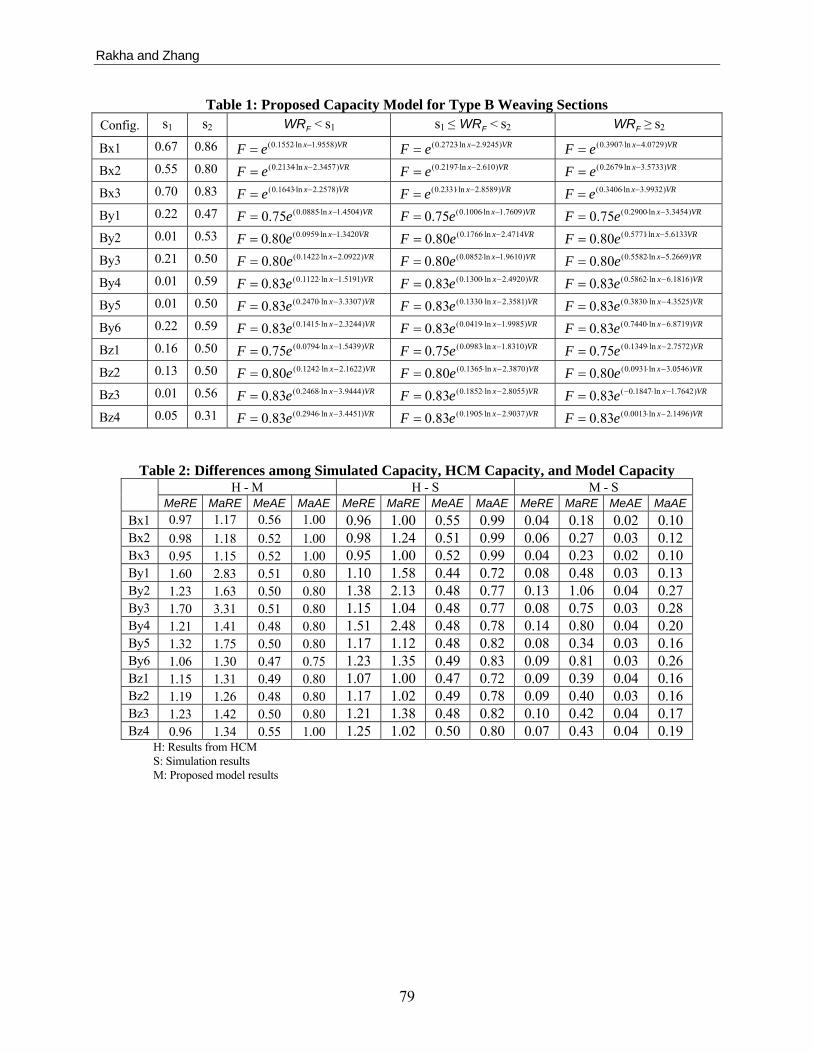
Rakha and Zhang

79

Table 1: Proposed Capacity Model for Type B Weaving Sections Config. s1 s2 FWR < s1 s1 ≤ FWR < s2 FWR ≥ s2

Bx1 0.67 0.86 VRxeF )9558.1ln1552.0( −⋅= VRxeF )9245.2ln2723.0( −⋅= VRxeF )0729.4ln3907.0( −⋅= Bx2 0.55 0.80 VRxeF )3457.2ln2134.0( −⋅= VRxeF )610.2ln2197.0( −⋅= VRxeF )5733.3ln2679.0( −⋅= Bx3 0.70 0.83 VRxeF )2578.2ln1643.0( −⋅= VRxeF )8589.2ln2331.0( −⋅= VRxeF )9932.3ln3406.0( −⋅= By1 0.22 0.47 VRxeF )4504.1ln0885.0(75.0 −⋅= VRxeF )7609.1ln1006.0(75.0 −⋅= VRxeF )3454.3ln2900.0(75.0 −⋅= By2 0.01 0.53 VRxeF 3420.1ln0959.0(80.0 −⋅= VRxeF 4714.2ln1766.0(80.0 −⋅= VRxeF 6133.5ln5771.0(80.0 −⋅= By3 0.21 0.50 VRxeF )0922.2ln1422.0(80.0 −⋅= VRxeF )9610.1ln0852.0(80.0 −⋅= VRxeF )2669.5ln5582.0(80.0 −⋅= By4 0.01 0.59 VRxeF )5191.1ln1122.0(83.0 −⋅= VRxeF )4920.2ln1300.0(83.0 −⋅= VRxeF )1816.6ln5862.0(83.0 −⋅= By5 0.01 0.50 VRxeF )3307.3ln2470.0(83.0 −⋅= VRxeF )3581.2ln1330.0(83.0 −⋅= VRxeF )3525.4ln3830.0(83.0 −⋅= By6 0.22 0.59 VRxeF )3244.2ln1415.0(83.0 −⋅= VRxeF )9985.1ln0419.0(83.0 −⋅= VRxeF )8719.6ln7440.0(83.0 −⋅= Bz1 0.16 0.50 VRxeF )5439.1ln0794.0(75.0 −⋅= VRxeF )8310.1ln0983.0(75.0 −⋅= VRxeF )7572.2ln1349.0(75.0 −⋅= Bz2 0.13 0.50 VRxeF )1622.2ln1242.0(80.0 −⋅= VRxeF )3870.2ln1365.0(80.0 −⋅= VRxeF )0546.3ln0931.0(80.0 −⋅= Bz3 0.01 0.56 VRxeF )9444.3ln2468.0(83.0 −⋅= VRxeF )8055.2ln1852.0(83.0 −⋅= VRxeF )7642.1ln1847.0(83.0 −⋅−= Bz4 0.05 0.31 VRxeF )4451.3ln2946.0(83.0 −⋅= VRxeF )9037.2ln1905.0(83.0 −⋅= VRxeF )1496.2ln0013.0(83.0 −⋅=

Table 2: Differences among Simulated Capacity, HCM Capacity, and Model Capacity H - M H - S M - S MeRE MaRE MeAE MaAE MeRE MaRE MeAE MaAE MeRE MaRE MeAE MaAEBx1 0.97 1.17 0.56 1.00 0.96 1.00 0.55 0.99 0.04 0.18 0.02 0.10 Bx2 0.98 1.18 0.52 1.00 0.98 1.24 0.51 0.99 0.06 0.27 0.03 0.12 Bx3 0.95 1.15 0.52 1.00 0.95 1.00 0.52 0.99 0.04 0.23 0.02 0.10 By1 1.60 2.83 0.51 0.80 1.10 1.58 0.44 0.72 0.08 0.48 0.03 0.13 By2 1.23 1.63 0.50 0.80 1.38 2.13 0.48 0.77 0.13 1.06 0.04 0.27 By3 1.70 3.31 0.51 0.80 1.15 1.04 0.48 0.77 0.08 0.75 0.03 0.28 By4 1.21 1.41 0.48 0.80 1.51 2.48 0.48 0.78 0.14 0.80 0.04 0.20 By5 1.32 1.75 0.50 0.80 1.17 1.12 0.48 0.82 0.08 0.34 0.03 0.16 By6 1.06 1.30 0.47 0.75 1.23 1.35 0.49 0.83 0.09 0.81 0.03 0.26 Bz1 1.15 1.31 0.49 0.80 1.07 1.00 0.47 0.72 0.09 0.39 0.04 0.16 Bz2 1.19 1.26 0.48 0.80 1.17 1.02 0.49 0.78 0.09 0.40 0.03 0.16 Bz3 1.23 1.42 0.50 0.80 1.21 1.38 0.48 0.82 0.10 0.42 0.04 0.17 Bz4 0.96 1.34 0.55 1.00 1.25 1.02 0.50 0.80 0.07 0.43 0.04 0.19

H: Results from HCM S: Simulation results M: Proposed model results

Rakha and Zhang

80

Table 3: 95% Confidence Intervals for Exponential Model Coefficients FWR < s1 s1 ≤ FWR < s2 FWR ≥ s2

Config. b c b c b c

Bx1 [0.15 0.17] [-2.01 -1.90] [0.24 0.30] [-3.11 -2.74] [0.34 0.44] [-4.39 -3.76] Bx2 [0.19 0.23] [-2.45 -2.24] [0.20 0.24] [-2.71 -2.51] [0.22 0.32] [-3.87 -3.28] Bx3 [0.16 0.17] [-2.31 -2.21] [0.19 0.27] [-3.07 -2.64] [0.29 0.39] [-4.29 -3.70] By1 [0.07 0.11] [-1.56 -1.34] [0.08 0.12] [-1.88 -1.64] [0.25 0.33] [-3.59 -3.10] By2 [0.00 0.19] [-1.86 -0.83] [0.15 0.20] [-2.63 -2.32] [0.49 0.66] [-6.10 -5.12] By3 [0.12 0.16] [-2.21 -1.97] [0.06 0.11] [-2.10 -1.82] [0.41 0.71] [-6.14 -4.39] By4 [0.01 0.21] [-2.09 -0.95] [0.10 0.16] [-2.67 -2.32] [0.50 0.67] [-6.66 -5.70] By5 [0.16 0.34] [-3.82 -2.84] [0.11 0.15] [-2.46 -2.26] [0.29 0.47] [-4.86 -3.84] By6 [0.11 0.17] [-2.51 -2.14] [0.02 0.07] [-2.14 -1.86] [0.61 0.88] [-7.67 -6.07] Bz1 [0.05 0.11] [-1.69 -1.40] [0.07 0.12] [-1.96 -1.70] [0.04 0.23] [-3.31 -2.21] Bz2 [0.08 0.16] [-2.40 -1.93] [0.11 0.16] [-2.54 -2.23] [-0.10 0.29] [-4.11 -2.00] Bz3 [0.12 0.38] [-4.66 -3.23] [0.16 0.21] [-2.95 -2.66] [-0.37 0.00] [-2.70 -0.83] Bz4 [0.16 0.43] [-4.19 -2.70] [0.14 0.24] [-3.17 -2.64] [-0.06 0.06] [-2.45 -1.85]

Rakha and Zhang

81

Bx1

Bx2

Bx3

By1

By2

By3

By4

By5

By6

Bz1

Bz2

Bz3

Bz4

Figure 1: Configurations of Type B Weaving Sections

Rakha and Zhang

82

0% 20% 40% 60% 80% 100%0.000.100.20

0.300.400.500.600.700.80

0.901.001.10

Volume RatioCa

paci

ty F

acto

r

Proposed ModelSimulationHCM

Length of Core Weaving Area = 100 m

0% 20% 40% 60% 80% 100%0.000.100.20

0.300.400.500.600.700.80

0.901.001.10

Volume Ratio

Capa

city

Fac

tor

Proposed ModelSimulationHCM

Length of Core Weaving Area = 300 m

0% 20% 40% 60% 80% 100%0.000.100.20

0.300.400.500.600.700.80

0.901.001.10

Volume Ratio

Capa

city

Fac

tor

Proposed ModelSimulationHCM

Length of Core Weaving Area = 600 m

Figure 2: Configuration Bx1 Weaving Sections

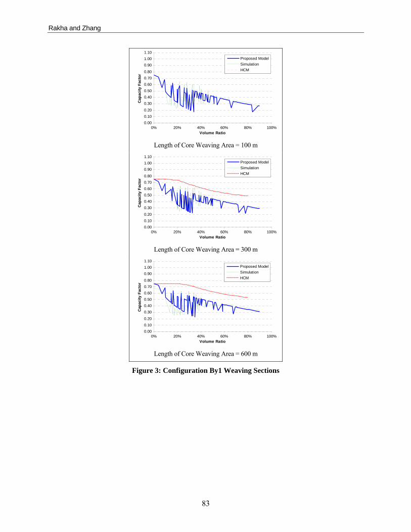
Rakha and Zhang

83

0% 20% 40% 60% 80% 100%0.000.100.20

0.300.400.500.600.700.80

0.901.001.10

Volume RatioC

apac

ity F

acto

r

Proposed ModelSimulationHCM

Length of Core Weaving Area = 100 m

0% 20% 40% 60% 80% 100%0.000.100.20

0.300.400.500.600.700.80

0.901.001.10

Volume Ratio

Cap

acity

Fac

tor

Proposed ModelSimulationHCM

Length of Core Weaving Area = 300 m

0% 20% 40% 60% 80% 100%0.000.100.20

0.300.400.500.600.700.80

0.901.001.10

Volume Ratio

Cap

acity

Fac

tor

Proposed ModelSimulationHCM

Length of Core Weaving Area = 600 m

Figure 3: Configuration By1 Weaving Sections

Rakha and Zhang

84

0% 20% 40% 60% 80% 100%0.000.100.20

0.300.400.500.600.700.80

0.901.001.10

Volume RatioC

apac

ity F

acto

r

Proposed ModelSimulationHCM

Length of Core Weaving Area = 100 m

0% 20% 40% 60% 80% 100%0.000.100.20

0.300.400.500.600.700.80

0.901.001.10

Volume Ratio

Cap

acity

Fac

tor

Proposed ModelSimulationHCM

Length of Core Weaving Area = 300 m

0% 20% 40% 60% 80% 100%0.000.100.20

0.300.400.500.600.700.80

0.901.001.10

Volume Ratio

Cap

acity

Fac

tor

Proposed ModelSimulationHCM

Length of Core Weaving Area = 600 m

Figure 4: Configuration Bz1 Weaving Sections

Rakha and Zhang

85

Relationship between Capacity Factor and VR (Site Bx2, weaving length of 100 m)

Relationship between t and Weaving Section Length

y = e-1.5033x

R2 = 0.7851

0.00

0.10

0.20

0.30

0.40

0.500.60

0.700.80

0.90

1.00

0% 20% 40% 60% 80% 100%

Volume Ratio (Weaving Volume/Total Volume)

Cap

acity

Fac

tor

y = 0.1525Ln(x) - 2.1141R2 = 0.9666

-1.6

-1.5

-1.4

-1.3

-1.2

-1.1

-1.0

-0.9

-0.80 100 200 300 400 500 600 700 800

Weaving Length (m)

t

Figure 5: Illustration of Model Development

Rakha and Zhang

86

Exponential Model HCM Procedures

Low Weaving Ratio Low Weaving Ratio

Medium Weaving Ratio Medium Weaving Ratio

High Weaving Ratio High Weaving Ratio

0

0.2

0.4

0.6

0.8

1

0 100 200 300 400 500 600 700 800

Weaving Section Length (m)

Cap

acity

Fac

tor

VR = 0.0 VR = 0.2VR = 0.4 VR = 0.6VR = 0.8 VR = 1.0

0

0.2

0.4

0.6

0.8

1

0 100 200 300 400 500 600 700 800

Weaving Section Length (m)

Cap

acity

Fac

tor

0

0.2

0.4

0.6

0.8

1

0 100 200 300 400 500 600 700 800

Weaving Section Length (m)

Cap

acity

Fac

tor

0

0.2

0.4

0.6

0.8

1

0 100 200 300 400 500 600 700 800

Weaving Section Length (m)

Cap

acity

Fac

tor

0

0.2

0.4

0.6

0.8

1

0 100 200 300 400 500 600 700 800

Weaving Section Length (m)

Cap

acity

Fac

tor

0

0.2

0.4

0.6

0.8

1

0 100 200 300 400 500 600 700 800Weaving Section Length (m)

Cap

acity

Fac

tor

Figure 6: Sensitivity Study Results from the Proposed Model and HCM Procedures for Configuration Bx2

87

Chapter 6. Estimating Weaving Section Capacity for Type B

Weaving Sections (It is being submitted to Transportation Research, Part B)

88

ESTIMATING WEAVING SECTION CAPACITY FOR TYPE B WEAVING SECTIONS

Yihua Zhang1 and Hesham Rakha2

ABSTRACT

The paper identifies 18 common configurations of Type B weaving sections and models them using the INTEGRATION software for a wide range of weaving lengths and travel demands. The developed models are compared with the 2000 Highway Capacity Manual procedures. The results demonstrate that the 2000 Highway Capacity Manual procedures suffer from a number of drawbacks. First, the procedures can only consider relatively long weaving sections (150 meters or longer). Second, the Highway Capacity Manual procedures fail to capture the impact of the distribution of weaving flows between freeway and on-ramp on the capacity of weaving sections. Third, capacity estimation from the Highway Capacity Manual procedures differs largely from simulation results, in both magnitude and patterns. By using the simulation results, four models are developed for improving the estimate of the capacity of Type B weaving sections, which include statistical and artificial neural network models. The paper demonstrates that the proposed models estimate the capacity to within 11% of the simulated data. Alternatively, the HCM procedures exhibit errors in the range of 114%.

Keywords: Freeway weaving sections, Capacity modeling, HCM 2000, Artificial Neural Networks, and INTEGRATION software.

INTRODUCTION

The freeway weaving analysis procedures in the 2000 Highway Capacity Manual (HCM) are based on research conducted in the early 1970s through the early 1980s (Roess and Ulerio, 2000). Subsequent research has shown that the method’s ability to predict the operation of a weaving section is limited (Lertworawanich and Elefteriadou, 2002, 2004), probably due to the outdated database. Other methods, such as gap-acceptance and simulation procedures, have been proposed as potential alternatives for estimating the capacity of weaving sections (Stewart et al., 1996; Kwon, Lau, and Aswegan, 2000; Lertworawanich and Elefteriadou, 2002, 2004).

The research effort that is presented in this paper utilized the INTEGRATION software, which has been demonstrated, to extent possible, to be valid for estimating the capacity of weaving sections by comparing to field data at a number of sites (Zhang and Rakha, 2005). This paper first identifies the sub-types and major configurations within Type B weaving sections according to the HCM 2000 procedures. The INTEGRATION software is then utilized to conduct a capacity analysis in which different weaving section lengths and traffic demands are considered for all configurations.

1 Charles Via Jr. Department of Civil and Environmental Engineering, Virginia Tech, E-mail: yihua@vt.edu. 2 Corresponding author. Charles Via Jr. Department of Civil and Environmental Engineering, Virginia Tech, 3500 Transportation Research Plaza (0536), Blacksburg, VA 24061. E-mail: hrakha@vt.edu.

Zhang and Rakha

89

Four capacity models are developed for each configuration and compared to the HCM procedures. Finally, a sensitivity analysis is performed in order to identify the impact of different parameters on the capacity of weaving sections.

INTEGRATION FRAMEWORK FOR MODELING WEAVING SECTIONS

The INTEGRATION software is a microscopic traffic simulation and assignment model that can represent traffic dynamics in an integrated freeway and traffic signal network. The model has been successfully applied since the early 1990s in North America and Europe. The INTEGRATION 2.30 lane-changing logic was described and validated against field data in an earlier publication (Rakha and Zhang, 2004). Furthermore, Zhang and Rakha (2005) demonstrated the validity of the INTEGRATION software for estimating the capacity of weaving sections by comparing simulation results to field-observed weaving section capacities. A brief description of these studies is presented in this section given that the INTEGRATION software serves as the basis of this study and thus it is important to demonstrate the credibility of this tool. It should be noted, however, that the authors recognize that no simulation tool can replicate reality perfectly; however it is impossible to gather in-field data on weaving sections for different configurations, with different demand distributions, and different weaving section lengths all operating at capacity. Consequently, a second best alternative is to utilize simulation to construct a database of data for the development of analytical models.

Rakha and Zhang (2004) utilized an empirical data set that was gathered in the late 1980s by the University of California at Berkeley (Cassidy et al., 1990). In this dataset, vehicle spatial distributions, both total and by movement, at successive reference points on nine weaving sites were gathered. The traffic movements included the four possible Origin-Destination (O-D) demands on freeway weaving sections, namely, Freeway-to-Freeway (FF), Freeway-to-Ramp (FR), Ramp-to-Freeway (RF), and Ramp-to-Ramp (RR) demands. The volume counts were provided at 5-minute intervals at a few reference points along the core weaving area. Using these data, the study demonstrated that lane-changing behavior within a weaving section is a very complicated phenomenon that is affected by many factors, including the geometric configuration of the weaving section, the O-D demand, and any upstream and downstream routing constraints. Rakha and Zhang demonstrated a high level of consistency between the INTEGRATION software and field data in the spatial and temporal distribution of lane-change intensity across the weaving lanes that was within the margin of daily variability (i.e., a margin of error of 250 veh/h). Consequently, the study concluded that the INTEGRATION software appeared to be appropriate for the modeling of weaving sections given that the temporal and spatial distribution of lane changes appeared to be consistent with field observations.

Zhang and Rakha (2005) validated the INTEGRATION software weaving section capacity estimates by comparing simulated capacity estimates to field-observed capacities. The study concluded that the capacity estimates of the INTEGRATION software were consistent with field data both in terms of magnitude and trend (mean average relative error less than 5%). Furthermore, the results demonstrated that the INTEGRATION capacity estimates were superior to the CORSIM and gap acceptance estimates when compared to field data. In addition, the study demonstrated that the weaving ratio, which is the ratio of the lowest weaving volume to the total weaving volume, has

Zhang and Rakha

90

a significant impact on the capacity of weaving sections. Unfortunately, the weaving ratio is not considered in the HCM 2000 capacity procedures. Furthermore, the study demonstrated that the length of weaving section has a larger impact on the capacity of weaving sections as the length of the weaving section decreases and the traffic demand increases. The study also demonstrated that there is no evidence to conclude that the speed differential between the freeway and ramp traffic has a significant impact on weaving section capacities. Finally, the study demonstrated that the HCM procedures for accounting for the impact of heavy duty vehicles on weaving section capacities are reasonable.

STATE-OF-THE-ART WEAVING ANALYSIS PROCEDURES

A limited number of publications were found in the literature that were deemed related to this study. For example, Zarean and Nemeth (1988) utilized the WEAVSIM microscopic simulation model to investigate the effect of the different arrival speeds on the operation of weaving sections. Subsequently, the researchers developed a regression model for the modeling of weaving sections based on the simulation results. The simulation results demonstrated that the speed differential between the mainline and on-ramp arrivals had a significant effect on the operation of weaving sections, which was not considered in the 1985 HCM procedures (Transportation Research Board, 1985) and is not considered in the current HCM procedures (Transportation Research Board, 2000). However, these findings are not consistent with the findings of Zhang and Rakha (2005) that was described earlier.

Skabardonis et al. (1989) modified the INTRAS microscopic simulation model to predict the speeds of weaving and non-weaving vehicles for eight major freeway weaving sections. Vehicle speeds within the weaving sections were compared to a few analytical procedures, including the 1985 HCM procedure, Leisch’s procedure, JHK’s procedure, Fazio’s Procedure, and the Polytechnic Institute of New York (PINY) procedure. The researchers concluded that the INTRAS speed predictions were closer to the field measurements than the analytical procedure speed predictions. Thus the researchers concluded that simulation tools could be utilized with field data to enhance existing state-of-the-art analytical procedures for the modeling of weaving section operations.

Stewart, Baker, and Van Aerde (1996) evaluated the capability of INTEGRATION version 1.50 for the modeling of weaving sections. The study showed that both the 1985 HCM procedure and INTEGRATION offered identical conclusions for a given sample problem. However, the study demonstrated differences between the two approaches on critical design parameters of weaving sections. Specifically, INTEGRATION identified the number of lanes in the core area as a critical factor that affects the capacity of weaving sections, which is currently not captured in the HCM procedures. Alternatively, while the HCM procedures demonstrated that the length of the core area was critical in the design of weaving sections, the INTEGRATION results demonstrated that this factor was critical for short lengths but was less critical as the weaving section length increased.

Vermijs (1998) reported on the efforts in developing the Dutch capacity standards for freeway weaving sections using FOSIM (Freeway Operations SIMulation), a microscopic simulation software developed in the Netherlands. Specifically, a total of 315 Type A weaving sections with different configurations and traffic factors were simulated. All simulation runs were repeated 100

Zhang and Rakha

91

times using different random seeds. The 100 simulation results for capacity appeared to be normally distributed with standard deviation in the range of about 200–400 veh/h/lane.

Finally, Lertworawanich and Elefteriadou (2002, 2003) proposed a capacity estimation method for weaving sections based on gap acceptance and linear optimization techniques. Readers interested in the specific details of the procedure are encouraged to review the literature. It should be noted, however that the gap acceptance method makes a number of simplifying assumptions that limit the applicability of the procedures. For example, the procedures do not capture the effect of the weaving section length on the capacity of weaving sections.

IDENTIFIED CONFIGURATIONS AND SIMULATION SETTING

According to the HCM 2000, it is the lane changing required of weaving vehicles that characterizes Type B weaving sections. Specifically, if one weaving movement can be made without making any lane changes and the other weaving movement requires at most a single lane change, such a section is characterized as a Type B weaving section.

In this study, three sub-types within Type B weaving sections, termed Bx, By, and Bz, were identified according to the minimum number of lane changes required by the two weaving movements. Sub-type Bx weaving sections require only one lane change for one of the freeway to off-ramp and on-ramp to freeway movements and no lane changes for the other weaving movement, while Sub-type By has a shared lane at the entry gore, with no lane balance at the exit gore. Sub-type Bz has a shared lane at the entry gore and lane balance at the exit gore. Because Type B weaving sections usually have three, four, or five lanes in the core area, 18 configurations were investigated in this study, as shown in Figure 1.

In terms of the simulation runs, the input free-flow speed along the freeway was set at 110 km/h, while the free-flow speed on the ramps was set at 90 km/h if the ramp was a single lane; otherwise the ramp free-flow speed was set at 110 km/h. These speeds appear to be common speeds on North American freeways. No heavy vehicles were considered as part of the analysis because Zhang and Rakha (2005) demonstrated that the heavy vehicle factor within the HCM 2000 procedures efficiently captures the effects of heavy vehicles on the capacity of weaving sections and thus these can be utilized to adjust the weaving section capacity. The lane capacity was set at 2,350 and 2,000 veh/h/lane for facilities with free-flow speeds of 110 km/h and 90 km/h, respectively, which is consistent with the HCM 2000 procedures. The speed-at-capacity was set at 80% of the free speed, which has been demonstrated to be the norm on North American freeways (Rakha and Van Aerde, 1995; Rakha and Crowther, 2003).

EXPERIMENTAL DESIGN

As was mentioned earlier, the study utilized the INTEGRATION software to conduct the analysis. The capacity of the weaving section was estimated by increasing the traffic demand uniformly and recording the maximum 15-minute volume that was able to proceed through the weaving section.

Zhang and Rakha

92

The first step in this study was to simulate all 18 configurations in INTEGRATION with different weaving section lengths and different Origin-Destination (O-D) demands. Weaving section lengths of 50, 75, 100, 150, 300, 450, 600, and 750 meters were considered, which covered the maximum range of HCM 2000 procedures in addition to lengths shorter than what is considered in the HCM procedures.

There are four possible traffic movements at a freeway weaving section: freeway-to-freeway (FF), freeway to off-ramp (FR), on-ramp to freeway (RF), and on-ramp to off-ramp (RR) movements. It is obvious that a change in the O-D pattern (different traffic mix of FF:FR:RF:RR) may result in a change in the weaving section capacity because of differences in the level of turbulence within the weaving section. An attempt was made to cover the entire possible range of O-D demands including the extreme conditions when the weaving section converges to a merge or diverge section. The coverage of these extreme conditions ensures that the modeling of weaving section capacity is consistent with the modeling of merge and diverge sections because these scenarios represent a special case of the weaving section O-D demand. Specifically, a merge scenario only includes FF and RF demands while a diverge scenario only includes FF and FR demands.

In this study uncertainty of traffic demands and the impact of this uncertainty is not considered, though some of the techniques like neural network can deal with this uncertainty.

SIMULATION RESULTS

As stated before, for each configuration, a wide variety of traffic conditions and core weaving area lengths were simulated using the INTEGRATION software. The simulated capacities were computed based on the maximum 15-minute flow rate that proceeds through the weaving section by systematically increasing the O-D demand. Alternatively, the HCM capacities were calculated according to the capacity tables (Exhibit 24-8) in Chapter 24 of the HCM 2000 using interpolation. Because the HCM 2000 procedures do not cover weaving section lengths of 50, 75, and 100 meters and only consider a maximum volume ratio of 80%, the simulation scenarios went beyond the confines of the HCM procedures.

In order to generalize the results of this study to consider differing basic freeway section and ramp capacities, a capacity factor was computed. The capacity factor was computed as the weaving section capacity divided by the capacity directly upstream of the weaving section (sum of upstream freeway and on-ramp capacities). As an example, the incoming capacity for configuration Bx2 is 3 × 2,350 + 2 × 2,350 = 11,750 veh/h. Consequently, a factor of 1.0 reflects a weaving section capacity that is equal to the capacity upstream of the weaving section.

For ease of comparison between simulated and HCM capacity estimates, the capacities derived from the HCM procedures were also normalized by the incoming capacity. Due to space limitation, only the results for configuration Bx2 are shown in Figure 2, and only weaving lengths of 150, 450, and 750 meters are illustrated. The results from other configurations show similar patterns as configuration Bx2. The figure clearly demonstrates that the differences between the simulated and HCM capacity estimates are significant. For example, the HCM procedures demonstrate that the volume ratio has no impact on the weaving section capacity for small volume ratios. This trend, however, was not observed in the simulation results. Furthermore, the simulated capacity estimates

Zhang and Rakha

93

demonstrate a zigzag pattern that may appear as noise in the data at first glance. However, these zigzags reflect other factors that affect the weaving section capacity, including the weaving ratio. For example, Zhang and Rakha (2005) demonstrated that the weaving ratio does have a significant impact on the capacity of freeway weaving sections.

Figure 2 also clearly demonstrates that the HCM capacity estimates are higher than the simulated capacity estimates. Given that the INTEGRATION weaving section estimates have been demonstrated to be consistent with field data (error of approximately 5%) (Zhang and Rakha, 2005) it is fair to conclude that the HCM procedures tend to overestimate the capacity of weaving sections.

MODEL DEVELOPMENT

Based on the above analysis, it is evident that new procedures are required to estimate the capacity of weaving sections. Four capacity models are developed as part of this research effort, namely: two statistical models and two ANN models. Each of these models will be described in detail later in the paper.

The HCM 2000 defines the weaving ratio as the ratio of the smaller of the two weaving flows to the total weaving flow. This definition does not distinguish between the FR and RF weaving flows. For example, there are two possible situations for a weaving ratio of 0.30. One possibility is that the FR demand constitutes 30% of the total weaving volume; the other is that the RF demand constitutes 30% of the total weaving flow. An analysis of the simulation results revealed significant differences in weaving section capacity estimates depending on the source of the weaving volume (FR or RF). In other words, the weaving ratio distribution is asymmetric. In this model, we introduced a new definition of the weaving ratio as

( )FWR FR FR RF= + [1]

Model 1: Exponential Model

The first version of this model was introduced in an earlier paper (Rakha and Zhang, 2005). It has an exponential function format shown in Equation 2; where F is the capacity factor, x is the length of the weaving section in meters, VR is the volume ratio, and a, b, and c are calibrated model coefficients.

( ln )b x c VRF a e += ⋅ [2]

In the first version of this model, two threshold values were used to define three regimes corresponding to merging, weaving, and diverging conditions. The current research, however, proposes an enhanced version of this model. Rather than using threshold values to construct a piece-wise model, the impact of the weaving ratio is modeled by continuous sine functions. The simulation results of site Bx2 considering a 750-m core area is used to illustrate the development of this model. As shown in Figure 3, the trend line of the simulation results can be modeled using an exponential decay function. The difference between the exponential function and simulation results

Zhang and Rakha

94

is also shown as a dotted line in Figure 3. This difference resembles a sine function, thus it was modeled as the product of two sine functions, one representing the magnitude of the difference and the other capturing the difference frequency. Thus, the model has the form shown in Equation 3. The proposed capacity model parameters are summarized in Table 1.

( ) ( )2 3( ln )1 4 5 6sin sina x a VRF a e a WR a aVR+= ⋅ + ⋅ + [3]

The 95% confidence intervals of all the model coefficients were computed and summarized in Table 2. The insignificant parameters (parameters with intervals that include 0) are highlighted in the table. The results demonstrate that apart from a single parameter in one of the models all parameters are significant. Consequently, this parameter is maintained in order to ensure model structure consistency for the different network configurations.

Model 2: Angle Model

During the development of the angle model, the contour plot of the capacity factor as a function of the WR and VR factors for each of the studied lengths was investigated. These contour plots of lengths of 50, 150, 450, and 750 meters for configuration Bx2 are shown in Figure 4. It is obvious that the extension lines of almost all the contour lines pass through or by a single point, which is denoted as P0 in Figure 5. This implies that there is a strong relationship between the capacity factor and the angle θ, which is also shown in Figure 5. The coordinates of point P0 can be obtained by assuming a relationship between angle θ and the capacity factor, using least squared optimization approach.

To account for the impact of weaving section length on capacity factor, the relationship of capacity factor and weaving section length was inherited from the exponential model. Because the exponential of a first order polynomial of lnx is equivalent to a power function of x, volume ratio was taken into account as a power function. Figure 6 illustrates the relationship between capacity factor and angle θ. A second order polynomial function can model this relationship very well. This determined that the capacity can be modeled as Equation 4. The coefficients a1, a2, a3, a4, a5, b1, and b2 can be obtained by minimizing sum of squared error between the capacity estimates and the simulation results. The estimated coefficients of this model are summarized in Table 3.

( ) 521 2 3 4( )aF a a a x aθ θ= + + + [4]

Where 1 1

2 21 2

cos( ) ( )

VR b

VR b b WRθ −

⎛ ⎞⎟−⎜ ⎟⎜= ⎟⎜ ⎟⎜ ⎟⎟⎜ − + −⎝ ⎠

The 95% confidence intervals of all the model coefficients were found to be significant, as demonstrated in Table 4.

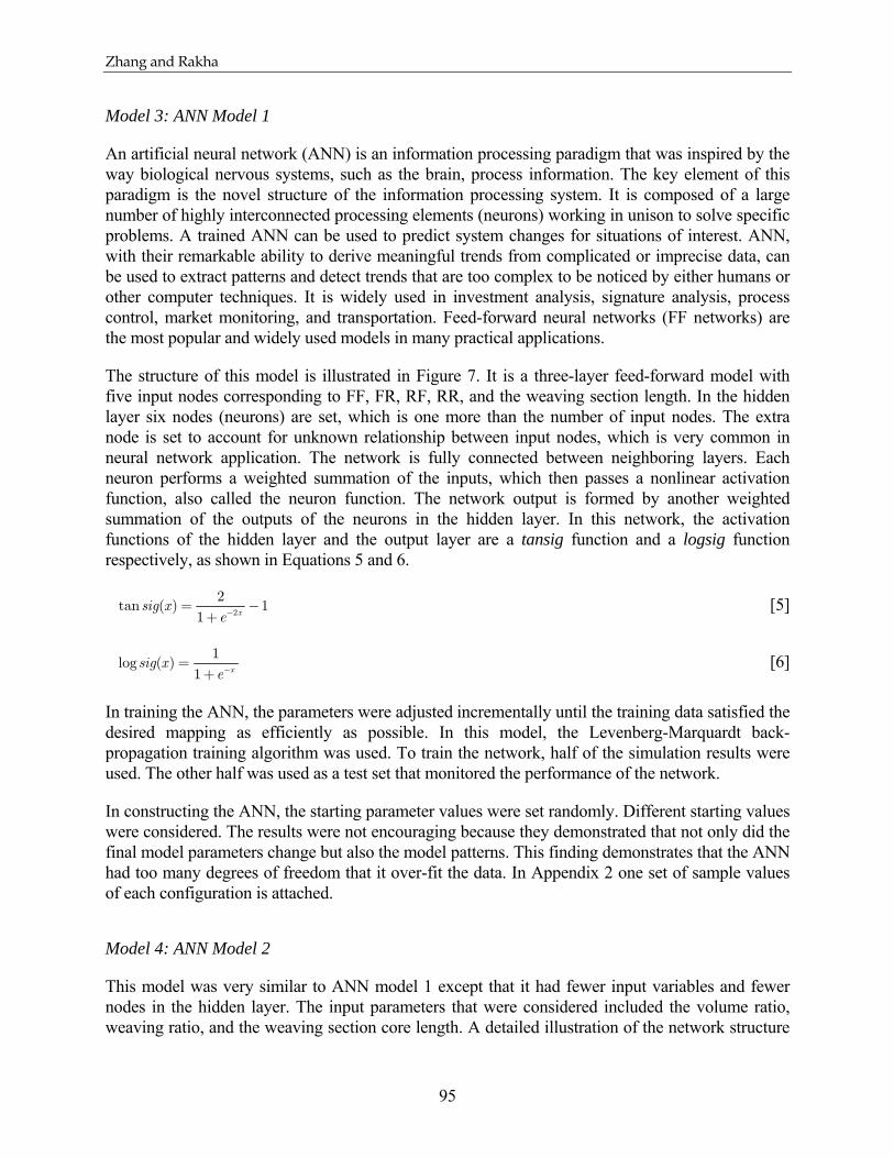
Zhang and Rakha

95

Model 3: ANN Model 1

An artificial neural network (ANN) is an information processing paradigm that was inspired by the way biological nervous systems, such as the brain, process information. The key element of this paradigm is the novel structure of the information processing system. It is composed of a large number of highly interconnected processing elements (neurons) working in unison to solve specific problems. A trained ANN can be used to predict system changes for situations of interest. ANN, with their remarkable ability to derive meaningful trends from complicated or imprecise data, can be used to extract patterns and detect trends that are too complex to be noticed by either humans or other computer techniques. It is widely used in investment analysis, signature analysis, process control, market monitoring, and transportation. Feed-forward neural networks (FF networks) are the most popular and widely used models in many practical applications.

The structure of this model is illustrated in Figure 7. It is a three-layer feed-forward model with five input nodes corresponding to FF, FR, RF, RR, and the weaving section length. In the hidden layer six nodes (neurons) are set, which is one more than the number of input nodes. The extra node is set to account for unknown relationship between input nodes, which is very common in neural network application. The network is fully connected between neighboring layers. Each neuron performs a weighted summation of the inputs, which then passes a nonlinear activation function, also called the neuron function. The network output is formed by another weighted summation of the outputs of the neurons in the hidden layer. In this network, the activation functions of the hidden layer and the output layer are a tansig function and a logsig function respectively, as shown in Equations 5 and 6.

2

2tan ( ) 1

1 xsig x

e−= −

+ [5]

1log ( )

1 xsig x

e−=

+ [6]

In training the ANN, the parameters were adjusted incrementally until the training data satisfied the desired mapping as efficiently as possible. In this model, the Levenberg-Marquardt back-propagation training algorithm was used. To train the network, half of the simulation results were used. The other half was used as a test set that monitored the performance of the network.

In constructing the ANN, the starting parameter values were set randomly. Different starting values were considered. The results were not encouraging because they demonstrated that not only did the final model parameters change but also the model patterns. This finding demonstrates that the ANN had too many degrees of freedom that it over-fit the data. In Appendix 2 one set of sample values of each configuration is attached.

Model 4: ANN Model 2

This model was very similar to ANN model 1 except that it had fewer input variables and fewer nodes in the hidden layer. The input parameters that were considered included the volume ratio, weaving ratio, and the weaving section core length. A detailed illustration of the network structure

Zhang and Rakha

96

is illustrated in Figure 8. And a set of sample values of each configuration is attached in Appendix 3.

MODEL VALIDATION

Following the development of the analytical models, the next step is to investigate the model performance for different random number seeds, estimate the prediction error, and validate the model results against independent field observations.

Analysis of Capacity Variability

To test the impact of random seeds on the simulation results, configuration Bx2 was simulated using 10 different random seeds (0, 100, 200, 300, 400, 500, 600, 700, 800, and 900). In quantifying the impact of the random number seed on the model performance, four error measures were estimated. These error measures were the mean relative error (MeRE), the maximum relative error (MaRE), the mean absolute error (MeAE), and the maximum absolute error (MaAE). The errors were derived as

( )1

n

s m Si

MeRE y y y n=

= −∑ [7]

( )max s m SMaRE y y y= − [8]

( )1

n

s mi

MeAE y y n=

= −∑ [9]

( )max s mMaAE y y= − [10]

where ys is the capacity factor based on the simulation results, ym is capacity factor based on the proposed model, and n is the number of observations.

The performance of the proposed models for configuration Bx2 is summarized in Table 5. It is shown in the table that the model efficiency is not impacted by the random number seed. Consequently, the issue of randomness is not pursued any further in this research effort.

Validation of Proposed Models

After developing the models, the next step in the analysis was to validate the models. Table 6 summarizes the differences between the proposed model capacity factor estimates against the simulation results for all 18 type B configurations. The corresponding results from the HCM procedures are also shown in Table 6 for comparison purposes. Alternatively, Table 7 provides some summary statistics for the results of Table 6. Table 7 demonstrates that the ANN models provide an excellent match with the simulation results for all 18 configurations (MeAE of 0.01 and 0.02, respectively) while the statistical models offered a slightly lower fit (MeAE of 0.03). The

Zhang and Rakha

97

average MeRE was 6, 6, 3, and 5 percent for models 1 through 4, respectively, which represents a considerable improvement over the HCM model estimates (average MeRE of 57 percent). Thus the proposed models offer significant improvements to the current state-of-the-art procedures.

Figure 9 presents the capacity factor from proposed models, HCM procedures, and simulation results for configuration Bx2 considering a weaving section length of 300 meters. It is clear that all the proposed models are superior to the HCM procedures. However, it should be emphasized that these comparisons are made against the simulation results that were utilized to develop the models. Consequently, the next validation effort involves direct comparisons against field data.

The models were also tested on a Type B weaving section on the Queen Elizabeth Expressway (QEW) in Toronto, Canada (Lertworawanich and Elefteriadou, 2004). It has the geometry of configuration Bx4 with a length of 550 meters. The posted speed limit on the QEW was 100 km/h at the time of the study with a 10 percent heavy vehicle population. The selected site operated under congested conditions because of the intense lane changing behavior within the weaving section. The section capacity and total traffic demand classified by on-ramp, off-ramp, upstream mainline, and downstream mainline flows were recorded in a data set. The weaving section capacity was computed as the maximum observed pre-breakdown 15-minute flow rate. The data set included 10 days of data. From the percentage of traffic on all the four legs of the weaving section, a range of possible O-D demands can be deducted. By evaluating the O-D demands with all the models, a band of possible capacity factors can be obtained for each capacity model. The results are shown in Figure 10. It shows that for exponential model, angle model, ANN model 1, and ANN model 2, most of the field capacity data are covered by the band of each model. But for HCM procedures, none of the field capacity data is covered by the band. HCM procedures tend to over-estimate the capacity of Type B weaving sections, which is consistent with the conclusion drawn by Lertworawanich and Elefteriadou. We can conclude that the proposed models perform better than HCM procedures.

SENSITIVITY ANALYSIS RESULTS

A sensitivity analysis was conducted using the proposed models together with the HCM procedures in an attempt to characterize the behavior of these models as the independent variables vary. These independent factors included the weaving section length, volume ratio, and weaving ratio. Here, configuration Bx2 is again used to illustrate the results.

First, the relationship between the weaving section length and the capacity factor was studied by maintaining a constant weaving ratio of 0.50 while varying the weaving section length from 50 to 750 meters and the volume ratio from 0.0 to 1.0. The results from HCM procedures and the four proposed models are shown in Figure 11. For all the proposed models and HCM procedures, generally the capacity factor increases as the weaving section length increases. It is worth mentioning that when the volume ratio is zero, that regardless of the weaving section length, the capacity factor should remain at 1.0. Based on this fact only the HCM and the exponential model perform well.

Another point is that as the weaving section length increases, the capacity factor tends to be constant for exponential model and angle model, which implies that the influence of weaving

Zhang and Rakha

98

section length is reduced as the length of the weaving section increases. This conclusion appears to be very reasonable and intuitive. Alternatively, the two ANN models together with the HCM procedures produce a less evident trend. As for the magnitude of capacity factor, it is obvious from these figures that both the HCM procedures and ANN model 1 produce higher capacity factors in comparison to the other three models.

The next step in the analysis was to characterize the relationship between the volume ratio and the capacity factor. To study this relationship, the weaving section length was kept constant at 300 meters, while the volume ratio and weaving ratio were each varied from 0.0 to 1.0. The HCM procedure results and the four proposed models are shown in Figure 12. Because the HCM procedures ignore the impact of the weaving ratio on the capacity of weaving sections, there is only a single curve displayed in Figure 12. The results demonstrate that this simplification has significant impacts on the efficiency of the HCM procedures. Results from the HCM procedures show that weaving sections can tolerate volume ratios up to 0.1 without any decrease in capacity, while the other four models show that the weaving section experiences almost the sharpest decrease between volume ratios of 0.0 to 0.2. When volume ratio is 0, the capacity factor should be identical for different weaving ratios; on this point angle model and ANN model 2 do not perform as well as the other two proposed models. Furthermore, the curves produced by ANN model 1 exhibit unrealistic behaviors.

The distribution of simulated data points for each configuration is plotted in the VR-WR plane, as illustrated in Figure 13. For each configuration, 100 points are shown. Though the intent of this study was to cover the entire VR-WR space, this was not possible because of capacity restrictions on the entry and exit roadways. The theoretical distribution of possible traffic conditions is restricted by two curves for each configuration when the incoming legs of a weaving section are loaded to the same volume-to-capacity ratio. In other words, when upstream freeway and on-ramp are loaded with traffic proportional to their capacity, it is impossible for the point of volume rate and weaving ratio to locate to the right of the two curves in Figure 13. From Figure 13 we can see that the traffic conditions considered in this study are distributed in most of the feasible area left to the two curves for each configuration.

Figure 14 demonstrates the distribution of both the demand points and throughput points for configuration Bx2 considering a weaving section length of 450 meters. In this figure the corresponding demand and throughput are connected with a line. The length of the line may be viewed as an indicator of the difference between the corresponding demand and actual throughput condition. The figure demonstrates that some lines are of significant lengths, which means that in the corresponding simulation scenarios some O-D demands are restricted more than other O-D demands by the weaving section configuration. Figure 15 shows the distribution of the (VR, WR) points of throughput for all configurations. In this figure we observe a significant difference from those in Figure 13.

In order to capture the reduced feasible space, the sensitivity analysis that was presented earlier in Figure 12 is reconstructed and displayed in Figure 16. The results of Figure 16 are consistent with those of Figure 12.

Zhang and Rakha

99

CALIBRATION OF MODELS BASED ON THROUGHPUT

Based on the above analysis we found that the composition of throughput volume at core weaving area is different from that of demands. To make the proposed capacity models more useful, they are also calibrated with throughput. The coefficients of exponential model and angle model are shown in Table 8 and Table 9 respectively. For the same reason stated before, the coefficients for ANN models based on throughput are not shown in this paper. Table 10 shows the modeling errors for all the four models that were calibrated with throughput and Table 11 shows the statistics of Table 10, which includes maximum, minimum, and average values. It is obvious that the models calibrated with throughput perform as well as those calibrated with demands.

FINDINGS AND CONCLUSIONS

The research presented in this paper examined one of the most important aspects of analysis of freeway weaving sections, namely the capacity analysis. The researchers investigated the capacity of Type B weaving sections using simulation. The simulation results demonstrate that the HCM procedures are not only inadequate but fail to capture critical variables that impact the capacity of weaving sections, including the weaving ratio and the distribution of the weaving volume between freeway-to-ramp and ramp-to-freeway. The HCM procedures tend to over estimate the capacity of Type B weaving sections from both the study presented in this paper and the paper of Lertworawanich and Elefteriadou (2004).

The researchers developed four models for estimating the capacity of Type B weaving sections. In these models, a new definition of the weaving ratio was introduced (FR/(FR+RF)) that explicitly accounts for the source of the weaving volume.

The proposed analytical models estimate the capacity of weaving sections to within 11% of the simulated data. Alternatively, the HCM procedures exhibit errors in the range of 114%. Among the four newly developed models, ANN models performed slightly better than the statistical models in terms of model prediction errors. However, the sensitivity analysis results demonstrated unrealistic behavior of the ANN models under certain conditions. Consequently, we propose the use of model 1 since it provides a high level of accuracy with realistic behavior as a function of changes in the model input parameters.

ACKNOWLEDGEMENTS

The authors acknowledge the financial support of the Mid-Atlantic University Transportation Center (MAUTC) and the Virginia Department of Transportation in conducting this research effort.

REFERENCES

Bacon, V., Lovell, D., May, A., and Van Aerde, M.. (1994) Use of INTEGRATION model to study high-occupancy-vehicle facilities. Transportation Research Record, No. 1446, 8-13.

Zhang and Rakha

100

Cassidy, M., Chan, P., Robinson, B., and A. D. May (1990), A Proposed Analytical Technique for the Design and Analysis of Major Freeway Weaving Sections, Institute of Transportation Studies, University of California-Berkeley, research Report UCB-ITS-RR-90-16.

Dion F., Rakha H., and Zhang Y. (2004), Evaluation of potential transit signal priority benefits along a fixed-time signalized arterial. ASCE Journal of Transportation Engineering, Vol 130, pp. 294-303.

Gardes, Y. and May, A. D. (1993) Simulation of IVHS on the Smart Corridor Using the INTEGRATION Model: Initial Investigation. PATH Research Report, UCB-ITS-PRR-93-3.

Hellinga, B. and Van Aerde, M. (1994) An overview of a simulation study of the Highway 401 freeway traffic management system. Canadian Journal of Civil Engineering, 21. 439-454.

Kwon, E., Lau, R., and Aswegan, J. (2000) Maximum possible weaving volume for effective operations of ramp-weave areas, Transportation Research Record, n 1727, 132-141.

Lertworawanich, P. and Elefteriadou, L. (2002) Capacity estimations for Type-B weaving areas based on gap acceptance. Transportation Research Record, 1776, 24-34.

Lertworawanich, P. and Elefteriadou, L. (2003) Methodology for estimating capacity at ramp weaves based on gap acceptance and linear optimization. Transportation Research Part B: Methodological, 37, 459-483.

Lertworawanich, P. and Elefteriadou, L. (2004) Evaluation of three freeway weaving capacity estimation methods and comparison to field data, freeway capacity. Compendium of papers (CD-ROM) presented at the 83rd annual meeting of the Transportation Research Board, Washington, D.C.

Rakha H. and Crowther B. (2003), Comparison and Calibration of FRESIM and INTEGRATION Steady-state Car-following Behavior, Transportation Research, 37A, pp. 1-27.

Rakha, H. and Ahn, K. (2004) The INTEGRATION modeling framework for estimating mobile source emissions. ASCE Journal of Transportation Engineering, 130(2), 183-193.

Rakha, H., Medina, A., Sin, H., Dion, F., Van Aerde, M., and Jenq, J. (2000) Coordination of traffic signals across jurisdictional boundaries: Field and simulation results. Paper presented at the 79th annual meeting of the Transportation Research Board, Washington D.C., CD-ROM, paper # 00-1560.

Rakha, H., Van Aerde, M., Bloomberg, L., and Huang, X. (1998) Construction and calibration of a large-scale micro-simulation model of the Salt Lake area. Paper presented at the 77th annual meeting of the Transportation Research Board, Washington, D.C.

Rakha H. and Van Aerde M., Statistical Analysis of Day-to-Day Variations in Real-Time Traffic Flow Data, Transportation Research Record, No. 1510, pp. 26-34, 1995.

Rakha, H. and Zhang, Y. (2004) The INTEGRATION 2.30 framework for modeling lane-changing behavior in weaving sections, Paper presented at the 83rd annual meeting of the Transportation Research Board, Washington, D.C., paper # 04-3422.

Rakha, H. and Zhang, Y. (2005) Capacity modeling for Type B weaving sections. Paper presented at the 84th annual meeting of the Transportation Research Board, paper # 05-2483.

Zhang and Rakha

101

Roess, R. and Ulerio, J. (2000) Weaving area analysis in year 2000 Highway Capacity Manual. Transportation Research Record, n 1710, 145-153.

Skabardonis, A., Cassidy, M., May, A. D., and Cohen, S. (1989) Application of simulation to evaluate the operation of major freeway weaving sections. Transportation Research Record, 1225, 91-98.

Stewart, J., Baker, M., and Van Aerde, M. (1996) Evaluating weaving section designs using INTEGRATION, Transportation Research Record, 1555, 33-41.

Transportation Research Board, National Research Council. (1985) Special Report 209: Highway Capacity Manual. Washington, D.C.

Transportation Research Board, National Research Council. (2000) Highway Capacity Manual (HCM) 2000 – Weaving Segments, Chapter 24. Washington, D.C.

Vermijs, R. (1988) New Dutch capacity standards for freeway weaving sections based on micro simulation. Proceedings of the Third International Symposium on Highway Capacity, pp. 1065-1080.

Zarean, M. and Nemeth, Z. A. (1988) WEASIM: A microscopic simulation model of freeway weaving sections. Transportation Research Record, n 1194, 48-54.

Zhang, Y. and Rakha, H. (2005) Systematic analysis of capacity of weaving sections. Paper presented at the 84th annual meeting of the Transportation Research Board, paper # 05-0916.

Zhang and Rakha

102

Table 1: Exponential Model for Type B Weaving Sections Configuration Exponential Model

Bx1 ( ) ( )VRWReF VRx 53.2sin47.328.0sin98.0 )91.2ln21.0( −+= −

Bx2 ( ) ( )VRWReF VRx 53.2sin57.334.0sin01.1 )05.4ln31.0( −+= −

Bx3 ( ) ( )VRWReF VRx 69.2sin29.314.0sin97.0 )63.2ln19.0( −+= −

Bx4 ( ) ( )(0.12ln 1.76)0.97 sin 0.11 3.08 sin 3.89x VRF e WR VR−= − +

Bx5 ( ) ( )(0.09ln 1.32)0.96 sin 0.23 3.25 sin 3.80x VRF e WR VR−= + −

Bx6 ( ) ( )(0.09ln 1.33)0.96 sin 0.23 3.02 sin 3.77x VRF e WR VR−= − +

Bx7 ( ) ( )(0.20ln 2.67)0.98 sin 0.04 3.19 sin 2.61x VRF e WR VR−= − +

Bx8 ( ) ( )(0.11ln 1.88)0.96 sin 0.15 3.07 sin 4.36x VRF e WR VR−= − +

By1 ( ) ( )VRWReF VRx 24.2sin54.334.0sin73.0 )87.3ln24.0( −+= −

By2 ( ) ( )VRWReF VRx 37.4sin29.336.0sin73.0 )04.2ln14.0( −+= −

By3 ( ) ( )VRWReF VRx 50.7sin20.318.0sin76.0 )77.1ln10.0( −+= −

By4 ( ) ( )VRWReF VRx 40.2sin70.351.0sin83.0 )17.6ln42.0( −+= −

By5 ( ) ( )VRWReF VRx 77.2sin27.309.0sin77.0 )45.3ln21.0( +−= −

By6 ( ) ( )VRWReF VRx 12.6sin23.322.0sin77.0 )91.1ln09.0( −+= −

Bz1 ( ) ( )VRWReF VRx 16.2sin21.302.0sin73.0 )82.1ln09.0( −+= −

Bz2 ( ) ( )VRWReF VRx 59.2sin24.313.0sin77.0 )09.3ln18.0( +−= −

Bz3 ( ) ( )VRWReF VRx 15.4sin08.319.0sin77.0 )28.2ln16.0( +−= −

Bz4 ( ) ( )VRWReF VRx 19.8sin16.307.0sin76.0 )01.2ln11.0( −+= −

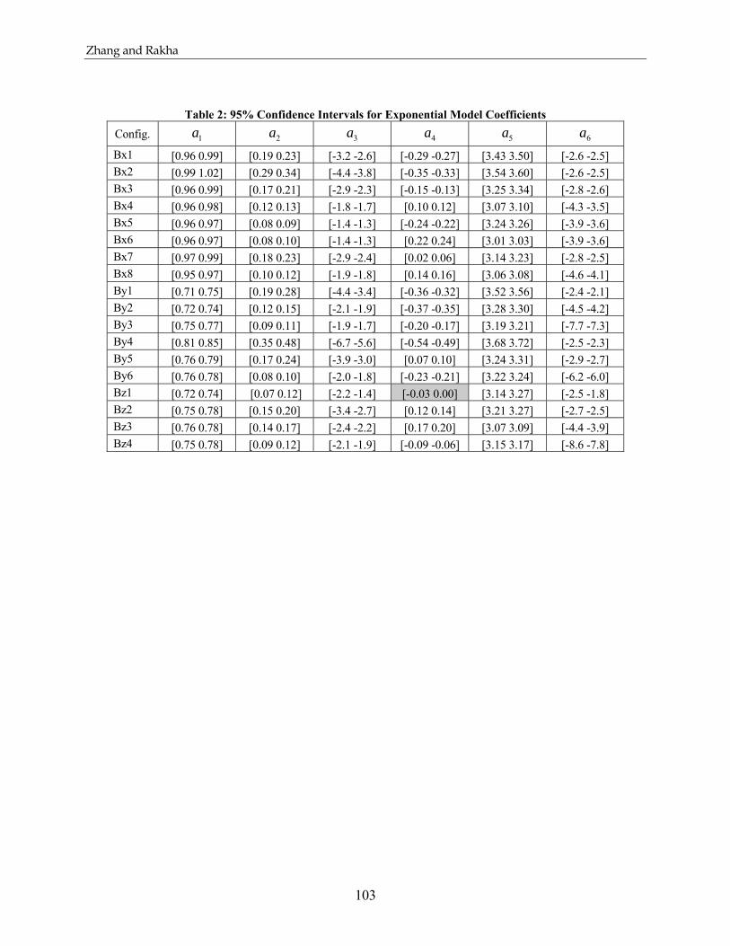
Zhang and Rakha

103

Table 2: 95% Confidence Intervals for Exponential Model Coefficients Config. 1a 2a 3a 4a 5a 6a

Bx1 [0.96 0.99] [0.19 0.23] [-3.2 -2.6] [-0.29 -0.27] [3.43 3.50] [-2.6 -2.5] Bx2 [0.99 1.02] [0.29 0.34] [-4.4 -3.8] [-0.35 -0.33] [3.54 3.60] [-2.6 -2.5] Bx3 [0.96 0.99] [0.17 0.21] [-2.9 -2.3] [-0.15 -0.13] [3.25 3.34] [-2.8 -2.6] Bx4 [0.96 0.98] [0.12 0.13] [-1.8 -1.7] [0.10 0.12] [3.07 3.10] [-4.3 -3.5] Bx5 [0.96 0.97] [0.08 0.09] [-1.4 -1.3] [-0.24 -0.22] [3.24 3.26] [-3.9 -3.6] Bx6 [0.96 0.97] [0.08 0.10] [-1.4 -1.3] [0.22 0.24] [3.01 3.03] [-3.9 -3.6] Bx7 [0.97 0.99] [0.18 0.23] [-2.9 -2.4] [0.02 0.06] [3.14 3.23] [-2.8 -2.5] Bx8 [0.95 0.97] [0.10 0.12] [-1.9 -1.8] [0.14 0.16] [3.06 3.08] [-4.6 -4.1] By1 [0.71 0.75] [0.19 0.28] [-4.4 -3.4] [-0.36 -0.32] [3.52 3.56] [-2.4 -2.1] By2 [0.72 0.74] [0.12 0.15] [-2.1 -1.9] [-0.37 -0.35] [3.28 3.30] [-4.5 -4.2] By3 [0.75 0.77] [0.09 0.11] [-1.9 -1.7] [-0.20 -0.17] [3.19 3.21] [-7.7 -7.3] By4 [0.81 0.85] [0.35 0.48] [-6.7 -5.6] [-0.54 -0.49] [3.68 3.72] [-2.5 -2.3] By5 [0.76 0.79] [0.17 0.24] [-3.9 -3.0] [0.07 0.10] [3.24 3.31] [-2.9 -2.7] By6 [0.76 0.78] [0.08 0.10] [-2.0 -1.8] [-0.23 -0.21] [3.22 3.24] [-6.2 -6.0] Bz1 [0.72 0.74] [0.07 0.12] [-2.2 -1.4] [-0.03 0.00] [3.14 3.27] [-2.5 -1.8] Bz2 [0.75 0.78] [0.15 0.20] [-3.4 -2.7] [0.12 0.14] [3.21 3.27] [-2.7 -2.5] Bz3 [0.76 0.78] [0.14 0.17] [-2.4 -2.2] [0.17 0.20] [3.07 3.09] [-4.4 -3.9] Bz4 [0.75 0.78] [0.09 0.12] [-2.1 -1.9] [-0.09 -0.06] [3.15 3.17] [-8.6 -7.8]

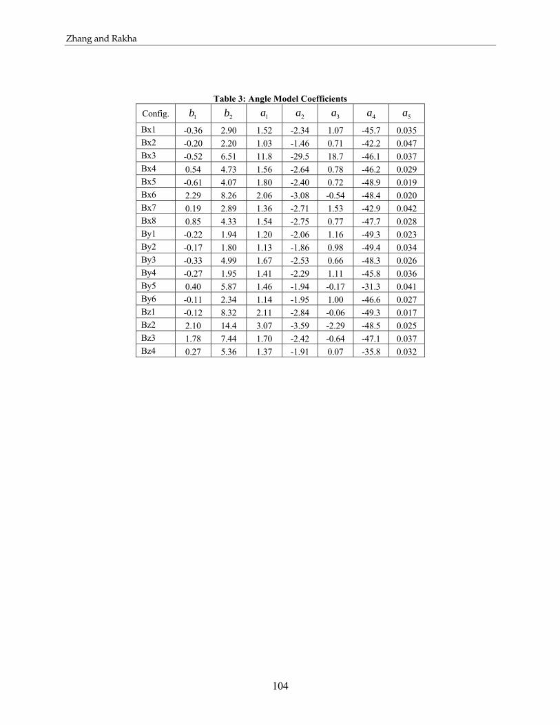
Zhang and Rakha

104

Table 3: Angle Model Coefficients Config. 1b 2b 1a 2a 3a 4a 5a

Bx1 -0.36 2.90 1.52 -2.34 1.07 -45.7 0.035 Bx2 -0.20 2.20 1.03 -1.46 0.71 -42.2 0.047 Bx3 -0.52 6.51 11.8 -29.5 18.7 -46.1 0.037 Bx4 0.54 4.73 1.56 -2.64 0.78 -46.2 0.029 Bx5 -0.61 4.07 1.80 -2.40 0.72 -48.9 0.019 Bx6 2.29 8.26 2.06 -3.08 -0.54 -48.4 0.020 Bx7 0.19 2.89 1.36 -2.71 1.53 -42.9 0.042 Bx8 0.85 4.33 1.54 -2.75 0.77 -47.7 0.028 By1 -0.22 1.94 1.20 -2.06 1.16 -49.3 0.023 By2 -0.17 1.80 1.13 -1.86 0.98 -49.4 0.034 By3 -0.33 4.99 1.67 -2.53 0.66 -48.3 0.026 By4 -0.27 1.95 1.41 -2.29 1.11 -45.8 0.036 By5 0.40 5.87 1.46 -1.94 -0.17 -31.3 0.041 By6 -0.11 2.34 1.14 -1.95 1.00 -46.6 0.027 Bz1 -0.12 8.32 2.11 -2.84 -0.06 -49.3 0.017 Bz2 2.10 14.4 3.07 -3.59 -2.29 -48.5 0.025 Bz3 1.78 7.44 1.70 -2.42 -0.64 -47.1 0.037 Bz4 0.27 5.36 1.37 -1.91 0.07 -35.8 0.032

Zhang and Rakha

105

Table 4: 95% Confidence Intervals for Angle Model Coefficients Config. 1b 2b 1a 2a 3a 4a 5a

Bx1 [-0.45 -0.27] [2.21 3.59] [1.19 1.85] [-2.88 -1.80] [0.83 1.31] [-56.8 -34.6] [0.03 0.04] Bx2 [-0.25 -0.15] [1.75 2.65] [0.77 1.29] [-1.82 -1.10] [0.52 0.90] [-52.7 -31.7] [0.03 0.06] Bx3 [-0.62 -0.42] [4.95 8.07] [8.68 14.9] [-35.9 -23.2] [14.4 23.0] [-55.4 -36.8] [0.03 0.04] Bx4 [0.46 0.62] [3.23 6.23] [1.24 1.88] [-3.07 -2.21] [0.62 0.94] [-55.1 -37.3] [0.02 0.04] Bx5 [-0.77 -0.45] [3.56 4.58] [1.69 1.91] [-2.73 -2.07] [0.65 0.77] [-50.3 – 47.5] [0.02 0.02] Bx6 [2.15 2.43] [6.50 10.02] [1.97 2.15] [-3.34 -2.82] [-0.65 -0.43] [-50.2 -46.6] [0.01 0.03] Bx7 [0.12 0. 26] [2.76 3.02] [1.12 1.60] [-2.95 – 2.47] [1.34 1.72] [-45.9 -39.9] [0.03 0.05] Bx8 [0.76 0.94] [3.98 4.68] [1.42 1.66] [-2.99 -2.51] [0.59 0.95] [-49.2 -46.2] [0.02 0.04] By1 [-0.27 -0.17] [1.50 2.38] [0.95 1.45] [-2.57 -1.55] [ 0.93 1.39] [-59.5 -39.1] [0.02 0.03] By2 [-0.21 -0.13] [1.42 2.18] [0.85 1.41] [-2.34 -1.38] [ 0.76 1.20] [-62.2 -36.6] [0.03 0.04] By3 [-0.41 -0.25] [3.97 6.01] [1.30 2.04] [-3.11 -1.95] [0.50 0.82] [-60.4 -36.2] [0.02 0.03] By4 [-0.34 -0.20] [1.55 2.35] [1.07 1.75] [-2.81 -1.77] [0.85 1.37] [-56.7 -34.9] [0.03 0.04] By5 [0.32 0.48] [4.57 7.17] [1.12 1.80] [-2.45 -1.43] [-0.20 -0.14] [-39.0 -23.6] [0.03 0.05] By6 [-0.14 -0.08] [1.72 2.96] [0.84 1.44] [-2.45 -1.45] [0.79 1.21] [-58.9 -34.3] [0.02 0.03] Bz1 [-0.15 -0.09] [6.11 10.5] [1.65 2.57] [-3.54 -2.14] [-0.08 -0.04] [-61.0 -37.6] [0.01 0.02] Bz2 [1.66 2.55] [11.0 17.8] [2.32 3.82] [-4.38 -2.80] [-2.80 -1.78] [-60.7 -36.3] [0.02 0.03] Bz3 [1.36 2.20] [5.46 9.42] [1.32 2.08] [-3.04 -1.80] [-0.77 -0.51] [-58.4 -35.8] [0.03 0.05] Bz4 [0.21 0.33] [4.04 6.68] [1.05 1.69] [-2.42 -1.40] [0.06 0.08] [-45.3 -26.3] [0.02 0.04]

Zhang and Rakha

106

Table 5: Effects of Random Seeds (Configuration Bx2) Random seed 100 200 300 400 500 600 700 800 900 average 0

MeRE 0.05 0.06 0.06 0.05 0.06 0.05 0.05 0.05 0.06 0.06 0.05 MaRE 0.22 0.22 0.21 0.22 0.22 0.22 0.23 0.21 0.21 0.22 0.20 MeAE 0.03 0.03 0.03 0.03 0.03 0.03 0.03 0.03 0.03 0.03 0.03 Model 1

MaAE 0.10 0.10 0.10 0.10 0.10 0.10 0.10 0.10 0.10 0.10 0.09 MeRE 0.04 0.04 0.04 0.04 0.05 0.05 0.04 0.04 0.04 0.04 0.04 MaRE 0.15 0.15 0.16 0.16 0.16 0.15 0.16 0.15 0.16 0.16 0.14 MeAE 0.02 0.02 0.02 0.02 0.02 0.02 0.02 0.02 0.02 0.02 0.02 Model 2

MaAE 0.12 0.13 0.12 0.12 0.13 0.12 0.13 0.12 0.12 0.12 0.11 MeRE 0.02 0.02 0.02 0.02 0.02 0.02 0.02 0.02 0.02 0.02 0.02 MaRE 0.10 0.09 0.10 0.10 0.10 0.10 0.10 0.09 0.10 0.10 0.09 MeAE 0.01 0.01 0.01 0.01 0.01 0.01 0.01 0.01 0.01 0.01 0.01 Model 3

MaAE 0.06 0.07 0.07 0.07 0.06 0.07 0.07 0.07 0.06 0.07 0.06 MeRE 0.05 0.06 0.05 0.06 0.05 0.06 0.05 0.05 0.06 0.05 0.05 MaRE 0.22 0.21 0.22 0.22 0.22 0.23 0.23 0.23 0.23 0.22 0.20 MeAE 0.03 0.03 0.03 0.03 0.03 0.03 0.03 0.03 0.03 0.03 0.03 Model 4

MaAE 0.13 0.13 0.13 0.13 0.13 0.13 0.13 0.13 0.14 0.13 0.12

Zhang and Rakha

107

Table 6: Differences between Simulation Results and Model Results Bx1 Bx2 Bx3 Bx4 Bx5 Bx6 Bx7 Bx8 By1 By2 By3 By4 By5 By6 Bz1 Bz2 Bz3 Bz4

MeRE 0.04 0.05 0.04 0.03 0.03 0.03 0.04 0.05 0.09 0.07 0.06 0.10 0.07 0.07 0.06 0.06 0.07 0.09MaRE 0.16 0.20 0.22 0.19 0.11 0.09 0.21 0.18 0.31 0.70 0.37 0.52 0.27 0.39 0.18 0.24 0.28 0.29MeAE 0.02 0.03 0.02 0.02 0.02 0.02 0.02 0.02 0.04 0.03 0.03 0.04 0.03 0.03 0.03 0.02 0.03 0.03

Model 1

MaAE 0.09 0.09 0.10 0.10 0.08 0.07 0.09 0.10 0.14 0.23 0.15 0.20 0.11 0.14 0.09 0.09 0.11 0.12MeRE 0.03 0.04 0.03 0.04 0.02 0.03 0.04 0.05 0.08 0.10 0.09 0.11 0.09 0.09 0.06 0.06 0.08 0.10MaRE 0.13 0.14 0.14 0.18 0.14 0.20 0.19 0.26 0.36 0.49 0.28 0.46 0.27 0.36 0.24 0.25 0.36 0.30MeAE 0.02 0.02 0.02 0.02 0.02 0.02 0.03 0.03 0.03 0.03 0.04 0.03 0.04 0.03 0.03 0.03 0.03 0.04

Model 2

MaAE 0.10 0.11 0.11 0.18 0.13 0.20 0.19 0.26 0.16 0.17 0.14 0.16 0.17 0.13 0.09 0.19 0.26 0.17MeRE 0.02 0.02 0.02 0.02 0.02 0.02 0.02 0.02 0.04 0.05 0.03 0.06 0.06 0.04 0.02 0.03 0.04 0.04MaRE 0.09 0.09 0.09 0.11 0.08 0.10 0.09 0.11 0.22 0.26 0.36 0.30 0.23 0.30 0.18 0.23 0.20 0.23MeAE 0.01 0.01 0.01 0.02 0.01 0.01 0.01 0.01 0.02 0.02 0.01 0.02 0.02 0.02 0.01 0.01 0.02 0.01

Model 3

MaAE 0.06 0.06 0.06 0.09 0.05 0.07 0.06 0.05 0.06 0.08 0.10 0.14 0.10 0.10 0.06 0.07 0.10 0.10MeRE 0.03 0.05 0.03 0.02 0.03 0.03 0.03 0.03 0.07 0.06 0.05 0.06 0.08 0.08 0.05 0.05 0.07 0.04MaRE 0.14 0.20 0.17 0.12 0.12 0.12 0.16 0.15 0.31 0.29 0.30 0.25 0.25 0.30 0.19 0.21 0.30 0.22MeAE 0.02 0.03 0.02 0.02 0.02 0.02 0.02 0.02 0.03 0.02 0.02 0.02 0.03 0.03 0.02 0.02 0.03 0.02

Model 4

MaAE 0.10 0.12 0.10 0.07 0.12 0.11 0.11 0.15 0.12 0.15 0.12 0.11 0.13 0.12 0.07 0.10 0.17 0.09MeRE 0.27 0.26 0.24 0.29 0.10 0.24 0.26 0.28 0.93 1.11 0.78 1.14 0.69 0.75 0.77 0.78 0.70 0.75MaRE 0.88 0.90 0.65 0.50 0.28 0.58 0.43 0.65 2.56 3.00 1.50 2.84 1.12 1.55 1.32 1.28 1.23 1.21MeAE 0.16 0.15 0.15 0.18 0.07 0.17 0.16 0.16 0.38 0.39 0.35 0.36 0.30 0.31 0.35 0.34 0.30 0.31

HCM

MaAE 0.42 0.44 0.38 0.32 0.23 0.38 0.28 0.39 0.66 0.67 0.58 0.68 0.52 0.60 0.48 0.49 0.51 0.52

Zhang and Rakha

108

Table 7: Statistics of Modelling Errors for 18 Type B Configurations Model Measure of Error Minimum Maximum Average

MeRE 0.03 0.10 0.06 MaRE 0.09 0.70 0.27 MeAE 0.02 0.04 0.03 Model 1

MaAE 0.07 0.23 0.12 MeRE 0.02 0.11 0.06 MaRE 0.13 0.49 0.26 MeAE 0.02 0.04 0.03 Model 2

MaAE 0.09 0.26 0.16 MeRE 0.02 0.06 0.03 MaRE 0.08 0.36 0.18 MeAE 0.01 0.02 0.01 Model 3

MaAE 0.05 0.14 0.08 MeRE 0.02 0.08 0.05 MaRE 0.12 0.31 0.21 MeAE 0.02 0.03 0.02 Model 4

MaAE 0.07 0.17 0.11 MeRE 0.10 1.14 0.57 MaRE 0.28 3.00 1.25 MeAE 0.07 0.39 0.26 HCM

MaAE 0.23 0.68 0.48

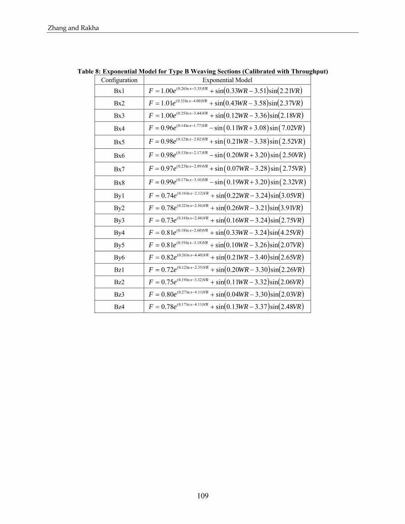
Zhang and Rakha

109

Table 8: Exponential Model for Type B Weaving Sections (Calibrated with Throughput) Configuration Exponential Model

Bx1 ( ) ( )VRWReF VRx 21.2sin51.333.0sin00.1 )35.3ln26.0( −+= −

Bx2 ( ) ( )VRWReF VRx 37.2sin58.343.0sin01.1 )00.4ln33.0( −+= −

Bx3 ( ) ( )VRWReF VRx 18.2sin36.312.0sin00.1 )44.3ln25.0( −+= −

Bx4 ( ) ( )(0.14ln 1.77)0.96 sin 0.11 3.08 sin 7.02x VRF e WR VR−= − +

Bx5 ( ) ( )(0.12ln 2.02)0.98 sin 0.21 3.38 sin 2.52x VRF e WR VR−= + −

Bx6 ( ) ( )(0.13ln 2.17)0.98 sin 0.20 3.20 sin 2.50x VRF e WR VR−= − +

Bx7 ( ) ( )(0.23ln 2.89)0.97 sin 0.07 3.28 sin 2.75x VRF e WR VR−= + −

Bx8 ( ) ( )(0.17ln 3.10)0.99 sin 0.19 3.20 sin 2.32x VRF e WR VR−= − +

By1 ( ) ( )VRWReF VRx 05.3sin24.322.0sin74.0 )12.2ln16.0( −+= −

By2 ( ) ( )VRWReF VRx 91.3sin21.326.0sin78.0 )56.2ln22.0( −+= −

By3 ( ) ( )VRWReF VRx 75.2sin24.316.0sin73.0 )44.2ln16.0( −+= −

By4 ( ) ( )VRWReF VRx 25.4sin24.333.0sin81.0 )60.2ln18.0( −+= −

By5 ( ) ( )VRWReF VRx 07.2sin26.310.0sin81.0 )18.3ln19.0( −+= −

By6 ( ) ( )VRWReF VRx 65.2sin40.321.0sin82.0 )40.4ln26.0( −+= −

Bz1 ( ) ( )VRWReF VRx 26.2sin30.320.0sin72.0 )35.2ln12.0( −+= −

Bz2 ( ) ( )VRWReF VRx 06.2sin32.311.0sin75.0 )32.3ln19.0( −+= −

Bz3 ( ) ( )VRWReF VRx 03.2sin30.304.0sin80.0 )11.4ln27.0( −+= −

Bz4 ( ) ( )VRWReF VRx 48.2sin37.313.0sin78.0 )11.4ln17.0( −+= −

Zhang and Rakha

110

Table 9: Angle Model Coefficients (Calibrated with Throughput) Config. 1b 2b 1a 2a 3a 4a 5a

Bx1 -0.05 1.91 0.67 -1.27 0.83 -42.3 0.045 Bx2 -0.02 1.66 0.42 -1.02 0.75 -34.8 0.057 Bx3 -0.02 1.66 0.42 -1.02 0.75 -34.8 0.057 Bx4 0.32 2.88 0.54 -0.32 -0.22 -45.3 0.032 Bx5 -0.19 2.59 0.62 -0.26 -0.08 -48.8 0.019 Bx6 0.85 3.34 0.54 -0.38 -0.32 -47.9 0.022 Bx7 0.11 2.82 0.56 -0.31 -0.22 -41.7 0.046 Bx8 0.39 2.10 0.47 -0.49 0.11 -46.6 0.029 By1 -0.13 2.23 0.51 -1.25 0.70 -47.7 0.036 By2 -0.10 2.08 1.24 -1.68 0.71 -49.3 0.053 By3 -0.46 4.62 7.25 -5.22 1.13 -49.2 0.034 By4 -0.05 1.76 1.07 -1.47 0.64 -25.4 0.066 By5 -0.07 4.43 10.0 -4.72 0.75 -46.9 0.035 By6 -0.27 3.18 5.03 -3.98 0.99 -45.9 0.037 Bz1 -0.14 2.81 2.57 -2.33 0.78 -47.9 0.019 Bz2 -0.01 4.26 7.52 -3.53 0.65 -46.4 0.025 Bz3 0.41 27.3 422.4 -14.0 0.32 -45.4 0.034 Bz4 -0.23 4.97 12.45 -5.64 0.85 9.3 0.034

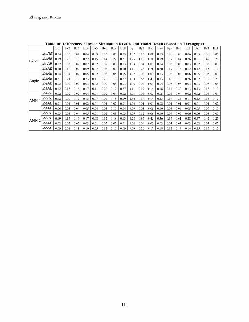
Zhang and Rakha

111

Table 10: Differences between Simulation Results and Model Results Based on Throughput Bx1 Bx2 Bx3 Bx4 Bx5 Bx6 Bx7 Bx8 By1 By2 By3 By4 By5 By6 Bz1 Bz2 Bz3 Bz4

MeRE 0.04 0.05 0.04 0.04 0.03 0.03 0.05 0.05 0.07 0.13 0.08 0.13 0.08 0.08 0.06 0.05 0.08 0.06 MaRE 0.19 0.26 0.20 0.22 0.15 0.14 0.27 0.21 0.26 1.10 0.70 0.79 0.37 0.84 0.26 0.31 0.42 0.26 MeAE 0.02 0.03 0.02 0.02 0.02 0.02 0.03 0.03 0.03 0.04 0.03 0.04 0.03 0.03 0.03 0.02 0.03 0.03

Expo.

MaAE 0.10 0.10 0.09 0.09 0.07 0.08 0.09 0.10 0.11 0.28 0.26 0.20 0.17 0.26 0.12 0.12 0.15 0.14 MeRE 0.04 0.04 0.04 0.05 0.02 0.03 0.05 0.05 0.07 0.06 0.07 0.13 0.06 0.08 0.06 0.05 0.05 0.06 MaRE 0.21 0.21 0.19 0.23 0.11 0.20 0.19 0.27 0.30 0.65 0.43 0.73 0.40 0.70 0.26 0.32 0.32 0.26 MeAE 0.02 0.02 0.02 0.03 0.02 0.02 0.03 0.03 0.03 0.04 0.03 0.04 0.03 0.03 0.03 0.03 0.03 0.03

Angle

MaAE 0.12 0.13 0.16 0.17 0.11 0.20 0.19 0.27 0.11 0.19 0.14 0.18 0.14 0.22 0.13 0.13 0.13 0.12 MeRE 0.02 0.02 0.02 0.04 0.01 0.02 0.04 0.02 0.05 0.03 0.03 0.05 0.03 0.04 0.02 0.02 0.03 0.04 MaRE 0.12 0.09 0.12 0.13 0.07 0.07 0.13 0.09 0.30 0.16 0.14 0.23 0.16 0.25 0.11 0.15 0.15 0.17 MeAE 0.01 0.01 0.01 0.02 0.01 0.01 0.02 0.01 0.02 0.01 0.01 0.02 0.01 0.01 0.01 0.01 0.01 0.02

ANN 1

MaAE 0.06 0.05 0.04 0.05 0.04 0.05 0.10 0.04 0.09 0.05 0.05 0.10 0.08 0.06 0.05 0.05 0.07 0.10 MeRE 0.03 0.03 0.04 0.05 0.01 0.02 0.03 0.03 0.05 0.12 0.06 0.10 0.07 0.07 0.06 0.06 0.08 0.05 MaRE 0.19 0.17 0.16 0.17 0.08 0.12 0.18 0.13 0.28 0.87 0.45 0.56 0.37 0.61 0.28 0.37 0.42 0.25 MeAE 0.02 0.02 0.02 0.03 0.01 0.02 0.02 0.01 0.02 0.04 0.03 0.03 0.03 0.03 0.03 0.02 0.03 0.02

ANN 2

MaAE 0.09 0.08 0.11 0.10 0.05 0.12 0.10 0.09 0.09 0.26 0.17 0.18 0.12 0.19 0.14 0.15 0.15 0.15

Zhang and Rakha

112

Table 11: Statistics of Modelling Errors Based on Throughput for Type B Configurations Model Measure of Error Minimum Maximum Average

MeRE 0.04 0.13 0.07 MaRE 0.19 1.10 0.46 MeAE 0.02 0.04 0.03 Expo.

MaAE 0.09 0.28 0.16 MeRE 0.02 0.13 0.06 MaRE 0.11 0.73 0.33 MeAE 0.02 0.04 0.03 Angle

MaAE 0.11 0.27 0.16 MeRE 0.01 0.05 0.03 MaRE 0.07 0.3 0.15 MeAE 0.01 0.02 0.01 ANN 1

MaAE 0.04 0.1 0.06 MeRE 0.01 0.12 0.05 MaRE 0.08 0.87 0.31 MeAE 0.01 0.04 0.02 ANN 2

MaAE 0.05 0.26 0.13

Zhang and Rakha

113

Bx1

Bx2

Bx3

Bx4

Bx5

Bx6

Bx7

Bx8

By1

By2

By3

By4

By5

By6

Bz1

Bz2

Bz3 Bz4

Figure 1: Configurations of Type B Weaving Sections

Zhang and Rakha

114

0% 20% 40% 60% 80% 100%0.000.100.20

0.300.400.500.600.700.80

0.901.001.10

Volume Ratio

Cap

acity

Fac

tor

SimulationHCM

Length of Core Weaving Area = 150 m

0% 20% 40% 60% 80% 100%0.000.100.20

0.300.400.500.600.700.80

0.901.001.10

Volume Ratio

Capa

city

Fac

tor

SimulationHCM

Length of Core Weaving Area = 450 m

0% 20% 40% 60% 80% 100%0.000.100.20

0.300.400.500.600.700.80

0.901.001.10

Volume Ratio

Capa

city

Fac

tor

SimulationHCM

Length of Core Weaving Area = 750 m

Figure 2: Simulation Results and Results from HCM Procedures (Bx2)

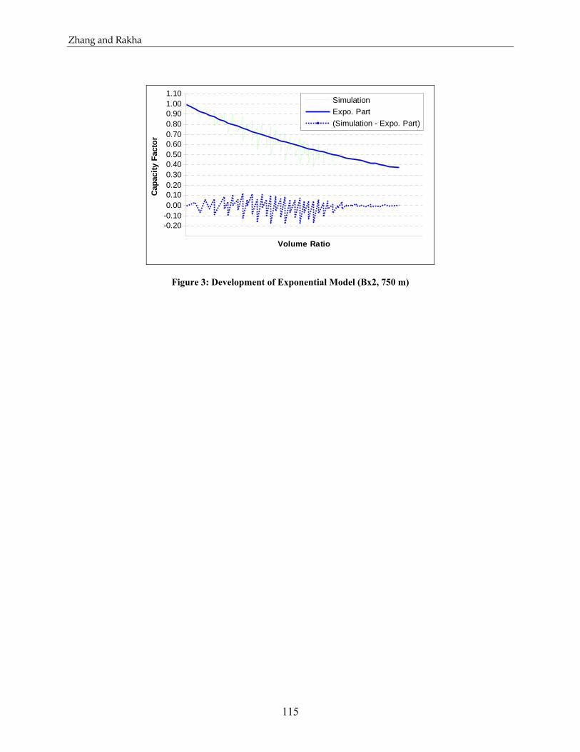
Zhang and Rakha

115

-0.20-0.100.000.100.200.300.400.500.600.700.800.901.001.10

Volume Ratio

Capa

city

Fac

tor

SimulationExpo. Part(Simulation - Expo. Part)

Figure 3: Development of Exponential Model (Bx2, 750 m)

Zhang and Rakha

116

0.30.4

0.40.5

0.50.6

0.60.7

0.70.7

0.80.8

0.8

0.9

VR

WR

0 0.2 0.4 0.6 0.80

0.2

0.4

0.6

0.8

1

50 m

0.3

0.4

0.4

0.4

0.40.40.4

0.4

0.4

0.4

0.4

0.4

0.4

0.4

0.4

0.4

0.40.4

0.40.4

0.4

0.4

0.4

0.40.4

0.4

0.4

0.4 0.4

0.4

0.40.4

0.4

0.4

0.4

0.4

0.40.4

0.40.4

0.4

0.40.50.5

0.5

0.5

0.50.5

0.50.5

0.5

0.50.5

0.5

0.50.5

0.50.5

0.5

0.50.5

0.50.5

0.5

0.5

0.50.5 0.5

0.5

0.5

0.5

0.5

0.50.5

0.50.5

0.5

0.5

0.50.5

0.5

0.50.5

0.5

0.50.5

0.5 0.50.5

0.50.5

0.50.5

0.5

0.5 0.5

0.50.5

0.5

0.60.6

0.6

0.60.6

0.6

0.60.6

0.6

0.6

0.6

0.60.60.6 0.60.6

0.6

0.6

0.60.6

0.60.6

0.60.6

0.6

0.6

0.60.6

0.6

0.6

0.60.6

0.6

0.60.6

0.60.6 0.6

0.60.60.60.6

0.6

0.60.6

0.7

0.7

0.7

0.70.7

0.7

0.7

0.70.7

0.70.7

0.70.7

0.7

0.70.7

0.7

0.70.7

0.7

0.70.7

0.7

0.7

0.70.7

0.7

0.7

0.8

0.8

0.80.8

0.8

0.8

0.80.8

0.80.8

0.80.80.8

0.80.8

0.9

0.9

VR

WR

0.2 0.4 0.6 0.80

0.1

0.2

0.3

0.4

0.5

0.6

0.7

0.8

150 m

0.4

0.40.4

0.4

0.40.4

0.4

0.4

0.4

0.40.4

0.40.40.4

0.40.40.40.4

0.40.4

0.4

0.4

0.4

0.4

0.4

0.4

0.40.4 0.40.40.4

0.40.40.5

0.5

0.5 0.50.5

0.50.50.5

0.50.5

0.50.5

0.5

0.50.5

0.5

0.50.5

0.50.5

0.50.5

0.5

0.5

0.5

0.5

0.5

0.5

0.50.5

0.5

0.50.5

0.5

0.5

0.5

0.50.5

0.5 0.5

0.5

0.5

0.50.5

0.50.5

0.50.5

0.5

0.5

0.5

0.5

0.50.5

0.5

0.5 0.50.5

0.5

0.5 0.5

0.60.6

0.60.6

0.60.60.60.6

0.60.60.6

0.6

0.60.6 0.6

0.6

0.60.6

0.6

0.6

0.60.6

0.60.6 0.6 0.60.60.6

0.60.6

0.60.6

0.60.6

0.60.60.60.6

0.6

0.60.6

0.6

0.6

0.6

0.60.6

0.6

0.60.6

0.6

0.60.6 0.6

0.60.6

0.60.60.6

0.7

0.7

0.70.7

0.70.7

0.7

0.7

0.70.70.7

0.70.70.7

0.7

0.70.7

0.7

0.7

0.70.7

0.7

0.7

0.7

0.7

0.70.7

0.7

0.7

0.70.7

0.70.7

0.70.7

0.70.7

0.7

0.7

0.7

0.70.7

0.70.8

0.8

0.80.8

0.80.8

0.80.80.8

0.8

0.80.8

0.80.8

0.8

0.80.8

0.8

0.80.8

0.80.90.9

0.9

0.90.9

VR

WR

0.2 0.4 0.6 0.80

0.1

0.2

0.3

0.4

0.5

0.6

0.7

0.8

450 m

0.4

0.4

0.4

0.4

0.40.4

0.4

0.4

0.4

0.4

0.4

0.4

0.40.4

0.4

0.4

0.4

0.4

0.5

0.5

0.5

0.50.5

0.50.5

0.5

0.5

0.50.5

0.50.5 0.5

0.5

0.5

0.5

0.50.5

0.5

0.50.5

0.5

0.5

0.5

0.5 0.5

0.6

0.6

0.6

0.60.6

0.60.6

0.60.6

0.6 0.6

0.6

0.6

0.6

0.60.6

0.6

0.6

0.60.6

0.60.6

0.60.6

0.6

0.60.6

0.7

0.7

0.7

0.7

0.7

0.70.7

0.70.7

0.7

0.7

0.7

0.7

0.7

0.7

0.7

0.70.7

0.7

0.7 0.70.70.7

0.7

0.7

0.70.7

0.70.8

0.8

0.8

0.8

0.80.8

0.8

0.80.8

0.80.8

0.8

0.80.8

0.8

0.80.8

0.8

0.8

0.80.8

0.90.90.90.9 0.9

0.9

VR

WR

0.2 0.4 0.6 0.80

0.1

0.2

0.3

0.4

0.5

0.6

0.7

0.8

750 m

Figure 4: Contour Plots of Capacity Factor

Zhang and Rakha

117

0.4

0.4

0.4

0.4

0.40.4

0.4

0.4

0.4

0.4

0.4

0.4

0.40.4

0.4

0.4

0.4

0.4

0.5

0.5

0.5

0.50.5

0.50.5

0.5

0.50.5

0.50.5

0.5 0.5

0.5

0.5

0.5

0.50.5

0.5

0.50.5

0.5

0.5

0.5

0.5 0.5

0.6

0.6

0.60.6

0.6

0.60.6

0.60.6

0.6 0.6

0.6

0.6

0.6

0.60.6

0.6

0.6

0.60.6

0.60.6

0.60.6

0.6

0.60.6

0.7

0.7

0.70.7

0.7

0.70.7

0.70.70.7

0.7

0.70.7

0.7

0.7

0.7

0.70.7

0.7

0.7 0.70.70.7

0.7

0.7

0.70.7

0.70.8

08

0.8

08

0.80.8

0.8

0.80.8

0.80.8

0.8

0.80.8

0.8

0.80.8

0.8

0.8

0.80.8

0.90.90.90

9 0.90.9

VR

WR

0.2 0.4 0.6 0.80

0.1

0.2

0.3

0.4

0.5

0.6

0.7

0.8

P0 (b1, b2)

θ

P1 (VR1, WR1)

Figure 5: Definition of θ

Zhang and Rakha

118

y = 0.4983x2 - 0.1976x + 0.1092R2 = 0.9398

0.2

0.3

0.4

0.5

0.6

0.7

0.8

0.9

1

1.1

0.8 1 1.2 1.4 1.6 1.8

theta

Cap

acity

Fac

tor

Figure 6: Relationship between Capacity Factor and θ

Zhang and Rakha

119

Volume Percentage of FR

Volume Percentage of RF

Volume Percentage of RR

Weaving Section Length

F

Volume Percentage of FF

Figure 7: Structure of ANN Model 1

Zhang and Rakha

120

Volume Ratio

Weaving Ratio

Weaving Section Length

F

Figure 8: Structure of ANN Model 2

Zhang and Rakha

121

0% 20% 40% 60% 80% 100%0.000.100.20

0.300.400.500.600.700.80

0.901.001.10

Volume Ratio

Capa

city

Fac

tor

SimulationExponential ModelHCM

0% 20% 40% 60% 80% 100%

0.000.100.20

0.300.400.500.600.700.80

0.901.001.10

Volume Ratio

Capa

city

Fac

tor

SimulationAngle ModelHCM

0% 20% 40% 60% 80% 100%0.000.100.20

0.300.400.500.600.700.80

0.901.001.10

Volume Ratio

Capa

city

Fac

tor

SimulationANN Model 1HCM

0% 20% 40% 60% 80% 100%

0.000.100.20

0.300.400.500.600.700.80

0.901.001.10

Volume Ratio

Capa

city

Fac

tor

SimulationANN Model 2HCM

Figure 9: Comparison of Model Results, Simulation Results, and HCM Results (Bx2, 300 m)

Zhang and Rakha

122

1 2 3 4 5 6 7 8 9 100.40

0.50

0.60

0.70

0.80

0.90

1.00

1.10

Days

Cap

acity

Fac

tor

Expo. ModelField

Exponential Model

1 2 3 4 5 6 7 8 9 100.40

0.50

0.60

0.70

0.80

0.90

1.00

1.10

Days

Cap

acity

Fac

tor

Angle ModelField

Angle Model

1 2 3 4 5 6 7 8 9 100.40

0.50

0.60

0.70

0.80

0.90

1.00

1.10

Days

Cap

acity

Fac

tor

ANN Model 1Field

ANN Model 1

1 2 3 4 5 6 7 8 9 100.40

0.50

0.60

0.70

0.80

0.90

1.00

1.10

Days

Cap

acity

Fac

tor

ANN Model 2Field

ANN Model 2

1 2 3 4 5 6 7 8 9 100.40

0.50

0.60

0.70

0.80

0.90

1.00

1.10

Days

Cap

acity

Fac

tor

HCMField

HCM

Figure 10: Model Validation with Field Data (Bx4)

Zhang and Rakha

123

Expo. Model Angle Model

ANN Model 1 ANN Model 2

HCM

0.0

0.2

0.4

0.6

0.8

1.0

50 150 250 350 450 550 650 750

Weaving Section Length (m)

Cap

acity

Fac

tor

VR = 0.0 VR = 0.2VR = 0.4 VR = 0.6VR = 0.8 VR = 1.0

0.0

0.2

0.4

0.6

0.8

1.0

50 150 250 350 450 550 650 750Weaving Section Length (m)

Cap

acity

Fac

tor

VR = 0.0 VR = 0.2VR = 0.4 VR = 0.6VR = 0.8 VR = 1.0

0.0

0.2

0.4

0.6

0.8

1.0

50 150 250 350 450 550 650 750Weaving Section Length (m)

Cap

acity

Fac

tor

VR = 0.0 VR = 0.2VR = 0.4 VR = 0.6VR = 0.8 VR = 1.0

0.0

0.2

0.4

0.6

0.8

1.0

50 150 250 350 450 550 650 750Weaving Section Length (m)

Cap

acity

Fac

tor

VR = 0.0 VR = 0.2VR = 0.4 VR = 0.6VR = 0.8 VR = 1.0

0.0

0.2

0.4

0.6

0.8

1.0

50 150 250 350 450 550 650 750Weaving Section Length (m)

Cap

acity

Fac

tor

VR = 0.0 VR = 0.2VR = 0.4 VR = 0.6VR = 0.8 VR = 1.0

Figure 11: Weaving Section Length ~ Capacity Factor Relationship in HCM (Bx2, WR = 0.5)

Zhang and Rakha

124

Expo. Model Angle Model

ANN Model 1 ANN Model 2

HCM

0.0

0.2

0.4

0.6

0.8

1.0

0 0.2 0.4 0.6 0.8 1

VR

Cap

acity

Fac

tor

WR = 0.0 WR = 0.2WR = 0.4 WR = 0.6WR = 0.8 WR = 1.0

0.0

0.2

0.4

0.6

0.8

1.0

0 0.2 0.4 0.6 0.8 1VR

Cap

acity

Fac

tor

WR = 0.0 WR = 0.2WR = 0.4 WR = 0.6WR = 0.8 WR = 1.0

0.0

0.2

0.4

0.6

0.8

1.0

0 0.2 0.4 0.6 0.8 1VR

Cap

acity

Fac

tor

WR = 0.0 WR = 0.2WR = 0.4 WR = 0.6WR = 0.8 WR = 1.0

0.0

0.2

0.4

0.6

0.8

1.0

0 0.2 0.4 0.6 0.8 1VR

Cap

acity

Fac

tor

WR = 0.0 WR = 0.2WR = 0.4 WR = 0.6WR = 0.8 WR = 1.0

0.0

0.2

0.4

0.6

0.8

1.0

0 0.2 0.4 0.6 0.8 1VR

Cap

acity

Fac

tor

WR = 0.0 WR = 0.2WR = 0.4 WR = 0.6WR = 0.8 WR = 1.0

Figure 12: Volume Ratio ~ Capacity Factor Relationship in HCM (Bx2, 300 m)

Zhang and Rakha

125

0 0.2 0.4 0.6 0.8 10

0.2

0.4

0.6

0.8

1

Volume Ratio

Wea

ving

Rat

io

Bx1

0 0.2 0.4 0.6 0.8 10

0.2

0.4

0.6

0.8

1

Volume RatioW

eavi

ng R

atio

Bx2

0 0.2 0.4 0.6 0.8 10

0.2

0.4

0.6

0.8

1

Volume Ratio

Wea

ving

Rat

io

Bx3

0 0.2 0.4 0.6 0.8 10

0.2

0.4

0.6

0.8

1

Volume Ratio

Wea

ving

Rat

io

Bx4

0 0.2 0.4 0.6 0.8 10

0.2

0.4

0.6

0.8

1

Volume Ratio

Wea

ving

Rat

io

Bx5

0 0.2 0.4 0.6 0.8 10

0.2

0.4

0.6

0.8

1

Volume Ratio

Wea

ving

Rat

io

Bx6

0 0.2 0.4 0.6 0.8 10

0.2

0.4

0.6

0.8

1

Volume RatioW

eavi

ng R

atio

Bx7

0 0.2 0.4 0.6 0.8 10

0.2

0.4

0.6

0.8

1

Volume Ratio

Wea

ving

Rat

io

Bx8

0 0.2 0.4 0.6 0.8 10

0.2

0.4

0.6

0.8

1

Volume Ratio

Wea

ving

Rat

io

By1

0 0.2 0.4 0.6 0.8 10

0.2

0.4

0.6

0.8

1

Volume Ratio

Wea

ving

Rat

io

By2

0 0.2 0.4 0.6 0.8 10

0.2

0.4

0.6

0.8

1

Volume Ratio

Wea

ving

Rat

io

By3

0 0.2 0.4 0.6 0.8 10

0.2

0.4

0.6

0.8

1

Volume RatioW

eavi

ng R

atio

By4

0 0.2 0.4 0.6 0.8 10

0.2

0.4

0.6

0.8

1

Volume Ratio

Wea

ving

Rat

io

By5

0 0.2 0.4 0.6 0.8 10

0.2

0.4

0.6

0.8

1

Volume Ratio

Wea

ving

Rat

io

By6

0 0.2 0.4 0.6 0.8 10

0.2

0.4

0.6

0.8

1

Volume Ratio

Wea

ving

Rat

io

Bz1

0 0.2 0.4 0.6 0.8 10

0.2

0.4

0.6

0.8

1

Volume Ratio

Wea

ving

Rat

io

Bz2

0 0.2 0.4 0.6 0.8 10

0.2

0.4

0.6

0.8

1

Volume Ratio

Wea

ving

Rat

io

Bz3

0 0.2 0.4 0.6 0.8 10

0.2

0.4

0.6

0.8

1

Volume Ratio

Wea

ving

Rat

io

Bz4

Figure 13: Distribution of Simulated Data Points in VR-WR Plane (Demand)

Zhang and Rakha

126

0 0.2 0.4 0.6 0.8 10

0.2

0.4

0.6

0.8

1

Volume Ratio

Wea

ving

Rat

io

demandthroughput

Figure 14: Comparing throughput and demand (Configuration Bx2, 450 m)

Zhang and Rakha

127

0 0.2 0.4 0.6 0.8 10

0.2

0.4

0.6

0.8

1

Volume Ratio

Wea

ving

Rat

io

Bx1

0 0.2 0.4 0.6 0.8 10

0.2

0.4

0.6

0.8

1

Volume RatioW

eavi

ng R

atio

Bx2

0 0.2 0.4 0.6 0.8 10

0.2

0.4

0.6

0.8

1

Volume Ratio

Wea

ving

Rat

io

Bx3

0 0.2 0.4 0.6 0.8 10

0.2

0.4

0.6

0.8

1

Volume Ratio

Wea

ving

Rat

io

Bx4

0 0.2 0.4 0.6 0.8 10

0.2

0.4

0.6

0.8

1

Volume Ratio

Wea

ving

Rat

io

Bx5

0 0.2 0.4 0.6 0.8 10

0.2

0.4

0.6

0.8

1

Volume Ratio

Wea

ving

Rat

io

Bx6

0 0.2 0.4 0.6 0.8 10

0.2

0.4

0.6

0.8

1

Volume RatioW

eavi

ng R

atio

Bx7

0 0.2 0.4 0.6 0.8 10

0.2

0.4

0.6

0.8

1

Volume Ratio

Wea

ving

Rat

io

Bx8

0 0.2 0.4 0.6 0.8 10

0.2

0.4

0.6

0.8

1

Volume Ratio

Wea

ving

Rat

io

By1

0 0.2 0.4 0.6 0.8 10

0.2

0.4

0.6

0.8

1

Volume Ratio

Wea

ving

Rat

io

By2

0 0.2 0.4 0.6 0.8 10

0.2

0.4

0.6

0.8

1

Volume Ratio

Wea

ving

Rat

io

By3

0 0.2 0.4 0.6 0.8 10

0.2

0.4

0.6

0.8

1

Volume Ratio

Wea

ving

Rat

io

By4

0 0.2 0.4 0.6 0.8 10

0.2

0.4

0.6

0.8

1

Volume Ratio

Wea

ving

Rat

io

By5

0 0.2 0.4 0.6 0.8 10

0.2

0.4

0.6

0.8

1

Volume Ratio

Wea

ving

Rat

io

By6

0 0.2 0.4 0.6 0.8 10

0.2

0.4

0.6

0.8

1

Volume Ratio

Wea

ving

Rat

io

Bz1

0 0.2 0.4 0.6 0.8 10

0.2

0.4

0.6

0.8

1

Volume Ratio

Wea

ving

Rat

io

Bz2

0 0.2 0.4 0.6 0.8 10

0.2

0.4

0.6

0.8

1

Volume Ratio

Wea

ving

Rat

io

Bz3

0 0.2 0.4 0.6 0.8 10

0.2

0.4

0.6

0.8

1

Volume Ratio

Wea

ving

Rat

io

Bz4

Figure 15: Distribution of Simulated Data Points in VR-WR Plane (Throughput)

Zhang and Rakha

128

Expo. Model Angle Model

ANN Model 1 ANN Model 2

HCM

0.0

0.2

0.4

0.6

0.8

1.0

0 0.2 0.4 0.6 0.8 1

VR

Cap

acity

Fac

tor

WR = 0.0 WR = 0.2WR = 0.4 WR = 0.6WR = 0.8 WR = 1.0

0.0

0.2

0.4

0.6

0.8

1.0

0 0.2 0.4 0.6 0.8 1VR

Cap

acity

Fac

tor

WR = 0.0 WR = 0.2WR = 0.4 WR = 0.6WR = 0.8 WR = 1.0

0.0

0.2

0.4

0.6

0.8

1.0

0 0.2 0.4 0.6 0.8 1VR

Cap

acity

Fac

tor

WR = 0.0 WR = 0.2WR = 0.4 WR = 0.6WR = 0.8 WR = 1.0

0.0

0.2

0.4

0.6

0.8

1.0

0 0.2 0.4 0.6 0.8 1VR

Cap

acity

Fac

tor

WR = 0.0 WR = 0.2WR = 0.4 WR = 0.6WR = 0.8 WR = 1.0

0.0

0.2

0.4

0.6

0.8

1.0

0 0.2 0.4 0.6 0.8 1VR

Cap

acity

Fac

tor

WR = 0.0 WR = 0.2WR = 0.4 WR = 0.6WR = 0.8 WR = 1.0

Figure 16: Impact of Volume Ratio on Capacity Factor Excluding Points right to the Curves in Figure 13

Zhang and Rakha

129

APPENDIX 1: EXAMPLE PROBLEM

In the following the procedures for applying all the models proposed in this paper are illustrated.

The Weaving Section A weaving section as shown below.

700

150

500250

D

C A

B

The Question What is the capacity of this weaving section? The Facts Volume (A-C) = 700 veh/h Volume (A-D) = 500 veh/h Volume (B-C) = 150 veh/h Volume (B-D) = 250 veh/h 15 percent trucks PHF = 0.85 Rolling terrrian Drivers are regular commuters FFS = 100 km/h for freeway Capacity of 2,000 pc/h for on-ramp Weaving section length = 300 m

Zhang and Rakha

130

Steps by exponential model 1. Convert volume (veh/h) to flow rate(pc/h) ( )( )( )HV p

VvPHF f f

=

700(A-C) 1,009 pc/h(0.85)(0.816)(1.0)

v = =

(A-D) 721 pc/hv = (B-C) 216 pc/hv = (B-D) 360 pc/hv =

1a. Determine pf 1.0pf = 1b. Determine HVf 1

1 ( 1) ( 1)HVT T R R

fP E P E

=+ − + −

1 0.8161 0.15(2.5 1)HVf = =+ −

2. Decide configuration type

Bx4

3. Compute critical variables

721 216 937 pc/hwv = + = 1,009 360 1,369 pc/hnwv = + =

937 1,369 2,306 pc/hv = + = 937 0.406

2,306VR = =

721 0.769937

WR = = (different definition from HCM)

4. Compute capacity factor ( ) ( )(0.14ln 1.77)0.96 sin 0.11 3.08 sin 7.02x VRF e WR VR−= − +

( ) ( )(0.14ln(300) 1.77)(0.406)0.96 sin 0.11 0.769 3.08 sin 7.02 0.406F e −= − ⋅ + ⋅

( ) ( )0.3940.96 sin 3.165 sin 2.85F e−= −

( )0.96 0.674 (0.055) 0.050F = ⋅ − 0.644F =

5. Compute incoming capacity

incoming (2,300)(3) 2,000 8,900 pc/hC = + =

6. Compute capacity incomingCapacity (0.644)(8,900) 5,734 pc/hF C= ⋅ = =

Zhang and Rakha

131

Steps by angle model 1. Convert volume (veh/h) to flow rate(pc/h) ( )( )( )HV p

VvPHF f f

=

700(A-C) 1,009 pc/h(0.85)(0.816)(1.0)

v = =

(A-D) 721 pc/hv = (B-C) 216 pc/hv = (B-D) 360 pc/hv =

1a. Determine pf 1.0pf = 1b. Determine HVf 1

1 ( 1) ( 1)HVT T R R

fP E P E

=+ − + −

1 0.8161 0.15(2.5 1)HVf = =+ −

2. Decide configuration type

Bx4

3. Compute critical variables

721 216 937 pc/hwv = + = 1,009 360 1,369 pc/hnwv = + =

937 1,369 2,306 pc/hv = + = 937 0.406

2,306VR = =

721 0.769937

WR = = (different definition from HCM)

4. Compute capacity factor 1 1

2 21 2

cos( ) ( )

VR b

VR b b WRθ −

⎛ ⎞⎟−⎜ ⎟⎜= ⎟⎜ ⎟⎜ ⎟⎟⎜ − + −⎝ ⎠

1

2 2

1

0.406 0.54cos

(0.406 0.54) (4.73 0.769)

0.134 cos 1.605

3.963

θ −

−

⎛ ⎞⎟−⎜ ⎟⎜= ⎟⎜ ⎟⎜ ⎟⎟⎜ − + −⎝ ⎠

⎛− ⎞⎟⎜= =⎟⎜ ⎟⎜⎝ ⎠

( ) 521 2 3 4( )aF a a a x aθ θ= + + +

( )2 0.0291.56 1.605 2.64 1.605 0.78 (300 46.2)F = ⋅ − ⋅ + − (0.561)(1.174) 0.659F = =

5. Compute incoming capacity

incoming (2,300)(3) 2,000 8,900 pc/hC = + =

6. Compute capacity incomingCapacity (0.659)(8,900) 5,866 pc/hF C= ⋅ = =

Zhang and Rakha

132

Steps by ANN model 1 1. Convert volume (veh/h) to flow rate(pc/h) ( )( )( )HV p

VvPHF f f

=

700(A-C) 1,009 pc/h(0.85)(0.816)(1.0)

v = =

(A-D) 721 pc/hv = (B-C) 216 pc/hv = (B-D) 360 pc/hv =

1a. Determine pf 1.0pf = 1b. Determine HVf 1

1 ( 1) ( 1)HVT T R R

fP E P E

=+ − + −

1 0.8161 0.15(2.5 1)HVf = =+ −

2. Decide configuration type

Bx4

3. Compute critical variables

721 216 937 pc/hwv = + = 1,009 360 1,369 pc/hnwv = + =

937 1,369 2,306 pc/hv = + = 1,009 0.4382,306

FF = =

721 0.3132,306

FR = =

216 0.09372,306

RF = =

360 0.1562,306

RR = =

4. Compute capacity factor

))(tan(log 21 bbpIWsigLWsigF ++⋅⋅= Substitute p with value of (300, 0.438, 0.313, 0.0937, 0.156)’, and substitute the other coefficients with the corresponding values shown in Appendix 2,

0.639F = 5. Compute incoming capacity

incoming (2,300)(3) 2,000 8,900 pc/hC = + =

6. Compute capacity incomingCapacity (0.639)(8,900) 5,688 pc/hF C= ⋅ = =

Zhang and Rakha

133

Steps by ANN model 2 1. Convert volume (veh/h) to flow rate(pc/h) ( )( )( )HV p

VvPHF f f

=

700(A-C) 1,009 pc/h(0.85)(0.816)(1.0)

v = =

(A-D) 721 pc/hv = (B-C) 216 pc/hv = (B-D) 360 pc/hv =

1a. Determine pf 1.0pf = 1b. Determine HVf 1

1 ( 1) ( 1)HVT T R R

fP E P E

=+ − + −

1 0.8161 0.15(2.5 1)HVf = =+ −

2. Decide configuration type

Bx4

3. Compute critical variables

721 216 937 pc/hwv = + = 1,009 360 1,369 pc/hnwv = + =

937 1,369 2,306 pc/hv = + = 937 0.406

2,306VR = =

721 0.769937

WR = = (different definition from HCM)

4. Compute capacity factor

))(tan(log 21 bbpIWsigLWsigF ++⋅⋅= Substitute p with value of (300, 0.406, 0.769)’, and substitute the other coefficients with the corresponding values shown in Appendix 3,

0.675F = 5. Compute incoming capacity

incoming (2,300)(3) 2,000 8,900 pc/hC = + =

6. Compute capacity incomingCapacity (0.675)(8,900) 6,011 pc/hF C= ⋅ = =

Zhang and Rakha

134

Steps by HCM 2000 Procedures 1. Convert volume (veh/h) to flow rate(pc/h) ( )( )( )HV p

VvPHF f f

=

700(A-C) 1,009 pc/h(0.85)(0.816)(1.0)

v = =

(A-D) 721 pc/hv = (B-C) 216 pc/hv = (B-D) 360 pc/hv =

1a. Determine pf 1.0pf = 1b. Determine HVf 1

1 ( 1) ( 1)HVT T R R

fP E P E

=+ − + −

1 0.8161 0.15(2.5 1)HVf = =+ −

2. Compute critical variables

721 216 937 pc/hwv = + = 1,009 360 1,369 pc/hnwv = + =

937 1,369 2,306 pc/hv = + = 937 0.406

2,306VR = =

3. Compute capacity Check with the table in page 14 of Chapter 24 in HCM 2000, capacity is 7,290 pc/h for VR of 0.4 and 6,760 pc/h for VR of 0.5. By interpolation the capacity for VR of 0.406 is:

7,290 (7,290 6,760)/(0.5 0.4) (0.406 0.4)

7,258 pc/h

Capacity = − − − × −

=

Zhang and Rakha

135

APPENDIX 2: SAMPLE VALUES OF PARAMETERS IN ANN MODEL 1

))(tan(log 21 bbpIWsigLWsigF ++⋅⋅=

Where:

p : Column input vector (weaving section length, FF, FR, RF, RR)’

LW : Layer weight matrix

LW : Input weight matrix

1b , 2b : bias vectors

2

2tan ( ) 1

1 xsig x

e−= −

+

1

log ( )1 x

sig xe−

=+

Bx1

-0.00040 2.68790 -4.26000 -4.66210 -2.91830-0.19366 1.31610 6.04110 -6.59780 -0.30890-0.00146 1.63160 0.50906 8.19920 -7.412600.00009 1.75930 0.72888 0.73914 1.50760-0.00668 4.51480 2.92040 -1.99760 -1.090101.82940 10.

IW =

32400 0.26651 0.50810 0.31760

⎡ ⎤⎢ ⎥⎢ ⎥⎢ ⎥⎢ ⎥⎢ ⎥⎢ ⎥⎢ ⎥⎣ ⎦

1

-0.58580-2.311903.45100-1.37770-1.78150-6.38340

b

⎡ ⎤⎢ ⎥⎢ ⎥⎢ ⎥

= ⎢ ⎥⎢ ⎥⎢ ⎥⎢ ⎥⎣ ⎦

[ ]6.47690 0.52157 0.33073 2.79910 -1.70280 0.64568LW =

2 5.15460b =

Zhang and Rakha

136

Bx2

-0.00095 -0.71629 -0.16330 -9.92730 3.94310-0.00043 0.47964 -12.02700 -3.26960 -0.57755-0.15609 -4.07870 -5.02560 1.52810 -6.370000.00231 -1.30210 -0.13200 -10.50800 -0.329170.01238 -3.96340 -1.23620 -2.24670 -1.68390

IW =

0.00003 -2.78220 -6.43590 -0.65747 -0.31180

⎡ ⎤⎢ ⎥⎢ ⎥⎢ ⎥⎢ ⎥⎢ ⎥⎢ ⎥⎢ ⎥⎣ ⎦

1

-0.41110-0.603692.396001.642802.011102.54600

b

⎡ ⎤⎢ ⎥⎢ ⎥⎢ ⎥

= ⎢ ⎥⎢ ⎥⎢ ⎥⎢ ⎥⎣ ⎦

[ ]-0.22297 5.74150 -2.40280 0.26258 0.45773 1.28550LW =

2 3.33190b =

Bx3

-0.07340 -3.04030 9.26940 -1.51960 -2.588100.00020 0.11983 7.90020 2.06860 0.113510.01185 1.13060 3.47980 3.50190 2.676900.00076 3.09390 3.93220 -5.90730 1.10990-0.57944 2.55430 3.57970 -5.80230 -2.41510-0.00032 -8.336

IW =

20 -2.34990 -1.11850 -1.22660

⎡ ⎤⎢ ⎥⎢ ⎥⎢ ⎥⎢ ⎥⎢ ⎥⎢ ⎥⎢ ⎥⎣ ⎦

1

-0.635850.70703-2.71010-0.609331.667902.90300

b

⎡ ⎤⎢ ⎥⎢ ⎥⎢ ⎥

= ⎢ ⎥⎢ ⎥⎢ ⎥⎢ ⎥⎣ ⎦

[ ]-2.75730 -7.13100 0.63759 0.50061 -1.66880 -0.55188LW =

2 2.27440b =

Zhang and Rakha

137

Bx4

-0.42549 4.82590 -2.99890 -11.20700 -5.88760-0.48012 -0.97499 5.08300 -14.12400 -1.295500.00168 1.79810 -2.22030 0.61318 -2.074600.01375 0.18855 1.48790 4.07600 0.775060.34040 2.34620 2.69810 -11.15300 5.56580-0.00010

IW =

4.06200 3.19170 0.66061 2.92730

⎡ ⎤⎢ ⎥⎢ ⎥⎢ ⎥⎢ ⎥⎢ ⎥⎢ ⎥⎢ ⎥⎣ ⎦

1

2.78320-2.71720-0.38266-1.45680-0.60668-4.89390

b

⎡ ⎤⎢ ⎥⎢ ⎥⎢ ⎥

= ⎢ ⎥⎢ ⎥⎢ ⎥⎢ ⎥⎣ ⎦

[ ]-3.84140 -1.67140 0.39063 0.48560 1.57020 16.00000LW =

2 7.83060b =

Bx5

0.00038 -2.76465 5.26303 0.19261 2.06089-0.03635 -8.14639 5.98843 -3.52722 0.226270.02498 -5.36318 -5.51990 3.96069 1.705890.00063 -6.91476 -1.32668 -4.08340 3.328590.00018 -3.72102 2.42946 -0.28200 0.23030-0.00160 3.3

IW =

6456 9.30526 3.16572 -2.10314

⎡ ⎤⎢ ⎥⎢ ⎥⎢ ⎥⎢ ⎥⎢ ⎥⎢ ⎥⎢ ⎥⎣ ⎦

1

-0.028062.99959-1.965500.710511.13528-3.47187

b

⎡ ⎤⎢ ⎥⎢ ⎥⎢ ⎥

= ⎢ ⎥⎢ ⎥⎢ ⎥⎢ ⎥⎣ ⎦

[ ]2.74508 0.09481 0.29024 0.40736 -4.65471 -0.09289LW =

2 1.77347b =

Zhang and Rakha

138

Bx6

-0.00107 -4.35535 8.07944 3.22824 4.314480.00013 -0.36419 -1.27408 -1.79832 -0.16859-0.02115 2.15838 -0.51094 0.55916 -5.962670.01205 -3.48118 5.01750 -1.00905 -17.09866-0.14836 -3.02622 -4.15355 11.70719 -9.95525-0.0

IW =

2215 3.67042 3.63787 7.84486 8.06567

⎡ ⎤⎢ ⎥⎢ ⎥⎢ ⎥⎢ ⎥⎢ ⎥⎢ ⎥⎢ ⎥⎣ ⎦

1

2.01899-0.4815212.11089-2.19867-1.21844-3.33348

b

⎡ ⎤⎢ ⎥⎢ ⎥⎢ ⎥

= ⎢ ⎥⎢ ⎥⎢ ⎥⎢ ⎥⎣ ⎦

[ ]0.44363 10.31638 0.01943 -0.03669 -7.19868 -0.19694LW =

2 1.78631b =

Bx7

-0.03144 -3.76955 1.99518 11.04643 8.599590.00492 -4.36644 -0.88826 2.43902 -2.07964-0.00126 0.05966 3.94650 -15.06388 20.830100.00097 1.83485 -1.35310 0.66720 2.52138-0.00017 1.14334 1.00336 3.12940 2.241060.00018 -3.

IW =

08517 14.52096 17.68240 -0.75471

⎡ ⎤⎢ ⎥⎢ ⎥⎢ ⎥⎢ ⎥⎢ ⎥⎢ ⎥⎢ ⎥⎣ ⎦

1

2.977140.429473.70404-1.30686-2.864363.54313

b

⎡ ⎤⎢ ⎥⎢ ⎥⎢ ⎥

= ⎢ ⎥⎢ ⎥⎢ ⎥⎢ ⎥⎣ ⎦

[ ]-0.15145 -0.26240 2.90639 1.22470 -8.70682 -9.22219LW =

2 -1.11050b =

Zhang and Rakha

139

Bx8

0.16320 -2.46707 3.12922 -6.22231 -1.707910.00011 1.00093 4.55778 -0.78731 -11.782110.00014 3.34109 2.86125 -3.12215 2.50592-0.00046 -4.95250 0.53853 2.09343 1.679690.02268 -0.70105 1.18657 -3.30799 -6.52886-0.09151 0.

IW =

30742 1.82355 5.54726 -7.77985

⎡ ⎤⎢ ⎥⎢ ⎥⎢ ⎥⎢ ⎥⎢ ⎥⎢ ⎥⎢ ⎥⎣ ⎦

1

4.194055.21030-2.387490.977380.986550.15708

b

⎡ ⎤⎢ ⎥⎢ ⎥⎢ ⎥

= ⎢ ⎥⎢ ⎥⎢ ⎥⎢ ⎥⎣ ⎦

[ ]2.34032 -9.21253 0.81948 -0.56992 0.28184 -3.63787LW =

2 3.52571b =

By1

0.00196 8.84134 -6.55947 1.47559 5.90845-0.00990 -0.16579 -6.59020 -3.29517 7.926310.00001 -4.22761 -2.15621 0.21595 -1.34035-0.01147 2.81731 2.12902 2.75232 4.191410.00005 0.01209 0.56270 -5.45885 8.720880.26703 7.828

IW =

10 -3.31505 -1.43594 -1.54469

⎡ ⎤⎢ ⎥⎢ ⎥⎢ ⎥⎢ ⎥⎢ ⎥⎢ ⎥⎢ ⎥⎣ ⎦

1

-7.839098.381013.15344-2.71195-3.04246-3.53950

b

⎡ ⎤⎢ ⎥⎢ ⎥⎢ ⎥

= ⎢ ⎥⎢ ⎥⎢ ⎥⎢ ⎥⎣ ⎦

[ ]-0.27551 -0.08166 -4.46285 -0.37699 -0.43133 2.66333LW =

2 -0.09711b =

Zhang and Rakha

140

By2

0.00033 -0.82783 1.16279 4.49697 3.549990.00141 -5.06654 -2.04998 -8.00178 -0.21658-0.00042 0.91423 -0.53444 10.64734 0.75711-0.00171 -1.77592 5.41878 -3.49931 -6.93569-0.01079 2.87760 1.52818 -1.89943 0.864060.34844 3

IW =

.12788 -1.37595 6.54968 7.19370

⎡ ⎤⎢ ⎥⎢ ⎥⎢ ⎥⎢ ⎥⎢ ⎥⎢ ⎥⎢ ⎥⎣ ⎦

1

0.265893.07308-1.398993.01600-2.43490-4.93056

b

⎡ ⎤⎢ ⎥⎢ ⎥⎢ ⎥

= ⎢ ⎥⎢ ⎥⎢ ⎥⎢ ⎥⎣ ⎦

[ ]-15.17349 0.33725 0.55732 -0.41810 -5.08741 5.00873LW =

2 4.07833b =

By3

-0.13324 -0.68381 6.23510 0.42505 -5.483260.00002 -2.89677 -1.23393 1.37301 -1.42332-0.22541 4.73614 -5.08731 -4.79629 -3.431910.00042 -4.09915 -3.64994 -3.64585 2.32877-0.01787 5.53329 2.88114 -1.47396 2.057130.00005

IW =

3.80336 5.80414 -3.20094 -4.20341

⎡ ⎤⎢ ⎥⎢ ⎥⎢ ⎥⎢ ⎥⎢ ⎥⎢ ⎥⎢ ⎥⎣ ⎦

1

-3.685761.200750.556561.82358-2.290731.18964

b

⎡ ⎤⎢ ⎥⎢ ⎥⎢ ⎥

= ⎢ ⎥⎢ ⎥⎢ ⎥⎢ ⎥⎣ ⎦

[ ]-3.12590 2.26012 -0.19614 1.18571 -0.53156 -5.17073LW =

2 -1.21966b =

Zhang and Rakha

141

By4

0.14365 5.29656 -1.65371 -8.16664 14.12182-0.00044 -3.80211 -0.53409 -6.67815 11.036390.00178 -7.08525 3.33266 3.89626 0.14032-0.00990 5.21064 3.14766 -4.26585 1.307000.00206 1.30903 -3.15723 -4.07040 9.81589-0.00022 -

IW =

0.65300 3.76676 3.02997 1.01747

⎡ ⎤⎢ ⎥⎢ ⎥⎢ ⎥⎢ ⎥⎢ ⎥⎢ ⎥⎢ ⎥⎣ ⎦

1

2.05030-0.521214.38423-2.80759-1.80845-0.53972

b

⎡ ⎤⎢ ⎥⎢ ⎥⎢ ⎥

= ⎢ ⎥⎢ ⎥⎢ ⎥⎢ ⎥⎣ ⎦

[ ]0.58168 -0.20065 -0.79354 -0.66581 -0.05589 -1.43160LW =

2 -0.34000b =

By5

-0.06039 7.64108 -4.51010 -1.81445 -3.637010.00022 6.19170 5.60273 -4.77810 4.772120.00043 -3.30316 -0.11173 -3.32852 1.95550-0.00002 8.03846 -6.68978 1.75360 0.05232-0.00030 -1.50462 -8.72662 1.61121 4.269940.00009 -3

IW =

.37346 3.27097 -1.50140 1.69752

⎡ ⎤⎢ ⎥⎢ ⎥⎢ ⎥⎢ ⎥⎢ ⎥⎢ ⎥⎢ ⎥⎣ ⎦

1

4.83818-1.417150.24250-2.05515-0.20958-1.13188

b

⎡ ⎤⎢ ⎥⎢ ⎥⎢ ⎥

= ⎢ ⎥⎢ ⎥⎢ ⎥⎢ ⎥⎣ ⎦

[ ]-0.07101 0.33179 1.15747 0.42894 -0.33601 -0.95420LW =

2 -0.47798b =

Zhang and Rakha

142

By6

0.00060 5.55877 -2.72746 -3.80059 -5.950460.00024 -0.49280 2.51128 -1.78171 6.452500.00005 4.41965 4.56488 -1.96717 -4.358970.00025 2.01695 -4.49516 -2.41954 3.87573-0.00449 -4.56512 6.03291 -6.25927 0.33358-0.03805 -4

IW =

.01907 1.31749 -8.80139 7.11585

⎡ ⎤⎢ ⎥⎢ ⎥⎢ ⎥⎢ ⎥⎢ ⎥⎢ ⎥⎢ ⎥⎣ ⎦

1

-0.09654-3.83594-0.33111-0.072851.640161.68802

b

⎡ ⎤⎢ ⎥⎢ ⎥⎢ ⎥

= ⎢ ⎥⎢ ⎥⎢ ⎥⎢ ⎥⎣ ⎦

[ ]0.86229 -0.87218 -2.73047 -0.33516 -0.14147 -0.18319LW =

2 0.03222b =

Bz1

0.00175 -4.58993 -2.59531 -3.79935 2.822890.57106 -2.15572 4.60365 -0.11086 6.028160.00414 -0.78452 2.11082 0.56051 0.940400.00081 -3.52127 1.96836 -5.43471 2.991130.00007 2.78164 6.60554 4.21385 3.48504-0.02069 -2.388

IW =

14 -4.30872 1.65228 1.17102

⎡ ⎤⎢ ⎥⎢ ⎥⎢ ⎥⎢ ⎥⎢ ⎥⎢ ⎥⎢ ⎥⎣ ⎦

1

1.76944-3.17301-1.24299-0.76347-3.279192.42244

b

⎡ ⎤⎢ ⎥⎢ ⎥⎢ ⎥

= ⎢ ⎥⎢ ⎥⎢ ⎥⎢ ⎥⎣ ⎦

[ ]0.24885 -0.02950 -0.12887 0.17633 -1.26551 -0.17175LW =

2 0.63768b =

Zhang and Rakha

143

Bz2

0.06803 -3.24463 8.67138 -3.37018 -1.941010.00025 1.15195 6.64328 1.98952 -0.14464-0.00007 -1.18583 5.59701 0.95984 4.92018-0.01291 2.35906 4.33686 -6.54233 1.249790.00009 3.47993 2.57885 -4.55954 -3.77067-0.01874 -4.9

IW =

7583 -5.52326 -2.32146 0.25689

⎡ ⎤⎢ ⎥⎢ ⎥⎢ ⎥⎢ ⎥⎢ ⎥⎢ ⎥⎢ ⎥⎣ ⎦

1

-2.641610.14504-3.20801-1.434591.479883.37050

b

⎡ ⎤⎢ ⎥⎢ ⎥⎢ ⎥

= ⎢ ⎥⎢ ⎥⎢ ⎥⎢ ⎥⎣ ⎦

[ ]-0.04639 -2.25938 0.32479 0.55130 2.19391 -0.44514LW =

2 1.65567b =

Bz3

0.00077 -6.99152 -5.54099 -2.85115 3.047180.01048 4.91806 7.13384 -0.30574 2.611670.00051 2.43068 4.30485 8.31099 -0.62927-0.00391 -5.20231 -0.91015 -1.07417 -6.275970.02138 1.12735 -0.40926 4.88659 -2.23491-0.00167 -1

IW =

1.16723 5.34922 -3.68036 -0.94831

⎡ ⎤⎢ ⎥⎢ ⎥⎢ ⎥⎢ ⎥⎢ ⎥⎢ ⎥⎢ ⎥⎣ ⎦

1

1.50457-6.02388-0.563534.31068-1.878514.50008

b

⎡ ⎤⎢ ⎥⎢ ⎥⎢ ⎥

= ⎢ ⎥⎢ ⎥⎢ ⎥⎢ ⎥⎣ ⎦

[ ]0.69199 -0.12328 -0.93858 -0.13878 0.23792 -0.21766LW =

2 0.44699b =

Zhang and Rakha

144

Bz4

-0.00046 1.65996 -1.78029 2.38958 -1.93066-0.00695 -1.31800 1.01394 6.78836 -5.129260.33764 1.04406 2.98224 7.99425 -1.65921-0.00004 -0.78389 -7.15650 2.54522 3.817760.00027 -2.81262 -0.20483 -3.40692 -3.056570.07092 -

IW =

5.20258 2.33747 4.59680 -3.17890

⎡ ⎤⎢ ⎥⎢ ⎥⎢ ⎥⎢ ⎥⎢ ⎥⎢ ⎥⎢ ⎥⎣ ⎦

1

0.671702.095042.50141-2.489712.14934-5.66293

b

⎡ ⎤⎢ ⎥⎢ ⎥⎢ ⎥

= ⎢ ⎥⎢ ⎥⎢ ⎥⎢ ⎥⎣ ⎦

[ ]-0.79185 -0.09769 1.96817 5.66936 -0.99565 0.05064LW =

2 3.27820b =

Zhang and Rakha

145

APPENDIX 3: SAMPLE VALUES OF PARAMETERS IN ANN MODEL 2

))(tan(log 21 bbpIWsigLWsigF ++⋅⋅=

Where:

p : Column input vector (weaving section length, VR, WR’

LW : Layer weight matrix

LW : Input weight matrix

1b , 2b : bias vectors

2

2tan ( ) 1

1 xsig x

e−= −

+

1

log ( )1 x

sig xe−

=+

Bx1

-0.00182 0.30595 -2.660780.00799 0.58756 0.18547-0.00004 -6.08769 -0.21890-0.00010 1.37551 0.51159

IW

⎡ ⎤⎢ ⎥⎢ ⎥=⎢ ⎥⎢ ⎥⎣ ⎦

1

5.347410.08871-0.23365-0.46321

b

⎡ ⎤⎢ ⎥⎢ ⎥=⎢ ⎥⎢ ⎥⎣ ⎦

[ ]1.71253 1.27636 2.58097 -2.25400LW = 2 0.91834b =

Bx2

0.00007 -5.25630 -0.192540.00045 -1.40485 -0.680631.21994 1.10363 -5.721462.80532 3.57288 2.59303

IW

⎡ ⎤⎢ ⎥⎢ ⎥=⎢ ⎥⎢ ⎥⎣ ⎦

1

-0.841470.55146-0.84048-6.66843

b

⎡ ⎤⎢ ⎥⎢ ⎥=⎢ ⎥⎢ ⎥⎣ ⎦

[ ]7.21981 1.93298 1.98668 2.22993LW = 2 3.77384b =

Zhang and Rakha

146

Bx3

-0.00302 -6.58485 -6.028720.00004 -1.39836 -0.326900.00347 -3.39617 8.476550.00909 0.83757 0.37436

IW

⎡ ⎤⎢ ⎥⎢ ⎥=⎢ ⎥⎢ ⎥⎣ ⎦

1

-0.31732-0.30980-4.274870.66153

b

⎡ ⎤⎢ ⎥⎢ ⎥=⎢ ⎥⎢ ⎥⎣ ⎦

[ ]1.48082 5.93486 0.13013 4.94943LW = 2 1.55353b =

Bx4

0.00071 15.51300 0.212980.01110 1.17630 -0.610410.00010 -1.70880 0.27768-0.18715 0.97961 -4.18520

IW

⎡ ⎤⎢ ⎥⎢ ⎥=⎢ ⎥⎢ ⎥⎣ ⎦

1

-0.143850.361040.08405-1.27830

b

⎡ ⎤⎢ ⎥⎢ ⎥=⎢ ⎥⎢ ⎥⎣ ⎦

[ ]-1.97930 1.38730 2.47920 -1.74070LW = 2 0.45521b =

Bx5

-0.66817 4.87802 -0.81041-0.00508 1.25220 -0.02731-0.00281 2.33833 3.538410.00037 -1.41206 -0.31192

IW

⎡ ⎤⎢ ⎥⎢ ⎥=⎢ ⎥⎢ ⎥⎣ ⎦

1

2.093882.24691-1.09608-0.03283

b

⎡ ⎤⎢ ⎥⎢ ⎥=⎢ ⎥⎢ ⎥⎣ ⎦

[ ]-0.68824 0.28143 -0.13684 3.39790LW = 2 1.92171b =

Zhang and Rakha

147

Bx6

0.03449 10.08473 -0.52195-0.09488 -12.95196 -4.33822-0.00018 -11.00327 -0.135910.00011 -0.71925 0.24289

IW

⎡ ⎤⎢ ⎥⎢ ⎥=⎢ ⎥⎢ ⎥⎣ ⎦

1

9.47437-4.66368-1.43034-0.56985

b

⎡ ⎤⎢ ⎥⎢ ⎥=⎢ ⎥⎢ ⎥⎣ ⎦

[ ]0.19425 -0.09586 25.15543 6.40987LW = 2 29.52626b =

Bx7

0.19902 3.57067 -2.01108-0.02133 -2.39380 1.08583-0.00037 2.59691 -0.176610.00056 13.40432 0.06469

IW

⎡ ⎤⎢ ⎥⎢ ⎥=⎢ ⎥⎢ ⎥⎣ ⎦

1

3.905021.07944-0.601471.80893

b

⎡ ⎤⎢ ⎥⎢ ⎥=⎢ ⎥⎢ ⎥⎣ ⎦

[ ]31.35182 -0.37916 -1.61600 -60.26979LW = 2 29.32569b =

Bx8

0.56647 3.55430 -2.246550.00225 -1.39144 10.62593-0.00014 1.29629 -0.09229-0.43292 -0.35299 -1.45198

IW

⎡ ⎤⎢ ⎥⎢ ⎥=⎢ ⎥⎢ ⎥⎣ ⎦

1

3.39743-8.594990.959110.37925

b

⎡ ⎤⎢ ⎥⎢ ⎥=⎢ ⎥⎢ ⎥⎣ ⎦

[ ]4.51939 0.16015 -11.42619 -2.74544LW = 2 3.20115b =

Zhang and Rakha

148

By1

0.00065 -3.08208 6.301680.00001 -4.87931 -1.884030.03095 1.80624 -3.437900.18128 -2.16837 2.37508

IW

⎡ ⎤⎢ ⎥⎢ ⎥=⎢ ⎥⎢ ⎥⎣ ⎦

1

2.278132.58409-1.44944-1.26113

b

⎡ ⎤⎢ ⎥⎢ ⎥=⎢ ⎥⎢ ⎥⎣ ⎦

[ ]2.38753 0.71072 0.17340 -0.69048LW = 2 -1.84505b =

By2

0.00033 2.15560 -1.952860.00040 1.73150 -4.12253-0.00029 3.50646 1.063820.01713 2.87667 -0.83578

IW

⎡ ⎤⎢ ⎥⎢ ⎥=⎢ ⎥⎢ ⎥⎣ ⎦

1

1.972222.62086-1.35201-0.64526

b

⎡ ⎤⎢ ⎥⎢ ⎥=⎢ ⎥⎢ ⎥⎣ ⎦

[ ]-2.15947 0.59752 -1.01776 0.95437LW = 2 0.75091b =

By3

0.04040 3.33312 -1.11964-0.00226 6.29877 -16.282020.00016 -3.01005 -1.04327-0.00205 7.27030 -7.30077

IW

⎡ ⎤⎢ ⎥⎢ ⎥=⎢ ⎥⎢ ⎥⎣ ⎦

1

-2.843784.117711.05649-1.22294

b

⎡ ⎤⎢ ⎥⎢ ⎥=⎢ ⎥⎢ ⎥⎣ ⎦

[ ]0.22528 -0.14857 1.00103 -0.12708LW = 2 0.03333b =

Zhang and Rakha

149

By4

0.00063 4.03571 -6.299170.00009 -3.92476 -0.465560.02029 4.63240 -1.488730.04905 1.37655 -0.67794

IW

⎡ ⎤⎢ ⎥⎢ ⎥=⎢ ⎥⎢ ⎥⎣ ⎦

1

2.449391.26266-1.73295-1.13246

b

⎡ ⎤⎢ ⎥⎢ ⎥=⎢ ⎥⎢ ⎥⎣ ⎦

[ ]0.30193 1.34607 0.41286 -0.76369LW = 2 0.33926b =

By5

0.00018 -3.24559 -0.406950.00244 -3.61308 -0.561270.02305 3.48459 1.914460.00042 -2.91549 1.39098

IW

⎡ ⎤⎢ ⎥⎢ ⎥=⎢ ⎥⎢ ⎥⎣ ⎦

1

0.011354.06490-3.209851.49314

b

⎡ ⎤⎢ ⎥⎢ ⎥=⎢ ⎥⎢ ⎥⎣ ⎦

[ ]1.61288 -0.10073 0.13112 0.80235LW = 2 0.65083b =

By6

0.13159 2.83671 3.190620.00005 -3.16635 10.10139-0.00106 10.37471 0.28566-0.00026 1.47410 1.39337

IW

⎡ ⎤⎢ ⎥⎢ ⎥=⎢ ⎥⎢ ⎥⎣ ⎦

1

1.17691-3.45581-1.46083-0.98588

b

⎡ ⎤⎢ ⎥⎢ ⎥=⎢ ⎥⎢ ⎥⎣ ⎦

[ ]-0.37984 0.30833 -0.44193 -1.10940LW = 2 0.70022b =

Zhang and Rakha

150

Bz1

0.00093 -0.52946 2.46737-0.02054 3.23845 -3.10936-0.00298 4.60461 -2.12501-0.00021 -1.80845 -0.35774

IW

⎡ ⎤⎢ ⎥⎢ ⎥=⎢ ⎥⎢ ⎥⎣ ⎦

1

2.217541.669820.798940.43378

b

⎡ ⎤⎢ ⎥⎢ ⎥=⎢ ⎥⎢ ⎥⎣ ⎦

[ ]-0.31084 -0.12890 -0.13674 1.27711LW = 2 0.78725b =

Bz2

0.00008 0.75257 0.42389-0.00047 0.28041 -2.22899-0.04030 -4.77408 -0.385710.08918 7.34248 13.36342

IW

⎡ ⎤⎢ ⎥⎢ ⎥=⎢ ⎥⎢ ⎥⎣ ⎦

1

1.025781.299584.83632-18.10775

b

⎡ ⎤⎢ ⎥⎢ ⎥=⎢ ⎥⎢ ⎥⎣ ⎦

[ ]-15.52034 -0.90097 -0.09099 0.06236LW = 2 14.07707b =

Bz3

-0.19035 3.39619 2.61607-0.07571 2.46694 -2.11022-0.00037 2.10332 -0.39635-0.02421 3.31071 -1.48654

IW

⎡ ⎤⎢ ⎥⎢ ⎥=⎢ ⎥⎢ ⎥⎣ ⎦

1

-6.172845.26439-0.310873.50037

b

⎡ ⎤⎢ ⎥⎢ ⎥=⎢ ⎥⎢ ⎥⎣ ⎦

[ ]1.12517 -0.11153 -1.49164 0.03632LW = 2 1.18448b =

Zhang and Rakha

151

Bz4

0.22411 -1.95550 1.39689-0.00002 -4.21275 1.56665-0.00011 0.60726 -0.463090.00007 -1.42972 -2.16275

IW

⎡ ⎤⎢ ⎥⎢ ⎥=⎢ ⎥⎢ ⎥⎣ ⎦

1

4.585953.936550.600400.25233

b

⎡ ⎤⎢ ⎥⎢ ⎥=⎢ ⎥⎢ ⎥⎣ ⎦

[ ]1.16710 0.89524 -3.01923 1.42990LW = 2 0.34714b =

152

Chapter 7. Estimating Weaving Section Capacity for Type A and Type C Weaving Sections

(It is being submitted to Transportation Research, Part B)

153

ESTIMATING WEAVING SECTION CAPACITY FOR TYPE A AND C WEAVING SECTIONS

Hesham Rakha1 and Yihua Zhang2

ABSTRACT

The paper identifies 5 common configurations of Type A weaving sections and 11 common configurations of Type C weaving sections. These configurations are modeled using the INTEGRATION software for a wide range of weaving lengths and travel demands. The developed models are compared with the 2000 Highway Capacity Manual procedures. The results demonstrate that the procedures suffer from a number of drawbacks. First, the procedures can only consider relatively long weaving sections (150 meters or longer). Second, the Highway Capacity Manual procedures fail to capture the impact of the distribution of weaving flows between freeway and on-ramp on the capacity of weaving sections. Third, capacity estimation from the Highway Capacity Manual procedures differs largely from simulation results, in both magnitude and patterns. By using the simulation results, a few capacity models are investigated to improve the estimate of the capacity of Type A and Type C weaving sections: an exponential model, an angle model, artificial neural network model 1, artificial neural network model 2, and a sine model. The paper demonstrates that the proposed models estimate the capacity to within 12% of the simulated data. Alternatively, the Highway Capacity Manual procedures exhibit errors in the range of 105%.

Key words: Freeway weaving section, Capacity modeling, HCM 2000, Artificial Neural Network, and INTEGRATION software.

INTRODUCTION

The freeway weaving analysis procedures in the 2000 Highway Capacity Manual (HCM) are based on research conducted in the early 1970s through the early 1980s (Roess and Ulerio, 2000). Subsequent research has shown that the method’s ability to predict the operation of a weaving section is limited (Lertworawanich and Elefteriadou, 2002, 2004), probably due to the outdated database. Other methods, such as gap-acceptance and simulation procedures, have been proposed as potential alternatives for estimating the capacity of weaving sections (Stewart et al., 1996; Kwon, Lau, and Aswegan, 2000; Lertworawanich and Elefteriadou, 2002, 2004).

The research effort that is presented in this paper utilized the INTEGRATION software, which has been demonstrated, to extent possible, to be valid for estimating the capacity of weaving sections by comparing to field data at a number of sites (Zhang and Rakha, 2005). The paper first identifies

1 Charles Via Jr. Department of Civil and Environmental Engineering, Virginia Tech, 3500 Transportation Research Plaza (0536), Blacksburg, VA 24061. E-mail: hrakha@vt.edu. 2 Charles Via Jr. Department of Civil and Environmental Engineering, Virginia Tech, E-mail: yihua@vt.edu.

Rakha and Zhang

154

the sub-types and major configurations within Type A and Type C weaving sections according to the HCM 2000 procedures. The INTEGRATION software is then utilized to conduct a capacity analysis in which different weaving section lengths and traffic demands are considered for all configurations. Four capacity models proposed by the authors in a previous paper were investigated for each configuration, and a new model was developed. And they were compared to the HCM procedures. Finally, a sensitivity analysis is performed in order to identify the impact of different parameters on the capacity of weaving sections.

INTEGRATION FRAMEWORK FOR MODELING WEAVING SECTIONS

The INTEGRATION software is a microscopic traffic simulation and assignment model that can represent traffic dynamics in an integrated freeway and traffic signal network. The model has been successfully applied since the early 1990s in North America and Europe. The INTEGRATION 2.30 lane-changing logic was described and validated against field data in an earlier publication (Rakha and Zhang, 2004). Furthermore, Zhang and Rakha (2005) demonstrated the validity of the INTEGRATION software for estimating the capacity of weaving sections by comparing simulation results to field-observed weaving section capacities. A brief description of these studies is presented in this section given that the INTEGRATION software serves as the basis of this study and thus it is important to demonstrate the credibility of this tool. It should be noted, however, that the authors recognize that no simulation tool can replicate reality perfectly; however it is impossible to gather in-field data on weaving sections for different configurations, with different demand distributions, and different weaving section lengths all operating at capacity. Consequently, a second best alternative is to utilize simulation to construct a database of data for the development of analytical models.

Rakha and Zhang (2004) utilized an empirical data set that was gathered in the late 1980s by the University of California at Berkeley (Cassidy et al., 1990). In this dataset, vehicle spatial distributions, both total and by movement, at successive reference points on nine weaving sites were gathered. The traffic movements included the four possible Origin-Destination (O-D) demands on freeway weaving sections, namely, Freeway-to-Freeway (FF), Freeway-to-Ramp (FR), Ramp-to-Freeway (RF), and Ramp-to-Ramp (RR) demands. The volume counts were provided at 5-minute intervals at a few reference points along the core weaving area. Using these data, the study demonstrated that lane-changing behavior within a weaving section is a very complicated phenomenon that is affected by many factors, including the geometric configuration of the weaving section, the O-D demand, and any upstream and downstream routing constraints. Rakha and Zhang demonstrated a high level of consistency between the INTEGRATION software and field data in the spatial and temporal distribution of lane-change intensity across the weaving lanes that was within the margin of daily variability (i.e., a margin of error of 250 veh/h). Consequently, the study concluded that the INTEGRATION software appeared to be appropriate for the modeling of weaving sections given that the temporal and spatial distribution of lane changes appeared to be consistent with field observations.

Zhang and Rakha (2005) validated the INTEGRATION software weaving section capacity estimates by comparing simulated capacity estimates to field-observed capacities. The study concluded that the capacity estimates of the INTEGRATION software were consistent with field

Rakha and Zhang

155

data both in terms of magnitude and trend (mean average relative error less than 5%). Furthermore, the results demonstrated that the INTEGRATION capacity estimates were superior to the CORSIM and gap acceptance estimates when compared to field data. In addition, the study demonstrated that the weaving ratio, which is the ratio of the lowest weaving volume to the total weaving volume, has a significant impact on the capacity of weaving sections. Unfortunately, the weaving ratio is not considered in the HCM 2000 capacity procedures. Furthermore, the study demonstrated that the length of weaving section has a larger impact on the capacity of weaving sections as the length of the weaving section decreases and the traffic demand increases. The study also demonstrated that there is no evidence to conclude that the speed differential between the freeway and ramp traffic has a significant impact on weaving section capacities. Finally, the study demonstrated that the HCM procedures for accounting for the impact of heavy duty vehicles on weaving section capacities are reasonable.

STATE-OF-THE-ART WEAVING ANALYSIS PROCEDURES

A limited number of publications were found in the literature that were deemed related to this study. For example, Zarean and Nemeth (1988) utilized the WEAVSIM microscopic simulation model to investigate the effect of the different arrival speeds on the operation of weaving sections. Subsequently, the researchers developed a regression model for the modeling of weaving sections based on the simulation results. The simulation results demonstrated that the speed differential between the mainline and on-ramp arrivals had a significant effect on the operation of weaving sections, which was not considered in the 1985 HCM procedures (Transportation Research Board, 1985) and is not considered in the current HCM procedures (Transportation Research Board, 2000). However, these findings are not consistent with the findings of Zhang and Rakha (2005) that was described earlier.

Skabardonis et al. (1989) modified the INTRAS microscopic simulation model to predict the speeds of weaving and non-weaving vehicles for eight major freeway weaving sections. Vehicle speeds within the weaving sections were compared to a few analytical procedures, including the 1985 HCM procedure, Leisch’s procedure, JHK’s procedure, Fazio’s Procedure, and the Polytechnic Institute of New York (PINY) procedure. The researchers concluded that the INTRAS speed predictions were closer to the field measurements than the analytical procedure speed predictions. Thus the researchers concluded that simulation tools could be utilized with field data to enhance existing state-of-the-art analytical procedures for the modeling of weaving section operations.

Stewart, Baker, and Van Aerde (1996) evaluated the capability of INTEGRATION version 1.50 for the modeling of weaving sections. The study showed that both the 1985 HCM procedure and INTEGRATION offered identical conclusions for a given sample problem. However, the study demonstrated differences between the two approaches on critical design parameters of weaving sections. Specifically, INTEGRATION identified the number of lanes in the core area as a critical factor that affects the capacity of weaving sections, which is currently not captured in the HCM procedures. Alternatively, while the HCM procedures demonstrated that the length of the core area was critical in the design of weaving sections, the INTEGRATION results demonstrated that this factor was critical for short lengths but was less critical as the weaving section length increased.

Rakha and Zhang

156

Vermijs (1998) reported on the efforts in developing the Dutch capacity standards for freeway weaving sections using FOSIM (Freeway Operations SIMulation), a microscopic simulation software developed in the Netherlands. Specifically, a total of 315 Type A weaving sections with different configurations and traffic factors were simulated. All simulation runs were repeated 100 times using different random seeds. The 100 simulation results for capacity appeared to be normally distributed with standard deviation in the range of about 200–400 veh/h/lane.

Finally, Lertworawanich and Elefteriadou (2002, 2003) proposed a capacity estimation method for weaving sections based on gap acceptance and linear optimization techniques. Readers interested in the specific details of the procedure are encouraged to review the literature. It should be noted, however that the gap acceptance method makes a number of simplifying assumptions that limit the applicability of the procedures. For example, the procedures do not capture the effect of the weaving section length on the capacity of weaving sections.

IDENTIFIED CONFIGURATIONS AND SIMULATION SETTINGS

According to the HCM 2000, it is the lane changing required of weaving vehicles that characterizes Type A and Type C weaving sections. Specifically, if both of the weaving movements can be achieved by making at least one and only one lane change, such a section is characterized as a Type A weaving section. For Type C weaving sections, one weaving movement requires at least two lane changes and the other weaving movement requires no lane changes.

In this study, three configurations of ramp weave and two configurations of major weave are identified within Type A weaving sections, termed Ax1, Ax2, Ax3, Ay1, and Ay2, as shown in Figure 1 . For Type C weaving sections, two subtypes are identified according to the minimum number of lane changes required by the two weaving movements. Sub-type Cx weaving sections require no lane change for the freeway to off-ramp (FR) movement and at least two lane changes for the on-ramp to freeway movement (RF), while sub-type Cy requires at least two lane changes for the freeway to off-ramp (FR) movement and no lane change for the on-ramp to freeway movement (RF). All of the identified Type C weaving configurations are shown in Figure 2.

In terms of the simulation runs, the input free-flow speed along the freeway was set at 110 km/h, while the free-flow speed on the ramps was set at 90 km/h if the ramp was a single lane; otherwise the ramp free-flow speed was set at 110 km/h. These speeds appear to be common speeds on North American freeways. No heavy vehicles were considered as part of the analysis because Zhang and Rakha (2005) demonstrated that the heavy vehicle factor within the HCM 2000 procedures efficiently captures the effects of heavy vehicles on the capacity of weaving sections and thus these can be utilized to adjust the weaving section capacity. The lane capacity was set at 2,350 and 2,000 veh/h/lane for facilities with free-flow speeds of 110 km/h and 90 km/h, respectively, which is consistent with the HCM 2000 procedures. The speed-at-capacity was set at 80% of the free speed, which has been demonstrated to be the norm on North American freeways (Rakha and Van Aerde, 1995; Rakha and Crowther, 2003).

Rakha and Zhang

157

EXPERIMENTAL DESIGN

As was mentioned earlier, the study utilized the INTEGRATION software to conduct the analysis. The capacity of the weaving section was estimated by increasing the traffic demand uniformly and recording the maximum 15-minute volume that was able to proceed through the weaving section.

In this study all 16 configurations were simulated in INTEGRATION considering different weaving section lengths and different Origin-Destination (O-D) demands. Weaving section lengths of 50, 75, 100, 150, 300, 450, 600, and 750 meters were considered, which covered the maximum range of HCM 2000 procedures in addition to lengths shorter than what is considered in the HCM procedures.

There are four possible traffic movements at a freeway weaving section: freeway-to-freeway (FF), freeway to off-ramp (FR), on-ramp to freeway (RF), and on-ramp to off-ramp (RR) movements. It is obvious that a change in the O-D pattern (different traffic mix of FF:FR:RF:RR) may result in a change in the weaving section capacity because of differences in the level of turbulence within the weaving section. An attempt was made to cover the entire possible range of O-D demands including the extreme conditions when the weaving section converges to a merge or diverge section. The coverage of these extreme conditions ensures that the modeling of weaving section capacity is consistent with the modeling of merge and diverge sections because these scenarios represent a special case of weaving section O-D demand. Specifically, a merge scenario only includes FF and RF demands while a diverge scenario only includes FF and FR demands.

In this study uncertainty of traffic demands and the impact of this uncertainty is not considered, though some of the techniques like neural network can deal with this uncertainty.

SIMULATION RESULTS

As stated before, for each configuration, a wide variety of traffic conditions and core weaving area lengths were simulated using the INTEGRATION software. The simulated capacities were computed based on the maximum 15-minute flow rate that proceeds through the weaving section by systematically increasing the O-D demand. Alternatively, the HCM capacities were calculated according to the capacity tables (Exhibit 24-8) in Chapter 24 of the HCM 2000 using interpolation. Because the HCM 2000 procedures do not cover weaving section lengths of 50, 75, and 100 meters, the simulation scenarios went beyond the confines of the HCM procedures.

In order to generalize the results of this study to consider differing basic freeway section and ramp capacities, a capacity factor is computed. The capacity factor was computed as the weaving section capacity divided by the capacity directly upstream of the weaving section (the incoming capacity, which is the sum of upstream freeway and on-ramp capacities. As an example, the incoming capacity for configurations Ax2 is 3 × 2,350 + 1 × 2,000 = 9,050 veh/h). Consequently, a factor of 1.0 reflects a weaving section capacity that is equal to the capacity upstream of the weaving section.

For ease of comparison between simulated and HCM capacity estimates, the capacities derived from the HCM procedures were also normalized by the incoming capacity. Due to space limitation,

Rakha and Zhang

158

only the results for configurations Ax1, Ay1, Cx1, and Cy1 are shown in Figure 3, and only the results of one selected weaving length for each of the above configurations are illustrated. The figure clearly demonstrates that the differences between the simulated and HCM capacity estimates are significant. For example, the HCM procedures demonstrate that the volume ratio has no impact on the weaving section capacity for small volume ratios for Ay1 and Cy1 configurations. This was not observed in the simulation results. Furthermore, the simulated capacity estimates demonstrate a zigzag pattern that may appear as noise in the data at first glance. However, these zigzags reflect other factors on the weaving section capacity, including the weaving ratio (ratio of FR/(FR+RF)). Zhang and Rakha (2005) demonstrated that the weaving ratio does have a significant impact on the capacity of freeway weaving sections. Furthermore, for Type C weaving sections, simulation results show that the maximum capacity is not obtained when volume ratio is zero. This is reasonable because for sub-type Cx weaving sections, the number of downstream freeways has fewer lanes than upstream freeway, and for sub-type Cy sections, the off-ramp has fewer lanes than the on-ramp, thus for both sub-type Cx and sub-type Cy sections, the weaving section will create a bottleneck when there is no weaving flow. HCM procedures failed to capture this characteristic.

Figure 3 also clearly demonstrates that the HCM capacity estimates are significantly higher than the simulated capacity estimates for configurations Cx1 and Cy1 weaving sections. Given that the INTEGRATION weaving section estimates have been demonstrated to be consistent with field data (error of approximately 5%) (Zhang and Rakha, 2005) it is fair to conclude that the HCM procedures tend to overestimate the capacity of Type C weaving sections.

It is worth mentioning that the HCM procedures for weaving capacity do not consider the capacity of the incoming legs in estimating the capacity of weaving sections. Because the capacity of a single-lane on-ramp is less than that of a freeway lane, the relationship may not be symmetric (i.e., an identical weaving ratio with a different distribution of FR and RF volumes may produce different capacity estimates). It should also be noted that the HCM procedures in some instances may produce capacity factors that exceed 1.0 for ramp weaving sections such as Ay1 and Cy1, which means that the capacity of the weaving section exceeds the capacity of the feeding roadways, which is clearly unrealistic.

MODEL DEVELOPMENT

Based on the above analysis, it is evident that new procedures are required to estimate the capacity of weaving sections. The four capacity models developed by the authors in a previous paper are presented next, and a new model named model is proposed.

The HCM 2000 defines the weaving ratio as the ratio of the smaller of the two weaving flows to the total weaving flow. This definition does not distinguish between the FR and RF weaving flows. For example, there are two possible situations for a weaving ratio of 0.30. One possibility is that the FR demand constitutes 30% of the total weaving volume; the other is that the RF demand constitutes 30% of the total weaving flow. An analysis of the simulation results revealed significant differences in weaving section capacity estimates depending on the source of the weaving volume (FR or RF). In other words, the weaving ratio distribution is asymmetric. In this model, we introduced a new definition of the weaving ratio as

Rakha and Zhang

159

( )FWR FR FR RF= + [1]

Model 1: Exponential Model

The first version of this model was introduced in an earlier paper (Rakha and Zhang, 2005). It has an exponential function; where F is the capacity factor, x is the length of the weaving section in meters, VR is the volume ratio, and a, b, and c are calibrated model coefficients.

Rather than using threshold values to separate the values of weaving ratio, the impact of weaving ratio was modeled by continuous sine functions. The simulation results of site Ax1 for 750 meters are used to illustrate the development of this model. As shown in Figure 4, the trend line of the simulation results can be modeled by using an exponential function. The difference between the exponential function and simulation results is also shown as a dotted line in Figure 4. This difference resembles sine function, thus it was modeled as the multiple of two sine functions, one representing the magnitude of the difference and one mimicking the wave of difference. Thus, the model had the form shown in Equation 2. The proposed capacity model parameters are summarized in Table 1.

( ) ( )2 3( ln )1 4 5 6sin sina x a VRF a e a WR a aVR+= ⋅ + ⋅ + [2]

Model 2: Angle Model

The development of this model was illustrated in a previous paper (Zhang and Rakha, 2005). Here the model is only summarized. The model has the format shown in Equation 3.

( ) 521 2 3 4( )aF a a a x aθ θ= + + + [3]

Where 1 1

2 21 2

cos( ) ( )

VR b

VR b b WRθ −

⎛ ⎞⎟−⎜ ⎟⎜= ⎟⎜ ⎟⎜ ⎟⎟⎜ − + −⎝ ⎠

The performance of this model is generally good except for the five sub-type Cx configurations. A further investigation found that the contour plots of these configurations do not approximate the line converging premise, thus it is inappropriate to use this model for these configurations. One example of the contour plot is shown in Figure 5. The estimated coefficients for all the other sections are summarized in Table 2.

Model 3: ANN Model 1

An ANN is an information processing paradigm that was inspired by the way biological nervous systems, such as the brain, process information. The key element of this paradigm is the novel structure of the information processing system. It is composed of a large number of highly interconnected processing elements (neurons) working in unison to solve specific problems. A trained ANN can be used to predict system changes for situations of interest. ANN, with their

Rakha and Zhang

160

remarkable ability to derive meaningful trends from complicated or imprecise data, can be used to extract patterns and detect trends that are too complex to be noticed by either humans or other computer techniques. It is widely used in investment analysis, signature analysis, process control, market monitoring, and transportation. Feed-forward neural networks (FF networks) are the most popular and widely used models in many practical applications.

The structure of this model is illustrated in Figure 6. It is a three-layer feedforward model with five input nodes corresponding to FF, FR, RF, RR, and weaving section length. In the hidden layer, six nodes (neurons) are set, and the network is fully connected between neighboring layers. Each neuron performs a weighted summation of the inputs, which then passes a nonlinear activation function, also called the neuron function. The network output is formed by another weighted summation of the outputs of the neurons in the hidden layer. The activation function of the hidden layer and the output layer are a tansig function and a logsig function, respectively, as shown in Equations 4 and 5.

2

2tan ( ) 1

1 xsig x

e−= −

+ [4]

1log ( )

1 xsig x

e−=

+ [5]

In training the ANN, the parameters were adjusted incrementally until the training data satisfied the desired mapping as efficiently as possible. In this model, the Levenberg-Marquardt back-propagation training algorithm was used. To train the network, half of the simulation results were used. The other half was used as a test set that monitored the performance of the network.

In constructing the ANN, the starting parameter values were set randomly. Different starting values were considered. The results were not encouraging because they demonstrated that not only did the final model parameters change but also the model patterns. This finding demonstrates that the ANN had too many degrees of freedom that it over-fit the data. In Appendix 2 one set of sample values for each configuration is attached.

Model 4: ANN Model 2

This model was very similar to ANN model 1 except that it had fewer input variables and fewer nodes in the hidden layer. The input parameters that were considered included the volume ratio, weaving ratio, and the weaving section core length. A detailed illustration of the network structure is illustrated in Figure 7. And one set of sample values for each configuration is attached in Appendix 3.

Model 5: Sine Model

As illustrated in Figure 8, the trend line for the capacity factor of sub-type Cx weaving sections may increase as VR ratio increases. Since the exponential part of the exponential model was a decaying function, there was still some place for improvement. In this model, a sine function was used to model the trend line of capacity factors, and the oscillation caused by weaving ratio was

Rakha and Zhang

161

modeled in the same way as in exponential model. So the model has the format shown in Equation 6. The coefficients were calculated by least square error method. The proposed model for each configuration is summarized in Table 3.

( )( )( ) ( ) ( )6

1 2 3 4 5 7 8 9sin sin sina

F a a VR a a x a a WR a aVR= ⋅ ⋅ + + + + ⋅ + [6]

MODEL VALIDATION

Following the development of the analytical models, the next step is to investigate the model performance for different random number seeds, estimate the prediction error, and validate the model results against independent field observations.

Analysis of Capacity Variability

To test the impact of random seeds on the simulation results, configuration Ax1 was simulated using 10 different random seeds (0, 100, 200, 300, 400, 500, 600, 700, 800, and 900). In quantifying the impact of the random number seed on the model performance, four error measures were estimated. These error measures were the mean relative error (MeRE), the maximum relative error (MaRE), the mean absolute error (MeAE), and the maximum absolute error (MaAE). The errors were derived as

( )1

n

s m Si

MeRE y y y n=

= −∑ [7]

( )max s m SMaRE y y y= − [8]

( )1

n

s mi

MeAE y y n=

= −∑ [9]

( )max s mMaAE y y= − [10]

where ys is the capacity factor based on the simulation results, ym is capacity factor based on the proposed model, and n is the number of observations.

The performance of the proposed models for configuration Ax1 is summarized in Table 4. It is shown in the table that the model efficiency is not impacted by the random number seed. Consequently, the issue of randomness is not pursued any further in this research effort.

Validation of Proposed Models

Table 5 shows the differences between the models and the simulated results for all 16 configurations. The corresponding results from HCM procedures are also shown in Table 5 for comparison. Table 6 shows the statistics (minimum, maximum, and average) that summarize all the error measures in Table 5. Table 6 shows that neural network 1 and neural network 2 models had

Rakha and Zhang

162

an average MeAE of 0.02 for all the 16 configurations, which were the best of the proposed models. The average MeAE was 0.03, 0.04, and 0.03 for the exponential model, angle model, and sine model, respectively, which was also much better than that of HCM procedures (0.26). The average MeRE for the five proposed models was less than or equal to 0.12, which was much better than that of HCM procedures (1.05). Thus the proposed models offer significant improvements to the current state-of-the-art procedures.

Figure 9 presents the capacity factor from proposed models, HCM procedures, and simulation results for configuration Ax1 of weaving section length of 750 meters. It is clear that all the proposed models performed much better than HCM procedures. Consequently, the next validation effort involves direct comparisons against field data.

The models were also tested on two Type C weaving sections on the Queen Elizabeth Expressway (QEW) in Toronto, Canada (Lertworawanich and Elefteriadou, 2004). One section has the geometry of configuration Cx4 with a length of 550 meters and the other has the geometry of configuration Cx2 with a length of 500 meters. The posted speed limit on the QEW was 100 km/h at the time of the study with a 10 percent heavy vehicle population. The selected site operated under congested conditions because of the intense lane changing behavior within the weaving section. The section capacity and total traffic demand classified by on-ramp, off-ramp, upstream mainline, and downstream mainline flows were recorded in a data set. The weaving section capacity was computed as the maximum observed pre-breakdown 15-minute flow rate. The data set included 10 days of data for the weaving section with configuration Cx4 and 16 days of data for the other.

From the percentage of traffic on all the four legs of the weaving section, a range of possible O-D demands can be deducted. By evaluating the O-D demands with all the models, a band of possible capacity factors can be obtained for each capacity model. It is worthy mentioning that the lane capacity of these two weaving section is very high. From the attached capacity data from Lertworawanich and Elefteriadou’s paper, it is found that the measured maximum throughput for on-ramp and freeway is 2,644 veh/h/lane and 2,884 veh/h/lane respectively with 10 percent heavy vehicles. By assuming a pce of 1.5 for trucks and using the two maximum throughput rates, the lane capacity for on-ramp and freeway was set as 2,777 pc/h/lane and 3,029 pc/h/lane respectively. The results of the validation of these two weaving sections are shown in Figure 10 and Figure 11.

It shows that for exponential model, ANN model 1, ANN model 2, and sine model, most of the field capacity data are covered by the band of capacity factors of each model. But for HCM procedures, none of the field capacity data is covered by the band of capacity factors for both these two weaving sections. HCM procedures tend to over-estimate the capacity of Type B weaving sections, which is consistent with the conclusion drawn by Lertworawanich and Elefteriadou. We can conclude that the proposed models perform better than HCM procedures.

Rakha and Zhang

163

SENSITIVITY ANALYSIS RESULTS

A sensitivity analysis was conducted for all the proposed models and HCM procedures. The included factors were weaving section length, volume ratio, and weaving ratio. Here, configuration Cy3 is used to illustrate the results.

First, the relationship between weaving section length and capacity factor was studied. To study this relation, the weaving ratio was kept constant at 0.50, while weaving section length covered from 50 meters to 750 meters and volume ratio covered from 0.0 to 1.0. The results from HCM procedures and the five proposed models are shown in Figure 12. For all six models, generally the capacity factor increased with weaving section length. For the magnitude of capacity factor, it is obvious from these figures that HCM procedures and neural network 1 obtain higher predictions than the other models.

Second, the relationship between volume ratio, weaving ratio and capacity factor was studied. To study this relation, the weaving section length was kept constant 300 meters, while volume ratio covered from 0.0 to 1.0, and weaving ratio covered from 0.0 to 1.0. The results from HCM procedures and the five proposed models are shown in Figure 13. Because the HCM weaving ratio is not considered in capacity estimation, and the volume covered is less than or equal to 0.45, there are only two points in the HCM part of Figure 13. The exponential model and the sine model show that the maximum capacity for each curve is not always obtained when volume is zero. This is quite reasonable if we refer to the configuration of Cy3 in Figure 2. One outgoing leg of configuration Cy3 has less lanes than its corresponding incoming leg, thus a bottleneck will be formed if there is no weaving flow. The two neural network models and angle model do not catch this trend.

The exponential model also shows very odd behavior: when volume ratio is greater than 0.62, the curves with weaving ratio greater that 0.5 increase as volume ratio. The sine model has negative results, which is also not easy to understand at first glance. A further analysis found that this was because these points were far from the data domain in the VR-WR plane used to develop the sine model. The data points of each configuration are plotted in VR-WR plane in Figure 14. The intent of this study was to include as many traffic conditions as possible during the simulation, but the configurations themselves restricted the traffic mixes (FF:FR:RF:RR) possible for each configuration. As an example, from Figure 9 we know when VR is 0.8 the capacity factor of configuration Ax1 should be approximately 0.4, which means that the weaving flow should be about 2,680 vph (6,700 x 0.4). This weaving flow rate is higher than the off-ramp capacity, so it can not be merely composed of FR weaving flow; it has both FR and RF weaving flows. This means that for configuration Ax1, when volume ratio is 0.8 it is not realistic that the weaving ratio reaches 1.0. In Figure 14 the theoretical distribution of possible traffic conditions is restricted by two curves for each configuration when the two incoming legs of weaving section are loaded to the same volume-to-capacity ratio. In other words, when upstream freeway and on-ramp are loaded with traffic proportional to their capacity, it is impossible for the point of volume rate and weaving ratio to locate to the right of the two curves in Figure 14. From Figure 14 we can see that the traffic conditions considered in this study are distributed in most of the area left to the two curves for each configuration.

Rakha and Zhang

164

Due to this restriction posed by geometric configuration, the composition of throughput volume may differ from the composition of traffic demand significantly. Figure 15 demonstrates the distribution of both the demand points and throughput points for configuration Ax2 of length of 450 meters. In this figure the corresponding demand and throughput are connected with a line. The length of the line may be viewed as an indicator of the difference between the corresponding demand and actual throughput conditions. This figure demonstrates that some lines are of significant lengths, which means that in the corresponding simulation scenarios some O-D demands are restricted more than others O-D demands by the weaving configuration. Figure 16 shows the distribution of the (VR, WR) points of throughput for all configurations. In this figure we can observe a significant difference from those in Figure 14.

In order to capture the reduced feasible space, the sensitivity analysis that was presented earlier in Figure 13 is reconstructed and displayed in Figure 17. The results of Figure 17 are consistent with those of Figure 13.

CALIBRATION OF MODELS BASED ON THROUGHPUT

Based on the above analysis we found that the composition of throughput volume at core weaving area is different from that of demands. To make the proposed capacity models more useful, they are also calibrated with throughput. The coefficients of exponential model, angle model, and sine model are shown in Table 7, Table 8, and Table 9 respectively. For the same reason stated before, the coefficients for ANN models based on throughput are not shown in this paper. Table 10 shows the modeling errors for all the four models that were calibrated with throughput and Table 11 shows the statistics of Table 10, which includes maximum, minimum, and average values. It is obvious that the models calibrated with throughput perform as well as those calibrated with demands.

FINDINGS AND CONCLUSIONS

The research presented in this paper examined one of the most important aspects of analysis of freeway weaving sections, namely the capacity analysis. The researchers investigated the capacity of Type A and Type C weaving sections using simulation. The simulation results demonstrate that the HCM procedures are not only inadequate but fail to capture critical variables that impact the capacity of weaving sections, including the weaving ratio and the distribution of weaving volume between freeway-to-ramp and ramp-to-freeway.

The researchers developed five models for estimating the capacity of Type A and C weaving sections. In these models, a variable called freeway weaving ratio (FR/(FR+RF)) was newly defined that explicitly accounts for the source of the weaving volume.

The proposed models estimate the capacity to within 12% of the simulated data. Alternatively, the HCM procedures exhibit errors in the range of 105%. Among the five newly developed models, ANN models performed slightly better than the statistical models in terms of model prediction errors. However, the sensitivity analysis results demonstrated unrealistic behavior of the ANN models under certain conditions. Consequently, we propose the use of model 1 since it provides a

Rakha and Zhang

165

high level of accuracy with realistic behavior as a function of changes in the model input parameters.

ACKNOWLEDGEMENTS

The authors would like to acknowledge the financial support of the Mid-Atlantic University Transportation Center (MAUTC) in conducting this research effort.

Rakha and Zhang

166

REFERENCES

Bacon, V., Lovell, D., May, A., and Van Aerde, M.. (1994) Use of INTEGRATION model to study high-occupancy-vehicle facilities. Transportation Research Record, No. 1446, 8-13.

Cassidy, M., Chan, P., Robinson, B., and A. D. May (1990), A Proposed Analytical Technique for the Design and Analysis of Major Freeway Weaving Sections, Institute of Transportation Studies, University of California-Berkeley, research Report UCB-ITS-RR-90-16.

Dion F., Rakha H., and Zhang Y. (2004), Evaluation of potential transit signal priority benefits along a fixed-time signalized arterial. ASCE Journal of Transportation Engineering, Vol 130, pp. 294-303.

Fazio, J. and Rouphail, N. M. (1986) Freeway weaving sections: Comparison and refinement of design and operations analysis procedures. Transportation Research Record, 1091, 101-109.

Gardes, Y. and May, A. D. (1993) Simulation of IVHS on the Smart Corridor Using the INTEGRATION Model: Initial Investigation. PATH Research Report, UCB-ITS-PRR-93-3.

Hellinga, B. and Van Aerde, M. (1994) An overview of a simulation study of the Highway 401 freeway traffic management system. Canadian Journal of Civil Engineering, 21. 439-454.

Kwon, E., Lau, R., and Aswegan, J. (2000) Maximum possible weaving volume for effective operations of ramp-weave areas, Transportation Research Record, 1727, 132-141.

Leisch, J. E. et al. (1985) Procedure for Analysis and Design of Weaving Sections. Report FHWA/RD-85/083, FHWA, U.S. Department of Transportation.

Lertworawanich, P. and Elefteriadou, L. (2002) Capacity estimations for Type-B weaving areas based on gap acceptance. Transportation Research Record, 1776, 24-34.

Lertworawanich, P. and Elefteriadou, L. (2003) Methodology for estimating capacity at ramp weaves based on gap acceptance and linear optimization. Transportation Research Part B: Methodological, 37, 459-483.

Lertworawanich, P. and Elefteriadou, L. (2004) Evaluation of three freeway weaving capacity estimation methods and comparison to field data, freeway capacity. Compendium of papers (CD-ROM) presented at the 83rd annual meeting of the Transportation Research Board, Washington, D.C.

Rakha, H. and Ahn, K. (2004) The INTEGRATION modeling framework for estimating mobile source emissions. ASCE Journal of Transportation Engineering, 130(2), 183-193.

Rakha, H., Medina, A., Sin, H., Dion, F., Van Aerde, M., and Jenq, J. (2000) Coordination of traffic signals across jurisdictional boundaries: Field and simulation results. Paper presented at the 79th annual meeting of the Transportation Research Board, Washington D.C., CD-ROM, paper # 00-1560.

Rakha H. and Van Aerde M., Statistical Analysis of Day-to-Day Variations in Real-Time Traffic Flow Data, Transportation Research Record, No. 1510, pp. 26-34, 1995.

Rakha and Zhang

167

Rakha, H., Van Aerde, M., Bloomberg, L., and Huang, X. (1998) Construction and calibration of a large-scale micro-simulation model of the Salt Lake area. Paper presented at the 77th annual meeting of the Transportation Research Board, Washington, D.C.

Rakha, H. and Zhang, Y. (2004) The INTEGRATION 2.30 framework for modeling lane-changing behavior in weaving sections, Paper presented at the 83rd annual meeting of the Transportation Research Board, Washington, D.C., paper # 04-3422.

Rakha, H. and Zhang, Y. (2005) Capacity modeling for Type B weaving sections. Paper presented at the 84th annual meeting of the Transportation Research Board, paper # 05-2483.

Roess, R. and Ulerio, J. (2000) Weaving area analysis in year 2000 Highway Capacity Manual. Transportation Research Record, 1710, 145-153.

Skabardonis, A., Cassidy, M., May, A. D., and Cohen, S. (1989) Application of simulation to evaluate the operation of major freeway weaving sections. Transportation Research Record, 1225, 91-98.

Stewart, J., Baker, M., and Van Aerde, M. (1996) Evaluating weaving section designs using INTEGRATION, Transportation Research Record, 1555, 33-41.

Transportation Research Board, National Research Council. (1985) Special Report 209: Highway Capacity Manual. Washington, D.C.

Transportation Research Board, National Research Council. (2000) Highway Capacity Manual (HCM) 2000 – Weaving Segments, Chapter 24. Washington, D.C.

Vermijs, R. (1988) New Dutch capacity standards for freeway weaving sections based on micro simulation. Proceedings of the Third International Symposium on Highway Capacity, pp. 1065-1080.

Zarean, M. and Nemeth, Z. A. (1988) WEASIM: A microscopic simulation model of freeway weaving sections. Transportation Research Record, 1194, 48-54.

Zhang, Y. and Rakha, H. (2005) Systematic analysis of capacity of weaving sections. Paper presented at the 84th annual meeting of the Transportation Research Board, paper # 05-0916.

Zhang, Y. and Rakha H. (2005) Four newly proposed capacity models for Type B weaving sections. Submitted to Transportation Research Part B: Methodological.

Rakha and Zhang

168

Table 1: Exponential Model Configuration Exponential Model

Ax1 ( ) ( )VRWReF VRx 52.0sin45.543.2sin97.0 )49.2ln13.0( −+= −

Ax2 ( ) ( )(0.11ln 2.94)1.01 sin 1.24 4.38 sin 1.13x VRF e WR VR−= + −

Ax3 ( ) ( )VRWReF VRx 70.1sin11.493.0sin99.0 )70.3ln12.0( −+= −

Ay1 ( ) ( )VRWReF VRx 96.1sin41.301.0sin96.0 )84.3ln27.0( +−= −

Ay2 ( ) ( )VRWReF VRx 02.2sin47.314.0sin95.0 )27.4ln34.0( −+= −

Cx1 ( ) ( )VRWReF VRx 53.1sin15.233.1sin58.0 )28.0ln07.0( +−= −

Cx2 ( ) ( )(0.26ln 2.96)0.74 sin 0.58 3.09 sin 2.40x VRF e WR VR−= − +

Cx3 ( ) ( )VRWReF VRx 38.1sin57.172.1sin67.0 )35.0ln01.0( +−= +

Cx4 ( ) ( )VRWReF VRx 55.2sin10.335.0sin75.0 )67.2ln25.0( +−= −

Cx5 ( ) ( )VRWReF VRx 37.2sin12.352.0sin78.0 )96.3ln38.0( +−= −

Cy1 ( ) ( )VRWReF VRx 38.2sin73.374.0sin59.0 )98.2ln17.0( −+= −

Cy2 ( ) ( )VRWReF VRx 76.2sin39.364.0sin71.0 )92.0ln04.0( −+= −

Cy3 ( ) ( )VRWReF VRx 88.2sin42.335.0sin74.0 )18.2ln15.0( −+= −

Cy4 ( ) ( )VRWReF VRx 49.2sin62.367.0sin77.0 )21.2ln10.0( −+= −

Cy5 ( ) ( )VRWReF VRx 58.2sin52.333.0sin82.0 )48.3ln24.0( −+= −

Cy6 ( ) ( )VRWReF VRx 43.5sin21.314.0sin77.0 )39.1ln10.0( −+= −

Rakha and Zhang

169

Table 2: Angle Model Coefficients Configuration a b 1a 2a 3a 4a 5a

Ax1 -0.05 2.16 1.089 -1.800 1.064 -49.2 0.016 Ax2 -0.08 2.13 1.306 -2.100 1.082 -49.7 0.012 Ax3 -0.07 2.01 1.427 -2.320 1.145 -49.9 0.009 Ay1 0.22 2.45 1.187 -2.613 1.732 -41.5 0.043 Ay2 0.07 2.32 1.203 -2.461 1.523 -39.2 0.053 Cy1 -3.61 1.00 6.325 -0.301 0.338 -41.4 0.017 Cy2 -2.51 3.26 2.654 -1.669 0.209 -50.0 0.006 Cy3 -2.27 6.12 2.276 -1.968 -0.206 -44.9 0.028 Cy4 -1.88 3.26 2.410 -1.874 0.244 -49.9 0.011 Cy5 -1.01 3.56 1.755 -2.225 0.709 -47.1 0.033 Cy6 -0.61 3.91 1.763 -2.458 0.685 -45.8 0.035

Rakha and Zhang

170

Table 3: Sine Model Configuration Sine Model

Ax1 ( )( )( ) ( ) ( )VRWRxVRF 27.0sin32.057.4sin0.4722.145.023.1sin88.0 021.0 −+−++−=

Ax2 ( )( )( ) ( ) ( )VRWRxVRF 36.0sin05.061.4sin5.2534.157.042.1sin93.0 021.0 ++−++−=

Ax3 ( )( )( ) ( ) ( )VRWRxVRF 56.2sin45.108.1sin8.7093.154.052.1sin28.2 035.0 +++++−=

Ay1 ( )( )( ) ( ) ( )VRWRxVRF 72.1sin29.101.0sin7.3303.157.103.4sin18.0 023.0 −+−++−=

Ay2 ( )( )( ) ( ) ( )VRWRxVRF 96.1sin57.520.0sin9.2187.023.449.5sin08.0 035.0 −−−++=

Cx1 ( )( )( ) ( ) ( )VRWRxVRF 25.2sin54.131.1sin0.1562.026.058.2sin43.0 020.0 −+−+−=

Cx2 ( )( )( ) ( ) ( )0.0220.37sin 2.28 2.48 0.40 49.8 sin 0.53 3.71 sin 2.87F VR x WR VR= − − + − − −

Cx3 ( )( )( ) ( ) ( )VRWRxVRF 01.2sin56.145.1sin2.768.015.026.2sin36.0 010.0 −+−+−=

Cx4 ( )( )( ) ( ) ( )VRWRxVRF 73.2sin92.043.0sin4.4948.087.275.2sin56.0 020.0 −+−+−−=

Cx5 ( )( )( ) ( ) ( )VRWRxVRF 57.3sin91.546.0sin6.4324.038.168.1sin34.0 050.0 ++−++=

Cy1 ( )( )( ) ( ) ( )VRWRxVRF 75.2sin245.087.0sin2.1127.028.199.0sin26.0 018.0 −−−+−−=

Cy2 ( )( )( ) ( ) ( )VRWRxVRF 81.2sin42.383.0sin7.2748.082.268.2sin54.0 008.0 ++−+−−=

Cy3 ( )( )( ) ( ) ( )VRWRxVRF 67.0sin77.153.2sin7.4215.060.176.2sin39.0 041.0 −−−+−−=

Cy4 ( )( )( ) ( ) ( )VRWRxVRF 82.2sin72.991.0sin4.3214.063.010.2sin90.0 010.0 ++−++=

Cy5 ( )( )( ) ( ) ( )VRWRxVRF 04.0sin92.49.21sin25.845.033.036.1sin26.0 059.0 −+++−−=

Cy6 ( )( )( ) ( ) ( )VRWRxVRF 51.0sin73.141.2sin7.4222.045.191.2sin34.0 053.0 −−−+−−=

Rakha and Zhang

171

Table 4: Effects of Random Seeds (Configuration Ax1) 100 200 300 400 500 600 700 800 900 Average 0

MeRE 0.07 0.06 0.07 0.07 0.07 0.07 0.07 0.07 0.07 0.07 0.06 MaRE 0.35 0.36 0.35 0.38 0.38 0.36 0.36 0.35 0.35 0.36 0.33 MeAE 0.03 0.03 0.03 0.03 0.03 0.03 0.03 0.03 0.03 0.03 0.03 Expo.

MaAE 0.11 0.11 0.11 0.11 0.11 0.11 0.11 0.11 0.11 0.11 0.10 MeRE 0.10 0.10 0.10 0.10 0.10 0.10 0.10 0.10 0.10 0.10 0.09 MaRE 0.28 0.27 0.28 0.28 0.29 0.27 0.29 0.27 0.26 0.28 0.25 MeAE 0.05 0.05 0.06 0.05 0.05 0.06 0.06 0.06 0.05 0.06 0.05 Angle

MaAE 0.20 0.21 0.21 0.21 0.20 0.21 0.21 0.21 0.21 0.21 0.19 MeRE 0.05 0.04 0.04 0.04 0.05 0.04 0.04 0.04 0.04 0.04 0.04 MaRE 0.22 0.21 0.21 0.22 0.22 0.22 0.22 0.22 0.22 0.22 0.20 MeAE 0.02 0.02 0.02 0.02 0.02 0.02 0.02 0.02 0.02 0.02 0.02 ANN1

MaAE 0.14 0.13 0.13 0.13 0.13 0.13 0.13 0.13 0.13 0.13 0.12 MeRE 0.05 0.04 0.04 0.05 0.05 0.05 0.04 0.04 0.04 0.04 0.04 MaRE 0.17 0.17 0.17 0.17 0.16 0.17 0.17 0.16 0.16 0.17 0.15 MeAE 0.02 0.02 0.02 0.02 0.02 0.02 0.02 0.02 0.02 0.02 0.02 ANN2

MaAE 0.09 0.09 0.09 0.09 0.09 0.09 0.09 0.09 0.09 0.09 0.08 MeRE 0.06 0.06 0.05 0.06 0.05 0.06 0.06 0.06 0.06 0.06 0.05 MaRE 0.38 0.36 0.37 0.36 0.36 0.35 0.36 0.35 0.37 0.36 0.33 MeAE 0.03 0.03 0.03 0.03 0.03 0.03 0.03 0.03 0.03 0.03 0.03

Sine

MaAE 0.14 0.13 0.13 0.13 0.14 0.13 0.14 0.13 0.13 0.13 0.12

Rakha and Zhang

172

Table 5: Differences between Simulation Results and Model Results Ax1 Ax2 Ax3 Ay1 Ay2 Cx1 Cx2 Cx3 Cx4 Cx5 Cy1 Cy2 Cy3 Cy4 Cy5 Cy6

MeRE 0.06 0.07 0.07 0.06 0.05 0.05 0.05 0.07 0.05 0.06 0.06 0.07 0.07 0.11 0.07 0.08 MaRE 0.33 0.32 0.38 0.27 0.26 0.27 0.20 0.41 0.21 0.26 0.29 0.42 0.38 0.65 0.37 0.28 MeAE 0.03 0.03 0.03 0.03 0.03 0.03 0.03 0.03 0.03 0.03 0.03 0.03 0.04 0.04 0.04 0.04 Expo.

MaAE 0.10 0.12 0.13 0.12 0.12 0.11 0.09 0.14 0.10 0.11 0.12 0.10 0.13 0.13 0.13 0.12 MeRE 0.09 0.10 0.10 0.08 0.06 N/A N/A N/A N/A N/A 0.11 0.12 0.05 0.12 0.05 0.10 MaRE 0.25 0.32 0.30 0.35 0.25 N/A N/A N/A N/A N/A 0.41 0.41 0.27 0.40 0.19 0.32 MeAE 0.05 0.04 0.04 0.04 0.03 N/A N/A N/A N/A N/A 0.05 0.05 0.03 0.04 0.03 0.05 Angle

MaAE 0.19 0.15 0.15 0.23 0.16 N/A N/A N/A N/A N/A 0.22 0.21 0.19 0.20 0.15 0.18 MeRE 0.04 0.05 0.04 0.04 0.03 0.03 0.02 0.06 0.02 0.02 0.05 0.04 0.04 0.05 0.03 0.05 MaRE 0.20 0.20 0.26 0.25 0.23 0.14 0.13 0.47 0.14 0.12 0.25 0.15 0.17 0.22 0.13 0.18 MeAE 0.02 0.02 0.02 0.02 0.02 0.02 0.01 0.03 0.01 0.01 0.03 0.02 0.02 0.02 0.01 0.03 ANN1

MaAE 0.12 0.09 0.10 0.15 0.10 0.06 0.07 0.14 0.07 0.05 0.13 0.07 0.09 0.08 0.06 0.12 MeRE 0.04 0.06 0.03 0.04 0.05 0.05 0.05 0.07 0.03 0.04 0.04 0.05 0.04 0.05 0.04 0.04 MaRE 0.15 0.25 0.17 0.17 0.21 0.27 0.23 0.37 0.12 0.19 0.26 0.29 0.17 0.25 0.22 0.22 MeAE 0.02 0.03 0.01 0.02 0.02 0.03 0.03 0.03 0.02 0.02 0.02 0.02 0.02 0.02 0.02 0.02 ANN2

MaAE 0.08 0.15 0.11 0.12 0.09 0.11 0.12 0.14 0.07 0.14 0.10 0.09 0.10 0.08 0.07 0.11 MeRE 0.05 0.06 0.07 0.05 0.05 0.05 0.05 0.07 0.04 0.04 0.05 0.06 0.05 0.07 0.12 0.05 MaRE 0.33 0.34 0.34 0.25 0.27 0.22 0.22 0.48 0.20 0.28 0.31 0.35 0.15 0.44 0.55 0.21 MeAE 0.03 0.03 0.03 0.03 0.03 0.03 0.03 0.03 0.02 0.02 0.03 0.02 0.02 0.03 0.06 0.02

Sine

MaAE 0.12 0.13 0.11 0.11 0.11 0.09 0.15 0.12 0.10 0.13 0.11 0.11 0.10 0.10 0.20 0.10 MeRE 0.26 0.26 0.29 0.06 0.19 1.05 0.47 0.88 0.34 0.41 1.05 0.84 0.47 0.67 0.43 0.36 MaRE 0.95 1.03 0.69 0.28 0.42 2.89 1.23 2.94 0.88 1.22 2.89 2.90 1.19 2.23 1.24 0.87 MeAE 0.17 0.17 0.23 0.03 0.14 0.44 0.29 0.34 0.23 0.23 0.44 0.34 0.29 0.29 0.24 0.24 HCM

MaAE 0.42 0.45 0.45 0.12 0.29 0.77 0.57 0.67 0.48 0.53 0.77 0.64 0.56 0.58 0.54 0.48

Rakha and Zhang

173

Table 6: Statistics of Modeling Errors for 16 Type A & C Configurations (11 for Angle Model) Model Measure of Error Minimum Maximum Average

MeRE 0.05 0.11 0.07 MaRE 0.20 0.65 0.33 MeAE 0.03 0.04 0.03 Expo.

MaAE 0.09 0.14 0.12 MeRE 0.05 0.12 0.09 MaRE 0.19 0.41 0.32 MeAE 0.03 0.05 0.04 Angle

MaAE 0.15 0.23 0.18 MeRE 0.02 0.06 0.04 MaRE 0.12 0.47 0.20 MeAE 0.01 0.03 0.02 ANN1

MaAE 0.05 0.15 0.09 MeRE 0.03 0.07 0.05 MaRE 0.12 0.37 0.22 MeAE 0.01 0.03 0.02 ANN2

MaAE 0.07 0.15 0.11 MeRE 0.04 0.12 0.06 MaRE 0.15 0.55 0.31 MeAE 0.02 0.06 0.03 Sine

MaAE 0.09 0.20 0.12 MeRE 0.06 1.05 0.50 MaRE 0.28 2.94 1.49 MeAE 0.03 0.44 0.26 HCM

MaAE 0.12 0.77 0.52

Rakha and Zhang

174

Table 7: Exponential Model Calibrated with Throughput Configuration Exponential Model

Ax1 ( ) ( )VRWReF VRx 29.0sin26.609.4sin97.0 )32.2ln18.0( −+= −

Ax2 ( ) ( )VRWReF VRx 71.0sin30.451.1sin93.0 )40.2ln15.0( −+= −

Ax3 ( ) ( )VRWReF VRx 07.2sin71.365.0sin95.0 )95.2ln14.0( −+= −

Ay1 ( ) ( )VRWReF VRx 20.0sin13.291.4sin97.0 )79.2ln22.0( +−= −

Ay2 ( ) ( )VRWReF VRx 99.1sin49.318.0sin94.0 )59.4ln38.0( −+= −

Cx1 ( ) ( )VRWReF VRx 21.2sin28.066.0sin60.0 )86.0ln09.0( −+= −

Cx2 ( ) ( )VRWReF VRx 96.2sin00.336.0sin70.0 )19.1ln12.0( +−= −

Cx3 ( ) ( )VRWReF VRx 70.2sin14.056.0sin69.0 )64.1ln13.0( −+= −

Cx4 ( ) ( )VRWReF VRx 81.0sin43.262.0sin79.0 )94.0ln12.0( +−= −

Cx5 ( ) ( )VRWReF VRx 57.3sin98.234.0sin78.0 )64.1ln17.0( +−= −

Cy1 ( ) ( )VRWReF VRx 69.0sin34.331.1sin64.0 )26.0ln05.0( −+= −

Cy2 ( ) ( )VRWReF VRx 96.0sin07.355.1sin71.0 )ln06.0( −+=

Cy3 ( ) ( )VRWReF VRx 99.0sin01.340.0sin78.0 )65.0ln05.0( −+= −

Cy4 ( ) ( )VRWReF VRx 19.1sin09.357.1sin76.0 )03.0ln06.0( −+= +

Cy5 ( ) ( )VRWReF VRx 24.4sin23.318.0sin82.0 )64.1ln11.0( −+= −

Cy6 ( ) ( )VRWReF VRx 87.0sin86.212.0sin80.0 )80.0ln06.0( −+= −

Rakha and Zhang

175

Table 8: Angle Model Coefficients Calibrated with Throughput Configuration a b 1a 2a 3a 4a 5a

Ax1 0.06 1.37 -0.667 -0.317 0.986 -22.5 0.046 Ax2 0.03 1.42 -0.915 -0.353 1.079 -17.4 0.045 Ax3 0.02 1.44 -0.762 -0.482 1.140 -17.8 0.040 Ay1 0.02 3.94 -0.138 -0.438 0.691 -24.6 0.056 Ay2 0.01 2.28 -0.174 -0.447 0.723 -21.8 0.068 Cy1 -1.05 1.77 0.203 -0.847 1.554 -35.2 0.024 Cy2 -0.55 2.06 -0.975 -0.431 1.195 -35.9 0.042 Cy3 -0.32 2.50 -1.067 -0.590 1.422 -33.4 0.035 Cy4 -0.46 2.17 -1.221 -0.516 1.278 -29.5 0.053 Cy5 0.08 1.70 -0.255 -0.452 0.797 -27.7 0.053 Cy6 0.09 1.52 -0.317 -0.550 0.996 -23.9 0.047

Rakha and Zhang

176

Table 9: Sine Model Calibrated with Throughput Configuration Sine Model

Ax1 ( )( )( ) ( ) ( )VRWRxVRF 25.0sin76.022.5sin2.3502.132.089.0sin89.0 046.0 −+−++−=

Ax2 ( )( )( ) ( ) ( )VRWRxVRF 30.0sin08.026.4sin7.2934.162.086.0sin18.1 063.0 +++++−=

Ax3 ( )( )( ) ( ) ( )VRWRxVRF 30.2sin51.261.0sin7.1540.158.016.1sin36.1 058.0 +++++−=

Ay1 ( )( )( ) ( ) ( )VRWRxVRF 25.0sin93.076.4sin3.2177.028.000.1sin72.0 085.0 −++++−=

Ay2 ( )( )( ) ( ) ( )VRWRxVRF 76.1sin37.020.0sin6.052.049.008.0sin22.0 055.0 +−−+−−=

Cx1 ( )( )( ) ( ) ( )VRWRxVRF 96.1sin70.422.1sin3.3928.027.080.1sin89.0 014.0 −−−++−=

Cx2 ( )( )( ) ( ) ( )VRWRxVRF 09.3sin97.235.0sin8.4939.026.026.0sin92.0 026.0 +−−+−−=

Cx3 ( )( )( ) ( ) ( )VRWRxVRF 15.2sin58.123.1sin9.3246.022.010.2sin71.0 015.0 −+−++=

Cx4 ( )( )( ) ( ) ( )VRWRxVRF 30.0sin19.183.2sin7.4931.057.133.2sin29.0 036.0 −+−+−−=

Cx5 ( )( )( ) ( ) ( )VRWRxVRF 53.3sin18.034.0sin2.3845.053.054.1sin20.0 065.0 −+−+−−=

Cy1 ( )( )( ) ( ) ( )VRWRxVRF 15.3sin88.243.0sin3.2142.031.291.4sin07.0 026.0 ++−+−−=

Cy2 ( )( )( ) ( ) ( )VRWRxVRF 29.2sin67.384.0sin7.4767.004.074.2sin50.0 015.0 ++−+−=

Cy3 ( )( )( ) ( ) ( )VRWRxVRF 46.0sin24.283.2sin2.4525.075.122.3sin31.0 038.0 −−−+−−=

Cy4 ( )( )( ) ( ) ( )VRWRxVRF 22.2sin55.306.1sin9.2283.062.070.3sin26.0 025.0 ++−+−=

Cy5 ( )( )( ) ( ) ( )VRWRxVRF 32.0sin55.147.1sin2.4543.051.072.1sin39.0 051.0 −−−+−−=

Cy6 ( )( )( ) ( ) ( )VRWRxVRF 46.0sin30.290.2sin8.4325.043.198.2sin33.0 051.0 −−−+−−=

Rakha and Zhang

177

Table 10: Differences between Simulation Results and Model Results Based on Throughput Ax1 Ax2 Ax3 Ay1 Ay2 Cx1 Cx2 Cx3 Cx4 Cx5 Cy1 Cy2 Cy3 Cy4 Cy5 Cy6

MeRE 0.08 0.09 0.11 0.06 0.07 0.10 0.06 0.10 0.05 0.06 0.08 0.07 0.06 0.09 0.05 0.07 MaRE 0.53 0.47 0.53 0.27 0.35 0.50 0.22 0.74 0.22 0.23 0.54 0.53 0.32 0.48 0.22 0.26 MeAE 0.04 0.04 0.04 0.03 0.03 0.05 0.04 0.04 0.03 0.03 0.04 0.03 0.03 0.03 0.03 0.03

Expo.

MaAE 0.15 0.14 0.14 0.11 0.12 0.21 0.11 0.25 0.14 0.14 0.17 0.12 0.21 0.12 0.16 0.19 MeRE 0.08 0.09 0.09 0.07 0.08 N/A N/A N/A N/A N/A 0.07 0.07 0.06 0.09 0.06 0.09 MaRE 0.38 0.35 0.40 0.35 0.36 N/A N/A N/A N/A N/A 0.47 0.52 0.26 0.39 0.26 0.33 MeAE 0.04 0.04 0.03 0.04 0.04 N/A N/A N/A N/A N/A 0.04 0.03 0.03 0.03 0.03 0.04

Angle

MaAE 0.20 0.15 0.16 0.16 0.16 N/A N/A N/A N/A N/A 0.26 0.23 0.19 0.21 0.14 0.19 MeRE 0.04 0.04 0.02 0.04 0.04 0.02 0.03 0.02 0.02 0.02 0.02 0.03 0.02 0.04 0.02 0.02 MaRE 0.18 0.24 0.11 0.21 0.18 0.27 0.15 0.15 0.15 0.12 0.10 0.16 0.07 0.25 0.07 0.13 MeAE 0.02 0.02 0.01 0.02 0.02 0.01 0.02 0.01 0.01 0.01 0.01 0.01 0.01 0.01 0.01 0.01

ANN 1

MaAE 0.11 0.07 0.08 0.07 0.08 0.07 0.08 0.05 0.05 0.06 0.06 0.04 0.05 0.08 0.04 0.07 MeRE 0.06 0.06 0.07 0.03 0.04 0.12 0.02 0.05 0.04 0.04 0.05 0.05 0.04 0.05 0.03 0.03 MaRE 0.28 0.28 0.33 0.17 0.18 0.56 0.15 0.32 0.17 0.21 0.52 0.52 0.15 0.41 0.20 0.13 MeAE 0.03 0.02 0.03 0.01 0.02 0.07 0.01 0.02 0.02 0.02 0.02 0.02 0.02 0.02 0.02 0.02

ANN 2

MaAE 0.14 0.10 0.14 0.08 0.10 0.31 0.10 0.11 0.10 0.15 0.11 0.11 0.09 0.09 0.10 0.06 MeRE 0.06 0.08 0.08 0.05 0.08 0.05 0.03 0.05 0.05 0.03 0.05 0.05 0.04 0.06 0.05 0.05 MaRE 0.34 0.42 0.38 0.26 0.43 0.35 0.14 0.26 0.22 0.18 0.32 0.46 0.20 0.33 0.27 0.19 MeAE 0.03 0.03 0.03 0.03 0.04 0.02 0.02 0.02 0.03 0.02 0.02 0.02 0.02 0.02 0.03 0.02

Sine

MaAE 0.14 0.15 0.15 0.17 0.22 0.10 0.08 0.09 0.16 0.08 0.09 0.14 0.10 0.13 0.12 0.09

Rakha and Zhang

178

Table 11: Statistics of Modeling Errors for 16 Type A & C Configurations (11 for Angle Model) Model Measure of Error Minimum Maximum Average

MeRE 0.05 0.11 0.07 MaRE 0.22 0.74 0.40 MeAE 0.03 0.05 0.04 Expo.

MaAE 0.11 0.25 0.15 MeRE 0.06 0.09 0.06 MaRE 0.26 0.52 0.26 MeAE 0.03 0.04 0.03 Angle

MaAE 0.14 0.26 0.14 MeRE 0.02 0.04 0.03 MaRE 0.07 0.27 0.16 MeAE 0.01 0.02 0.01 ANN 1

MaAE 0.04 0.11 0.07 MeRE 0.02 0.12 0.05 MaRE 0.13 0.56 0.29 MeAE 0.01 0.07 0.02 ANN 2

MaAE 0.06 0.31 0.12 MeRE 0.03 0.08 0.05 MaRE 0.14 0.46 0.30 MeAE 0.02 0.04 0.03 Sine

MaAE 0.08 0.22 0.13

Rakha and Zhang

179

Ax1

Ax2

Ax3

Ay1

Ay2

Figure 1: Configurations of Type A Weaving Sections

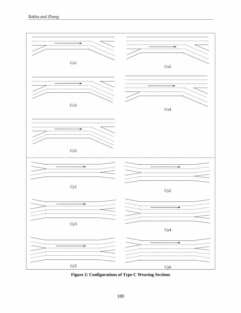
Rakha and Zhang

180

Cx1

Cx2

Cx3

Cx4

Cx5

Cy1

Cy2

Cy3

Cy4

Cy5

Cy6

Figure 2: Configurations of Type C Weaving Sections

Rakha and Zhang

181

0% 20% 40% 60% 80% 100%0.000.100.20

0.300.400.500.600.700.80

0.901.001.10

Volume Ratio

Capa

city

Fac

tor

SimulationHCM

Configuration Ax1, 150 m

0% 20% 40% 60% 80% 100%0.000.100.20

0.300.400.500.600.700.80

0.901.001.10

Volume Ratio

Cap

acity

Fac

tor

SimulationHCM

Configuration Ay1, 300 m

0% 20% 40% 60% 80% 100%0.000.100.20

0.300.400.500.600.700.80

0.901.001.10

Volume Ratio

Cap

acity

Fac

tor

SimulationHCM

Configuration Cx1, 450 m

0% 20% 40% 60% 80% 100%0.000.100.20

0.300.400.500.600.700.80

0.901.001.10

Volume Ratio

Capa

city

Fac

tor

SimulationHCM

Configuration Cy1, 600 m

Figure 3: Comparison of Simulation Results and Results from HCM Procedures

Rakha and Zhang

182

0% 20% 40% 60% 80% 100%

-0.20-0.100.000.100.200.300.400.500.600.700.800.901.001.10

Volume Ratio

Cap

acity

Fac

tor

Expo. PartSimulation(Simulation - Expo. Part)

Figure 4: Development of Exponential Model (Ax1, 750 m)

Rakha and Zhang

183

0.361

0.438

0.438

0.51

5

0.515

0.515

0.515

0.59

2

0.592

0.5920.592

0.6690.669

0.7460.823

0.9

VR

WR

0 0.2 0.4 0.6 0.8 10

0.1

0.2

0.3

0.4

0.5

0.6

0.7

0.8

0.9

1

Figure 5: Contour Plot of Capacity Factor for Weaving Section Cx1 (150 m)

Rakha and Zhang

184

Volume Percentage of FR

Volume Percentage of RF

Volume Percentage of RR

Weaving Section Length

F

Volume Percentage of FF

Figure 6: Structure of Artificial Neural Network 1

Rakha and Zhang

185

Volume Ratio

Weaving Ratio

Weaving Section Length

F

Figure 7: Structure of Artificial Neural Network 2

Rakha and Zhang

186

0% 20% 40% 60% 80% 100%0.000.100.20

0.300.400.500.600.700.80

0.901.001.10

Volume Ratio

Cap

acity

Fac

tor

TrendlineSimulation

Figure 8: Trend Line of Simulated Capacity of Configuration Cx2 (600 m)

Rakha and Zhang

187

0% 20% 40% 60% 80% 100%0.000.100.20

0.300.400.500.600.700.80

0.901.001.10

Volume Ratio

Capa

city

Fac

tor

SimulationExponential ModelHCM

0% 20% 40% 60% 80% 100%

0.000.100.20

0.300.400.500.600.700.80

0.901.001.10

Volume Ratio

Capa

city

Fac

tor

SimulationAngle ModelHCM

0% 20% 40% 60% 80% 100%0.000.100.20

0.300.400.500.600.700.80

0.901.001.10

Volume Ratio

Capa

city

Fac

tor

SimulationANN Model 1HCM

0% 20% 40% 60% 80% 100%

0.000.100.20

0.300.400.500.600.700.80

0.901.001.10

Volume Ratio

Capa

city

Fac

tor

SimulationANN Model 2HCM

0% 20% 40% 60% 80% 100%0.000.100.20

0.300.400.500.600.700.80

0.901.001.10

Volume Ratio

Capa

city

Fac

tor

SimulationSine ModelHCM

Figure 9: Modeling Simulated Capacity of Configuration Ax1 (750 m)

Rakha and Zhang

188

1 2 3 4 5 6 7 8 9 100.40

0.50

0.60

0.70

0.80

0.90

1.00

1.10

Days

Cap

acity

Fac

tor

Expo. ModelField

Exponential Model

Angle model does not apply.

1 2 3 4 5 6 7 8 9 100.40

0.50

0.60

0.70

0.80

0.90

1.00

1.10

Days

Cap

acity

Fac

tor

ANN Model 1Field

ANN Model 1

1 2 3 4 5 6 7 8 9 100.40

0.50

0.60

0.70

0.80

0.90

1.00

1.10

Days

Cap

acity

Fac

tor

ANN Model 2Field

ANN Model 2

1 2 3 4 5 6 7 8 9 100.40

0.50

0.60

0.70

0.80

0.90

1.00

1.10

Days

Cap

acity

Fac

tor

Sine ModelField

Sine Model

1 2 3 4 5 6 7 8 9 100.40

0.50

0.60

0.70

0.80

0.90

1.00

1.10

Days

Cap

acity

Fac

tor

HCMField

HCM

Figure 10: Model Validation with Field Data (Cx4)

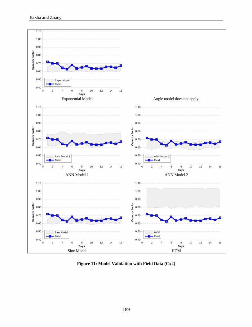
Rakha and Zhang

189

0 2 4 6 8 10 12 14 160.40

0.50

0.60

0.70

0.80

0.90

1.00

1.10

Days

Cap

acity

Fac

tor

Expo. ModelField

Exponential Model

Angle model does not apply.

0 2 4 6 8 10 12 14 160.40

0.50

0.60

0.70

0.80

0.90

1.00

1.10

Days

Cap

acity

Fac

tor

ANN Model 1Field

ANN Model 1

0 2 4 6 8 10 12 14 160.40

0.50

0.60

0.70

0.80

0.90

1.00

1.10

Days

Cap

acity

Fac

tor

ANN Model 2Field

ANN Model 2

0 2 4 6 8 10 12 14 160.40

0.50

0.60

0.70

0.80

0.90

1.00

1.10

Days

Cap

acity

Fac

tor

Sine ModelField

Sine Model

0 2 4 6 8 10 12 14 160.40

0.50

0.60

0.70

0.80

0.90

1.00

1.10

Days

Cap

acity

Fac

tor

HCMField

HCM

Figure 11: Model Validation with Field Data (Cx2)

Rakha and Zhang

190

Expo. Model Angle Model

ANN Model 1 ANN Model 2

Sine Model HCM

0.0

0.2

0.4

0.6

0.8

1.0

50 150 250 350 450 550 650 750

Weaving Section Length (m)

Cap

acity

Fac

tor

VR = 0.0 VR = 0.2VR = 0.4 VR = 0.6VR = 0.8 VR = 1.0

0.0

0.2

0.4

0.6

0.8

1.0

50 150 250 350 450 550 650 750Weaving Section Length (m)

Cap

acity

Fac

tor

VR = 0.0 VR = 0.2VR = 0.4 VR = 0.6VR = 0.8 VR = 1.0

0.0

0.2

0.4

0.6

0.8

1.0

50 150 250 350 450 550 650 750Weaving Section Length (m)

Cap

acity

Fac

tor

VR = 0.0 VR = 0.2VR = 0.4 VR = 0.6VR = 0.8 VR = 1.0

0.0

0.2

0.4

0.6

0.8

1.0

50 150 250 350 450 550 650 750Weaving Section Length (m)

Cap

acity

Fac

tor

VR = 0.0 VR = 0.2VR = 0.4 VR = 0.6VR = 0.8 VR = 1.0

0.0

0.2

0.4

0.6

0.8

1.0

50 150 250 350 450 550 650 750Weaving Section Length (m)

Cap

acity

Fac

tor

VR = 0.0 VR = 0.2VR = 0.4 VR = 0.6VR = 0.8 VR = 1.0

0.0

0.2

0.4

0.6

0.8

1.0

1.2

50 150 250 350 450 550 650 750Weaving Section Length (m)

Cap

acity

Fac

tor

VR = 0.0 VR = 0.2VR = 0.4 VR = 0.6VR = 0.8 VR = 1.0

Figure 12: Impact of Weaving Section Length on Capacity Factor (Cy3, WR = 0.5)

Rakha and Zhang

191

Expo. Model Angle Model

ANN Model 1 ANN Model 2

Sine Model HCM

0.0

0.2

0.4

0.6

0.8

1.0

0 0.2 0.4 0.6 0.8 1

VR

Cap

acity

Fac

tor

WR = 0.0 WR = 0.2WR = 0.4 WR = 0.6WR = 0.8 WR = 1.0

0.0

0.2

0.4

0.6

0.8

1.0

0 0.2 0.4 0.6 0.8 1VR

Cap

acity

Fac

tor

WR = 0.0 WR = 0.2WR = 0.4 WR = 0.6WR = 0.8 WR = 1.0

0.0

0.2

0.4

0.6

0.8

1.0

0 0.2 0.4 0.6 0.8 1VR

Cap

acity

Fac

tor

WR = 0.0 WR = 0.2WR = 0.4 WR = 0.6WR = 0.8 WR = 1.0

0.0

0.2

0.4

0.6

0.8

1.0

0 0.2 0.4 0.6 0.8 1VR

Cap

acity

Fac

tor

WR = 0.0 WR = 0.2WR = 0.4 WR = 0.6WR = 0.8 WR = 1.0

-0.8

-0.6

-0.4

-0.2

0.0

0.2

0.4

0.6

0.8

1.0

0 0.2 0.4 0.6 0.8 1

VR

Cap

acity

Fac

tor

WR = 0.0 WR = 0.2WR = 0.4 WR = 0.6WR = 0.8 WR = 1.0 0.0

0.2

0.4

0.6

0.8

1.0

1.2

0 0.2 0.4 0.6 0.8 1VR

Cap

acity

Fac

tor

WR = 0.0 WR = 0.2WR = 0.4 WR = 0.6WR = 0.8 WR = 1.0

Figure 13: Impact of Volume Ratio on Capacity Factor (Cy3, 300m)

Rakha and Zhang

192

0 0.2 0.4 0.6 0.8 10

0.2

0.4

0.6

0.8

1

Volume Ratio

Wea

ving

Rat

io

Ax1

0 0.2 0.4 0.6 0.8 10

0.2

0.4

0.6

0.8

1

Volume Ratio

Wea

ving

Rat

io

Ax2

0 0.2 0.4 0.6 0.8 10

0.2

0.4

0.6

0.8

1

Volume Ratio

Wea

ving

Rat

io

Ax3

0 0.2 0.4 0.6 0.8 10

0.2

0.4

0.6

0.8

1

Volume Ratio

Wea

ving

Rat

io

Ay1

0 0.2 0.4 0.6 0.8 10

0.2

0.4

0.6

0.8

1

Volume Ratio

Wea

ving

Rat

io

Ay2

0 0.2 0.4 0.6 0.8 10

0.2

0.4

0.6

0.8

1

Volume Ratio

Wea

ving

Rat

io

Cx1

0 0.2 0.4 0.6 0.8 10

0.2

0.4

0.6

0.8

1

Volume Ratio

Wea

ving

Rat

io

Cx2

0 0.2 0.4 0.6 0.8 10

0.2

0.4

0.6

0.8

1

Volume Ratio

Wea

ving

Rat

io

Cx3

0 0.2 0.4 0.6 0.8 10

0.2

0.4

0.6

0.8

1

Volume Ratio

Wea

ving

Rat

io

Cx4

0 0.2 0.4 0.6 0.8 10

0.2

0.4

0.6

0.8

1

Volume Ratio

Wea

ving

Rat

io

Cx5

0 0.2 0.4 0.6 0.8 10

0.2

0.4

0.6

0.8

1

Volume Ratio

Wea

ving

Rat

io

Cy1

0 0.2 0.4 0.6 0.8 10

0.2

0.4

0.6

0.8

1

Volume Ratio

Wea

ving

Rat

io

Cy2

0 0.2 0.4 0.6 0.8 10

0.2

0.4

0.6

0.8

1

Volume Ratio

Wea

ving

Rat

io

Cy3

0 0.2 0.4 0.6 0.8 10

0.2

0.4

0.6

0.8

1

Volume Ratio

Wea

ving

Rat

io

Cy4

0 0.2 0.4 0.6 0.8 10

0.2

0.4

0.6

0.8

1

Volume Ratio

Wea

ving

Rat

io

Cy5

0 0.2 0.4 0.6 0.8 10

0.2

0.4

0.6

0.8

1

Volume Ratio

Wea

ving

Rat

io

Cy6

Figure 14: Distribution of Simulated Data Points in VR-WR Plane

Rakha and Zhang

193

0 0.2 0.4 0.6 0.8 10

0.2

0.4

0.6

0.8

1

Volume Ratio

Wea

ving

Rat

io

demandthroughput

Figure 15: Comparing throughput and demand (Configuration Ax2, 450 m)

Rakha and Zhang

194

0 0.2 0.4 0.6 0.8 10

0.2

0.4

0.6

0.8

1

Volume Ratio

Wea

ving

Rat

io

Ax1

0 0.2 0.4 0.6 0.8 10

0.2

0.4

0.6

0.8

1

Volume RatioW

eavi

ng R

atio

Ax2

0 0.2 0.4 0.6 0.8 10

0.2

0.4

0.6

0.8

1

Volume Ratio

Wea

ving

Rat

io

Ax3

0 0.2 0.4 0.6 0.8 10

0.2

0.4

0.6

0.8

1

Volume Ratio

Wea

ving

Rat

io

Ay1

0 0.2 0.4 0.6 0.8 10

0.2

0.4

0.6

0.8

1

Volume Ratio

Wea

ving

Rat

io

Ay2

0 0.2 0.4 0.6 0.8 10

0.2

0.4

0.6

0.8

1

Volume Ratio

Wea

ving

Rat

io

Cx1

0 0.2 0.4 0.6 0.8 10

0.2

0.4

0.6

0.8

1

Volume RatioW

eavi

ng R

atio

Cx2

0 0.2 0.4 0.6 0.8 10

0.2

0.4

0.6

0.8

1

Volume Ratio

Wea

ving

Rat

io

Cx3

0 0.2 0.4 0.6 0.8 10

0.2

0.4

0.6

0.8

1

Volume Ratio

Wea

ving

Rat

io

Cx4

0 0.2 0.4 0.6 0.8 10

0.2

0.4

0.6

0.8

1

Volume Ratio

Wea

ving

Rat

io

Cx5

0 0.2 0.4 0.6 0.8 10

0.2

0.4

0.6

0.8

1

Volume Ratio

Wea

ving

Rat

io

Cy1

0 0.2 0.4 0.6 0.8 10

0.2

0.4

0.6

0.8

1

Volume RatioW

eavi

ng R

atio

Cy2

0 0.2 0.4 0.6 0.8 10

0.2

0.4

0.6

0.8

1

Volume Ratio

Wea

ving

Rat

io

Cy3

0 0.2 0.4 0.6 0.8 10

0.2

0.4

0.6

0.8

1

Volume Ratio

Wea

ving

Rat

io

Cy4

0 0.2 0.4 0.6 0.8 10

0.2

0.4

0.6

0.8

1

Volume Ratio

Wea

ving

Rat

io

Cy5

0 0.2 0.4 0.6 0.8 10

0.2

0.4

0.6

0.8

1

Volume Ratio

Wea

ving

Rat

io

Cy6

Figure 16: Distribution of Simulated Data Points in VR-WR Plane (Throughput)

Rakha and Zhang

195

Expo. Model Angle Model

ANN Model 1 ANN Model 2

Sine Model HCM

0.0

0.2

0.4

0.6

0.8

1.0

0 0.2 0.4 0.6 0.8 1

VR

Cap

acity

Fac

tor

WR = 0.0 WR = 0.2WR = 0.4 WR = 0.6WR = 0.8 WR = 1.0

0.0

0.2

0.4

0.6

0.8

1.0

0 0.2 0.4 0.6 0.8 1VR

Cap

acity

Fac

tor

WR = 0.0 WR = 0.2WR = 0.4 WR = 0.6WR = 0.8 WR = 1.0

0.0

0.2

0.4

0.6

0.8

1.0

0 0.2 0.4 0.6 0.8 1VR

Cap

acity

Fac

tor

WR = 0.0 WR = 0.2WR = 0.4 WR = 0.6WR = 0.8 WR = 1.0

0.0

0.2

0.4

0.6

0.8

1.0

0 0.2 0.4 0.6 0.8 1VR

Cap

acity

Fac

tor

WR = 0.0 WR = 0.2WR = 0.4 WR = 0.6WR = 0.8 WR = 1.0

0.0

0.2

0.4

0.6

0.8

1.0

0 0.2 0.4 0.6 0.8 1VR

Cap

acity

Fac

tor

WR = 0.0 WR = 0.2WR = 0.4 WR = 0.6WR = 0.8 WR = 1.0

0.0

0.2

0.4

0.6

0.8

1.0

1.2

0 0.2 0.4 0.6 0.8 1VR

Cap

acity

Fac

tor

WR = 0.0 WR = 0.2WR = 0.4 WR = 0.6WR = 0.8 WR = 1.0

Figure 17: Impact of Volume Ratio on Capacity Factor Excluding Points Far right to the Curves in Figure 14

Rakha and Zhang

196

APPENDIX 1: EXAMPLE PROBLEM

In the following the procedures for applying each of the three statistical models proposed in this paper are illustrated.

The Weaving Section A weaving section as shown below.

1100

50

100350

D

C A

B

The Question What is the capacity of this weaving section? The Facts Volume (A-C) = 1,100 veh/h Volume (A-D) = 100 veh/h Volume (B-C) = 50 veh/h Volume (B-D) = 350 veh/h 15 percent trucks PHF = 0.85 Rolling terrrian Drivers are regular commuters FFS = 100 km/h for freeway Capacity of 2,000 pc/h for on-ramp Weaving section length = 300 m

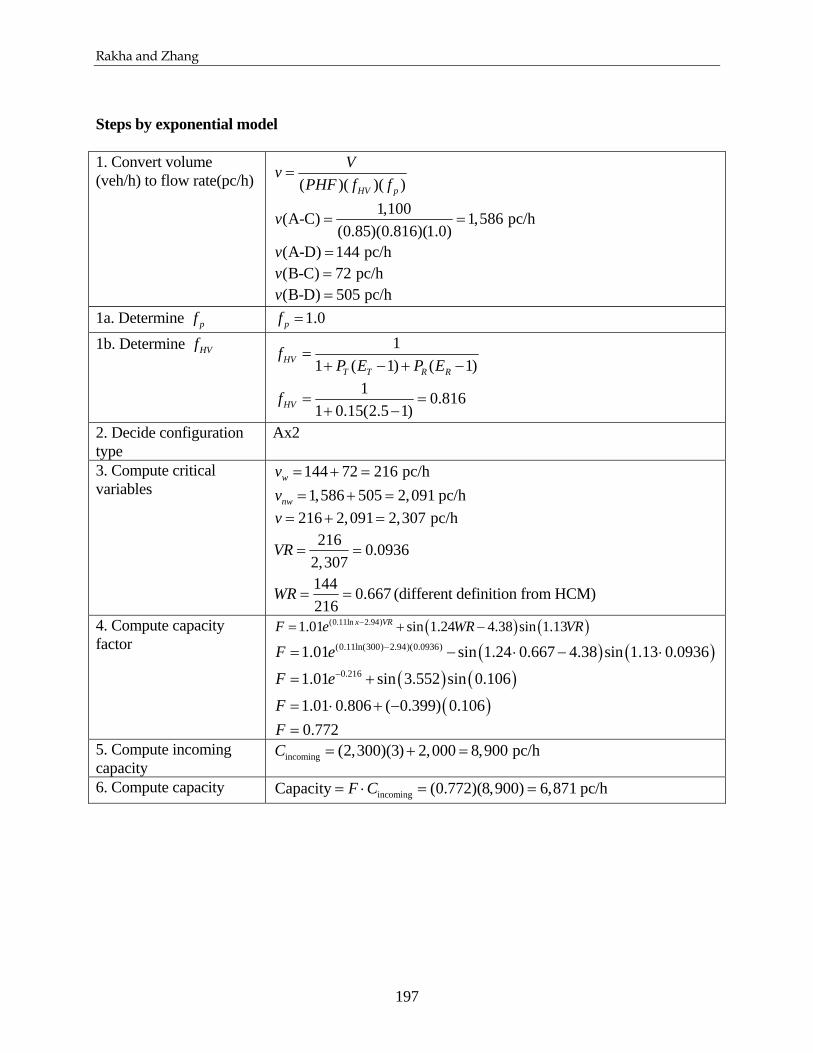
Rakha and Zhang

197

Steps by exponential model 1. Convert volume (veh/h) to flow rate(pc/h) ( )( )( )HV p

VvPHF f f

=

1,100(A-C) 1,586 pc/h(0.85)(0.816)(1.0)

v = =

(A-D) 144 pc/hv = (B-C) 72 pc/hv = (B-D) 505 pc/hv =

1a. Determine pf 1.0pf = 1b. Determine HVf 1

1 ( 1) ( 1)HVT T R R

fP E P E

=+ − + −

1 0.8161 0.15(2.5 1)HVf = =+ −

2. Decide configuration type

Ax2

3. Compute critical variables

144 72 216 pc/hwv = + = 1,586 505 2,091 pc/hnwv = + =

216 2,091 2,307 pc/hv = + = 216 0.0936

2,307VR = =

144 0.667216

WR = = (different definition from HCM)

4. Compute capacity factor

( ) ( )(0.11ln 2.94)1.01 sin 1.24 4.38 sin 1.13x VRF e WR VR−= + −

( ) ( )(0.11ln(300) 2.94)(0.0936)1.01 sin 1.24 0.667 4.38 sin 1.13 0.0936F e −= − ⋅ − ⋅

( ) ( )0.2161.01 sin 3.552 sin 0.106F e−= +

( )1.01 0.806 ( 0.399) 0.106F = ⋅ + − 0.772F =

5. Compute incoming capacity

incoming (2,300)(3) 2,000 8,900 pc/hC = + =

6. Compute capacity incomingCapacity (0.772)(8,900) 6,871 pc/hF C= ⋅ = =

Rakha and Zhang

198

Steps by angle model 1. Convert volume (veh/h) to flow rate(pc/h) ( )( )( )HV p

VvPHF f f

=

1,100(A-C) 1,586 pc/h(0.85)(0.816)(1.0)

v = =

(A-D) 144 pc/hv = (B-C) 72 pc/hv = (B-D) 505 pc/hv =

1a. Determine pf 1.0pf = 1b. Determine HVf 1

1 ( 1) ( 1)HVT T R R

fP E P E

=+ − + −

1 0.8161 0.15(2.5 1)HVf = =+ −

2. Decide configuration type

Ax2

3. Compute critical variables

144 72 216 pc/hwv = + = 1,586 505 2,091 pc/hnwv = + =

216 2,091 2,307 pc/hv = + = 216 0.0936

2,307VR = =

144 0.667216

WR = = (different definition from HCM)

4. Compute capacity factor 1 1

2 21 2

cos( ) ( )

VR b

VR b b WRθ −

⎛ ⎞⎟−⎜ ⎟⎜= ⎟⎜ ⎟⎜ ⎟⎟⎜ − + −⎝ ⎠

1 1

2 2

0.0936 0.08 0.174cos cos 1.452

1.473(0.0936 0.08) (2.13 0.667)θ − −

⎛ ⎞⎟+ ⎛ ⎞⎜ ⎟ ⎟⎜ ⎜= = =⎟ ⎟⎜ ⎜ ⎟⎟ ⎜⎜ ⎝ ⎠⎟⎟⎜ + + −⎝ ⎠

( ) 521 2 3 4( )aF a a a x aθ θ= + + +

( )2 0.0121.306 1.452 2.100 1.452 1.082 (300 49.7)F = ⋅ − ⋅ + − (0.786)(1.069) 0.840F = =

5. Compute incoming capacity

incoming (2,300)(3) 2,000 8,900 pc/hC = + =

6. Compute capacity incomingCapacity (0.840)(8,900) 7,480 pc/hF C= ⋅ = =

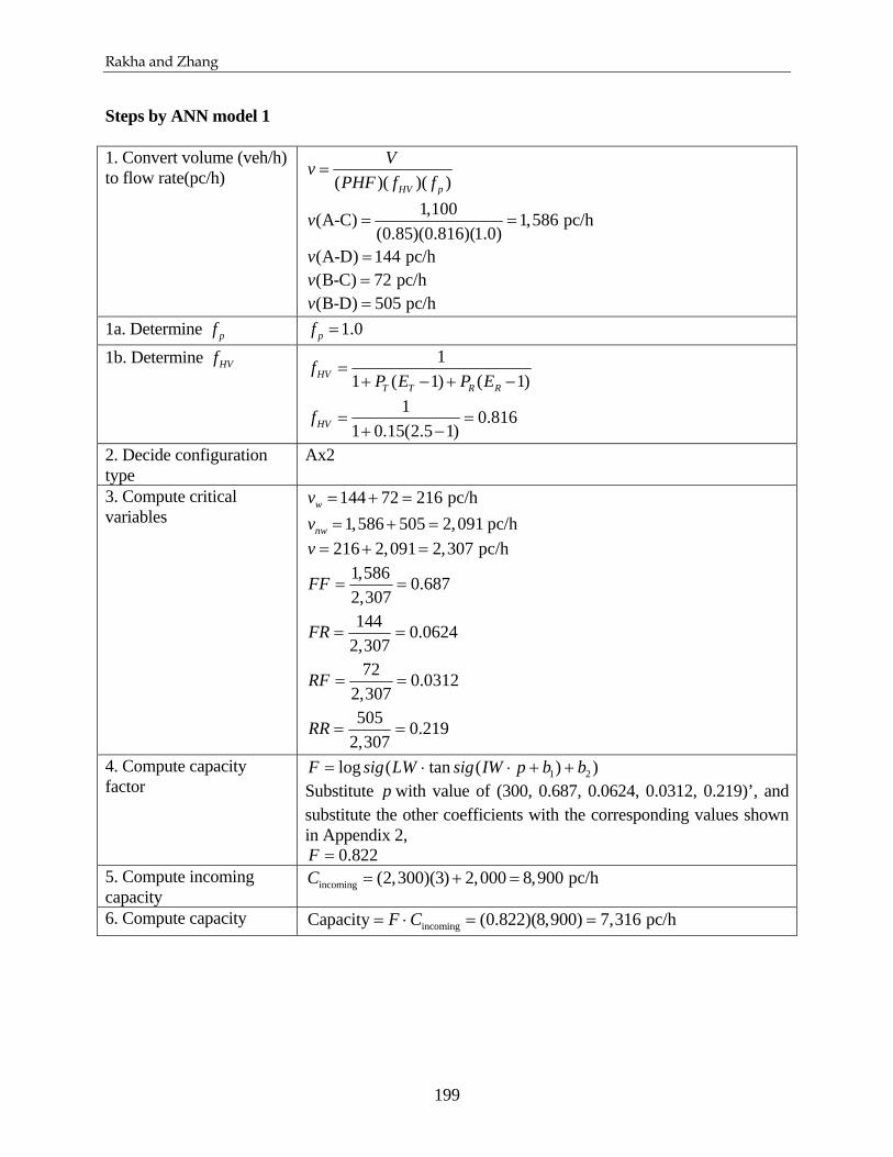
Rakha and Zhang

199

Steps by ANN model 1 1. Convert volume (veh/h) to flow rate(pc/h) ( )( )( )HV p

VvPHF f f

=

1,100(A-C) 1,586 pc/h(0.85)(0.816)(1.0)

v = =

(A-D) 144 pc/hv = (B-C) 72 pc/hv = (B-D) 505 pc/hv =

1a. Determine pf 1.0pf = 1b. Determine HVf 1

1 ( 1) ( 1)HVT T R R

fP E P E

=+ − + −

1 0.8161 0.15(2.5 1)HVf = =+ −

2. Decide configuration type

Ax2

3. Compute critical variables

144 72 216 pc/hwv = + = 1,586 505 2,091 pc/hnwv = + =

216 2,091 2,307 pc/hv = + = 1,586 0.6872,307

FF = =

144 0.06242,307

FR = =

72 0.03122,307

RF = =

505 0.2192,307

RR = =

4. Compute capacity factor

))(tan(log 21 bbpIWsigLWsigF ++⋅⋅= Substitute p with value of (300, 0.687, 0.0624, 0.0312, 0.219)’, and substitute the other coefficients with the corresponding values shown in Appendix 2,

0.822F = 5. Compute incoming capacity

incoming (2,300)(3) 2,000 8,900 pc/hC = + =

6. Compute capacity incomingCapacity (0.822)(8,900) 7,316 pc/hF C= ⋅ = =

Rakha and Zhang

200

Steps by ANN model 2 1. Convert volume (veh/h) to flow rate(pc/h) ( )( )( )HV p

VvPHF f f

=

1,100(A-C) 1,586 pc/h(0.85)(0.816)(1.0)

v = =

(A-D) 144 pc/hv = (B-C) 72 pc/hv = (B-D) 505 pc/hv =

1a. Determine pf 1.0pf = 1b. Determine HVf 1

1 ( 1) ( 1)HVT T R R

fP E P E

=+ − + −

1 0.8161 0.15(2.5 1)HVf = =+ −

2. Decide configuration type

Ax2

3. Compute critical variables

144 72 216 pc/hwv = + = 1,586 505 2,091 pc/hnwv = + =

216 2,091 2,307 pc/hv = + = 216 0.0936

2,307VR = =

144 0.667216

WR = = (different definition from HCM)

4. Compute capacity factor

))(tan(log 21 bbpIWsigLWsigF ++⋅⋅= Substitute p with value of (300, 0.0936, 0.667)’, and substitute the other coefficients with the corresponding values shown in Appendix 3,

0.835F = 5. Compute incoming capacity

incoming (2,300)(3) 2,000 8,900 pc/hC = + =

6. Compute capacity incomingCapacity (0.835)(8,900) 7,431 pc/hF C= ⋅ = =

Rakha and Zhang

201

Steps by sine model 1. Convert volume (veh/h) to flow rate(pc/h)

( )( )( )HV p

VvPHF f f

=

1,100(A-C) 1,586 pc/h(0.85)(0.816)(1.0)

v = =

(A-D) 144 pc/hv = (B-C) 72 pc/hv = (B-D) 505 pc/hv =

1a. Determine pf 1.0pf = 1b. Determine HVf 1

1 ( 1) ( 1)HVT T R R

fP E P E

=+ − + −

1 0.8161 0.15(2.5 1)HVf = =+ −

2. Decide configuration type

Ax2

3. Compute critical variables

144 72 216 pc/hwv = + = 1,586 505 2,091 pc/hnwv = + =

216 2,091 2,307 pc/hv = + = 216 0.0936

2,307VR = =

144 0.667216

WR = = (different definition from HCM)

4. Compute capacity factor

( )( )( ) ( ) ( )VRWRxVRF 36.0sin05.061.4sin5.2534.157.042.1sin93.0 021.0 ++−++−=

( )( )( )( ) ( )

0.0210.93sin 1.42 0.0936 0.57 1.34 300 25.5

sin 4.61 0.667 0.05 sin 0.36 0.0936

F = − ⋅ + + −

+ ⋅ + ⋅

( )( )( ) ( ) ( )0.0210.93sin 0.703 1.34 274.5 sin 3.12 sin 0.0337F = − + +

( )( ) ( )0.739 1.125 (0.0216) 0.0337 0.832F = + = 5. Compute incoming capacity

incoming (2,300)(3) 2,000 8,900 pc/hC = + =

6. Compute capacity

incomingCapacity (0.832)(8,900) 7,405 pc/hF C= ⋅ = =

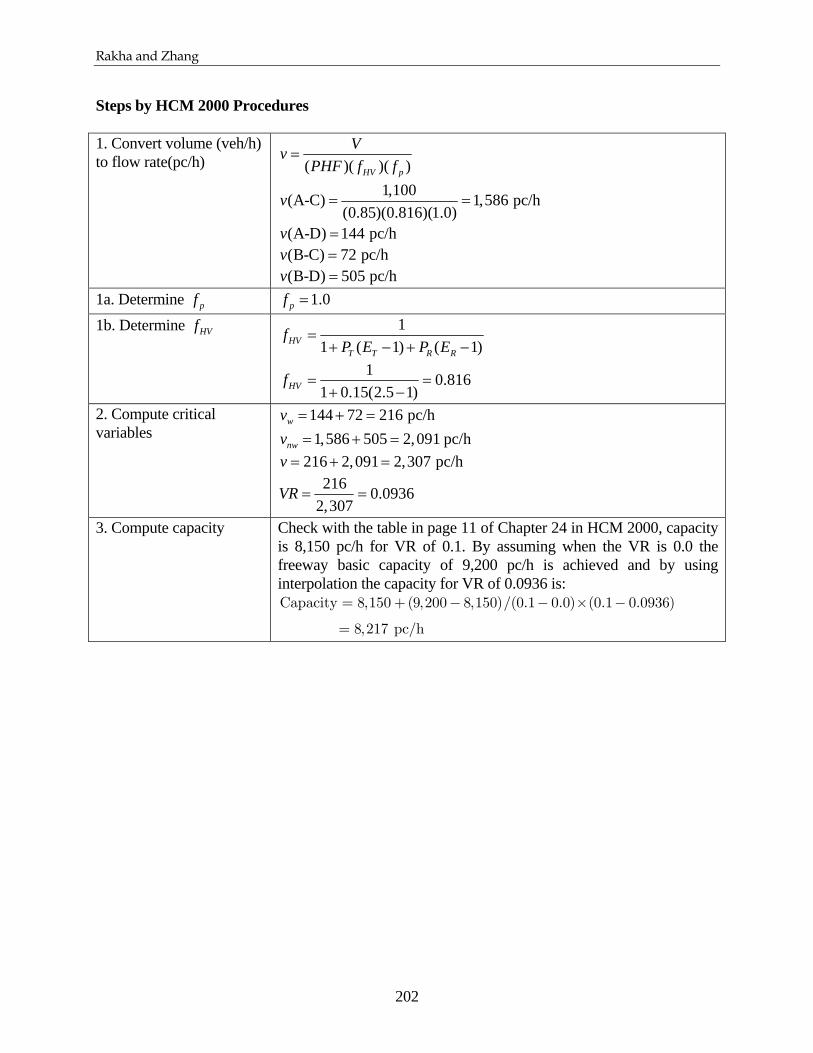
Rakha and Zhang

202

Steps by HCM 2000 Procedures 1. Convert volume (veh/h) to flow rate(pc/h) ( )( )( )HV p

VvPHF f f

=

1,100(A-C) 1,586 pc/h(0.85)(0.816)(1.0)

v = =

(A-D) 144 pc/hv = (B-C) 72 pc/hv = (B-D) 505 pc/hv =

1a. Determine pf 1.0pf = 1b. Determine HVf 1

1 ( 1) ( 1)HVT T R R

fP E P E

=+ − + −

1 0.8161 0.15(2.5 1)HVf = =+ −

2. Compute critical variables

144 72 216 pc/hwv = + = 1,586 505 2,091 pc/hnwv = + =

216 2,091 2,307 pc/hv = + = 216 0.0936

2,307VR = =

3. Compute capacity Check with the table in page 11 of Chapter 24 in HCM 2000, capacity is 8,150 pc/h for VR of 0.1. By assuming when the VR is 0.0 the freeway basic capacity of 9,200 pc/h is achieved and by using interpolation the capacity for VR of 0.0936 is: Capacity 8,150 (9,200 8,150)/(0.1 0.0) (0.1 0.0936)

8,217 pc/h

= + − − × −

=

Rakha and Zhang

203

APPENDIX 2: SAMPLE VALUES OF PARAMETERS IN ANN MODEL 1

))(tan(log 21 bbpIWsigLWsigF ++⋅⋅=

Where:

p : Column input vector (FF, FR, RF, RR, weaving section length)’

LW : Layer weight matrix

LW : Input weight matrix

1b , 2b : bias vectors

2

2tan ( ) 1

1 xsig x

e−= −

+

1

log ( )1 x

sig xe−

=+

Ax1

0.00128 -0.54672 -0.88876 -1.95210 -6.741000.00060 2.54730 -2.33300 -3.60570 -13.020000.00050 6.08910 -8.59220 -9.44690 15.45200-0.00065 1.48150 2.06930 -0.90995 3.01920-0.00028 -2.15800 1.77940 14.13000 13.730000.02

IW =

411 -2.00520 0.56913 -21.95500 7.96440

⎡ ⎤⎢ ⎥⎢ ⎥⎢ ⎥⎢ ⎥⎢ ⎥⎢ ⎥⎢ ⎥⎣ ⎦

1

0.56821-0.98434-8.28600-1.08340-1.195600.66455

b

⎡ ⎤⎢ ⎥⎢ ⎥⎢ ⎥

= ⎢ ⎥⎢ ⎥⎢ ⎥⎢ ⎥⎣ ⎦

[ ]-2.32110 -1.65370 5.78510 -4.51930 -1.40370 0.28584LW =

2 6.03540b =

Rakha and Zhang

204

Ax2

-0.58238 8.61420 -15.74300 0.86334 10.23600-0.02017 14.31600 -28.05600 19.36800 -4.74380-0.06678 -11.31000 -6.67480 -4.43210 -0.288600.30336 -2.58950 5.73110 1.80330 6.70370-0.00017 -2.73060 0.09603 -0.78396 1.126300

IW =

.00024 2.89380 -2.27660 -3.53160 -9.89390

⎡ ⎤⎢ ⎥⎢ ⎥⎢ ⎥⎢ ⎥⎢ ⎥⎢ ⎥⎢ ⎥⎣ ⎦

1

-12.20900-23.71500-16.567008.028002.52710-1.23820

b

⎡ ⎤⎢ ⎥⎢ ⎥⎢ ⎥

= ⎢ ⎥⎢ ⎥⎢ ⎥⎢ ⎥⎣ ⎦

[ ]-25.63800 21.03700 -0.45223 14.97200 -9.26320 -4.28330LW =

2 -16.15000b =

Ax3

-1.61350 1.47040 -2.39430 -12.76600 -7.558700.00014 1.54260 3.09920 -14.15100 -2.99990-0.00019 0.66739 -0.32395 6.32800 -7.708200.01654 -2.02930 4.57170 -8.49730 14.20800-0.95972 0.33898 4.13650 -10.67500 4.391900.000

IW =

37 6.13900 0.03371 3.48170 0.58682

⎡ ⎤⎢ ⎥⎢ ⎥⎢ ⎥⎢ ⎥⎢ ⎥⎢ ⎥⎢ ⎥⎣ ⎦

1

-0.96583-1.080300.616420.36997-0.24483-4.62160

b

⎡ ⎤⎢ ⎥⎢ ⎥⎢ ⎥

= ⎢ ⎥⎢ ⎥⎢ ⎥⎢ ⎥⎣ ⎦

[ ]0.06341 -2.40620 -1.78060 0.40935 0.06869 1.44940LW =

2 0.08691b =

Rakha and Zhang

205

Ay1

-0.00009 -0.40010 -2.82170 6.96960 -7.297500.24897 2.59990 0.55521 11.31600 -4.24970-0.00061 -3.49750 8.20180 -2.75530 3.226700.02643 1.14150 -0.28437 -3.26500 2.271800.00010 2.28890 -1.08990 8.07280 10.16200-0.00019

IW =

1.78610 -0.46390 18.56700 1.87850

⎡ ⎤⎢ ⎥⎢ ⎥⎢ ⎥⎢ ⎥⎢ ⎥⎢ ⎥⎢ ⎥⎣ ⎦

1

1.86290-4.837302.64050-3.11900-4.40210-1.85850

b

⎡ ⎤⎢ ⎥⎢ ⎥⎢ ⎥

= ⎢ ⎥⎢ ⎥⎢ ⎥⎢ ⎥⎣ ⎦

[ ]3.58330 2.51520 0.69912 0.16819 5.05430 -3.54670LW =

2 1.66460b =

Ay2

0.00218 1.29500 1.33380 -33.83300 9.274900.00013 2.84970 -2.79770 5.40940 14.748000.00111 -0.09983 -1.43050 12.42400 7.775000.00012 1.68720 -5.17480 -2.36100 7.36320-0.00115 0.89579 2.38910 -10.13700 -5.966600.02518 0

IW =

.34844 -0.86557 -1.77720 15.34500

⎡ ⎤⎢ ⎥⎢ ⎥⎢ ⎥⎢ ⎥⎢ ⎥⎢ ⎥⎢ ⎥⎣ ⎦

1

-3.08400-5.68020-1.73770-2.797100.62629-3.73900

b

⎡ ⎤⎢ ⎥⎢ ⎥⎢ ⎥

= ⎢ ⎥⎢ ⎥⎢ ⎥⎢ ⎥⎣ ⎦

[ ]-0.27324 44.45700 -9.51510 -14.53400 -9.66420 0.16763LW =

2 29.39300b =

Rakha and Zhang

206

Cx1

-0.02865 6.50410 -7.34640 -7.31220 -5.83520-0.01249 -5.38260 -0.17863 2.70030 16.28600-0.00001 3.27430 2.55610 -6.41460 -11.63700-0.00022 2.78930 -0.02999 -6.85590 -10.540000.00019 -2.88830 3.46540 -7.07300 -2.967800.

IW =

39761 -3.47490 -1.08660 -5.30650 14.05400

⎡ ⎤⎢ ⎥⎢ ⎥⎢ ⎥⎢ ⎥⎢ ⎥⎢ ⎥⎢ ⎥⎣ ⎦

1

4.091900.609491.033203.199500.215500.01477

b

⎡ ⎤⎢ ⎥⎢ ⎥⎢ ⎥

= ⎢ ⎥⎢ ⎥⎢ ⎥⎢ ⎥⎣ ⎦

[ ]0.04063 -0.44693 -22.62600 5.95870 0.49914 7.62500LW =

2 8.16280b =

Cx2

-0.00033 -1.97140 1.98090 -8.61810 -0.78407-0.27020 -3.81630 -1.35200 -9.00940 5.524300.26374 -3.30310 -3.53380 1.85170 -11.707000.01363 -0.33655 -0.37058 -10.74000 -11.40100-0.00029 -3.10230 -0.27114 -2.29680 -5.9642

IW =

00.00030 -2.28530 -3.02510 4.21960 -4.86370

⎡ ⎤⎢ ⎥⎢ ⎥⎢ ⎥⎢ ⎥⎢ ⎥⎢ ⎥⎢ ⎥⎣ ⎦

1

2.483404.938701.123402.023001.540604.04300

b

⎡ ⎤⎢ ⎥⎢ ⎥⎢ ⎥

= ⎢ ⎥⎢ ⎥⎢ ⎥⎢ ⎥⎣ ⎦

[ ]0.69180 0.41943 0.33209 1.03110 -0.68884 -2.49940LW =

2 1.35480b =

Rakha and Zhang

207

Cx3

0.02376 5.85390 -4.28190 28.29500 -1.45860-0.00015 3.75850 1.87540 27.54700 -25.38000-0.00085 -1.77670 0.47798 7.85230 14.918000.00041 2.14360 1.54870 6.20410 14.93400-0.00052 5.90770 -4.01730 13.19700 -11.646001.4899

IW =

0 -2.57360 -0.64497 4.80880 -8.97610

⎡ ⎤⎢ ⎥⎢ ⎥⎢ ⎥⎢ ⎥⎢ ⎥⎢ ⎥⎢ ⎥⎣ ⎦

1

-2.135103.77490-1.17870-4.011201.313000.29993

b

⎡ ⎤⎢ ⎥⎢ ⎥⎢ ⎥

= ⎢ ⎥⎢ ⎥⎢ ⎥⎢ ⎥⎣ ⎦

[ ]0.25282 -14.03400 0.63783 1.35340 -0.34031 6.90290LW =

2 7.55120b =

Cx4

-0.00012 1.45540 3.00960 -7.40920 -6.705800.02183 -2.93440 0.26529 1.23550 1.406700.02809 5.05730 -6.87640 -7.70370 -16.96400-0.00004 -1.98210 -1.44710 -2.66150 -2.109100.24768 1.40200 2.76520 10.28700 -7.41160-0.021

IW =

45 2.85750 0.82511 -11.20900 -11.56300

⎡ ⎤⎢ ⎥⎢ ⎥⎢ ⎥⎢ ⎥⎢ ⎥⎢ ⎥⎢ ⎥⎣ ⎦

1

-0.900900.97840-0.822791.58400-1.344200.80795

b

⎡ ⎤⎢ ⎥⎢ ⎥⎢ ⎥

= ⎢ ⎥⎢ ⎥⎢ ⎥⎢ ⎥⎣ ⎦

[ ]-7.13440 -2.59420 0.08576 16.65900 1.09380 -2.83320LW =

2 1.55750b =

Rakha and Zhang

208

Cx5

-0.00179 -0.85505 -4.06900 10.07800 10.865000.00010 1.98380 1.56930 10.74400 -5.21570-0.00119 -1.82520 2.24560 -5.14650 -3.192100.00685 -2.88180 -1.87650 12.02600 4.20260-0.00006 -1.17320 -2.74260 3.83800 6.06240-0.01

IW =

878 1.16960 1.85470 14.64200 7.71800

⎡ ⎤⎢ ⎥⎢ ⎥⎢ ⎥⎢ ⎥⎢ ⎥⎢ ⎥⎢ ⎥⎣ ⎦

1

0.413590.768712.175900.626860.31781-3.15710

b

⎡ ⎤⎢ ⎥⎢ ⎥⎢ ⎥

= ⎢ ⎥⎢ ⎥⎢ ⎥⎢ ⎥⎣ ⎦

[ ]-0.94349 -8.49320 1.17800 0.59599 3.49960 -0.46605LW =

2 8.18520b =

Cy1

0.00031 -1.16600 -5.26440 -4.11700 3.193100.00035 -7.76380 -9.31460 -6.61510 5.172700.06263 -10.78800 -2.73530 -5.00150 1.339300.00010 4.62410 0.98252 -3.23590 -1.171800.00241 0.10650 -8.98610 2.55730 -2.647500.00132 -

IW =

3.91370 7.94100 -7.30020 6.30220

⎡ ⎤⎢ ⎥⎢ ⎥⎢ ⎥⎢ ⎥⎢ ⎥⎢ ⎥⎢ ⎥⎣ ⎦

1

-0.955012.513600.058670.12130-0.83389-1.15280

b

⎡ ⎤⎢ ⎥⎢ ⎥⎢ ⎥

= ⎢ ⎥⎢ ⎥⎢ ⎥⎢ ⎥⎣ ⎦

[ ]-0.84325 -0.52567 0.10492 2.12610 0.08051 -0.08641LW =

2 0.36715b =

Rakha and Zhang

209

Cy2

0.00910 -2.03320 4.16470 -5.16680 -9.93410-0.00714 -1.91980 5.37660 6.46950 0.127990.18684 -0.82203 3.28870 -4.57880 21.407000.00247 -1.17080 3.64260 -32.67500 18.675000.00018 1.80360 -0.01022 -13.34100 -12.719000.423

IW =

51 -2.85580 -3.64760 -11.39300 2.71870

⎡ ⎤⎢ ⎥⎢ ⎥⎢ ⎥⎢ ⎥⎢ ⎥⎢ ⎥⎢ ⎥⎣ ⎦

1

-2.452900.53500-3.02940-0.701670.50397-0.00184

b

⎡ ⎤⎢ ⎥⎢ ⎥⎢ ⎥

= ⎢ ⎥⎢ ⎥⎢ ⎥⎢ ⎥⎣ ⎦

[ ]-0.05545 -0.10991 0.07014 -0.29513 2.40560 4.22470LW =

2 -2.79160b =

Cy3

0.01170 5.26910 -12.95100 4.95020 8.49980-0.00077 -5.30820 2.72050 0.56758 0.638670.00027 4.58320 4.49230 -3.44020 0.629260.00136 0.99409 1.53880 0.45573 0.797600.00043 8.12970 7.38510 -0.10348 3.006501.18020 3.89110 -4

IW =

.09400 -0.54326 1.37970

⎡ ⎤⎢ ⎥⎢ ⎥⎢ ⎥⎢ ⎥⎢ ⎥⎢ ⎥⎢ ⎥⎣ ⎦

1

13.515000.77802-1.18490-3.91970-3.74520-1.35010

b

⎡ ⎤⎢ ⎥⎢ ⎥⎢ ⎥

= ⎢ ⎥⎢ ⎥⎢ ⎥⎢ ⎥⎣ ⎦

[ ]-10.83400 -0.45462 -4.20200 -16.35400 4.78710 -5.20710LW =

2 0.14868b =

Rakha and Zhang

210

Cy4

0.00005 -6.32000 5.72410 2.87220 -2.82560-0.00003 5.15310 -6.56870 2.03880 6.15420-0.00085 2.87100 1.90200 7.84780 4.135800.00079 -0.73342 -4.92190 -6.88340 -5.067200.04647 -2.16310 3.07200 -5.80830 -6.10290-0.00126 3.

IW =

41900 -1.95260 4.86430 -8.54340

⎡ ⎤⎢ ⎥⎢ ⎥⎢ ⎥⎢ ⎥⎢ ⎥⎢ ⎥⎢ ⎥⎣ ⎦

1

4.44390-5.16890-3.390503.465700.24827-0.51983

b

⎡ ⎤⎢ ⎥⎢ ⎥⎢ ⎥

= ⎢ ⎥⎢ ⎥⎢ ⎥⎢ ⎥⎣ ⎦

[ ]4.12910 5.08400 0.53879 1.04930 0.18809 0.21382LW =

2 0.64677b =

Cy5

0.02143 1.47470 -6.46930 3.53070 -3.674800.00005 5.72400 4.97480 2.67970 -4.29660-0.00016 2.85420 3.19250 1.20690 -3.299600.00090 4.47820 -3.53890 0.53269 -3.45440-0.01773 3.44480 -3.89060 2.86840 3.79670-0.00019 7.333

IW =

10 4.13560 -2.45020 -1.83240

⎡ ⎤⎢ ⎥⎢ ⎥⎢ ⎥⎢ ⎥⎢ ⎥⎢ ⎥⎢ ⎥⎣ ⎦

1

1.16380-0.288100.17362-0.42314-0.87601-2.17280

b

⎡ ⎤⎢ ⎥⎢ ⎥⎢ ⎥

= ⎢ ⎥⎢ ⎥⎢ ⎥⎢ ⎥⎣ ⎦

[ ]0.01348 1.59950 -1.90630 0.18450 -0.25180 2.72370LW =

2 2.06970b =

Rakha and Zhang

211

Cy6

0.20353 -14.03300 -12.88500 -0.51044 -2.988600.01153 -14.62900 14.65800 -0.74916 -2.846100.00026 -11.98000 -15.62000 -2.55690 -2.13020-0.00004 0.79918 1.52400 -5.49060 -2.524700.22445 12.99300 1.56980 0.30638 -1.5767

IW =

00.00071 -1.09550 -1.31910 -0.14278 3.81840

⎡ ⎤⎢ ⎥⎢ ⎥⎢ ⎥⎢ ⎥⎢ ⎥⎢ ⎥⎢ ⎥⎣ ⎦

1

1.08610-4.227502.284800.78479-1.82930-2.14700

b

⎡ ⎤⎢ ⎥⎢ ⎥⎢ ⎥

= ⎢ ⎥⎢ ⎥⎢ ⎥⎢ ⎥⎣ ⎦

[ ]-0.19541 -0.13045 8.52540 -8.62030 -0.23548 1.52450LW =

2 0.97845b =

Rakha and Zhang

212

APPENDIX 3: SAMPLE VALUES OF PARAMETERS IN ANN MODEL 2

))(tan(log 21 bbpIWsigLWsigF ++⋅⋅=

Where:

p : Column input vector (FF, FR, RF, RR, weaving section length)’

LW : Layer weight matrix

LW : Input weight matrix

1b , 2b : bias vectors

2

2tan ( ) 1

1 xsig x

e−= −

+

1

log ( )1 x

sig xe−

=+

Ax1

0.00043 -0.74048 4.08970-0.00621 0.92472 -0.838050.00030 10.51100 0.22824-0.00012 1.16000 -0.49750

IW

⎡ ⎤⎢ ⎥⎢ ⎥=⎢ ⎥⎢ ⎥⎣ ⎦

1

-3.04650-1.426600.377720.97783

b

⎡ ⎤⎢ ⎥⎢ ⎥=⎢ ⎥⎢ ⎥⎣ ⎦

[ ]-1.23420 -5.64570 -5.65690 -7.36700LW =

2 6.04610b =

Rakha and Zhang

213

Ax2

-0.00023 2.28470 0.03187-0.00013 1.67040 0.242390.26559 1.46900 4.81860-0.10088 0.99141 4.72490

IW

⎡ ⎤⎢ ⎥⎢ ⎥=⎢ ⎥⎢ ⎥⎣ ⎦

1

-1.67590-1.43370-4.2617010.67800

b

⎡ ⎤⎢ ⎥⎢ ⎥=⎢ ⎥⎢ ⎥⎣ ⎦

[ ]10.88000 -15.05800 -2.24440 -0.10961LW =

2 1.28190b =

Ax3

-0.00044 3.99670 -0.552620.15989 -2.76360 3.379000.00004 0.42477 2.388100.00037 3.81410 -1.79760

IW

⎡ ⎤⎢ ⎥⎢ ⎥=⎢ ⎥⎢ ⎥⎣ ⎦

1

0.28644-1.58800-2.11410-1.24430

b

⎡ ⎤⎢ ⎥⎢ ⎥=⎢ ⎥⎢ ⎥⎣ ⎦

[ ]-2.16730 0.64276 -1.54320 -0.04004LW =

2 0.90154b =

Ay1

-0.00012 5.91280 0.098880.00029 -0.25589 -1.62820-0.00029 0.68899 1.442300.03434 -2.75290 4.03170

IW

⎡ ⎤⎢ ⎥⎢ ⎥=⎢ ⎥⎢ ⎥⎣ ⎦

1

0.580890.46467-0.83592-4.42330

b

⎡ ⎤⎢ ⎥⎢ ⎥=⎢ ⎥⎢ ⎥⎣ ⎦

[ ]-6.79330 -4.30650 -4.43460 0.17287LW =

2 6.08270b =

Rakha and Zhang

214

Ay2

0.00058 -1.71370 -2.23250-0.00055 0.35075 -3.234900.00012 -4.79250 -0.00981-0.08956 -8.30360 -8.07500

IW

⎡ ⎤⎢ ⎥⎢ ⎥=⎢ ⎥⎢ ⎥⎣ ⎦

1

2.049401.47820-1.28890-3.78240

b

⎡ ⎤⎢ ⎥⎢ ⎥=⎢ ⎥⎢ ⎥⎣ ⎦

[ ]1.17680 -0.69738 19.89800 -11.14000LW =

2 8.59160b =

Cx1

0.00005 -3.66780 -0.866220.34731 0.42565 -1.919900.00001 -3.11560 0.41704-0.00147 -3.92080 -5.54830

IW

⎡ ⎤⎢ ⎥⎢ ⎥=⎢ ⎥⎢ ⎥⎣ ⎦

1

2.58570-2.347001.516007.96040

b

⎡ ⎤⎢ ⎥⎢ ⎥=⎢ ⎥⎢ ⎥⎣ ⎦

[ ]-3.11880 0.06048 3.75440 -0.75018LW =

2 0.54093b =

Cx2

0.00006 -2.31590 3.004700.31903 -0.11980 -1.76280-0.01315 -0.23963 0.35937-0.00039 -6.41840 -6.01960

IW

⎡ ⎤⎢ ⎥⎢ ⎥=⎢ ⎥⎢ ⎥⎣ ⎦

1

-0.823183.42760-0.996410.31761

b

⎡ ⎤⎢ ⎥⎢ ⎥=⎢ ⎥⎢ ⎥⎣ ⎦

[ ]0.87753 -2.24960 -5.74270 0.88766LW =

2 -1.97910b =

Rakha and Zhang

215

Cx3

0.00324 -2.95020 -9.865700.00014 -1.52310 -2.50060-0.00005 1.73190 -0.34100-0.35207 -3.13260 0.83528

IW

⎡ ⎤⎢ ⎥⎢ ⎥=⎢ ⎥⎢ ⎥⎣ ⎦

1

8.387003.42140-0.697412.11180

b

⎡ ⎤⎢ ⎥⎢ ⎥=⎢ ⎥⎢ ⎥⎣ ⎦

[ ]0.69896 -6.12270 -2.13020 -2.15350LW =

2 2.28470b =

Cx4

0.32949 0.80537 2.645600.01303 2.01730 0.470440.01367 1.76040 0.45371-0.00027 2.85300 -1.70080

IW

⎡ ⎤⎢ ⎥⎢ ⎥=⎢ ⎥⎢ ⎥⎣ ⎦

1

9.18840-0.95607-1.00520-0.44296

b

⎡ ⎤⎢ ⎥⎢ ⎥=⎢ ⎥⎢ ⎥⎣ ⎦

[ ]-10.01700 -12.91700 12.50300 -0.96826LW =

2 10.81400b =

Cx5

-0.00112 -3.51250 -0.30972-0.00041 2.81680 -1.02900-0.00106 -3.80430 -0.781810.01273 -0.31123 -1.18190

IW

⎡ ⎤⎢ ⎥⎢ ⎥=⎢ ⎥⎢ ⎥⎣ ⎦

1

2.34330-0.189882.66730-0.29849

b

⎡ ⎤⎢ ⎥⎢ ⎥=⎢ ⎥⎢ ⎥⎣ ⎦

[ ]2.90630 -1.31340 -3.08440 0.37988LW =

2 0.51538b =

Rakha and Zhang

216

Cy1

-0.00171 -3.70740 -0.268230.00014 -5.98210 4.092600.00087 -3.19550 -0.62817-0.00013 4.00390 1.64400

IW

⎡ ⎤⎢ ⎥⎢ ⎥=⎢ ⎥⎢ ⎥⎣ ⎦

1

-1.881501.547602.57620-2.38000

b

⎡ ⎤⎢ ⎥⎢ ⎥=⎢ ⎥⎢ ⎥⎣ ⎦

[ ]0.02379 -0.77707 0.27354 -0.90942LW =

2 0.05398b =

Cy2

-0.00003 3.99350 4.59770-0.00016 1.87330 0.43174-0.00027 3.01820 -3.30350-0.51240 -1.99990 2.92480

IW

⎡ ⎤⎢ ⎥⎢ ⎥=⎢ ⎥⎢ ⎥⎣ ⎦

1

0.66301-0.85240-0.08324-0.02551

b

⎡ ⎤⎢ ⎥⎢ ⎥=⎢ ⎥⎢ ⎥⎣ ⎦

[ ]2.18310 -2.09380 0.85074 0.49385LW =

2 -1.23630b =

Cy3

-0.00054 3.56880 1.412100.08359 25.56000 6.529400.66754 -2.73240 -0.49917-0.00161 -6.38040 -6.83180

IW

⎡ ⎤⎢ ⎥⎢ ⎥=⎢ ⎥⎢ ⎥⎣ ⎦

1

-1.77470-18.188000.213488.10690

b

⎡ ⎤⎢ ⎥⎢ ⎥=⎢ ⎥⎢ ⎥⎣ ⎦

[ ]-0.91903 0.08123 0.54977 0.21354LW =

2 -0.33933b =

Rakha and Zhang

217

Cy4

-0.00592 2.05590 -1.603500.00062 -2.09590 -0.55043-0.00636 1.31320 0.916780.00045 -3.37610 3.10640

IW

⎡ ⎤⎢ ⎥⎢ ⎥=⎢ ⎥⎢ ⎥⎣ ⎦

1

3.786600.974690.512020.28018

b

⎡ ⎤⎢ ⎥⎢ ⎥=⎢ ⎥⎢ ⎥⎣ ⎦

[ ]0.13590 2.17370 0.13915 -0.79883LW =

2 0.17869b =

Cy5

0.02732 2.81580 1.45090-0.00011 2.20970 1.073400.00000 -5.07790 -1.144200.50117 -0.63018 -1.40100

IW

⎡ ⎤⎢ ⎥⎢ ⎥=⎢ ⎥⎢ ⎥⎣ ⎦

1

-4.07840-1.187901.906801.76650

b

⎡ ⎤⎢ ⎥⎢ ⎥=⎢ ⎥⎢ ⎥⎣ ⎦

[ ]0.20779 -1.29210 0.14312 0.41053LW =

2 0.03166b =

Cy6

0.13075 1.80160 2.08240-0.00029 3.39620 1.185900.01456 5.46330 3.979900.19331 0.95737 2.89720

IW

⎡ ⎤⎢ ⎥⎢ ⎥=⎢ ⎥⎢ ⎥⎣ ⎦

1

2.51780-1.45830-4.00330-1.52900

b

⎡ ⎤⎢ ⎥⎢ ⎥=⎢ ⎥⎢ ⎥⎣ ⎦

[ ]-0.16075 -1.36500 0.32853 -0.23385LW =

2 0.71097b =

218

Chapter 8. Summary, Conclusions, and Future Work

8.1 Summary and conclusions In this study one of the most important aspects of analysis of freeway weaving sections was examined, namely estimating the capacity of freeway weaving sections.

The very first task of this study was to validate the INTEGRATION microscopic traffic simulation software for the modeling of freeway weaving sections. This validation effort was required in order to utilize the software for developing the weaving capacity analytical procedures. The validation effort compared the spatial distribution of lane changes along weaving sections to field data collected on nine different freeway weaving sections in Los Angeles, CA. The lane-changing logic within the INTEGRATION software was presented and validated against field data collected on five Type-C freeway weaving sections. In this study, the vehicle demand distribution, both total and by movement, across the weaving lanes were compared in order to validate the lateral and longitudinal lane-changing activity logic. The analysis demonstrated that the lane-changing behavior within a weaving section is an extremely complicated phenomenon that is affected by many factors, including the geometric configuration of the weaving section and the O-D demand. The study also demonstrated that even at the same weaving site, lane-changing behavior of vehicles varies considerably, depending on the traffic conditions and O-D demand. The results demonstrate significant agreement between the simulation results and the field data for most type-C weaving sections. In the cases for which the results did not agree, it appeared that the vehicle distribution prior to entering the weave section was critical. The study demonstrated how the use of optional lane-bias and lane-changing parameters can enhance the consistency between the INTEGRATION results and the field data. In conclusion, it appears that the INTEGRATION model offers a robust tool for the modeling and evaluation of weaving sections.

A validation of the INTEGRATION software capacity estimates was conducted using data from the Queen Elizabeth Way (QEW) in Toronto. The findings and conclusions of the study can be summarized as follows:

a. The study demonstrated the validity of the INTEGRATION software for the analysis of weaving section capacities.

b. The study demonstrated some questionable capacity estimates by the CORSIM software and a gap acceptance procedure proposed in the literature. Specifically, the results demonstrated an unrealistic increase in roadway capacity with an increase in the mainline weaving volume for a Type B weaving section.

c. The study demonstrated that the random number seed resulted in a weaving section capacity standard deviation of 65 veh/h/lane.

d. The weaving ratio, which is the ratio of the lowest weaving volume to the total weaving volume, has a significant impact on the capacity of weaving sections. Specifically, differences in the range 326 veh/h/lane were observed in this study. Unfortunately, the weaving ratio is not considered in the HCM 2000 procedures.

e. The length of a weaving section has a larger impact on the capacity of weaving sections as the length of the weaving section decreases and the traffic demand increases.

219

f. There does not exist enough evidence to conclude that the speed differential between freeway and ramp traffic has a significant impact on weaving section capacities.

g. The HCM procedures for accounting for heavy duty vehicle impacts on weaving section capacities appear to be reasonable.

h. Weaving sections requiring no lane changing by weaving vehicles should not be considered Type B weaving sections.

i. Simulation is a very useful tool for the capacity analysis of freeway weaving sections. Having demonstrated the validity of the INTEGATION software for the modeling of weaving sections, the INTEGRATION software was utilized to construct a database of weaving section capacities. This database was then used to develop analytical procedures for estimating the capacity of weaving sections. The simulation results demonstrate that the HCM procedures are not only inadequate but fail to capture critical variables that impact the capacity of weaving sections, including the weaving ratio and the distribution of the weaving volume between freeway-to-ramp and ramp-to-freeway. The HCM procedures tend to over estimate the capacity of Type B weaving sections for this study and an earlier study presented by Lertworawanich and Elefteriadou (2004).

Models were developed to estimate the capacity of Type B weaving sections. In these models, a new definition of the weaving ratio was introduced (FR/(FR+RF)) that explicitly accounts for the source of the weaving volume. The proposed analytical models estimate the capacity of weaving sections to within 11% of the simulated data. Alternatively, the HCM procedures exhibit errors in the range of 114%. Among the four newly developed models, ANN models performed slightly better than the statistical models in terms of model prediction errors. However, the sensitivity analysis results demonstrated unrealistic behavior of the ANN models under certain conditions. Consequently, exponential model is recommended since it provides a high level of accuracy with realistic behavior as a function of changes in the model input parameters.

Finally, capacity models were developed for Type A and C weaving sections. The results indicate that the proposed models estimate the capacity to within 12% of the simulated data. Alternatively, the HCM procedures exhibit errors in the range of 105%. Among the five newly developed models, ANN models performed slightly better than the statistical models in terms of model prediction errors. However, the sensitivity analysis results demonstrated unrealistic behavior of the ANN models under certain conditions. Consequently, the use of model 1 is recommended since it provides a high level of accuracy with realistic behavior as a function of changes in the model input parameters.

8.2 Recommendations for future work In this study the INTEGRATION software lane-changing behavior and capacity estimates within weaving sections was validated against field data. The results indicated a good match with field data. However, a recommendation is to gather more field data to analyze:

a. The lane change intensity along weaving sections for different weaving section types. The data should also include O-D demand for each scenario.

220

b. Microscopic data tracking all vehicles within a weaving section. The NGSIM research effort has gathered data for one weaving section. It is proposed that additional research be conducted to validate the INTEGRAION lane-changing behavior to this dataset.

c. Gather additional data for weaving sections operating at full capacity. The data should include the O-D demand for each movement.

I propose testing other simulation software including VISSIM, AIMSUN, and Paramics on the modeling of weaving sections. Comparisons can be made to compare and contrast the various software in the modeling of freeway weaving sections.

Finally, further research is required to develop similar analytical procedures for estimating the level-of-service of weaving sections, and analyzing the capacity and level-of-service of merge and diverge sections.

221

Bibliography 1. Capelle D.G., An Investigation of Acceleration Noise as a Measure of Freeway Level of

Service, Doctoral dissertation, Texas A&M University, College Station, 1966.

2. Cassidy, M., Chan, P., Robinson, B., and A. D. May, A Proposed Analytical Technique for the Design and Analysis of Major Freeway Weaving Sections, Institute of Transportation Studies, University of California-Berkeley, research Report UCB-ITS-RR-90-16. 1990.

3. Cassidy, M., Skabardonis, A., and May, A. D., Operation of Major Freeway Weaving Sections: Recent Empirical Evidence, Transportation Research Record, n 1225 1989, pp. 61-72.

4. Cassidy, M. and May, A. D., Proposed Analytical Technique for Estimating capacity and Level of Service of Major Freeway Weaving Sections, Transportation Research Record, n 1320 1991, pp. 99-109.

5. Dion F., Rakha H., and Zhang Y., Evaluation of Potential Transit Signal Priority Benefits Along a Fixed-Time Signalized Arterial, ASCE Journal of Transportation Engineering, May/June 2004, Vol 130, pp. 294-303.

6. Drew D., Traffic Flow Theory and Control, McGraw Hill, 68-13626, 1968.

7. Fazio, J., and Rouphail, N. M., Freeway Weaving Sections: Comparison and Refinement of Design and Operations Analysis Procedures, Transportation Research Record, n 1091 1986, pp. 101-109.

8. Fazio, Joseph and Rouphail, Nagui M. Conflict Simulation in INTRAS: Application to Weaving Area Capacity Analysis, Transportation Research Record. n 1287 1990. pp 96-107.

9. Fazio, Joseph. Holden, Janet. Rouphail, Nagui M. Use of Freeway Conflict Rates as an Alternative to Crash Rates in Weaving Section Safety Analyses, Transportation Research Record. n 1401 1993. pp 61-69.

10. Fredericksen, Victor E. Ogden, Michael A. Proposed analytical technique for analyzing type A weaving sections on frontage roads, Transportation Research Record. n 1457 Dec 1994,. pp 50-58.

11. Hellinga, B., and Van Aerde, M., An Overview of a Simulation Study of the Highway 401 Freeway Traffic Management System, Canadian Journal of Civil Engineering, Vol. 21, 1994.

12. Jacobson, M. Nowlin, L., and Henk, R.H. Development of Access Spacing Guidelines for Nonfreeway Weaving Environments, Transportation Research Record. n 1665 1999. p 59-67

13. Jones T. and Potts R., The Measurement of Acceleration Noise: A Traffic Parameter, Operations Research, Vol. 10, 1955, pp. 755-763.

14. Jula, H., Kosmatopoulos, E., and Ioannou, P., Collision Avoidance Analysis for Lane Changing and Merging, IEEE Transactions on Vehicular Technology, vol. 49, no. 6, Nov. 2000, pp. 2295-2308

15. Kojima, Masahiro. Kawashima, Hironao. Sugiura, Taka. Ohme, Akiko. Analysis of Vehicle Behavior in the Weaving Section on the Highway Using a Micro-simulator, Vehicle

222

Navigation and Information Systems Conference (VNIS) 1995. IEEE, Piscataway, NJ, USA,95CH35776.. p 292-298

16. Kwon, E., Lau, R., and Aswegan, J., Maximum Possible Waving Volume for Effective Operations of Ramp-Weave Areas, Transportation Research Record, n 1727 2000, pp 132-141.

17. Leisch, J. E. et al. Procedure for Analysis and Design of Weaving Sections, Report FHWA/RD-85/083, FHWA, U.S. Department of Transportation, 1985.

18. Lertworawanich, P. and Elefteriadou, L., Capacity Estimations for Type B Weaving Areas Based on Gap Acceptance, Transportation Research Record, n 1776 2001, pp 24-34.

19. Lertworawanich, P. and Elefteriadou, L., Methodology for Estimating Capacity at Ramp Weaves Based on Gap Acceptance and Linear Optimization, Transportation Research Record B: Methodological Vol. 37, 2003, pp 459-483.

20. Masoud, Osama. Papanikolopoulos, Nikolaos P. Kwon, Eil. Vision-based monitoring of weaving sections, IEEE Conference on Intelligent Transportation Systems, Proceedings, Itsc. pp 770-775

21. Ostrom, B., Leiman, L., and May. A. D., Suggested Procedures for Analyzing Freeway Weaving Sections, Transportation Research Record. n 1398 1993. pp 42-48.

22. Pietrzyk, Michael C. Perez, Maximo L. Weaving section length analysis. Planning design approach, ITE Journal-Institute of Transportation Engineers. v 60 n 6 Jun 1990 p 44-47.

23. Pignataro, L. J. et al., NCHRP Report 159: Weaving Areas — Design and Analysis, Polytechnic Institute of New York, TRB, National Research Council, Washington, D.C., 1975.

24. Prevedouros, Panos D. Wang, Yuhao. Simulation of Large Freeway and Arterial Network with CORSIM, INTEGRATION, and WATSim, Transportation Research Record. n 1678 Nov 1999. p 197-207

25. Robinson, B. W., Vandehey, M. A., Mazur, G. D., and May, A. D., Improved Freeway Analysis Techniques: Ramp and Weaving Operations for Freeway Lane Model, Institute of Transportation Studies, University of California, Berkeley, FHWA/CA/UCB-ITS-RR-91-Interim report, 1991.

26. Rakha, H., Van Aerde, M., Bloomberg, L., and X. Huang, Construction and Calibration of a Large-Scale Micro-Simulation Model of the Salt Lake Area, Paper presented at the 77th Transportation Research Board Annual Meeting, Washington, D.C., January 11-15, 1998.

27. Rakha H., Medina A., Sin H., Dion F., Van Aerde M., and Jenq J. (2000), Coordination of Traffic Signals Across Jurisdictional Boundaries: Field and Simulation Results, Transportation Research Board 79th Annual Meeting, Washington DC, January, CD-ROM [Paper # 00-1560].

28. Rakha H. and Lucic I. (2002), Variable Power Vehicle Dynamics Model for Estimating Maximum Truck Acceleration Levels, ASCE Journal of Transportation Engineering, Vol. 128(5), Sept./Oct., pp. 412-419.

223

29. Rakha H. and Crowther B. (2003), Comparison and Calibration of FRESIM and INTEGRATION Steady-state Car-following Behavior, Transportation Research, 37A, pp. 1-27.

30. Rakha H., Pasumarthy P., and Adjerid S. (2004), Car-Following Models: Formulations, Issues, and Practical Considerations, Submitted to the 83rd Transportation Research Board Annual Meeting, Washington, D.C., January.

31. Rakha H. and Ahn K. (In press), The INTEGRATION Modeling Framework for Estimating Mobile Source Emissions, ASCE Journal of Transportation Engineering, TE-22744.

32. Rakha H. and Zhang Y. The INTEGRATION 2.30 Framework for Modeling Lane-Changing Behavior for the Modeling of Weaving Sections, Transportation Research Record, No. 1883, 2004, pp. 140-149

33. H. Rakha and Y. Zhang, Capacity Modeling of Type B Weaving Sections, TRB 2005, paper# 05-2483

34. Reilly, W., Kell, J. H., and Johnson, P. J., Weaving Analysis Procedures for the New Highway Capacity Manual, JHK and Associates, 1984.

35. Roess, R. P. and Ulerio, J. M., Weaving Area Analysis in Year 2000 Highway Capacity Manual, Transportation Research Record, n 1710 2000, pp 145-153.

36. Roess, R. P., McShane W.R., and Prassas E.S., Traffic Engineering, Second Edition, Prentice Hall, 1998.

37. Roess, Roger, Development of Weaving Area Analysis Procedures for the 1985 Highway Capacity Manual, Transportation Research Record, n 1112 1987, pp. 17-22.

38. Rowan N., An Investigation of Acceleration Noise as a Measure of the Quality of Traffic Service on Major Streets, Doctoral dissertation, Texas A&M University, College Station, 1967.

39. Skabardonis, A., Cassidy, M., May, A. D., and Cohen, S., Application of Simulation To Evaluate the Operation of Major Freeway Weaving Sections, Transportation Research Record, n 1225 1989, pp. 91-98.

40. Skabardonis, A., Simulation of Freeway Weaving Areas, Transportation Research Record, n 1802, 2002, pp. 115-124.

41. Skabardonis, A., Cassidy, M., May, A. D., and Cohen, S., Application of Simulation To Evaluate the Operation of Major Freeway Weaving Sections, Transportation Research Record, n 1225, 1989, pp. 91-98.

42. Skabardonis, Alexander. Simulation of Freeway Weaving Areas, Transportation Research Record, n 1802 2002, pp 115-124.

43. Special Report 209: Highway Capacity Manual, TRB, National Research Council, Washington, D.C., 1985.

44. Stewart, J. Baker, M. Van Aerde, M. Evaluating Weaving Section Designs Using INTEGRATION, Transportation Research Record, n 1555 Nov 1996. pp 33-41.

45. Transportation Research Board, Highway Capacity Manual, TRB National Research Council, 2000.

224

46. Van Aerde, M, INTEGRATION Release 2.30 for Windows: User’s Guide, Van Aerde and Associates Ltd. and Transportation Systems Research Group, Queen’s University, Kingston, Dec. 2002.

47. Vermijs, R., New Dutch Capacity Standards for Freeway Weaving Sections Based on Micro Simulation, Third International Symposium on Highway Capacity, 1998, pp 1065-1080.

48. Wang, Mu-Han. Cassidy, Michael J. Chan, Patrick. May, Adolf D. Evaluating the Capacity of Freeway Weaving Sections, Journal of Transportation Engineering. v 119 n 3 May-Jun 1993, pp 360-384.

49. Windover, John R. May, Adolf D. Revisions to Level D Methodology of Analyzing Freeway Ramp Weaving Sections, Transportation Research Record. n 1457 Dec 1994, pp 43-49.

50. Prevedouros, P. and Wang, Y., Simulation of Large Freeway and Arterial Network with CORSIM, INTEGRATION, and WATSim, Transportation Research Record, n 1678, 1999, pp 197-207.

51. Zarean, M. and Nemeth, Z. A., WEAVSIM: A Microscopic Simulation Model of Freeway Weaving Sections, Transportation Research Record, n 1194, 1988, pp. 48-54.

52. Y. Zhang and H. Rakha, Systematic Analysis of Capacity of Weaving Sections, TRB 2005, paper# 05-0916

53. Yihua Zhang, Mastering MATLAB, Tsinghua University Press, China, 1998, ISBN 7-302-03545-84

54. Yihua Zhang, Mastering SPSS, Tsinghua University Press, China, 2001, ISBN 7-302-04574-7